Implicit Blending Revisited

EUROGRAPHICS 2010 / T. Akenine-Möller and M. Zwicker(Guest Editors)

Volume 29 (2010), Number 2

Implicit Blending Revisited

Adrien Bernhardt1, Loic Barthe2, Marie-Paule Cani1, Brian Wyvill3

1Université de Grenoble, CNRS (Laboratoire Jean Kuntzmann), INRIA Grenoble Rhône-Alpes, France2IRIT-VORTEX, Université Paul Sabatier, Toulouse, France

3Department of Computer Science, University of Victoria, Canada

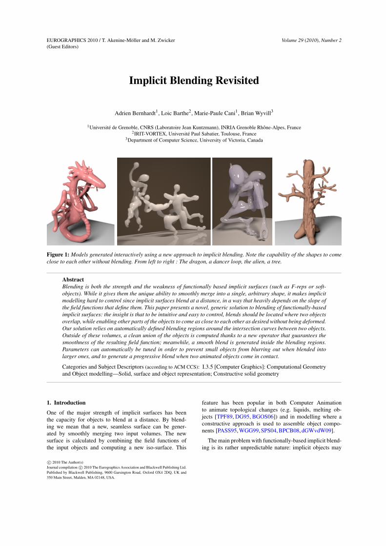
Figure 1: Models generated interactively using a new approach to implicit blending. Note the capability of the shapes to comeclose to each other without blending. From left to right : The dragon, a dancer loop, the alien, a tree.

AbstractBlending is both the strength and the weakness of functionally based implicit surfaces (such as F-reps or soft-objects). While it gives them the unique ability to smoothly merge into a single, arbitrary shape, it makes implicitmodelling hard to control since implicit surfaces blend at a distance, in a way that heavily depends on the slope ofthe field functions that define them. This paper presents a novel, generic solution to blending of functionally-basedimplicit surfaces: the insight is that to be intuitive and easy to control, blends should be located where two objectsoverlap, while enabling other parts of the objects to come as close to each other as desired without being deformed.Our solution relies on automatically defined blending regions around the intersection curves between two objects.Outside of these volumes, a clean union of the objects is computed thanks to a new operator that guarantees thesmoothness of the resulting field function; meanwhile, a smooth blend is generated inside the blending regions.Parameters can automatically be tuned in order to prevent small objects from blurring out when blended intolarger ones, and to generate a progressive blend when two animated objects come in contact.

Categories and Subject Descriptors (according to ACM CCS): I.3.5 [Computer Graphics]: Computational Geometryand Object modelling—Solid, surface and object representation; Constructive solid geometry

1. Introduction

One of the major strength of implicit surfaces has beenthe capacity for objects to blend at a distance. By blend-ing we mean that a new, seamless surface can be gener-ated by smoothly merging two input volumes. The newsurface is calculated by combining the field functions ofthe input objects and computing a new iso-surface. This

feature has been popular in both Computer Animationto animate topological changes (e.g. liquids, melting ob-jects [TPF89, DG95, BGOS06]) and in modelling where aconstructive approach is used to assemble object compo-nents [PASS95, WGG99, SPS04, BPCB08, dGWvdW09].

The main problem with functionally-based implicit blend-ing is its rather unpredictable nature: implicit objects may

c© 2010 The Author(s)Journal compilation c© 2010 The Eurographics Association and Blackwell Publishing Ltd.Published by Blackwell Publishing, 9600 Garsington Road, Oxford OX4 2DQ, UK and350 Main Street, Malden, MA 02148, USA.

Bernhardt, Barthe, Cani, Wyvill / Implicit Blending Revisited

blend at distance, or in regions where it is not required. Forinstance, in simple skeleton-based implicit modelling sys-tems (such as blobby models, meta-balls, soft objects or con-volution surfaces), the blend shape is computed by taking thesum of the field functions that define the input implicit prim-itives. Therefore, the amount and range of blending heavilydepends on the slopes of these functions, without any intu-itive user control. This results in the blurring of small, sharpfeatures when blended into large, smooth surfaces [WW00].Moreover, this is a major problem in Computer Animation,since implicit objects that come close together will start todeform and blend at a distance; for example a falling drop ofwater deforms the water surface before reaching it. Lastly,this method leads to blending in unexpected regions; for in-stance the hand of a character will blend with its body whenit comes close enough, due to the blend allowed in the shoul-der region.

Although improving control and localizing blends hasbeen attempted for years through the definition of variousways to combine field functions (see section 1.2), no simple,generally applicable solution has emerged. This may be themain reason for the relatively small spread of implicit tech-niques among the set of practical tools used by modellingand animation professionals.

We describe an automatic way of defining a blend be-tween arbitrary functionally-based implicit surfaces. Con-trary to previous methods, it does not allow objects to blendat a distance, but rather automatically localizes the blendnear the regions where their surfaces intersect, while the ex-tent of the blend is controlled independently of the supportsize of the defining field functions. This method is genericin the sense that our solution supports both local and globalsupport implicit primitives.

1.1. Technical background

An implicit surface is defined as a set of points verify-ing an equation of the type f (P) = C where f is a fieldfunction which can either be of global or local support.Other terminologies have been used for these functionssuch as potential fields in the case of skeleton-based im-plicit surfaces or implicit functions, which is not mathe-matically correct since the function is explicitly defined.We prefer field function, which expresses the fact that thatthe implicit surface is an iso-surface of the scalar fieldthey define. The field function can be defined either witha level-set, i.e. as a front propagation in a grid [Set99,OF02], or by a functionally-based representation such asf-reps [PASS95], soft objects [WMW86], convolution sur-faces [She99], RBF [SPOK95], and MLS [Lev03].

For these representations, several conventions can beused: Most global support field functions used in solid mod-elling behave as a distance to the surface of interest: theyare negative inside the object, and positive outside, C be-ing equal to zero. In contrast many implicit modelling tech-niques rely on a skeleton-based scalar field (from Blinn’s

objects to the most recent convolution surfaces): in whichcase the field function is a decreasing function of the dis-tance to a geometric primitive called the skeleton. The fieldvalues are larger inside than outside and C is non-zero. Lo-cal support implicit surfaces such as meta-balls and softobjects belong to that group, with fields that vanish at agiven distance to the skeleton. All these representations havespecific properties that lead to different composition opera-tors for union, difference, blending, etc. For a full explana-tion please see [BWd04]. This paper does not focus on dis-cretely sampled distance fields, like level sets, but rather onthe blending of functionally based implicit surfaces.

1.2. Previous work

Over the years, improving the control of implicit blends andlocalizing them (i.e. solving the unwanted blending prob-lem) has been a major area of research in implicit modellingand animation. While efficient solutions have been proposedfor level set implicit surfaces [MBWB02,BMPB08,EGB09],no fully satisfactory technique has been developped forfunctionally-based implicit surfaces. Up to now, two fami-lies of solutions arose: The first ones used a blending graphto define pairs of primitives allowed to blend, i.e. to sum theirfield functions. Since the early solutions [GW95, DG95] didnot insure that the resulting shape was continuous every-where or could lead to sudden shape changes during an-imation, more elaborate methods were developed [CH01,AC02]. In particular, Angelidis [AC02] added decay func-tions to skeletal elements to insure the smoothness of theresulting shape, making the method quite intricate to im-plement and restricting the method to the specific case ofconvolution surfaces generated by skeletons made of line-segments and triangles.

A second group of methods developed more powerfulways than simple sums to combine scalar fields. In his sem-inal paper on set-theoretic R-functions [PASS95], A. Paskointroduced, in the framework of the global support surfacesused in solid modelling, Rvashev’s R-function union opera-tor that generates at the same time, the exact (sharp) unionsurface and a C1 continuous field function everywhere else.In the remainder of this paper, we will call such an operatora clean union since it ensures that no unexpected crease ap-pears during subsequent blends [BWd04]. More recently G.Pasko [PPK05] proposed a method for defining local smoothblends between some parts of two objects, while using aclean union elsewhere. This was done through the specifica-tion of a simple user-defined implicit primitive (sphere, el-lipse, torus) of local support, indicating the blending region.The field function of the primitive was used to control theamount of blending. This method was designed for globalsupport implicit surfaces and required manual user interven-tion to tune each blend.

In parallel, Barthe [BDS∗03, BWd04] developed control-lable ways to blend field functions. The method, first in-troduced for global support implicit surfaces, offered intu-itive shape parameters and enabled the accurate location of

c© 2010 The Author(s)Journal compilation c© 2010 The Eurographics Association and Blackwell Publishing Ltd.


the blend between two given iso-values of the input implicitfunctions. However this does not allow some parts of thesurfaces to come close without blending.

Barthe later extended his operator for soft objects (of localsupport) and defined the first clean union. However, his solu-tion based on arcs of ellipses is computationally very costly,and thus not practical in an interactive modelling system.Lastly, the smooth blend operator was used in a sketch-basedmodelling system [BPCB08], where blends were artificiallylocalized by re-computing only a part of the iso-surface. Thismethod could lead to artefacts during subsequent blends dueto the lack of implicit representation for the whole surface.

1.3. Overview and contributions

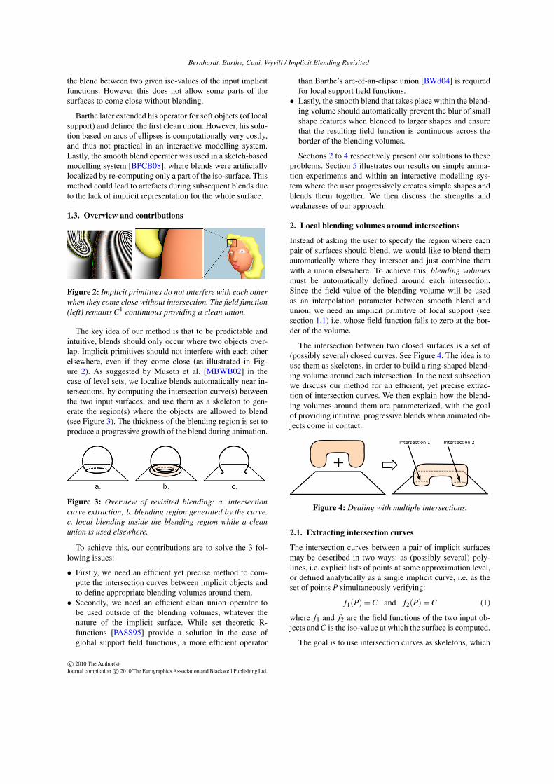
Figure 2: Implicit primitives do not interfere with each otherwhen they come close without intersection. The field function(left) remains C1 continuous providing a clean union.

The key idea of our method is that to be predictable andintuitive, blends should only occur where two objects over-lap. Implicit primitives should not interfere with each otherelsewhere, even if they come close (as illustrated in Fig-ure 2). As suggested by Museth et al. [MBWB02] in thecase of level sets, we localize blends automatically near in-tersections, by computing the intersection curve(s) betweenthe two input surfaces, and use them as a skeleton to gen-erate the region(s) where the objects are allowed to blend(see Figure 3). The thickness of the blending region is set toproduce a progressive growth of the blend during animation.

Figure 3: Overview of revisited blending: a. intersectioncurve extraction; b. blending region generated by the curve.c. local blending inside the blending region while a cleanunion is used elsewhere.

To achieve this, our contributions are to solve the 3 fol-lowing issues:

• Firstly, we need an efficient yet precise method to com-pute the intersection curves between implicit objects andto define appropriate blending volumes around them.• Secondly, we need an efficient clean union operator to

be used outside of the blending volumes, whatever thenature of the implicit surface. While set theoretic R-functions [PASS95] provide a solution in the case ofglobal support field functions, a more efficient operator

than Barthe’s arc-of-an-elipse union [BWd04] is requiredfor local support field functions.

• Lastly, the smooth blend that takes place within the blend-ing volume should automatically prevent the blur of smallshape features when blended to larger shapes and ensurethat the resulting field function is continuous across theborder of the blending volumes.

Sections 2 to 4 respectively present our solutions to theseproblems. Section 5 illustrates our results on simple anima-tion experiments and within an interactive modelling sys-tem where the user progressively creates simple shapes andblends them together. We then discuss the strengths andweaknesses of our approach.

2. Local blending volumes around intersections

Instead of asking the user to specify the region where eachpair of surfaces should blend, we would like to blend themautomatically where they intersect and just combine themwith a union elsewhere. To achieve this, blending volumesmust be automatically defined around each intersection.Since the field value of the blending volume will be usedas an interpolation parameter between smooth blend andunion, we need an implicit primitive of local support (seesection 1.1) i.e. whose field function falls to zero at the bor-der of the volume.

The intersection between two closed surfaces is a set of(possibly several) closed curves. See Figure 4. The idea is touse them as skeletons, in order to build a ring-shaped blend-ing volume around each intersection. In the next subsectionwe discuss our method for an efficient, yet precise extrac-tion of intersection curves. We then explain how the blend-ing volumes around them are parameterized, with the goalof providing intuitive, progressive blends when animated ob-jects come in contact.

Figure 4: Dealing with multiple intersections.

2.1. Extracting intersection curves

The intersection curves between a pair of implicit surfacesmay be described in two ways: as (possibly several) poly-lines, i.e. explicit lists of points at some approximation level,or defined analytically as a single implicit curve, i.e. as theset of points P simultaneously verifying:

f1(P) = C and f2(P) = C (1)

where f1 and f2 are the field functions of the two input ob-jects and C is the iso-value at which the surface is computed.

The goal is to use intersection curves as skeletons, which



generate implicit volumes, i.e. to enable quick yet precisedistance queries from arbitrary points in space to the curves.In [MBWB02], the intersection curves computation relieson the discrete grid representation of the potential field. Forfunctionally-based field functions, such a discrete represen-tation is not directly available. In the first case, a distancequery can be made efficient by embedding the poly-line intoa tree of bounding boxes, but the resolution being fixed, pre-cision may be lacking. In the second case, precision is goodsince the curve is analytically defined, but distance queriesmay not be efficient, since a numeric technique must be usedto find the closest curve point.

To get both precision and efficiency, we use a hybrid ap-proach: We first extract low resolution versions of the curves,and we locally refine each curve by splitting segments inwhich the mid-point does not meet the constraint presentedin Equation 1. The extra points are made to converge on thecurve using the algorithm described in [WvO96], i.e. by al-ternately marching in the two field gradient directions.

The extraction of the low resolution curve can be donein one of two ways. Firstly, by computing the intersectionof the meshes used to display the input implicit surfaces;this is done in an efficient way using hierarchies of bound-ing boxes. The second approach uses the efficient marching-faces algorithm, introduced in [LY03]: A marching-cubesis performed on the set of voxels embedding surface in-tersections in order to locally polygonized each surface.The marching-faces algorithm then computes the intersec-tion lines of polygones in each voxel. This second methodis more general, since it does not require any precomputedmeshing of the input surface. The selection of the voxels em-bedding the intersection curve required by this last techniquecan be greatly accelerated using an adaptive octree in the in-tersection of the combined objects bounding boxes. The oc-tree splitting is guided by the well designed inclusion func-tions of f1 and f2 [FSSV06, Duf92, Sny92], which provideintervals that are close to optimal.

The method produces a fast computation of explicit yetprecise curves. In the case of multiple intersection volumes,our method has the advantage of separating the intersectioninto disjoint curve primitives, whereas the analytical descrip-tion would not. This allows us to generate blending vol-umes of appropriate size around each individual curve, asexplained next.

2.2. Setting bounding volume parameters

At this point, the intersection is described as one or sev-eral closed curve(s). We build an implicit blending volumearound each of them by using a finite support skeleton-generated field function, such as Wyvill’s soft object func-tion [WMW86] used in our current implementation. How-ever, a parameter needs to be set: the thickness of the ring-shaped blending volumes, defined as the size of the supportof the associated local field function.

As already mentioned, we are looking for a method which

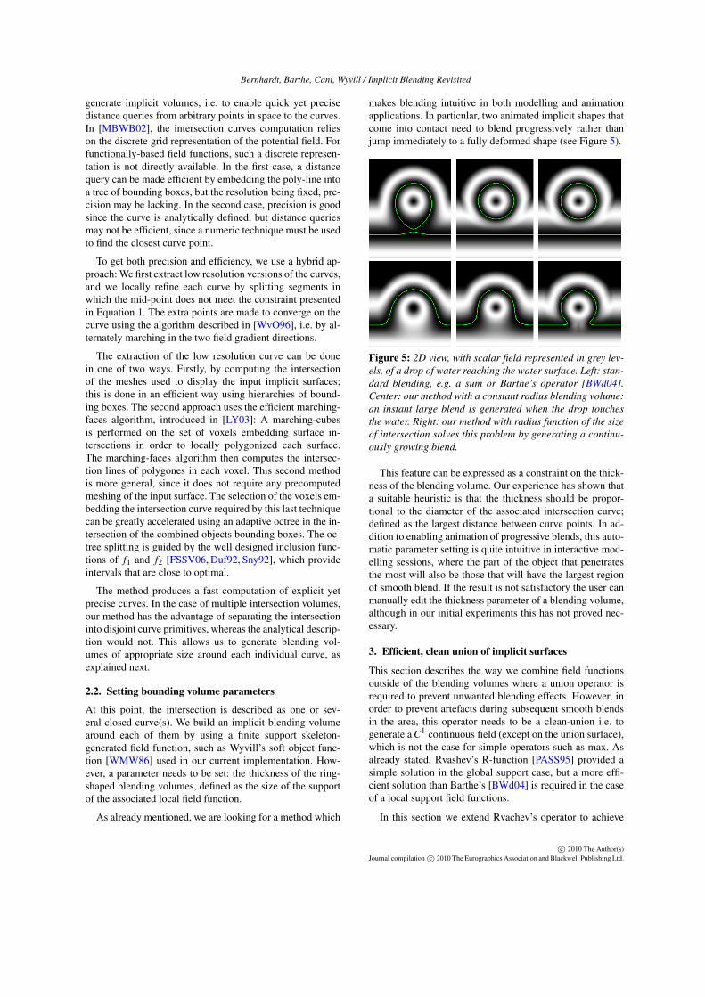
makes blending intuitive in both modelling and animationapplications. In particular, two animated implicit shapes thatcome into contact need to blend progressively rather thanjump immediately to a fully deformed shape (see Figure 5).

Figure 5: 2D view, with scalar field represented in grey lev-els, of a drop of water reaching the water surface. Left: stan-dard blending, e.g. a sum or Barthe’s operator [BWd04].Center: our method with a constant radius blending volume:an instant large blend is generated when the drop touchesthe water. Right: our method with radius function of the sizeof intersection solves this problem by generating a continu-ously growing blend.

This feature can be expressed as a constraint on the thick-ness of the blending volume. Our experience has shown thata suitable heuristic is that the thickness should be propor-tional to the diameter of the associated intersection curve;defined as the largest distance between curve points. In ad-dition to enabling animation of progressive blends, this auto-matic parameter setting is quite intuitive in interactive mod-elling sessions, where the part of the object that penetratesthe most will also be those that will have the largest regionof smooth blend. If the result is not satisfactory the user canmanually edit the thickness parameter of a blending volume,although in our initial experiments this has not proved nec-essary.

3. Efficient, clean union of implicit surfaces

This section describes the way we combine field functionsoutside of the blending volumes where a union operator isrequired to prevent unwanted blending effects. However, inorder to prevent artefacts during subsequent smooth blendsin the area, this operator needs to be a clean-union i.e. togenerate a C1 continuous field (except on the union surface),which is not the case for simple operators such as max. Asalready stated, Rvashev’s R-function [PASS95] provided asimple solution in the global support case, but a more effi-cient solution than Barthe’s [BWd04] is required in the caseof a local support field functions.

In this section we extend Rvachev’s operator to achieve



the clean-union of local support implicit surfaces, in an effi-cient manner, and more generally of any skeleton-based im-plicit surface, including global support blobs and convolu-tion surfaces. Figure 6 illustrates the different steps of ourmethod.

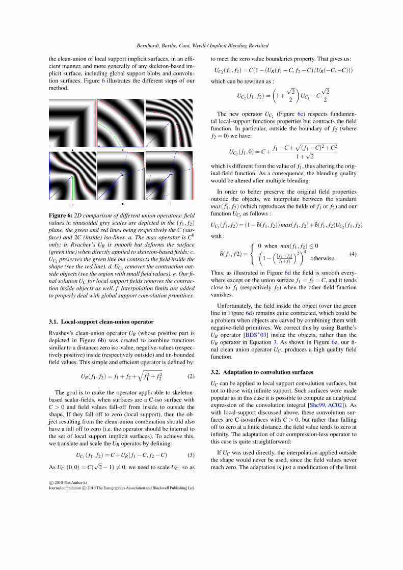
Figure 6: 2D comparison of different union operators: fieldvalues in sinusoidal grey scales are depicted in the ( f1, f2)plane, the green and red lines being respectively the C (sur-face) and 2C (inside) iso-lines. a. The max operator is C0

only; b. Rvachev’s UR is smooth but deforms the surface(green line) when directly applied to skeleton-based fields; c.UC2 preserves the green line but contracts the field inside theshape (see the red line). d. UC3 removes the contraction out-side objects (see the region with small field values). e. Our fi-nal solution UC for local support fields removes the contrac-tion inside objects as well. f. Interpolation limits are addedto properly deal with global support convolution primitives.

3.1. Local-support clean-union operator

Rvashev’s clean-union operator UR (whose positive part isdepicted in Figure 6b) was created to combine functionssimilar to a distance: zero iso-value, negative-values (respec-tively positive) inside (respectively outside) and un-boundedfield values. This simple and efficient operator is defined by:

UR( f1, f2) = f1 + f2 +√

f 21 + f 2

2 (2)

The goal is to make the operator applicable to skeleton-based scalar-fields, when surfaces are a C-iso surface withC > 0 and field values fall-off from inside to outside theshape. If they fall off to zero (local support), then the ob-ject resulting from the clean-union combination should alsohave a fall off to zero (i.e. the operator should be internal tothe set of local support implicit surfaces). To achieve this,we translate and scale the UR operator by defining:

UC1( f1, f2) = C +UR( f1−C, f2−C) (3)

As UC1(0,0) = C(√

2− 1) 6= 0, we need to scale UC1 so as

to meet the zero value boundaries property. That gives us:

UC2( f1, f2) = C(1− (UR( f1−C, f2−C)/UR(−C,−C)))

which can be rewriten as :

UC2( f1, f2) =(

1+√

22

)UC1 −C

√2

2

The new operator UC2 (Figure 6c) respects fundamen-tal local-support functions properties but contracts the fieldfunction. In particular, outside the boundary of f2 (wheref2 = 0) we have:

UC2( f1,0) = C +f1−C +

√( f1−C)2 +C2

1+√

2

which is different from the value of f1, thus altering the orig-inal field function. As a consequence, the blending qualitywould be altered after multiple blending.

In order to better preserve the original field propertiesoutside the objects, we interpolate between the standardmax( f1, f2) (which reproduces the fields of f1 or f2) and ourfunction UC2 as follows :

UC3( f1, f2) = (1−δ( f1, f2))max( f1, f2)+δ( f1, f2)UC2( f1, f2)

with :

δ( f1, f 2) =

0 when min( f1, f2)≤ 0(

1−(| f1− f2|

f1+ f2

)2)4

otherwise.(4)

Thus, as illustrated in Figure 6d the field is smooth every-where except on the union surface f1 = f2 = C, and it tendsclose to f1 (respectively f2) when the other field functionvanishes.

Unfortunately, the field inside the object (over the greenline in Figure 6d) remains quite contracted, which could bea problem when objects are carved by combining them withnegative-field primitives. We correct this by using Barthe’sUB operator [BDS∗03] inside the objects, rather than theUR operator in Equation 3. As shown in Figure 6e, our fi-nal clean union operator UC, produces a high quality fieldfunction.

3.2. Adaptation to convolution surfaces

UC can be applied to local support convolution surfaces, butnot to those with infinite support. Such surfaces were madepopular as in this case it is possible to compute an analyticalexpression of the convolution integral [She99, AC02]). Aswith local-support discussed above, these convolution sur-faces are C-isosurfaces with C > 0, but rather than fallingoff to zero at a finite distance, the field value tends to zero atinfinity. The adaptation of our compression-less operator tothis case is quite straightforward:

If UC was used directly, the interpolation applied outsidethe shape would never be used, since the field values neverreach zero. The adaptation is just a modification of the limit



after which the operator reproduces f1 and f2 fields. To doso, we modify δ (Equation 4) so that δc( f1, f2) = 0 whenf1 = α1 f2 or f2 = α2 f1 :

δc( f1, f2) =

{0 when f1 ≤ α1 f2 or f2 ≤ α2 f1(

4( f1−α1 f2)( f2−α2 f1)((1−α2) f1+(1−α1) f2)

)2otherwise.

Once this is done, we still use Barthe’s UB operator insidethe objects in order to take into account the limit parametersα1 and α2 while providing a high quality field function (seeFigure 6f).

4. Local, smooth blends

In this section we discusse our choice of operator inside theblending volume. As stressed in the introduction, the goalis to automatically calibrate a smooth blending operator inorder to prevent the blurring of small shapes when blendedinto large, smooth ones. Our operator should also insure aseamless transition with the outer region, where the clean-union is used. The two following sections address these twoproblems.

4.1. Detail-preserving smooth blend

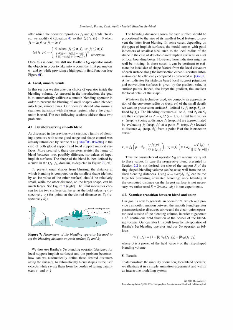
As discussed in the previous work section, a family of blend-ing operators with some good range and shape control wasalready introduced by Barthe et al. [BDS∗03,BWd04] in thecase of both global support and local support implicit sur-faces. More precisely, these operators restrict the range ofblend between two, possibly different, iso-values of inputimplicit surfaces. The shape of the blend is then defined bya curve in the ( f1, f2) domain, as depicted in Figure 7 (left).

To prevent small shapes from blurring, the distance atwhich blending is computed on the smallest shape (definedby an iso-value of the other surface) should be relativelysmall, while the other distance, on the larger shape, can bemuch larger. See Figure 7 (right). The limit iso-values cho-sen for the two surfaces can be set as the field values v1 (re-spectively v2) for points at the desired distance on S1 (re-spectively S2).

Figure 7: Parameters of the blending operator UB used toset the blending distance on each surface S1 and S2.

We thus use Barthe’s UB blending operator (designed forlocal support implicit surfaces) and the problem becomes:how can we automatically define these desired distancesalong the surfaces, to automatically blend shapes as the userexpects while saving them from the burden of tuning param-eters v1 and v2 ?

The blending distance chosen for each surface should beproportional to the size of its smallest local feature, to pre-vent the latter from blurring. In some cases, depending onthe types of implicit surfaces, the model comes with goodindicators of smallest size, such as the local radius of theshape in the case of skeleton-based implicit surfaces, or a setof local bounding boxes. However, these indicators might aswell be missing. In these cases, it can be pertinent to esti-mate the local size of shape feature from the local curvatureof each surface along the intersection curve. Curvature infor-mation can be efficiently computed as presented in [Gol05].A last indicator for skeleton based local support primitivesand convolution surfaces is given by the gradient value atsurface points. Indeed, the larger the gradient, the smallestthe local detail of the shape.

Whatever the technique used, we compute an approxima-tion of the curvature radius r1 (resp. r2) of the small detailswe want to preserve on surface S1 defined by f1 (resp. S2 de-fined by f2). The blending distances d1 on S1 and d2 on S2are then computed as di = ri/2 (i = 1,2). Limit field valuesv1 (resp. v2) being at distance d1 (resp. d2) are approximatedby evaluating f2 (resp. f1) at a point P1 (resp. P2) locatedat distance d1 (resp. d2) from a point P of the intersectioncurve:

v1 = f2

(p+d1.

5 f2(p)‖5 f2(p)‖

), v2 = f1

(p+d2.

5 f1(p)‖5 f1(p)‖

)Thus the parameters of operator UB are automatically set

to these values. In case the progressive blend presented inSection 2.2 is not desired, the size of the support R of thering-shaped blending volume can be set as well from the de-sired blending distances. Using R = max(d1,d2) can be toolarge for preventing unwanted blending; since blending atthe computed distance on the largest surface is not neces-sary, we rather used R = 2min(d1,d2) in our experiments.

4.2. Seamless transition between blend and union

Our goal is now to generate an operator U , which will pro-vide a smooth transition between the smooth blend operatorparameterized as discussed above and the clean-union opera-tor used outside of the blending volume, in order to generatea C1 continuous field function at the border of the blend-ing volume. Our operator U is built from the interpolation ofBarthe’s UB blending operator and our UC operator as fol-lows:

U( f1, f2) = (1−β)UC( f1, f2)+βUB( f1, f2)

where β is a power of the field value v of the ring-shapedblending volume.

5. Results

To demonstrate the usability of our new, local blend operator,we illustrate it in a simple animation experiment and withinan interactive modelling system.



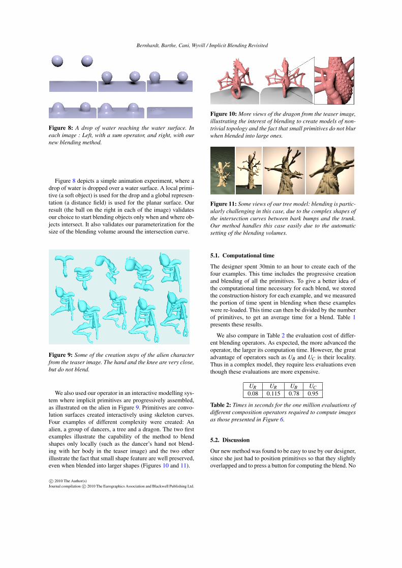
Figure 8: A drop of water reaching the water surface. Ineach image : Left, with a sum operator, and right, with ournew blending method.

Figure 8 depicts a simple animation experiment, where adrop of water is dropped over a water surface. A local primi-tive (a soft object) is used for the drop and a global represen-tation (a distance field) is used for the planar surface. Ourresult (the ball on the right in each of the image) validatesour choice to start blending objects only when and where ob-jects intersect. It also validates our parameterization for thesize of the blending volume around the intersection curve.

Figure 9: Some of the creation steps of the alien characterfrom the teaser image. The hand and the knee are very close,but do not blend.

We also used our operator in an interactive modelling sys-tem where implicit primitives are progressively assembled,as illustrated on the alien in Figure 9. Primitives are convo-lution surfaces created interactively using skeleton curves.Four examples of different complexity were created: Analien, a group of dancers, a tree and a dragon. The two firstexamples illustrate the capability of the method to blendshapes only locally (such as the dancer’s hand not blend-ing with her body in the teaser image) and the two otherillustrate the fact that small shape feature are well preserved,even when blended into larger shapes (Figures 10 and 11).

Figure 10: More views of the dragon from the teaser image,illustrating the interest of blending to create models of non-trivial topology and the fact that small primitives do not blurwhen blended into large ones.

Figure 11: Some views of our tree model: blending is partic-ularly challenging in this case, due to the complex shapes ofthe intersection curves between bark bumps and the trunk.Our method handles this case easily due to the automaticsetting of the blending volumes.

5.1. Computational time

The designer spent 30min to an hour to create each of thefour examples. This time includes the progressive creationand blending of all the primitives. To give a better idea ofthe computational time necessary for each blend, we storedthe construction-history for each example, and we measuredthe portion of time spent in blending when these exampleswere re-loaded. This time can then be divided by the numberof primitives, to get an average time for a blend. Table 1presents these results.

We also compare in Table 2 the evaluation cost of differ-ent blending operators. As expected, the more advanced theoperator, the larger its computation time. However, the greatadvantage of operators such as UB and UC is their locality.Thus in a complex model, they require less evaluations eventhough these evaluations are more expensive.

UR UR UB UC0.08 0.115 0.78 0.95

Table 2: Times in seconds for the one million evaluations ofdifferent composition operators required to compute imagesas those presented in Figure 6.

5.2. Discussion

Our new method was found to be easy to use by our designer,since she just had to position primitives so that they slightlyoverlapped and to press a button for computing the blend. No



Dragon Dancer Loop Alien TreeNb of primitives 68 23 24 54

Reconstruction time from a script 277 34.3 41.9 475Average time per primitive 2.65 1.24 1.31 6.3

Average time per blend 1.43 0.25 0.43 2.48

Table 1: Computation times in seconds required by the creation of models presented in the teaser. The second row givesthe number of primitives built by the user and then blended by the system. The third row gives, for each model, the totalcomputational time spent when they are directly created from a script. The fourth and the fifth rows give the average of the timesspent in respectively creating individual primitives and evaluating our blending operator per transition.

extra primitives had to be created nor was it necessary to tuneany parameters. The three long-standing problems identifiedfor standard implicit blending, namely unpredictable blend-ing at distance, lack of locality, and blurring of small detailswere solved by the system. The smoothness of the field func-tion after each local blend, and the fact that our union oper-ator does not create any unwanted contraction of the field,enabled the designer to create complex models without anyproblem or unexpected behaviour during successive blends.

A side benefit of our approach is the new clean union op-erator that can be used on its own for combining objectswhen a sharp union is desired.

We also identified some weaknesses of our methods, onwhich we are currently working:

Firstly, our current implementation defines blending vol-umes using a simple local support model (a soft object).Since the latter is based on the closest distance to the in- ter-section curve, this model generates a field that may not be C1

in the concavities of the curve. No artefact was ob- served inpractice: the radius of the blending volume is often smallerthan the curve radius and moreover, most curve concavitiesare inside objects. We can however see the problem on thebottom right of Figure 5, where the field looks strange in-side the implicit shape, where the plane and the drop blend.Defining blending volumes from local-support convolutionprimitives would solve the problem since it would insure C1

continuity of the scalar field everywhere and in all cases.

Secondly, the way we identify the size of small featuresfor setting up the blending parameters may not be as generalas we would like: in some cases, the two shapes we wouldlike to blend may already have some tiny details (such asbumps on the surface), while the blend should take placeat a much larger scale. In general, analysing the differentscales of details in the frequency domain and enabling theuser to choose the blending range among those scales (or do-ing it automatically from the size of the intersection curve)could be a better solution. If noisy reconstructed modelsfrom scanned real objects were used, such analyses wouldbe necessary, however, this did not make our system less us-able in practice, since objects are built from scratch and thedesigner naturally defined each object from coarse to fine.

Lastly, although our method is usable in interactive mod-elling sessions, the user sometimes has to wait for a few sec-

onds before the surface updates. This is mainly due to thelack of optimization of our polygonizer, and making blend-ing and subsequent local re-meshing real-time would be agood practical improvement. Future work includes more ac-curate incremental polygonization, a GPU implementationof our method using, for instance the Intel Larabee architec-ture.

6. Conclusion and future work

This work has taken a new look at functionally-based im-plicit surface modelling. Instead of letting surfaces blendrather imprecisely at a distance as in current systems, wepropose limiting the blend volume to where surfaces overlap,while enabling models to come close to each other every-where else without deforming. This new approach combinesthe strength of implicit surfaces, i.e. their ability to blendseamlessly, with the ease of use of more standard modelsthat do not blend. Our solution is generic and makes implicitsurfaces much easier to use for both implicit modelling andanimation.

As most previous methods [BDS∗03, BWd04, PPK05],our approach defines a binary blending operator, acting ona pair of input surfaces, whereas ’sum’ could be n-ary.

Consequently, if, for example, a group of implicit prim-itives with three overlapping blending volumes, are to becombined, the final shape will depend on the order in whichthe blends are performed. This is not a problem in an in-teractive modelling system where the user defines and addsshape components one by one, but this could be a weaknessfor procedural modelling, where complex, symmetric shapeswith multiple branching parts are to be processed. Definingmultiple-local blend operators would thus be a good topicfor future work.

Also, if the user designs a very complex object composedof both large primitives and a lot of very small details, allcomposed using our blending operator, the correct compu-tation of the intersection curves will become an issue and ascalable technique will have to be developed.

Lastly, our method offers a good solution to the unwantedblending problem when different primitives are combined,but does not address the self-blending of a single, compleximplicit surface. For example modelling a folded snake usinga convolution surface defined by a spiral curve as skeleton



is still impossible (except using intricate convolution spe-cific methods [AJC02]), since the snake would self blend.In this case, artificially cutting the object into pieces and re-blending them would solve the problem, but this could berather time consuming. A more general solution, that onlyenables blend where a complex shape self-overlaps, wouldbe a good extension to our method.

In conclusion, we hope that our new vision offunctionally-based implicit blending will be found inspiring,generate more research in the area and contribute to makeimplicit modelling more popular.

References[AC02] ANGELIDIS A., CANI M.: Adaptive implicit modeling

using subdivision curves and surfaces as skeletons. In Proceed-ings of the seventh ACM symposium on Solid modeling and ap-plications (2002), ACM New York, NY, USA, pp. 45–52.

[AJC02] ANGELIDIS A., JEPP P., CANI M.-P.: Implicit Model-ing with Skeleton Curves: Controlled Blending in Contact Situ-ations. In International Conference on Shape Modeling (2002),pp. 137–144.

[BDS∗03] BARTHE L., DODGSON N. A., SABIN M. A.,WYVILL B., GAILDRAT V.: Two-dimensional potential fieldsfor advanced implicit modeling operators. Computer GraphicsForum 22, 1 (2003), 23–33.

[BGOS06] BARGTEIL A. W., GOKTEKIN T., O’BRIEN J. F.,STRAIN J. A.: A semi-lagrangian contouring method for fluidsimulation. ACM Trans. Graph. 25, 1 (2006), 19–38.

[BMPB08] BRODERSEN A., MUSETH K., PORUMBESCU S.,BUDGE B.: Geometric texturing using level sets. IEEE Trans-actions on Visualization and Computer Graphics 14, 2 (2008),277–288.

[BPCB08] BERNHARDT A., PIHUIT A., CANI M.-P., BARTHEL.: Matisse: Painting 2D regions for modeling free-form shapes.In EUROGRAPHICS Workshop on Sketch-Based Interfaces andModeling, SBIM 2008, June, 2008 (Annecy, France, June 2008),Alvarado C., Cani M.-P., (Eds.), pp. 57–64.

[BWd04] BARTHE L., WYVILL B., DE GROOT E.: Controllablebinary csg operators for “soft objects”. International Journal ofShape Modeling 10, 2 (2004), 135–154.

[CH01] CANI M.-P., HORNUS S.: Subdivision-curve primitives:A new solution for interactive implicit modeling. Shape Model-ing and Applications, International Conference on (2001), 0082.

[DG95] DESBRUN M., GASCUEL M.: Animating soft substanceswith implicit surfaces. In SIGGRAPH’95 Conference Proceed-ings (Los Angeles, CA, Aug. 1995), Annual Conference Series,ACM SIGGRAPH, Addison Wesley, pp. 287–290.

[dGWvdW09] DE GROOT E., WYVILL B., VAN DE WETER-ING H.: Locally restricted blending of blobtrees. Computers& Graphics (2009).

[Duf92] DUFF T.: Interval arithmetic and recursive subdivisionfor implicit functions and constructive solid geometry. In Com-puter Graphics (Proceedings of SIGGRAPH 92) (1992), pp. 131–138.

[EGB09] EYIYUREKLI M., GRIMM C., BREEN D.: EditingLevel-Set Models with Sketched Curves. In Proceedings of Euro-graphics/ACM Symposium on Sketch-Based Interfaces and Mod-eling (2009), pp. 45–52.

[FSSV06] FLÓREZ J., SBERT M., SAINZ M. A., VEHÍ J.: Im-proving the Interval Ray Tracing of Implicit Surfaces. In Com-puter Graphics International 2006 (2006), pp. 655–664.

[Gol05] GOLDMAN R.: Curvature formulas for implicit curvesand surfaces. Computer Aided Geometric Design 22, 7 (2005),632–658.

[GW95] GUY A., WYVILL B.: Controlled blending for implicitsurfaces using a graph. In Implicit Surfaces’95—the First Euro-graphics Workshop on Implicit Surfaces (Grenoble, France, Apr.1995), pp. 107–112.

[Lev03] LEVIN D.: Mesh-Independent Surface Interpolation.In Geometric Modeling for ScientiïnAc Visualization (2003),pp. 181–187.

[LY03] LJUNG P., YNNERMAN A.: Extraction of intersectioncurves from iso-surfaces on co-located 3d grids. In SIGRAD2003Proceedings, ISSN 1650-3686 (2003), Linkoping ElectronicConference Proceedings, pp. 1650–3740.

[MBWB02] MUSETH K., BREEN D. E., WHITAKER R. T.,BARR A. H.: Level Set Surfaces Editing Operators. In Pro-ceedings of SIGGRAPH’02 (2002), ACM, pp. 330–338.

[OF02] OSHER S. J., FEDKIW R. P.: Level Set Methods and Dy-namic Implicit Surfaces, 1 ed. Springer, October 2002.

[PASS95] PASKO A., ADZHIEV V., SOURIN A., SAVCHENKOV.: Function representation in geometric modeling: concepts,implementation and applications. The Visual Computer 11, 8(1995), 429–446.

[PPK05] PASKO G. I., PASKO A. A., KUNII T. L.: Boundedblending for Function-Based shape modeling. IEEE Comput.Graph. Appl. 25, 2 (2005), 36–45.

[Set99] SETHIAN J. A.: Level Set Methods and Fast MarchingMethods: Evolving Interfaces in Computational Geometry, FluidMechanics, Computer Vision, and Materials Science, 2 ed. Cam-bridge University Press, June 1999.

[She99] SHERSTYUK A.: Kernel functions in convolution sur-faces: a comparative analysis. The Visual Computer 15, 4 (1999),171–182.

[Sny92] SNYDER J. M.: Interval analysis for computer graphics.In Computer Graphics (Proceedings of SIGGRAPH 92) (1992),pp. 121–130.

[SPOK95] SAVCHENKO V. V., PASKO A., OKUNEV O. G., KU-NII T. L.: Function representation of solids reconstructed fromscattered surface points and contours. Computer Graphics Forum14, 4 (1995), 181–188.

[SPS04] SCHMITT B., PASKO A. A., SCHLICK C.: Constructivesculpting of heterogeneous volumetric objects using trivariate b-splines. The Visual Computer 20, 2-3 (2004), 130–148.

[TPF89] TERZOPOULOS D., PLATT J., FLEISHER K.: Heatingand melting deformable models (from goop to glop). In GraphicsInterface’89 (London, Ontario, June 1989), pp. 219–226.

[WGG99] WYVILL B., GUY A., GALIN E.: Extending the csgtree - warping, blending and boolean operations in an implicitsurface modeling system. Comput. Graph. Forum 18, 2 (1999),149–158.

[WMW86] WYVILL G., MCPHEETERS C., WYVILL B.: DataStructure for Soft Objects. The Visual Computer 2, 4 (February1986), 227–234.

[WvO96] WYVILL B., VAN OVERVELD K.: Polygonization ofImplicit Surfaces with Constructive Solid Geometry. Journal ofShape Modelling 2, 4 (1996), 257–274.

[WW00] WYVILL B., WYVILL G.: Better blending of implicitobjects at different scales. In ACM Siggraph 2000 Sketch Pro-ceedings (2000), ACM.


Implicit Blending Revisited

Documents

Transcript of Implicit Blending Revisited