AN ......u ....

IMPLEMENTING VEHICLE ROUTING ALGORITHMSHam.:by

!hu:MBRUCE L. GOLDENa Hm THOMAS"L. -MAGNANTI,

p andHIEN:-0. NGUYEN,

.......... ............... '::,:-..':................................ .... ................

............................ ............. ....... ....... . ....... ......:. .t.

Techncl Repot No 115,

'OPERATON ESEARHCNE

Jlfl

~ :1: ~. . ASSACUS 7 S INSTITUTE:

TECHNOLOGY,; D16T

4etembeor 1975.

DISCLAIMER NOTICE

THIS DOCUMENT IS BEST QUALITYPRACTICABLE. THE-COPY FURNISHEDTO DTIC CONTAINED A SIGNIFICANTNUMBER OF PAGES WHICH DO NOTREPRODUCE LEGIBLY.

Vi"

A~CESSIO0tQ

... .~ .........~C~CEO- £

AIL2L~

UnclassifiedSECURITY CLASSIFICATION OF THIS PAGE W'(en Data ntered)

REPORT DOCUMENTATION PAGE BEFREAD INSTRUCTIONSI~Lr~l UUMLII~III1 ~BEFORE COMPLETING FORM1. REPORT NUMBER 2. GOVT ACCESSION NO. 3. RECIPIENT'S CATALOG NUMBER

Technical Report No. 115A. "TITLE (and St bettio) S "rYPE_ ('aF RI BZJ T RL COVE.RED

( t ) 0bTechnical /eP6.i-t"IEPICLE ROUTING ALGORITHMS,.

T I lPLEME3N GlNG

PERFORMING ORG. REPORT NUMBER

"I , AUTHORff IRS S. CONTRACT OR GRANT NUMBER(&)Bruce L. ;,olde , ,_ /-

Thomas L. IMagnani/Hien Q./Nguven__________ ______________PERFORMING ORGANIZATION NAME AND ADDRESS t ASK

M.I.T. Operations Research Center AREA & WORK UNIT NUMBERS

77 Massachusetts Avenue, Room 24-215 NR-347-/27Cambridge, M,% 02139

11. CONTROLLING 0 "FICE NAME AND ADDRESS 12. REPORT DATEO.R. Branch. ONR Navy Dept. Sepe -- 75JArlington, VA 22217 .I. 46

14 MONITORING AGENCY NAME & AODRESS(II different Irom C)ttotlng Office) iS. SECURITY CLASS. (of this report)

Unclassif ied

15n. DECL ASSI FICATION/DOWN GRADINGSCHEDULE

16. DISTRIBUTION STATEMENT (of Chia Report)ReIe~,b fcou iiiLurt-lcf on d~omnto,,/- :."'rsi r

p.r,, .... Publu rolea,IY~trlbu lJni-LJ4d

17 DISTRIBUTION STATEMENT (of the abstract entered In l7mock 20, If different from Report)

18. SUPPLEMENTARY NOTES

I9. KEY WORDS (Continue on reverse aide if nuceseay mid Identify by block number)

SHeuristic ProgrammingVehicle RoutingMulti-Depot Routing Algorithm

20.t BSTRACT (Continue on reverse side If necessary and identify by block number)

euristic programming algorithms frequently address large problems and requiremanipulation and operation on massive data sets. The algorithms can be im-proved by using efficient data structures. With this in mind, we considerheuristic algorithms for vehicle routing, comparing techniques of Clarke andWright, Gillett and Miller, and Tyagi, and presenting modifications and ex-tensions which permit problems involving hundreds of demand points to be t "

solved in a matter of seconds. ln addition, a multi-depot routing algorithm t C

DD 1 JAN73 1473 EDITION OF I NOV 65IS OBSOLETE Unclassified O 7o26SECURITY CLASSIFICATION OF MIS PAGE (When Date Entered)

i UnclassifiodSECUAIrTYLASSTFICATIOM OF THIS PAOE(W7,n Data Ent.d)-

is developed. The results are ilJustrated with a routing study for anurban newspaper witlh an evening circulation exceeding 100,000.

Unclassified

SECkIRITY :LASSIFICATION OF THIS PAGE(When Dota Entered)

IMPLEMENTING VEHICLE ROUTING ALGORITHMS

by

BRUCE L. GOLDEN*THOMAS L. MAGNANTI**

andIIEN Q. NGUYEN

Technical Report No. 115

Operations Research Center

Massachusetts Institute of Technology

Cambridge, Massachusetts 02139 d "

'! "

September 1975

\ p4 1 orcvo,.d fo public relc~O

* Supported in part by the American Newspapers Publishers' Associationand the Department of Transportation under Contract DOT-TSC-1058.

** Supported in part by the Office of Naval Research under Contract

N0014-75-C-0056 and in part by the Army Research Office underCont rac T5AMf4-73-C-O032.

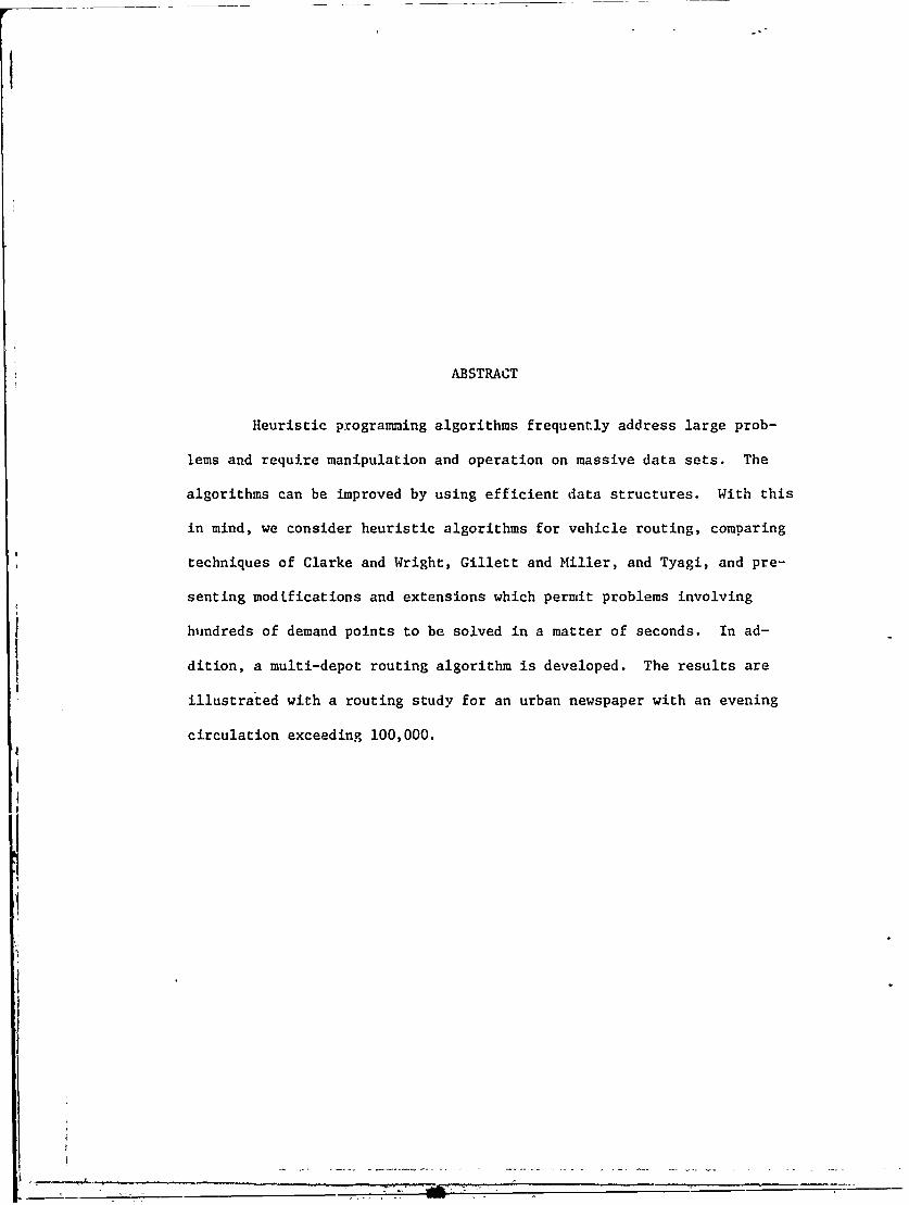
ABSTRACT

Heuristic programming algorithms frequently address large prob-

lems and require manipulation and operation on massive data sets. The

algorithms can be improved by using efficient data structures. With this

in mind, we consider heuristic algorithms for vehicle routing, comparing

techniques of Clarke and Wright, Gillett and Miller, and Tyagi, and pre-

senting modifications and extensions which permit problems involving

hundreds of demand points to be solved in a matter of seconds. In ad-

dition, a multi-depot routing algorithm is developed. The results are

illustrated with a routing study for an urban newspaper with an evening

circulation exceeding 100,000.

-1-

I. INTRODUCTION

An essential element of any logistics system is the allocation and

routing of vehicles for the purpose of collecting and delivering goods and

services on a regular basis. Common examples include newspaper delivery [29],

schoolbus routing [8], municipal waste collection [71, fuel oil delivery [25],

and truck dispatching in any of a number of industries. The system may in-

volve a single depot or multiple depots; the objectives may be aimed at

cost minimization (distribution costs, and vehicle or depot acquisition costs)

or service improvement (increasing distribution capacities, reducing distri-

bution time, and related network design issues). Constraints may be imposed

upon

i) the depots (numbers, possible locations, and production

capabilities),

(ii) the vehicle fleet (types and numbers of vehicles, andvehicle capacities),

(iii) the delivery points (demand requirements, service con-straints on delivery time, and order splitting),

(iv) the routing structure (maximum route time or route

distance, link capacities, and preferences for radialroutes, peripheral routes, or routes with points closer

together),

(v) operator scheduling and assignments (union regulations),

and (vi) system dynamics (inventory holdings, and distribution

or acquisition lag times).

Applications emphasizing various of these characteristics lead to a

continuum of overlapping models including location models such as median

and minimax location, scheduling models such as crew scheduling, distribution

models such as minimum cost flow or shortest paths, or location-distribution

-2-

models such as warehouse location. In this paper, we consider models of the

routing type with fixed depots, constrained for the most part by fleet,

delivery point, and route structure restrictions. Our purposes are three-fold.

By synthesizing and extending the results presented in Golden [291 and

Nguyen [54], we first formulate integer programming models of these problems,

building upon the traveling salesman problem as the "core" model. We then

review the most promising heuristic solution procedures for these problems

sugges-ed in the literature. Finally, we suggest particularly fast implemen-

tations of the Clarke-Wright heuristic procedure. Our method uses efficient

data handling capabilities such as heap structures to enhance both computations

and storage. Our results indicate that algorithmic modifications of this

nature rian greatly extend the size of problems amenable to analysis.

We have applied the algorithm to a distribution system for an urban

newspaper with an evening circulation exceeding 100,000. This problem

contains nearly 600 drop points for newspaper bundles and was solved with 20

seconds of execution time on an IBM 370/168. Fast computations of this

nature permit the algorithm to be used as an operational tool and to be used

interactively to study modeling assumptions such as demand patterns. It

could be used, for example, as in our newspaper study, to investigate perfor-

mance measures associated with operating policies like the pre-routing of

important drop points on special routes. In addition, past implementation

suggests that the heuristic might be used as a subroutine for more general

problems in order to incorporate other of the distribution characteristics

delineated above, or to perform on-line dynamic routing.

We believe that our computational experience is indicative of implementa-

tions for heuristic algorithms in general. Because these algorithms frequently

- ---

-3-

replace computationally expensive or intractable formal optimization

procedures by simple, but usually extensive, addition and comparison operations,

data organization can be important. Improving data access for each basic

operation can lead to order of magnitude improvements in overall running time.

II. FORMULATIONS

The Traveling Salesman Problem

Most vehicle routing models are variants and extensions of the ubiquitous

Traveling Salesman Problem; for a very thorough overview of this problem see

Bellmore and Nemhauser [6]. Suppose we are given the matrix of pairwise

distances or costs dij between node i and node j for the n nodes 1, 2, ..., n.

We assume d = for i = 1, 2, ..., n. The problem is to form a tour of the

n nodes beginning and ending at the origin, node 1, which gives the minimum

total distance or cost. For notation, let

n = the number of nodes in the network

V = the set of nodes

1 if arc (i, j) is in the tourij 1 0 otherwise

dij = the distance on arc (i, j).

An assignment-based lormulation of the problem selects the matrix X = (x)ij of

decision variables solving:

n nMinimize E E d x (1.1)

i=l j=l ij ij

-4-

nsubject to E x = 1 (j i, ... , n) (1.2)

i=l

nE 1 (i = 1, ... , n) (1.3)

J=l

X = (xij) E S (1.4)

x .. 0 or 1 (i = 1, ... , n; (1.5)

j 1, ... , n).

The set S is selected to prohibit subtour solutions satisfying the assign-

ment constraints (1.2), (1.3), and (1.5). Several alternates have been pro-

posed for S including

(1) S = {(xij): E E xij > 1 for every nonempty

iEQ jVQ proper subset Q of V ;

(2) S = {(xij): E E xi < IQI - 1 for every nonempty

isQ jCQ subset Q of{2, 3, .. ,n}j

-< n-l for2<~~

(3) S = (xij): y y + nx -- -- --for some real numbers y i.

Note that S contains nearly 2n subtour breaking constraints in (1) and (2),

2but only n - 3n + 2 constraints in the ingenious formulation (3) proposed by

Miller, Tucker, and Zemlin [51]. Algorithmically, the constraints in (2)

have proved very useful, however, for Lagrangian approaches to the Traveling

Salesman Problem, as initiated by Held and Karp [32], [33]. For other approaches,

both heuristic and optimal, see Lin [46], Lin and Kernighan [47], Christofides

and Eilon [16], Little [48], and Shapiro [64].

-5-

The Traveling Salesman Problem can be interpreted as a vehicle routing

model with one depot and with one vehicle whose capacity exceeds total demand.

This model can be extended by considering more vehicles, more depots, different

vehicle capacities, and additional route restrictions.

The Multiple Traveling Salesmen Problem

The Multiple Traveling Salesmen Problem (MTSP) is a generalization of

the Traveling Salesman Problem (TSP) and comes closer to accomodating more

real-world problems; here there is a need to account for more than one salesman

(vehicle). Multiple Traveling Salesmen Problems arise in many sorts of

scheduling and sequencing applications. For example, the framework could be

used to develop the basic route structure for a pickup or delivery service

(perhaps a schoolbus or rural bus service); it has proved to be an appropriate

model for the problem of bank messen6 r scheduling, where a crew of messengers

picks up deposits at branch banks and returns them to the central office for

processing [65].

Given M salesmen and ii nodes in a network the MTSP is to find M subtours

(each of which includes the origin) such that every node (except origin) is

visited exactly once by exactly one sI esman- so that thc total distance Lravel-

ed by all. M salesmen is minimum. A MTSP formulation is displayed below.

Minimize Z Z d x (2.1)i=l j=l ij x

subject to Zn x = b = . if j-i (1.2)

i=l ij j if j=2, 3, .. , n

Zn x.. = a M if j=l (2.3)j=l 1 if i=2, 3, n

-6-

X (x ) S (2.4)ii

x 0 or 1 (i = 1, ..., n; (2.5)j - 1, .. n)

for any choice of the set S that breaks subtours which do not include the

origin. In particular, any of the three choices given previously for S can be

used.

Svestka and Huckfeldt [651 present a Miller-Ticker-Zemlin-like formulation

for S and apply a subtour elimination type branch and bound procedure using

Bellmore and Malone branching to obtain the optimal solution; mean run time for

55 city problems is one minute. Three different papers published in 1973

and 1974 independently derived equivalent TSP formulations of the MTSP [5],

[58], [651 and consequently showed that the M - salesmen problem is no more

difficult than its one-salesman counterpart. The equivalence is obtained by

creating m copies of the origia, each connected to the other nodes exactly

as was the original origin (with the same distances). The m copies are not

connected, or are connected by arcs each with distances exceeding

En En Id I"1. In this way, an optimal single salesman tour in the expanded

i=l j=l i

network will never use an arc connecting two copies of the origin. Then, by

coalescing the copies back into a single node, the single salesman tour decom-

poses into M subtours as required in the MTSP.

77 ..

-7-

Vehicle Dispatching

The vehicle dispatching problem was first considered by Dantzig and

Ramser [20] who developed a heuristic approach using linear programming ideas

and aggregation of nodes. The problem is to obtain a set of delivery routes

from a central depot to the various demand points, each of which has known

requirements, tc minimize the total distance covered by the entire fleet.

Vehicles have capacities and maximum route time constraints. All vehicles

start and finish at the central depot. We will refer to the following formulation

for this problem as the generic vehicle routing problem (VRP):

n n NVMinimize E E d.. x.. (3.1)

i=l j=l k=l 13 13

n NV ksubject to E x. (j 2, ... , n) (3.2)

i=l k=l

n NV k

j E x.. 1 (i = 2, ... , n) (3.3)j=l k=l 13

n k n kSX. - Z x. 0 (k = 1, ... , NV;(3.4)i=l ip j=l xPj p = i,., n)

n nZ ( E X . < Pk (k = 1, ... , NV)(3.5)

i=l j=l 1 3

n k n k n n k k

l i E x. + Z E ti. x. < Tk (k = 1, ... , NV)(3.6)i=l j=l 13 i=l j=l13 ij -- k

~n kn x < 1 (k 1,..., NV)(3.7)

j=2

-8-

n kx < 1 (k = 1, ..., NV) (3.8)

i=2

X C S (3.9)

kx.. k 0 or 1 for all i, j, k. (3.10)

iJ

where n = number of nodesNV = number of vehiclesPk = capacity of vehicle kTk = maximum time allowed for route of vehicle kQi = demand at node i CQ = 0)k

t. = time required for vehicle k to deliver or collect at node 3 (tl=0)kti k travel time for vehicle k from node i to node j (tli 0)

d.. distance from node i to node j3

k (1 if arc (i, j) is traversed by vehicle kij 0O otherwise

NV k

X matrix with components xi Z x ij , specifying connectionsk-l

regardless of vehicle type.

Equation (3.1) states that total distance is to be minimized. Alternatively,

kwe could minimize costs by replacing dij by the cost coefficient cij which

depends upon the vehicle type. Equations (3.2) and (3.3) ensure that each

demand node is served by one vehicle and only one vehicle. Route continuity

is represented by equations (3.4), ia., if a vehicle enters a demand node,

it must exit from that node. Equations (3.5) are the vehicle capacity con-

straints; similarly, equations (3.6) are the total elapsed route time con-

straints. For instance, a newspaper delivery truck may be restricted -om

spending more than one hour on a tour in order that the maximum time interval

from press to street be made as short as possible. Equations (3.7) and (3.8)

make certain that vehicle availability is not exceeded. Finally, the subtour-

n~.7

-9-

breaking constraints (3.9) can be any of the equations specified previously.

Since (3.2) and (3.4) imply (3.3), and (3.4) and (3.7) imply (3.8), from now

on we consider the generic model to include (3.1) - (3.10) exLluding (3.3)

and (3.8), which are redundant. We assume that max Qi < min Pk"l< i<n I < k <NV

That is, the demand at each node does not exceed the capacity of any truck.

Observe that when vehicle capacity constraints (3.5) and route time constraints

(3.6) are nonbinding, and can be ignored, this model reduces to a multiple

traveling salesmen problem by eliminating constraints (3.4) and substituting

NV kx.. = Z x.. in the objective function and remaining constraints.

k=l

In our generic model we have assumed that when a demand node is serviced,

its requirements are satisfied. In other words, one visit is sufficicnt. A

mixed integer programming heterogeneous fleet problem formulation was given

in 1967 by Garvin [25] in which this assumption is relaxed. The number of

,;ariables in his formulation is much greater than in the previous model where

the structure is related more closely to the formulation of the fundamental

Traveling Salesman Problem. Balinski and Quandt [4] provide another formulation

in terms of a set cove ing problem.n k

Observe that since E x. is 1 or 0 depending upon whether or not thej=2 X,

th n kk vehicle is used, a fixed acquisition cost f kL x can be added to thej=l l abeaddoth

model when it is formulated with an objective function to investigate tradeoffs

between routing and acquisition costs.

We can, without difficulty, generalize the generic model to the multi-

commodity case where several different types of products must be routed

7- -if

-10-

simultaneously over a network in order to satisfy demands at delivery points

for the various products [29].

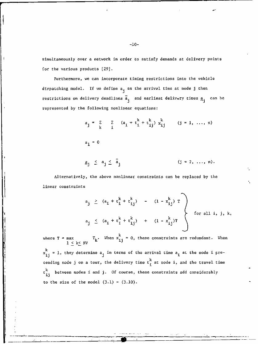
Furthermore, we can incorporate timing restrictions into the vehicle

dispatching model. If we define a. as the arrival time at node j then

restrictions on delivery deadlines a. and earliest delivury times a. can be21 -3

represented by the following nonlinear equations:

k ~kkaj Z Z (ai + t k + t kj) xik (j =,..,n)

k i ij ij

a1 0

a. < a. <a (= 2,... n)-32 - 21 - J "'" "

Alternatively, the above nonlinear constraints can be replaced by the

linear constraints

a > (ai + tik + tk) - (1- xij) T

for all i, j, k,

aj < (ai + tk + ti) + (1- Xk)Tti 121i

kwhere T = max Tk . When xjij = 0, these constraints are redundant. When

1 < k< NV

kx i = 1, they determine a. in terms of the arrival time a. at the node i pre-

kceeding node j on a tour, tihe delivery time t. at node i, and the travel timeik

tij between nodes i and j. Of course, these constraints add considerably

to the size of the model (3.1) - (3.10).

Multi-Depot Vehicle Routing

The integer programming formulation of the vehicle routing problem is

altered in minor ways to incorpoiate multiple depots. Letting nodes 1, 2,

... , M denote the depots, we obtain the formulation by changing the index in

coustraints (3.2) and (3.3) to (j = M+l, ... , n), by changing constraints

(3.7) and (3.8) to

M n k

x < 1 (k = 1, ... M V) (3.7')i=l j3M+I ij -

M kSkx < 1 (k = 1, NV) (3.8'),

p=l i=M+l p -

and by redefining our previous choices for the subtour breaking set S to be:

(1') S = [(xij): I E x.. > 1 for every proper subsetiEQ jQ '3 - Q of V containing nodes

1, 2, ... , m};

(2') S = {(xij): E E x.. < IQI-l for every nonempty sub-ieQ jCQ i3 set Q of { -1, M-2,

n1 ;

(3') S = {(xy): Y. - y4 + n x.. < n-l for Ml < i # j < n forja a some real numbers

Concluding Comments on Formulations

Hopefully, the formulations discussed so far provide some kind of

unified basis for viewing vehizle routing problems. The formulations indicate,

for example, that Lagrangian approaches similar to those used by Held and

Karp [32], [33] can be applied to these problems by dualizing with respect to

constraints (3.2) - (3.8). Procedures of this nature might prove useful when

A _ _ _ _ _ _ _ _ _ _ _ __.. ._ . ,, ,, ' _ _.. .... _ _... .. - -

-12-

combined with good heuristics. In particular, since the heuristic procedures

provide feasible solutions to these problems and the Lagrangian approaches

provide lower bounds to the minimum distance solution, the heuristic and

dual approaches together bracket the optimal value for the objective function.

This bracketing might conceivably help to evaluate the effectiveness of the

hieuristic approaches, or might be useful in obtaining optimal solutions to the

problems via branch and bound methods.

III. HEURISTIC SOLUTION TECHNIQUES FOR SINGLE DEPOT PROBLEMS

Proposed techniques for solving vehicle routing problems have fallen

into two classes - those which solve the problem optimally by branch and

bound techniques, and those which solve the problem heuristically. Since

the optimal algorithms have been viable only for very small problems, we

concentrate on heuristic algorithms. Christofides claims that the largest

vehicle routing problem of any complexity that has been solved exactly

involved only 23 customers [17]. The three vehicle routing heuristic methods

which we will discuss (Clarke and Wright [18], Tyagi [72], and Gillett and

Miller [28]) have been used for problems with up to 1000 customers.

The Clarke-Wright algorithm is an "exchange" algorithm in the sense

that at each step one set of tours is exchanged for a better set of tours.

Initially, we suppose that every two demand points i and j are supplied

individually from two vehicles (refer to Figure I. below).

0

Figure I. Initial Setup.

I _ __ __

-13-

Now if instead of two vehicles, we used only one, then we would experience

a savings in travel distance of (2dli + 2d - (dli + dlj + d.j)

= di + dlj - dij (see Figure II. below).

lj ij

Figure II. Nodes i and j have been linked.

For every possible pair of demand points i and j there is a corresponding

savings s... We order these savings from greatest to least and starting from

the top of the list we link nodes i and j where s i represents the current

maximum savings unless the problem constraints are violated. Christofides

and Eilon found from 10 small test problems that tours produced from the

"savings" method averaged only 3.2 percent longer than the optimal tours [151.

Tyagi [72] presents a method which groups demand points in the following

very straightforward fashion. Starting with node 2 (noce 1 is the central

depot) we find its nearest neighbor, say node k, subject to the restriction

that Q, + Qk < C (C is capacity of the vehicle being routed). We next

find the nearest neighbor to node k, say node j, such that + k + Q C

and continue until adding a nearest neighbor wil result in a tour exceeding

either vehicle capacity or maximum tour length. Rules of thumb are specified

to minimize the frequency with which a group will consist of only one delivery

point, especially, in the case where the delivery is small or the distance

from the central depot to this point is more than half the distance from the

farthest point to the central depot. Having grouped the delivery points into

-14-

m tours, the vehicle dispatching problem red.ces to m Traveling Salesman

Problems, one for each tour.

In a recent paper, Gillett and Miller [28] introduce an efficient

buildup algorithm for handling up to about 250 nodes. Rectangular coordinates

for each demand point are required, from which we may calculate polar coordinates.

We select a "seed" node randomly. With the central depot as the pivot, we

start sweeping (clockwise or counterclockwise) the ray from the central

depot to the seed. Demand nodes are added to a route as they are swept. If

the polar coordinate indicating angle is ordered for the demand points from

smallest to largest (with seed's angle 0) we enlarge routes as we increase

the angle until capacity restricts us from enlarging a route by including an

additional demand node. This demand point becomes the seed for the following

route. Once we have the routes we can apply TSP algorithms such as the

Lin-Kernighan heuristic to improve tours and obtain significantly better

results. In addition, we can vary the seed and select the best solution.

The Clarke and Wright algorithm overcomes a major deficiency of the other

two algorithms in that demand points farther away from the central depot are

considered early for linking. This property means that few of these "problem"

nodes are left to be grouped at the end when there are virtually no degrees

of freedom. On the other hand, GilletL and Miller form non-overlapping tours,

unlike the other two algorithms. The Tyagi algorithm is fast and the easiest

to program.

The literature contains computational experience relating to the Clarke

and Wright [18], and the Gillett and Miller [28] algorithms. On a 50-customer

problem (which will be mentioned later) the former algorithm had computation

time of 6 seconds, the latter, 120 seconds. However, the second objective

_ _ _ __ ____

-15-

value was slightly lower. A 250-location problem with an average of 10

locations per route was solved in just under 10 minutes of IBM 360/67 time

using the Gillett and Miller algorithm. The Tyagi algorithm has been

programmed by Klincewicz [41]. The same 50-node problem was solved in 1 second

of execution time yielding a rather high objective value. Several experiments

with the Tyagi algorithm have confirmed the poor objective performance of

this approach. Yellow's modification of the Clarke-Wright procedure appears

computationally to be the most powerful vehicle routing method (based on

computational experience mentioned in the literature); problems of 200 nodes

have been solved in less than a minute and a problem with 1000 nodes was

solved in five minutes on an IBM 360/50 [80]. Webb, in applying a similar

sequential savings approach, reports having solved 400-customer problems in

less than 6 seconds on a CDC 6600 [75]. Several questions arise since

implementation is not discussed in the paper at all:

(i) Are input and output operations included in this figure?

(ii) Can the program handle different types of vehicles?

(iii) Is there a maximum number of drop points per route in the program,or a maximum travel time for the vehicles?

(iv) Do the computations involve integer or real arithmetic?

(v) Although the CDC machine is faster than the IBM machine, howdoes one explain the extraordinary difference in reportedrunning times between Yellow's and Webb's papers?

(vi) How is the data stored?

-16-

IV. A MODIFIED CLARKE-WRIGHT ALGORITUI WHICH IS VERY FAST

Probably the most popular of the heuristic solution techniques discussed

in the last section is the Clarke-Wright "savings" method which IBM has

programmed as VSPX [36], a flexible computer code to handle complex routing

problems.

At each step in the Clarke-Wright algorithm we seek the greatest positive

savings si subject to the following restrictions:

(i) nodes i and j are not already on the same route;

(ii) neither i nor j are interior to an existing tour;

(iii) vehicle availability is not exceeded;

(iv) vehicle capacity is not exceeded;

(v) maximum number of drops (or maximum route time) is not exceeded.

In many applications, where the delivery or pi.kzp time is a sizeable portion

of total route time, it makes sense to limit the number of drops rather than the

route time since travel times are so difficult to estimate. Nodes i and j,

then, are linked together to form a new route, and the procedure is repeated

until no further savings are possible.

There have been modifications made to the basic approach. most notahly

those suggested by Beltrami and Bodin [7] and by Yellow [80]. In this paper,

we emphasize data structures and list processing and discuss a new implementation

of the Clarke-Wright algorithm which is motivated by (i) optimality considerations,

(ii) storage considerations, and (iii) sorting considerations and program

running time. We modify the basic Clarke-Wright algorithm in three ways:

(1) by using a route shape parameter y to define a modified savings

sj li + dlj d ij

-17-

and fiilding the best route structure obtained as the parameteris varied;

(2) by considerine savings only between nodes that are "close"to each other;

(3) by storing savings si. in a heap structure to reduce comparisonoperations and ease aacess.

Route Shape Parameter

The route shape parameter was introduced by Yellow [80], and is an out-

growth of an algorithm developed by Gaskell [26]. When tile parameter y increases

from zero, greater emphasis is placed on the distance between points i and j

rather than their position relative to the central depot. The search for the

best route structure as y is varied provides heuristic solutions which are

closer to the optimal solution than otherwise obtained via the traditional

algorithm where y = 1. For example, in applying the modified algorithm to

the 50 node problem at Christofides and Eilon [15], a solution of total

distance 577 was obtained with a route shape parameter of 1.3, whereas the

traditional Clarke-Wright solution is 585. Perhaps more importantly, the

search over y promotes flexibility. In most applications there are "unstated"

goals and/or constraints. By varying the route shape parameter we can produce

several "sufficiently good" tentative solutions from which a final solution may

be chosen on the basis of these unstated considerations.

Storage

The Clarke-Wright algorithm was designed initially to handle a matrix

of real inputs distances and savings. One might argue that these variables

can be rounded to integers to simplify computations. However, we telt that

precision was important. In dealing with a 600 node problem a matrix form

would require 360,000 storage locations for these inputs. This assumes an

-18-

undirected network with symmetric distances in order that the dij terms

can fill above the diagonal in the matrix, and the s terms can fill below.ii

Of course, if we use only the traditional Clarke-Wright algorithm we need not

store the distances at all. At least some distances must be kept in memory,

however, in order to vary the route shape parameter (in particular, the distances

from the origin to all other nodes must be stored).

Rather than consider all pairwise linkings, as in a matrix approach,

we can become more selective and work with the linkings of greatest interest

and convenience. We have been investigating a Newspaper distribution problem

of nearly 600 nodes; our computer system cannot set aside 360,000 internal

storage locations (more than 1.5 million bytes). And if it were possible, it

would be inefficient to calculate savings which could never be realized. Most

of the potential linkings are infeasible from a practical standpoint and

our modified Clarke-Wright program reflects this observation. The topology

of the network is stored in ladder representation form. In general, for each

arc we record its origin node and its destination node, and its length.

2The approach requires 3A rather than n storage locations where n is the total

number of nodes and A the number of arcs under consideration. For undirected

newor.. we can order the arcs lexicographically and cut ladder representation

storage in half.

Given a grid of width WIDTH and height HEIGHT, and the x and y coordinates

of the nodes of the transportation network, the grid is divided into DIV2

rectangles in such a way that each demand node is contained in a rectangle of

width WIDTH/DIV and height HEIGHT/DIV. Node I has box coordinates BX(I) and

BY(I). The sel of arcs we will oe working with includes all arcs between the

-19-

central depot (node 1) and other nodes (demand nodes), and all arcs between

nties which are no further apart than one box. In other iuords, if

IBX(1) - BX(J)j > 1 or JBY(I) - BY(J)j > I the arc (I, J) is ignored.

The value of DIV influencet the accuracy of the heuristic algorithm and should

be altered according to the problem. If the number of demand points, n-i, is

small DIV should be small; if n is large DIV should be large. The smaller

the parameter DIV, for a particular problem, the larger is the number of

arcs to be considered.

Heap Structure

At each step of the algorithm, we must determine the maximum savings. This

comparison of savings can be accomplished quickly and conveniently by partially

ordering the data in a heap structure and updating the structure at each

step after altering the routes. More precisely, the savings sij as denoted

by si t s2$ .... Sm are arranged in a binary tree with k levels called a heap.

The essential property of a heap is that si > s2i and si > s2i+l. Below is

a heap for k = 3(s 25, s 2 = 21, s 3

= 16, and so on).

25

21 16

Figure III.

If the list does not completely fill the last level of the tree, then

we can add positions in the last level with entries of - . Clearly, sI

corresponds to the maximum savings possible of those savings rnder consideration.

First, the subroutine STHEAP arranges sit s2, ... s into a heap usingm2

-20-

the ideas in Williams [771 and Floyd [23], and produces a vector JX. JX points

to where positions from the pre-heap listing of savings are in the current

heap. For example, if initially an element was in position 64 and currently

it occupies position 32 then JX(64) = 32. STHEAP builds a heap in 0 (log2m)

comparisons and interchanges in the wcrst case. Now, suppose that s1 corres-

ponds to arc (i, j) and that neither i nor j become interior points on a route

upon linking nodes i and J. Setting s to zero we, in effect, remove si

from the heap since only positive savings are considered. Actually, we

bubble s1 down the heap until it finds its new home. A new heap can be

constructed in this case with remarkable ease by subroutine OTHEAP since s1

is always made smaller and must therefore move down the binary tree. If s1

has already been moved to position i then the new entry s. is compared withi

its sons only (s and s 21+l) until si > max (s21, s 2i+1

If, on the other hand, node i (or j) becomes an interior point, then we

no longer try linking node i (or j) with any other nodes in the network.

Conceptually, we can cross all entries s off the heap, where s r is the savingsrr

incurred by linking an interior node to another node. We acconplish this

task by (i) setting each such entry to zero and (ii) having subroutine

OTHEAP reconstruct a heap structure. OTHEAP Is called as many times as there

are adjacent nodes to the interior node. The matrix ADJA (I, J) indicates

the position on the pre-heap listing where the potential savings incurred

from linking node I with its Jth adjacent neighbor can be obtained. The

vector J. enables us to determine the current position of this entry on the

heap; this vector is being updated throughout the computer progr'-

The first entry of the heap always represents the most promising link

to add to the current routes, and by eliminating infeasible linkings quickly

-21-

by OTHEAP, the algorithm proceeds very rapidly until no addtcional savings

can be realized. OTHEAP exploits the simple observation that when an entry

is changed it is always decreased to zero. The steos of the OT1ZAP algorithm

are given below.

Basic OTHEAP Procedure

Step 0. NN is the length of the heap. IC is the positio, of the entrywhich has been decreased to zero.

Step 1. II - IC

COPY - S(II).

Step 2. J - II + II.

Step 3. If node II has no son on the heap then go to Step 7.

Step 4. If max {S(J), S(J+l)} = S(J+l) then J J+l.

Step 5. If S(J) < COPY go to Step 7.

Step 6. S(II) - S(J)

Go to Step 2.

Step 7. S(II) + COPYStop.

Computational Results

The computer program has been progranud in Lhe WATFIV version of 1ORTRAN.

Computatior, 1 studies have beer especially encouraging. A 50 node problem

(mentioned earlier) was solved on the IBM 370/168 at M.I.T. using less than

one second total execution time, including all input and output operations.

Nodes were read in by coordinates, so all distances were calculated within the

program. Realistic data for a newspaper distribution problem was gathered

for us by a local newspaper. The evening edition has a city circulation of

about 100,000 with nearly 600 demand points where bundles of newspapers are

-22-

delivered. The total execution time was 20 seconds and the routes produced

were considered from reasonable to very interesting by the circulation

department involved. We believe our program can be of considerable value

as a tool in helping to alleviate newspaper distribution problems. It is

of interest that a major portion of the 20 seconds involved the determination

of node adjacencies and distances.

Below we report sensitivity analyses for the newspaper problem with

respect to the following parameters:

(i) box sizes (Table I);

(ii) vehicle capacities (Table II);

(iii) maximum number of drops on a tour (Table IiI);

(iv) route shape parameter (Table IV).

In each case, only one parameter is varied at a time. The tendencies exhibited

in Tables I, II, and III agree with our intuition, whereas Table IV is a bit

more interesting. The best choice for route shape parameter appears to be

truly problem dependent (in this example, y = 1.0 and y = .4 are strong

candidates, taking both objective value and number of tours into account).

Several parameters might be varied simultaneously in future parametric studies.

This parametric analysis affords us the opportunity to choose the route

structure most appealing in light of various (often conflicting) objectives.

Value Total distance Number ofof DIV traveled routes

30 306.19 2225 272.55 1724 259.67 1523 267.11 1722 261.83 16

Table I. Testing box sizes.

I

-23-

Vehicle Total distance Number ofcapacity traveled routes

3000 266.20 183500 262.32 174000 262.32 174500 262.32 175000 262.32 17

Table II. Testing vehicle capacities (the capacity of the smaller of twotypes of vehicles was varied).

Maximum Total distance Number ofnumber of drops traveled routes

60 262.32 1770 262.65 1680 260.36 1590 259.86 15

100 259.67 15

Table III. Testing the maximum number of drops on a tour.

Value Total distance Number ofof y traveled routes

.4 263.09 15

.6 264.72 16

.8 266.03 171.0 262.32 171.2 277.46 181 A 279.77 19

1. 276.99 20

Table IV. Testing the route shape parameter.

V. HEURISTIC SOLUTION TECHNIQUES FOR MULTI-DEPOT PROBLEMS

Whereas the VRP has been studied widely, the multi-depot problem has

attracted less attention. The relevant literature is represented by only a

few papers. The exact methods for the single depot VRP can be extended to the

-24-

general case, but as in the case for the single depot VRP, because of storage and

computation time, only small problems can be dealt with currently. Problems

arising in practice are beyond the scope of these optimal algorithms. Three

relatively successful heuristic approaches have been developed for the multi-

depot problem.

A first class of heuristics generates one solution arbitrarily and proceeds

to improve the solution by exchanging nodes one at a time between routes until

no further improvement is possible. Some typical examples are Wren and Holliday

[79] and Cassidy and Bennett [13].

The Wren and Holliday program has been run on Gaskell's ten sample cases

and the authors report results comparable with other methods with respect

to computation time and accuracy. No tests involving more than 100 nodes are

reported. Cassidy and Bennett report a successful case study using a similar

approach.

The two other approaches are extensions of heuristics developed for the

single depot VRP. The Gillett and Johnson algorithm [27] is an extension

of the Gillett and Miller "sweep" algorithm discussed previously. The method

solves thL multi-depot problem in two stages. First, locations are assigned

to depots. Then, several single depot VRP's are solved. Each stage is treated

separately.

Initially, all locations are in an unassigned state. For any node i, let

t' (i) be the closest depot to i, and

t''(i) be the second closest depot to i.

For each node i, the ratio

i, (i) t' (1,

-25-

is computed and all nodes are ranked by increasing values of r(i). The

arrangement determines the ordei in which the nodes are assigned to a depot:

those which are relatively close to a depot are assigned first and those

lying midway between two depots are considered last. After a certain number

of nodes have been assigned from the list of r(i), a small cluster is

formed around every depot. Locations i such that the ratio r(i) is close

to 1, are assigned more carefully.

If two nodes j and k are already assigned to a depot t, inserting i

between j and k on a route linked to t creates an additional distance equal to

d..+d -

ji d ik djk

which represents a part of the total distance (or cost). In other words, the

algorithm assigns location i to a depot t by inserting i between two nodes

already assigred to depot t, in the least costly manner.

The Sweep Algorithm is used to construct and sequence routes in the

cluster about each depot independently. A number of refinements are made to

improve the current solution.

Gillett and Johnson [27] provide a list of problems and the correspondine

solutions given by their algorithm. We will make use of this list in order

to evaluate our multi-depot algorithm. Let

d.. = distance between demand nodes i and j, andiJ

d. = distance between node i and depot k.

The algorithm starts with the initial solution consisting of servicing

each node exclusively by one route from the closest depot. The total distanceN

of all routes is then D = E 2min {di. The method successively links pairs

i=l k

-26-

of cities in order to decrease the total distance traveled. One basic rule

is assumed in the algorithm: the first assignment of nodes to the nearest

terminal is temporary but once two or more nodes have been assigned to a

common route from a termina?, the nodes are not reassigned to another

terminal.

At each step, the choice of linking a pair of nodes i and j on a route

from terminal k is made in terms of two criteria:

(i) a savings when linking i and j at k,

(ii) a penalty for not doing so.

Nodes i and j can be linked only if no constraints are violated.

The computation of savings is not as straightforward as in the case of

a single depot. The savings s are associated to every combination of

demand nodes i and j and depot k, and represent the decrease in total distance

traveled obtained when linking i and j at k. The formula is given by

k -k -k _s.. =d + d.- d.. (4)

3J 1 j 1j

where d2 2 min d. -di if i has not yet been given1 d t 1 a permanent assignment

Sd.k otherwise.

An illustration of formula (4) is given in Nguyen [54].

The savings s.. are computed for i, j = 1, ..., N (i # j) andij

k 1, ..., M at each step. They can be stored in M matrices, each N by N.

Tillman and Cain [68] introduce a penalty correction factor to the

Clarke-Wright procedure as follows. Suppose that nodes i and j are linked

kon a route from depot k at a particular iteration with savings si.. If, instead,

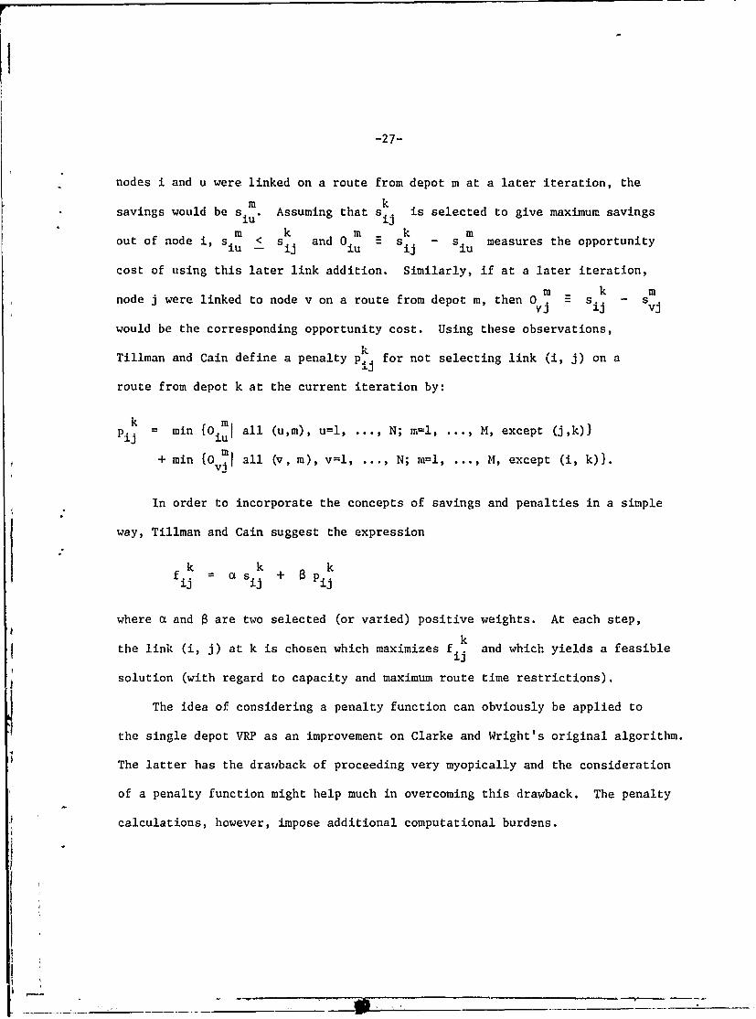
-27-

nodes i and u were linked on a route from depot m at a later iteration, the

m ksavings would be s iu. Assuming that s j is selected to give maximum savings

m k . k mout of node i, Siu < s k and 0 .u k s - Si measures the opportunity

cost of using this later link addition. Similarly, if at a later iteration,

m k mnnode j were linked to node v on a route from depot m, then 0 s k S

V i si vj

would be the corresponding opportunity cost. Using these observations,

Tillman and Cain define a penalty P k for not selecting link (i, j) on a

route from depot k at the current iteration by:

k 0 m

p = ml all (u,m), u=l, ... , N; r=l, ... , M, except (j,k)}Pij mn[ uM xet(~)

+ mi {Oum all (v, m), v=l, ... , N; m=l, ... , M, except (i, k)}.

In order to incorporate the concepts of savings and penalties in a simple

way, Tillman and Cain suggest the expression

k k kai = si +ij ii

where a and 8 are two selected (or varied) positive weights. At each step,

kthe link (i, j) at k is chosen which maximizes f.. and which yields a feasible1]

solution (with regard to capacity and maximum route time restrictions).

The idea of considering a penalty function can obviously be applied to

the single depot VRP as an improvement on Clarke and Wright's original algorithm.

The latter has the drawback of proceeding very myopically and the consideration

of a penalty function might help much in overcoming this drawback. The penalty

calculations, however, impose additional computational burdens.

-28-

VI. ALGORITID I FOR THE MULTI-DEPOT VRP

The algorithm proposed here is based on the savings method, and is

motivated by a desire to find an algorithm capable of handling large size

problems. Algorithm I uses Tillman and Cain's approach for computing savings

but excludes the idea of a penalty function. Our main contribution, at this

stage, is a method of manipulating data which allows fast computation and

minimizes storage requirements.

Algorithm I extends Clarke and Wright's algorithm to the case of many

depots. The idea is to start with an initial solution consisting of each

node being served exclusively by a route from the closest depot. The algorithmk

proceeds by selecting at each step the largest savings s.., computed as in

Tillman and Cain [68], and i and j are linked on a route served from depot k.

Once a link has been created it is never removed in later steps, and the

assignment of nodes i and j to depot k is also final.

In most codes written for the VRP using the savings approach, the problem

of storing the list of savings oen has set the limit on the size of problems

tractable. In the multi-depot VRP, to each depot corresponds a matrix of

savings and the total number of storage locations needed grows quickly

(even though the number of depots is generally small for transportation

networks). In order to cope with the problem of storage, we have used the

following approach.

kFirst, we note that the savings sij associated with the linkage of

nodes i and j at k is symmetric in i and j. We can exploit this symmetry by

stori'g savings in rectangular rather than square matrix form. We perform

LIhe operation illustrated in Figures IV and V. N1 is defined to be N/2 if

-29-

N is even and (N+l)/2 if N is odd (N being the number of demand nodes in

the problem). We replace elements of triangle I by elements of triangle

II, row by row, starting from the last row of triangle II, and in reverse

order. We obtain a rectangular matrix Sk of dimension (N-l) x N1 which

contains all the necessary data. Examples for N even and odd are given in

Figure VI.

1 NI redundant

information

* Ij

Figure IV. Storing savings in a square matrix.

Each element Sk (I, J) of the matrix S corresponds to a savings sijkk k i

which is stored in location (I, J) of Sk according to the following rules:

For N even, Sk (I, J) = +l, J if I > J

SN-l+l, N-J+l if I < J;

sk1+1, J if >

For N odd, Sk (I, J = --

sk

N-I+l, N-J+l if I < J < (N-1)/2

0 if I < J = (N+1)/2.

For large problems, a further economy is achieved by transforming the

ksij into half-word integers, caution being taken against overflow. Round--off

.-30-

o S S ... S ,N .. .. S N I triangle i

HS 2 ,1 NI// s .. 2,N

t3,1 s3,2 -

II1N1,

SI s N,Nl'/ triangle II

Ni

Figure V. Storing savings in rectangular form.

N s 2 1 s7 ,6 S5 0

S 3 ,1 s3 , ..,6,5 0

s4,1 4,2 s4 N

S 5 , 1 s5 ,2 s5, 3 5,

6,1 6,2 6,3 6,4

s7,1 s7,2 s7,3 S7,4

s 1- s sN :8 2,1 N 8 , 7 8,6 8,5

s3, 1 s3, 2 7,6 7,5

s4,1 4,2 s4, 3 . 6,5

sN5,4

S6,4

s7, 4

s 8,1 s8,2 s 8,3 s8,4

Figure VI. Examples of savings matrices.

-31-

* errors can be minimized by first multiplying al real distances by a factor

of 100.

In the computer program, we define ROWIAX(I) as the largest element in

all the rows I of all the M matrices Sk, k=l, ..., M. At each step of the

algorithm, the maximal savings is obtained by searching for the maximum

among the ROWMAX(I), I=, ..., N-1. This can be readily accomplished via

heap structures, as we have noted previously. The main advantage of using

the auxiliary variable ROWM0AX and searching for the maximal savings among

ROWM0AX(I), I=i, ..., N-1 instead of searching directly through the whole

list of savings is an economy of computation time. At each iteration of the

algorithm, we have to update some rows and columns of the savings matrix.

Typically, this operation involves changes only for a few elements of the

vector ROWMAX. Updating the vector ROWMAX and then selecting its largest

element involves much less comparisons than searching through the whole

list of new savings.

Each node is repre3ented by its rectangular coordinates. Four pointers

are associated with each node I: L(I), RT(I), TERM(I), and SQ(I). We

define these below:

2 if I is the only node on a route

L(I) = 1 if I is an endpoint on a route

0 if I is an interior point on a route

RT(I) is the number of the route which contains I

TERM(I) is the terminal to which I is assigned

SQ(I) is the load of the truck which serves I.

The algorithm starts with a solution consisting of each node being exclusively

served by a route from the closest depot and at each subsequent step we link node

-32-

i and j at terminal k in order to realize the largest possible savings.

Steps of Algorithm I

Step 0. L(I) = 2RT(I) = I for I = 1, ..., N.SQ(I) = Q(M)

Step I. For i=l, ... , N, find dit=mjn dik. Set TERM(I) - and MIND(I) = dit

where MIND(I) is the distance from terminal t to demand node i.

Step 2. Compute savings:

k C0 if SQ(I) + SQ(J) > CAP

Ij k ksij 2 MIND(I) + 2 MIND(J) - di - d - d if SQ(I) + SQ(J) < CAP.

Step . Determine ROWMAX(I) for I-1.. ..., N-1, and for each I, determinethe indices KMAX(I) and JMAX(I) such that ROWMAX(I)S (I, J MX(I)).KNAX (I)

Step 4. Compute OPT = Max {ROWMAX(I)II=l, ... , N-li. IOPT is the indexof OPT (i.e., OPT = ROW1*AX(IOPT)). If O T = 0, go to StepIf OPT > 0, trace back to the savings sij which corresponds toOPT as follows:Let JOPT = JMAX(IOPT) and KOPT = KMAX(IOPT).If IOPT > JOPT then i = IOPT + 1,

j = JOPT, and

Here, OPT =S KOPT Lk = KOPT.

IOPT+l, JOPT"

If IOPT < JOPT then i = N - IOPT + 1,j= N - JOPT + 1, and

_K OPTHere, OPT = S KP

N - IOPT + 1, N - JOPT + 1'

Nodes i and j are linked at terminal k.

Step. Update pointers:TERM(I) = TERM(J) = k.L (1) L- L(I) -

L(J) + L(J) -

For all nodes w C RT(1) or RT(J), RT(w) RT(I) andSQ(w) SQ(1) + SQ(J).

DIST - DIST + dij

-33-

ksj 4-O.

Perform Step 6 for h - i and then h = J.

Step 6. If L(h) 1:

set s - 0 for all m#k and all w;k k +2k

sets k shw +2 1 - 2 MIND(h) for allw(#i)

if SQ(h) + SQ(w) < CAP;

set Sk k 0 if SQ(h) + SQ(w) > CAP.hw

If L(h) 0:

set Sm 0 for all m and all w.hw

Step 7. Update ROIWIAX(1) for 1=1, ... , N-1.

Go to Step 4.

Step 8. Compute total distance

N-I

DIST - DIST + Z L(i) . d iTERM(i) and then stop.i=l

Modifications and Improvements

The version of Algorithm I we have described requires the computation of

all savings sij for which Q(i) + Q(j) < CAP at the initialization step. The

Nnumber of computations here can be close to M(). However, it is not necessary

to search through all possible linkages of i to other nodes. It is sufficient

to consider only those nodes which are close neighbors of i. We set up

a grid here as described in a pievious section.

in order to assess the z-onomy of computation brought about by the grid,

we have tried the idea on a problem with 50 nodes and 4 depots: without

using a grid, Algorithm I took 2.04 seconds total CPU time and with a grid,

it took 1.38 seconds while giving the same solution.

As with the single depot VRP a route shape parameter line search has

-3 I -

been studied. In general there seems to be no way a priori to determine

a best value of y for any given problem. The algorithm is fast enough,

however, so that ,we can try different values of y and then selec- the best

solution produced. We have tried the idea on a 50-node, 4-depot problem;

results are given in Table V.

Value Solution produced by algorithmof a

Total distance Number oftraveled routes

.2 584.63 6

.4 559.89 6

.6 512.09 6

.8 509.77 61.0 509.30 71.2 508.07 71.4 518.10 71.6 536.40 111.8 560.40 132.0 587.28 15

Table V. Testing route shape parameter for multi-depot problems.

The advantage of this approach is that we are given a few alternatives

to chose from and depending o-, the objective function, one solution or

another can be selected. For example, in the above illustration, the sole

criterion of minimal distance traveled would determine the choice of

y = 1.2; but the consideration of distance traveled combined with the number

of routes might set the value y .8 as Lhe best choice.

Another positive feature of the method is that after drawing the

different routes produced for different values of y, it is usually possible

to combine some of them manually, simply by examining the various alternatives,

-35-

to produce an even better solution. For example, we worked a few minutes on

the solution obtained with y = 1.0, and obtained a solution with 6 routes

and a total distance traveled of 487 units. We will describe a computer

code which performs a similar refining operation later in this paper.

The above idea is of course a simplistic opplication of the interactive

approach to VRP solving. The appeal of the method is its possibility of

combining extensive and long computations done with a computer with the

intuition and judgement of the human mind. Krolak et. al. [441 have

conducted research in this direction.

Some Computaticnal Results

We have run a program implementing the above ideas for some problems

which were solved by Gillett and Johnson [27]. A version of Algorithm I

which is especially well-suited for problems with an even number of depots

was ised. instead of storing the savings in matricee .f dimension (N-1) x Nl,

we store them in M/2 (M is even) square matrices each N x N; the upper half

of the kth matrix corresponds _o savings associated with depot 2k - 1, and

the lower half corresponds to savings associated with depot 2k. Clearly,

an odd number M of depots ureates no additional snags unless M is large.

This version is slightly faster tCan the original Algorithm I since less

manipulation of indices is involved.

-36-

I 2k-I

S I I ijNi \I I

NI

k "s ij I _ ___ _' 0

Figure VII. Savings matrix for M even.

The code we have written using the above storage scheme is compiled

in 0.18 seconds on an IBM 370/168 and takes 8400 bytes of core. A problem

of 200 nodes and 4 depots necessitates 200k of core memory (using halfword

integers for savings), 300 nodes and 4 depots take 400k, 200 nodes and 10

depots take 420k. We consider these to be medium-sized problems. Results

for some sample problems are summarized in Table VI.

VII. ALGORITHM II: EXTENSION OF ALGORITHM I FOR LARGE PROBLEMS

With larger problems, for example with 1000 nodes, an approach is to

divide the problem into as many subproblems as there are depots and to

solve each subproblem separately. Basically, there are two steps involved

in a multi-depot VRP: first, nodes have to be allocated to depots; then

routes are built which link nodes assigned to the same depot. Ideally, it

is more efficient to deal with the two steps simultaneously, as Algorithm I

does, but the method is no longer computationally tractable when the number

of nodes becomes too large.

-37-

4)MLj 1 '0 ,

CNJ 14 1-q J- O-:j-41 14

$4 2 ae.-r~N0w

~ ~ 4 V)C1

41 U) C4 1 C )

'-1 0)'

E 0 0 -1~~- 1 -4'-'I cN .. . . 4

I 0) 1- 44Z' u C - m 00

,4 000 C Co co -CCCo.Ua ~ - - 0U

4jU 00(-r 0 cq 'Ti-4 i 0-H 0L~~ 0 C% ON C -4 H

>) 0j 0 )

u 4 4-J

C~~00 0 0 0 0 CD * .0 co o (000 0 0 a) 4

H-1eJ Hq H0 1-1 m

-4 C)

*r4 4) .0) 4J w 0~

Q))- 0 0) 0-

o

0) W Q)- >

>." 0~

z -4 C) rl c W cC) ~ ~ ~ C CO 00)00) n p E

Z 04))if ~~- .a)z- 0 Lf4HC0 el 0 U

PL4~) 0 '1

E P 00)-0 4

-38-

The idea behind Algorithm II is that if a given node i is much clo3er

to one depot than any other depot, i will be served from its closest depot.

Mien node i is equidistant from several depots, the assignment of i to a

depot becomes more difficult. For every node i, we determine the closest

depot k1 and the second closest depot k . If the ratio ri = di kl/dik2 is

less than a certain chosen parameter 6 (0 < 6 < 1), we assign i to kl;

in the case r. > 6 we say that node i is a border node. The use of the ratio

ri appears in Gillett and Johnson [27] also.

Clearly, if 6 = 0, all nodes are declared border nodes and if 6 = 1,

all nodes are assigned to their closest depot. For a given problem, we

can fix the number of border nodes as we wish, by varying 6.

The method proceeds as follows. In the first step, we ignore the non-

border nodes and Algorithm I is applied to the set of border nodes. The

algorithm allocates the border nodes to depots and simultaneously builds

segments of routes connecting these nodes. k\t the end of this first step,

all nodes of our problem are assigned to some depot and all border nodes

are linked on some routes. The solution to the VRP is produced depot by

depoc using single depot VRP techniques. The segments of routes which are

built on border nodes are extended to the remaining nodes.

It is felt that the efficiency of the method depends on how many border

nodes Algorithm I can handle. One approach which allows a maximal number

of border nodes to be considered involves the ordering of nodes by decreasing

ratios r. Alternatively, one can experiment with a list of increasing

values of 6. As 6 increases from 0 to I the number of border nodes

decreases. The method described here has been implemented with real data

taken from the distribution information of a local newspaper. The problem,

-39-

with almost 600 nodes and 2 depots, ran in under 55 seconds.

VIII. POST-PROCESSOR

In a previous section we mentioned the possibility of improving the

solution obtained by Algorithm I by modifying the routes that it produced.

In this section, we discuss a computerized procedure to perform this task.

We suppose that initially we are given a solution to Lhe VRP. An

arbitrary orientation is assigned to each route so that for each node i,

we can define pr(i) to be the node or depot which precedes i on its route

and fl(i) to be the node or depot which follows i on its route.

If a node j is inserted between nodes i and fl(i), the reduction in

distance traveled can be computed as:

*ui.= dprj +d. + d, -d - d. .- d.ij pr(j), j j, fl(j) i, fl(i) pr(j), fl(j) 1, j j, fl(i).

To any pair of nodes i and j, we can consider the savings u.. corresponding

to the insertion of node j between i and fl(i). In addition, if node i

is the first node served by a route, then the savings vii associated with

the insertion of node j between i and pr(i) has to be taken into account.

If the number of routes is r, then the possible savings can be stored in

a rectangular matrix W of dimension (N + r) x N. The first N rows correspond

to savings u and the last r rows refer to the savings vi. We note that

in general w.. # w...

The post-processor searches for the largest element of W which is

feasible, and performs the indicated insertion. The operation is then repeated

until no further reduction in total distance traveled is possible. The details

-40-

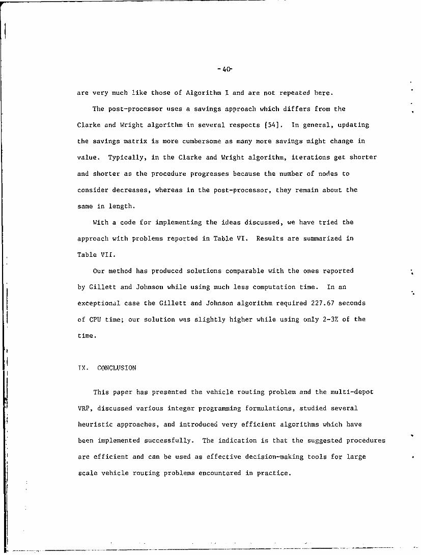
are very much like those of Algorithm I and are not repeated here.

The post-processor uses a savings approach which differs from the

Clarke and Wright algorithm in several respects [54]. In general, updating

the savings matrix is more cumbersome as many more savings might change in

value. Typically, in the Clarke and Wright algorithm, iterations get shorter

and shorter as the procedure progresses because the number of nodes to

consider decreases, whereas in the post-processor, they remain about the

same in length.

With a code for implementing the ideas discussed, we have tried the

approach with problems reported in Table VI. Results are summarized in

Table VII.

Our method has produced solutions comparable with the ones reported

by Gillett and Johnson while using much less computation time. In an

exceptional case the Gillett and Johnson algorithm required 227.67 seconds

of CPU time; our solution was slightly higher while using only 2-3% of the

time.

TX. CONCLUSION

This paper has presented the vehicle routing problem and the multi-depot

VRP, discussed various integer programming formulations, studied several

heuristic approaches, and introduced very efficient algorithms which have

been implemented successfully. The indication is that the suggested procedures

are efficient and can be used as effective decision-making tools for large

scale vehicle routing problems encountered in practice.

u__ __ _ IT ___ ______ __ -41

$40to-4 c< 0

:t 0(700k t- n

Q) 0

20

0. 1-4C.; r 1 -4

rz (7 O-4 0 r-O0

0 (0 0

0$44

2o~to

(00 a

Q) 0)0

0 0

$4 *HJ0

I -H ) JnCqLf" Ln Lf

(0 w r.0 q Li r- $4l 0\0O\.4 IN0r

0

4-i

u ~ 00) 0-

0) (0 0 - r4

04-~. C'J0-( Cl 0 -Ic

C)i 0

$4 140 C 14-Ti0 %0L -

0$4

-42-

REFERENCES

1. Agin, N., and Cullen, D., "An Algorithm for Transportation Routing andVehicle Loading," Management Science, Special Issue an Logistics, 1975.

2. Altman, S., Bhagat, N., and Bodin, L., "Extension of the Clarke an~hWright Algorithm for Routing Garbage Trucks," Presented at the 18TIMS Int. Cont. (Washington, D.C.) March 1971.

3. Angel, R., Caudle, R., and Whinston, A., "Computer Assisted SchoolBus Scheduling," Management Science, Vol. 18, No. 6, Feb. 1972, p. 279.

4. Balinski, M., and Quandt, R., "On an Integer Program for a DeliveryProblem," Operations Research, Vol. 12, No. 2, 1964, pp. 300-304.

5. Bellmore, M., and Hong, S., "Transformation of Multisalesmen Problemto the Standard Traveling Salesman Problem," JACM, Vol. 21, No. 3,July 1974, pp. 500-504.

6. Bellmore, M., and Nemhauser, G., "The Traveling Salesman Problem:A Survey," Operations Research (1968), Vol. 16, pp. 538-558.

7. Beltrami, E., and Bodin, L., "Networks and Vehicle Routing for MunicipalWaste Collection," Networks, Vol. 4, No. 1, 1974, pp. 65-94.

8. Bennett, B., and Gazis, D., "School Bus Routing by Computer," Transporta-tion Research, Vol. 6, No. 4, Dec. 1972, pp. 317-325.

9. Biles, W., and Bradford, J., "A Heuristic Approach to Vehicle Schedulingwith Due-Date Constraints," Presented at the 1975 Chicago ORSA meeting,May 1975.

10. Bodin, L., "A Taxonomic Structure for Vehicle Routing and SchedulingProblems," Comput. and Urban Soc., Vol. 1, pp. 11-29, 1975.

1i. Bodin, L., and Berman, L., "Routing and Scheduling of School Busesby Computers," Presented at Fall 1974 ORSA meeting in San Juan.

12. Boekemeier, R., "An Operationalto]ution of a Large Scale DeliveryProblem," mimeo presented at 27 National ORSA meeting, Boston, Mass.,May 1965.

13. Cassidy, P., and Bennett, H., "TRAMP - A Multi-depot Vehicle SchedulingSystem," Operational Research Quarterly, Vol. 23, No. 2, pp. 151-163.

14. Chard, R., "An Example of an Integrated Man-Machine System for TruckScheduling," Operational Research Quarterly, Vol. 19, 1968, p. 108.

15. Christofides, W., and Eilon, S., "An Algorithm for the Vehicle DispatchingProblem," Operational Research Quarterly, Vol. 20, 1969, p. 309.

-43-

16. Christofides, N., and Eilon, S., "Algorithms for Large Scale TSP's,"Operational Research Quarterly, Vol. 23, 1972, p. 511.

17. Christofides, N., "The Vehicle Routing Problem," July 1974, NATOConference on Combinatorial Optimization, Paris.

18. Clarke, G., and Wright, J., "Scheduling Of Vehicles from a CentralDepot to a Number of Delivery Points," Operations Research, Vol. 12,No. 4, 1964, pp. 568-581.

19. Cochran, H., "Optimization of a Carrier Routing Problem," unpublishedM.S. Thesis, Industrial Engineering Dept., Kansas State University, 1967.

20. Dantzi3, G., and Ramser, J., "The Truck Dispatching Problem," Management

Science, October 1959, pp. 81-91.

21. Eilon, S., Watson-Gandy, C., and Christofides, N., Distribution Management,Griffin, London, 1971.

22. Ferebee, J., "Controlling Fixed-Route Operations," Industrial Engineering,Vol. 6, No. 10, Oct. 1974, pp. 28-31.

23. Floyd, R., "Treesort Algorithm 113," ACM Collected Algorithms, August 1962.

24. Gabbay, H., "An Overview of Vehicular Scheduling Problems," M.I.T.Operations Research Center Technical Report, No. 103, Sept. 1974.

25. Garvin, W., Crandall, H., John, J., and Spellman, R., "Applicationsof Linear Programming in the Oil Industry," Management Science, Vol. 3,No. 4, July 1957, pp. 407-430.

26. Gaskell, T., "Bases for Vehicle Fleet Scheduling," Operational ResearchQuarterly, Vol. 18, 1967, p. 281.

27. Gillett, B., and Johnson, J., "Sweep Algorithm for the Multiple DepotVehicle Dispatch Problem," presented at the URSA/TIMS meeting San Juan,Puerto Rico, Oct. 1974.

28. Gillett, B., and Miller, L., "A Heuristic Algorithm for the VehicleDispatch Problem," Operations Research, Vol. 22, 1974, p. 340.

29. Golden, B., "Vehicle Routing Problems: Formulations and HeuristicSolution Techniques," M.I.T. Technical Report, Operations Research Center,

No. 113, August 1975.

30. Hausman, W., and Gilmour, P., "A Multi-Period Truck Delivery Problem,"Transportation Research, Vol. 1, 1967, pp. 349-357.

31. Hays, R., "The Delivery Problem," Carnegie Inst. of Tech., ManagementScience Research Report No. 106, 1967.

- -- - - - - - - - - - ---__

-44-

32. Held, M., and Karp, R., "The Traveling-Salesman Problem and MinimumSpanning Trees," Operations Research, Vol. 18, No. 6, 1970, pp. 1138-1162.

33. Held, M., and Karp, R., "The Traveling-Salesman Problem and MinimumSpanning Trees, Part 7I," i-athematical Programming, Vol. 1, No. 1,1971, pp. 6-25.

34. Holden, N., "The School Transportation Problem," Doctoral Thesisin Business Administration, Indiana University, 1967.

35. Hudson, J., Grossman, D., and Marks, D., "Analysis Models for SolidWaste Collection," M.I.T. Civil Engineering Report, Sept. 1973.

36. IBM Corp., "Systcm 360/Vehicle Scheduling Program Application Description -VSP," Report 1120-0464, White Plains, N.Y., 1968.

37. Jirvinen, P., "On a Routing Problem in a Graph with Two Types of CostsAssociated with the Edges," Acta Universitatis Tamperensis, Ser. A,Vol. 50, 1973.

38. Karg, L., and Thompson, G., "A Heuristic Approach to Solving TravelingSalesman Problems," Management Science, Vol. 10, pp. 225-248.

39. Kershenbaum, A., and Van Slyke, R., "Computing Minimum Spanning TreesEfficiently," Proceedings of 1972 ACM Conference, Boston, August, 1972.

40. Kirby, R., and MacDonald, J., "The Savings Method for Vehicle Scheduling,"Operational Research Quarterly, Vol. 24, No. 2, June 1973, p. 305.

41. Klincewicz, J., "The Tyagi Algorithm for Truck Dispatching," UROPFinal Project Report, M.I.T., 1975.

42. Knight, K., and Hafer, J., "Vehicle Scheduling with Timed and ConnectedCalls: A Case Study," Operational Research Quarterly, Vol. 19, No. 3,Sept. 1968, p. 299.

43. Knowles, K., "The Use of a Heuristic Tree Search Algorithm for VehicleRouting and Scheduling," Lecture at OR conference, Exeter, England, 1967.

44. Krolak, P., Felts, W., and Nelson, J., "A Man-Machine Approach towardSolving the Generalized Truck Dispatching Problem," Transportation Science,Vol. 6, No. 2, 1972.

45. Lam, T., "Comments on a Heuristic Algorithm for the Multiple TerminalDelivery Problem," Transportation Science, Vol. 4, No. 4, Nov. 1970, p. 403.

46. Lin, S., "Computer Solutions of the TSP," Bell Systems Technical Journal,Vol. 44, 1965, p. 2245.

47. Lin, S., and Kernighan, B., "An Effective Heuristic Algorithm for the TSP,"Operations Research, Vol. 21, 1973, p. 498.

-45-

48. Little, J.D.C. , Murty, K., Sweeney, D., and Karel, C., "An Algorithmfor the Traveling Salesman Problem," Operations Research, Vol. 11, No. 6,1963, pp. 972-989.

* 49. MacDonald, J., "Vehicle Scheduling - A Case Study," Operational ResearchQuarterly, Vol. 23, No. 4, 1972, pp. 433-444.

50. Maffei, R., "Modern 1,ethods for Local Delivery Route Design," Journal ofMarketing, Vol. 29, April 1965, pp. 13-18.

51. Miller, C., Tucker, A., and Zemlin, R., "Integer Programming Formulationof Traveling Salesman Problems," JACM, 7, (1960), pp. 326-329.

52. Nace, G., "Distributing Goods by VSP/360," Software Age, Vol. 3, No. 3,March 1969, p. 8.

53. Newton, R., and Thomas, W., "Design of School Bus Routes by DigitalComputer," Socio-Economic Plan. Science, Vol. 3, 1969.

54. Nguyen, H., "Multi-Depot Vehicle Routing Problems," Masters Thesis,Sloan School of Management, M.I.T., 1975.

55. Noonan, R., and Whinston, A., "An Information System for Vehicle Scheduling,"Software Age, Vol. 3, No. 12, Dec. 1969, p. 8.

56. O'Brien, H., "A Redefinition of Savings," Operational Research Quarterly,Vol. 20, 1969.

57. Orloff, C., "A Fundamental Problem in Vehicle Routing," Networks, Vol. 4,No. 1, pp. 35-64, 1974.

58. Orloff, C., "Routing a Flee±t of M Vehicles to/from a Central Facility,"Networks, Vol. 4, pp. 147-162.

9q. Pierce. J., "Direct Search Algorithms for Truck-Dispatching Problems,Part I," Transportation Research, Vol. 3, pp. 1-42.

60. Russell, R., "Efficient Truck Routing for Industrial Refuse Collection,"presented at the ORSA/TIMS meeting San Juan, Puerto Rico, Oct. 1974.

61. Saha, J., "An Algorithm for Bus Scheduling Problems," OperationalResearch Quarterly, Vol. 21, No. 4, 1970, pp. 463-474.

62. Schruben, L., and Clifton, R., "Routing Delivery Trucks - Case Studies,"mimeo paper presented at ORSA/TIMS meeting, San Francisco, California,May 1968.

63. Scott, A., Combinatorial Programming, Spatial Analysis and Planning,

Methuen & Co. Ltd., London, 1971.

64. Shapiro, D., "Algorithms for the Solution of the Optimal Cost TravellingSalesman Problem," Sc. D. Thesis, Washington University, St. Louis, 1966.

-46-

65. Svestka, J., and Huckfeldt, V., "Computational Experience with anM - Salesmen Traveling Salesman Algorithm," Management Science, Vol. 19,No. 7, 1973, pp. 790-799.

66. Tillman, F., "The Author's Reply to Uebe's Note," Transportation Science,Vol. 4, No. 2, May 1970, p. 232.

67. Tillman, F., "The Multiple Terminal Delivery Problem with ProbabilisticDemands," Transportation Science, Vol. 3, No. 3, August 1969, p. 192.

68. Tillman, F., and Cain, T., "An Upper Bounding Algorithm for the Singleand Multiple Tenminal Delivery Problem," Management Science, Vol. 18,No. 11, 1972, pp. 664-682.

(9. Tillman, F., and Cochran, H., "A Heuristic Approach for Solving theDelivery Problem," J. Indust. Eng., Vol. 19, 1968, p. 354.

70. Tracz, G., and Norman, M., "A Computerized System for School Bus Routing,"Ontario Institute for Studies in Education, Toronto 181, Ontario, 1970.

71. Turner, W., Ghare, P., and Fourds, L., "Tr;nsportation Routing Problem -A Survey," AIIE Transactions, Vol. 6, No. 4, Dec. 1974, pp. 288-301.

72. Tyagi, M., "A Practical Method for The Truck Dispatching Problem,"Journal of the Operations Research Society of Japan, Vol. 10, pp. 76-92.

73. Uebe, G., "Comments on Tillman's Paper," Transportation Science, Vol. 4,No. 2, May 1970, p. 226.

74. Unwin, E., "Bases For Vehicle Fleet Scheduling," Operational ResearchQuarterly, Vol. 19, No. 2, June 1968, p. 201.

75. Webb, M., "Relative Performance of Some Sequential Methods of PlanningMultiple Delivery Journeys," Operational Research Quarterly, Vol. 23,No. 3, pp. 361-372, 1.972.

76. Webb, M., "The Savings Method for Vehicle Scheduling - A Reply,"Operational Research Quarterly, Vol. 24, No. 2, June 1973, p. 307.

77. Williams, J., "Algorithm 232: Heapsort," Corm. ACM, Vol. 7, No. 6,pp. 347-348, 1964.

78. Wilson, N., Sussman, J., Wong, H., and Higonnet, T., "SchedulingAlgorithms for a Dial-A-Ride System," Report USL TR-70-13, Urban SystemsLaboratory, M.I.T., March 1971.

79. Wren, A., and Holliday, A., "Computer Scheduling of Vehicles from Oneor More Depots to a Number of Delivery Points," Operational ResearchQuarterly. 23, pp. 333-344 (1972).

80. Yellow, P., "A Computational Modification to the Savings Method of

Vehicle Scheduling," Operational Research Quarterly, Vol. 21, 1970, p. 281.