Implementing the speed layer in a lambda architecture -...

Implementing the speed layerin a lambda architecture

IT4BI MSc Thesis

Student: ERICA BERTUGLIAdvisor: FERRAN GALI RENIU (TROVIT)

Supervisor: OSCAR ROMERO MORAL

Master on Information Technologies for Business IntelligenceUniversitat Politecnica de Catalunya

BarcelonaJuly 31, 2016

A thesis presented by ERICA BERTUGLIin partial fulfillment of the requirements for the MSc degree on

Information Technologies for Business Intelligence

Abstract

With the increasing growth of big data and the necessity of near real-time analysis, it appeared the re-quirement of a solution able to conciliate existing ETL batch processing methods with newly developedstream-processing methodologies designed to obtain a view of online data.Lambda architecture [1] is the data-processing architecture that enables the possibility of exploiting bothbatch- and stream-processing methods in the attempt of balancing latency, throughput, and accuracy.The project aims to demonstrate how lambda architecture can be a good approach for a company to enablenear real-time analytics integrating the existing batch processes with a streaming solution.

ii

Contents

List of Figures v

List of Tables vi

1 Introduction 11.1 Structure of the work . . . . . . . . . . . . . . . . . . . . . . . . . . . . . . . . . . . . . . 1

2 Current solution 22.1 Data storage . . . . . . . . . . . . . . . . . . . . . . . . . . . . . . . . . . . . . . . . . . . 3

2.1.1 Batch view . . . . . . . . . . . . . . . . . . . . . . . . . . . . . . . . . . . . . . . 32.1.2 Data warehouse . . . . . . . . . . . . . . . . . . . . . . . . . . . . . . . . . . . . . 4

2.2 Data flow . . . . . . . . . . . . . . . . . . . . . . . . . . . . . . . . . . . . . . . . . . . . 42.3 Limitations of the current solution . . . . . . . . . . . . . . . . . . . . . . . . . . . . . . . 6

3 Related work 7

4 Design of the solution 94.1 Requirements . . . . . . . . . . . . . . . . . . . . . . . . . . . . . . . . . . . . . . . . . . 94.2 Architecture . . . . . . . . . . . . . . . . . . . . . . . . . . . . . . . . . . . . . . . . . . . 94.3 Messaging system . . . . . . . . . . . . . . . . . . . . . . . . . . . . . . . . . . . . . . . . 94.4 Speed layer . . . . . . . . . . . . . . . . . . . . . . . . . . . . . . . . . . . . . . . . . . . 114.5 Batch layer . . . . . . . . . . . . . . . . . . . . . . . . . . . . . . . . . . . . . . . . . . . 114.6 Serving layer . . . . . . . . . . . . . . . . . . . . . . . . . . . . . . . . . . . . . . . . . . 12

5 Implementation 135.1 Speed Layer . . . . . . . . . . . . . . . . . . . . . . . . . . . . . . . . . . . . . . . . . . . 13

5.1.1 Technology . . . . . . . . . . . . . . . . . . . . . . . . . . . . . . . . . . . . . . . 135.1.2 Design . . . . . . . . . . . . . . . . . . . . . . . . . . . . . . . . . . . . . . . . . 145.1.3 Invalid clicks detection . . . . . . . . . . . . . . . . . . . . . . . . . . . . . . . . . 15

5.2 Serving layer . . . . . . . . . . . . . . . . . . . . . . . . . . . . . . . . . . . . . . . . . . 165.2.1 Synchronization . . . . . . . . . . . . . . . . . . . . . . . . . . . . . . . . . . . . 165.2.2 Dump of the materialized views in the data warehouse . . . . . . . . . . . . . . . . 16

5.3 Exception handling . . . . . . . . . . . . . . . . . . . . . . . . . . . . . . . . . . . . . . . 175.3.1 Non-blocking exceptions . . . . . . . . . . . . . . . . . . . . . . . . . . . . . . . . 175.3.2 Blocking exceptions . . . . . . . . . . . . . . . . . . . . . . . . . . . . . . . . . . 17

5.4 Fault-tolerance . . . . . . . . . . . . . . . . . . . . . . . . . . . . . . . . . . . . . . . . . 185.5 Monitoring and guarantee of satisfaction of the requirements . . . . . . . . . . . . . . . . . 18

iii

6 Experiments and discussion 196.1 Speed layer . . . . . . . . . . . . . . . . . . . . . . . . . . . . . . . . . . . . . . . . . . . 196.2 Serving layer . . . . . . . . . . . . . . . . . . . . . . . . . . . . . . . . . . . . . . . . . . 216.3 Experiment results . . . . . . . . . . . . . . . . . . . . . . . . . . . . . . . . . . . . . . . 22

6.3.1 Interest of the user . . . . . . . . . . . . . . . . . . . . . . . . . . . . . . . . . . . 256.3.2 Comparison with current solution . . . . . . . . . . . . . . . . . . . . . . . . . . . 25

7 Conclusion and future work 27

Appendices 29

A Logline 30

B Agile Methodology 32

C Additional views for the data warehouse 35

D Survey 37D.1 First survey . . . . . . . . . . . . . . . . . . . . . . . . . . . . . . . . . . . . . . . . . . . 37D.2 Second survey . . . . . . . . . . . . . . . . . . . . . . . . . . . . . . . . . . . . . . . . . . 37

References 38

iv

List of Figures

2.1 UML Class Diagram of loglines. . . . . . . . . . . . . . . . . . . . . . . . . . . . . . . . . 32.2 Current solution. . . . . . . . . . . . . . . . . . . . . . . . . . . . . . . . . . . . . . . . . 32.3 Batch flow 1. . . . . . . . . . . . . . . . . . . . . . . . . . . . . . . . . . . . . . . . . . . 52.4 Batch flow 2. . . . . . . . . . . . . . . . . . . . . . . . . . . . . . . . . . . . . . . . . . . 5

3.1 Lambda architecture from a high-level perspective [8]. . . . . . . . . . . . . . . . . . . . . 73.2 Frameworks benchmarking (figure from [9]). . . . . . . . . . . . . . . . . . . . . . . . . . 8

4.1 Architecture proposed. . . . . . . . . . . . . . . . . . . . . . . . . . . . . . . . . . . . . . 114.2 Sync view in the serving layer . . . . . . . . . . . . . . . . . . . . . . . . . . . . . . . . . . 12

5.1 BPMN of the speed layer. . . . . . . . . . . . . . . . . . . . . . . . . . . . . . . . . . . . . 145.2 Stateful transformation for invalid clicks detection. . . . . . . . . . . . . . . . . . . . . . . 155.3 BPMN of the serving layer. . . . . . . . . . . . . . . . . . . . . . . . . . . . . . . . . . . . 17

6.1 Speed layer: experiments with ad impression loglines . . . . . . . . . . . . . . . . . . . . . 196.2 Ad impressions - Adding cores. . . . . . . . . . . . . . . . . . . . . . . . . . . . . . . . . . 206.3 Ad impressions -Adding executors. . . . . . . . . . . . . . . . . . . . . . . . . . . . . . . . 206.4 Speed layer: experiments with click loglines. . . . . . . . . . . . . . . . . . . . . . . . . . 206.5 Clicks - Adding executors. . . . . . . . . . . . . . . . . . . . . . . . . . . . . . . . . . . . 216.6 Clicks - Adding memory. . . . . . . . . . . . . . . . . . . . . . . . . . . . . . . . . . . . . 216.7 Experiments with view source revenues . . . . . . . . . . . . . . . . . . . . . . . . . . . . 226.8 View source revenues - adding cores . . . . . . . . . . . . . . . . . . . . . . . . . . . . . . 226.9 View source revenues - adding memory . . . . . . . . . . . . . . . . . . . . . . . . . . . . 226.10 View source revenues - adding executors . . . . . . . . . . . . . . . . . . . . . . . . . . . . 22

B.1 Weekly sprints. . . . . . . . . . . . . . . . . . . . . . . . . . . . . . . . . . . . . . . . . . 33B.2 Product backlog. . . . . . . . . . . . . . . . . . . . . . . . . . . . . . . . . . . . . . . . . 34

C.1 Experiments view hit zone monthly . . . . . . . . . . . . . . . . . . . . . . . . . . . . . . 35C.2 Experiments view source revenues hourly . . . . . . . . . . . . . . . . . . . . . . . . . . . 36

v

List of Tables

2.1 Characteristics of the data . . . . . . . . . . . . . . . . . . . . . . . . . . . . . . . . . . . . 42.2 Characteristic of the data flow . . . . . . . . . . . . . . . . . . . . . . . . . . . . . . . . . 6

4.1 Project requirements . . . . . . . . . . . . . . . . . . . . . . . . . . . . . . . . . . . . . . 10

6.1 Experiment results . . . . . . . . . . . . . . . . . . . . . . . . . . . . . . . . . . . . . . . 246.2 Comparison of the logline injection . . . . . . . . . . . . . . . . . . . . . . . . . . . . . . 266.3 Comparison of the serving layer . . . . . . . . . . . . . . . . . . . . . . . . . . . . . . . . 26

vi

Chapter 1

Introduction

The company hosting the Master Thesis, Trovit [2], was founded in 2006 and have headquarters in Barcelona.Trovit is a vertical search engine for classified ads, specialized in four verticals: jobs, cars, real-estates andproducts. The search engine is currently available in 46 different countries, it has 140 million of indexedads and more than 93 million visits per month. The aim of the website is to make available to its users allthe ads available in the web, aggregating several sources. Users can search the ads, refine the result usingfilters, set up regular email alerts, or set up notifications in the mobile app. Ads displayed to the user arecrawled from websites or directly obtained through partnerships with the sources.Trovit business model is based on the following elements:

• pay per click: the partner website pays each time a user clicks on its ad (and is consequently redirectto the source website);• pay per conversion: Trovit is paid each time that a click is converted to a concrete action in the partner

website, for example a contact request;• Google AdSense: Trovit is paid for each advertisements displayed using AdSense technology;• web banners: additional space for advertisements in third websites is sold to partner websites.

For this reason, it is extremely important for the company to always have accurate and current data aboutthe clicks, the impressions, and all the events generated on the website and on the mobile application to beable to correctly monetize them.

1.1 Structure of the work

The following chapters will describe the solution already existing in the company (Chapter 2) and the relatedwork (Chapter 3). Chapter 4 will introduce the requirements of the project as well as the solution proposedwith its architecture. Chapter 5 will detail the implementation while Chapter 6 will describe and discuss theexperiments performed. Lastly, Chapter 7 will present the conclusions of the work.

1

Chapter 2

Current solution

Currently Trovit has an ETL flow that processes the events coming from the web to produce internal statis-tics. The data involved are generically named loglines and are related to the analysis of the usage of thecompany website as well as the mobile application and the alerts. Alerts are emails that are requested bythe user in order to stay updated with new ads of interest. The process involves 15 ETL flows that processrespectively 15 different types of loglines. The following are the type of events analyzed:

• ad impression: every impression in Trovit web pages.• click: when a user goes to a partner’s website through Trovit.• internal click: clicks whose destination is Trovit itself (not the one monetized).• conversion tracking: information about clicks that have been converted to a concrete action on the

partner website.• banner impression: every banner Trovit shows on foreign websites.• alert creation impression: every popup where a user is offered to create an alert.• alert creation: every alert creation or modification.• alert sending: the event of sending a specific alert to a specific user.• alert opening: event generated when a user opens an alert.• api: every use of Trovit API.• api error: every error generated by Trovit API.• app installation status: information about installation or uninstallation of Trovit mobile app.• app push status: settings of the notifications in a mobile app.• app push send: every notification sent through the mobile app.• app push open: every notification that has been opened by the user.

Figure 2.1 show the UML class diagram representing the loglines where in green are the conceptual macro-types of loglines, and in yellow are the types of loglines actually implemented. The existing ETL performsthe following steps:

• reads the loglines from a messaging system (Apache Kafka);• performs a cleaning process and then stores the loglines in a data storage named batch view;• performs aggregations and stores materialized views in a data warehouse.

We name the first data storage as batch view because it doesn’t contain pure raw data but data that havealready been cleaned and de-duplicated, but that are not aggregated.

The architecture of the current solution is shown in figure 2.2. Data analysts can query the non-pre-aggregated data from the batch view or the aggregated data from the data warehouse, moreover they canaccess dashboards built on the data stored in the data warehouse.

2

CHAPTER 2. CURRENT SOLUTION 3

Figure 2.1: UML Class Diagram of loglines.

Figure 2.2: Current solution.

2.1 Data storage

Table 2.1 represents the different characteristic of the data stored in the batch view and in the data warehouse.

2.1.1 Batch view

The batch view has been built using Apache HDFS and it stores Apache Parquet files, used for quick accessto the original data with SQL-like queries through tools like Hive and Impala.

Parquet is an efficient column-oriented binary format designed for Apache Hadoop. Compared to otherformats like Sequence Files or Apache Avro, that are row-based, Apache Parquet is more efficient whenspecific columns are queried and few joins are performed [3]. This is the reason why it has been chosen asformat for the batch view, where the loglines stored have several columns and most of the queries performedselect only few columns and are focused on one type of logline (thus no joins are performed). Moreover,Parquet allows efficient compression of the data. Another format that would be efficient for Trovit use caseis Apache ORC (Optimized Row Columnar), however this is not fully supported by Cloudera Impala, aquery engine used by Trovit alternatively to Apache Hive, and additionally there are tests benchmarkingORC and Parquet that demonstrate that Parquet is more efficient [4]. However, to effectively choose the bestformat, in the future, new empirical tests should be performed, but this goes beyond the scope of this thesis.

Data stored in Parquet are made available to the user through Apache Hive and in particular with thecreation of partitioned external tables. Since most of the queries performed on the batch view analyzes data


Characteristic Batch view Data warehouse

Granularity LoglineDifferent granularities in different views(Day or month, vertical, country, etc)

Format of the data Parquet Relational tablesData storage Apache HDFS MySQLHistoricity (= range of data stored) Since ever Since everData freshness (= time interval betweenwhen the data are produced and whenthey are inserted in the data storage)

1 hour and 30 minutes(approximatively)

1 hour and 40 minutes(approximatively)

How data are accessedApache Hive queries,Cloudera Impala queries

Sql queries, reporting tools

Table 2.1: Characteristics of the data

of few days or few months, tables are partitioned by day to allow fast queries avoiding full table scans. Infact, all the queries performed with Hive always filter on the partition, named s datestamp, using the formatSELECT col i1, col i2, . . . , col ik FROM table name WHERE s datestamp IN (day1, day2, . . . , dayn)AND additional filters. An example of the Parquet format for the logline click has been provided in theappendix A.

2.1.2 Data warehouse

The data warehouse is implemented on a relational database. The concept of data warehouse developed inTrovit is a set of several materialized views of aggregated data, analyzed through SQL queries. Currentlythe data warehouse consists of 41 tables, considering only the ones displaying internal statistics and createdthrough the aggregation of the 15 Hive external tables previously mentioned. Because of the slow readperformances of the relational database, expensive SQL operations between the different tables are tryingto be avoided, thus every time that new analysis are required and are forecasted to be performed quite oftennew tables are created or the old ones are updated. This is done with the awareness that a relational databaseis not best choice for the implementation of Trovit data warehouse and that in the future a new solution willbe designed. Similarly, the concept of a data warehouse as a set of materialized views may in the futurebe substituted by a multidimensional model that would enable OLAP queries. A detailed study would beneeded to analyze the limitations of using a relation database for Trovit data warehouse and the possiblealternatives. However some evident limitations of using MySql as data warehouse are the following:

• it cannot scale out;• it performs slow writings if compared with some distributed storage systems;• it cannot handle concurrent writings and readings.

Generally the tables available in the data warehouse have a granularity of one day, one vertical and onecountry. Some of the tables also have other levels of granularity, for example a source, that is a specificwebsite from which ads are taken.

2.2 Data flow

The ETL process consists of two sequential batch flows, this is due to a rearrangement of an old batchflow previously existing in Trovit. The first flow, represented in figure 2.3, is executed every 15 minutes, it


collects the loglines from Apache Kafka, it transforms them in JSON format and stores them in a temporarystorage from where data will be read by the second flow. The temporary storage is located in Apache HDFS.The second flow (figure 2.4) is executed every hour and performs the following steps:

1. Reading the loglines from the temporary storage.

2. De-duplicating the loglines read and splitting them in small files, assuring that no loglines from twodifferent days are in the same file.

3. Compacting the loglines per day and performing some additional logic to add information to the finalstatistics (invalid click detection and out of budget detection).

4. Storing the data in the batch view. During this phase a new partition with the daily loglines is addedto the related Hive external tables.

5. Aggregating the loglines per day and storing them in the data warehouse (overwriting the valueswritten with the previous batch processes for the same day).

Figure 2.3: Batch flow 1.

Figure 2.4: Batch flow 2.

Steps 2,3 and 4 are MapReduce jobs and read from HDFS, thus each of these steps stores data intodisk twice, once after the map phase and one after the reduce phase. Step 5 uses Apache Sqoop, a toolable to perform the data transfers between HDFS and MySql. Sqoop is the most common tool used totransfer data from HDFS to a structured database, however the internal implementation of Sqoop, based onMapReduce jobs, may be a bottleneck for the application because data are stored on disk after each mapand reduce operation. The batch process as described above makes data available on MySql with a delay


Characteristic Data FlowETL Latency (= the time interval between the beginningof the process and the update of the data warehouse)

Approx. 30 minutes

Data freshness (= the time interval between when the dataare produced and when they are inserted in the data warehouse)

Approx. 1 hour and 40 minutes

TechnologyApache Hadoop Map Reduce,Apache Sqoop

ModularityThe ETL process is able to handlethe different types of loglines.

Table 2.2: Characteristic of the data flow

of approximately one hour and 40 minutes, due to the scheduled delay of the first flow (15 minutes) and ofthe second flow (one hour) and to the execution time of the full flow (approximately 30 minutes). Table 2.2shows the characteristics of the data flow.

2.3 Limitations of the current solution

The main limitation of the process currently in place in Trovit is that both the batch view and the datawarehouse are updated approximately every one hour and 30 minutes. This is mainly due to the fact thatthe whole process is implemented with Apache Hadoop MapReduce, whose bottleneck is the writing todisk after each phase. For this reason Trovit decided to explore a solution that could enable near real-timeanalytics, in particular with the following motivations:

• to allow data analysts to react on time to possible business changes;• to allow developers to have an immediate overview of the results of changes made to the processes,

correcting possible bugs with small delay and activating automatic monitoring based on online data;• to automate processes of decision making that help the company to better monetize the clicks received

according to the clicks registered until that moment.

Regarding the last point it is important to notice that one of the source of revenue for Trovit is thatpartner websites pay each time a user click on one of their ads. However the partners agree with Trovit for adaily budget that they are willing to pay. For this reason its important to be able to detect almost on real-timewhen a partner has already ended its daily budget, and to do that to be able to detect which clicks must beinvoiced (valid) and which not. Currently Trovit calculates this information every hour with the batch flow,having this information in near-real time would allow to detect immediately which source website do nothave any budget left and to automatically “favor” in the result page the ones that still have budget.

Chapter 3

Related work

In the past different architectures have been studied to enable real-time analytics. However most of thesolutions proposed (e.g. fully incremental architecture described in [5], Kappa architecture [6] and Zetaarchitecture [7]) have been discarded in favor of the lambda architecture, that is currently the most commonlyadopted. Lambda architecture [1] is the data-processing architecture that enables the possibility of exploitingboth batch- and stream-processing methods in the attempt of balancing latency, throughput, and accuracy.It is an architecture design where a sequence of records is fed into a batch system (named batch layer) and astream processing system (named speed layer) in parallel, as shown in figure 3.1. The logic in the two layers

Figure 3.1: Lambda architecture from a high-level perspective [8].

may be slightly different because each layer aims to satisfy specific requirements. The batch layer managesthe master dataset (an immutable, append-only set of raw data) and continuously creates batch views of thedata. This is a high-latency operation, because its running a function on all the data, and by the time thebatch layer finishes, a lot of new data will have collected that is not represented in the batch views. For thisreason while batch views are executed, the speed layer takes care of creating real-time views of the datareceived in the meanwhile. The results are merged together in a phase named serving layer, where the actualoutput for the user is produced.Although many companies are currently using or implementing lambda architectures, it is quite difficult tofind details about the design of their systems. For this reason, this section will be focused on the technologiesavailable to implement the system. While the batch layer already exists and is implemented using HadoopMapReduce, for the speed layer and serving layer the technologies have been chosen by the company andare respectively Apache Spark Streaming for the first and Aache Spark for the second. However this section

7

CHAPTER 3. RELATED WORK 8

will give an overview of the main technologies used for use cases with similar requirements. For the speedlayer several streaming technologies are available. The most common are currently Apache Storm, ApacheSpark and Apache Flink. Trovit decided not to use Storm because of the bugs and difficulties encounteredwhen setting up and running other applications with this technology and because it is not developing rapidly,in comparison with Spark and Flink that costantly have new releases and improvements. Moreover Stormdoesn’t provide a framework for batch processing so to choose it would have implied to deal with a secondtechnology for the serving layer. With respect to Spark and Flink, the first has been chosen mostly becausemore mature and because of the support available. More detailed about the comparison between Spark andFlink are available at section 5.1.1.For the serving layer the candidate technologies were several: Hadoop MapReduce, Spark, Metis, and otherframeworks available for batch processing. While MapReduce has been excluded for its bad performancesin this specific use case (an explanation is available at section 4.6), Spark has been chosen by Trovit overthe others because it has better performances when data fits in memory, because it exploit data locality, andespecially for its maturity with respect to the other technologies, for the libraries available that allow theconnection to different destination sources, and because the same tool also offers a streaming solution, so itcan be used for both speed layer ad serving layer. Metis has been excluded because it doesn’t scale good forinput sizes greater than 1 GB, this can be clearly seen in the benchmarking of figure 3.2 taken from [9].

Figure 3.2: Frameworks benchmarking (figure from [9]).

Chapter 4

Design of the solution

4.1 Requirements

Considering the limitations of the current solution described in the previous chapter, a list of the require-ments that the final solution should satisfy has been drafted in table 4.1. In the definition of the requirementswe will use the name sync view to refer to the data storage containing the non-aggregated loglines (sameformat as in the batch view of the current solution). The main goal for the design of a new solution is tohave fresher data to analyze. In particular, it has been evaluated that a maximum freshness of 2 minutes forthe loglines registered in the sync view and of 6 minutes for the aggregated view named source revenuesstored in the data warehouse would be an optimal solution to overcome limitations of the current system.The functional requirements shown in the table are mainly related to the technologies that were imposedby the company: Apache Kafka as input system, Apache HDFS for the sync view and MySql for the datawarehouse.

4.2 Architecture

Considering the requirements listed in the previous section, the solution proposed is a lambda architecturethat could exploit the current ETL flow as batch layer, adding a speed layer to provide data with highfreshness. The architecture proposed, shown in figure 4.1, consists of 4 modules: an input messagingsystem, a batch layer, a speed layer, and a serving layer. Differently from the high-level definition of lambdaarchitecture described in chapter 3, in Trovit case the lambda architecture will not have a master data set.This is because raw data are not stored anywhere, instead data are processed by the batch layer and stored inthe batch view. This means that once the batch processing is complete, raw data are not accessible anymore.At the same time the speed layer processes data and writes them in a storage named speed view. In theserving layer the two views are synchronized and an unique view, the sync view, is shown to the user.

4.3 Messaging system

The messaging system collects the loglines from the website, from the mobile application and from theemail system. When the processes of the batch layer and the speed layer query the messaging system theyreceive an identical copy of the events. Trovit currently uses Apache Kafka as messaging system. Thesystem has two brokers, and each event corresponding to a type of logline is stored in a specific topic (thusthere are 15 topics, each of them with two partitions).

9

CHAPTER 4. DESIGN OF THE SOLUTION 10

Requirement DescriptionFUNCTIONAL

Data input system Apache Kafka

Data flowThe new data flow will have to perform the data de-duplicationand the invalid click detection as in current solution.

Data storageNon-aggregated data must be stored in the sync view (HDFS) ,while aggregated data must be stored in MySqlas in the current solution.

Data stored in Parquet Data must be inserted in the sync view as Apache Parquet files.

AccessibilityData stored in the sync view must be accessible throughApache Hive and Cloudera Impala.

Failure management

Errors during the ETL process must be notified by email.In case of non-blocking errors, data must be collectedand periodically sent by email (details about the types oferrors are available at section 5.3).- Number of email sent per blocking error: 100%- Number of email sent per non-blocking error:one email the first time the error is seen and one emailif the error is repeated 100 times in one hour.

NON

FUNCTIONAL

Data freshness in sync view 2 minutesData freshnessfor view source revenues

6 minutes

Fault tolerance / Robustness

The system designed must be able to continue operating properlyin the event of failure, and auto-restart if needed.- Maximum number of times the system fails (blocking errors):twice a week.- Minimum number of times from which the system recoversautomatically: 99%.- Maximum number of non-blocking errors: one per hour.

Horizontal scalability

The solution must be able to deal with increasing amountsof data just adding additional computing nodes to the system.The cluster must be able to run the application even ifthe number of logs would become 10 times bigger.

ModularityThe solution proposed must be able to easily handlethe different types of loglines existing, and possible new ones.

Accuracy

- Each layer (speed layer or batch layer) should processthe loglines at most once.Acceptable error: there may be duplicate loglines in a maximumspan of 1 minute and only for the current day.- Data should be processed at least once.Acceptable error:there may be missing loglines in a maximum span of 1 minuteand only for the current day.

Loosely CoupledThe solution proposed must allow to easily change thedestination storage with any of thestorage available in the company.

Interest of the userThe new characteristics of the process should have a strongpositive impact on the daily work of the data analysts.

Table 4.1: Project requirements


Figure 4.1: Architecture proposed.

4.4 Speed layer

The choice of using a streaming processing framework is due mainly to the requirement of a maximumfreshness of the data stored in the sync view of 2 minutes. In fact the existing process, implemented usingHadoop MapReduce, has an execution time of approximately 30 minutes, and it cannot be improved tosatisfy the data freshness requirement. In the architecture proposed the streaming framework is used for datainjection (and not for aggregation). The initial idea of substituting MapReduce with Apache Spark wouldhave lower down the time latency, however this wouldn’t have been sufficient to satisfy the requirements. Infact, supposing an implementation with Apache Spark, and considering that the messaging system stores theevents non-ordered, the process should scan every time all the loglines stored in the messaging system andthen only filter the ones related to the last minute. This would be inefficient, considering that in Trovit theimplemented messaging system retains the data of 7 days and that, for example, for the loglines of type clickthere are approximately 5 millions of events per day. An alternative would be to implement a solution thatstores the offset of the events already processed, but this would require a complicated logic and would beinefficient and highly error-prone. For this reason it has been chosen to use a stream processing framework,and in particular Apache Spark Streaming.

The speed layer consists of micro batches running every minute, each micro batch reads the eventsdirectly from Kafka, performs the data de-duplication and the logic of invalid click detection and then storesthe data in HDFS in Parquet files, one folder is created for each micro batch (one minute). The destinationstorage of the speed layer will be named speed view. Moreover, each micro batch creates a new partition inthe external Hive table.

4.5 Batch layer

The batch layer consists of the ETL process described in chapter 2, that is executed every hour. The outputof the batch layer are Parquet files stored in the batch view that are split by day in different HDFS folders.Each HDFS folder correspond to one day and correspond to one partition in the Hive external table.


4.6 Serving layer

The serving layer consists, first of all, of the the batch view and the speed view. Both views contain datawith the same structure but the first is produced by the batch layer and the output is partitioned by day, whilethe second is produced by the speed layer and the output is partitioned by minute. A Hive external table hasbeen created to join the two views, in this way users can query only one table and see the result of both batchand speed layer together. This unique view is called sync view, as shown in figure 4.2. Since both batch andspeed layer have output in the same table, it is important that when the batch layer writes new data, it alsooverwrites the same data previously written by the speed layer. The reason for the overwriting is that thebatch process performs some additional logics that are not implemented in the speed layer. The additionallogics are data transformations that require to retrieve extra-data from other databases and to write the resultsin other destination storages in other formats, thus are time-consuming and cannot be implemented in thespeed layer because they wouldn’t allow to satisfy the data freshness requirement set. Since the mentionedlogics are not implemented in the speed layer, data written by the speed layer lack some information thatare not needed by data analysts when analyzing recent data (current day) but that are required for analysisthat include older data (e.g. analysis about the last month clicks). The synchronization process is motivatedfrom the fact that data from the speed layer are used exclusively to enable near real-time analytics and theymust be overwritten with the data produced by the batch layer when available. Moreover, the serving layer

Figure 4.2: Sync view in the serving layer

includes a process that reads the data of the current day from the sync view, performs some aggregationsand dumps the new data into the data warehouse (as shown in figure 4.1). The sync view is queried by dataanalysts using Apache Hive and Cloudera Impala, the data warehouse is queried by data analysts and byreporting tools used to display internal statistics to the employees. To perform the data aggregation andthe dump in the relational database a process already exists. The current solution uses Apache Sqoop tomove the data from the source to the destination. The bottleneck of this process is the usage of Sqoop, thatuses MapReduce paradigm. For this reason, the solution proposed include a new process for the servinglayer implemented using Apache Spark. Taking as example one materialized view, named source revenues,generated aggregating the clicks of the current day, the execution with sqoop doesn’t assure a data freshnessof 6 minutes. In fact the execution takes approximately 3 minutes (that means a total latency of 5 minutesconsidering also the speed layer) but it can last longer if the resources are not allocated quickly. Executingthe same view with Spark the execution takes in average 1.4 minutes. This is due to the fact that all the dataqueried fits in memory (considering that the clicks of one day are around 4 millions and are stored in lessthan 1 GB).

Chapter 5

Implementation

The Master Thesis project includes the implementation of the following:

• the full speed layer;• the synchronization between the batch layer and the speed layer;• a new data flow for the serving layer.

The development has been realized following the Agile methodology, more details about it are availablein the Appendix B.

The technologies involved in the implementation, that will be mentioned in the next sections, includeApache HDFS, MySql, Apache Zookeeper, Apache Spark and Spark Streaming, Sentry and Graphite. Theprogramming languages used are Java and Scala. All the data storages and the technologies used for pro-cessing were imposed by the company. Additional supporting technologies (like Zookeeper, Sentry andGraphite) were chosen between the ones available in the company.

5.1 Speed Layer

5.1.1 Technology

At the moment in which the thesis was started there were two main technologies available to implement thestreaming process: Apache Spark Streaming and Apache Flink Streaming. Both systems provide with a veryhigh throughput compared to other processing systems, and guarantee that every record will be processedexactly once. The main difference between the two technologies is that Flink implements a true stream (con-tinuous flow operator-based model) while Spark approximates a stream using really small micro-batches.Considering the requirements given by Trovit, a real stream is not needed because micro-batches of oneminutes are sufficient to satisfy them. In fact, while there are some use cases where real-time may be abetter solution (for example in case of credit card fraud detection), in Trovit the results of the streamingapplication will be mainly used by humans to analyze data and in this case the difference between a la-tency of 0.5 seconds or of one minute is not relevant when compared with the human reaction. Moreoverthe company had already adopted Spark for other applications, and this was an additional incentive to useSpark Streaming since Spark was already installed and configured and some people in Trovit already hadexperience with it. Additionally, Spark Streaming technology is slightly more mature than Flink and it isused by many companies in Barcelona; this allows an easier acquisition of knowledge and the support ofthe community of users. Moreover, it is really important for a company that is adopting a new technologyto have a clear support from consultants in the area and internationally, and this is the case of Spark. In fact,there are many consultancy companies that offer support with Spark in Barcelona (not as much for Flink)

13

CHAPTER 5. IMPLEMENTATION 14

and at the same time Trovit can always rely on the support of big companies like Databricks, Cloudera andHortonworks.With respect to stateful transformations, both systems support them and implement the state as a distributedin memory key/value store (however for Spark this is true only from version 1.6.0). According to [10]when increasing the size of the state Spark remains reliable and does not crash while Flink may throw Out-OfMemoryErrors and fail the computation due to the fact that it cannot spill the state to disk (however Flink1.0.0 version offers the possibility to use an out-of-core state based on RocksDB). When choosing whichtechnology to use, it has been considered that the same technology should be used for both the speed layerand the serving layer. This implies a new requirement: the easiness of integration with destination sources(in the project implemented, MySql). Spark provides an easy way to connect to many destination storages.In particular the dump of the processed view in MySql with Spark resulted in one line of code, exploitingthe Spark SQL module and its JDBC connector. One of the requirement, though, was the possibility offlexibly changing the destination source. Considering other storages currently used in Trovit, like ApacheHDFS, ElasticSearch and Redis, we can assert that Spark has connectors for all these technologies whileFlink currently supports Apache HDFS and ElasticSearch but not Redis.

5.1.2 Design

The process consists of small micro-batches of one minute. In each micro-batch the following actions areperformed:

• Events are read from a Kafka topic.• The object logline is created. In this phase possible errors in the syntax of the event received are de-

tected: loglines with errors are excluded from the process and a notification is sent by email. Loglinesthat were already processed by the batch layer are excluded from the process (this may happen in casethat the streaming process had stopped and it is recovering reading from Kafka all the missing events- not only the last minute).• Duplicate loglines are discarded (e.g. if a click is registered twice with same timestamp).• Invalid clicks are detected (this is executed only for the loglines of type click).• Data are written to Apache HDFS in Parquet format.• A partition is added to the Hive table (the name of the partition will be the timestamp of the earliest

logline received inside that micro-batch).

Figure 5.1: BPMN of the speed layer.

During the tests it appeared that sometimes data were not well-distributed between the executors, thiswas mainly happening in case that Spark was reading more data from one Kafka partition or after recover


from failure. To solve this issue a data repartition has been introduced at the beginning of the flow, soonafter reading data from Kafka. The number of partitions is chosen dynamically according to the number ofexecutors and cores set up during the configuration. Even if repartitioning is always an expensive operation,it has been experimentally seen that a repartition at the beginning of each micro-batch was making the restof the job must faster, resulting in an overall increase of the performances. Moreover this allows to use moreexecutors than the number of partitions, because without repartitioning any additional executor would stayidle.

5.1.3 Invalid clicks detection

Invalid clicks detection is performed only for the loglines of type click. The logic of the validation ofthe clicks is the following: if the same click (same user clicking on the same ad) is performed more thanonce in one minute, only the first click must be considered as valid (boolean value set to true) while allthe other clicks received in the same minute are set as invalid. To perform this check every micro-batchmust know which was the last valid timestamp for each click (considering the combination of the user andthe ad clicked). To implement this logic the stateful operation “updateStateByKey” has been used. Thistransformation allows to maintain an arbitrary state in memory while continuously updating it with newinformation [11]. In our case the state is a structure {click key, last valid timestamp} that is updated atevery micro-batch. In this way every micro-batch will be able to retrieve the last valid timestamp for theclick processed to determine if the new clicks received are valid or not, and it will update the structure withthe new values. The click-key is composed by the information about the user (IP address, user agent, type ofbrowser) and about the ad (page identifier, section identifier, ad identifier). In case a click-key is not presentin the current micro-batch (one minute), it is released from the memory, as shown in figure 5.2.

Figure 5.2: Stateful transformation for invalid clicks detection.

The Spark transformation ”updateStateByKey” keeps the state in memory. This can result in a scalabilityproblem if the size of the state increase. However in our case this transformation is used only for the loglinesof type click where currently a maximum of 5000 events per minute are received (a size that largely fits inmemory) and the state always contains as maximum number of elements the quantity of elements receivedin the last minute. This is because, as previously explained, in case a key is not received in the currentmicro-batch it is released from memory. It is important to notice that in order to use stateful transformationsin Spark checkpointing must be enabled. More detail about checkpointing implementation and relatedproblems are available at the section 5.4.


5.2 Serving layer

The serving layer designed exploits some elements available in the previous version implemented that are:

• an hard-coded configuration detailing the set of materialized views to dump in the data warehouse.The configuration includes the definition of the source and destination but also the frequency at whichthe view must be executed (that implies the freshness required for that specific view).• a database maintaining the history of the views executed, including start and end time of each view

and the total execution time.

The process implemented consists of two parts. The first is the synchronization part that is scheduledafter each new batch view is generated, and the second is the dump of the materialized views in the datawarehouse.

5.2.1 Synchronization

If the sync view would have been implemented in a relational database the synchronization would havesimply been an update of data previously written by the speed layer with the new ones from the batch layer.In HDFS the update of a single element is more difficult, for this reason it has been decided that all thedata written by one micro-batch will correspond to one Parquet file and one Hive table partition. In thisway, during the synchronization phase, the batch process calculates the maximum timestamp of the loglineit is being processed and deletes all the partitions and the files generated by the speed layer with lowertimestamp. Since the batch layer cannot delete single loglines but only entire one-minute partitions, thisprocess may generate error in one minute span (either duplicate loglines or missing loglines for maximumone minute). However this error has been considered not relevant for the daily queries performed, and inany case it appears only in the current day because data from the previous days are completely overwrittenby the batch layer.

5.2.2 Dump of the materialized views in the data warehouse

This process is an infinite loop that, every four minutes, executes the following steps (as described in figure5.3):

1. The list of the materialized views to execute and their configuration is read.

2. The last execution of the view is retrieved and compared with the view configuration to decide whetherto execute it. If it is not required to execute it the process continue to the following view of the list(loop task in figure 5.3).

3. Data are retrieved from the sync view through a SQL query that includes the data aggregation (per-formed using Spark SQL).

4. Data retrieved are dumped in the data warehouse in a temporary table.

5. Data are read from the temporary table and used to update the destination table in the data warehouse.

6. The database containing the last execution of each view is updated.

7. The execution continues to the next view.

The reason for the intermediate step of storing data in a temporary table in the data warehouse (step 4described above) is that Spark SQL doesn’t handle the function of update of relational databases.


Figure 5.3: BPMN of the serving layer.

5.3 Exception handling

In both the implementations of the speed layer and serving layer the exceptions have been categorized intwo types:

• Non-blocking exceptions: they are minor issues that do not require to stop the process and that becomerelevant only if they are repeated.• Blocking exceptions: they are main errors that require to stop the application and immediate notifica-

tion of the developers/administrators.

5.3.1 Non-blocking exceptions

In the speed layer these are mainly the errors that happen when parsing a single log received by Kafka. Inthe serving layer this can be an error that occurred in only one of the scheduled views and do not affect thewhole process (for example in case Spark is querying data from the sync view while the synchronizationprocess is deleting those). For non-blocking exception the notifications are managed through Sentry [12], acrash reporting tool that allows to customize the ratio of emails to send to the developers/administrators incase of error. Non-blocking exceptions are notified to the user through email the first time that are seen andany time that are seen again after a specific threshold set (in our case 2 hours for the errors occurring in thespeed layer and 1 hour for the errors in the serving layer).

5.3.2 Blocking exceptions

These are all the errors occurring during the initialization of the job, including all the connections to thedatabases, or the fatal errors. An example is the error generated in case the streaming job cannot connectto Apache Zookeeper. In fact, the streaming application should read from Zookeeper the timestamp of thelast data written by the batch process to assure that data are not duplicated, in case this value cannot be


read the application has to stop. When blocking exceptions happen an email is immediately sent to thedevelopers/administrators.

5.4 Fault-tolerance

The system designed must be able to operate 24/7 and to continue operating properly in the event of thefailure, and auto-restart if needed. With this purpose Spark Streaming provides a feature that allows to“checkpoint” information about the running process on a fault-tolerant storage system. The speed layerimplemented checkpoints the metadata of the process on Apache HDFS. This allows to the system to recoverin case of failure and to remember the offset of the last data read from Kafka.In the architecture implemented if the streaming job fails it will try to restart after few minutes. In case thetime needed to recover is longer (for example in case a database is not accessible for one hour) two mainpoints must be taken into consideration:

• If in the meanwhile the batch process was executed, data already written by the batch process donthave to be processed;• The amount of data to process can be much bigger than the amount usually processed in one single

micro-batch.

To overcome the first problem at the beginning of each micro-batch the timestamp of the most recent loglineprocessed by the batch is retrieved from Apache Zookeeper and loglines with timestamp lower than thatare discarded. With respect to the second point, a maximum rate of events per second is set during theconfiguration of the streaming process. The rate is different for each type of logline. When setting the valuefor the rate per second, setting a too low value may bring to a long delay of the recovery while setting avalue that is too big may bring to the program failure if the memory allocated is not enough to deal with thatamount of events. For this reason some experiments have been made to chose a configuration that assuresthe recovery of the application. Checkpointing resulted to be a great solution to assure the fault-tolerance ofthe application. However it must be considered that this functionality is quite recent and that it still has sameflaws, many times during the programming phase workarounds have been used to overcome some problems,especially due to the fact that checkpointing is based on serialization and not all the Java object used areserializable or can be made so.

5.5 Monitoring and guarantee of satisfaction of the requirements

Graphite [13], a scalable real-time graphing system, has been used to monitor the streaming application.Metrics sent to Graphite includes the number of loglines received from Kafka, the number of loglines cor-rectly parsed and of the ones where errors are encountered.

Furthermore, to assure that the requirements are satisfied at every time, a separate project has beencreated to check both the processes of the speed layer and serving layer. In particular, this project checks:

• That data are continuously read by Kafka (checking if a new metric has been created in Graphite inthe last minute).• That streaming partitions are created in Hive every minute.• That the freshness of the data of the materialized views created in the data warehouse respect the

requirements (e.g. that the view source revenues has been executed at least once in the last 6 minutes).

Chapter 6

Experiments and discussion

Experiments have been executed in order to find the optimal configuration of executors, cores and memoryfor both the Spark Streaming job that implements the speed layer and the Spark job that implements theserving layer.

All the experiments have been run on a cluster of 48 machines, where other Spark jobs and Map Reducejobs were running. The resources are allocated through the cluster manager, YARN, and the jobs are alwaysrun in cluster mode.

The experiments have been run with different number of executors, however this number is always setin the configuration. In fact, it has been chosen not to use the dynamic allocation (auto-scaling) since forthe streaming job the rate of events read from Kafka is quite stable and finding the optimal configurationmanually allows to save many resources. With respect to the serving layer, not to use the dynamic allocationallows to assure the usage of the minimum amount of resources needed to complete the job.

6.1 Speed layer

Figure 6.1: Speed layer: experiments with ad impression loglines .

19

CHAPTER 6. EXPERIMENTS AND DISCUSSION 20

Figure 6.2: Ad impressions - Adding cores. Figure 6.3: Ad impressions -Adding executors.

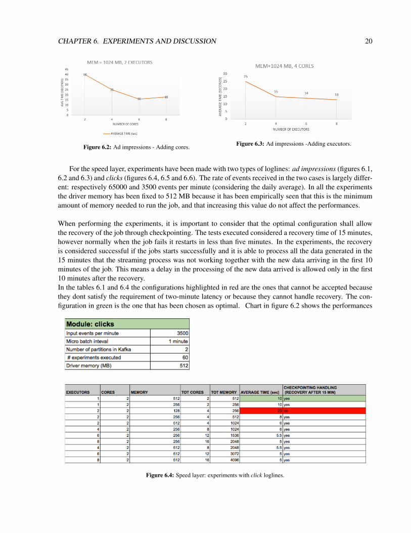
For the speed layer, experiments have been made with two types of loglines: ad impressions (figures 6.1,6.2 and 6.3) and clicks (figures 6.4, 6.5 and 6.6). The rate of events received in the two cases is largely differ-ent: respectively 65000 and 3500 events per minute (considering the daily average). In all the experimentsthe driver memory has been fixed to 512 MB because it has been empirically seen that this is the minimumamount of memory needed to run the job, and that increasing this value do not affect the performances.

When performing the experiments, it is important to consider that the optimal configuration shall allowthe recovery of the job through checkpointing. The tests executed considered a recovery time of 15 minutes,however normally when the job fails it restarts in less than five minutes. In the experiments, the recoveryis considered successful if the jobs starts successfully and it is able to process all the data generated in the15 minutes that the streaming process was not working together with the new data arriving in the first 10minutes of the job. This means a delay in the processing of the new data arrived is allowed only in the first10 minutes after the recovery.In the tables 6.1 and 6.4 the configurations highlighted in red are the ones that cannot be accepted becausethey dont satisfy the requirement of two-minute latency or because they cannot handle recovery. The con-figuration in green is the one that has been chosen as optimal. Chart in figure 6.2 shows the performances

Figure 6.4: Speed layer: experiments with click loglines.


Figure 6.5: Clicks - Adding executors. Figure 6.6: Clicks - Adding memory.

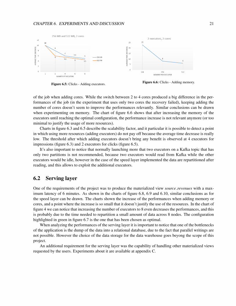
of the job when adding cores. While the switch between 2 to 4 cores produced a big difference in the per-formances of the job (in the experiment that uses only two cores the recovery failed), keeping adding thenumber of cores doesn’t seem to improve the performances relevantly. Similar conclusions can be drawnwhen experimenting on memory. The chart of figure 6.6 shows that after increasing the memory of theexecutors until reaching the optimal configuration, the performance increase is not relevant anymore (or toominimal to justify the usage of more resources).

Charts in figure 6.3 and 6.5 describe the scalability factor, and it particular it is possible to detect a pointin which using more resources (adding executors) do not pay off because the average time decrease is reallylow. The threshold after which adding executors doesn’t bring any benefit is observed at 4 executors forimpressions (figure 6.3) and 2 executors for clicks (figure 6.5).

It’s also important to notice that normally launching more that two executors on a Kafka topic that hasonly two partitions is not recommended, because two executors would read from Kafka while the otherexecutors would be idle, however in the case of the speed layer implemented the data are repartitioned afterreading, and this allows to exploit the additional executors.

6.2 Serving layer

One of the requirements of the project was to produce the materialized view source revenues with a max-imum latency of 6 minutes. As shown in the charts of figure 6.8, 6.9 and 6.10, similar conclusions as forthe speed layer can be drawn. The charts shown the increase of the performances when adding memory orcores, and a point where the increase is so small that it doesn’t justify the use of the resources. In the chart offigure 4 we can notice that increasing the number of executors to 8 even decreases the performances, and thisis probably due to the time needed to repartition a small amount of data across 8 nodes. The configurationhighlighted in green in figure 6.7 is the one that has been chosen as optimal.

When analyzing the performances of the serving layer it is important to notice that one of the bottlenecksof the application is the dump of the data into a relational database, due to the fact that parallel writings arenot possible. However the choice of the data storage for the data warehouse goes beyong the scope of thisproject.

An additional requirement for the serving layer was the capability of handling other materialized viewsrequested by the users. Experiments about it are available at appendix C.


Figure 6.7: Experiments with view source revenues

Figure 6.8: View source revenues - adding cores .Figure 6.9: View source revenues - adding memory .

Figure 6.10: View source revenues - adding executors .

6.3 Experiment results

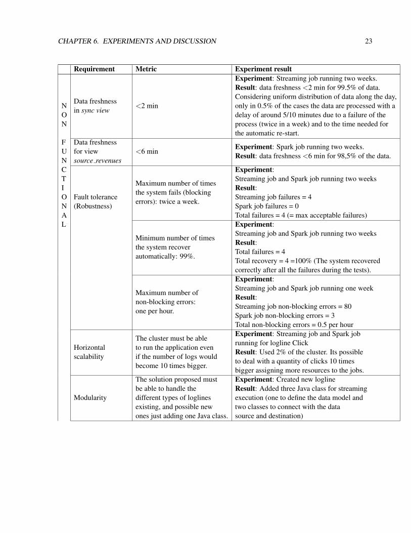
The table 6.1 shows the results of the experiments performed and the satisfaction of the results with respectto the metrics defined for the requirements.


Requirement Metric Experiment result

NON

FUNCTIONAL

Data freshnessin sync view

<2 min

Experiment: Streaming job running two weeks.Result: data freshness <2 min for 99.5% of data.Considering uniform distribution of data along the day,only in 0.5% of the cases the data are processed with adelay of around 5/10 minutes due to a failure of theprocess (twice in a week) and to the time needed forthe automatic re-start.

Data freshnessfor viewsource revenues

<6 minExperiment: Spark job running two weeks.Result: data freshness <6 min for 98,5% of the data.

Fault tolerance(Robustness)

Maximum number of timesthe system fails (blockingerrors): twice a week.

Experiment:Streaming job and Spark job running two weeksResult:Streaming job failures = 4Spark job failures = 0Total failures = 4 (= max acceptable failures)

Minimum number of timesthe system recoverautomatically: 99%.

Experiment:Streaming job and Spark job running two weeksResult:Total failures = 4Total recovery = 4 =100% (The system recoveredcorrectly after all the failures during the tests).

Maximum number ofnon-blocking errors:one per hour.

Experiment:Streaming job and Spark job running one weekResult:Streaming job non-blocking errors = 80Spark job non-blocking errors = 3Total non-blocking errors = 0.5 per hour

Horizontalscalability

The cluster must be ableto run the application evenif the number of logs wouldbecome 10 times bigger.

Experiment: Streaming job and Spark jobrunning for logline ClickResult: Used 2% of the cluster. Its possibleto deal with a quantity of clicks 10 timesbigger assigning more resources to the jobs.

Modularity

The solution proposed mustbe able to handle thedifferent types of loglinesexisting, and possible newones just adding one Java class.

Experiment: Created new loglineResult: Added three Java class for streamingexecution (one to define the data model andtwo classes to connect with the datasource and destination)


Accuracy

There may be duplicateloglines in a maximum spanof 1 minutes andonly for the current day.

Experiment:Streaming job running two weeksResult: The only case in which there may beduplicates is in case that during one micro-batchone executor fails and when it is restartedit re-executes data that had already been insertedin the speed view. This can happen only in therange of data of one micro-batch (1 minute)and the probability that 2 executors fail in thesame day is really low (it never happened duringexperiments). Moreover duplicates may befound only in data of the current day because datafrom the previous ones are always overwritten bythe batch process.

There may be missingloglines in a maximumspan of 1 minutes andonly for the current day.

Experiment:Streaming job running two weeksResult:The only case in which loglines may be missing is ifthey had been processed by a micro-batch but theirpartition has been deleted during the synchronizationphase and data aren’t overwritten by the batch.This can happen only in the range of 1 minute.Example:Micro batch partitions:- Partition1 (18:05:00-18:05:59)- Partition2 (18:06:00-18:06:59)- Partition3 (18:07:00-18:07:59)Batch layer star processing data from 18:06:15, thus itdeletes Partition1 and Partition2. Loglines between the18:06:16 and 18:06:59 will be missing until theexecution of a new batch process.

Loosely Coupled

The solution proposedmust allow to easilychange the destinationstorage (data warehouse)with any of the storagesavailable in the company.

Experiment: Analyzed further storages used in trovit(Apache HDFS, ElasticSearch, Redis)Result:Connectors available that can be easily used tochange the destination storage:- Spark sql for Apache HDFS- Spark-Redis package [14]- Elasticsearch-Hadoop since version 2.1

Interest of the user

The new characteristicsof the process should havea strong positive impact on thedaily work of the data analysts.

75 % of the users said that the project will haveimpact on their job, Among them 25% said that itwill improve their job a lot. Details about thesurvey are in the next section.

Table 6.1: Experiment results


6.3.1 Interest of the user

An online survey has been prepared and submitted to 25 employees in Trovit. The survey was strictlyfocused on the impact of the project on the job of the employees. Thus it was excluding the general impacton Trovit business through the improvement of some of the automatic decision-making processes becausethis cannot be demonstrated before having the project running in production environment for some months.Among the employees targeted, half of them belongs to the sales department and were interviewed aboutthe impact of a smaller data latency in the data warehouse, the other half were business analysts, productmanagers and developers, that were interviewed about the impact of a smaller data latency in the sync view.Both surveys consisted of three questions related to:

• How frequently the employee was accessing the data discussed;• Whether he/she would have accessed them more often in case of a smaller data latency;• The rank of the impact that a smaller data latency would have on their daily work.

The survey was answered by 17 people in total: 8 people within the sales group and 9 people in the secondgroup. In the first group the 75% of the employees said that the project would improve their job, and amongthem the 25% said that the project would improve a lot. The answer of the second group gave similar results(respectively 71% and 28%).The questions used for the survey can be seen in the appendix D.

6.3.2 Comparison with current solution

Tables 6.2 and 6.3 aim to compare the performances of the solution designed and developed with the currentsolution used in the company. This comparison is not aimed to substitute the old solution with the new oneimplemented but it simply wants to analyze the difference of performances of the two technologies used:Hadoop MapReduce and Spark. For this reason when calculating the execution time of the process imple-mented in MapReduce only the phases that are also implemented in Spark have been considered.

The comparison involves the latency and the resources used (memory and cores) in an unit of time.For the new solution, number of cores and memory are calculated summing up the resource used by everyexecutor. For the current solution, implemented with MapReduce, the calculation of the resources usedresulted a bit more complicated because the solution is split in different phases and for each phase thenumber of mappers and reducers change along the day according to the amount of data to process. Thereforethe values displayed in the tables are a weighted average that considers the variation of the number ofmappers and reducers used as well as the time used to execute each phase. When analyzing the resourcesconsumed it is important to notice that both the speed layer and the serving layer implemented in the newsolution are continuous flows that allocate resources the first time they are started and never release them.For the existing solution, instead, resources are allocated when the process is started and released at the end,however the gap between the end of one process and the beginning of the new one is so small than it can beapproximated as the resources would be permanently allocated.

6.3.2.1 Loglines injection

The benchmarking of the current solution and the new implemented solution is shown in table 6.2. Experi-ments were performed using the loglines of type click.


Current solution Speed layer of the new solutionLatency 27 minutes 25 seconds (guaranteed less than 1 minute)Number of cores 4* 4Memory 2400* 1536 (512 for 2 exec + 512 driver)

* approximatively, considering the weighted average of the resources used in the different different phases

Table 6.2: Comparison of the logline injection

6.3.2.2 Serving layer

For the serving layer, experiments were performed using the loglines of type click and the materialized viewsource revenues. The results of the benchmarking are shown in table 6.3. The experiments compare theperformances to dump a materialized view in the data warehouse, and exclude the synchronization phase ofthe new solution.

Current solution Serving layer of the new solutionLatency 3 minutes 85 secondsNumber of cores 7* 8Memory 4000* 1536 (512 for 2 exec + 512 driver)

* approximatively, considering the weighted average of the resources used in the different different phases

Table 6.3: Comparison of the serving layer

Chapter 7

Conclusion and future work

In the last years companies have focused their efforts on near real-time analytics, understanding the impor-tance of reacting on time to possible business changes. The project demonstrated how lambda architecturecan be a good approach for a company to enable near real-time analytics integrating the existing batch pro-cesses with a streaming solution. The experiments showed that all the requirements have been satisfied andthat Apache Spark Streaming resulted to be a good solution for Trovit use case. Moreover some experimentsshowed clearly the better performances of jobs run with Apache Spark and Spark Streaming rather than withHadoop MapReduce, using the same amount of resources (and in some cases even less). This was due tothe fact that in all the use cases the amount of data involved fitted in memory.However during the implementation it became clear how the development of a quite simple ETL flow re-quires lot of work because of the immature technologies. The same ETL would have probably been drawnreally quickly in one of the graphical ETL tools used in traditional Business Intelligence, but currently deal-ing with tools like Spark and with their immaturity is the only way to get good performances. Despite thefact that Apache Spark is a recent technology, it must be acknowledged that the integration with other toolsand databases (Hadoop, Hive, MySql, Kafka) are quite well supported and they resulted an easy step duringthe implementation. Furthermore, analyzing the differences between the new solution implemented (bothspeed layer and serving layer) and the one previously existing (that uses MapReduce and Sqoop), the firstevidence is that the length of the code written in Spark is significantly smaller and more readable. Besidesthese considerations about the technologies involved, however, it is important to remember that the aims ofthe project was not to find an alternative to the data flow implemented in MapReduce but to be able to designand implement a solution that keeping the existing flow would increment the freshness of data to overcomeall the limitations described in section 2.3.The attempt of finding the optimal configuration for each speed layer job running for each type of logline,as well as for each view that has to be executed in the serving layer resulted in a big amount of work. Inthe future a new logic should be created to be able to automatically configure the jobs (number of executors,memory and core assigned, as well as number of partitions) according to the input size of the job. Thiscould be easier for the speed layer where the rate of events arriving is quite stable, more complicated forthe serving layer, where the size of data read should be estimated. Moreover, since the serving layer finaldestination is a relational database, the configuration will also have to take in consideration it, for examplein order not to overload the database with several connections.One of the evident problems of the proposed solution is the maintenance of the code in the batch layer andspeed layer. In fact, even if an effort has been done to share the code between the two layers, still theirimplementation is dependent on their technology (MapReduce for the batch layer and Spark Streaming forthe speed layer) and any future change in the logic should be reflected in both layers.For the two reason just mentioned future research should focus on how to automatically configure the jobs

27

according to their input and to the type of calculations performed but also on how to be able to abstractthe flow implemented so to perform any possible change only once (instead of maintaining the two layersseparately). If this abstraction of the flow, that in this way would be independent from the technology, willbe possible, this will also enable the possibility of choosing the technology according to some parameters.This idea is currently under research and it is based on the awareness that each different technology may bethe best choice in some specific case, according to the input of the job and to the calculations that need tobe performed. In [9] we see an attempt to create a framework that may do exactly this: given a definitionof the input and an high-level data flow definition (not dependent on the implementation), trying to chooseat run time the technology where to run the job, the optimal configuration and to transform the data flow inexecutable code.

28

Appendices

29

Appendix A

Logline

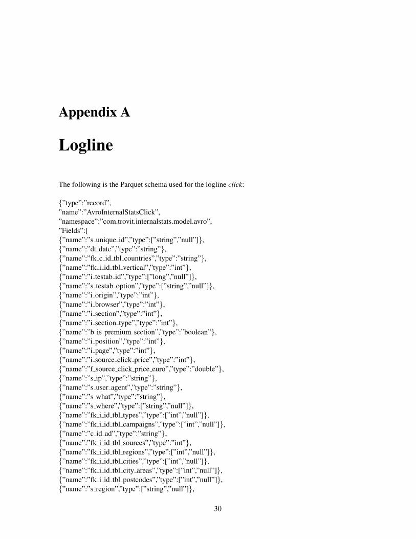
The following is the Parquet schema used for the logline click:

{”type”:”record”,”name”:”AvroInternalStatsClick”,”namespace”:”com.trovit.internalstats.model.avro”,”Fields”:[{”name”:”s unique id”,”type”:[”string”,”null”]},{”name”:”dt date”,”type”:”string”},{”name”:”fk c id tbl countries”,”type”:”string”},{”name”:”fk i id tbl vertical”,”type”:”int”},{”name”:”i testab id”,”type”:[”long”,”null”]},{”name”:”s testab option”,”type”:[”string”,”null”]},{”name”:”i origin”,”type”:”int”},{”name”:”i browser”,”type”:”int”},{”name”:”i section”,”type”:”int”},{”name”:”i section type”,”type”:”int”},{”name”:”b is premium section”,”type”:”boolean”},{”name”:”i position”,”type”:”int”},{”name”:”i page”,”type”:”int”},{”name”:”i source click price”,”type”:”int”},{”name”:”f source click price euro”,”type”:”double”},{”name”:”s ip”,”type”:”string”},{”name”:”s user agent”,”type”:”string”},{”name”:”s what”,”type”:”string”},{”name”:”s where”,”type”:[”string”,”null”]},{”name”:”fk i id tbl types”,”type”:[”int”,”null”]},{”name”:”fk i id tbl campaigns”,”type”:[”int”,”null”]},{”name”:”c id ad”,”type”:”string”},{”name”:”fk i id tbl sources”,”type”:”int”},{”name”:”fk i id tbl regions”,”type”:[”int”,”null”]},{”name”:”fk i id tbl cities”,”type”:[”int”,”null”]},{”name”:”fk i id tbl city areas”,”type”:[”int”,”null”]},{”name”:”fk i id tbl postcodes”,”type”:[”int”,”null”]},{”name”:”s region”,”type”:[”string”,”null”]},

30

{”name”:”s city”,”type”:[”string”,”null”]},{”name”:”s city area”,”type”:[”string”,”null”]},{”name”:”s postcode”,”type”:[”string”,”null”]},{”name”:”i num pictures”,”type”:[”int”,”null”]},{”name”:”b nrt”,”type”:”boolean”},{”name”:”b is publish your ad”,”type”:[”boolean”,”null”]},{”name”:”b out of budget”,”type”:[”boolean”,”null”]},{”name”:”i suggester”,”type”:[”int”,”null”]},{”name”:”s agency”,”type”:[”string”,”null”]},{”name”:”s make”,”type”:[”string”,”null”]},{”name”:”fk i id tbl makes”,”type”:[”int”,”null”]},{”name”:”s model”,”type”:[”string”,”null”]},{”name”:”fk i id tbl models”,”type”:[”int”,”null”]},{”name”:”s car dealer”,”type”:[”string”,”null”]},{”name”:”s company”,”type”:[”string”,”null”]},{”name”:”fk i id tbl companies”,”type”:[”int”,”null”]},{”name”:”s category”,”type”:[”string”,”null”]},{”name”:”fk i id tbl categories”,”type”:[”int”,”null”]},{”name”:”b is new”,”type”:[”boolean”,”null”]},{”name”:”s v”,”type”:[”string”,”null”]},{”name”:”s pageview id”,”type”:[”string”,”null”]},{”name”:”fk i id tbl dealer type”,”type”:[”int”,”null”]},{”name”:”fk i id tbl pricing type”,”type”:[”int”,”null”]},{”name”:”s cookie id”,”type”:[”string”,”null”]},{”name”:”s google id”,”type”:[”string”,”null”]},{”name”:”fk i id tbl users”,”type”:[”int”,”null”]},{”name”:”b valid”,”type”:[”boolean”,”null”]},{”name”:”b out of budget original”,”type”:[”boolean”,”null”]},{”name”:”i campaign type”,”type”:[”int”,”null”]},{”name”:”i click type”,”type”:[”int”,”null”]} ]}

31

Appendix B

Agile Methodology

The work of the Master Thesis was held with the collaboration of a team of five people working in Trovit.For the realization of the project the Agile development methodology has been followed. In particular, thefollowing actions have been taken:

• daily meetings (around 10 minutes) where each team member explains what has been done and whatis planned to do during the day;• weekly sprints where each team member explains the tasks that he has completed and new tasks are

assigned;• quarterly retrospective meeting to discuss how the team is doing and the points to improve.

The project of the Master Thesis has been initially divided into macro-tasks and then split into smallest tasksthat have been added to the already existing product backlog of the team. Figure B.1 shows the schedule ofthe sprints in which the project was involved. Table B.2 is an excerpt of the team product backlog containingonly the tasks related to the Master Thesis project.

32

Figure B.1: Weekly sprints.

33

Figure B.2: Product backlog.

34

Appendix C

Additional views for the data warehouse

An additional requirement for the serving layer was the capability of handling other materialized viewsrequested by the users. Experiments have been made to find an optimal configuration for two additionalmaterialized views. With respect to the source revenues view previously analyzed, these views have to dealwith a larger amount of data, for this reason they will have different requirements. The requirements thathave been set are:

• The two views must run in the same application (thus finding a common configuration).• Maximum data freshness for view hit zone montlhy = 12 minutes.• Maximum data freshness for view source revenues hourly = 7 minutes.

Highlighted in green in figures C.1 and C.2 is the configuration that can satisfy all the requirements for thetwo views.

Figure C.1: Experiments view hit zone monthly

35

Figure C.2: Experiments view source revenues hourly

36

Appendix D

Survey

D.1 First survey

The first survey targeted employees from the sales department. The questions are related to the viewtbl source revenues of the data warehouse, as well as to some screenshots shown to the employees aboutstatistics that are available on Trovit internal website.

1. How many times a week do you look at one of the tables above (screenshots from Bate) or do youquery the table tbl source revenues on MySql?- Never- Once a week- Every day- More than once a day

2. Currently these tables are updated every hour and a half. Do you think that you would look at themmore often if they would be updated every 6 minutes?- Yes- No- I don’t know

3. If they would be updated every 6 minutes, from 1 to 5 how much do you think this would impactin your work? (where 1 means ”this would not improve my work” and 5 means ”my work wouldimprove a lot”)

D.2 Second survey

The second survey targeted business analysts, product managers and developers and it was related to thetable tbl internalstats clicks, that is the table of the sync view containing the loglines of type clicks. Thequestions were the following:

1. How many times a week do you query the table tbl internalstats clicks using Hive or Impala?- Never- Once a week- Every day- More than once a day

37

2. Currently this table is updated every hour. Do you think that you would look at it more often if itwould be updated every 2 minutes?- Yes- No- I don’t know

3. If it would be updated every 2 minutes, from 1 to 5 how much do you think this would impact yourwork? (where 1 means ”this would not improve my work” and 5 means ”my work would improve alot”)

38

References

[1] Nathan Marz with James Warren. “Big Data: Principles and best practices of scalable realtime datasystems”. In: Manning Publications, 2015. Chap. 1.7.

[2] Trovit website. URL: http://www.trovit.es.

[3] How to choose a data format. URL: http://www.svds.com/how-to-choose-a-data-format.

[4] Data formats. URL: http://www.svds.com/dataformats/.

[5] Nathan Marz with James Warren. “Big Data: Principles and best practices of scalable realtime datasystems”. In: Manning Publications, 2015. Chap. 1.6.

[6] Kappa architecture. URL: http://milinda.pathirage.org/kappa-architecture.com/.

[7] Zeta architecture. URL: https://www.mapr.com/solutions/zeta-enterprise-architecture.

[8] Lambda architecture repository. URL: http://lambda-architecture.net/.

[9] Natacha Crooks Matthew P. Grosvenor Allen Clement Steven Hand Ionel Gog Malte Schwarzkopf.“Musketeer: all for one, one for all in data processing systems”. In: (2015).

[10] Apache Showdown: Flink vs Spark. URL: https://tech.zalando.de/blog/apacheshowdown-flink-vs.-spark/.

[11] Spark documentation: transformations on DStreams. URL: http://spark.apache.org/docs/latest/streaming-programming-guide.html#transformations-on-dstreams.

[12] Sentry. URL: https://getsentry.com/welcome/.

[13] Graphite. URL: http://graphiteapp.org/.

[14] Spark-Redis connector. URL: https://spark-packages.org/package/RedisLabs/spark-redis.

39

Implementing the speed layer in a lambda architecture -...

Documents

Transcript of Implementing the speed layer in a lambda architecture -...