Kristine Jolivette, Ph.D. Jeffrey Sprague, Ph.D. Brenda Scheuermann, Ph.D.

Md. Nafiul Haque (Ph.D. Candidate)
Murad Y. Abu-Farsakh, Ph.D., P.E.
Louisiana Transportation Conference March 1, 2016
Implementation of Pile Setup in
the LRFD Design of Driven Piles
in Louisiana
OUTLINE
Objectives
Brief Background
Methodology
Results and Analysis
Analytical Models
LRFD Calibration
2
OBJECTIVES
Evaluate the time-dependant increase in pile capacity
(or setup) for piles driven into Louisiana soils through
conducting repeated static and dynamic field testing
with time on full-scale instrumented test piles.
Study the effect of soil type/properties, pile size, and
their interaction on pile setup phenomenon.
Develop analytical model(s) to estimate pile setup with
time using typical soil properties.
Incorporate setup into LRFD design of driven pile in
Louisiana (calibrate setup resistance factor, fsetup).
3
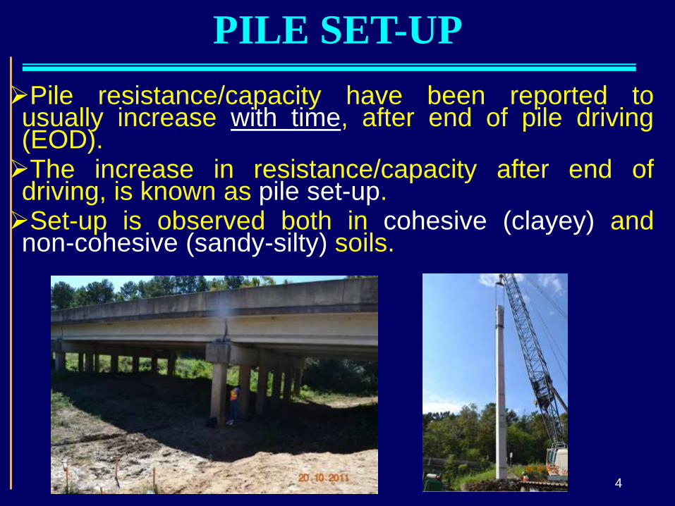
PILE SET-UP
Pile resistance/capacity have been reported to usually increase with time, after end of pile driving (EOD). The increase in resistance/capacity after end of driving, is known as pile set-up. Set-up is observed both in cohesive (clayey) and non-cohesive (sandy-silty) soils.
4

Benefits of Incorporating Set-up in Design
The implementation of pile set-up capacity in the design can result in significant cost savings through
Shortening pile lengths
Reducing pile cross-sectional area (using smaller-diameter/width piles)
Smaller hammer to drive pile
Reducing the number of piles Substantial cost will be saved for full project
5
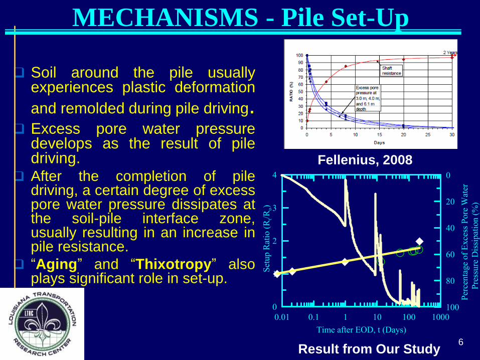
MECHANISMS - Pile Set-Up
Soil around the pile usually experiences plastic deformation
and remolded during pile driving. Excess pore water pressure
develops as the result of pile driving.
After the completion of pile driving, a certain degree of excess pore water pressure dissipates at the soil-pile interface zone, usually resulting in an increase in pile resistance.
“Aging” and “Thixotropy” also plays significant role in set-up.
Fellenius, 2008
Result from Our Study 6

MECHANISMS - Pile Set-Up In cohesive soils, the induced excess pore water pressure may dissipate
slowly due to low permeability and it takes 50-100 days to dissipate.
However, for noncohesive soils, the duration of dissipation of excess pore
water pressure take several hours to several days due to high
permeability.
This dissipation phase plays the most significant role for the set-up
phase / period or how long it will take for the completion of set-up.
Sandy Soil Clayey Soil
7
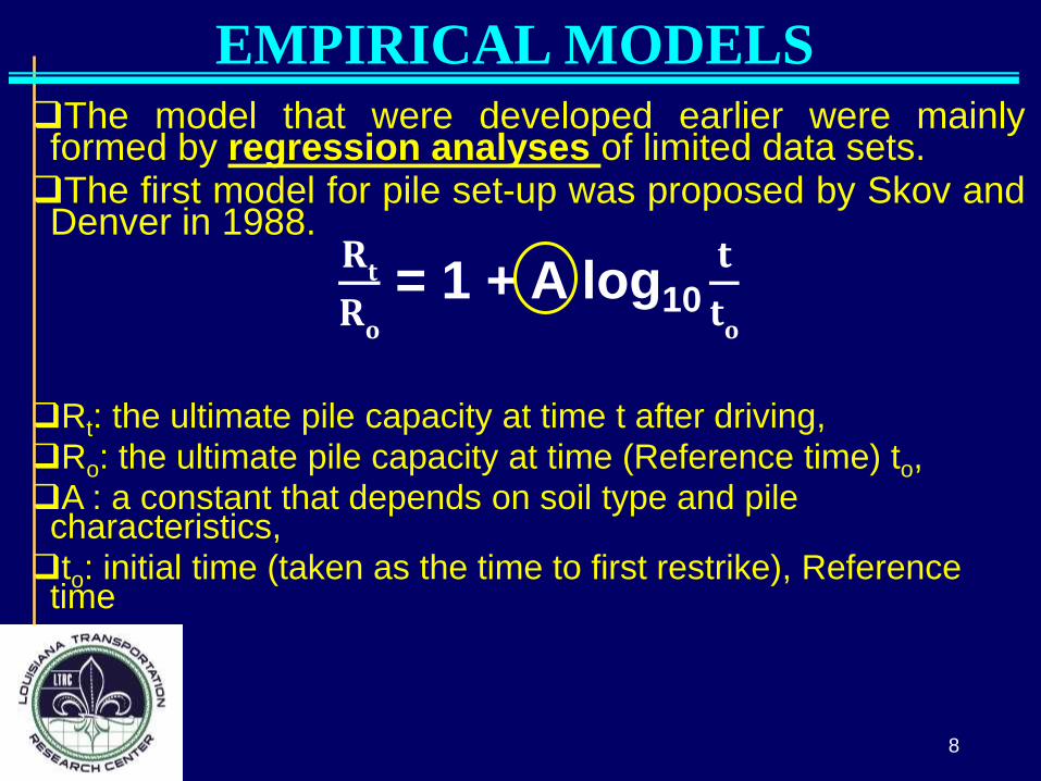
EMPIRICAL MODELS
The model that were developed earlier were mainly formed by regression analyses of limited data sets. The first model for pile set-up was proposed by Skov and Denver in 1988.
𝐑
𝐭
𝐑𝐨
= 1 + A log10 𝐭
𝐭𝐨
Rt: the ultimate pile capacity at time t after driving,
Ro: the ultimate pile capacity at time (Reference time) to, A : a constant that depends on soil type and pile
characteristics,
to: initial time (taken as the time to first restrike), Reference time
8
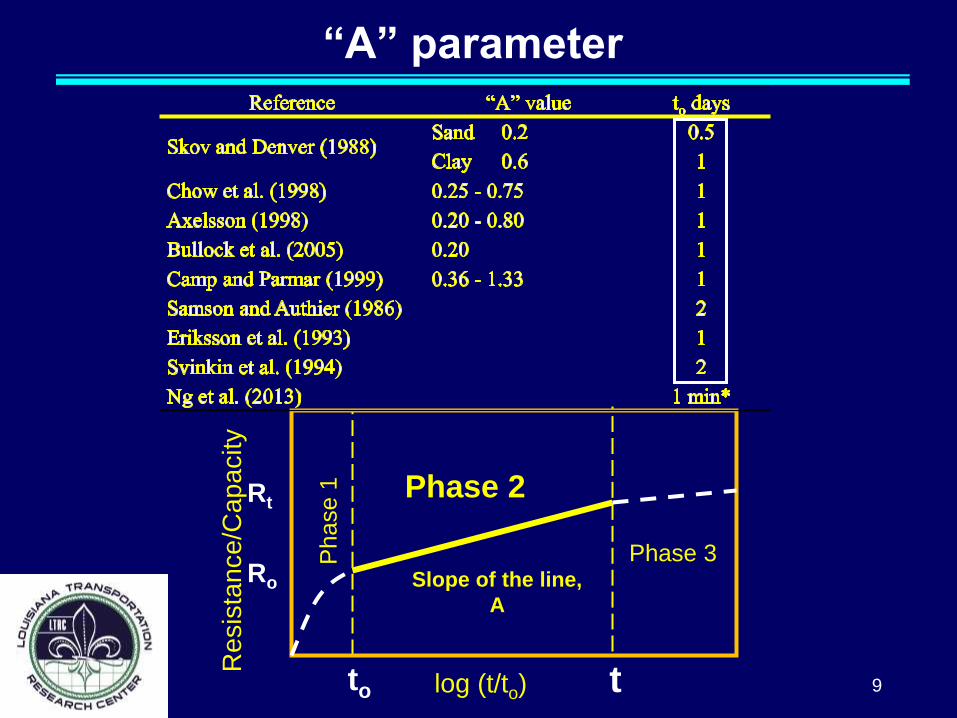
“A” parameter
9 log (t/to)
Phase 2
Phase 3 Phase 1
Re
sis
tan
ce
/Cap
acity
to t
Ro
Rt
Slope of the line,
A
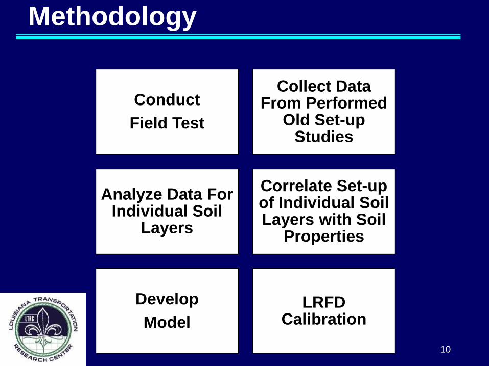
Methodology
10
Conduct
Field Test
Collect Data From Performed
Old Set-up Studies
Analyze Data For Individual Soil
Layers
Correlate Set-up of Individual Soil Layers with Soil
Properties
Develop
Model
LRFD Calibration
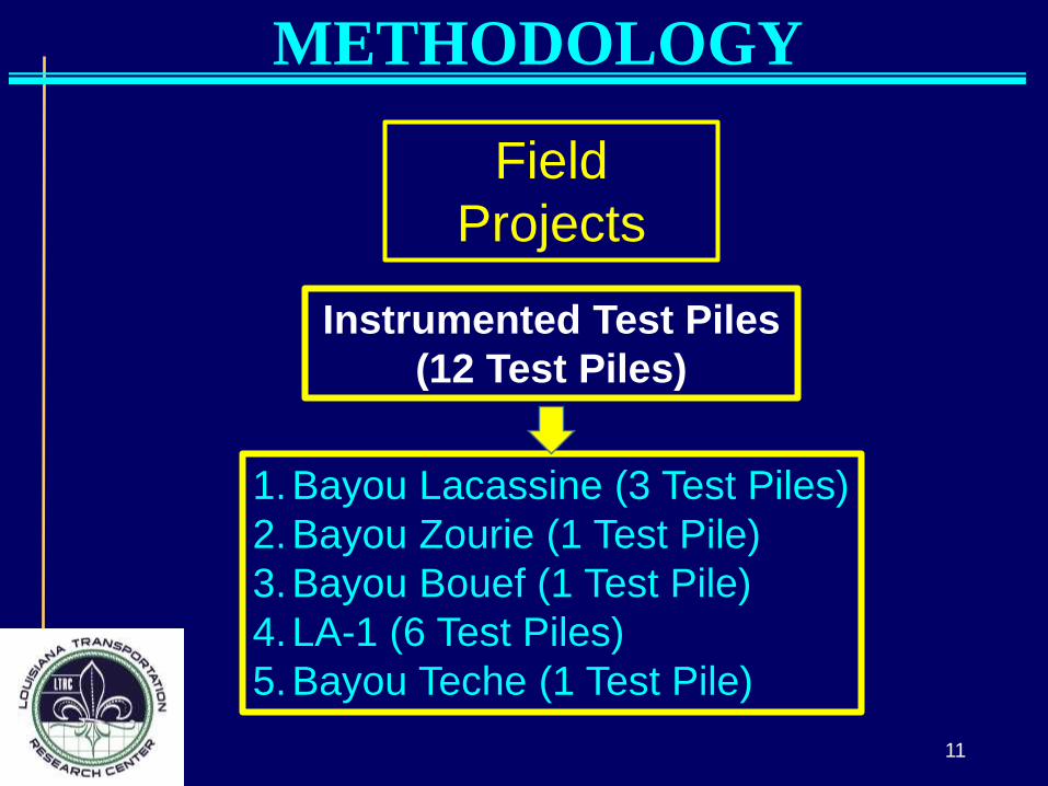
Field
Projects
Instrumented Test Piles
(12 Test Piles)
METHODOLOGY
11
1.Bayou Lacassine (3 Test Piles)
2.Bayou Zourie (1 Test Pile)
3.Bayou Bouef (1 Test Pile)
4.LA-1 (6 Test Piles)
5.Bayou Teche (1 Test Pile)

12
METHODOLOGY-FIELD PROJECTS
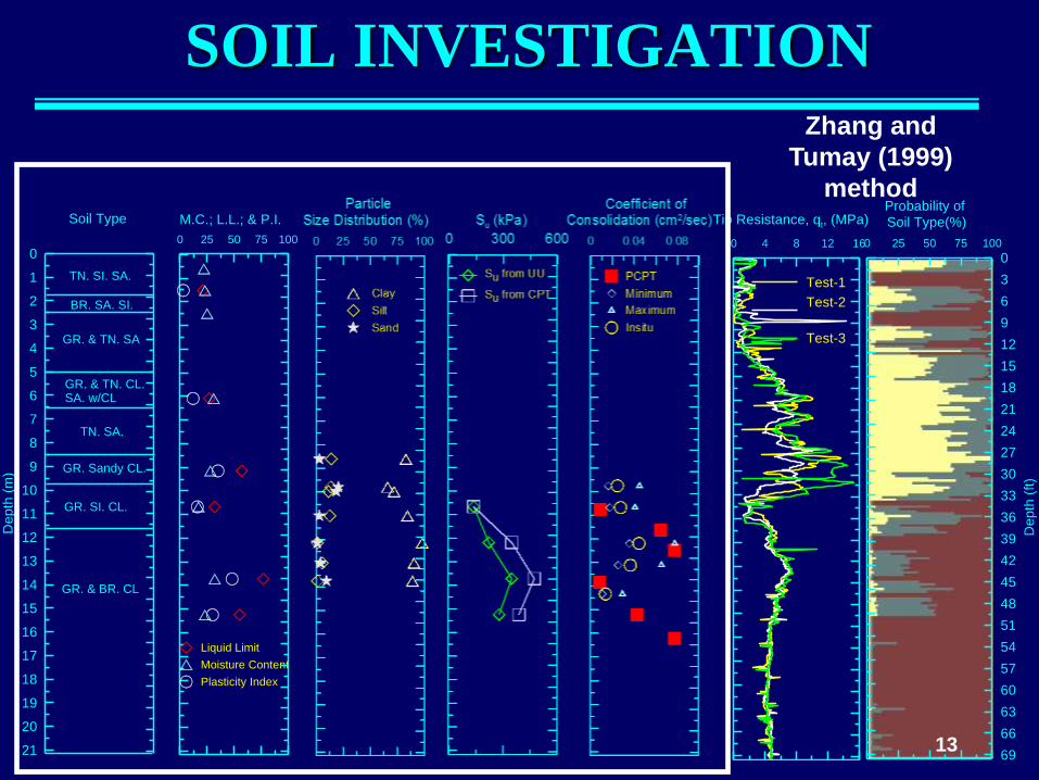
SOIL INVESTIGATION
Test-1
Test-2
Test-3
0 4 8 12 16
Tip Resistance, qt, (MPa)
0
3
6
9
12
15
18
21
24
27
30
33
36
39
42
45
48
51
54
57
60
63
66
69
De
pth
(ft)
0 25 50 75 100
Probability of
Soil Type(%)
TN. SI. SA.
21
20
19
18
17
16
15
14
13
12
11
10
9
8
7
6
5
4
3
2
1
0
De
pth
(m
)
Soil Type
GR. & TN. SA
GR. & TN. CL.SA. w/CL
BR. SA. SI.
Liquid Limit
Moisture Content
Plasticity Index
0 25 50 75 100
M.C.; L.L.; & P.I.
Clay
Silt
Sand
0 25 50 75 100
Particle
Size Distribution (%)
Su from UU
Su from CPT
0 300 600
Su (kPa)
TN. SA.
GR. & BR. CL
GR. SI. CL.
PCPT
Minimum
Maximum
Insitu
0 0.04 0.08
Coefficient of
Consolidation (cm2/sec)
GR. Sandy CL.
13
Zhang and
Tumay (1999)
method

Dissipation Tests to Calculate cv
1 10 100 1000 10000Time (sec)
0
0.3
0.6
0.9
1.2
1.5
No
rmali
zed
Ex
ces
s P
ore
W
ate
r P
ress
ure
( u
/ui)
12.36 m
17.38 m
14.35 m
15.231 m
16.332 m
9.19 m
11.35 m
BL-TP-1
1 10 100 1000 10000Time (sec)
0
0.3
0.6
0.9
1.2
1.5
No
rmali
zed
Ex
ces
s P
ore
W
ate
r P
ress
ure
( u
/ui)
13.34 m
11.93 m8.38 m
18.34 m
5.14 m
6.38 m
14.42 m10.39 m
BL-TP-3
Bayou
Zourrie
14

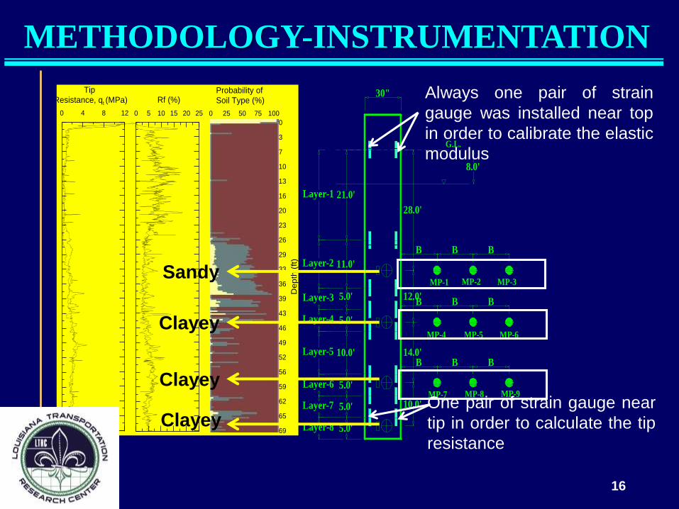
METHODOLOGY-INSTRUMENTATION
Sister bar Strain gauges Pressure cells Piezometers Multilevel Piezometers
Soil Profile 15
Sandy
Clayey
Clayey
Clayey
Sandy
Sandy
Cv from Lab
Cv from PCPT
1E-005 0.001 0.1
Coefficient of
Consolidation (cm2/sec)
0 25 50 75 100
M.C.; L.L; & P.I.
.Su from UU
Su from CPT
0 100 200 300
Su (kPa)
Liquid Limit
Plasticity Index
Moisture Content
BR & Light Gr., Organic Clay, OH
Light Br.,Silty Clay, CL
21
20
19
18
17
16
15
14
13
12
11
10
9
8
7
6
5
4
3
2
1
0
De
pth
(m
)
Soil Type
Light Gr.,Organic Clay, OH
Gr., Silty Clay CL
Dark Gr.,Silty Clay, CL
Gr., Lean Clay CL
Reddish Light Br.,SIlty Clay, CL
Light Br.,Sandy Clay, CH
Light Br., Silty Clay, CL
Dark Gr.,Sandy Clay, CL
OCR from CPT
OCR from Lab
0 1 2 3 4 5
OCR
0 4 8 12
Tip
Resistance, qt (MPa)
0 5 10 15 20 25
Rf (%)
69
65
62
59
56
52
49
46
43
39
36
33
29
26
23
20
16
13
10
7
3
0
De
pth
(ft
)
0 25 50 75 100
Probability of
Soil Type (%)
Casing
30"
21.0'
11.0'
5.0'
5.0'
10.0'
5.0'
28.0'
12.0'
14.0'
10.0'
5.0'
5.0'
B B B
B
B
B
B
B
B
G.L.
8.0'
MP-7 MP-8 MP-9
MP-4 MP-5 MP-6
MP-1 MP-2 MP-3
Layer-8
Layer-7
Layer-6
Layer-5
Layer-4
Layer-3
Layer-2
Layer-1
Sandy
Clayey
Clayey
Clayey
Always one pair of strain
gauge was installed near top
in order to calibrate the elastic
modulus
One pair of strain gauge near
tip in order to calculate the tip
resistance
16
METHODOLOGY-INSTRUMENTATION
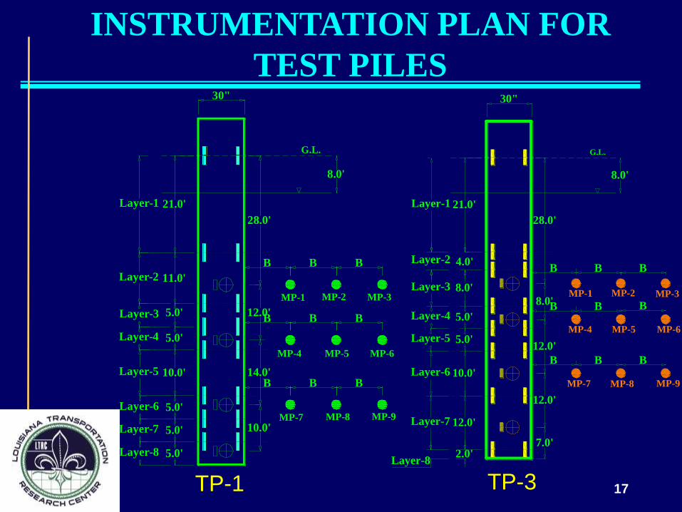
INSTRUMENTATION PLAN FOR
TEST PILES 30"
21.0'
11.0'
5.0'
5.0'
10.0'
5.0'
28.0'
12.0'
14.0'
10.0'
5.0'
5.0'
B B B
B
B
B
B
B
B
G.L.
8.0'
MP-7 MP-8 MP-9
MP-4 MP-5 MP-6
MP-1 MP-2 MP-3
Layer-8
Layer-7
Layer-6
Layer-5
Layer-4
Layer-3
Layer-2
Layer-1
TP-1
30"
21.0'
4.0'
8.0'
5.0'
5.0'
10.0'
12.0'
7.0'
8.0'
12.0'
12.0'
28.0'
8.0'
G.L.
B B B
B
B
B
B
B
B
MP-7 MP-8 MP-9
MP-4 MP-5 MP-6
MP-1 MP-2 MP-3
Layer-7
Layer-6
Layer-5
Layer-4
Layer-3
Layer-2
Layer-1
Layer-82.0'
TP-3 17
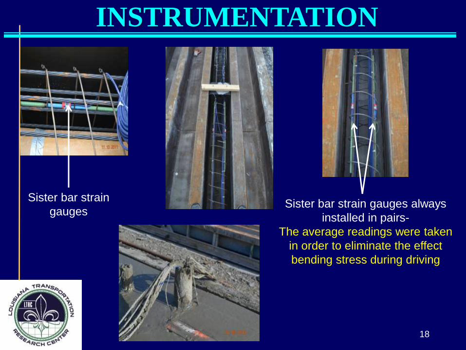
Sister bar strain
gauges Sister bar strain gauges always
installed in pairs-
The average readings were taken
in order to eliminate the effect
bending stress during driving
18
INSTRUMENTATION

Pressure cell
Piezometer
Pressure cell & Piezometer
Geokon Model 4820
Geokon Model 4500S
19
INSTRUMENTATION

Before
Pouring
Concrete
After
Pouring
Concrete
Installed in
predefined
depth
20
INSTRUMENTATION
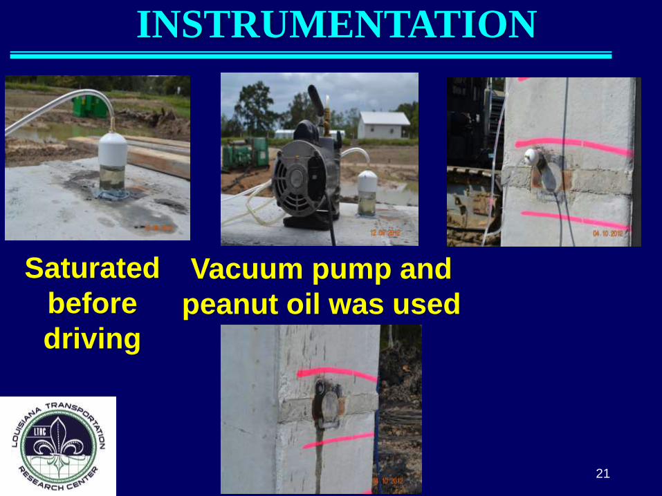
Saturated
before
driving
Vacuum pump and
peanut oil was used
21
INSTRUMENTATION
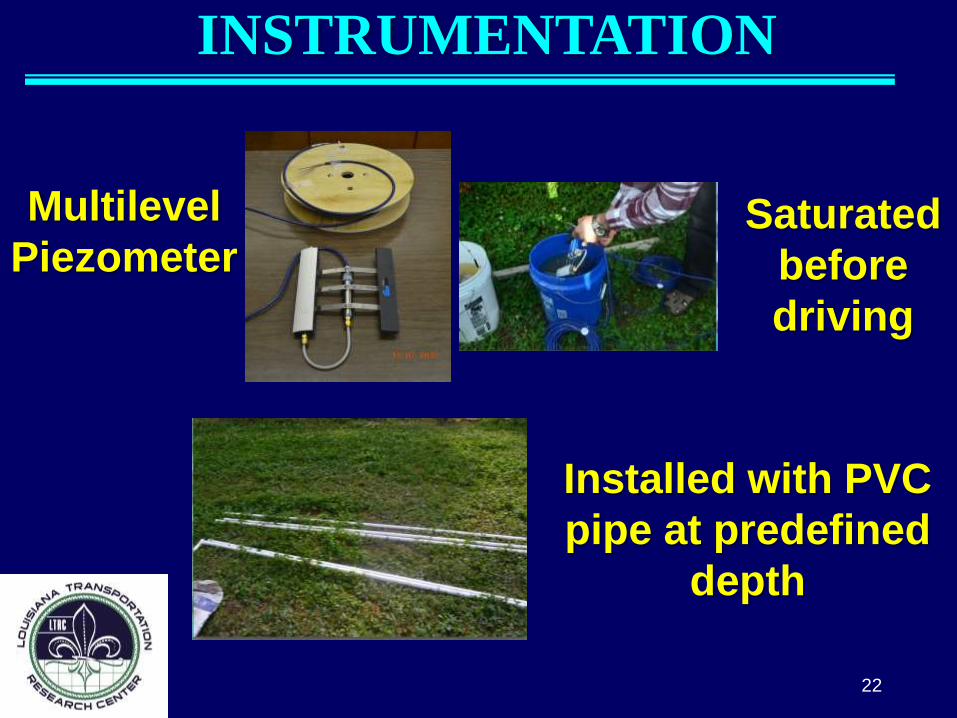
Saturated
before
driving
Multilevel
Piezometer
Installed with PVC
pipe at predefined
depth
22
INSTRUMENTATION

INSTRUMENTATION
A data collection
system composed
of CR-1000,
multiplexels and
solar panel was
there for six
months
All the wires were
pulled out through
a PVC pipe near
the top of pile
The wires were
connected to a
data logger
system through a
trench
23

DRIVING AND LOAD TESTS
Hammer
Accelerometer
and strain
transducer PDA
device
24

STATIC LOAD TESTS
25

BAYOU LACASSINE
26
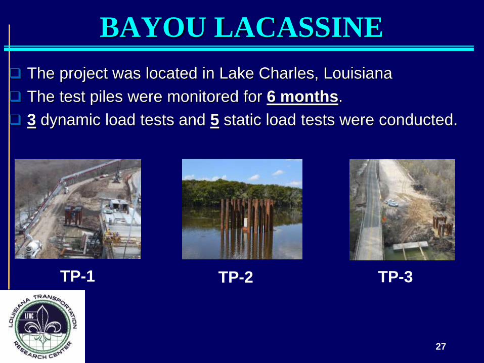
The project was located in Lake Charles, Louisiana
The test piles were monitored for 6 months.
3 dynamic load tests and 5 static load tests were conducted.
TP-2 TP-1 TP-3
27
BAYOU LACASSINE
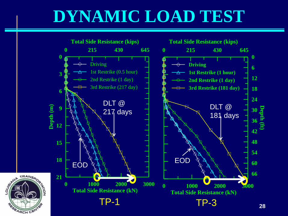
DYNAMIC LOAD TEST
0 1000 2000 3000Total Side Resistance (kN)
0 215 430 645
Total Side Resistance (kips)
66
60
54
48
42
36
30
24
18
12
6
0
Dep
th (ft)
.Driving
1st Restrike (1 hour)
2nd Restrike (1 day)
3rd Restrike (181 day)
TP-3
EOD
DLT @
181 days
EOD
0 1000 2000 3000Total Side Resistance (kN)
21
18
15
12
9
6
3
0D
epth
(m
)0 215 430 645
Total Side Resistance (kips)
.Driving
1st Restrike (0.5 hour)
2nd Restrike (1 day)
3rd Restrike (217 day)
TP-1
DLT @
217 days
28
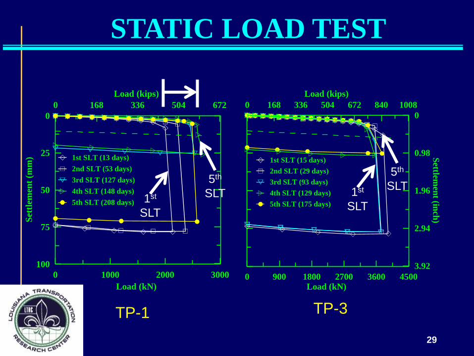
STATIC LOAD TEST
29
0 1000 2000 3000
Load (kN)
100
75
50
25
0
Set
tlem
ent
(mm
)
0 168 336 504 672
Load (kips)
.1st SLT (13 days)
2nd SLT (53 days)
3rd SLT (127 days)
4th SLT (148 days)
5th SLT (208 days)
TP-1
0 900 1800 2700 3600 4500Load (kN)
0 168 336 504 672 840 1008
Load (kips)
3.92
2.94
1.96
0.98
0
Settlem
ent (in
ch)
.1st SLT (15 days)
2nd SLT (29 days)
3rd SLT (93 days)
4th SLT (129 days)
5th SLT (175 days)
TP-3
1st
SLT
5th
SLT 1st
SLT
5th
SLT
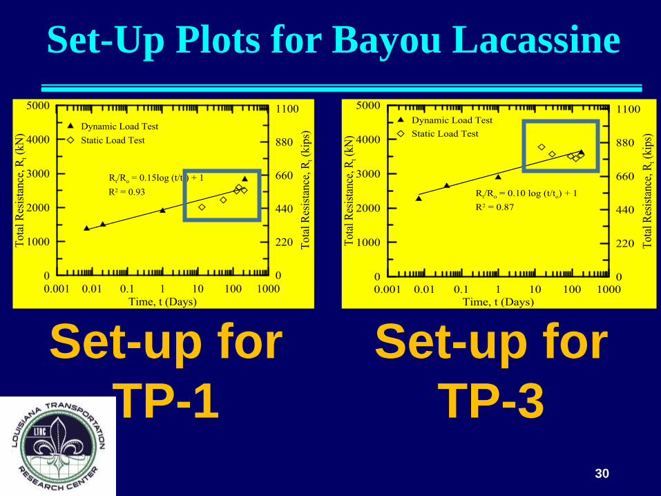
Set-Up Plots for Bayou Lacassine
Set-up for
TP-1
Set-up for
TP-3
30
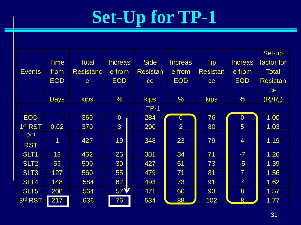
Set-Up for TP-1
Events
Time
from
EOD
Total
Resistanc
e
Increas
e from
EOD
Side
Resistan
ce
Increas
e from
EOD
Tip
Resistan
ce
Increas
e from
EOD
Set-up
factor for
Total
Resistan
ce
Days kips % kips % kips % (Rt/Ro)
TP-1
EOD - 360 0 284 0 76 0 1.00
1st RST 0.02 370 3 290 2 80 5 1.03
2nd
RST 1 427 19 348 23 79 4 1.19
SLT1 13 452 26 381 34 71 -7 1.26
SLT2 53 500 39 427 51 73 -5 1.39
SLT3 127 560 55 479 71 81 7 1.56
SLT4 148 584 62 493 73 91 7 1.62
SLT5 208 564 57 471 66 93 8 1.57
3rd RST 217 636 76 534 88 102 8 1.77
31
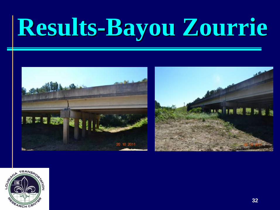
Results-Bayou Zourrie
32

Events Time Side
Resistance
Tip
Resistance Total Resistance
kips % kips % kips %
Driven 0 365 - 237 - 2678/602 -
1st Dynamic Load Test 1 hr 457 25 221 -7 3016/678 13
2nd Dynamic Load Test 1 day 471 29 245 3 3185/716 19
1st Static Load Test 14 days
2nd Static Load Test 30 days
3rd Dynamic Load Test 78 days 656 80 222 -6 3906/878 46
0.01 0.1 1 10 100
Time, t (Days)
0
1000
2000
3000
4000
5000
6000
Pil
e R
esis
tan
ce, Q
R (
kN
)
0
225
450
674
899
1124
1349
Pil
e R
esis
tan
ce,Q
R (
kip
s)
R2 = 0.93
Set-up Results for Bayou Zourrie
33

LA-1
TP-2 TP-3
TP-4 TP-5 34
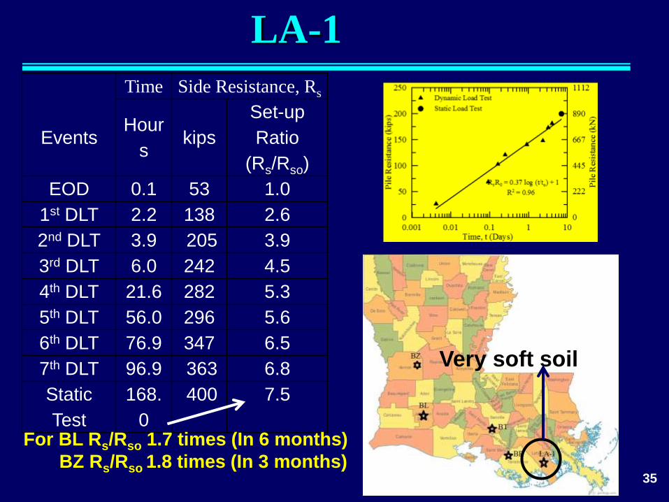
Events
Time Side Resistance, Rs
Hour
s kips
Set-up
Ratio
(Rs/Rso)
EOD 0.1 53 1.0
1st DLT 2.2 138 2.6
2nd DLT 3.9 205 3.9
3rd DLT 6.0 242 4.5
4th DLT 21.6 282 5.3
5th DLT 56.0 296 5.6
6th DLT 76.9 347 6.5
7th DLT 96.9 363 6.8
Static
Test
168.
0
400 7.5
For BL Rs/Rso 1.7 times (In 6 months)
BZ Rs/Rso 1.8 times (In 3 months)
Very soft soil
35
LA-1

Set-Up for
Bayou Teche and Bayou Bouef
Rs/Rso 1.9 times
(In 32 days)
Bayou Teche Bayou Bouef
Rs/Rso 3.8 times
(In 716 days-almost 2 years)
36

Pile Set-Up (Result of 12 Test Piles)
The result is consistent with literature that
set-up fits best with linear logarithmic of time
37

Set-Up Process with
Consolidation Behavior
0.001 0.01 0.1 1 10 100 1000
Time after EOD, t (Days)
100
80
60
40
20
0
Per
cen
tage
of
Exce
ss P
ore
Wa
ter
P
ress
ure
Dis
sip
ati
on
(%
)
8.54 m deep
12.20 m deep
16.47 m deep
19.52 m deep
2nd Restrike1st SLT
3rd SLT 4th SLT
5th SLT
Installation of Load Frame
2nd SLT
TP-1
0.001 0.01 0.1 1 10 100 1000
Time after EOD, t (Days)
100
80
60
40
20
0
8.54 m deep
10.98 m deep
14.64 m deep
18.30 m deep
2nd Restrike
1st SLT
3rd SLT
4th SLT
5th SLT
Installation of Load Frame
2nd SLT
TP-3
Set-up continues for
127 days No set-up after 15
days 38

Set-Up Process with
Consolidation Behavior By Layers
Smaller amount of set-up or low
rate of set-up as consolidation
process finished earlier
Higher amount or rate of set-up as
consolidation process continued for
longer period of time
39

Set-Up for Individual Soil Layers
Load Distribution Plot
Load-Strain Plot
Modulus-Strain Plot
P = E x ξ x A
Tip
Resistance
Used to calculate the
resistance of individual soil
layers
40
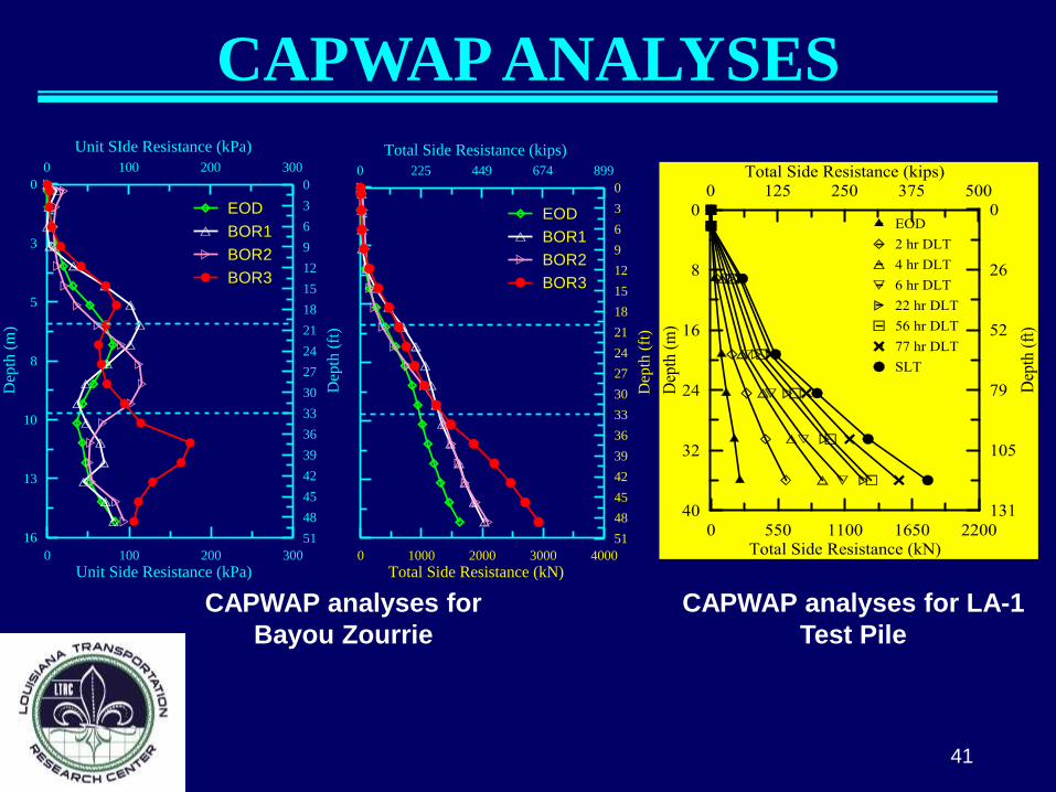
CAPWAP ANALYSES
CAPWAP analyses for
Bayou Zourrie
CAPWAP analyses for LA-1
Test Pile
0 100 200 300
Unit Side Resistance (kPa)
16
13
10
8
5
3
0
Dep
th (
m)
0 100 200 300
Unit SIde Resistance (kPa)
51
48
45
42
39
36
33
30
27
24
21
18
15
12
9
6
3
0
Dep
th (
ft)
EOD
BOR1
BOR2
BOR3
0 1000 2000 3000 4000
Total Side Resistance (kN)
16
13
10
8
5
3
0
Dep
th (
m)
0 225 449 674 899
Total Side Resistance (kips)
51
48
45
42
39
36
33
30
27
24
21
18
15
12
9
6
3
0
Dep
th (
ft)
.
EOD
BOR1
BOR2
BOR3
41
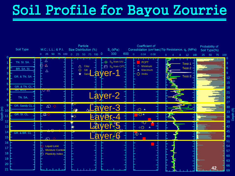
Soil Profile for Bayou Zourrie
Test-1
Test-2
Test-3
0 4 8 12 16
Tip Resistance, qt, (MPa)
0
3
6
9
12
15
18
21
24
27
30
33
36
39
42
45
48
51
54
57
60
63
66
69
De
pth
(ft)
0 25 50 75 100
Probability of
Soil Type(%)
Layer-1
TN. SI. SA.
21
20
19
18
17
16
15
14
13
12
11
10
9
8
7
6
5
4
3
2
1
0
De
pth
(m
)
Soil Type
GR. & TN. SA
GR. & TN. CL.SA. w/CL
BR. SA. SI.
Liquid Limit
Moisture Content
Plasticity Index
0 25 50 75 100
M.C.; L.L.; & P.I.
Clay
Silt
Sand
0 25 50 75 100
Particle
Size Distribution (%)
Su from UU
Su from CPT
0 300 600
Su (kPa)
TN. SA.
GR. & BR. CL
GR. SI. CL.
PCPT
Minimum
Maximum
Insitu
0 0.04 0.08
Coefficient of
Consolidation (cm2/sec)
GR. Sandy CL.
Layer-2
Layer-3 Layer-4 Layer-5 Layer-6
42
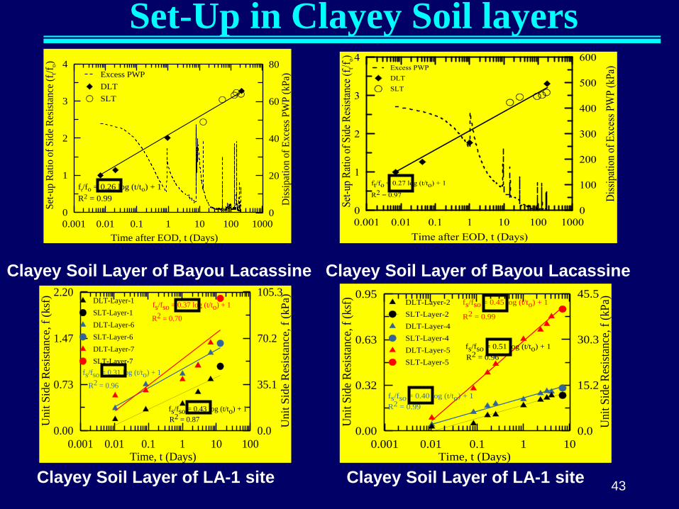
Set-Up in Clayey Soil layers
0.001 0.01 0.1 1 10 100 1000
Time after EOD, t (Days)
0
1
2
3
4
Set
-up R
atio
of
Sid
e R
esis
tance
(f t/f
o)
0
20
40
60
80
Dis
sipat
ion o
f E
xce
ss P
WP
(kP
a)
Excess PWP
DLT
SLT
ft/fo = 0.26 log (t/to) + 1
R2 = 0.99
Clayey Soil Layer of Bayou Lacassine Clayey Soil Layer of Bayou Lacassine
0.001 0.01 0.1 1 10 100Time, t (Days)
0.00
0.73
1.47
2.20
Unit
Sid
e R
esis
tance,
f (
ksf
)
0.0
35.1
70.2
105.3U
nit
Sid
e R
esis
tance
, f
(kP
a)DLT-Layer-1
SLT-Layer-1
DLT-Layer-6
SLT-Layer-6
DLT-Layer-7
SLT-Layer-7
R2 = 0.96
fs/fso = 0.31 log (t/to) + 1
fs/fso = 0.37 log (t/to) + 1
R2 = 0.70
fs/fso = 0.43 log (t/to) + 1
R2 = 0.87
Clayey Soil Layer of LA-1 site
0.001 0.01 0.1 1 10Time, t (Days)
0.00
0.32
0.63
0.95
Unit
Sid
e R
esis
tance
, f
(ksf
)
0.0
15.2
30.3
45.5
Unit
Sid
e R
esis
tance
, f
(kP
a)DLT-Layer-2
SLT-Layer-2
DLT-Layer-4
SLT-Layer-4
DLT-Layer-5
SLT-Layer-5
R2 = 0.99
fs/fso = 0.40 log (t/to) + 1
fs/fso = 0.45 log (t/to) + 1
R2 = 0.99
fs/fso = 0.51 log (t/to) + 1
R2 = 0.96
Clayey Soil Layer of LA-1 site 43

Set-Up in Sandy Soil layers
Sandy Soil Layer of Bayou Zourie Sandy Soil Layer of Bayou Lacassine
0.001 0.01 0.1 1 10 100Time, t (Days)
0.00
0.93
1.87
2.80
Unit
Sid
e R
esis
tance
, f
(ksf
)
0.0
44.7
89.4
134.1U
nit
Sid
e R
esis
tance
, f
(kP
a)DLT-Layer-2
SLT-Layer-2
SLT-Layer-5
SLT-Layer-5
DLT-Layer-8
R2 = 0.94
fs/fso = 0.08 log (t/to) + 1
fs/fso = 0.07 log (t/to) + 1
R2 = 0.76
fs/fso = 0.13 log (t/to) + 1
R2 = 0.98
Sandy Soil Layers of LA-1 site
0.001 0.01 0.1 1 10Time, t (Days)
0.00
0.68
1.37
2.05
Unit
Sid
e R
esi
stance,
f (k
sf)
0.0
32.7
65.4
98.1
Unit
Sid
e R
esi
stance, f
(kP
a)
DLT-Layer-3
SLT-Layer-3
DLT-Layer-6
SLT-Layer-6
DLT-Layer-9
SLT-Layer-9
R2 = 0.97
fs/fso = 0.20 log (t/to) + 1
fs/fso = 0.16 log (t/to) + 1
R2 = 0.96
fs/fso = 0.12 log (t/to) + 1
R2 = 0.74
Sandy Soil Layers of LA-1 site 44
SUMMARY OF “A”
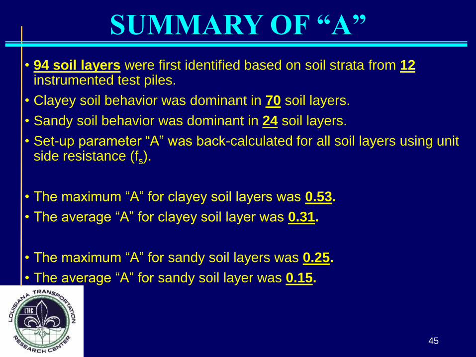
• 94 soil layers were first identified based on soil strata from 12 instrumented test piles.
• Clayey soil behavior was dominant in 70 soil layers.
• Sandy soil behavior was dominant in 24 soil layers.
• Set-up parameter “A” was back-calculated for all soil layers using unit side resistance (fs).
• The maximum “A” for clayey soil layers was 0.53.
• The average “A” for clayey soil layer was 0.31.
• The maximum “A” for sandy soil layers was 0.25.
• The average “A” for sandy soil layer was 0.15.
45

EMPIRICAL MODEL
46

Steps Followed for Model Preparation Identify potential soil properties
Find the correlation between soil properties and “A” parameter
Develop the model with SAS
Perform “F” test and “t” test to find the significance of the model as well the independent parameters
Perform detail statistical analyses (Goodness of fit, COV, Correlation among the parameters, Pseudo R
2 etc)
Validate the model with non-instrumented pile (These were not used to develop the model)
Verify the model with published case studies
47
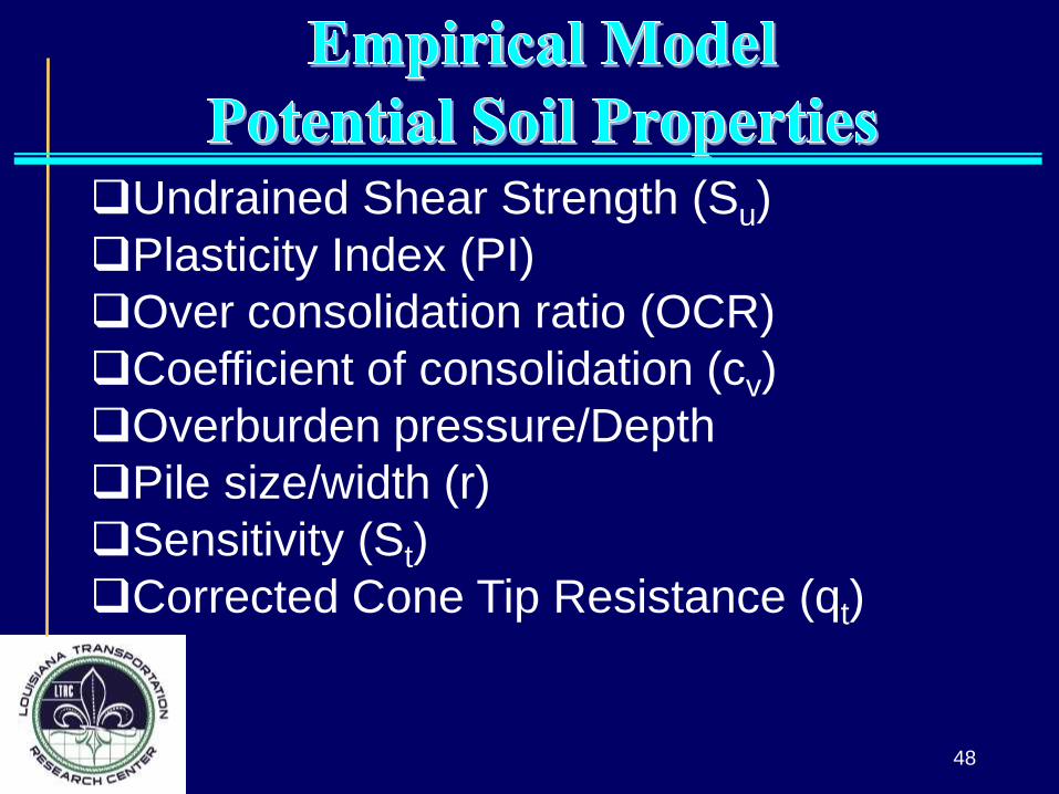
Undrained Shear Strength (Su)
Plasticity Index (PI)
Over consolidation ratio (OCR)
Coefficient of consolidation (cv)
Overburden pressure/Depth
Pile size/width (r)
Sensitivity (St)
Corrected Cone Tip Resistance (qt)
48

EMPIRICAL MODELS
Level-1 Including Undrained Shear Strength (Su)
Plasticity Index (PI)
Level-2 Including Undrained Shear Strength (Su)
Plasticity Index (PI)
Coefficient of Consolidation (cv)
Level-3 Including Undrained Shear Strength (Su)
Plasticity Index (PI)
Coefficient of Consolidation (cv)
Sensitivity (St)
49

Clayey soil with high Su exhibited low set-up
Clayey soil with low Su exhibited high set-up
Clayey soil with low PI exhibited low set-up
Clayey soil with high PI exhibited high set-up 50
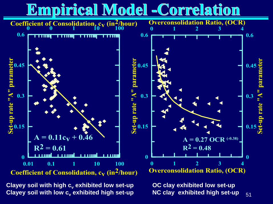
Clayey soil with high cv exhibited low set-up
Clayey soil with low cv exhibited high set-up
OC clay exhibited low set-up
NC clay exhibited high set-up 51
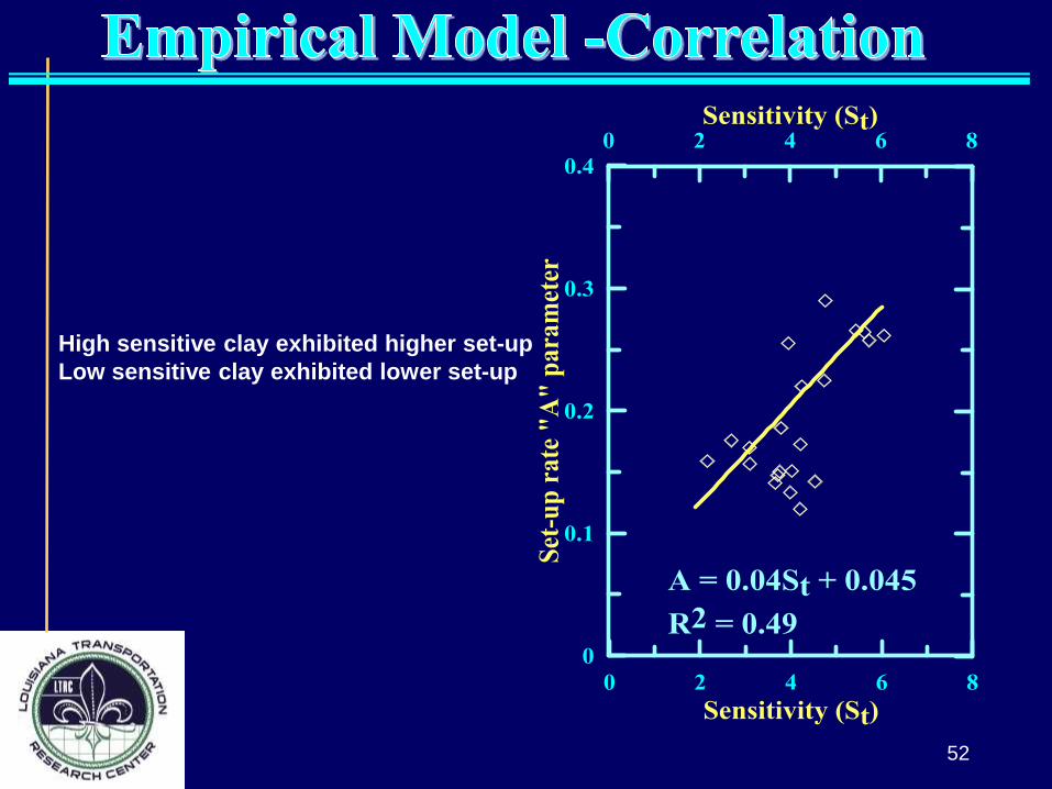
High sensitive clay exhibited higher set-up
Low sensitive clay exhibited lower set-up
52

No strong correlation was observed in
between depth and pile size with “r”
53

Final Developed Models
𝐀 =𝟏.𝟏𝟐∗
𝐏𝐈
𝟏𝟎𝟎+𝟎.𝟔𝟗
𝐒𝐮
𝟏𝐭𝐬𝐟𝟏
.𝟒𝟒 ∗ 𝐥𝐨𝐠
𝐂𝐯
𝟎.𝟎𝟏𝐢𝐧𝟐
𝐡𝐨𝐮𝐫
𝟎.𝟓𝟒+𝟑.𝟏𝟗
A=f (PI, Su, Cv)
𝑨 =𝟎.𝟕𝟗∗
𝑷𝑰
𝟏𝟎𝟎+𝟎.𝟒𝟗
𝑺𝒖
𝟏𝒕𝒔𝒇𝟐
.𝟎𝟑+𝟐.𝟐𝟕
A=f (PI, Su)
𝐀 =𝟎.𝟒𝟒∗
𝐏𝐈
𝟏𝟎𝟎𝐒
𝐭+𝟐.𝟐𝟎
𝐒𝐮
𝟏𝐭𝐬𝐟𝟏
.𝟗𝟒 ∗ 𝐥𝐨𝐠
𝐂𝐯
𝟎.𝟎𝟏𝐢𝐧
𝟐
𝐡𝐨𝐮𝐫
𝟏.𝟎𝟔+𝟏𝟎.𝟔𝟓
A=f (PI, Su, Cv, St)
54
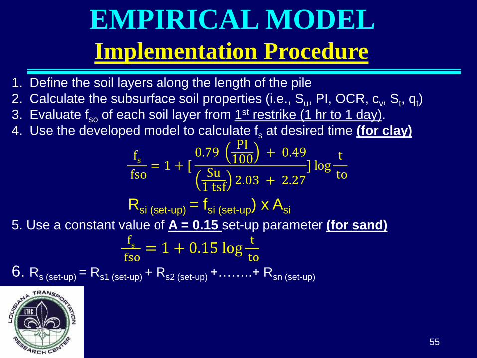
EMPIRICAL MODEL Implementation Procedure
1. Define the soil layers along the length of the pile
2. Calculate the subsurface soil properties (i.e., Su, PI, OCR, cv, St, qt)
3. Evaluate fso of each soil layer from 1st restrike (1 hr to 1 day).
4. Use the developed model to calculate fs at desired time (for clay)
fs
fso= 1 + [
0.79 PI
100 + 0.49
Su1 tsf
2.03 + 2.27] log
t
to
Rsi (set-up) = fsi (set-up) x Asi
5. Use a constant value of A = 0.15 set-up parameter (for sand)
f
s
fso= 1 + 0.15 log
t
to
6. Rs (set-up) = Rs1 (set-up) + Rs2 (set-up) +……..+ Rsn (set-up)
55

LRFD CALIBRATION
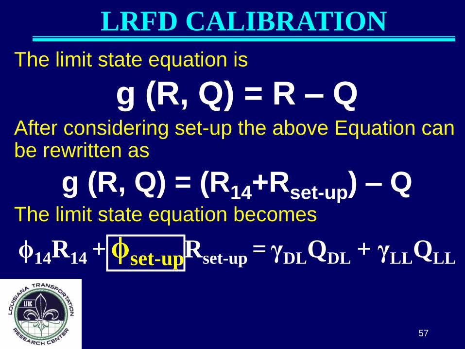
LRFD CALIBRATION
The limit state equation is
g (R, Q) = R – Q After considering set-up the above Equation can be rewritten as
g (R, Q) = (R14+Rset-up) – Q The limit state equation becomes
ϕ14R14 + ϕset-upRset-up = γDLQDL + γLLQLL
57

LRFD CALIBRATION For Φ14 By Abu-Farsakh et al. (2009)
Design Method
Resistance Factor (f14) and Efficiency Factor
(f/l) for Louisiana Soil Recommended
f14 FOSM FORM Monte Carlo
Simulation
f14 f14/l f14 f14/l f14 f14/l
Static method
a-Tomlinson
method and
Nordlund
method
0.56 0.58 0.63 0.66 0.63 0.66 0.60
Direct CPT
method
Schmertmann 0.44 0.47 0.48 0.52 0.49 0.53 0.48
LCPC/LCP 0.54 0.51 0.60 0.56 0.59 0.56 0.58
De Ruiter and
Beringen 0.66 0.55 0.74 0.62 0.73 0.61 0.70
CPT average 0.55 0.53 0.61 0.59 0.62 0.59 0.60
Dynamic
measurement
CAPWAP
(EOD) 1.31 0.36 1.41 0.39 — — 1.40
CAPWAP (14
days BOR) 0.55 0.44 0.61 0.52 0.62 0.47 0.60
58
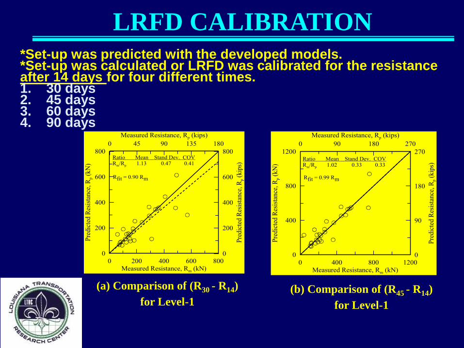
LRFD CALIBRATION
(a) Comparison of (R30 - R14)
for Level-1 (b) Comparison of (R45 - R14)
for Level-1
*Set-up was predicted with the developed models. *Set-up was calculated or LRFD was calibrated for the resistance after 14 days for four different times. 1. 30 days 2. 45 days 3. 60 days 4. 90 days
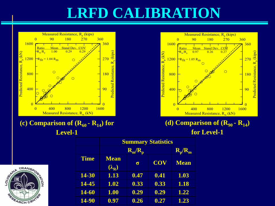
LRFD CALIBRATION
(c) Comparison of (R60 - R14) for
Level-1
(d) Comparison of (R90 - R14)
for Level-1
Summary Statistics
Rm/Rp Rp/Rm
Time Mean
(λR) σ COV Mean
14-30 1.13 0.47 0.41 1.03
14-45 1.02 0.33 0.33 1.18
14-60 1.00 0.29 0.29 1.22
14-90 0.97 0.26 0.27 1.23

Probability Density Function and Histogram
R30 - R14 R45 - R14
R60 - R14 R90 - R14
61
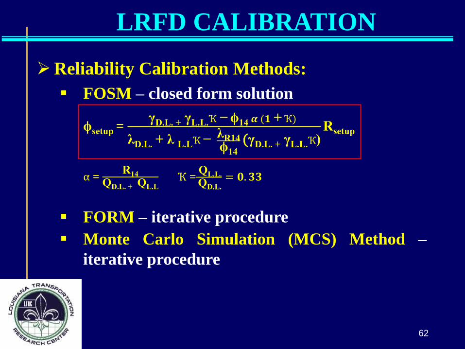
Reliability Calibration Methods:
FOSM – closed form solution
ϕsetup = γD.L. +
γL.L.Ҡ − ϕ14 𝜶 (𝟏 + Ҡ)
λD.L. + λ L.LҠ − λR14ϕ14
(γD.L. + γL.L.Ҡ)
Rsetup
FORM – iterative procedure
Monte Carlo Simulation (MCS) Method –
iterative procedure
62
α = R14
QD.L. + QL.L
Ҡ = QL.L.
QD.L.
= 𝟎. 𝟑𝟑
LRFD CALIBRATION
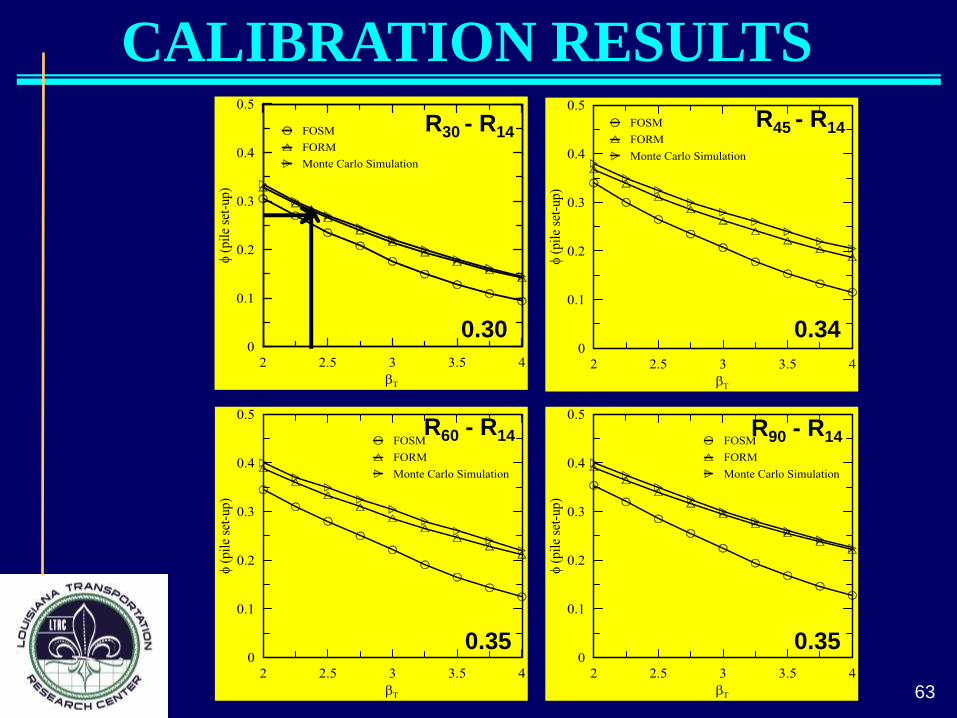
CALIBRATION RESULTS
R30 - R14 R45 - R14
R60 - R14 R90 - R14
0.30 0.34
0.35 0.35
63

βT = 2.33
Recommended FOSM FORM MC
LTRC @ 14-30 Days 0.28 0.28 0.30 0.30
LTRC @ 14-45 Days 0.32 0.33 0.34 0.34
LTRC @ 14-60 Days 0.34 0.35 0.36 0.35
LTRC @ 14-90 Days 0.34 0.36 0.37 0.35
Kam Ng (2013) 0.36 - -
Yang & Liang (2006) - 0.30 -
Overall Recommended = fsetup = 0.35
setupsetup1414LLDD RRQQ ff
64
CALIBRATION RESULTS

• Set-up study was conducted on 12 instrumented test piles of 5 different sites. Set-up was mainly exhibited by side resistance. The tip resistance was almost constant.
• Set-up was mainly attribute to the consolidation behavior. Amount of set-up and set-up rate increased significantly during consolidation phase. Very small amount of set-up was observed during “aging” period.
• Horizontal effective stress increased significantly during the consolidation period. Once the consolidation period was over, the amount of increase became slower.
• Set-up for individual soil layers was calculated with the aid of strain gauge.
• The set-up rate “A” for clayey soil layers was 0.31 and for sandy soil layers it was 0.15.
65
CONCLUSIONS
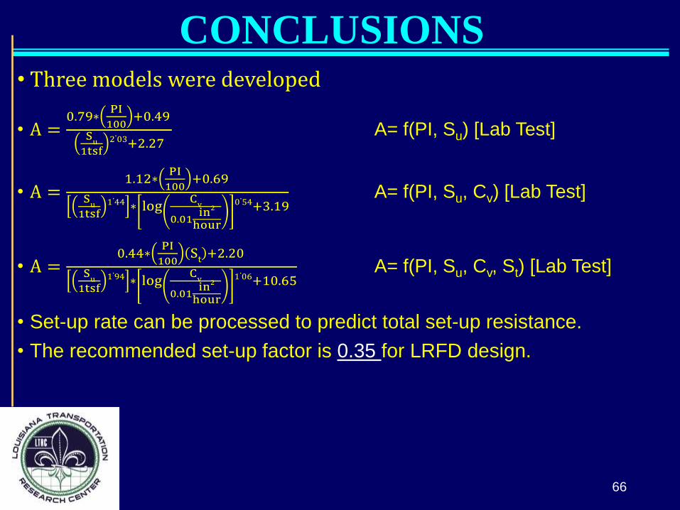
• Three models were developed
• A =0.79∗
PI
100+0.49
Su
1tsf2
.03+2.27
A= f(PI, Su) [Lab Test]
• A =1.12∗
PI
100+0.69
Su
1tsf1
.44 ∗ log
Cv
0.01in2
hour
0.54+3.19
A= f(PI, Su, Cv) [Lab Test]
• A =0.44∗
PI
100S
t+2.20
Su
1tsf1
.94 ∗ log
Cv
0.01in2
hour
1.06+10.65
A= f(PI, Su, Cv, St) [Lab Test]
• Set-up rate can be processed to predict total set-up resistance.
• The recommended set-up factor is 0.35 for LRFD design.
66
CONCLUSIONS
67
• Chen, Q., Haque, Md. N., Abu-Farsakh, M., and Fernandez, B. A. (2014). “Field investigation of pile setup in mixed soil.” Geotechnical Testing Journal, Vol. 37(2), pp. 268-281.
• Haque, Md. N., Abu-Farsakh, M., Chen, Q., and Zhang, Z. (2014). “A case study on instrumenting and testing full scale test piles for evaluating set-up phenomenon.” Journal of the Transportation Research Board No 2462, National Research Council, Washington, D.C., pp. 37-47.
• Haque, Md. N., Abu-Farsakh, M., Zhang, Z. and Okeil, A. (2016). “Estimate pile set-up for individual soil layers and develop a model to estimate the increase in unit side resistance with time based on PCPT data.” Journal of the Transportation Research Board , National Research Council, Washington, D.C. (In Press).
• Haque, Md. N., Chen, Q., Abu-Farsakh, M., and Tsai, C. (2014). “Effects of pile size on set-up behavior of cohesive soils.” In Proceedings of Geo-Congress-2014: Geo-Characterization and Modeling for Sustainability, Technical Papers GSP 234, pp. 1743-1749.
• Haque, Md. N., Abu-Farsakh, M., and Chen, Q. (2015). “Pile set-up for individual soil layers along instrumented test piles in clayey soil.” In Proceedings of the 15th Pan-American Conference on Soil Mechanics and Geotechnical Engineering (From fundamentals to applications in Geotechnics), November 15-18, Argentina, pp. 390-397.

68
ACKNOWLEDGEMENT
• LADOTD Geotechnical Department
• Louisiana Transportation Research Center (LTRC)