February 8 th, 2001 Status Report: SciFi for MICE Edward McKigney Imperial College London.

How well targeted are soda taxes?
Pierre Dubois, Rachel Griffith and Martin O’Connell
Institute for Fiscal Studies
Imperial, February 2018
1 / 28
Motivation
I Sugar consumption is far in excess of recommended levels across muchof the developed world Detail
I Eating too much sugar is associated with externalities
I diet related disease (e.g. obesity, type II diabetes)
I too much sugar early in life is associated with poorer long run outcomes
I Consumption of soda has been highlighted as a major driver of highlevels of dietary sugar, particularly in young
I Corrective tax can help off-set these externalities
2 / 28
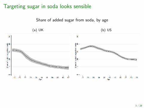
Targeting sugar in soda looks sensible
(a) UK (b) US
3 / 28
Share of added sugar from soda, by age
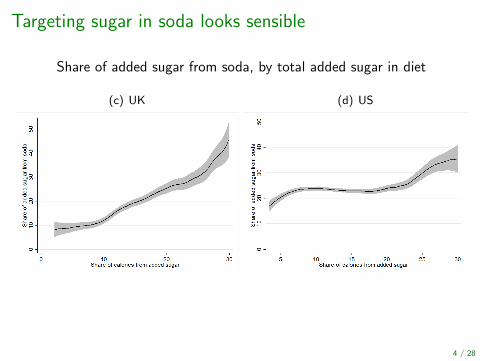
Targeting sugar in soda looks sensible
(c) UK (d) US
4 / 28
Share of added sugar from soda, by total added sugar in diet
Our contribution
I How effective soda taxes are in changing sugar consumption of thetargeted population
I we estimate consumer demand in the UK drinks market
I and simulate impact of tax, accounting for pass-through
I Relative to existing work, we
I study on-the-go purchases for immediate consumption
I consumption of soda out of the home is very common (≈50%)
I data include purchases of teenagers
I longitudinal data allows estimation of individual level preferencesrelaxing common restrictions on preference structures
5 / 28
Outline
1. Motivation and contribution
2. Demand model
3. On-the-go data
4. Demand estimates
5. Soda tax simulation
6. Summary and conclusions
6 / 28
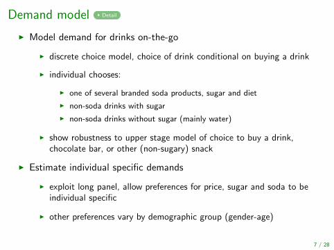
Demand model Detail
I Model demand for drinks on-the-go
I discrete choice model, choice of drink conditional on buying a drink
I individual chooses:
I one of several branded soda products, sugar and diet
I non-soda drinks with sugar
I non-soda drinks without sugar (mainly water)
I show robustness to upper stage model of choice to buy a drink,chocolate bar, or other (non-sugary) snack
I Estimate individual specific demands
I exploit long panel, allow preferences for price, sugar and soda to beindividual specific
I other preferences vary by demographic group (gender-age)
7 / 28
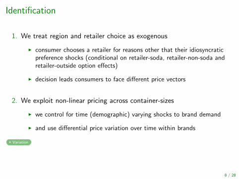
Identification
1. We treat region and retailer choice as exogenous
I consumer chooses a retailer for reasons other that their idiosyncraticpreference shocks (conditional on retailer-soda, retailer-non-soda andretailer-outside option effects)
I decision leads consumers to face different price vectors
2. We exploit non-linear pricing across container-sizes
I we control for time (demographic) varying shocks to brand demand
I and use differential price variation over time within brands
Variation
8 / 28
Outline
1. Motivation and contribution
2. Demand model
3. On-the-go data
4. Demand estimates
5. Soda tax simulation
6. Summary and conclusions
9 / 28

Data
I Around 50% of soda is purchased and consumed outside the home
I We use novel data on food and drink purchases made on-the-go(collected by Kantar in the UK)
I Individuals record, at barcode level, all purchases from stores andvending machines
I Participants belong to households in the Kantar Worldpanel
I records all grocery purchases made and brought into the home
I means we have measures of overall household spending and diet forindividuals in our sample
I Sample of 5,400 individuals from June 2009-October 2012
I observe each person making a food/drink purchase on at least 25 days
I and 81 on average
10 / 28

Consumer age
Age group13-22 22-30 31-40 41-50 51-60 60+
% of sample 9 14 22 23 18 14
% of groupthat ever 0.68 0.67 0.66 0.59 0.49 0.38purchases soda
Sugar from soda (g) 1754 1439 1181 1235 1054 886
11 / 28

Total dietary sugar
Decile of distribution of share of calories from added sugar1 2 3 4 5 6 7 8 9 10
% of groupthat ever 0.46 0.53 0.52 0.56 0.58 0.59 0.61 0.63 0.63 0.67purchases soda
Sugar from 797 962 951 892 1037 1053 1175 1095 1298 1832soda (g)
12 / 28
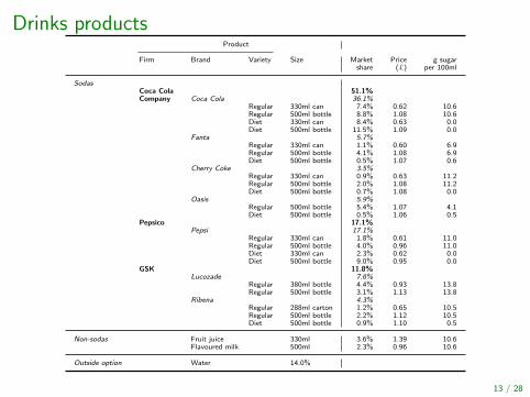
Drinks productsProduct
Firm Brand Variety Size Market Price g sugarshare (£) per 100ml
SodasCoca Cola 51.1%Company Coca Cola 36.1%
Regular 330ml can 7.4% 0.62 10.6Regular 500ml bottle 8.8% 1.08 10.6Diet 330ml can 8.4% 0.63 0.0Diet 500ml bottle 11.5% 1.09 0.0
Fanta 5.7%Regular 330ml can 1.1% 0.60 6.9Regular 500ml bottle 4.1% 1.08 6.9Diet 500ml bottle 0.5% 1.07 0.6
Cherry Coke 3.5%Regular 330ml can 0.9% 0.63 11.2Regular 500ml bottle 2.0% 1.08 11.2Diet 500ml bottle 0.7% 1.08 0.0
Oasis 5.9%Regular 500ml bottle 5.4% 1.07 4.1Diet 500ml bottle 0.5% 1.06 0.5
Pepsico 17.1%Pepsi 17.1%
Regular 330ml can 1.8% 0.61 11.0Regular 500ml bottle 4.0% 0.96 11.0Diet 330ml can 2.3% 0.62 0.0Diet 500ml bottle 9.0% 0.95 0.0
GSK 11.8%Lucozade 7.6%
Regular 380ml bottle 4.4% 0.93 13.8Regular 500ml bottle 3.1% 1.13 13.8
Ribena 4.3%Regular 288ml carton 1.2% 0.65 10.5Regular 500ml bottle 2.2% 1.12 10.5Diet 500ml bottle 0.9% 1.10 0.5
Non-sodas Fruit juice 330ml 3.6% 1.39 10.6Flavoured milk 500ml 2.3% 0.96 10.6
Outside option Water 14.0%
13 / 28
Outline
1. Motivation and contribution
2. Demand model
3. On-the-go data
4. Demand estimates
5. Soda tax simulation
6. Summary and conclusions
14 / 28

Marginal preference distributions Bivariate Coefficients
(a) Price (b) Sugar
(c) Soda
15 / 28
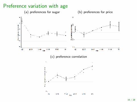
Preference variation with age(a) preferences for sugar (b) preferences for price
(c) preference correlation
16 / 28

Preference variation with total dietary sugar(a) preferences for sugar (b) preferences for price
(c) preference correlation
Coefficients
17 / 28
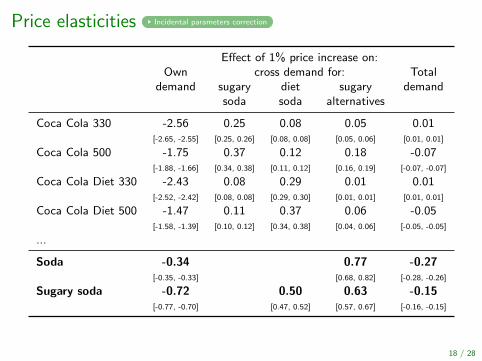
Price elasticities Incidental parameters correction
Effect of 1% price increase on:Own cross demand for: Total
demand sugary diet sugary demandsoda soda alternatives
Coca Cola 330 -2.56 0.25 0.08 0.05 0.01[-2.65, -2.55] [0.25, 0.26] [0.08, 0.08] [0.05, 0.06] [0.01, 0.01]
Coca Cola 500 -1.75 0.37 0.12 0.18 -0.07[-1.88, -1.66] [0.34, 0.38] [0.11, 0.12] [0.16, 0.19] [-0.07, -0.07]
Coca Cola Diet 330 -2.43 0.08 0.29 0.01 0.01[-2.52, -2.42] [0.08, 0.08] [0.29, 0.30] [0.01, 0.01] [0.01, 0.01]
Coca Cola Diet 500 -1.47 0.11 0.37 0.06 -0.05[-1.58, -1.39] [0.10, 0.12] [0.34, 0.38] [0.04, 0.06] [-0.05, -0.05]
...
Soda -0.34 0.77 -0.27[-0.35, -0.33] [0.68, 0.82] [-0.28, -0.26]
Sugary soda -0.72 0.50 0.63 -0.15[-0.77, -0.70] [0.47, 0.52] [0.57, 0.67] [-0.16, -0.15]
18 / 28
Outline
1. Motivation and contribution
2. Demand model
3. On-the-go data
4. Demand estimates
5. Soda tax simulation
6. Summary and conclusions
19 / 28
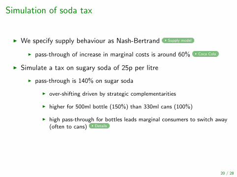
Simulation of soda tax
I We specify supply behaviour as Nash-Bertrand Supply model
I pass-through of increase in marginal costs is around 60% Coca Cola
I Simulate a tax on sugary soda of 25p per litre
I pass-through is 140% on sugar soda
I over-shifting driven by strategic complementarities
I higher for 500ml bottle (150%) than 330ml cans (100%)
I high pass-through for bottles leads marginal consumers to switch away(often to cans) Details
20 / 28

Impact of tax on equilibrium prices and shares
Sugary Diet Sugary Outsidesoda soda alternatives option
Tax (pence) 10.55 0.00 0.00 0.00
∆ price (pence) 14.98 -3.12 0.00 0.00[14.05, 15.90] [-3.66, -2.58]
∆ share (p.p.) -5.50 3.41 0.59 1.51[-5.48, -4.96] [2.92, 3.30] [0.53, 0.62] [1.45, 1.59]
21 / 28
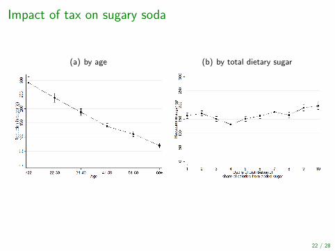
Impact of tax on sugary soda
(a) by age (b) by total dietary sugar
22 / 28
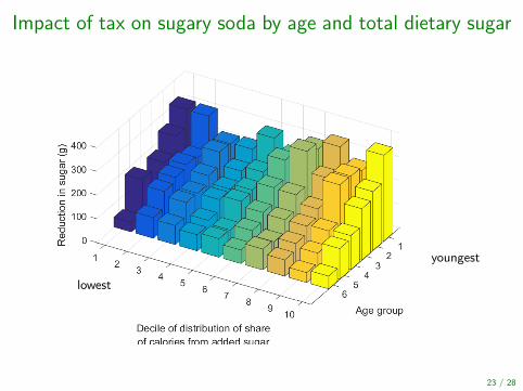
Impact of tax on sugary soda by age and total dietary sugar
23 / 28
youngest
lowest
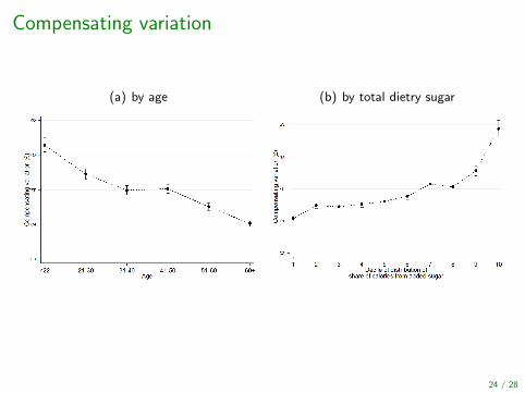
Compensating variation
(a) by age (b) by total dietry sugar
24 / 28
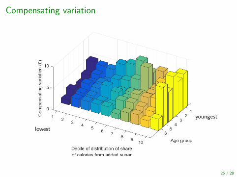
Compensating variation
25 / 28
youngest
lowest
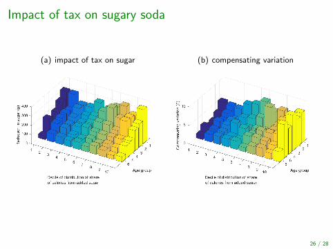
Impact of tax on sugary soda
(a) impact of tax on sugar (b) compensating variation
26 / 28
Consumer welfare
I We want to weight compensating variation against benefits fromreduced consumption
I Size of externalities, and costs from excess consumption that fall onthe consumer themselves are very difficult to measure
I We can compute average saving that would be necessary to makeconsumers indifferent to tax
I e.g. per can of Coca Cola
I £0.80 for those aged below 22
I £1.40 for those in top decile of dietary sugar distribution
By income Robustness
27 / 28
Summary
I We estimate consumer specific preferences on-the-go for drinks
I Approach captures arbitrary relationship between tax predictions andindividual attributes
I We show a tax on sugary soda is well targeted at young
I because of the correlation between sugar preferences and price sensitivefor young consumers
I But less effective at targeting older consumers with high levels of totaldietary sugar
I because of the lack of correlation between sugar preferences and pricesensitive for older heavy sugar consumers
28 / 28

EXTRA SLIDES

Share of total calories from added sugar Back
(c) US (d) UK
28 / 28
65% of people are above10% calories from added sugar
(recommended max in US)
70% are above 10%
90% are above 5%(recommended max in UK)
Source: NHANES (US), LCFS (UK)

Demand model Back
I Consumers, i = 1, . . . ,N, choose which drink to purchase (whileon-the-go)
I We observe each consumer on many choice occasions, t = 1, . . . ,T
I Products include j = 0, . . . , J
I sugary sodas
I diet sodas
I alternative drinks such as fruit juice or flavoured milk
I the outside option (bottled water) i
I Each product j belongs to a brand b(j)
I Each consumer i belongs to demographic (age-sex) group d(i)
28 / 28
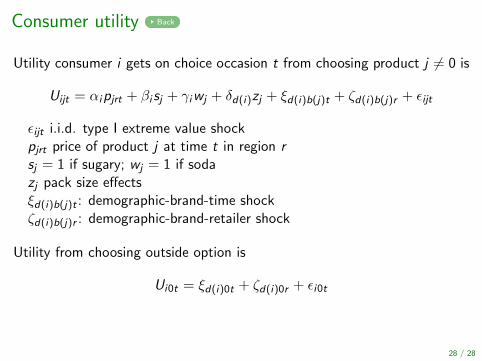
Consumer utility Back
Utility consumer i gets on choice occasion t from choosing product j 6= 0 is
Uijt = αipjrt + βi sj + γiwj + δd(i)zj + ξd(i)b(j)t + ζd(i)b(j)r + εijt
εijt i.i.d. type I extreme value shockpjrt price of product j at time t in region rsj = 1 if sugary; wj = 1 if sodazj pack size effectsξd(i)b(j)t : demographic-brand-time shockζd(i)b(j)r : demographic-brand-retailer shock
Utility from choosing outside option is
Ui0t = ξd(i)0t + ζd(i)0r + εi0t
28 / 28
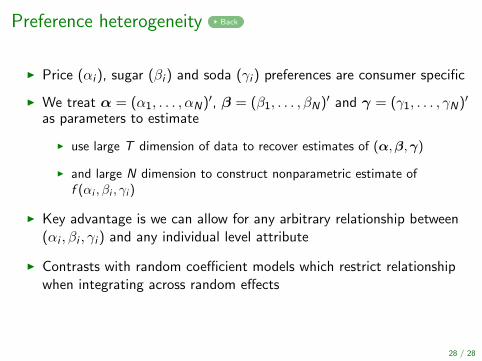
Preference heterogeneity Back
I Price (αi ), sugar (βi ) and soda (γi ) preferences are consumer specific
I We treat α = (α1, . . . , αN)′, β = (β1, . . . , βN)′ and γ = (γ1, . . . , γN)′
as parameters to estimate
I use large T dimension of data to recover estimates of (α,β,γ)
I and large N dimension to construct nonparametric estimate off (αi , βi , γi )
I Key advantage is we can allow for any arbitrary relationship between(αi , βi , γi ) and any individual level attribute
I Contrasts with random coefficient models which restrict relationshipwhen integrating across random effects
28 / 28
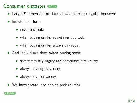
Consumer distastes Back
I Large T dimension of data allows us to distinguish between:
I Individuals that:
I never buy soda
I when buying drinks, sometimes buy soda
I when buying drinks, always buy soda
I And individuals that, when buying soda:
I sometimes buy sugary and sometimes diet variety
I always buy sugary variety
I always buy diet variety
I We incorporate into choice probabilities
Details
28 / 28

Choice probabilities Back
I For a consumer we observe buying sugary soda, diet soda and anon-soda drink
I She chooses between the set of sodas and non-sodas, Ωi = Ωa
⋃Ωn
I And has a finite sugar and soda preference
I For this consumer the choice probability for j 6= 0 is:
Pit(j) =exp(αipjrt + βi sj + γiwj + ηijrt)
exp(ξd(i)0t + ζd(i)0r ) +∑
k∈Ωiexp(αipjrt + βi sj + γiwj + ηikrt)
where ηijrt = δd(i)zj + ξd(i)b(j)t + ζd(i)b(j)r
28 / 28

Choice probabilities Back
I For a consumer we observe buying sugary soda, a non-soda drink butno diet soda
I She chooses between the set of sugary sodas and non-sodas,Ωi = Ωs
⋃Ωn
I And has a finite soda preference, but negatively infinite preference fordiet
I For this consumer the choice probability for j 6= 0 is:
Pit(j) =exp(αipjrt + γiwj + ηijrt)
exp(ξd(i)0t + ζd(i)0r ) +∑
k∈Ωiexp(αipjrt + γiwj + ηikrt)
where ηijrt = δd(i)zj + ξd(i)b(j)t + ζd(i)b(j)r
28 / 28

Price variation of Coca Cola Back
(a) 330ml can (b) 500ml bottle
(c) Within brand price variation
28 / 28
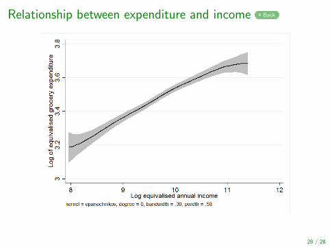
Relationship between expenditure and income Back
28 / 28

Coefficient estimates - consumer specific Back
Moments of distribution of consumer specific preferences
Estimate StandardVariable error
Price Mean -2.8349 0.0728Standard deviation 3.0401 0.0480Skewness -1.4532 0.1051Kurtosis 5.8163 0.6329
Soda Mean 0.1490 0.0965Standard deviation 2.3738 0.0387Skewness 1.2065 0.0815Kurtosis 5.0141 0.3733
Sugar Mean 0.0550 0.0164Standard deviation 1.8340 0.0194Skewness -0.0014 0.0606Kurtosis 3.9429 0.2341
Price-Soda Covariance -5.6252 0.3427Price-Sugar Covariance -1.0102 0.2236Soda-Sugar Covariance 0.4631 0.2928
28 / 28
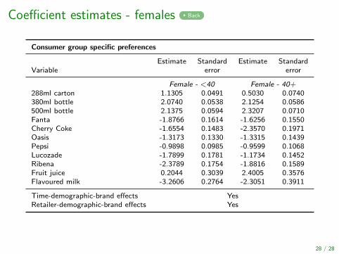
Coefficient estimates - females Back
Consumer group specific preferences
Estimate Standard Estimate StandardVariable error error
Female - <40 Female - 40+288ml carton 1.1305 0.0491 0.5030 0.0740380ml bottle 2.0740 0.0538 2.1254 0.0586500ml bottle 2.1375 0.0594 2.3207 0.0710Fanta -1.8766 0.1614 -1.6256 0.1550Cherry Coke -1.6554 0.1483 -2.3570 0.1971Oasis -1.3173 0.1330 -1.3315 0.1439Pepsi -0.9898 0.0985 -0.9599 0.1068Lucozade -1.7899 0.1781 -1.1734 0.1452Ribena -2.3789 0.1754 -1.8816 0.1589Fruit juice 0.2044 0.3039 2.4005 0.3576Flavoured milk -3.2606 0.2764 -2.3051 0.3911
Time-demographic-brand effects YesRetailer-demographic-brand effects Yes
28 / 28
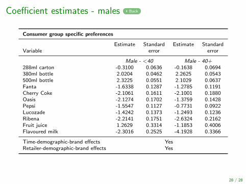
Coefficient estimates - males Back
Consumer group specific preferences
Estimate Standard Estimate StandardVariable error error
Male - <40 Male - 40+288ml carton -0.3100 0.0636 -0.1638 0.0694380ml bottle 2.0204 0.0462 2.2625 0.0543500ml bottle 2.3225 0.0551 2.1029 0.0637Fanta -1.6338 0.1287 -1.2785 0.1191Cherry Coke -2.1061 0.1611 -2.1001 0.1880Oasis -2.1274 0.1702 -1.3759 0.1428Pepsi -1.5547 0.1127 -0.7731 0.0922Lucozade -1.4242 0.1373 -1.2493 0.1236Ribena -2.2141 0.1751 -2.6324 0.2162Fruit juice 1.2629 0.3314 -1.1853 0.4006Flavoured milk -2.3016 0.2525 -4.1928 0.3366
Time-demographic-brand effects YesRetailer-demographic-brand effects Yes
28 / 28
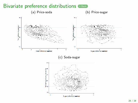
Bivariate preference distributions Back
(a) Price-soda (b) Price-sugar
(c) Soda-sugar
28 / 28
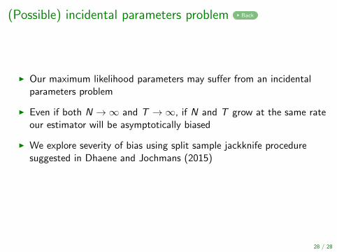
(Possible) incidental parameters problem Back
I Our maximum likelihood parameters may suffer from an incidentalparameters problem
I Even if both N →∞ and T →∞, if N and T grow at the same rateour estimator will be asymptotically biased
I We explore severity of bias using split sample jackknife proceduresuggested in Dhaene and Jochmans (2015)
28 / 28
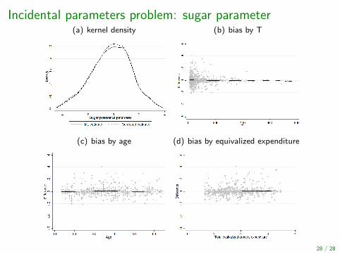
Incidental parameters problem: sugar parameter(a) kernel density (b) bias by T
(c) bias by age (d) bias by equivalized expenditure
28 / 28
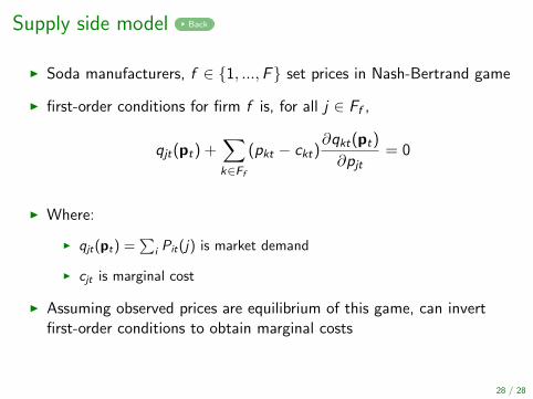
Supply side model Back
I Soda manufacturers, f ∈ 1, ...,F set prices in Nash-Bertrand game
I first-order conditions for firm f is, for all j ∈ Ff ,
qjt(pt) +∑k∈Ff
(pkt − ckt)∂qkt(pt)
∂pjt= 0
I Where:
I qjt(pt) =∑
i Pit(j) is market demand
I cjt is marginal cost
I Assuming observed prices are equilibrium of this game, can invertfirst-order conditions to obtain marginal costs
28 / 28

Volumetric sugary soda tax Back
I Simulate impact of tax of 25p per litre (τ = 0.25) on sugary soda
pjt =
pjt + τ ljpjt
∀j ∈ Ωs
∀j ∈ Ωd⋃
Ωn
I Vector of equilibrium producer prices, pjt , for all firms, satisfy
qjt(pt) +∑k∈Ff
(pkt − ckt)∂qkt(pt)
∂pjt= 0 ∀j ∈ Ff
28 / 28

Pass-through of marginal cost shock Back
Pass-through(%)
Coca Cola 330 22Coca Cola 500 72Coca Cola Diet 330 24Coca Cola Diet 500 84Fanta 330 20Fanta 500 74Fanta Diet 500 101Cherry Coke 330 23Cherry Coke 500 69Cherry Coke Diet 500 82Oasis 500 75Oasis Diet 500 97
28 / 28
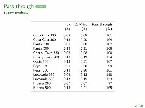
Pass-through Back
Sugary products
Tax ∆ Price Pass-through(£) (£) (%)
Coca Cola 330 0.08 0.08 101Coca Cola 500 0.13 0.20 164Fanta 330 0.08 0.08 102Fanta 500 0.13 0.21 168Cherry Coke 330 0.08 0.08 100Cherry Coke 500 0.13 0.19 154Oasis 500 0.13 0.21 167Pepsi 330 0.08 0.08 99Pepsi 500 0.13 0.20 161Lucozade 380 0.09 0.13 140Lucozade 500 0.13 0.19 153Ribena 288 0.07 0.07 97Ribena 500 0.13 0.21 165
28 / 28
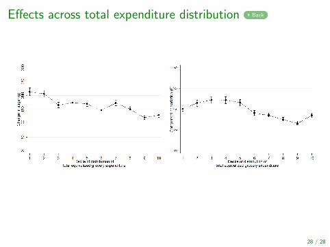
Effects across total expenditure distribution Back
28 / 28

Switching to sugar in food Back
I A possible consequence of a soda tax is people switch to sugar in food
I We consider a two-stage choice model
I stage one: choose from a set of confectionery products, or a non sugarysnack, or to opt for a drink
I stage two: if drink is chosen in stage one, decide which one to select
I Full preferences heterogeneity we estimate in stage two influencesstage one
I Simplifying assumption is idiosyncratic drinks shocks not known atstage one
I For soda consumers, implies sugar reductions is 4% (for age< 22) to11% (for age 51-60) smaller
28 / 28