Master of Science in Petroleum Engineering. . - ............................ _ ......... { „ ......‘sfe# . . . *

PETROLEUM GEOLOGY

D r M . A I a

,

Imperial College.ondon

Centre for Petroleum StudiesDepartm ent of Earth Science and EngineeringRoyal School of M ines BuildingPrince Consort RoadLondon SW 7 2AZUnited Kingdom

C O N T E N T SPAGE

1. INTRODUCTION: RESERVOIR FLUID AND ROCK PROPERTIES..................................... 4

FLUID DISTRIBUTION IN A RESEVOIR...................................................... ........... 4

WETNESS.................................................................................................................... 4

RESERVOIR ROCK PROPERTIES........................................................................... 5

POROSITY..................................................................................................... .......5

PERMEABILITY.............................................................................. ...................... 7

PORE GEOMETRY..................................................... .........................................8

OBJECTIVES OF WIRELINE LOGGING.,.......................................................................9

Qualitative Interpretation........................................................................................9

Quantitative Interpretation.... ................................................................................9

THE BOREHOLE ENVIRONMENT: INVASION EFFECTS..........................................10

MATRIX CONCEPT.........................................................................................................12

DATA ACQUISITION ...................................................................................................... 13

LOG DATA RECORDING FORMAT ..............................................................................19

TYPES OF LOGS ............................................................................................................20

NOMENCLATURE............................................................................................................20

2. ELECTRIC LOGS.....................................................................................................................24

THE SP LOG.....................................................................................................................24

RESISTIVITY LOGS................................................................. .......................................33

INVASION AND RESISTIVITY PROFILES....................................................................35

RESISTIVITY MEASUREMENT............................................................................. .......41

RECENT ADVANCES IN RESISTIVITY LOGGING............................................... 50

QUALITATIVE INTERPRETATION OF ELECTRIC LOGS............................................ 57

3. THE BOREHOLE COMPENSATED (BHC) SONIC LOG............................................... ......60

LONG SPACING SONIC TOOL (LSS)...........................................................................69

THE ARRAY SONIC TOOL (AST)...................................................................................69

DETECTION OF ABNORMAL PRESSURES................... ............................................. 73

4. RADIOACTIVE LOGS 76

THE GAMMA RAY (GR) LOG .................................................................................. 77

THE NATURAL GAMMA RAY SPECTROMETRY TOOL (NGS).................................80

THE NEUTRON LOG ................................................................ ................................... 87

THE FORMATION DENSITY COMPENSATED (FDC) LOG ..................................... 93

THE LITHO-DENSITY LOG.................................................................. ..........................98

DETECTION OF ABNORMAL PRESSURES................................................... ...........103

5. THE ELECTROMAGNETIC PROPAGATION TOOL (EPT LOG) ....................................104

6. THE NUCLEAR MAGNETIC RESONANCE LOG (NMR)................................................... 113

7. PLATFORM EXPRESS (PEX)............................................................................................... 126>

8. LOG INTERPRETATION.............................................................. ...... ........... ..................... 132

QUALITATIVE INTERPRETATION ............................................................................ 133

WIRE LINE LOG CHARACTERISTICS OF POTENTIAL SOURCE ROCKS..... 135

QUANTITATIVE INTERPRETATION ......................................................................... 144

9. SHALY FORMATION INTERPRETATION..........................................................................177

10. INTRODUCTION TO DIPMETER AND FORMATION IMAGE LOGS............................ 182

THE DIPMETER LOG.................................................................................................... 182

FORMATION IMAGE LOGS...... ................................................................................... 190

ELECTRICAL IMAGE TOOLS................................................................................... 190

ACOUSTIC (ULTRASONIC) IMAGE TOOLS...........................................................191

IMAGE INTERPRETATION...................................... ...................................... ...192

SELECTED REFERENCES ............................. ........................................................................ 198

EXERCISES 202

1. INTRODUCTION: RESERVOIR FLUID AND ROCK PROPERTIES

FLUID DISTRIBUTION IN A RESERVOIR

The distribution of the fluids in a reservoir rock is dependent on the densities of the fluids and

the capillary properties of the rock. Being the lightest, gas occupies the uppermost zone (the gas

cap), which is underlain, respectively, by oil and then water. In the uppermost zone the pores

are filled mainly by gas while in the middle zone the pores are occupied principally by oil with

gas in solution. In the lowermost zone the pores are filled by water. A certain amount of water

occurs along with the oil in the middle zone, the proportion often being of the order of 10 to 30

per cent. Moving upwards across the water-oil-contact in the reservoir, there is a gradual

increase in oil saturation accompanied by a progressive decrease water saturation, giving rise to

a transition zone from pores occupied entirely by water to pores occupied mainly by oil. The

thickness of this transition zone depends on the densities and interfacial tension between oil and

water, and on the sizes o£ the pores. A similar transition zone occurs between oil and gas when

moving upwards across the oil-gas contact: oil saturation gradually decreases while gas

saturation gradually increases. There is also some water in the pores in the gas zone. It should

therefore be noted that although drawn as sharp boundaries on maps and cross-sections, fluid

contacts are not in fact sharp lines. The so-called gas-oil and oil-water contacts are generally

horizontal. However, in certain circumstances these fluid contacts are inclined, usually only very

gently.

WETNESS

The water found in the oil and gas zones is known generally as interstitial water. This interstitial

water occurs as collars around grain contacts, as a filling of pores with unusually small throats

connecting with adjacent pores and to a much smaller extent as wetting films on the surface of

the mineral grains. This is illustrated Figure 1.1, which shows an enlarged section through a

granular rock.WATER GAS OR

COLLARS OIL

Fig 1.1 An enlarged section through a granular reservoir illustrating the distribution of water and hydrocarbons and wettability (After Hobson, 1984)

In this case the reservoir is said to be water wet, which means that the hydrocarbons are not in

direct contact with the grains that make up the reservoir. The mineral grains are coated by a thin

film water which intervenes between them and the hydrocarbons. The water film owes its

existence to a greater force of attraction between the liquid and the grain surfaces than the

cohesive strength of the liquid itself.

Oil can also be a wetting agent, but gas cannot act as a wetting fluid as its physical properties

do not allow it to form a coherent film around the mineral grains. However, gas reservoirs which

were previously oil filled could become oil wet.

Knowledge of the nature of the agent wetting a reservoir is important as it affects the production

behaviour of the reservoir. It must also be considered when designing secondary recovery

programmes. Preservation^ the reservoir wettability in cores is thus important if the subsequent

laboratory tests of electrical properties and fluid flow behaviour are to be truly representative of

the reservoir characteritics.

RESERVOIR ROCK PROPERTIES

The most important properties of a reservoir are its porosity (Ф) and permeability (k). Porosity

determines the storage capacity of the reservoir, while permeability governs its ability to transmit

fluids. These important characteristics are discussed briefly below.

POROSITY

Porosity is expressed as a percentage of the bulk volume of the rock:

Ф = (pore volume)/(bulk volume) X 100

The most common range is 10% - 20% and the highest recorded porosity value is 37%. The

maximum theoretical porosity value is 47%. Fluids occur in the pore spaces within the reservoir

(Fig 1.2).

Ф

1-ФFig1.2 Illustration of porosity and

matrix (After Schlumberger)

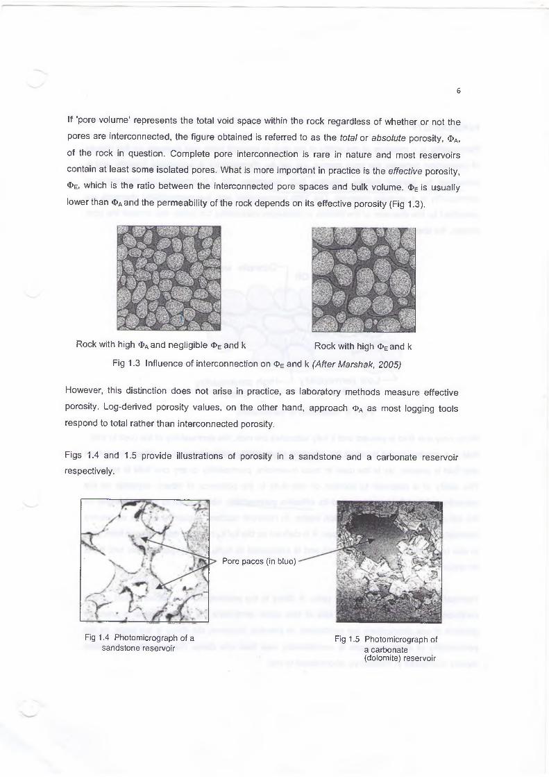
If ‘pore volume’ represents the total void space within the rock regardless of whether or not the

pores are interconnected, the figure obtained is referred to as the total or absolute porosity, ФА,

of the rock in question. Complete pore interconnection is rare in nature and most reservoirs

contain at least some isolated pores. What is more important in practice is the effective porosity,

ФЕ, which is the ratio between the interconnected pore spaces and bulk volume. ФЕ is usually

lower than ФAand the permeability of the rock depends on its effective porosity (Fig 1.3).

Rock with high ФА and negligible ФЕ and к Rock with high ФЕ and к

Fig 1.3 Influence of interconnection on ФЕ and к (After Marshak, 2005)

However, this distinction does not arise in practice, as laboratory methods measure effective

porosity. Log-derived porosity values, on the other hand, approach ФА as most logging tools

respond to total rather than interconnected porosity.

Figs 1.4 and 1.5 provide illustrations of porosity in a sandstone and a carbonate reservoir

respectively.

Pore paces (in blue)

Fig 1.4 Photomicrograph of a Fig 1.5 Photomicrograph ofsandstone reservoir a carbonate

(dolomite) reservoir

PERMEABILITY

Permeability is a measure of the ability of the rock to transmit fluids and depends on the degree

of connection between the pore spaces, i.e. ол Ф е - Permeability is a complex quantity and is>o, —- ----------- - ' '

influenced by several factors including flurd saturation. Fig 1.6 provides an illustration of

permeability in a granular reservoir. The ‘high permeability’ and ‘low permeability’ channels are

controlled by the diameter of the throats or passages connecting the pores: the smaller the pore

throats, the lower the permeability.

----- -- ---------------- . liyi< permeability pore channel------------ pore channel

Fig 1.6 Illustration of permeability

Sand grainsConnate water

When only one fluid is present and it fully saturates the rock, the permeability of the rock to that

fluid is a maximum and is called the absolute permeability, abbreviated to kA. When more than

one fluid is present, as is the case in most reservoirs, permeability to any one fluid is reduced.

The ability of a reservoir to conduct of one fluid in the presence of others depends on the

saturation of that fluid and is called its effective permeability, abbreviated to kE. kE changes as

the saturation of the fluid in question varies. In reservoir studies, a quantity known as relative

permeability, abbreviated to kr, is used. It is defined as the kE/ kA ratio, its value ranges from zero

to one (depending on fluid saturation) and is expressed as k0/kA for oil, kG/kA for gas and kw/kA

for water.

Permeability is expressed in darcy units. A darcy is the permeability that allows a fluid of one

centipoise viscosity to flow at the rate of one cubic centimetre per second under a pressure

gradient of one atmosphere per centimetre. In practice, however, the darcy is too large, as the

permeability of most reservoirs is considerably less than one darcy. Permeability is therefore

usually expressed in millidarcys, abbreviated to md.

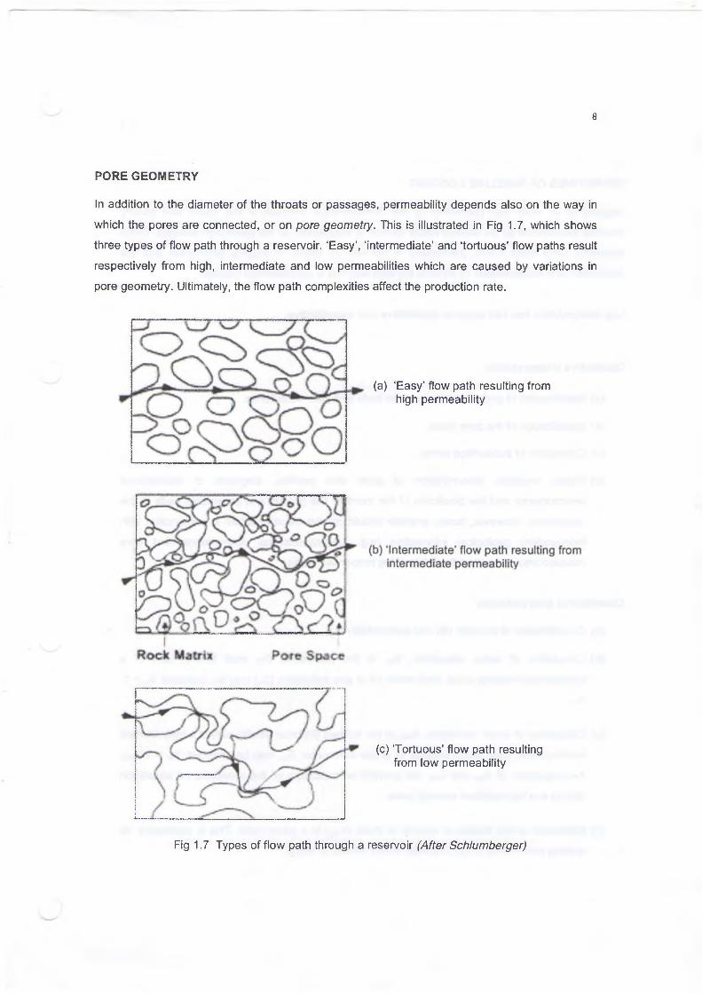
PORE GEOMETRY

In addition to the diameter of the throats or passages, permeability depends also on the way in

which the pores are connected, or on pore geometry. This is illustrated in Fig 1.7, which shows

three types of flow path through a reservoir. ‘Easy’, ‘intermediate’ and ‘tortuous’ flow paths result

respectively from high, intermediate and low permeabilities which are caused by variations in

pore geometry. Ultimately, the flow path complexities affect the production rate.

(a) ‘Easy’ flow path resulting from high permeability

(c) ‘Tortuous’ flow path resulting from low permeability

Fig 1.7 Types of flow path through a reservoir (After Schlumberger)

OBJECTIVES OF WIRELINE LOGGING

Logging of oil wells was pioneered by the Schlumberger brothers in the 1920s and quickly

became established as an indispensable source of information in the petroleum industry. Great

advances have been made, particularly in the last 25 years, in logging techniques and the

acquisition and interpretation of wireline log data are now a sophisticated science.

Log interpretation has two aspects: qualitative and quantitative.

Qualitative Interpretation

(a) Identification of porous and permeable beds and their boundaries.}

(b) Identification of the pore fluids.

(c) Correlation of subsurface strata.

(d) Facies analysis: determination of grain size profiles, diagnosis of depositional

environments and the prediction of the trend of the porous and permeable beds in the

subsurface. However, facies analysis should always be undertaken in conjunction with

independent geological information (e.g. sedimentological observations and core

descriptions) and not on the basis of log responses alone.

Quantitative Interpretation

(a) Quantification of porosity (Ф) and permeability (k).

(b) Calculation of water saturation, Sw, in the uninvaded (by mud filtrate) part of a

hydrocarbon bearing zone, from which oil or gas saturation (Sh) may be deduced: Sh - 1*

Sw-

(c) Calculation of water saturation, Sxo, in the flushed (by mud filtrate) part of a hydrocarbon

bearing zone, from which residual oil or gas saturation, Sor, may be deduced: Sor = 1-Sxo-

A comparison of Sw and Sx0 will provide an indication of the moveable oil saturation

(MOS) in a hydrocarbon bearing zone.

(d) Estimation of the fractional volume of shale (VSh) in a given zone. This is necessary for

making corrections to log readings for the effects of shale.

THE BOREHOLE ENVIRONMENT: INVASION EFFECTS

Invasion is the result of the rotary drilling process which involves the pumping of a fluid (usually

a water- or an oil-based mud) down the inside of the drill pipe and returns to the surface through

the annular space between the drill pipe and the sides of the borehole (Figure 1.8). Invasion

affects only the porous and permeable zones; tight formations permit little or no invasion.

m ud

11

During drilling the mud pressure in the annulus, Pm, must be kept greater than the hydrostatic

pressure of fluid in the formation pores, Pr to prevent a blowout. The differential pressures, Pm -

Pr, which is typically a few hundred psi, forces drilling fluid into the formation. As the mud filters

into the porous layers, it displaces some of their content, replaces them with mud filtrate, and

creates a cylindrical fluid distribution pattern. At the same time, the filtration effect of the process

causes the deposition of some of the material suspended in the mud on the porous rock faces

surrounding the borehole wall. As the mud cake thickens, its low permeability causes it to form a

barrier, and eventually the flow of filtrate into the porous layers virtually ceases. The thickness of

the mud cake is generally between 1/8 in and V* in.

In the immediate vicinity от tne borehole, almost all the formation water and some of the

hydrocarbons, if present, are displaced. This is referred to as the flushed zone,, the width of

which is usually between 3 and 4in. Away from the borehole the effect of the flushing becomes

progressively less marked. The flushed zone is therefore surrounded by a transition zone

beyond which lies the uninvaded part of the porous layer (Fig 1.9). As shown in Fig 1.10,

invasion brings about a cylindrical distribution of the fluids with respect to the axis of the

borehole.

Formation water

Uninvaded zone

Mixture of mud filtrate and formation water

Transition zone Ш~ 1

Oil

Mud filtrate

Water

Flushed Zone

Fig 1.9 Invasion effects in a permeable zone (Schlumberger)

IN V A D E D ZO NE

o rig in a l d r il l in g mudfo rm a tio n flu id s f i l t r a te

d e p th o f in va s io n

d ia m e te r o f in va s io n

Fig 1.10 Invasion produces a cylindrical distribution of thedisplaced fluids around the well (After Rider, 1996)

Factors that determine the depth of invasion include the type of mud, the differential pressure

between the mud in the borehole and the formation, and the porosity and permeability of the

formation. The most important of these factors, however, are porosity and permeability. Once

the mud cake builds up, due to its low permeability relative to that of the average formation,

almost all of the pressure differential ( P m-P r ) is across the mud cake and little is applied to the

formation. Consequently, in a given time the same volume of fluid will invade different

formations, regardless of their porosities or permeabilities (unless permeability is below about

1.0 md). This means the depth of invasion will be minimum at high porosity where large storage

space is available to accommodate the invading fluid and maximum at low porosity where little

room is available. It is approximately proportional to Other factors being constant, invasion

depth will double as porosity decreases from 36% to 9%, for example.

MATRIX CONCEPT

To a geologist the term 'matrix' refers to the fine-grained material that occurs between sediment

grains and tends to inhibit porosity and permeability. In wireline log interpretation, by contrast,

the term 'matrix' has an entirely different connotation; it refers to the actual mineral grains that

comprise the bulk of a sedimentary rock (Fig 1.11). Certain matrix properties of rocks such as

grain density (pma) and grain acoustic interval transit time (tma) must be considered in the

interpretation of some types of logs. In non-porous rocks bulk density (pb) and interval transit

time (t) measurements approach the values associated with pure minerals (i.e. all matrix, no

porosity).

sense

Fig 1.10 Geological and Petrophysical definitions of matrix

rt cCO ^ п ч е Н olo. ViMsO ,DATA ACQUISITION

A variety of methods are used in the acquisition of log data.

Conventional wireline (WL) logging involves lowering a special instrument down the well. The

instrument is attached to a calibrated cable which also carries the power supply to the tool. It is

lowered into the well and then pulled up, providing a continuous record of the rock

characteristics that the device is designed to detect. To minimise costs, a number of logs are

recorded simultaneously. A logging string is typically 3 5/8in in diameter and 25 to 60ft long,

consisting of several different tools as shown in Fig 1.12. Logging speed range is between 1,800

and 5,400ft/hr and is kept constant during individual surveys. The most commonly used is

MatrixPetrophysical

MatrixGeological sense

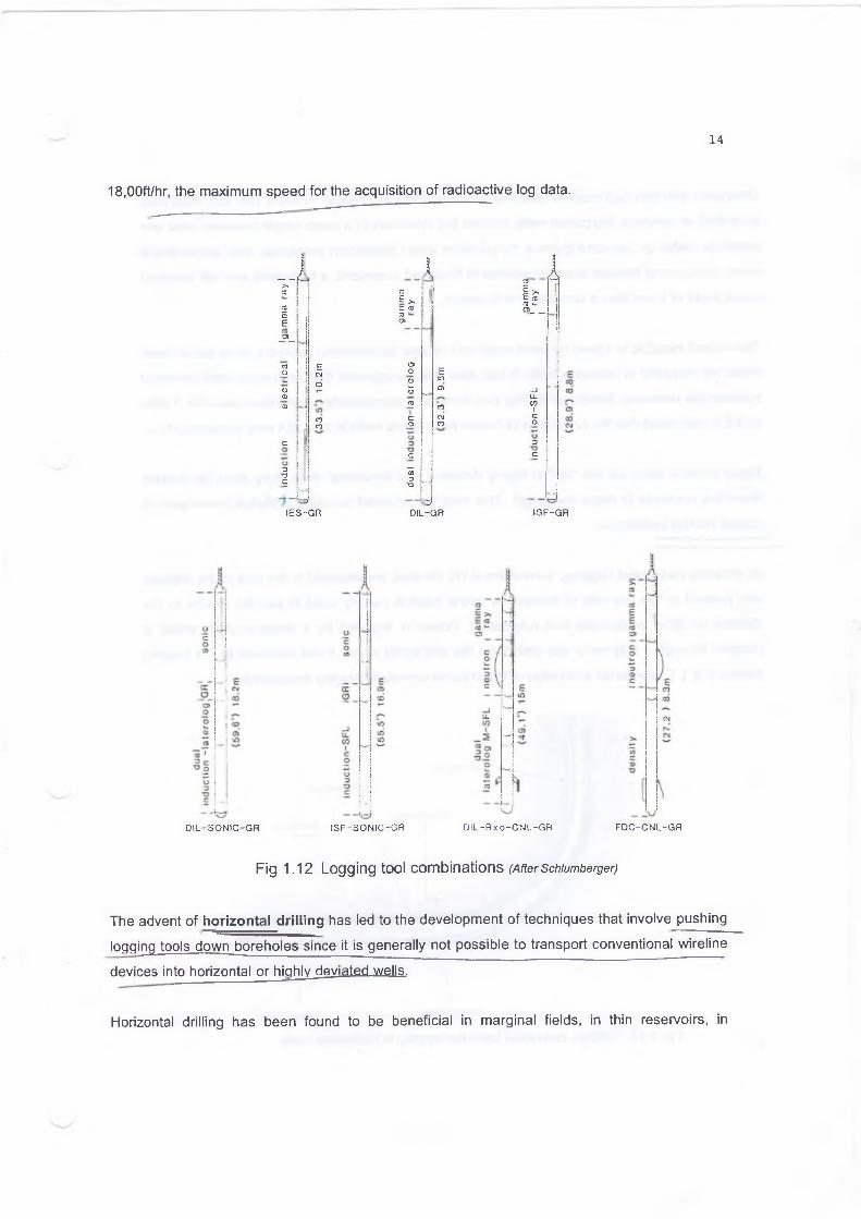
18,00ft/hr, the maximum speed for the acquisition of radioactive log data.

- J1

А>403

CO

сзЕ >,С V3

а}

1 *«= cs<3 v_Oi__£

e_p_

сэа>

яо Е

: 04а>о Е

сооо<SJ

| о

1

о5 _ J2

а>

со

_Jll-со1

! со ! со

с_о

CJсо

со

с 1 3;

с с

3ГУс

"3э•О “

У УIES-G R DIL-GR ISF-G R

D ll-S O N IC -G R IS F -S O N IC -G R D IL -R x o -C N l-G R FD C -C N L-G R

Fig 1.12 Logging tool combinations (After Schlumberger)

The advent of horizontal drilling has led to the development of techniques that involve pushing

logging tools down boreholes since it is generally not possible to transport conventional wireline

devices into horizontal or highly deviated wells.

Horizontal drilling has been found to be beneficial in marginal fields, in thin reservoirs, in

reservoirs with thin hydrocarbon columns or in fractured pay zones. In fields with thin reservoirs

or limited oil columns, horizontal wells expose the drainhole to a much larger reservoir area and

minimise water or gas coning since they induce lower drawdown pressures than conventional

wells. Since most fissures are near vertical in fractured reservoirs, a horizontal well will intersect

many more of them than a conventional borehole.

The overall result is to speed up production and reduce hydrocarbon recovery costs since fewer

wells are required to sweep a field. It has also been suggested that horizontal wells increase

recoverable reserves. Horizontal drilling has increased progressively worldwide since the 1990s

and it is estimated that the proportion of horizontally drilled wells in the USA now exceeds 50%.

Since wireline tools will not "fall" in highly deviated and horizontal wells, they must be pushed

down the borehole to reach the target. This may be achieved by using drillpipe conveyed or

coiled tubing techniques.

In drillpipe conveyed logging, conventional WL devices are attached to the end of the drillpipe

and pushed to the intervals of interest. A swivel head is usually used to join the device to the

drillpipe to allow preferential tool orientation. Power is supplied by a wireline cable which is

pumped through a side entry sub and down the drill string where it wet connects to the logging

device. Fig 1.13 shows an illustration of the drillpipe conveyed logging arrangement.

Fig 1.13 Drillpipe conveyed tools for logging in horizontal wells

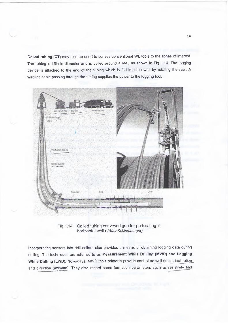
Coiled tubing (CT) may also be used to convey conventional WL tools to the zones of interest.

The tubing is l.5in in diameter and is coiled around a reel, as shown in Fig 1.14. The logging

device is attached to the end of the tubing which is fed into the well by rotating the reel. A

wireline cable passing through the tubing supplies the power to the logging tool.

Fig 1.14 Coiled tubing conveyed gun for perforating in horizontal wells (After Schtumberger)

Incorporating sensors into drill collars also provides a means of obtaining logging data during

drilling. The techniques are referred to as Measurement While Drilling (MWD) and Logging

While Drilling (LWD). Nowadays, MWD tools primarily provide control on well depth, inclination

and direction (azimuth). They also record some formation parameters such as resistivity and

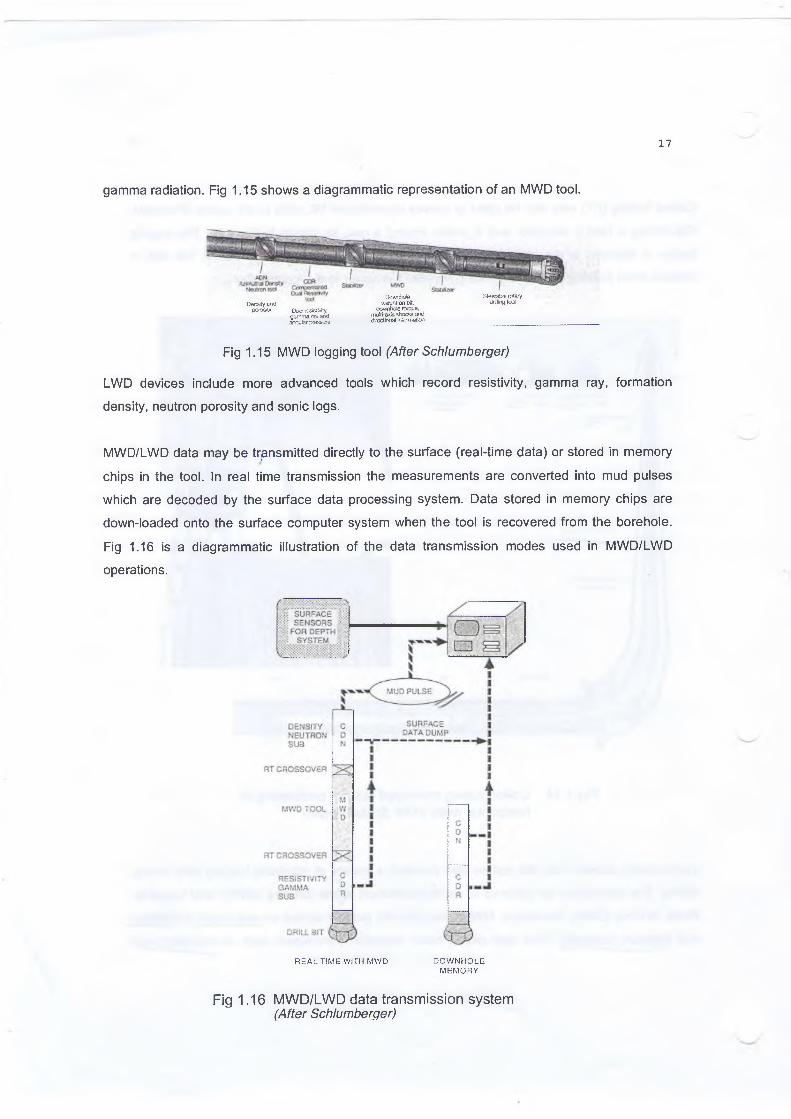
gamma radiation. Fig 1.15 shows a diagrammatic representation of an MWD tool.

Oownhcie weight on bit,

ctowrfioie torque, multi-axis shocks and directional information

Steerabie rotary drilling tedDensity and

porosrty Dua: resistivity: gamma ray and annular pressure

Fig 1.15 MWD logging tool (After Schlumberger)

LWD devices include more advanced tools which record resistivity, gamma ray, formation

density, neutron porosity and sonic logs.

MWD/LWD data may be transmitted directly to the surface (real-time data) or stored in memory

chips in the tool. In real time transmission the measurements are converted into mud pulses

which are decoded by the surface data processing system. Data stored in memory chips are

down-loaded onto the surface computer system when the tool is recovered from the borehole.

Fig 1.16 is a diagrammatic illustration of the data transmission modes used in MWD/LWD

operations.

REAL TIME WITH MWD DOWNHOLEMEMORY

Fig 1.16 MWD/LWD data transmission system (After Schlumberger)

/ Advantages of MWD/LWD include:

V (a) Savings in rig time.

(b) Current LWD measurements provide resistivity, gamma ray, neutron, density, sonic and

formation image logs as well as pore pressure.

(c) Provision of real time data helping in optimising drilling operations—early detection of

pore pressure changes that require mud weight adjustment, selection of casing and

coring points and continuous directional information; and

(d) "Insurance” logs in case of loss of hole.

Future developments include the introduction of tools measuring microresistivity.

Figure 1.17 provides a comparison between LWD and WL logs. The recording shows that MWD

logging results compare reasonably well with those obtained by WL measurements.

NEUTRON RE5ISTJVFTT

UIRSLJME NPH1 / f t ; 3

-0.15 0.*4 U fR ElIW - ILO lLu /Я»3

F -0 200. С

ffclO CN0/R;.' j

-1S.0 «5 .С

?.o

WIRELINE - iL f!

200. С

ti

ГГнО EWR/fi;i

coo .a

<

,J i

Z 5 *

<

1 i j

I | i :

1 l ! i

£! i 1 j | j

j

г

Щ%

i;

i;

— T r^ t l t

.!

| |

i |

Fig 1.17 Comparison of WL and LWD logs (After Schlumberger)

Nowadays, LWD is used in the drilling of most production and infill wells.

LOG DATA RECORDING FORMAT

Traditionally, the various measurements are presented graphically alongside a depth-scale. In

the petroleum industry, the API (American Petroleum Institute) grid is the standard log data

recording format. The total width of the log grid is 8.25in, and it is divided into three curve tracks

and a narrow column for recording the depth.

Track one is to the left of the depth column, and tracks two and three are to its right. Each track

is 2.5in wide, while the width of the depth column is 0.75in. The tracks are divided or scaled, the

divisions being referred to as the grid scale.

Three types of grids are in use: linear, logarithmic and split (Fig 1.18). Track one is always linear

while tracks two and three may be linear, logarithmic or split, depending on the data recorded.

The linear grid begins at zero while the logarithmic scale starts at 0.2 and covers a much greater

range of values. It is used for recording parameters that show large variations such as resistivity,

a common scale range being 0.2 ohm-m to 2000 ohm-m.

Fig 1.18 The three common log grids (After We I ex)

DIGITAL LOGS

Nowadays log data are recorded digitally. Digital recording is not a new phenomenon and digital

logs have been available since the 1960s. Their use, however, dates from the 1980s with the

application of computers to the evaluation of log data through the development of interpretation

programmes and their rapid proliferation in the industry. A large variety of interpretation software

is now available commercially from the major service companies (Schlumberger, Baker Atlas

and Haliburton) and specialist consultancies and many operators have developed their own in

house interpretation programmes.

Log data recordings on CD-Roms have been available since 1985 but did not gain favour in the

industry due to security problems.

The advent of workstation based interpretation further expanded the use of digital logs.

Worksations allow the integration of geophysical and log data in the interpretation of seismic

sections.

TYPES OF LOGS

A large variety of wireline logs is currently in use. Acquisition of some requires an open hole

(uncased) and the presence of a conductive mud, while others may be run in wells containing

non-conductive drilling fluids (such as an oil-based mud, gas or air), or even in cased wells.

As mentioned above, this course is concerned with the acquisition and interpretation of open

hole logs, and these may be conveniently classified as follows:

1. Electric logs.

2. Acoustic or sonic log.

3. Radioactive or nuclear logs.

4. Electromagnetic Propagation Tool (EPT).

5. Nuclear Magnetic Resonance log (NMR).

6. Dipmeter and formation image logs

NOMENCLATURE

The subject lends itself well to the use of abbreviations and symbols. A large number of these,

referring to the various properties of the formations penetrated by the well, borehole parameters

and the measurements made in logging, is in use. The most commonly used abbreviations and

symbols are listed in Tables 1.1-1.7 (Schlumberger).

TABLE 1.1 FORMATION CHARACTERISTICS, DRILLING MUD AND BOREHOLE PARAMETERS

a Tortuosity factor Ф Porosity

BHT Bottom Hole Temperature Фа Absolute porosity

BS Bit size Ф е

(PHIE) Effective porosity

BVW Bulk Volume Water SPI Secondary Porosity Index

CALI Caliper MOS Moveable Oil Saturation(Sxo ■ Sw)

dh Diameter of borehole m Cementation factor

d. Diameter of flushed zone n Saturation exponent

dj Diameter of invaded zone ROS Residual Oil Saturation (1.0-Sxo)

EFT Estimated Formation Temperature s h Hydrocarbon saturation (1.0-Sw)

F Formation Factor Sw Water saturation of uninvaded zone

hmc Thickness of mudcake Swi Irreducible water saturation

к Permeability SxoWater saturation of flushed zone

kA Absolute permeability Sw/Sxo Moveable hydrocarbon index

kE Effective permeability T Formation temperature

kr Relative permeability VshFractional volume of shale in formation

TABLE 1.2 ELECTRIC LOGS

AIT Array Induction Tool PL Proximity Log

CHFRCased Hole Formation Resistivity Tool

R Resistivity

DIL Dual Induction Laterolog Rilm Resistivity Induction Log Medium

DLL Dual Laterolog R|_Ld Resistivity of Laterolog Deep

HRLA High Resolution Laterolog Array Rlls Resistivity of Laterolog Shallow

IDPH Induction Deep Phasor RLL8 Resistivity of Laterolog 8

IL Induction Log Rm Resistivity of drilling mud

ILD Deep Induction Log Rmc Resistivity of mudcake

ILM Medium Induction Log Rmf Resistivity of mud filtrate

IMPH Induction Medium Phasor Rmll Resistivity of Microlaterolog

LL Laterolog Rmsfl Resistivity of MicroSpherically Focused Log

LLD Deep Laterolog Ro Resistivity of 100% water saturated formation (‘wet resistivity’)

LLS Shallow Laterolog Rs Resistivity of adjacent beds

LL8 Laterolog 8 R, Resistivity of uninvaded zone

LN Long (64” ) Normal Rw Resistivity of formation water

MINV Micro Inverse curve Rxo Resistivity of flushed zone

ML Microlog SN Short (16") Normal

MLL Microlaterolog SP Spontaneous Potential

MNOR Micro Normal curve PSP Pseudostatic Spontaneous Potential

MSFL MicroSpherically Focused Log SSP Static Spontaneous Potential

TABLE 1.3 ACOUSTIC (SONIC) LOG

AST Array Sonic Toolt (At; Dt)

Interval transit time of formation

Bcp Acoustic porosity compaction factor tf Interval transit time of fluid in formation

вне Borehole Compensated Sonic Log tma Interval transit time of formation matrix

LSS Long Spacing Sonic Log

TABLE 1.4 RADIOACTIVE LOGS

CGR Computed Gamma Ray P e ( P E F ) Photoelectric absorption factorCNL/CNT Compensated Neutron Log/Tool pb (RHOB) Bulk density of the formationFDC Formation Density Compensated

Log Pf Density of fluid in formation

GR Gamma Ray Log Ph Hydrocarbon densityG Rclaen Gamma Ray reading from clean

zone Pma Density of the formation matrix

GRshale Gamma Ray reading from shale SGR Standard Gamma RayG Rzone Gamma Ray reading from

formationSNP Sidewall Neutron Porosity

GST Gamma Ray Spectrometry Tool TDT Thermal Decay Time LogLDT Litho-Density Tool TNPH Total Neutron Porosity

NGS Natural Gamma Ray Spectrometry Log U Volumetric photoelectric

absorption indexNPHI Neutron porosity

ATBLE 1.5 ELCTROMAGNETIC PROPAGATION TOOL (EPT)

EATT Electromagnetice signal attenuation ratetpl EPT travel time of formationtpm a EPT travel time of matrixtpo EPT travel time of a low attenuation (lossless) mediumtpw EPT travel time of water

TABLE 1.6 NUCLEAR MAGNETIC RESONACE LOG (NMR)

ADEPT Adaptable Electromagnetic Propagation ToolCMR Combinable Magnetic Resonance ToolEATT Electromagnetic Wave AttenuationFFI Free Fluid IndexMRIL Magnetic Resonance Imaging Log

TABLE 1.7 PLATFORM EXPRESS

AIT Array Induction Imager ToolHALS High Resolution Azimuthal Laterolog SondeHGNS Highly Integrated Gamma Ray Neutron SondeHLLD High Resolution Deep LaterologHRMS High Resolution Mechanical SondeMCFL Micro-Cylindrically Focused LogTLD Three Detector Lithology Density Tool

2. ELECTRIC LOGS

INTRODUCTION

Methods of measuring the electrical properties of rocks penetrated by boreholes were the first to

be developed and used in the petroleum industry. The instrument used consists of a system of

electrodes attached to a cable which carries also the electric current. The acquisition of most of

the electric logs requires an open or uncased well containing a water-based, conductive drilling

fluid. Only the electric induction log can be run in the presence of a non-conductive drilling fluid

such as an oil-based mud (see below). Drilling with non-conductive fluids, therefore, limits the

choice of the electric logs that can be run.

Electric logs fall into two main categories: the spontaneous potential (SP) which measures a

naturally occurring phenomenon, and the resistivity devices which record the resistance offered

by the rocks surrounding the borehole to the passage of an electric current.

THE SP LOG

The SP curve is a recording versus depth of the difference in electric potential between a fixed

electrode at the surface and a moving electrode in the borehole. It is measured in millivolts, and

there is no absolute zero; only changes in potential are recorded. It is recorded on track 1, and is

always linear. The SP log has the following applications:

(a) Identification of permeable beds and the location of their boundaries.

(b) Determination of the formation water resistivity in the uninvaded zone (Rw).

(c) Estimation of the degree of shaliness of reservoir rocks.

Two types of potential may contribute to the SP effect. These are the electrochemical (Ec) and

the electrokinetic (Ek) potentials. The latter, also known as the electrofiltration or streaming

potential, is in most cases negligible, and in log analysis the observed SP response is assumed

to be solely due to the electrochemical component. The origins of these potentials are discussed

briefly below.

Ek

In general, an Ek is produced by the flow of an electrolyte through a porous, non-metallic

medium. In the case of the SP response, the Ek results from the movement of filtrate through the

mud cake that builds up on a porous and permeable formation. Its magnitude is influenced by a

number of factors, the most important of which are the differential pressure producing the flow

and the resistivity of the formation water (Rw)- During the initial stages of mud cake formation Ek

is significant, but as the mud cake thickens its permeability diminishes rapidly, causing it to

isolate the porous bed from the borehole. As the flow of filtrate into the porous bed virtually

ceases, all the differential pressure is expended on the mud cake, and this effectively ends the

generation of Ek. However, in cases where unusually high differential pressures prevail, Ek

effects may be substantial. Such cases result from drilling with very heavy muds, or when

low-pressure formations are penetrated. Large Ek effects may also be observed in very low

permeability (less than 5 md) formations. Low permeability results in a low rate of filtrate

invasion, and this in turn means that little or no mud cake will build up. Consequently, the

formation remains in communication with the borehole, and nearly all the differential pressure is

applied to the formation. If the formation is clean (shale-free), contains brackish water and the

drilling mud is resistive, the low permeability Ek effect may cause a large deflection in the SP

curve. Such a deflection cannot be used in quantitative interpretation, nor is it indicative that the

zone involved will produce any fluid.

Although these effects occur infrequently, the conditions that cause them are a possible source

of large Ek values.

Ec

The Ec component is the main source of the deflections in the SP curve and results from the

transfer of ions from a more concentrated electrolyte (usually the uninvaded zone formation

water) to a less concentrated electrolyte (usually the mud in the borehole) through a

semi-permeable membrane (e.g. a sand-shale contact). Sodium chloride is the main source of

ions both in the formation water and the drilling mud.

The transfer of ions constitutes an electric current, and as shown in Fig 2.1, these currents flow

through four different media, namely, the mud in the borehole, the invaded part of the porous

and permeable bed, the uninvaded part of the same and the surrounding shales. Movement of

ions takes place in two ways: (a) through the shales, above and below the porous and

permeable bed, and (b) at the boundary between the invaded and uninvaded parts of the porous

and permeable bed where two solutions of different salinities are in direct contact. The

movement of ions through the surrounding shales gives rise to a membrane potential, while the

direct transfer of ions at the invaded - uninvaded zone boundary produces a liquid

Fig 2.1 Diagrammatic representation of the membrane potential component of the SP (After Welex)

junction potential. The sum of these two independent potentials makes up the electrochemical

component of the SP phenomenon.

The membrane potential is related to the selective passage of ions through the shales above

and below the porous and permeable bed. Due to their layered structure and the charges on the

layers, shales are permeable to the Na+ cations but impervious to the СГ anions. When a shale

separates sodium chloride bearing solutions of different salinities, the Na+ cations move through

the shale from the more concentrated solution. This movement of charged ions is an electric

current, and the force causing them to move constitutes a potential across the shale. The curved

arrow in the upper half of Fig 2.2 shows the direction of current flow corresponding to passage of

Na+ ions through the adjacent shale from a more saline formation water in the bed to the less saline mud.

Fig 2.2 Diagrammatic representation of the liquid junction component of the SP (After Schlumberger)

The liquid junction potential arises from the transfer of ions across the invaded

zone/uninvaded zone interface. Here Na+ and СГ ions can transfer from either solution to the

other. Since СГ ions have a greater mobility than Na+ ions, the net result is a flow of negatively

charged particles from the more concentrated solution to the less concentrated solution. This is

equivalent to a conventional current flow in the opposite direction, indicated by the straight

arrow, A, in the upper half of Fig 2.2. The liquid-junction potential is only about one-fifth the membrane potential.

The first step in the interpretation of the SP log is the establishment of 'sand' and ’shale’ lines as

shown in Fig 2.3. These are arbitrary limits, with the former normally representing the maximum

deflection to the left, the latter representing the maximum deflection to the right. Deflections to

the left of the shale line are regarded as normal or negative, and correspond to porous and

permeable zones containing a more saline interstitial water than the drilling mud (i.e. Rw< Rmf).

In these cases the SP currents flow in the direction shown in Fig 2.4.

Fig 2.3 SP log presentation in a sand-shale sequence (After Schlumberger)

If the mud is more saline than the formation water (this could happen if the mud is very salty or

the formation water is brackish or fresh in which case Rw> R m f), the S P currents flow in the

opposite direction to that shown in Fig 2.4, and the corresponding deflection will be to the

Fig 2.4 S P response associated with a clean, permeable bed containing formation water more saline than the drilling mud filtrate (Rw < Rmf) (After Welex)

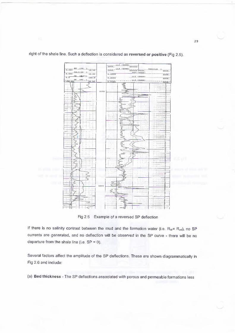
right of the shale line. Such a deflection is considered as reversed or positive (Fig 2.5).

Fig 2.5 Example of a reversed SP deflection

If there is no salinity contrast between the mud and the formation water (i.e. Rw= Rmf), no SP

currents are generated, and no deflection will be observed in the SP curve - there will be no

departure from the shale line (i.e. SP = 0).

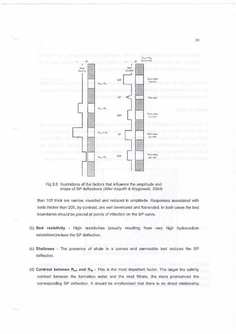
Several factors affect the amplitude of the SP deflections. These are shown diagrammatically in

Fig 2.6 and include:

(a) Bed thickness - The SP deflections associated with porous and permeable formations less

+

ShaleBaseline

+Rrf»R„

for all sands

ShaleBaseline

SSP

s p < T

PSP

SP

PSP

;

mm

Thick clean wet sand

Thick shaly wet sand

Thick clean gas sand

Thick shaly gas sand

Fig 2.6 Illustrations of the factors that influence the amplitude and shape of SP deflections (After Asquith & Krygowski, 2004)

than 10ft thick are narrow, rounded and reduced in amplitude. Responses associated with

beds thicker than 20ft, by contrast, are well developed and flat-ended. In both cases the bed

boundaries should be placed at points of inflection on the SP curve.

(b) Bed resistivity - High resistivities (usually resulting from very high hydrocarbon

saturations)reduce the SP deflection.

(c) Shaliness - The presence of shale in a porous and permeable bed reduces the SP

deflection.

(d) Contrast between Rmf and Rw - This is the most important factor. The larger the salinity

contrast between the formation water and the mud filtrate, the more pronounced the

corresponding SP deflection. It should be emphasised that there is no direct relationship

between the value of permeability and the amplitude of the SP deflection, nor does the

deflection bear any direct relation to porosity; a high porosity and permeability zone is not

necessarily associated with a high amplitude SP response.I

In summary, the SP log qualitatively distinguishes between permeable and impervious beds,

and provides information on the salinity of the formation water relative to that of the drilling mud.

The quantitative application of the SP curve will be discussed later.

STATIC SP (SSP)

As stated above, the amplitude of the SP deflection associated with thin beds is reduced. The

full SP, or the SSP, is developed only in thick, clean (shale-free) and water bearing zones in

which Rmf - Rw. The minilmum bed thickness required for the development of the SSP is about

20ft. In thin beds a correction must be applied to the SP reading in order to obtain the SSP. This

is done by reference to charts provided by the various service companies. One such chart is

presented in Fig 2.7. All these charts are entered by plotting Ri/Rm against bed thickness, and

Fig 2.7 SP bed thickness correction (After Baker Atlas)

reading the correction factor on the x-axis. It should be noted that Rm must be at formation

temperature. This value of Rm is obtained by converting mud resistivity at surface temperature

(measured and recorded on the log heading by the service company engineer) to its

corresponding value at formation temperature.

Knowledge of the SSP is essential for the derivation of Rw which in turn is required for the

calculation of water saturation in the uninvaded zone. There is an equation which relates the

SSP to the conductivities of the mud filtrate (cmt) and the formation water (cw):

2.1 vSSP — К log (cw/Cmf)i 2.

where К is a constant, the value of which is dependent on the formation temperature. Usually,

К = 61 + 0.133 T(°F) or К = 65 + 0.24T (°C).

In practice, however, cmf and cw are of little value, as they cannot be readily quantified. It would

therefore be more useful to express these in terms of measurable quantities, namely, Rw and

Rmf. For pure sodium chloride solutions that are not too concentrated, resistivities are inversely

proportional to chemical activities (Fig 2.8), and equation 2.1 may therefore be written as:

SSP = - К log (R m f/R w ) 2.2

N a + Activity (Gr-lon/Liter, Total Na)

Fig 2.8 Na+ NaCI Resistivity relationship (After Schlumberger)

However, as shown in Fig 2.8, resistivity and chemical activity are no longer linearly related in

solutions containing more than 0.7 gm-ions/litre of Na+. Consequently, R mf and R w must be

converted to values that are linearly related to their respective chemical activities. These values

are referred to as equivalent resistivities, and are denoted by R we and R mfe- Thus the standard

equation that relates the SSP to the mud filtrate and uninvaded formation water resistivities is:

SSP = - К log (R m fe /R w e) 2.3

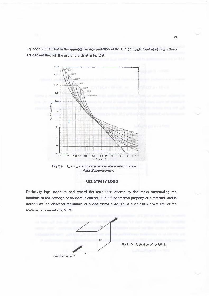
Equation 2.3 is used in the quantitative interpretation of the SP log. Equivalent resistivity values

are derived through the use of the chart in Fig 2.9.

0.001

0.002

0.005

0.01

0.02

fs3J 0.05

CC о2CC 0.1

0.2

0.5

1.0

2.00.005 0.01 0.02 0.03 0.05 0.1 0.2 0.3 0.5 1.0 2 3 4 5

R„ or Я,* (ohm-m)

Fig 2.9 Rw" Rwe" formation temperature relationships (After Schlumberger)

RESISTIVITY LOGS

Resistivity logs measure and record the resistance offered by the rocks surrounding the

borehole to the passage of an electric current. It is a fundamental property of a material, and is

defined as the electrical resistance of a one metre cube (i.e. a cube 1m x 1m x 1m) of the

material concerned (Fig 2.10).

Fig 2.10 Illustration of resistivity

1mElectric current

Resistivity (R) is the reciprocal of conductivity (c):

R = 1/c 2.4

Resistivity is related to electrical resistance by the following equation:

R = rA/L 2.5

r = resistance in ohms (Q)

A = cross-sectional area of the conducting medium (m2)

L = length of the conducting medium (m)

Substituting for Q resistance, m2 for A, and m for L in equation 2.5:

R = £2m2/m 2.6

Resistivity is therefore expressed in ohms m2/m or ohm.m.

In sedimentary rocks the ability to conduct is related to the movement of ions present in the

formation water; clean, dry reservoir rocks and hydrocarbons are insulators, characterised by

low conductivity and therefore high resistivity. Consequently, the only part of a formation which

conducts electricity is the interstitial water. The resistivity of the water depends on the quantity of

dissolved salts present (mostly NaCI); the more saline the formation water, the higher its

conductivity and the lower its resistivity. Temperature is another important factor. Ionic activity

increases with increasing temperature, lowering resistivity.

In summary, the factors influencing the resistivity of a clean (shale-free) rock are:

1. Formation water resistivity (Rw)

2. Temperature

3. Presence of hydrocarbons

4. Magnitude of porosity (Ф).

The influence of porosity is due to the fact that conductivity depends on the number of ions

available in a solution to carry the electric charge; other factors being equal, the higher the

number of ions, the greater the conductivity. The number of ions depends on water-filled

connected porosity; therefore, the higher the porosity, the greater the number of available ions

and the higher the conductivity.

INVASION AND RESISTIVITY PROFILES

As already discussed, all porous and permeable beds penetrated by a borehole become

invaded by mud filtrate. The invaded formation consists of a flushed zone, close to the borehole,

surrounded by a transition zone which in turn is surrounded by the uninvaded or undisturbed

part of the porous and permeable bed where the original formation fluids remain uncontaminated

by the mud filtrate. The detailed distribution of these zones and the associated resistivities and

saturations are shown in Fig 2.11, and the various parameters shown were defined in Tables 1.1

and 1.2. Depth of invasion is a function of porosity and permeability, as discussed above.

t(~~j Resistivity of the zone О Resistivity of the water in the zone Д Water saturation in the zone

(Invasion diameters)

Adjacent bed

Adjacent bed

dj/dj = 2 indicates high Ф and к d/di = 5 indicates intermediate Ф d/dp Ю indicates low Ф and к

Fig 2.11 Distribution of resistivity and saturation in an invaded formation (After Schlumberger)

If the porous and permeable zone contains oil, the fraction of the original oil saturation displaced

from the flushed zone by mud filtrate invasion is represented by the difference between water

saturations in the flushed and the uninvaded zones (i.e. Sxo - Sw)- Usually, between 70% and

95% of the oil is flushed out; the remaining fraction is called residual oil, and its saturation, Sor,

equals 1 - SXo- In the uninvaded zone the original hydrocarbon saturation, Sh, remains intact,

and is given by the following equation:

Sh = 1 - Sw 2.7

Determination of Sh is one of the main objects of quantitative log interpretation.

It should be clear from the above discussion that the invasion of a porous and permeable bed

creates zones, radially distributed with respect to the borehole axis, containing different fluids

with different resistivities. This distribution of resistivity gives rise to resistivity profiles which

represent cross-sectional views of the invaded formation. There are three commonly recognized

invasion profiles: (a) step, (b) transition, and (c) annulus. These three invasion profiles are

illustrated in Figure 2.12.

STEP PROFILE

^borehole wall

* Distance from the borehole

TRANSITION PROFILE

borehole wall

ANNULUS PROFILE

borehole wall

I D istance from the borehole

R0: Resistivity of the zone 100% saturated with formation water of resistivity R w- R o is also called ‘wet resistivity’

Fig 2.12 Resistivity profiles (After Asquith & Krygowski, 2004)

The step profile has a cylindrical geometry with an invasion diameter equal to dj. Shallow

reading, resistivity logging tools read the resistivity of the invaded zone (R), while deeper

reading, resistivity logging tools read true resistivity of the uninvaded zone (Rt).

The transition profile also has a cylindrical geometry with two invasion diameters: d. (flushed

zone) and d. (transition zone). It is probably a more realistic model for true borehole conditions

than the step profile. Three resistivity devices are needed to measure a transitional profile; these

three devices measure resistivities of the flushed, transition, and uninvaded zones, Rxo, Ri, and

Rt respectively (Fig 2.12). By using these three resistivity measurements, the deep reading

resistivity tool can be corrected to a more accurate value of true resistivity, Rt, and the depth of

invasion can be determined.

An annulus profile is only sometimes recorded on a log because it rapidly dissipates with time

and can be detected only by logging soon after a well is drilled. However, it is very important as

the profile can occur only in zones which bear hydrocarbons. As the mud filtrate invades the

hydrocarbon-bearing zone, hydrocarbons move out first. Next, formation water is pushed out in

front of the mud filtrate forming an annular (circular) ring at the edge of the invaded zone (Fig

2.12). The annulus effect is characterised by a higher Rt reading than a simultaneously recorded

Ri measurement.

)

Resistivity profiles are developed when three resistivity curves (Rxo, Ri and Rt) are recorded

/simultaneously. They are useful aids in quick-look qualitative interpretation; together with an SP

curve, the resistivity responses are used to (1) identify porous and permeable formations, and

(2) detect hydrocarbon-bearing zones. Because of their importance, resistivity profiles for both

water-bearing and hydrocarbon-bearing zones are discussed here. These profiles vary,

depending on the relative values of Rwand Rmf.

Water-bearing Zones

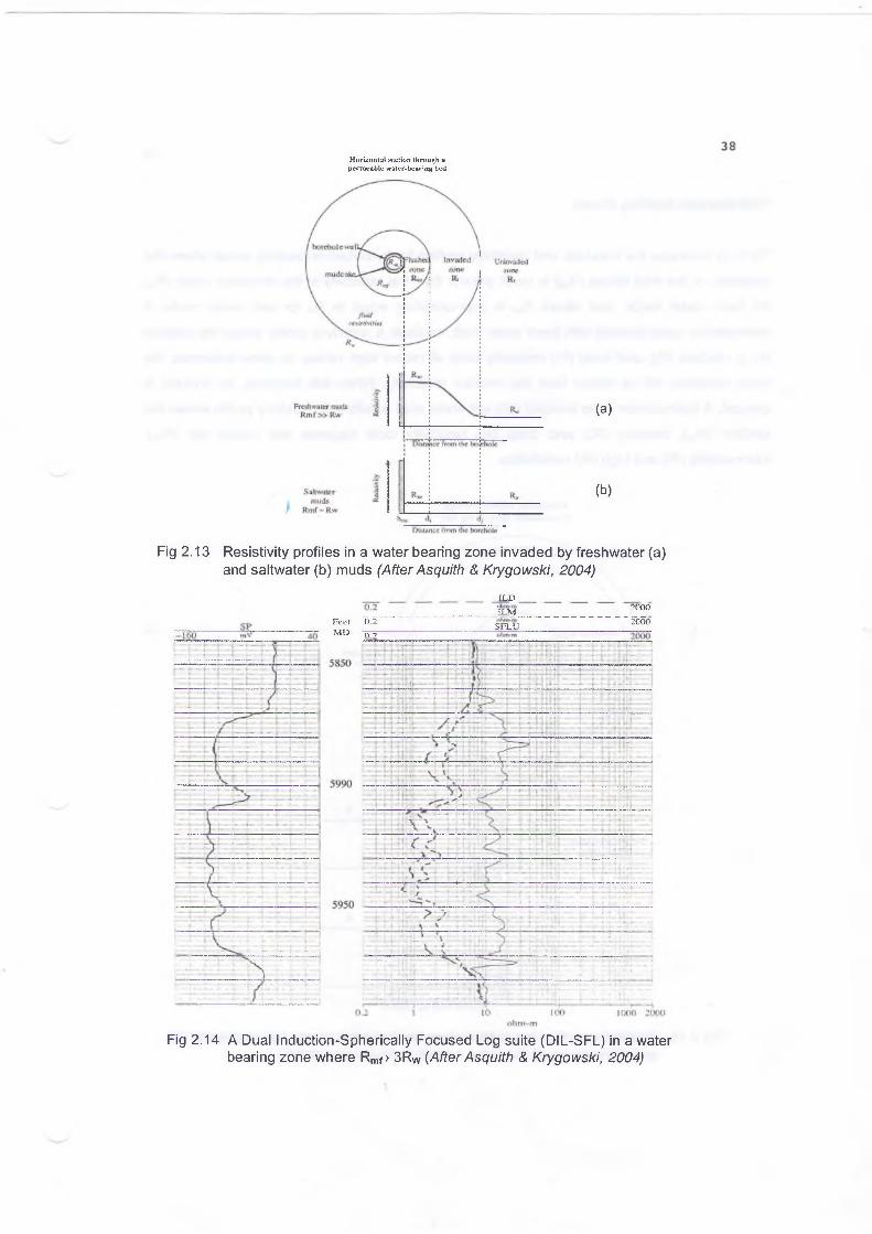
Fig 2 .1 3 illustrates the borehole and resistivity profiles for water-bearing zones where the

resistivity of the mud filtrate ( R mf) is much greater than the resistivity of the formation water ( R w)

in fresh water muds, where resistivity of the mud filtrate ( R mf) is approximately equal to the

resistivity of the formation water ( R w) in salt water muds and where the mud filtrate resistivity

( R mf) is less than that of the formation water ( R w). A fresh water mud (i.e. R mf > 3 R W) results in a

'wet' log profile where the shallow ( R xo), medium (R ,) , and deep ( R t ) resistivity tools separate and

record high ( R xo), intermediate (R j) , and low ( R t. ) resistivities. A salt water mud (i.e. R w - R mf)

results in a wet profile where the shallow ( R xo), medium (R ,) and deep ( R t) resistivity tools all

read low resistivity. Fig 2 .1 4 illustrates the resistivity curves for wet zones invaded with a fresh

water mud.

H orizon ta l .section through a perm eable water-bearing bed

(a)

(b)

Fig 2.13 Resistivity profiles in a water bearing zone invaded by freshwater (a) and saltwater (b) muds (After Asquith & Krygowski, 2004)

Feet 0 .2 M D 7Гт~

1LPjLM _

SFLU

2000

"2000

Fig 2.14 A Dual Induction-Spherically Focused Log suite (DIL-SFL) in a water bearing zone where Rmf > 3RW (After Asquith & Krygowski, 2004)

Hydrocarbon-bearing Zones

Fig 2.15 illustrates the borehole and resistivity profiles for hydrocarbon-bearing zones where the

resistivity of the mud filtrate (Rmf) is much greater than the resistivity of the formation water (Rw)

for fresh water muds, and where Rmf is approximately equal to Rw for salt water muds. A

hydrocarbon zone invaded with fresh water mud results in a resistivity profile where the shallow

(Rxo), medium (R), and deep (Rt) resistivity tools all record high values. In some instances, the

deep resistivity will be higher than the medium resistivity. When this happens, an annulus is

present. A hydrocarbon zone invaded with salt water mud results in a resistivity profile where the

shallow (Rx0), medium (RJ, and deep (Rt) resistivity tools separate and record low (Rx0),

intermediate (Ri) and high (Rt) resistivities.

Horizontal section through a permeable oil-bearing bed

Fig 2.15 Resistivity profiles in a hydrocarbon bearing zone invaded by freshwater (a) and saltwater muds (b) {After Asquith & Krygowski, 2004)

Fig 2.16 illustrates the resistivity curves for hydrocarbon zones invaded with fresh water mud.

SP-1 о 3 < 4-*- O

!--Pf ct=

r

—1-

r~t-

V-'h

r -=t- 1--- -H

—' X——

“ 1~~

1-

0.2

Feet 0,2 MD 0.2

8700

8800

JLP.ohm-m

JLM _ohm-m

SFLUohm-m

I£

SuL8

a i

2000'

'2000

2000

Fig 2.16 A Dual Induction-Spherically Focused Log suite (DIL-SFL) in a hydrocarbon bearing zone where Rmf> 3RW {After Asquith & Krygowski, 2004)

In conclusion, it is emphasised once more that invasion and the associated resistivity profiles

are unique to porous and permeable zones. Impervious formations remain uninvaded, and do

not therefore exhibit resistivity profiles. All three resistivity curves read approximately the same

value opposite an impervious bed.

RESISTIVITY MEASUREMENT

Resistivity devices are designed to measure Rxo, Ri and Rt, resistivities of the flushed (1-6in),

transition (0.5-3ft) and uninvaded (3+ft) zones respectively.

All deep and shallow/medium logs are obtained with electrodes or coils mounted on cylindrical

tools that are run more or less centralized in the hole. By contrast, the flushed zone

(microresistivity) curves are obtained with pad-mounted electrodes in contact with the borehole

wall. Nowadays the three curves are obtained simultaneously on a single pass in the hole.

Resistivity logging has advanced enormously since its introduction in the late 1920s. The

resistivity logs may be divided into conventional or non-focused devices (also known as

Electrical Survey tools - abbreviated to ES tools), focused tools, and induction systems. The

conventional resistivity devices are now obsolete, but many such logs survive in oil company

archives and it is therefore necessary to describe the way in which the tools functioned.

THE CONVENTIONAL RESISTIVITY LOGS

Until about 1950, all resistivity measurements were made with simple electrode systems shown

in Fig 2.17. These measurements produced a Short Normal (SN), a Long Normal (LN), and a

Lateral curve, depending on the spacing between the current electrode (A in Fig 2.17) and

voltage measuring electrode (M in Fig 2.17) in the borehole. The electrode spacing was 16in,

64in and 18ft 8in in the SN, LN and the Lateral curves respectively. In general, the greater the

spacing between A and M the greater was the depth of investigation. In the case of the Lateral

curve, there were two voltage recording electrodes (M and N in Fig 2.18) in the borehole, and

the resistivity was measured between these and the current electrode A. In practice, the

measurement was made between A and a point O. midway between M and N. All three curves

were recorded simultaneously.

The 16in Normal recorded Ri, while the 64in Normal and the Lateral curve responded primarily

to Rt. Fig 2.19 presents a suite of conventional resistivity logs.

The conventional logs were difficult to interpret. Extensive charts were required to correct for

borehole, bed thickness, and adjacent-bed resistivity effects. In particular, the curves were

relatively inaccurate for bed thicknesses less than about 1.5 times the spacing, i.e., 28ft for the

Lateral and 8ft for the Long Normal. The Short Normal curve was the most usable, but it was

Generator

Meter

H 0 H

Spacing J

Meter

Generator

Spacing

MoJ

Fig 2.17 Normal device - schematic Fig 2.18 Lateral device - schematicdiagram (After Schlumberger) diagram (After Schlumberger)

Fig 2.19 A suite of conventional resistivity logs (After Baker Atlas)

severely affected by invasion. The basic problem with the conventional logs was that the

direction of the survey current was not controlled (Fig 2.20). It took the path of least resistance,

favouring conductive mud and conductive shoulder beds over high resistivity beds at the level of

the tool.

Fig 2.20 Schematic representation of focused and non-focused current flow from a logging tool (After Rider, 1996)

Fig 2.21 Schematic representation of focused and non-focused current flow from a microresistivity logging tool (After Schlumberger)

A non-focused microresistivity device (for measuring Rxo) was also available. Known as the

Microlog, the device consisted of three electrodes, spaced 1 in apart, mounted on a pad and

made its measurement in contact with the borehole wall (Fig 2.21). It recorded a Microinverse

(also called the 1" x 1") and a Micronormal (also referred to as the 2") curve simultaneously.

The micronormal device investigated three to four inches into the formation, measuring Rxo, and

the microinverse investigated approximately one to two inches and measured the resistivity of

the mud cake, Rmc. The detection of mud cake by the Microlog indicated that invasion had

occurred and the formation was permeable. Permeable zones showed up on the Microlog as

positive separation when the micronormal curve read higher resistivity than the microinverse

curve (Fig 2.22). Shale zones were indicated by no separation or negative separation (i.e.

micronormal = microinverse).

The Microlog did not work well in salt water-based muds. These muds cause the formation of

conductive mud cakes, and the non-focused current tended to flow between the A and M

electrodes through the mud cake rather than penetrate the more resistive formation behind the

mud cake.

As a result of these problems, the Long Normal and Lateral curves were replaced in the 1950s

by focused logs in which the path of the survey current was controlled. The focusing minimized

borehole and adjacent bed effects and provided simultaneously both deep penetration and good

bed resolution.SP

Fig 2.22 Example of a Microlog (After Asquith & Krygowsky, 2004)

FOCUSED RESISTIVITY LOGS

These devices were introduced in the 1950s and include the Laterologs. They are designed to

measure RXo, Ri and Rt in boreholes containing salt water muds, have excellent vertical

resolution (about 2ft) and their readings are little affected by the resistivities of the adjacent

beds.

Laterolog systems contain an array of electrodes to focus the survey current and force it to flow

laterally into the formations surrounding the borehole. Focusing is achieved by two bucking

electrodes that emit a current of the same polarity as the surveying electrode but are located

above and below it (Д and A’i in Fig 2.23). The focusing, or guard electrodes, prevent the

surveying current from flowing up the borehole filled with salt water mud. The effective depth of

Laterolog investigation is controlled by the extent to which the surveying current is focused.

Fig 2.23 Schematic diagram of a focused resistivity logging tool (After Schlumberger)

Deep reading Laterologs (LLD in Fig 2.24) are therefore more strongly focused than shallow

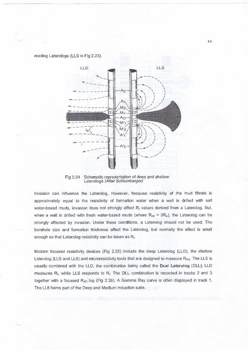
reading Laterologs (LLS in Fig 2.23).

Fig 2.24 Schematic representation of deep and shallow Laterologs (After Schlumberger)

Invasion can influence the Laterolog. However, because resistivity of the mud filtrate is

approximately equal to the resistivity of formation water when a well is drilled with salt

water-based muds, invasion does not strongly affect Rt values derived from a Laterolog. But,

when a well is drilled with fresh water-based muds (where Rmf > 3RW), the Laterolog can be

strongly affected by invasion. Under these conditions, a Laterolog should not be used. The

borehole size and formation thickness affect the Laterolog, but normally the effect is small

enough so that Laterolog resistivity can be taken as Rt.

Modern focused resistivity devices (Fig 2.25) include the deep Laterolog (LLD), the shallow

Laterolog (LLS and LL8) and microresistivity tools that are designed to measure RXo- The LLS is

usually combined with the LLD, the combination being called the Dual Laterolog (DLL); LLD

measures Rt, while LLS responds to Rj. The DLL combination is recorded in tracks 2 and 3

together with a focused RXo log (Fig 2.26). A Gamma Ray curve is often displayed in track 1.

The LL8 forms part of the Deep and Medium Induction suite.

DUAL L A T E R O L O G S

s h a l lo w d e e p

SP H E R IC A LL Y F O C U S E D TOOL

Fig 2.25 Schematic representation of the Dual Laterologs (DLL) and the Spherically focused Log (SFL)

) (After Rider, 1996)

Fig 2.26 A DLL-MSFL suite

Another R| measuring device is the Spherically Focused Log (SFL), and Fig 2.25 illustrates the

tool. It is offered as an alternative to the LL8 as part of the Deep and Medium Induction suite.

The SFL device carries nine electrodes, with the survey current emanating from the centre

electrode, A0 (Fig 2.25). Focusing electrodes enforce an approximately spherical shape on the

equipotential surface, and hence the name. The depth of penetration of the SFL is smaller than

that of the LL8. This means that the SFL gives greater weight to Rj, which is desired, but in

general it still reads too deep to give an accurate measurement of flushed zone resistivity, Rxo.

The vertical resolution of the SFL and the LL8 is about 1ft.

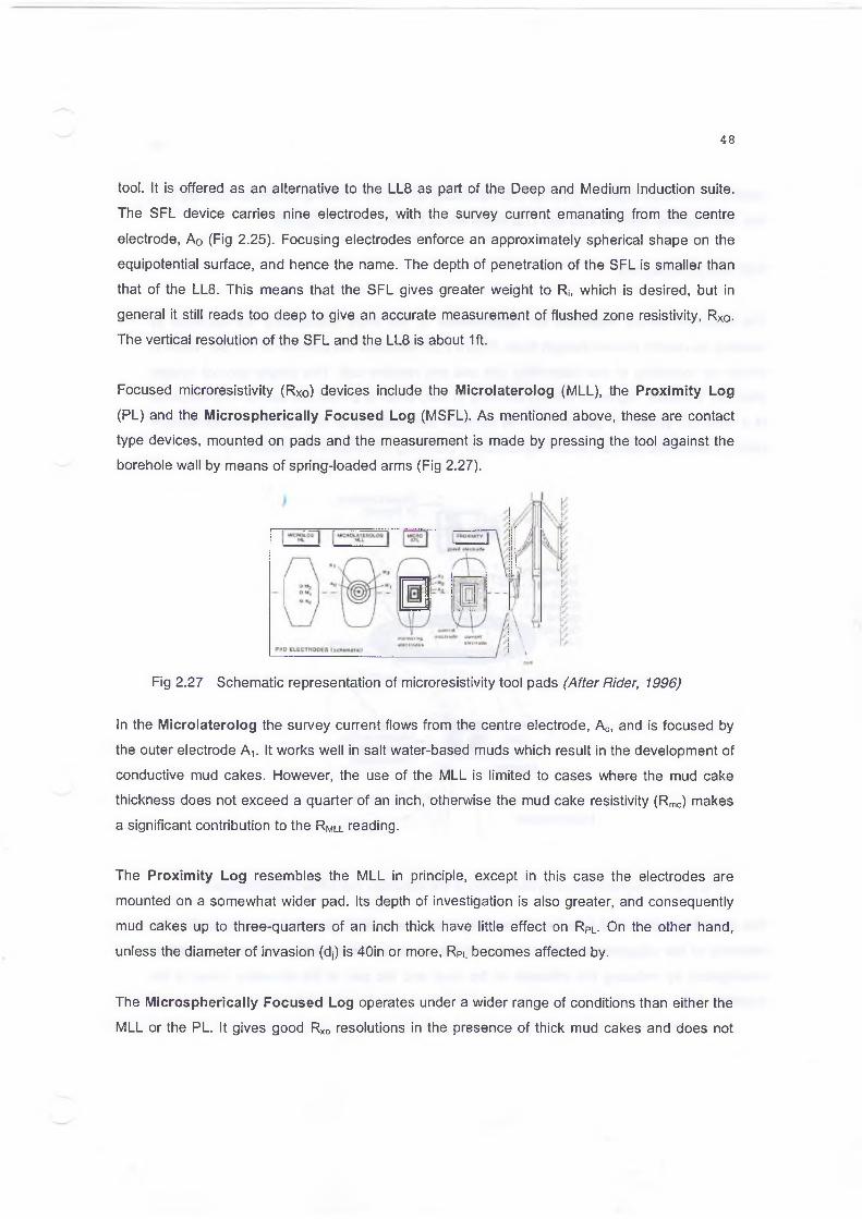
Focused microresistivity (Rxo) devices include the Microlaterolog (MLL), the Proximity Log

(PL) and the Microspherically Focused Log (MSFL). As mentioned above, these are contact

type devices, mounted on pads and the measurement is made by pressing the tool against the

borehole wall by means of spring-loaded arms (Fig 2.27).

Fig 2.27 Schematic representation of microresistivity tool pads (After Rider, 1996)

In the Microlaterolog the survey current flows from the centre electrode, A0, and is focused by

the outer electrode Av It works well in salt water-based muds which result in the development of

conductive mud cakes. However, the use of the MLL is limited to cases where the mud cake

thickness does not exceed a quarter of an inch, otherwise the mud cake resistivity ( R mc) makes

a significant contribution to the R Mll reading.

The Proximity Log resembles the MLL in principle, except in this case the electrodes are

mounted on a somewhat wider pad. Its depth of investigation is also greater, and consequently

mud cakes up to three-quarters of an inch thick have little effect on RPL. On the other hand,

unless the diameter of invasion (dj) is 40in or more, RpL becomes affected by.

The Microspherically Focused Log operates under a wider range of conditions than either the

MLL or the PL. It gives good Rxo resolutions in the presence of thick mud cakes and does not

require an invasion depth as great as that necessary for the PL. It can be combined with the DLL

tool, and together with the LLD and LLS forms the DLL-MSFL suite (Fig 2.26).

THE INDUCTION LOG

The induction device measures the conductivity of the rocks surrounding the borehole by

inducing an electric current through them. Figure 2.28 illustrates the principle of the tool, which is

shown as consisting of one transmitter coil and one receiver coil. This simple two-coil system

does not, however, represent the tool currently in use, which is a multi-coil device. The response

of a multi-coil system is derived from all possible combinations of two-coil transmitter-receiver

pairs. These responses are added algebraically, providing information on conductivity.

Receiver Coil

Secondary Magnetic _ Field "■'- - » v (Created 4 \ by the —*■'' Ground Loop)

Direct Coupling (X Signal)

Transmitter Coil

Constant Current ;

Tool movement

Primaryi , Magnetic Flux 'j (Created by 1' Transmitter) i

Fig 2.28 Diagrammatic representation of the induction tool (After Schlumberger)

The current induction tool is focused. Focusing improves vertical resolution by suppressing the

response of the adjacent beds (also known as the shoulder beds) and increases the depth of

investigation by reducing the influence of the mud and the part of the formation close to the

borehole wall.

Principle of Measurement

A constant, high frequency alternating current is sent through the transmitter coils. This

generates an alternating magnetic field which induces secondary currents (also known as

Foucault or eddy currents) in the rocks surrounding the borehole. These currents flow in circular

paths coaxial with the transmitter coils through the surrounding rocks. The resulting magnetic

field, in turn, induces signals in the receiver coils. These signals are proportional to the

conductivity of the formations from which resistivity is derived and recorded on the log.

Since the device does not require the transmission of the survey current through the mud, it can

be run in boreholes drilled with air, gas or an oil-based mud. It works well also in the presence of

conductive muds, provided the mud is not very saline, the borehole diameter is not very large

and the resistivities of the surrounding formations are less than 20 ohm-m.

Current induction systems include a deep reading device (ILD) which measures R t. and a

medium reading tool (ILM) which measures Rj. The ILD-ILM combination is called the Dual

Induction Log (DIL) and, together with a shallow Laterolog (either LL8 or SFL), is recorded in

tracks 2 and 3, forming either a DIL-LL8 or a DIL-SFL suite as shown in Figure 2.29. Normally,

an SP curve is recorded in track 1.

RECENT ADVANCES IN RESISTIVITY LOGGING

Advances have been made in recent years in both focused resitivity and induction logging. The

tools and examples of the logs are discussed below.

HIGH-RESOLUTION LATEROLOG ARRAY TOOL (HRLA)

This tool provides five independent resistivity measurements that improve R t resolution in thin

and deeply invaded formations. Enhanced focusing ensures that all signals are measured at the

same time and tool position, producing depth- and resolution-matched measurements.

Automatic corrections are carried out for borehole, shoulder or adjacent bed and invasion,

effects, yielding a more robust Rt.

The tool operates in six different ‘modes’ and delivers an array of five resitivity curves (RLA1-

SP 0.2

- 1 6 0 5 V_____________ GR0 API anils....................1 50 0 .2

40 Feet 0.2 MD

IL D _ohm-m

_ILM_ohm-mSFLU

2000

'2000

ohm-m 2000

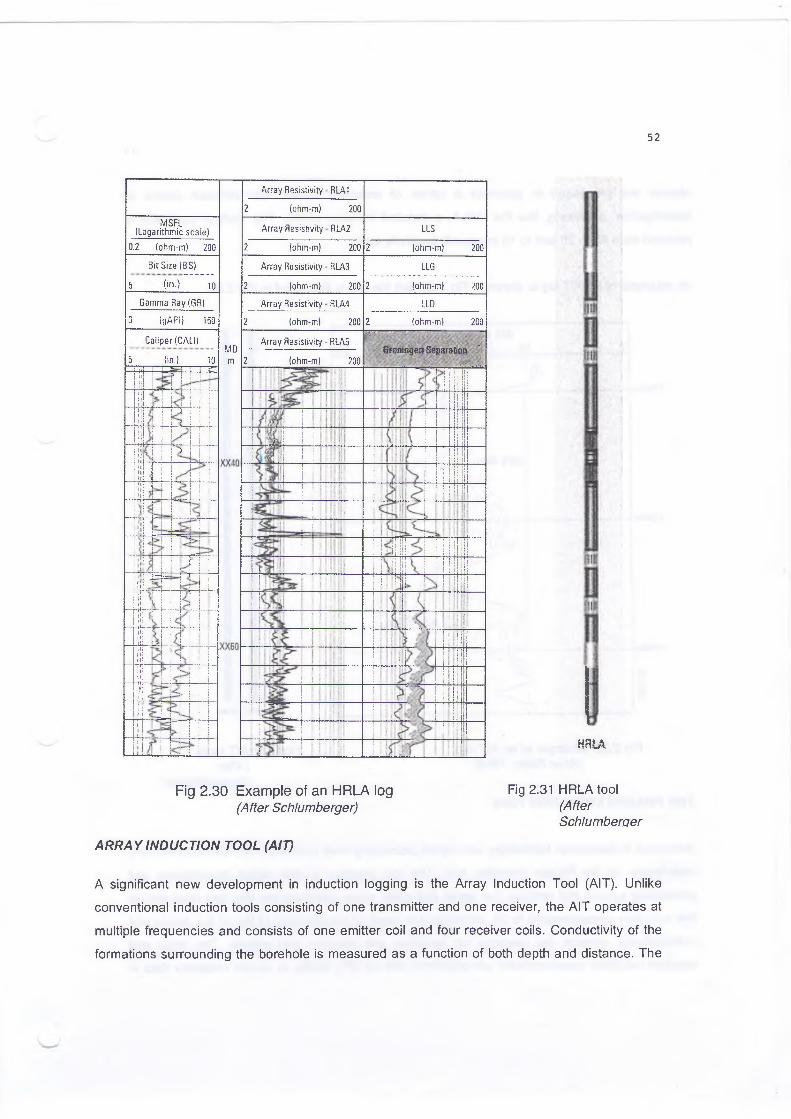
RLA5 in Fig 2.30), each with increasing depth of investigation - RLA1 < RLA2 < RLA3 < RLA4 <

RLA5 - providing a detailed resistivity profile. The resistivity curve produced in Mode 0, not

shown in Fig 2.30, primarily represents the borehole environment and is used to estimate Rm.

Fig 2.31 shows an illustration of the HRLA tool.

НЯ L A

Fig 2.30 Example of an HRLA log Fig 2.31 HRLA tool(After Schlumberger) (After

Schlumberger

ARRAY INDUCTION TOOL (AIT)

A significant new development in induction logging is the Array Induction Tool (AIT). Unlike

conventional induction tools consisting of one transmitter and one receiver, the AIT operates at

multiple frequencies and consists of one emitter coil and four receiver coils. Conductivity of the

formations surrounding the borehole is measured as a function of both depth and distance. The

Array Resistivity RLA1

2 (ohm-m) 200MSFl

(Logarithmic scale) Array Resistivity RIA2 LLS

0.2 (ohm-m) 200 2 (ohm-m) 200 2 (ohm-m) 200

Bit Size IBS) Array Resistivity RLA3 LLG

5 (in.) 10 2 (ohm-m) 200 2 (ohm-m) 200Gamma Ray(GR) Array Resistivity RLA4 LLD

0 SgAPI) 150 2 (ohm-m) 200 2 (ohm-m) 200

Caliper (CALI)MDm

Array Resistivity RLA5 ЩGromngert Separation

V . . . .....Ц

-

5 (in.) 10 ........... C_

2 (ohm-m) 200 :

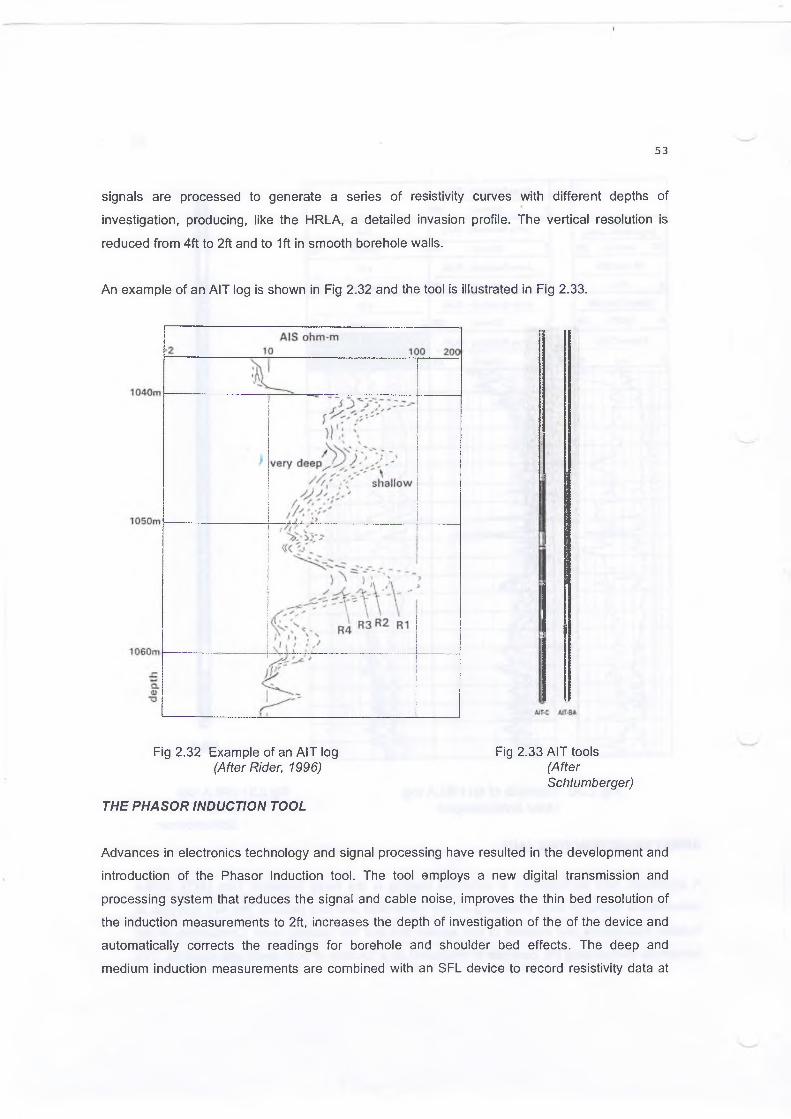
signals are processed to generate a series of resistivity curves with different depths of

investigation, producing, like the HRLA, a detailed invasion profile. The vertical resolution is

reduced from 4ft to 2ft and to 1ft in smooth borehole walls.

An example of an AIT log is shown in Fig 2.32 and the tool is illustrated in Fig 2.33.

Fig 2.32 Example of an AIT log Fig 2.33 AIT tools(After Rider, 1996) (After

Schlumberger)

THE PHASOR INDUCTION TOOL

Advances in electronics technology and signal processing have resulted in the development and

introduction of the Phasor Induction tool. The tool employs a new digital transmission and

processing system that reduces the signal and cable noise, improves the thin bed resolution of

the induction measurements to 2ft, increases the depth of investigation of the of the device and

automatically corrects the readings for borehole and shoulder bed effects. The deep and

medium induction measurements are combined with an SFL device to record resistivity data at

three depths of investigation, one curve representing R t and two reading R i.

IDPH is the deep Phasor Induction log ( R t) and IMPH the medium Phasor Induction log (R i) . The

Phasor-SFL combination may also include an SP electrode.

Fig 2.34 shows the improvement gained by Phasor processing over the conventional Induction

measurement.

Fig 2.34 Comparison between the responses of the traditional ILD and IDPH curves to Rt (After Schlumberger)

CASED HOLE FORMATION RESISTIVITY TOOL (CHFR)

Although the need to measure resistivity through casing has long been recognized, only very

recent advances in electronics technology have made this possible. Using a 12-electrode

configuration, the CHFR tool delivers a deep resistivity measurement. The tool operates in

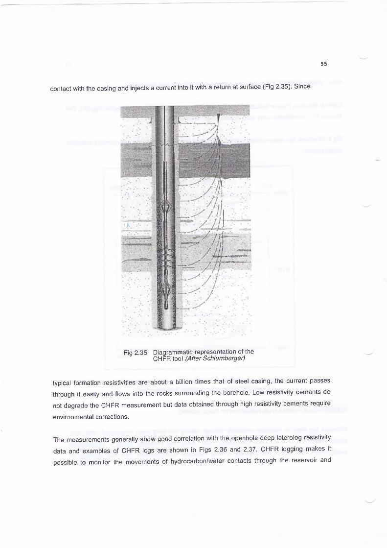
contact with the casing and injects a current into it with a return at surface (Fig 2.35). Since

Fig 2.35 Diagrammatic representation of the CHFR tool (After Schlumberger)

typical formation resistivities are about a billion times that of steel casing, the current passes

through it easily and flows into the rocks surrounding the borehole. Low resistivity cements do

not degrade the CHFR measurement but data obtained through high resistivity cements require

environmental corrections.

The measurements generally show good correlation with the openhole deep laterolog resistivity

data and examples of CHFR logs are shown in Figs 2.36 and 2.37. CHFR logging makes it

possible to monitor the movements of hydrocarbon/water contacts through the reservoir and

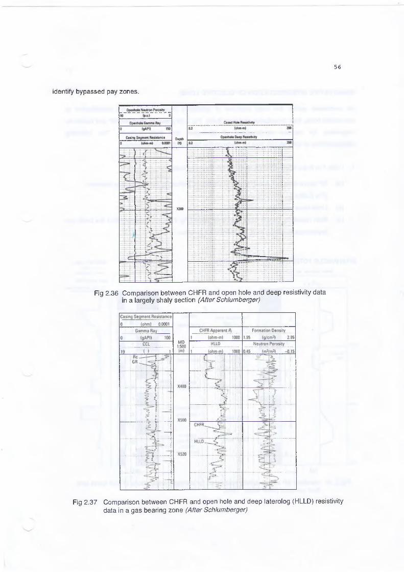
identify bypassed pay zones.

Fig 2.36 Comparison between CHFR and open hole and deep resistivity data in a largely shaly section (After Schlumberger)

Fig 2.37 Comparison between CHFR and open hole and deep laterolog (HLLD) resistivity data in a gas bearing zone (After Schlumberger)

QUALITATIVE INTERPRETATION OF ELECTRIC LOGS

As mentioned earlier, the main objective of qualitative interpretation is the identification of

permeable beds, their boundaries and pore fluids. Fig 2.38 presents idealized SP and resistivity

responses for various combinations of lithologies and fluid contents. The following

interpretations of units shown may be made on the basis of their log responses:

1. Units 1 to 6 are interpreted as shale for the following reasons:

(a) SP curve does not depart from the shale line, indicating non-permeable intervals

[Fig 2.38(a)],

(b) Units have relatively low resistivity.

(c) Both resistivity curves have the same value [Fig 2.38(b)], indicating that the beds are

impervious to drilling mud, i.e. there is no invasion.

SPONTANEOUS POTENTIALScale: M illivo lts MV

25m

I

1 I

A

4S h a leline в :

3 ic E

4

/” |

d :

5 1

:x:‘: l_

■

Permeable bedR - salt

-VR , - fresh

Permeable bedRw - fresh R , - salt

Impermeable bed

Shaly sand

R. < R...

Clean sand

RESISTIVITY LOGS----------deep---------- shallow

Scale: оИгм/т2/т(Ш

(a) (b)

OIL

SALT

POROUS•SANDSTONE

TIGHT SANDSTONE

* 'QUARTZITE'

FINING UP SHALY •SANDSTONE,

POROUS, CLEAN SALT WATER

SHALE

POROUS•SANDSTONE

POROUS

•SANDSTONE

Fig 2.38 Idealised SP and resistivity responses for various combinations of rock types and fluid contents (After Rider, 1996)

2. Unit A is interpreted as a salt water bearing sandstone for the following reasons:

(a) SP has a strong negative departure from the shale line, indicating R w < Rmff Cl

[Fig 2.38(a)], '

(b) Shallow resistivity curve shows a higher value than deep resistivity since the part of

formation investigated by the latter (uninvaded zone) is filled with conductive salty

formation water [Fig 2.38(b)].

3. Unit В is interpreted as a fresh water bearing sandstone for the following reasons:

(a) SP has a positive departure from the shale line, indicating R w > Rmf [Fig 2.38(a)],

(b) Both resistivity curves show high values as fresh water is a poor conductor [Fig

2.38(b)]. Deep resistivity curve reads higher than shallow resisttvity since the part of

formation investigated by the former (uninvaded zone) is filled with low conductivity

fresh water. )

4. Unit С is interpreted as an impermeable (tight), dry (no pore fluids) unit for the following

reasons:(a) SP does not depart from the shale line, indicating no movement of ions, i.e. no

formation water [Fig 2.38(a)].

(b) Resistivity curves track each other and show very high values indicating a non

conductive, dry formation [Fig 2.38(b)],

5. The upper part of unit D is interpreted as a shaly sandstone for the following reasons:

(a) SP curve has a reduced amplitude compared to the underlying clean sand section [Fig

2.38(a)], The gradual upward amplitude reduction reflects a progressive decrease in

grain size, indicating an upward fining sequence and a transitional contact with the

overlying shale.(b) The resistivity curves show some separation compared to shale [Fig 2.38(b)].

6. The upper part of unit E is interpreted as containing hydrocarbons and the lower part as salt

water bearing for the following reasons:

(a) Resistivity curves show high values as hydrocarbons are a poor conductor[Fig 2.38(b)].

(b) Deep resistivity shows a higher reading since the part of formation investigated by the

device (uninvaded zone) is filled with non conductive hydrocarbons.

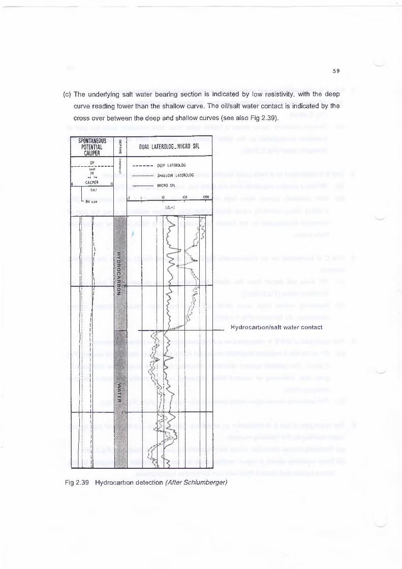
(c) The underlying salt water bearing section is indicated by low resistivity, with the deep

curve reading lower than the shallow curve. The oil/salt water contact is indicated by the

cross over between the deep and shallow curves (see also Fig 2.39).

SPONTANEOUSPOTENTIALCALIPER

(mVt20

4 — U

8 C A L I P E R 16

( in !

^ S it sue

DUAL LATEROLOG .MICRO SFL

DEEP LATEROLOG

SHALLOW LATEROLOG

MICRO SFL

100— 1000 "r—1iflm)

Hydrocarbon/salt water contact

Fig 2.39 Hydrocarbon detection (After Schlumberger)

3. THE BOREHOLE COMPENSATED (BHC) SONIC LOG

The conventional Sonic or Acoustic log provides a continuous record of the time taken, in

microseconds per foot (^sec/ft) or microseconds per metre ((isec/m), by a sound wave to travel

through one foot or one metre of formation. This is known as the interval transit time,

abbreviated to t or At. The travel time measured is that of a compressional or ‘P’ wave which

travels the fastest through the formations and represents the first arrival. Shear and Stoneley

waves follow the P waves but are not recorded by the conventional tools. Fig 3.1 shows the full

sonic wave form and an example of the arrival times of the various sonic waves is presented in

The velocity of sound through a given formation is a function of its lithology and porosity. Dense,

low porosity rocks are characterised by high matrix velocities (Vma), while porous and less dense

formations are characterised by low Vma values. Since t and Vma are inversely related, high

porosities correspond to high t values and low porosities to low t values. The conventional Sonic

log that records the P wave arrivals is therefore a porosity measuring device. Listed in Table 1

are the Vma and tma ranges of some of the most commonly encountered rock types and casing.

Fig 3.2.

Travel time (psec/ft)

Fig 3.2 Arrival times of various sonic waves (After Schlumberger)

Modern sonic tools are of the BHC (borehole compensated) type in which automatic corrections

Table 3.1 Some typical sonic matrix velocities and travel times

Vma (ft/sec) t m a (И-S e C /ft)t m a ( jA S e c /f t )

(commonly used)

Sandstone (Ф=0) 18,000-19,500 55.5-51.0 55.5 or 51.0

Limestone (Ф=0) 21,000-23,000 47.6-43.5 47.5

Dolomite (Ф=0) 23,000 43.5 43.5

Anhydrite (Ф=0) 20,000 50 50

Salt (Ф=0) 15,000 66.7 67

Casing (Ф=0) 17,500t ..

57 57

are applied to the log reading for the effects of changes in borehole size as well as for errors

arising from the tilting of the device during the logging operation.

Fig 3.3 is a schematic representation of the BHC Sonic tool, which consists of a pair of

3 '

Fig 3.3 Diagrammatic representation BHC Sonic tool (After Rider, 1996)

transmitters and two pairs of receivers. The transmitters are puised alternately, and t values are

read on alternate pairs of receivers. When one of the transmitters is pulsed, the sound wave

generated passes first into the mud and then enters the formation, travelling through the

formation close to the borehole wall. At a critical (lower) velocity it is refracted back into mud and

reaches the tool again where it is detected. The time elapsed between the detection of the first

arrival at the two corresponding receivers is measured and represents the formation reading.

The ray paths in Fig 3.3 indicate the course followed by the first arrivals of compressional sound

energy. Sound waves also travel directly between the transmitters and the receivers through the

mud. However, since the velocity of sound is greater in the formations surrounding the borehole

than in the mud due to the higher density of the former, the first arrivals are from the borehole

wall. The measured travel times of the upgoing and the downgoing signals are averaged and

this is presented linearly as the t curve.

The Schlumberger BHC tool has a spacing of 3ft between transmitter and near receiver and a

span of 2ft between receivers. The transmitters are pulsed a total of 20 times per second so that

five complete measurements are made each second. Logging speed is 5,000ft/hr, which means

a measurement is made about every 3in of hole. Normally, the Sonic tool is run centred so the

contributions to a receiver signal from different sides of the hole will be in phase (if the hole is

round) and the signal-noise ratio will be maximized. The tool can be run off centre, but

significant degradation in the signal-noise ratio must be tolerated.

LOG PRESENTATION

Typical presentation of the Sonic log, when run by itself, is shown in Fig 3.4. The interval transit

time, in microseconds per foot, is recorded across tracks 2 and 3. Short transit times are to the

right and long transit times are to the left, such that increase in porosity deflects the curve

toward the depth track consistent with Density and Neutron recording.

In the depth track are small pips, representing integrated travel time of 1 msec between each

pip. Larger pips are recorded at 10 msec intervals. These are useful in comparing Sonic logs

with seismic sections and assist in converting seismic travel times into depths. When a Gamma

Ray log is run simultaneously, it is also recorded in track 1. A resistivity tool is also run

simultaneously and the resistivity curves are displayed in track 2 and the Sonic travel time is

restricted to track 3.

Fig 3.4 BHC Sonic log presentation (After Baker Atlas)

A good check on the accuracy of a Sonic log is to observe the reading in casing. It should be 57

S^sec/ft, the travel time of steel. The log may not jump immediately to this value on entering

casing because there can be a drastic change in signal amplitude to which the system (or the

engineer) must adjust. The reading is most reliable in uncemented pipe where the casing-borne

arrival will have good amplitude and will always arrive ahead of formation-borne signals, no

matter how fast. The opposite can be true in cemented pipe.

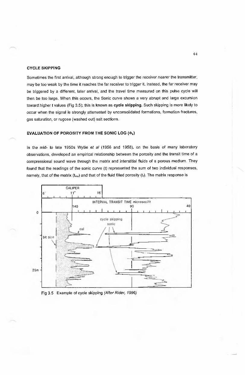
CYCLE SKIPPING

Sometimes the first arrival, although strong enough to trigger the receiver nearer the transmitter,

may be too weak by the time it reaches the far receiver to trigger it. Instead, the far receiver may

be triggered by a different, later arrival, and the travel time measured on this pulse cycle will

then be too large. When this occurs, the Sonic curve shows a very abrupt and large excursion

toward higher t values (Fig 3.5); this is known as cycle skipping. Such skipping is more likely to

occur when the signal is strongly attenuated by unconsolidated formations, formation fractures,

gas saturation, or rugose (washed out) salt sections.

EVALUATION OF POROSITY FROM THE SONIC LOG (Ф5)

In the mid- to late 1950s Wyllie et al (1956 and 1958), on the basis of many laboratory

observations, developed an empirical relationship between the porosity and the transit time of a

compressional sound wave through the matrix and interstitial fluids of a porous medium. They

found that the readings of the sonic curve (t) represented the sum of two individual responses,

namely, that of the matrix (tma) and that of the fluid filled porosity (tf). The matrix response is

Fig 3.5 Example of cycle skipping (After Rider, 1996)

given by the amount of matrix (1 - Ф) multiplied by tma, and the fluid filled contribution equals the

amount of fluid (Ф) multiplied by tf. Thus:

t=(1-4>)tma+<Mf 3.1

Solving for Ф:

Ф5 = (t - tma)/(tr tma) 3.2

This is known as the time-average equation, and has been used universally to derive sonic

porosities from the log-recorded travel time, t, provided tf and t™a are known. The fluid in the

zone of investigation is typically mud filtrate. Consequently, tf is normally taken as 189 (.isec/ft in

fresh mud. In salt mud a value of 185 jisec/ft may be used. Matrix travel times vary from 40-50

^sec/ft, depending on lithology.

Fig 3.6 presents a graphical solution to equation 3.2. Log-derived transit time is entered on the

horizontal axis, a line is projected vertically to the appropriate matrix velocity, and porosity is

read on the vertical scale opposite the point of intersection.

As an example, the zone at XX869 - XX874 ft in Fig 3.4 reads a travel time of 71 [isec/ft. Using

the straight, continuous blue lines. Fig 3.6 gives a porosity of 12% if the matrix is sandstone or

as high as 22% if the matrix is dolomite. Clearly, the lithology must be known to obtain accurate

porosity values. Even within the given lithology there is a range of possible matrix travel times,

as indicated by straight continuous lines in Fig 3.6. Local knowledge dictates the value to use -

although the deeper the burial of a formation, the lower tma is likely to be.

Effects of Under-compaction on Ф5

The time-average relation holds quite well in consolidated or well-compacted formations.

Typically, these have transit times less than 100 usec/ft. However, serious errors arise if the

relation is applied without modification in shallow, unconsolidated sands which occur in

geologically younger formations. If the effective pressure on the rock framework

(overburden-hydrostatic) is less than about 4,000 psi, which is the case at depths less than

about 2,000m, the sand has not reached its fully compacted rigidity. Travel times in

uncompacted sands may reach as much as 150 ^sec/ft, which convert to porosities far above

v, =-5300 ft/sec

30 40 50 60 V0 80 90 100 110 120 130

L, interval transit time ((isec/tt)

Fig 3.6 Porosity evaluation from the Sonic log (After Schlumberger)

the known maximum of 40%. In such cases, the porosity computed from equation 3.2 must be

divided by a compaction correction factor, Bcp, as indicated in Fig 3.6. The factor varies from

1.0 to as high as 1.8. Bcp is never less than unity. Equation 3.2 thus becomes:

<£>S = ( t - t m a ) / ( t f - La) x 1/Bcp 3.3

Typical sonic compaction factors are listed in Table 3.2.

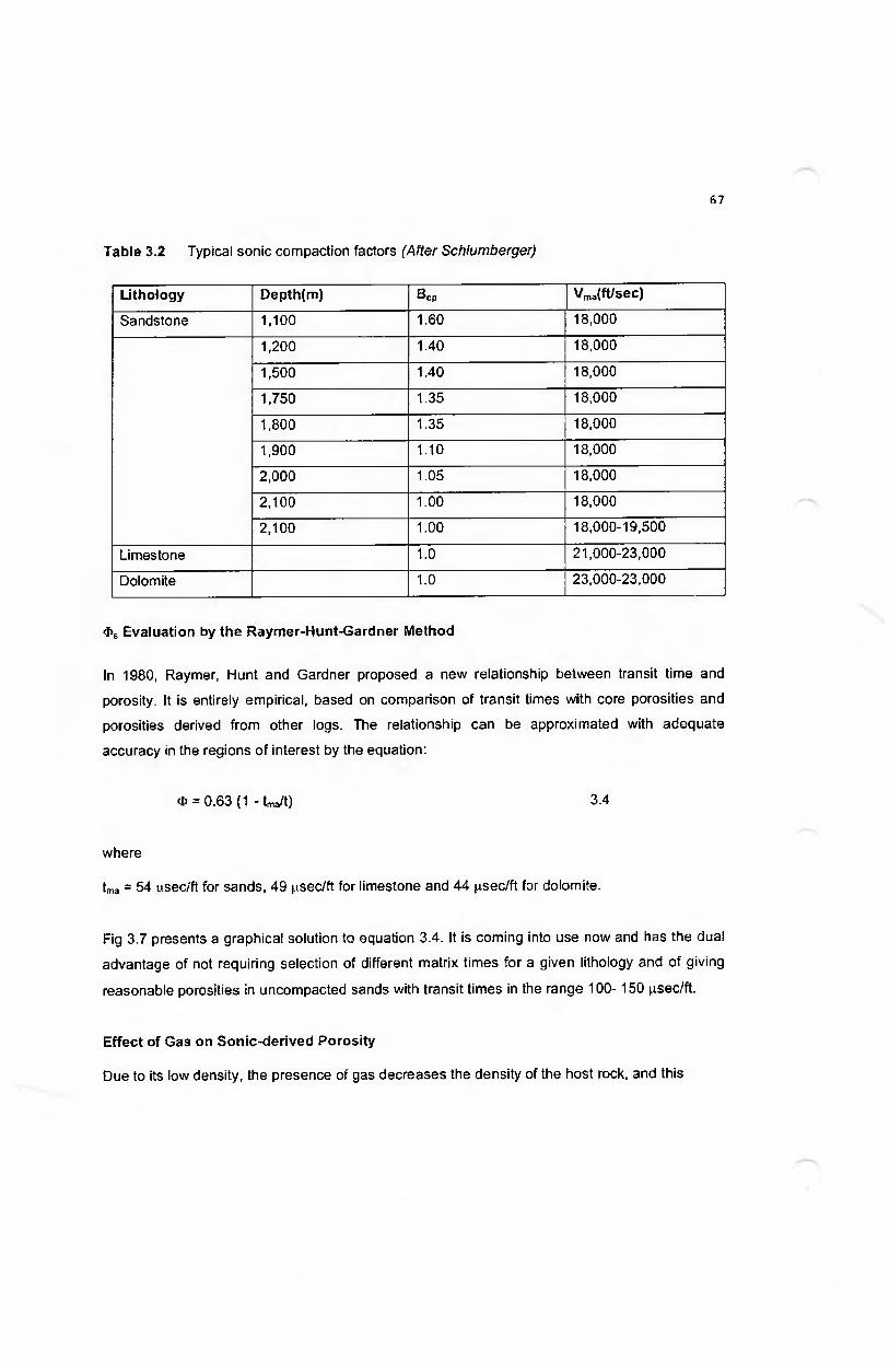
Table 3.2 Typical sonic compaction factors (After Schlumberger)

Lithology Depth(m) Bcp Vma(ft/sec)

Sandstone 1,100 1.60 18,000

1,200 1.40 18,000

1,500 1.40 18,000

1,750 1.35 18,000

1,800 1.35 18,000

1,900 1.10 18,000

2,000 1.05 18,000

2,100 1.00 18,000

2,100 1.00 18,000-19,500

Limestone 1.0 21,000-23,000

Dolomite 1.0 23,000-23,000

Ф5 Evaluation by the Raymer-Hunt-Gardner Method

In 1980, Raymer, Hunt and Gardner proposed a new relationship between transit time and

porosity. It is entirely empirical, based on comparison of transit times with core porosities and

porosities derived from other logs. The relationship can be approximated with adequate

accuracy in the regions of interest by the equation:

Ф = 0.63(1 -tma/t) 3.4

where

tma = 54 usec/ft for sands, 49 |.isec/ft for limestone and 44 ^sec/ft for dolomite.

Fig 3.7 presents a graphical solution to equation 3.4. It is coming into use now and has the dual

advantage of not requiring selection of different matrix times for a given lithology and of giving

reasonable porosities in uncompacted sands with transit times in the range 100-150 usec/ft.

Effect of Gas on Sonic-derived Porosity

Due to its low density, the presence of gas decreases the density of the host rock, and this

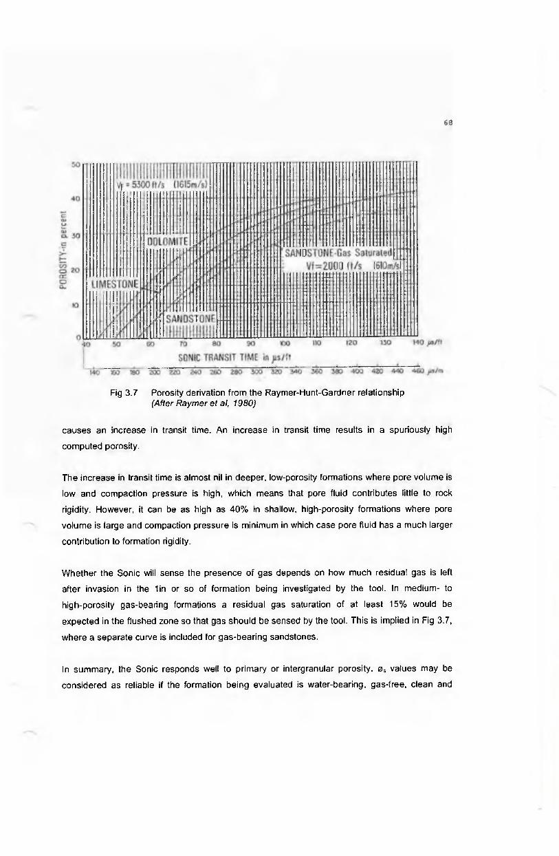
Fig 3.7 Porosity derivation from the Raymer-Hunt-Gardner relationship (After Raymer et al, 1980)

causes an increase in transit time. An increase in transit time results in a spuriously high

computed porosity.

The increase in transit time is almost nil in deeper, low-porosity formations where pore volume is

low and compaction pressure is high, which means that pore fluid contributes little to rock

rigidity. However, it can be as high as 40% in shallow, high-porosity formations where pore

volume is large and compaction pressure is minimum in which case pore fluid has a much larger

contribution to formation rigidity.

Whether the Sonic will sense the presence of gas depends on how much residual gas is left

after invasion in the 1 in or so of formation being investigated by the tool. In medium- to

high-porosity gas-bearing formations a residual gas saturation of at least 15% would be

expected in the flushed zone so that gas should be sensed by the tool. This is implied in Fig 3.7,

where a separate curve is included for gas-bearing sandstones.

In summary, the Sonic responds well to primary or intergranular porosity. os values may be

considered as reliable if the formation being evaluated is water-bearing, gas-free, clean and

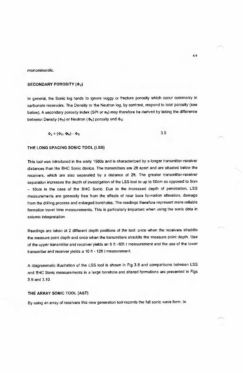
monomineralic.

SECONDARY POROSITY (Ф2)

In general, the Sonic log tends to ignore vuggy or fracture porosity which occur commonly in

carbonate reservoirs. The Density or the Neutron log, by contrast, respond to total porosity (see

below). A secondary porosity index (SPI or a2) may therefore be derived by taking the difference

between Density (Фо) or Neutron (Фм) porosity and Фэ:

ф2 = (Фо, Фц) - Os 3.5

THE LONG SPACING SONIC TOOL (LSS)

This tool was introduced in the early 1980s and is characterized by a longer transmitter-receiver

distances than the BHC Sonic device. The transmitters are 2ft apart and are situated below the

receivers, which are also separated by a distance of 2ft. The greater transmitter-receiver

separation increases the depth of investigation of the LSS tool to up to 50cm as opposed to 5cm

- 10cm in the case of the BHC Sonic. Due to the increased depth of penetration, LSS

measurements are generally free from the effects of near bore formation alteration, damage

from the drilling process and enlarged boreholes. The readings therefore represent more reliable

formation travel time measurements. This is particularly important when using the sonic data in

seismic interpretation.

Readings are taken at 2 different depth positions of the tool: once when the receivers straddle

the measure point depth and once when the transmitters straddle the measure point depth. Use

of the upper transmitter and receiver yields an 8 ft -10ft t measurement and the use of the lower

transmitter and receiver yields a 10 ft - 12ft t measurement.

A diagrammatic illustration of the LSS tool is shown in Fig 3.8 and comparisons between LSS

and BHC Sonic measurements in a large borehole and altered formations are presented in Figs

3.9 and 3.10.

THE ARRAY SONIC TOOL (AST)

By using an array of receivers this new generation tool records the full sonic wave form. In

illh\ s

T — transm itter L — l o w e r U — u p p e r

R r e c e i v e r

Fig 3.8 Diagrammatic representation of the Long Spacing Sonic tool (After Rider, 1996)

addition to recording the arrival times of the P waves, the AST measures the shear and Stoneley

wave arrivals. The tool produces data for specialist applications and is not run as part of the

standard suite of logs.

Applications o f AST Data

The main application of AST data is to the determination of the rock mechanical properties

which serve as a useful aid in the interpretation of seismic data. These properties include the

Poisson’s ratio, Young’s modulus, shear modulus and the bulk compressibility of the formations

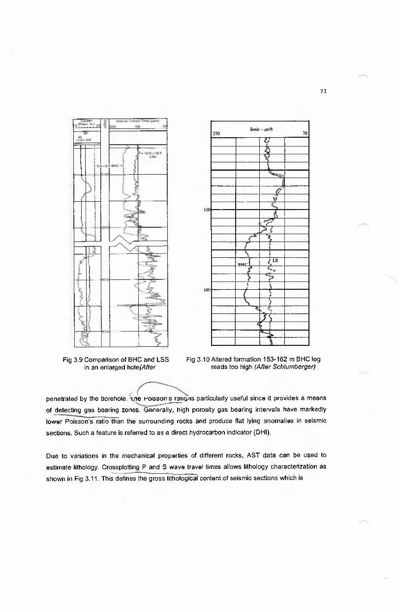
Fig 3.9 Comparison of BHC and LSS Fig 3.10 Altered formation 153-162 m BHC log in an enlarged hole (After reads too high (After Schlumberger)

penetrated by the borehole. V n C ^ isso n ^ 'a n Q is particularly useful since it provides a means

of detecting gas bearing zones. Generally, high porosity gas bearing intervals have markedly

lower Poisson’s ratio than the surrounding rocks and produce flat lying anomalies in seismic

sections. Such a feature is referred to as a direct hydrocarbon indicator (DHI).

Due to variations in the mechanical properties of different rocks, AST data can be used to

estimate lithology. Crossplotting P and S wave travel times allows lithology characterization as

shown in Fig 3.11. This defines the gross lithological content of seismic sections which is

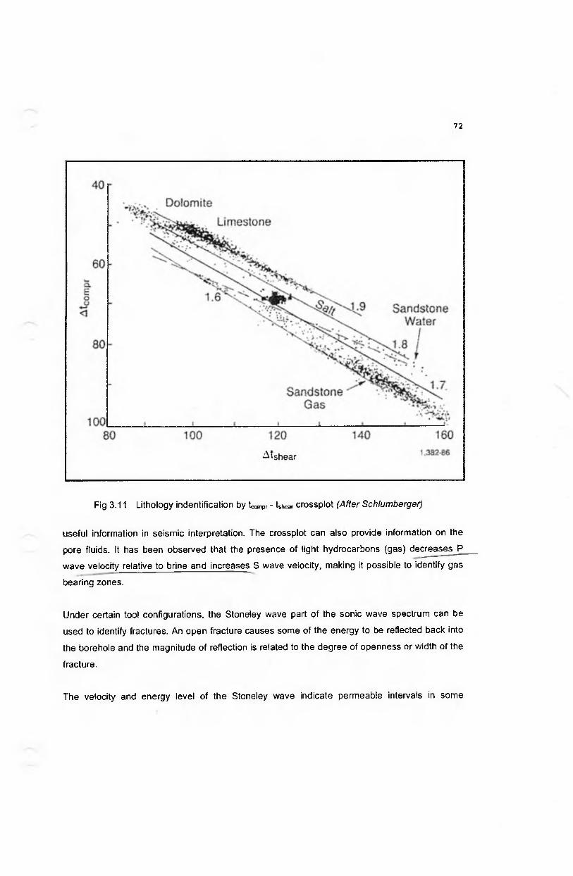
Fig 3.11 Lithology indentification by tcompr - tshear crossplot (After Schlumberger)

useful information in seismic interpretation. The crossplot can also provide information on the

pore fluids. It has been observed that the presence of light hydrocarbons (gas) decreases P

wave velocity relative to brine and increases S wave velocity, making it possible to identify gas

bearing zones.

Under certain tool configurations, the Stoneley wave part of the sonic wave spectrum can be

used to identify fractures. An open fracture causes some of the energy to be reflected back into

the borehole and the magnitude of reflection is related to the degree of openness or width of the

fracture.

The velocity and energy level of the Stoneley wave indicate permeable intervals in some

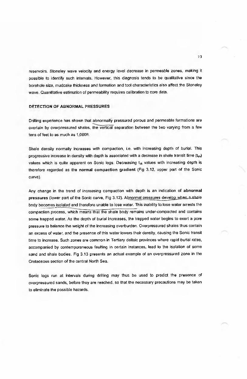
reservoirs. Stoneley wave velocity and energy level decrease in permeable zones, making it

possible to identify such intervals. However, this diagnosis tends to be qualitative since the

borehole size, mudcake thickness and formation and tool characteristics also affect the Stoneley

wave. Quantitative estimation of permeability requires calibration to core data.

DETECTION OF ABNORMAL PRESSURES

Drilling experience has shown that abnormally pressured porous and permeable formations are

overlain by overpressured shales, the vertical separation between the two varying from a few

tens of feet to as much as 1,000ft.

Shale density normally increases with compaction, i.e. with increasing depth of burial. This

progressive increase in density with depth is associated with a decrease in shale transit time (tsn)

values which is quite apparent on Sonic logs. Decreasing t5h values with increasing depth is

therefore regarded as the normal compaction gradient (Fig 3.12, upper part of the Sonic

curve).

Any change in the trend of increasing compaction with depth is an indication of abnormal

pressures (lower part of the Sonic curve, Fig 3.12). Abnormal pressures develop when-a-sbale

body becomes isolated and therefore unable to lose water. This inability to lose water arrests the

compaction process, which means that the shale body remains under-compacted and contains

some trapped water. As the depth of burial increases, the trapped water begins to exert a pore

pressure to balance the weight of the increasing overburden. Overpressured shales thus contain

an excess of water, and the presence of this water lowers their density, causing the Sonic transit

time to increase. Such zones are common in Tertiary deltaic provinces where rapid burial rates,

accompanied by contemporaneous faulting in certain instances, lead to the isolation of some

sand and shale bodies. Fig 3.13 presents an actual example of an overpressured zone in the

Cretaceous section of the central North Sea.

Sonic logs run at intervals during drilling may thus be used to predict the presence of

overpressured sands, before they are reached, so that the necessary precautions may be taken

to eliminate the possible hazards.

C K

ч

ч\

1

Fig 3.12 Detecting overpressured zones with the Sonic log (After Schlumberger) ^ ^

л & Л .

\ ' *.■\ (W " ? \ \

Я\ ‘ ’

A c

',\XVy/vA • J 4' Q *

Ч

и К 211/29-1

Measureddepth

(metres)

DT

400.0 (msecs/ft) 40.0

- 600

- 800

— 1000

- 1200

- 1400

- 1600

- 1800

2000

2200

- 2400

2600

2800

— 'Normal’ compaction

— trend

Overpressure

Fig 3.13 Example of overpressuring in the Cretaceous section, North Sea (Millennium Atlas, 2004)

4. RADIOACTIVE LOGS

These logs are entirely different from those discussed previously, and as their name suggests,

they utilise the radioactive or nuclear properties of the rocks surrounding the borehole. Basically,

two measurements are recorded on radioactive logs: (1) the natural gamma ray activity of the

beds; and (2) the effects of neutron or gamma ray bombardment. Radioactive logs provide

information on the lithology and porosity of the formations traversed by the borehole.

The main feature of radioactive lagging is that it is not dependent on the presence of drilling mud

in the well; it can even be carried out after the well has been cased, and this makes it possible to

re-examine the stratigraphy and recorrelate the strata in old-established fields. A

re-interpretation of the geology in this manner shows if any productive layers have been missed.

Acquisition of radioactive log data involves the measurement of the count rates of gamma rays

or certain types of neutrons and electrons. Since the count rates of nuclear particles vary in time,

logging speed has a significant effect on data quality. Fig 4.1 illustrates the effect of logging

speed on the bed boundary resolution ability of the Gamma Ray log. The best results are

obtained at lower speeds and since most tool combinations include at least one radioactive

device (usually a gamma ray recorder), all logs are run at a speed of 1,800ft/hr.

/5,400 Ft/hr/

Fig 4.1 Effect of logging speed on bed boundary resolution of the GR log (Modified from Dewan, 1983)

Radioactive logs fall into three main categories: (1) Gamma Ray log; (2) the Neutron log; and (3)

the Formation Density log.

THE GAMMA RAY (GR) LOG

This log records the natural radioactivity of formations. The radioactivity arises from the

presence of uranium (U), thorium (Th) and potassium (K40) in the rocks. These three elements

continuously emit gamma rays, which are short bursts of high energy radiation similar to x-rays.

Gamma rays are capable of penetrating a few inches of rock, and a fraction of those that

originate close to the borehole traverse the hole and can be detected by a suitable gamma-ray

sensor. The detector gives a discrete electrical pulse for each gamma ray detected, and the

parameter logged is the number of pulses recorded per unit of time by the detector. Fig 4.2

shows the relative radioactivity of various sedimentary rocks.

0 4 8 И 20 40 60 80 100

Caprock and anhydrite Coal SaltDolomite Limestone SandstoneSandy limestone and

limy sandstone Greenish-gray sandstone Shaly sandstone Shaly limestone Sandy shale Calcareous shale ShaleOrganic marine shale Lean potash beds Rich potash beds

Fig 4.2 Relative radioactivity of various sedimentary rocks (AfterBaker Atlas,1982)

GR logs are calibrated in API units (APIU), an arbitrary scale set up by the American Petroleum

Institute. The scale increases from left to right, and the log is recorded linearly on track 1. Typical

GR responses in various lithologies are illustrated in Fig 4.3 GR log presentation is shown in Fig

4.4.

Fig 4.3 Typical GR responses in various lithologies (After Schlumberger)

'

S - r

Fig 4.4 Presentation of the GR log [track 1] (After Schlumberger)

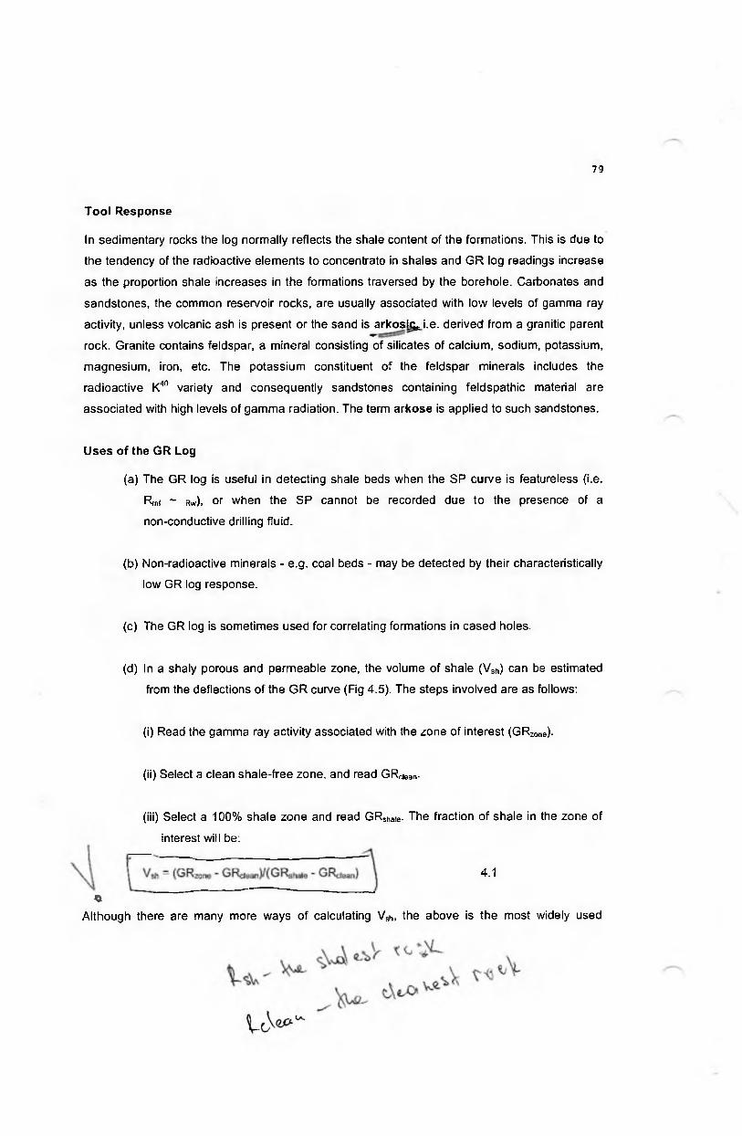
Tool Response

In sedimentary rocks the log normally reflects the shale content of the formations. This is due to

the tendency of the radioactive elements to concentrate in shales and GR log readings increase

as the proportion shale increases in the formations traversed by the borehole. Carbonates and

sandstones, the common reservoir rocks, are usually associated with low levels of gamma ray

activity, unless volcanic ash is present or the sand is arkosit^ i.e. derived from a granitic parent

rock. Granite contains feldspar, a mineral consisting of silicates of calcium, sodium, potassium,

magnesium, iron, etc. The potassium constituent of the feldspar minerals includes the

radioactive K40 variety and consequently sandstones containing feldspathic material are

associated with high levels of gamma radiation. The term arkose is applied to such sandstones.

Uses o f the GR Log

(a) The GR log is useful in detecting shale beds when the SP curve is featureless (i.e.

Rmf ~ r«). or when the SP cannot be recorded due to the presence of a

non-conductive drilling fluid.

(b) Non-radioactive minerals - e.g. coal beds - may be detected by their characteristically

low GR log response.

(c) The GR log is sometimes used for correlating formations in cased holes.

(d) In a shaly porous and permeable zone, the volume of shale (V5h) can be estimated

from the deflections of the GR curve (Fig 4.5). The steps involved are as follows:

(i) Read the gamma ray activity associated with the zone of interest (GRZOne)-

(ii) Select a clean shale-free zone, and read GRciean-

(iii) Select a 100% shale zone and read GRShaie- The fraction of shale in the zone of

interest will be:

Although there are many more ways of calculating Vsh, the above is the most widely used

4.1

О

method. ci0 2S SO 75 100

Fig 4.5 Determination of Vsh from the GR log (After Dewan, 1983)

THE NATURAL GAMMA RAY SPECTROMETRY TOOL (NGS)

The Natural Gamma Ray Spectrometry Tool (NGS) was introduced in the 1980s and represents

a new development of the conventional GR log. As shown in Fig 4.6, the NGST is a pad contact

device, held against the borehole wall by means of a bow spring.

Whereas the conventional GR log records the total radiation emitted by U238, Th232 and K40, the

NGS examines the gamma ray spectrum in more detail, detecting and recording the individual

contributions of the three radioactive elements.

This is possible since uranium, thorium and potassium emit gamma rays of different energies as

shown in Fig 4.6. Potassium has a single peak at 1.46 mev (million electron volts), while thorium

and uranium emit gamma rays of various energies, the major distinction being a prominent

Fig 4.5 Natural GR Spectrometry Tool (After Schlumberger)

thorium peak at 2.62 mev and a predominant uranium peak at about 0.6 mev. Since minerals

have characteristic concentrations of uranium, thorium and potassium, the individual responses

can sometimes be used to identify minerals or mineral type.

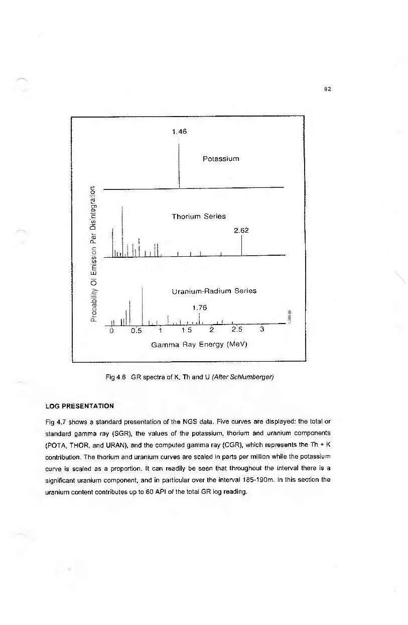
1.46

с.оcdL_CJ)О)селОшCLСОсослеш

б

-Q

_ оо

in

I I

±1

P otassium

Thorium Series

2.62

U ran ium -R ad ium S eries

1.76I . !

' ■ I . 1 I C I I ■ 1 I I _ _ _ _ _ _ _ _ _ _ _ _

0 0.5 i 1.5 2 2.5 3

G am m a Ray Energy (MeV)

Fig 4.6 GR spectra of K, Th and U (After Schlumberger)

LOG PRESENTATION

Fig 4.7 shows a standard presentation of the NGS data. Five curves are displayed: the total or

standard gamma ray (SGR), the values of the potassium, thorium and uranium components

(POTA, THOR, and URAN), and the computed gamma ray (CGR), which represents the Th + К

contribution. The thorium and uranium curves are scaled in parts per million while the potassium

curve is scaled as a proportion. It can readily be seen that throughout the interval there is a

significant uranium component, and in particular over the interval 185-190m. In this section the

uranium content contributes up to 60 API of the total GR log reading.

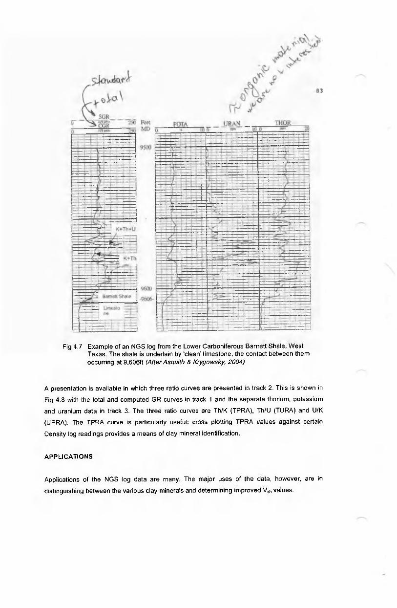
Fig 4.7 Example of an NGS log from the Lower Carboniferous Barnett Shale, West Texas. The shale is underlain by ‘clean’ limestone, the contact between them occurring at 9,606ft (After Asquith & Krygowsky, 2004)

A presentation is available in which three ratio curves are presented in track 2. This is shown in

Fig 4.8 with the total and computed GR curves in track 1 and the separate thorium, potassium

and uranium data in track 3. The three ratio curves are Th/K (TPRA), Th/U (TURA) and U/K

(UPRA). The TPRA curve is particularly useful: cross plotting TPRA values against certain

Density log readings provides a means of clay mineral identification.

APPLICATIONS

Applications of the NGS log data are many. The major uses of the data, however, are in

distinguishing between the various clay minerals and determining improved Vsh values.

Clay mineral identification may be effected by the use of the chart illustrated in Fig 4.9, which

compares the potassium and thorium contents of several minerals. The chart is entered by

taking values directly from the recorded curves. Usually the result is not unambiguous, and

consequently other data need to be introduced. In particular, the photoelectric absorption

Fig 4.8 Ratio presentation of NGS data (After Schlumberger)

£ClCL

EзT~Оs:h-

Kaolmite

•30% glauconite

GlauconiteFeldspar

Fig 4.9

1 2 3 4

Pot assi um (%)

Mineral identification from NGS log data (After Schlumberger)

Th/K: 0.Э

Potassium evapontes. -30% feldspar

Possible 100% kaolimte montmorillonite, illite “clay line" 100% illite point

coefficient (see under the Litho-Density log in this section) and the ratios of the radioactive

families are used: Th/K, U/K and Th/U.

The major occurrences of the three radioactive families are as follows:

Potassium: micas, feldspars, micaceous clays (illite), radioactive evaporites.

Thorium: shales, heavy minerals.

Uranium: phosphates, organic matter.

The significance of the type of radiation is dependent on the lithology of the formation with which

it is associated. In carbonates uranium indicates the presence of organic matter, phosphates

and stylolites, while the thorium and potassium levels are representative of the clay content, in

sandstones the thorium level is determined by the heavy minerals and clay content, and the

potassium is usually contained in micas and feldspars. In shales the potassium content is

indicative of the clay mineral type and the presence of mica, and the thorium levels is dependent

on the amount of detrital material, or the degree of shaliness. The presence of uranium would

suggest that the shale is a potential source rock, since uranium seems to be associated with

organic matter in argillaceous sediments.

In addition to lithology, the distribution of the radioactive minerals in a sedimentary formation is

dependent also on the agent and manner of transportation, the degree of reworking and

alteration. For example, due to its low solubility, Th has limited mobility and tends to accumulate

with the heavy minerals. On the other hand, uranium has a greater solubility and mobility, and so

high uranium concentrations are found along fault planes, fractures and in formations where

water flow has occurred. Similarly, high uranium concentrations can build up in producing oil

wells, in the permeable beds and on the tubing and casing. Chemical marine deposits are

characterised by their extremely low radioactive content, with none of the three radiation families

making any significant contribution.

In areas where abnormal amounts of potassium-bearing micas and feldspars are associated

with the sands (the North Sea, granite wash areas of the southwestern US), the thorium.,,

component alone is the best indicator of shale content.

As the proportion of uranium is dependent more on the organic content of shales than the

amount of clay, it is not a particularly good quantitative clay indicator. For this reason, the CGR

curve, which is the sum of the thorium and potassium components only, is a better indicator of

shliness. When a KCI mud has been used to drill the borehole the high potassium content will

affect the measurement, and so under these circumstances the thorium measurement alone will

probably be the best clay indicator.

A clay index computation can be made using any of the recorded data. Fig 4.10 is an example

comparing five clay indicators, derived from the thorium (VSTC), potassium (VSPC), uranium

(VSUC), total gamma ray (VSSG) and computed gamma ray (VSCG) data. It is evident that the

values obtained from the thorium and potassium content correlate well, but the uranium derived

curve has a very different character. The relative uranium concentrations of the two shale zones

suggest the possibility that the lower shale is an organic rich source rock.

\ 4 ' v 0

9 '

, < Ц оv>

Лt j

Fig 4.10 Comparison of 5 clay indicators computed from NGS data (After Schlumberger)

m^ vTHE NEUTRON LOG V s :

vv

v ЧК't _ /

In neutron logging the formations surrounding the borehole are bombarded by high energy

neutrons from a radioactive source in the device. The Neutron tool and its operation are

illustrated diagrammatically in Figs 4.11 and 4.12. The current second generation tools have two

detectors located above the source.

(After Dewan, 1983)

Neutrons are electrically neutral particles with a mass almost identical to that of a hydrogen

atom. On leaving the source, the neutrons enter the formations and collide with nuclei in the

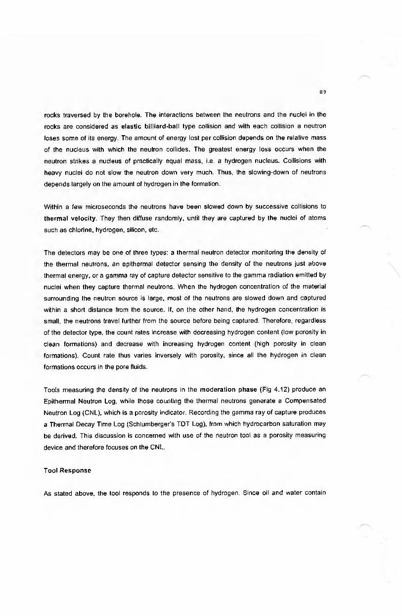
rocks traversed by the borehole. The interactions between the neutrons and the nuclei in the

rocks are considered as elastic billiard-ball type collision and with each collision a neutron

loses some of its energy. The amount of energy lost per collision depends on the relative mass

of the nucleus with which the neutron collides. The greatest energy loss occurs when the

neutron strikes a nucleus of practically equal mass, i.e. a hydrogen nucleus. Collisions with

heavy nuclei do not slow the neutron down very much. Thus, the slowing-down of neutrons

depends largely on the amount of hydrogen in the formation.

Within a few microseconds the neutrons have been slowed down by successive collisions to

thermal velocity. They then diffuse randomly, until they are captured by the nuclei of atoms

such as chlorine, hydrogen, silicon, etc.

The detectors may be one of three types: a thermal neutron detector monitoring the density of

the thermal neutrons, an epithermal detector sensing the density of the neutrons just above

thermal energy, or a gamma ray of capture detector sensitive to the gamma radiation emitted by

nuclei when they capture thermal neutrons. When the hydrogen concentration of the material

surrounding the neutron source is large, most of the neutrons are slowed down and captured

within a short distance from the source. If, on the other hand, the hydrogen concentration is

small, the neutrons travel further from the source before being captured. Therefore, regardless

of the detector type, the count rates increase with decreasing hydrogen content (low porosity in

clean formations) and decrease with increasing hydrogen content (high porosity in clean

formations). Count rate thus varies inversely with porosity, since all the hydrogen in clean

formations occurs in the pore fluids.

Tools measuring the density of the neutrons in the moderation phase (Fig 4.12) produce an

Epithermal Neutron Log, while those counting the thermal neutrons generate a Compensated

Neutron Log (CNL), which is a porosity indicator. Recording the gamma ray of capture produces

a Thermal Decay Time Log (Schlumberger’s TDT Log), from which hydrocarbon saturation may

be derived. This discussion is concerned with use of the neutron tool as a porosity measuring

device and therefore focuses on the CNL.

Tool Response

As stated above, the tool responds to the presence of hydrogen. Since oil and water contain

practically the same amount of hydrogen per unit volume, the responses reflect primarily the

liquid-filled porosity in clean formations. The tool does not, however, distinguish between the

hydrogen in the pore fluids and that associated with bound water, i.e. water of crystallisation.

The latter, of course, does not always correspond to effective porosity; for example, shales and

gypsum (Ca S04.2H20) containing bound water have a high hydrogen index, and are therefore

characterised by a large 'neutron porosity'. In general, however, dense and non-porous beds

such as anhydrite and tight limestones are indicated by low porosity peaks on the neutron curve,

while porous zones show higher readings.

The device is calibrated by using a standard piece of fresh water-bearing, pure limestone in the

American Petroleum Institute (API) test laboratories. Consequently, the porosities recorded

normally assume that the matrix is limestone. The logs are therefore scaled in 'Limestone

Porosity Units'.

If the matrix happens to be sandstone, the true porosity will be different by about 4 p.u., i.e., 20 p

u sandstone will register as 16 limestone p u. The effects are evident in Fig 4.13, which can be

used also to estimate porosity in clean, water-bearing and gas-free zones consisting of a single

lithology.

e-Miro.-. apparent limestone neutron porosi’y (p 11.)

Fig 4.13 Thermal neutron porosity equivalence curves (After Schlumberger)

Liquid hydrocarbons have hydrogen indexes close to that of water. Gas, however, usually has a

considerably lower hydrogen concentration, which varies with temperature and pressure.

Therefore, when gas is present near enough the borehole to be within its zone of investigation, a

Neutron Log reads too low a porosity. This characteristic is called the gas effect, and allows the

Neutron Log to be used to detect gas zones; in a formation known to have uniform porosity, the

Neutron Log alone will often indicate gas/liquid contacts. A Neutron and Density log combination

is more effective in identifying gas bearing formations and allows gas detection in a zone with

variable porosity, a more accurate quantification of porosity and eliminating the effect of shale.

The CNL has a radius of investigation of about 10in. If run slowly, the vertical resolution of the

tool is approximately 2ft.

Log Presentation

The CNL is rarely run by itself because of substantial matrix and clay effects. It is normally run in

combination with the Compensated Density and GR logs in the configuration shown in Fig 1.5

(bottom right-hand diagram). The Neutron is positioned above the Density with its backup spring

lined up with that of the Density so that the array is forced against the same side of the hole.

Fig 4.14 shows the standard presentation of the curves obtained with the Neutron-Density

combination. A GR log, caliper and bit size are recorded in track 1, and Neutron and Density

curves in tracks 2 and 3 with the Neutron curve dashed and the Density solid. The CNL curve is

scaled in porosity units, each division corresponding to 3 p u.

Evaluation of Porosity From the CNL

The CNL reads the total porosity. In a monomineraiic, clean (shale-free), water bearing and

gas-free permeable zone, the log reading can be converted directly into a true porosity value

provided the lithology is known, as shown in the chart in Fig 4.13. The dashed lines are for

porosity determination from the Sidewall Neutron Porosity (SNP) tool, which is now obsolete.

With the increasing use of LWD in field development, interpretation charts have been developed

for the derivation of porosity from the Compensated Density Neutron (CDN) tool. Fig 4.15

presents such a chart for use in a typical 8in hole.

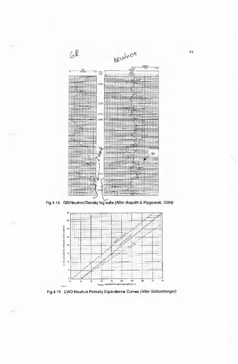
Fig 4.14 GR/Neutron/Density log suite (After Asquith & Krygowski, 2004)

Осэтчэ'. чрряи-nt Hi r:cs tone pcrosity (p )

Fig 4.15 LWD Neutron Porosity Equivalence Curves (After Schlumberger)

THE FORMATION DENSITY COMPENSATED (FDC) LOG

The FDC log records the bulk density (pb) of the formations surrounding the borehole. Fig 4.16

illustrates the principle of the tool which consists of a gamma ray source and two detectors

mounted on a pad. The pad is pressed against the borehole wall by a spring-loaded arm and

carries a plough which scrapes some of the mud cake to minimise its contribution to the bulk

density measurement. Since the measurement is made in contact with the borehole wall, any

loss of contact renders the log reading invalid over the interval where this occurs.

Fig 4.16 Diagrammatic illustration of the Formation Density Compensated (FDC) tool (After Schlumberger)

Gamma rays are beamed at the formations by the source. These enter the formations and

undergo multiple collisions with electrons in the rocks, as a result of which they lose energy and

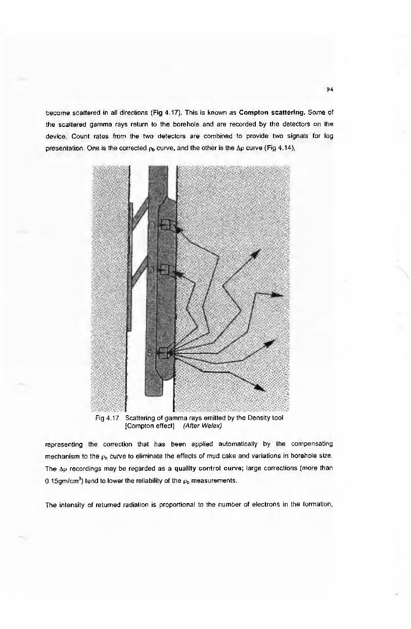
become scattered in all directions (Fig 4.17). This is known as Compton scattering. Some of

the scattered gamma rays return to the borehole and are recorded by the detectors on the

device. Count rates from the two detectors are combined to provide two signals for log

presentation. One is the corrected pb curve, and the other is the Ap curve (Fig 4.14),

*«V

• V

Fig 4.17 Scattering of gamma rays emitted by the Density tool [Compton effect] (After Welex)

representing the correction that has been applied automatically by the compensating

mechanism to the pb curve to eliminate the effects of mud cake and variations in borehole size.

The Др recordings may be regarded as a quality control curve; large corrections (more than

0-15gm/cm3) tend to lower the reliability of the pb measurements.

The intensity of returned radiation is proportional to the number of electrons in the formation,

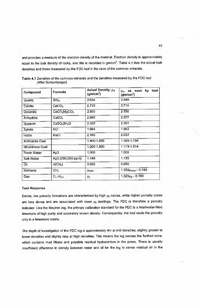
and provides a measure of the electron density of the material. Electron density is approximately

equal to the bulk density of rocks, and this is recorded in gm/cm3. Table 4.1 lists the actual bulk

densities and those measured by the FDC tool in the case of the common minerals.

Table 4.1 Densities of the common minerals and the densities measured by the FDC tool (After Schlumberger)

Compound Formula Actual Density, ph (gm/cm3)

pa, as seen by tool (gm/cm3)

Quartz S i02 2.654 2.648

Calcite СаСОз 2.710 2.710

Dolomite СаСОзМдСОз 2.850 2.850

Anhydrite CaS04 2.960 2.977

Gypsum CaS042H20 2.320 2.351

Sylvite KCI 1.984 1.863

Halite NaCI 2.165 2.032

Anthracite Coal 1.400-1.800 1.355-1.796

Bituminous Coal 1.200-1.500 1.173-1.514

Fresh Water H20 1.000 1.000

Salt Water H20 (200,000 ppm) 1.146 1.135

Oil n(CH2) 0.850 0.850

Methane

XО

Pmelh 1.335pmem- 0.188

Gas C i.iH « Pg 1.325Pg- 0.188

Tool Response

Dense, low porosity formations are characterized by high рь values, while higher porosity zones

are less dense and are associated with lower pb readings. The FDC is therefore a porosity

indicator. Like the Neutron log, the primary calibration standard for the FDC is a freshwater-filled

limestone of high purity and accurately known density. Consequently, the tool reads the porosity

only in a limestone matrix.

The depth of investigation of the FDC log is approximately 4in at mid densities, slightly greater at

lower densities and slightly less at high densities. This means the log senses the flushed zone,

which contains mud filtrate and possible residual hydrocarbon in the pores. There is usually

insufficient difference in density between water and oil for the log to sense residual oil in the

flushed zone. On the other hand, it can readily sense residual gas, especially if porosity is high

and gas pressure is low. The effect of gas is a lowering of the рь reading, resulting in a

spuriously large computed porosity.

The vertical resolution of the tool, if run slowly, is approximately 2ft. Formation density is

averaged over that interval.

Log Presentation

As mentioned before, the FDC is normally run simultaneously with the CNL and the curves are

recorded in tracks 2 and 3 (Fig 4.14). The FDC is recorded as a solid curve and calibrated in

gm/cm3, each division representing 0.05 gm/cm3.

А Др correction curve is also recorded in track 3, with zero at the centre and ± 0.25gm/cm3 at the

extremes. The Др curve indicates the correction that has been applied to the рь curve to

compensate the measurements for the effects of the mudcake and variations in the size of the

borehole. It should be considered as a quality control curve and it is not necessary to add its

readings to or subtract them from the pb curve. In a smooth hole the Др curve should be close to

the zero line, a little to the right for normal (non-barite) mud, and to the left for heavily loaded

barite mud. When mudcake or hole rugosity is encountered, the Др correction will increase. As

long as Др is less than 0.15gm/cm3, the correction is adequate and the pb curve is reliable.

Above O.I5gm/cm3 the correction is likely to be inadequate and the pb curve in error.

Evaluation of Porosity {aD) From The FDC Log

For a formation with a matrix density pma, containing a fluid of density pf, the pb reading given by

the FDC log represents the summation of the matrix and fluid responses. The matrix response is

given by the amount of matrix (1 - Ф) multiplied bypma, and the fluid contribution equals the

amount of fluid (Ф) multiplied by pf. Thus:

Pb = (1 - Ф)рта + $pf 4-2

Solving for Ф:

V'­' /

VФ0 - (p т а ~ рь)/(р та ” Pf)

Typical matrix densities (gm/cm3) are:

2.65 for sands, sandstones and quartzites

2.68 for calcareous sands or sandy limestones

2.71 for limestones

2.87 for dolomites

Porosity (Ф0) may be derived from Fig 4.18, which provides a graphical solution to equation 4.3.

Bulk density is entered on the bottom scale and porosity is read on the vertical scale for

appropriate values of pma and pf. Ф0 represents the total porosity in clean (shale-free), water

bearing and gas-free porous and permeable zones, provided the lithology is known.

Fig 4.18 Porosity derivation from the Density log (After Schlumberger)

THE LITHO-DENSITY LOG

The Litho-Density Tool (LDT) was introduced in the 1980s and has now replaced the FDC log. In

addition to the pb measurement, it provides a photoelectric absorption curve, Pe, which

measures the average atomic number of a given formation and is therefore a good indicator of

the rock matrix. It is particularly useful in complex lithology interpretation.

The source-detector arrangement of the LDT is basically the same as that of the FDC but the

operation is different. With the LDT, pb and Pe measurements are made by energy selection of

the gamma rays that reach the long-spacing detector. This is shown in Fig 4.19 which is a plot of

the number of gamma rays reaching the detector, as a function of their energy, for three

formations having the same bulk density but different volumetric absorption indices, U,

designated low, medium and high.

A C O U N T RA TE

Fig 4.19

The bulk density measurement is made by registering only those gamma rays that fall in the

high-energy region designated H in Fig 4.19. In this range only scattering of the gamma rays

takes place and the number of gamma rays, represented by the area under the curve, depends

on electron density only. Conversion of count rate to bulk density and correction for mudcake

and rugosity are carried out in the same manner as for the FDC log. Statistical fluctuations in

computed density, however, are reduced by a factor of about 2, to the range 0.01 to 0.02g/cm3,

by utilization of more efficient detectors.

LDT photoelectric and bulk density detection windows (After Schlumberger)

R eg ion o f p h o to e le c tric e ffec t and C o m p to n sca tte rin g .

L o w UM edium U

H igh U

[ j t

R eg ion of C o m p to n s c a tte r in g . _ L j

' of

The photoelectric absorption curve is produced by the interaction of gamma rays and electrons.

In this context gamma rays are considered as photons and the absorption of a photon by an

electron generates a photoelectron. At high energy levels, represented by window H in Fig 4.19,

the gamma rays undergo Compton scattering and are not absorbed. After several collisions, the

gamma rays lose sufficient energy to be absorbed by electrons. The photoelectric measurement

is made by registering those gamma rays that fall in window L, positioned at very low energy. In

this region gamma rays undergo photoelectric absorption the rate of which depends on the

product of the absorption coefficient per electron. Pe, and the electron density, p0. The count rate

at window L is related to a photoelectric absorption index or capture cross section, U, given by:

U - Pe Pe 4.4

Table 4.2 lists the Peand U values for the compounds that are commonly encountered in the

interpretation of the LDT log.

Table 4.2 Pe and U values for various compounds (After Schlumberger) оЛ г

Compound Formula peActual Density, pb (gm/cm3)

pa, as seen by tool (gm/cm3)

и

Quartz S i02 1.806 2.654 2.650 4.79

Calcite СаСОз 5.084 2.710 2.708 13.77

Dolomite CaMg (СОз)г 3.142 2.850 2.864 9.00

Anhydrite Ca S04 5.055 2.960 2.956 14.95

Gypsum Ca S04 2H20 3.420 2.320 2.372 8.11

Sylvite KCI 8.510 1.984 1.916 16.30

Halite NaCI 4.650 2.165 2.074 9.65

Siderite FeC03 14.690 3.890 3.810 55.90

Pyrite FeS2 17.000 5.000 4.990 82.10

Barite BaS04 266.800 4.500 4.011 1070.00

Water (fresh) H20 0.358 1.000 1.00 0.40

Water (120,000 ppm) H20 0.807 1.086 1.185 0.96

OilCH16 0.119 0.850 0.948 0.11

CH2 0.125 0.850 0.970 0.12

Gas

Xи

0.095 Pg 1-25Pg 0.11 9pg

Log Presentation

LDT measurements are recorded across tracks 2 and 3 as shown Fig 4.20. The bit size, GR and

caliper logs are displayed in track 1. Normally, however, the LDT is run simultaneously and

recorded with the CNL and NGS logs. Fig 4.21 shows a modern NGS/LDT/CNL log suite. The

current practice is to present the bit size, NGS and caliper measurements in track 1 and display

the LDT/CNL data in tracks 2 and 3. The greater variations in the Pe values of the common

reservoir rocks makes the LDT log a useful aid in their identification.

__CR_______.. .

- - -

PEP- ДГ “ DIUIO

r«t--- - Mb ----045ЮЮ6

— П-L-

■ J T T "-I'7' - T ; - -JL

v-

\“ 7 ------- ------- -i- > ;—t

t -: - -

r i ---------- -_V -LШ

-------4-* .- -----

~r— -------t ...— -

tr : : . ■ .Г -

i ___ ;_________

_____ _____

---------

. 1

/­- i —J .. ------------------

4.20 LDT log presentation (After Asquith & Krygowsky, 2004)

Fig 4.21 An NGS/LDT/CNL log suite

Heavy Mineral Identification

The LDT log is particularly useful in heavy mineral identification. Table 4.3 lists the pb and Pe

values of some of the more common heavy minerals.

Table 4.3 P0 and pb values of some heavy minerals

h

Mineral Pb Pe

Zircon 4.39 69

Siderite 3.89 14.7

Barite 4.10 267

Haematite 5.15 21

Magnetite 5.08 22

The photoelectric absorption index has a better resolution than the Density log as shown in Fig

4.22. Though the Density-Neutron combination does not show any obvious change in lithology,

the Pe curve indicates clearly the presence of a different mineral (Zone A). The zone is a

dolomite-limestone mixture with a siderite streak. The detection of heavy mineral streaks is

particularly useful in well-to-well correlation.

---- —* H— . ,

- . !•r .* LД ^ — —Г-

.w - M ♦4— ■pr ■' : ---

I--: —r—<i

■ 1—-}—I-m ---— 4jИ н■ 1

= Йj

-- i-J-U-l1-!-■• 1-r;.i..Pp t—v ..ML

-- 1—H-* ’- t“ tr:

Fig 4.22 Comparison of the LDT and FDC-CNL response to a heavy mineral (After Schlumberger)

A

This sensitivity to high Pe minerals is a drawback when drilling with barite-weighted muds. Even

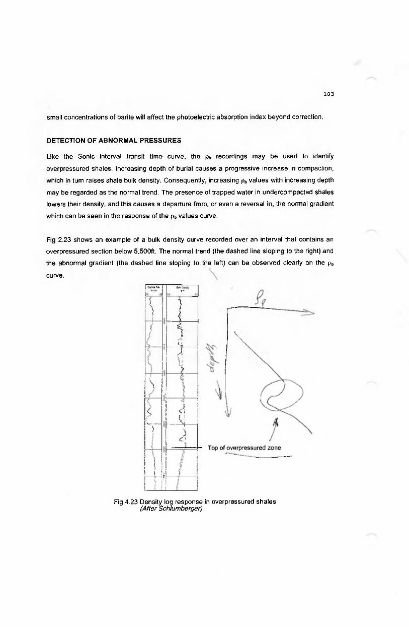
small concentrations of barite will affect the photoelectric absorption index beyond correction.

DETECTION OF ABNO RM AL PRESSURES

Like the Sonic interval transit time curve, the pb recordings may be used to identify

overpressured shales. Increasing depth of burial causes a progressive increase in compaction,

which in turn raises shale bulk density. Consequently, increasing pb values with increasing depth

may be regarded as the normal trend. The presence of trapped water in undercompacted shales

lowers their density, and this causes a departure from, or even a reversal in, the normal gradient

which can be seen in the response of the pb values curve.

Fig 2.23 shows an example of a bulk density curve recorded over an interval that contains an

overpressured section below 5,500ft. The normal trend (the dashed line sloping to the right) and

the abnormal gradient (the dashed line sloping to the left) can be observed clearly on the pb

curve.

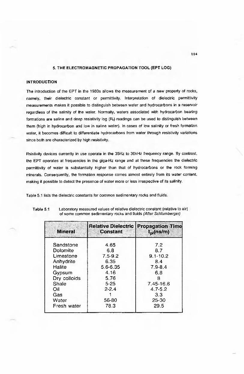
5. THE ELECTROM AGNETIC PROPAGATION TOOL (EPT LOG)

INTRODUCTION

The introduction of the EPT in the 1980s allows the measurement of a new property of rocks,

namely, their dielectric constant or permittivity. Interpretation of dielectric permittivity

measurements makes it possible to distinguish between water and hydrocarbons in a reservoir

regardless of the salinity of the water. Normally, waters associated with hydrocarbon bearing

formations are saline and deep resistivity log (Rt) readings can be used to distinguish between

them (high in hydrocarbon and low in saline water). In cases of low salinity or fresh formation

water, it becomes difficult to differentiate hydrocarbons from water through resistivity variations

since both are characterized by high resistivity.

Rsistivity devices currently in use operate in the 35Hz to 30kHz frequency range. By contrast,

the EPT operates at frequencies in the giga-Hz range and at these frequencies the dielectric

permittivity of water is substantially higher than that of hydrocarbons or the rock forming

minerals. Consequently, the formation response comes almost entirely from its water content,

making it possible to detect the presence of water more or less irrespective of its salinity.

Table 5.1 lists the dielectric constants for common sedimentary rocks and fluids.

Table 5.1 Laboratory measured values of relative dielectric constant (relative to air) of some common sedimentary rocks and fluids (After Schlumberger)

MineralRelative Dielectric

Constant». . • * . v -w ■ >.

Propagation Time tp,(ns/m)

Sandstone 4.65 7.2Dolomite 6.8 8.7Limestone 7.5-92 9.1-10.2Anhydrite 6.35 8.4Halite 5.6-6.35 7.9-8.4Gypsum 4.16 6.8Dry colloids 5.76 8Shale 5-25 7.45-16.6Oil 2-2.4 4.7-5.2Gas 1 3.3Water 56-80 25-30Fresh water 78.3 29.5

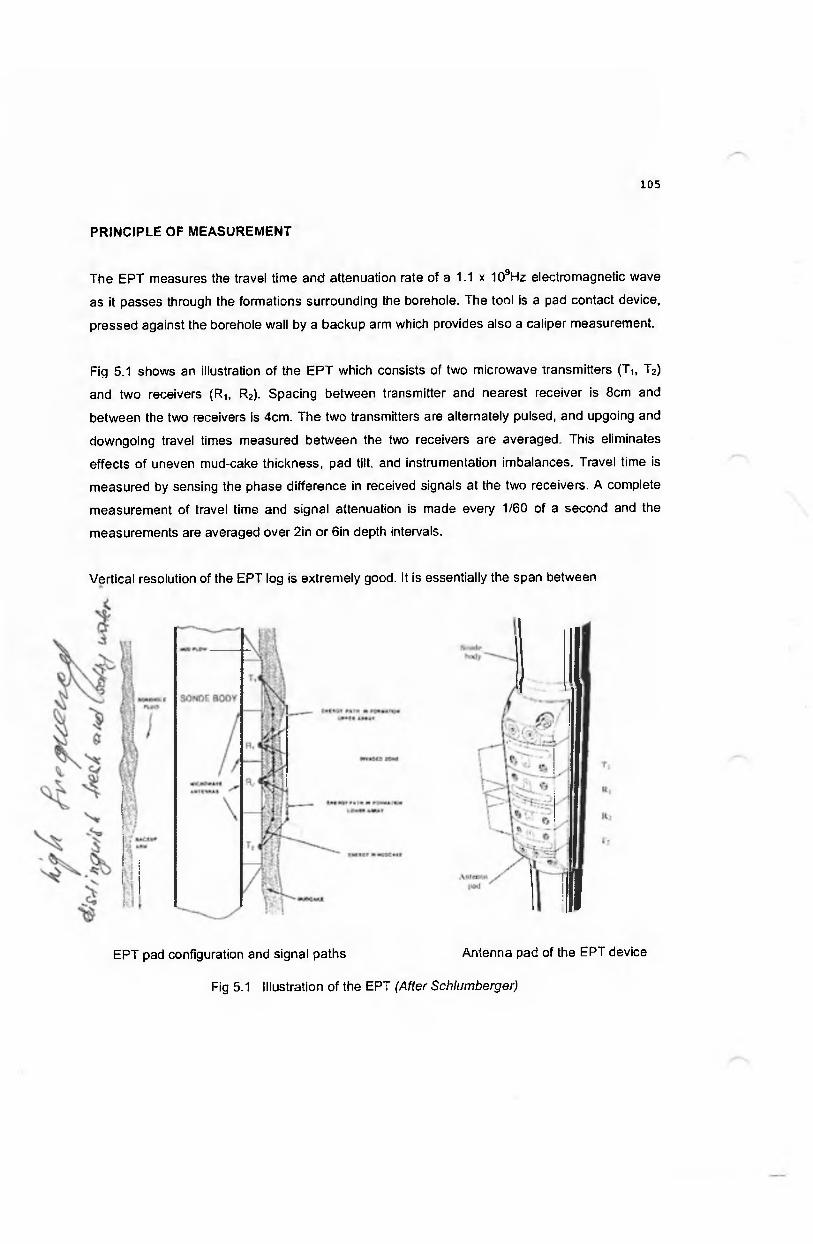
PRINCIPLE OF MEASUREMENT

The EPT measures the travel time and attenuation rate of a 1.1 x 109Hz electromagnetic wave

as it passes through the formations surrounding the borehole. The tool is a pad contact device,

pressed against the borehole wall by a backup arm which provides also a caliper measurement.

Fig 5.1 shows an illustration of the EPT which consists of two microwave transmitters (T1t T2)

and two receivers (Ri, R2). Spacing between transmitter and nearest receiver is 8cm and

between the two receivers is 4cm. The two transmitters are alternately pulsed, and upgoing and

downgoing travel times measured between the two receivers are averaged. This eliminates

effects of uneven mud-саке thickness, pad tilt, and instrumentation imbalances. Travel time is

measured by sensing the phase difference in received signals at the two receivers. A complete

measurement of travel time and signal attenuation is made every 1/60 of a second and the

measurements are averaged over 2in or 6in depth intervals.

Vertical resolution of the EPT log is extremely good. It is essentially the span between

EPT pad configuration and signal paths Antenna pad of the EPT device

receivers, which is about 2in. Depth of penetration is quite small, varying from about 1in in

low-resistivity formations to about 6in in high resistivity zones. The radius of investigation of the

tool is thus limited to the flushed zone, and the lower limit of formation resistivity for proper tool

operation is approximately 0.3 ohm-m2/m.

Borehole size and mudcake thicknesses of up to 3/8in have no effect on the EPT measurements

as long as the pad makes good contact with the borehole wall. Travel time increases with

increasing mudcake thicknesses and at 3/4in the response comes almost entirely from the

mudcake. Hole rugosity is also a problem, since it reduces the degree of contact between the

pad and the borehole wall.

A later adaptation of the EPT enables the device to provides more reliable measurements of

travel time and signal attenuation rates in rugse sections and in the presence of thick mudcakes.

Known as the ADEPT E lectrom agnetic Propagation Tool, it uses more advanced antennas

that reduce signal scatter and interaction with other electrical phenomena.

LOG PRESENTATION

A typical log presentation is shown in Fig 5.2. A GR log and standard caliper (hole diameter, HD)

are recorded in track 1, the electromagnetic wave attenuation (EATT), measured in decibels/m

and propagation time (TPL), measured in nanosec/m, are presented in tracks 2 and 3. There is

also a small arm caliper measurement (SA) displayed in track 2. This provides a more sensitive

caliper measurement than the standard device and is a better indicator of borehole rugosity.

INTERPRETATION

As mentioned above, at frequencies in the gigaHz range, the dielectric permittivity of water is

substantially higher than that of hydrocarbons or the rock forming minerals. Since substances

with high dielectric permittivity or constant are characterized aslo by high electromagnetic wave

propagation time, EPT measurement in clean formations is affected primarily by the water-filled

porosity. This contrasts with porosity values derived from radioactive logs, which respond to total

porosity, and consequently a combination of LDT, CNL and EPT data makes it possible to

№•к*®

GR (GAPlj . 100 200

GR(6APi)5 ■ - ' Too ' ■ ■ .

HO (in.)^ - - - - - -

______ р ш° 1

- У . r v > - . . • •

•: 'fc A rr (d 8 /m ) ,

y^tfSCw^.1 - r. : • »■/•* .__rw- (ns/m).' _ _ .

5 ~ i__~ ... ,.

Fig 5.2 EPT log presentation (After Schlumberger)

distinguish between oil, gas and water in reservoirs independent of formation water

characteristics.

It should be emphasised, however, that due to the shallow depth of investigation of the tool

(1-6in), it can usually be assumed that only the flushed zone is influencing the measurement and

the formation water is represented by the mud filtrate.

Quick look Hydrocarbon Indication

A combination of EPT, resistivity and radioactive porosity log data may be used in qualitative

evaluation of hydrocarbon bearing zones. Fig 5.3 shows schematically how the combination of

Induction, Density, Neutron, and EPT logs distinguish between fresh water, salt water, oil, and

gas. Resistivity distinguishes fresh water from salt water, whereas the other curves do not. EPT

distinguishes oil from fresh water while the other curves show only slight change. Finally, EPT

and Neutron-Density together distinguish gas from oil, while the resistivity is not definitive.

Since the EPT log responds primarily to water-filled porosity in clean formations, a qualitative

comparison of EPT porosity with the total porosity derived from the Density, Neutron or the

Sonic tools allows a quick-look identification of hydrocarbons in the flushed zone.

Fig 5.4 is an example comparing the Sonic porosity (SPHI) with the EPT porosity (EMCP). The

porosity curves are displayed in tracks 2 and 3 and the computed gamma ray (CGR) and total

gamma ray (SGR) from the NGS survey are recorded in track 1. There is a change in lithology at

245m, with a limestone above this depth and a sandstone with calcareous cement below. The

limestone and the lower section of the sandstone are water bearing, and the hydrocarbon

content of the upper section o f the sand is clearly indicated by the separation of the two porosity

curves. The original oil/water contact is at 267m, while the present contact is at 262m.

Fig 5.3 Comparison of Resistivity, Neutron, Density and EPT log responses in hydrocarbon and water bearing zones (After Schlumberger)

Fig 5.4 Quick look identification of hydrocarbon bearing zones by comparing sonic and EPT porosities (After Schlumberger)

Generally, the EPT porosity will read the same as a nuclear or acoustic derived porosity in water

bearing zones, but in hydrocarbon bearing intervals the EPT porosity will be less than the total

porosity. In gas-bearing zones the separation between the Neutron porosity and the EPT

porosity will not be so apparent because of the effect of gas on the Neutron measurement.

An example of the application of the EPT to the identification of the hydrocarbon bearing section

in a reservoir containing fresh formation water is shown in Fig 5.5. The LLD and LLS curves read

high resitivities throughout the section and do not differentiate between hydrocarbon and fresh

water since both are poor conductors and exhibit high resistivity. However, when EPT porosity

( Ф е р т ) is compared with that derived from the Neutron-Density log combination (Фда). a

hydrocarbon/water contact is indicated at 6,850ft.

Hydrocarbon/water contact

Fig 5.5 Hydrocarbon detection in a fresh water bearing reservoir (After Schlumberger)

Conversion of EPT M easurem ents to Porosity (Ф ерт)

Travel time and signal attenuation recordings can be used to calculate Ферт and the procedures

are reviewed briefly below.

tpo method

The t ^ method is based on the principle that the travel time (tp0) of electromagnetic waves in a

clean, lossless (low attenuation), porous, water-bearing medium is the sum of two individual

responses, namely, that of the matrix (tpma) and that of the pore water (tpw), the time being

measured in nanosec/m (ns/m). The matrix response is given by the amount of matrix (1 - Ф)

multiplied by tpma, and the water contribution equals the amount of water (Ф) multiplied by tpw.

Thus:

tpo — {1 " Ф)1рта + 5.1

Solving for Ф:

Ф ё РТ — Opo " tpma)/(tpw" tpma) 5.2

tpo is related to the measured travel time (tpi, ns/m) and Ac (db/m), the attenuation of the medium

corrected for spreading loss:

For carbonates and clean sandstones, the attenuation is negligible so that tpo is the actual tpi

value read from the log.

Values o f tp™ for various rock matrices and of tp„ for fresh water are given in Table 5.1. Values of

the dielectric constant, e , relative to air = I, are also listed in Table 5.1. Propagation time in ns/m

is related to e by the simple relation:

Consequently, the measured travel time o f a medium is a strong function of its water content.

Actual porosity will be higher if the formation contains hydrocarbons, since ФЕрт derived from

equation 5.2 represents water-filled porosity only.

This is a simpler approach than the tpo method and is based on the relationship between the

actual measured propagation time, tpi, and Ф Е р т and tpw:

tpo = [tpi2 - (Ac2/3 6 0 4 )]1/2 5.3

tpl = (11.1f.r)1/2 5.4

tpi method

tpl (I “ Ф р-ПЭ ■*" tpw 5.5

Solving for Ф:

Ферт = {tPi - tpma)/(tpw “ tpma) 5.6

Ac m ethod

Ac, the attenuation of the medium corrected for spreading loss, is related to Aw> the attenuation

of the pore water, by the following relationship:

Ac - Ф ерт Aw

5.7

Solving for Ферт

Ферт = 5.8

Ферт values obtained by these methods may differ. No one of them may be claimed to be more

reliable than the other two, and the most consistent results are obtained in homogeneous, high

porosity formations.

Derivation of Sxo From The EPT Log

Ферт would be the true porosity if all pores were water filled. It approximates the water-filled

porosity in formations containing hydrocarbons since the tool does not distinguish between

hydrocarbons and the rock matrix; travel times in the two media are similar. Consequently, a

comparison between ФЕрТ and total porosity, generally obtained from Density-Neutron logs,

allows a quick-look determination of Sxo:

Sxo- Ф ерт/Ф 5.9

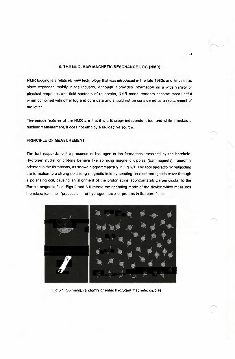
6. THE NUCLEAR MAGNETIC RESONANCE LOG (NMR)

NMR logging is a relatively new technology that was introduced in the late 1980s and its use has

since expanded rapidly in the industry. Although it provides information on a wide variety of

physical properties and fluid contents of reservoirs, NMR measurements become most useful

when combined with other log and core data and should not be considered as a replacement of

the latter.

The unique features of the NMR are that it is a lithology independent tool and while it makes a

nuclear measurement, it does not employ a radioactive source.

PRINCIPLE OF MEASUREMENT

The tool responds to the presence of hydrogen in the formations traversed by the borehole.

Hydrogen nuclei or protons behave like spinning magnetic dipoles (bar magnets), randomly

oriented in the formations, as shown diagrammatically in Fig 6.1. The tool operates by subjecting

the formation to a strong polarising magnetic field by sending an electromagnetic wave through

a polarising coil, causing an alignment of the proton spins approximately perpendicular to the

Earth's magnetic field. Figs 2 and 3 illustrate the operating mode of the device which measures

the relaxation time - ‘precession’ - of hydrogen nuclei or protons in the pore fluids.

Fig 6.1 Spinning, randomly oriented hydrogen magnetic dipoles

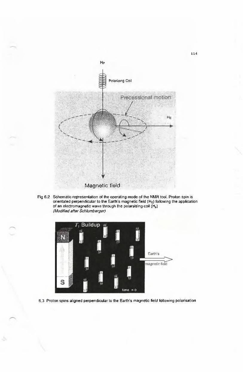
т

M agnetic field

Polarizing Coil

Fig 6.2 Schematic representation of the operating mode of the NMR tool. Proton spin isorientated perpendicular to the Earth’s magnetic field (HE) following the application of an electromagnetic wave through the polarsising coil (Hp)(Modified after Schlumberger)

6.3 Proton spins aligned perpendicular to the Earth's magnetic field following polarisation

The time taken for full polarisation is called 7, and for this to occur the polarising field must be

applied for a period about five times 7i. The electromagnetic wave is then turned off, allowing

the protons to 'relax' or 'precess' back to their original orientation. As the protons relax they emit

a weak signal which is detected by an antenna. The relaxation time T2 is measured and

recorded by the device. The antenna acts as both transmitter and receiver.

TOOL RESPONSE

There are three components to T2, referred to as surface, bulk and diffusion relaxations. The

dominance of any one component as the main relaxation process is governed by the pore fluids

and wettability of the reservoir.

Surface relaxation is the dominant process in totally water saturated pores. In this case collision

with grain surfaces is the most important factor in determining T2. In small pores collision with

grain surfaces is frequent, resulting in rapid relaxation. There are fewer collisions in larger pores

and the protons take longer to relax. Pore size distribution therefore affects relaxation times, as

shown diagrammatically in Fig 6.4. Consequently, there is a direct relationship between the

amplitude of the Тг measurement and porosity and permeability. Short T2 times generally

A totally water bearing pore

Fig 6.4 Effect of

Large pore ' '? 4 \

C'on

• Hydrogen prc:on rtec, msecCollisions with grain surfaces are more frequent in smaller pores, leading to shorter T2 times (After Schlumberger)

pore size on T2 in a totally water saturated reservoir

indicate small pores with low permeability, while longer T2 times indicate larger pores with higher

permeability.

Figs 6.5 and 6.6 show examples of the relationship between porosity and permeability and Гг-

The sandstone depicted in Fig 6.5 has a porosity of 20% and a permeability of 8 md. Fig 6.6

represents a sandstone with a similar porosity but a much higher permeability of 280 md.. The

latter is associated with a longer relaxation time on account of its higher permeability.

Fig 6.5 Effect of low permeability on relaxation time (After Schlumberger)

_ c. ctf О

(Л —

i

. ~ * s s

High permeability, producer

Porosity = 19.5% Permeability = 280 md

■ ' f : / Increasing relaxation time

о

\ . r $

Bulk relaxation is predominant in the non-wetting fluid phase in a reservoir and is controlled by

the physical properties of the fluid, such as its viscosity and density. The left diagram in Fig 6.7

shows a pore in an oil bearing, water wet reservoir. Being the non-wetting phase, the oil is not in

direct contact with pore walls. In this example the proton relaxation mechanism in the oil phase

is illustrated in the right diagram in Fig 6.7. Surface relaxation proceeds in the wetting water

phase.

{Thickness of the water film) ~ .

A water wet oil bearing pore Bulk relaxation in the non wetting oil phase

Fig 6.7 Illustration of bulk relaxation

Gas, oil and water exhibit significant molecular Diffusion induced relaxation. This is caused by

the molecules moving along gradients resulting from variations in the strength o f the magnetic

field produced by the polarizing coil (Fig 6.8).

/■"' - .-*4V

* > r *> . .

■ . - - ^ 4 , *

Fig 6.8 Illustration of diffusion relaxation

These three processes act in parallel and the overall T2 time is given by the following

relationship:

1/ 7*2 = 1/7surface + 1/7bulk + l/^diflusjon

INTERPRETATION

In conjunction with other log data, NMR measurements yield a wealth of information on rock and

fluid properties and these are discussed below.

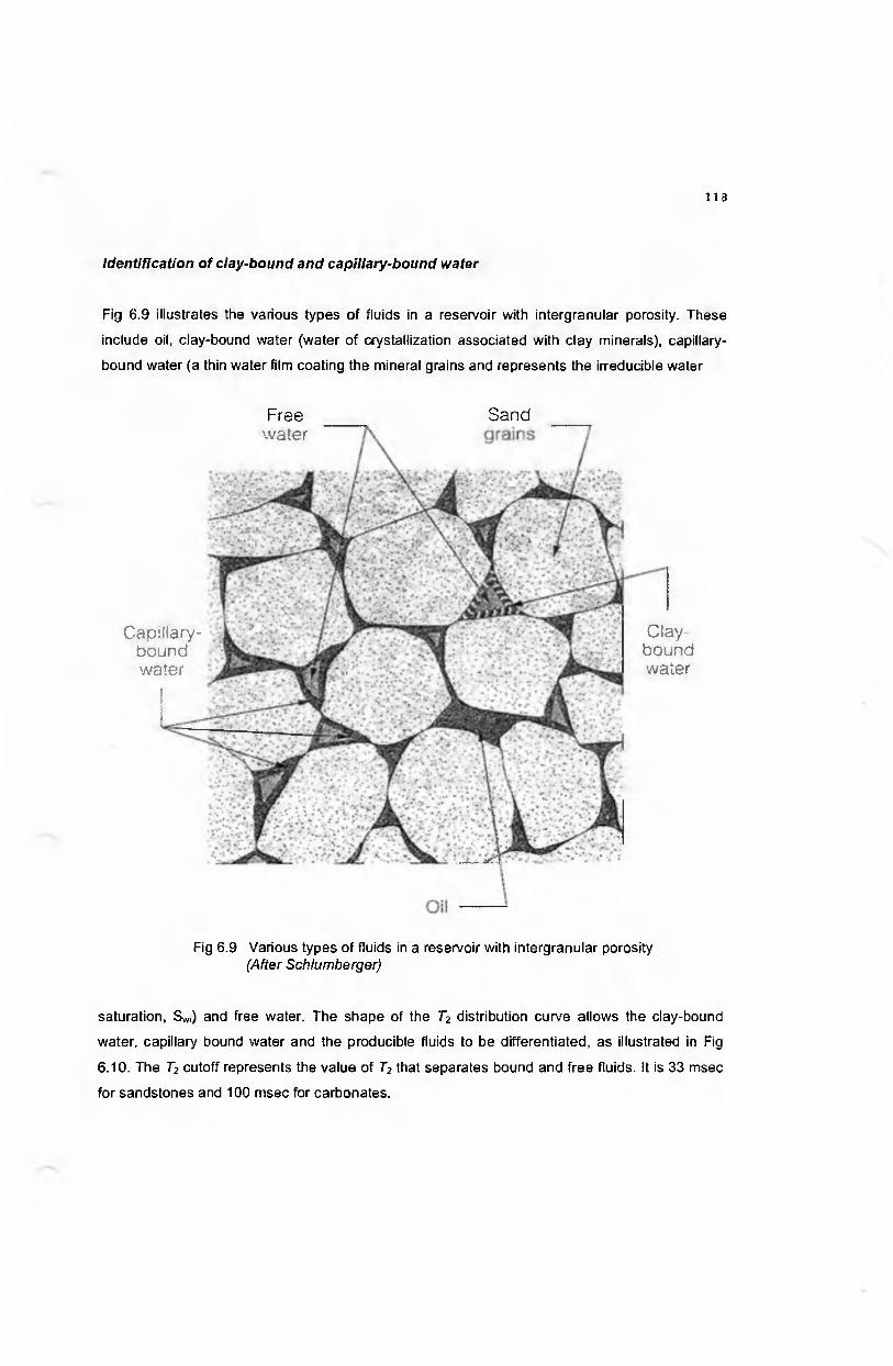
Identification of clay-bound and capillary-bound water

Fig 6.9 illustrates the various types of fluids in a reservoir with intergranular porosity. These

include oil, clay-bound water (water of crystallization associated with clay minerals), capillary-

bound water (a thin water film coating the mineral grains and represents the irreducible water

Clay-boundwater

Freewater

Capillary-boundwater

Sand

Fig 6.9 Various types of fluids in a reservoir with intergranular porosity (After Schlumberger)

saturation, Sw,) and free water. The shape of the T2 distribution curve allows the clay-bound

water, capillary bound water and the producible fluids to be differentiated, as illustrated in Fig

6.10. The T2 cutoff represents the value of T2 that separates bound and free fluids. It is 33 msec

for sandstones and 100 msec for carbonates.

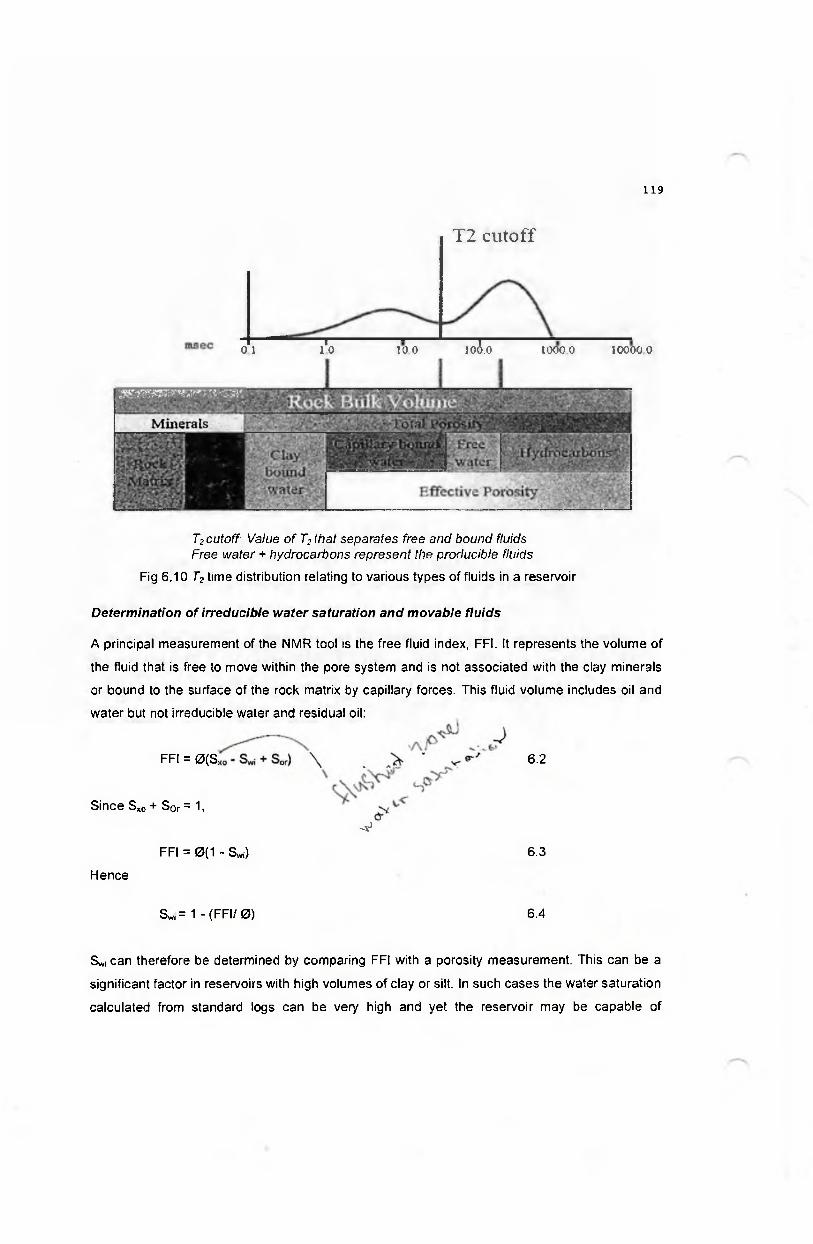
T2 cutoff

0 1 l'o 10 0 10^0 1000.0 10000 0

T2cutoff: Value o f T2that separates free and bound fluids Free water + hydrocarbons represent the producible fluids

Fig 6.10 T2 time distribution relating to various types of fluids in a reservoir

Determination of irreducible water saturation and movable fluids

A principal measurement of the NMR tool is the free fluid index, FFI. It represents the volume of

the fluid that is free to move within the pore system and is not associated with the clay minerals

or bound to the surface of the rock matrix by capillary forces. This fluid volume includes oil and

water but not irreducible water and residual oil:

Since S*0 + S0r = 1,

FFI = 0(S ;

-V

6.2

FFI = 0(1 - Swi) 6.3

Hence

Sw,= 1 - (FFI/ 0 ) 6.4

Swi can therefore be determined by comparing FFI with a porosity measurement. This can be a

significant factor in reservoirs with high volumes of clay or silt. In such cases the water saturation

calculated from standard logs can be very high and yet the reservoir may be capable of

producing dry oil. The reason for this anomaly is that the water is associated with the clay

minerals and is not free to move.

An example of an NMR log over a shaly sand interval with calcareous cement is presented in

Fig 6.11. The topmost section is associated with very high SWj values and very low FFI readings.

The latter indicate that the water is not free to move and therefore bound water.

Determ ination o f e ffective p o ro s ity

NMR measurements provide effective porosity values independent of lithology. This is useful in

complex lithology reservoirs and shaly sands where it is difficult to derive porosity from standard

logs. Examples of NMR derived porosity curves are shown in Figs 6.12 and 6.13.

P erm eability estim ation

As mentioned above, proton relaxation time (Г2) is related to pore size distribution and can be

used to estimate permeability. In granular reservoirs small pore sizes correspond generally to

lower permeabilities while higher permeabilities are associated with larger pore sizes. A variety

of methods are available to determine NMR permeability and the choice is governed by

operating company preference, reservoir conditions and service company. NMR derived

permeability curves are displayed in track 2 in Figs 6.11 and 6.12 and in many cases NMR

permeabilities are comparable with those from core measurements (Fig 6.11). It should be

noted, however, that the current methods resolve only matrix permeability and underestimate

the permeability of fractured formations. Isolated vuggy pores in carbonates also present a

problem.

The vugs often contain free fluids and are associated with high FFI values but their isolation

prevents them from contributing to permeability. Consequently, the NMR permeability in such

cases is an overestimation.

Pore size d is tribu tion

Since the proton relaxation time of a fluid within a single pore is proportional to the size of that

pore, as a first approximation, the distribution of T2 measurements within a reservoir reflects the

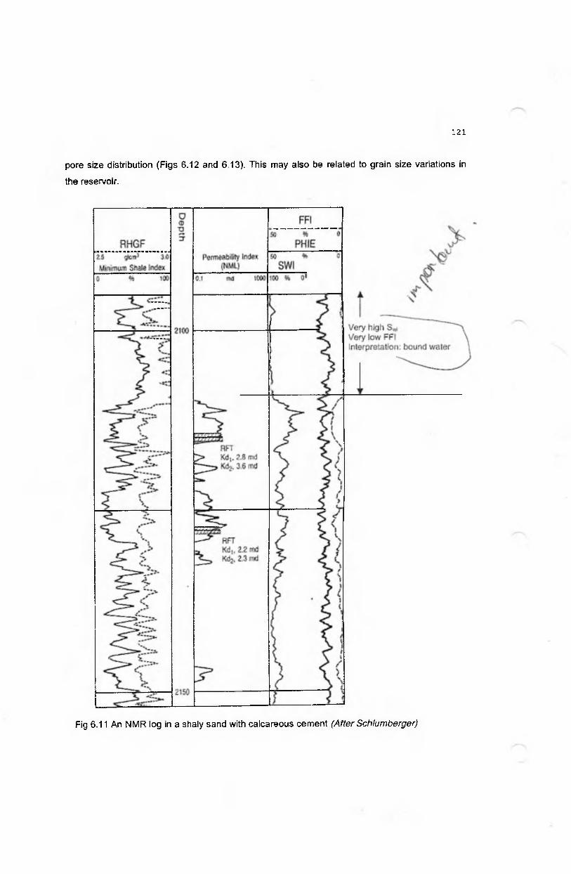
pore size distribution (Figs 6.12 and 6.13). This may also be related to grain size variations in

the reservoir.

H ydrocarbon detection

As shown in Table 6.1, reservoir fluids exhibit different polarization (Trf and relaxation times (T2).

These variations are used in MNR logging to detect hydrocarbons. Viscosity contrasts are

Table 6.1 NMR properties of reservoir properties (After Coates et al, 1999)

Reservo ir flu id T i{ msec) T2 (msec) V iscos ity (cp)

Brine 1 -500 1 -500 О Kj I о CO

Oil 3 ,000 -4 ,0 00 3 0 0 - 1,000 0 .2 - 1,000

Gas 4,000 - 5,000 3 0 -6 00.011 -0 .0 1 4

(methane)

particularly useful in identifying heavy oil and tar deposits. The NMR log responds to these

heavy substances as if they are solids - very little or no FFI is measured. However, for the direct

identification of medium to light oils and gas and determining their saturation without

incorporating data from conventional resistivity and porosity logs, specialised pulse sequences

are required.

Fig 6.12 shows an example of reservoir fluid identification by the NMR log.

COMMERCIALLY AVAILABLE TOOLS

The NMR is a highly versatile log with a wide range of applications. It works in the presence of

most drilling fluids with the exception of high salinity water based muds. Currently, there are two

commercial tools: the Combinable Magnetic Resonance (CMR) tool offered by Schlumberger

and the Magnetic Resonance Imaging Log (MRIL) available from Haliburton and Baker Hughes.

(Figs 6.13 and 6.14).

Irreducible water

Water

Zone

Free water

XX700

xxsoo

XX900

1 2Distribution

Borehole

CMRPermeability

0.1 md 1000

NeutronPorosity

DensityPorosity

0.3 3000

msec

Depth,ft

GammaRay

0 API 150

Fig 6.12 Formation fluid identification by the NMR log (After Schlumberger)

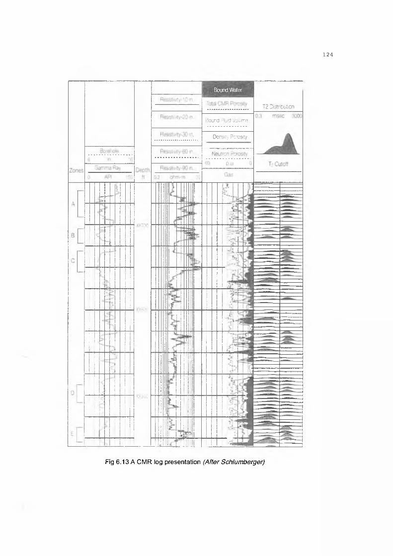
Bound Water

T2 Distribution

3ound Fiwd Vc'ume

Density Porosity

0 API 2СС

Perm eability (md)

Resistivity (ohm -m )

2000

2000 Pcrosity (% )

Fig 6.14 An MRIL presentation (After Baker Atlas)

7. PLATFORM EXPRESS (PEX)

PEX is a new log data acquisition technology, developed and introduced in thejmid-1990sjand

represents a major departure from conventional wireline logging tools. The system integrates

multiple functions into a single package or p la tform with the various sensors incorporated in the

same device rather than as a series of separate tools connected together in a string. The PEX

device is less than half the length and of a conventional trip le com bo which has been in use

since the mid-1980s.

Fig 7.1 provides a comparison between the lengths of a PEX device and the conventional triple

combo: the former is less than half the length and weight of the latter. A summary of the

'

■ i

90 ft {27 rpj

Fig 7.1 Comparison between the lengths of PEX and conventional triple combo (After Schlumberger)

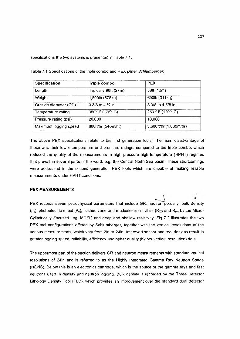
specifications the two systems is presented in Table 7.1.

Table 7.1 Specifications of the triple combo and PEX (After Schlumberger)

Specification Triple com bo PEX

Length Typically 90ft (27m) 38ft (12m)

Weight 1,5001b (675kg) 690lb (311kg)

Outside diameter (OD) 3 3/8 to 4 1/ 2 in 3 3/8 to 4 5/8 in

Temperature rating 350° F (175° C) 250° F (120° C)

Pressure rating (psi) 20,000 10,000

Maximum logging speed 800ft/hr (540m/hr) 3,600ft/hr (1,080m/hr)

The above PEX specifications relate to the first generation tools. The main disadvantage of

these was their lower temperature and pressure ratings, compared to the triple combo, which

reduced the quality of the measurements in high pressure high temperature (HPHT) regimes

that prevail in several parts of the word, e.g. the Central North Sea basin. These shortcomings

were addressed in the second generation PEX tools which are capable of making reliable

measurements under HPHT conditions.

PEX M EASUREM ENTS

PEX records seven petrophysical parameters that include GR, neutron porosity, bulk density

(pb), photoelectric effect (Pe), flushed zone and mudcake resistivities (Rxo and Rmc by the Micro-

Cylindrically Focused Log, MCFL) and deep and shallow resistivity. Fig 7.2 illustrates the two

PEX tool configurations offered by Schlumberger, together with the vertical resolutions of the

various measurements, which vary from 2in to 24in. Improved sensor and tool designs result in

greater logging speed, reliability, efficiency and better quality (higher vertical resolution) data.

The uppermost part of the section delivers GR and neutron measurements with standard vertical

resolutions of 24in and is referred to as the Highly Integrated Gamma Ray Neutron Sonde

(HGNS). Below this is an electronics cartridge, which is the source of the gamma rays and fast

neutrons used in density and neutron logging. Bulk density is recorded by the Three Detector

Lithology Density Tool (TLD), which provides an improvement over the standard dual detector

measurements. Other features of the TLD device include higher precision in denser formations

and less sensitivity to barite which results in better Pe measurements. The TLD tool and MCFL

are housed in the High Resolution Mechanical Sonde (HRMS) which also incorporates a caliper.

Hinge joints above and below the HRMS enable the tool to better negotiate borehole wall

irregularities (Fig 7.3). This improves pad contact and maintains density and Rxo log data quality

in washed out and rugose sections. Real time log quality control allows corrections to be made

to off-depth log readings caused by tool sticking. Fig 7.4a presents a standard GR-DLL-MSFL

showing off-depth readings resulting from tool sticking. In Fig 7.4b the ‘speed correcting’ of the

high resolution PEX data has removed the mis-match between the GR and resistivity curves.

Toolacceleration

Highly Integrated Gamma Ray ~

Neutron Sonde (HGN3)

GR 2 4 m

0 N 12 to 24 r\.

Bectronicscartridge

Hingejoint

t >b.Pe2. 8, 18 in R*o, Rrnc

High-ResofuuonMechanical

Scnde

Caliper

Hingejoint

High-Resoiution Azimuthal Laterolog

Sonde iHALS)—ti

*HALS

Я». Rf

Rt12

AIT Array induction Imager Tool

AIT

Fig 7.2 PEX tool configurations Vertical resolutions of each measurement are indicated (After Schlumberger)

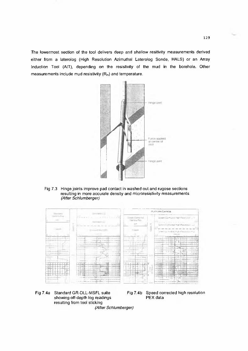
The lowermost section of the tool delivers deep and shallow resitivity measurements derived

either from a laterolog (High Resolution Azimuthal Laterolog Sonde, HALS) or an Array

Induction Tool (AIT), depending on the resistivity of the mud in the borehole. Other

measurements include mud resistivity (Rm) and temperature.

Fig 7.3 Hinge joints improve pad contact in washed out and rugose sections resulting in more accurate density and microresistivity measurements (After Schlumberger)

Pl a t f o r m Ex p r e s s

Speea-CofTftC!fc<l K»gh-Resn*u?ron lLS

SPCW ) COn*2Ct«4j H*jh-RsscM-on ILD

5pe®> l -Ctxfectod Htgh-PesoM wo RXO

7ТГ—

±—4-~fj—

Fig 7.4a Standard GR-DLL-MSFL suite showing off-depth log readings resulting from tool sticking

(After Schlumberger)

Fig 7.4b Speed corrected high resolution PEX data

ADVANTAGES

The high vertical resolution data produced by PEX logging are useful in the identification of thin

beds. In Fig 7.5 three 2-in tight streaks (seen also in the microresistivity log not shown here) are

detected by their high density log readings. These can act as vertical permeability barriers.

Fig 7.5 High resolution density measurements identify three 2-in tight streaks (seen also in the microresistivity log not shown here) which can act as vertical permeability barriers (After Schlumberger)

Due to higher speeds, PEX logging operation takes less time and the reduced weight and length

make the tool easier to handle. The savings in time are reflected in reduced rig and average

logging times, lowering the cost of data acquisition. Fig 7.6 shows rig time comparisons between

the conventional triple combo and PEX in land and offshore operations in Venezuela while Fig

7.7 provides the same illustrations in Saudi Arabia and Argentina.

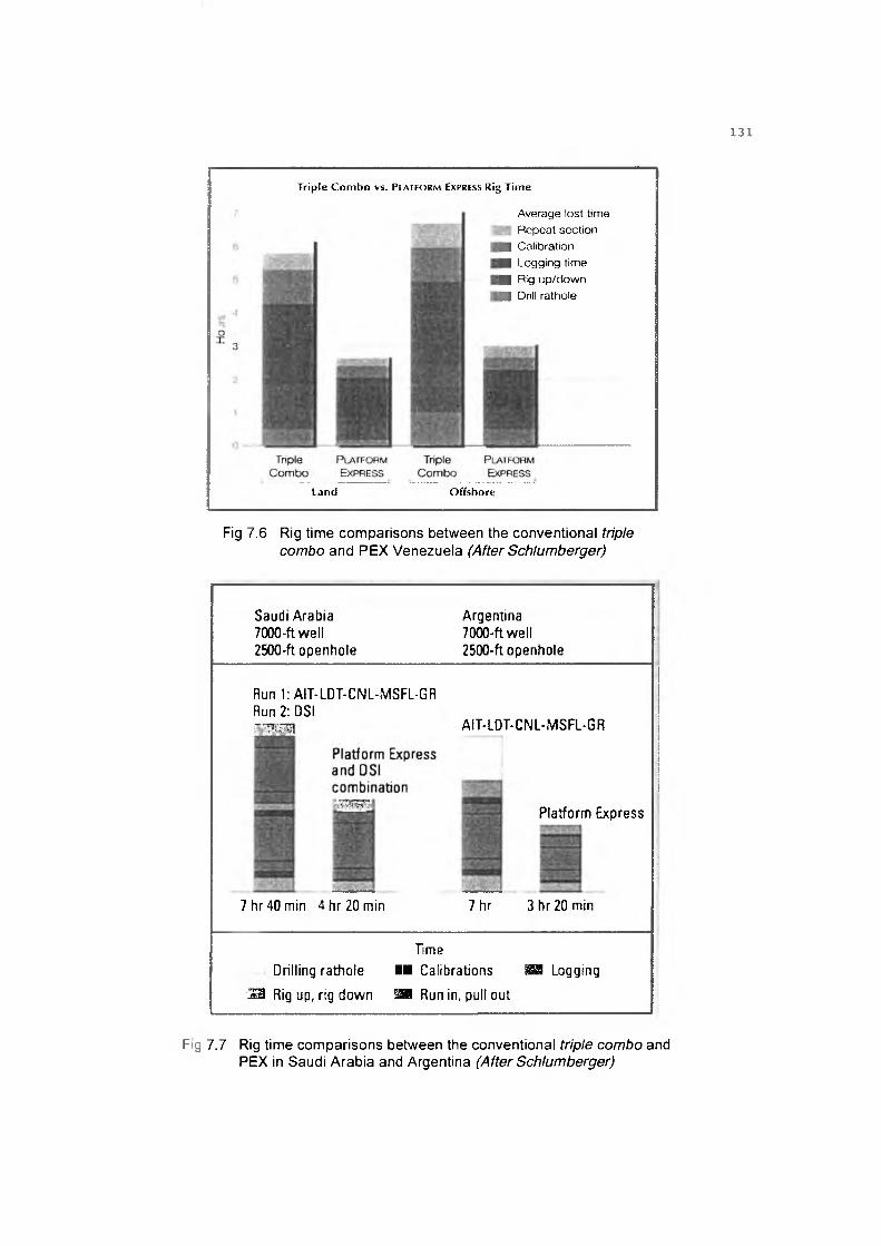
T r ip le C o m b o vs. P l a t f o r m E x p r e s s R ig T im e

Average lost time Repeat section

■ Calibration■ Logging time■ Rig up/down О Drill rathole

Land O ffs h o re

Fig 7.6 Rig time comparisons between the conventional triple combo and PEX Venezuela (After Schlumberger)

Saudi Arabia 7000-ft well 2500-ft openhole

Argentina 7000-ft well 2500-ft openhole

Run 1: AIT-LDT-CNL-MSFL-GR Run 2: DSI

AIT-LDT-CNL-MSFL-GR

Platform Express

7hr40m in 4 h r20m in 7 hr 3 h r20m in

TimeDrilling rathole ■■ Calibrations Ш Logging

'ЗЕЭ Rig up, rig down Шк Run in, pull out

Fig 7.7 Rig time comparisons between the conventional triple combo and PEX in Saudi Arabia and Argentina (After Schlumberger)

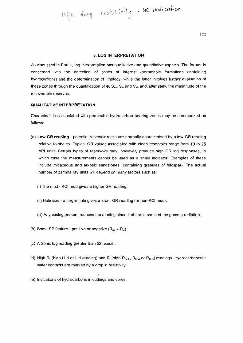
, v < './Л . . ЙС w*h©irh ;<]V

и

8. LOG INTERPRETATION

As discussed in Part 1, log interpretation has qualitative and quantitative aspects. The former is

concerned with the detection of zones of interest (permeable formations containing

hydrocarbons) and the determination of lithology, while the latter involves further evaluation of

these zones through the quantification of Ф, Sxo, Sw and VSh and, ultimately, the magnitude of the

recoverable reserves.

QUALITATIVE INTERPRETATION

Characteristics associated with permeable hydrocarbon bearing zones may be summarized as

follows:

(a) Low GR reading - potential reservoir rocks are normally characterised by a low GR reading

relative to shales. Typical GR values associated with clean reservoirs range from 10 to 25

API units..Certain types of reservoirs may, however, produce high GR log responses, in

which case the measurements cannot be used as a shale indicator. Examples of these

include micaceous and arkosic sandstones (containing granules of feldspar). The actual

number of gamma ray units will depend on many factors such as:

(i) The mud - KCI mud gives a higher GR reading:

(ii) Hole size - a larger hole gives a lower GR reading for non-KCI muds;

(iii) Any casing present reduces the reading since it absorbs some of the gamma radiation .

(b) Some SP feature - positive or negative (Rmf * Rw).

(c) A Sonic log reading greater than 52 (.isec/ft.

(d) High R, (high LLd or ILd reading) and R, (high R Sfl, R ilm or RLLS) readings. Hydrocarbon/salt

water contacts are marked by a drop in resistivity.

(e) Indications of hydrocarbons in cuttings and cores.

X '

v$

§

'I

4 G"4_X ^

v / \ \i' a

L- ч4

54

Lithology Determination and Gas Detection

Fig 8.1 is an illustrated presentation of the log values associated with the common lithologies

and fluids and Fig 8.2 shows the idealized GR-LDT-CNL log combination responses to the rock

types frequently encountered in oil and gas wells.

Fig 8.1 Log values to common lithologies and fluids (After Baker Hughes)

The GR-LDT-CNL combination gives a good lithological indication except in the presence of

gas. A tight, clean sandstone is associated with a pb reading of about 2.65gm/cm3 and a Фм of

- 4. The Фм curve is to the right of the pb curve, the separation between them being 2 -4 scale

divisions. Tight limestones are characterised by the pb overlying the Фм curve with the former

reading 2.7gm/cm3 and the latter zero porosity. In a tight dolomite Фм reads about + 4 and pb is

about 2.87gm/cm3. In this case, pb is deflected to the right of the Фм curve. Shales or mudstones

are associated with very high Фм values (up to 45 p.u. in some cases). Consequently, the Фм

curve moves to the left and crosses the pb curve. This cross-over is matched by a deflection to

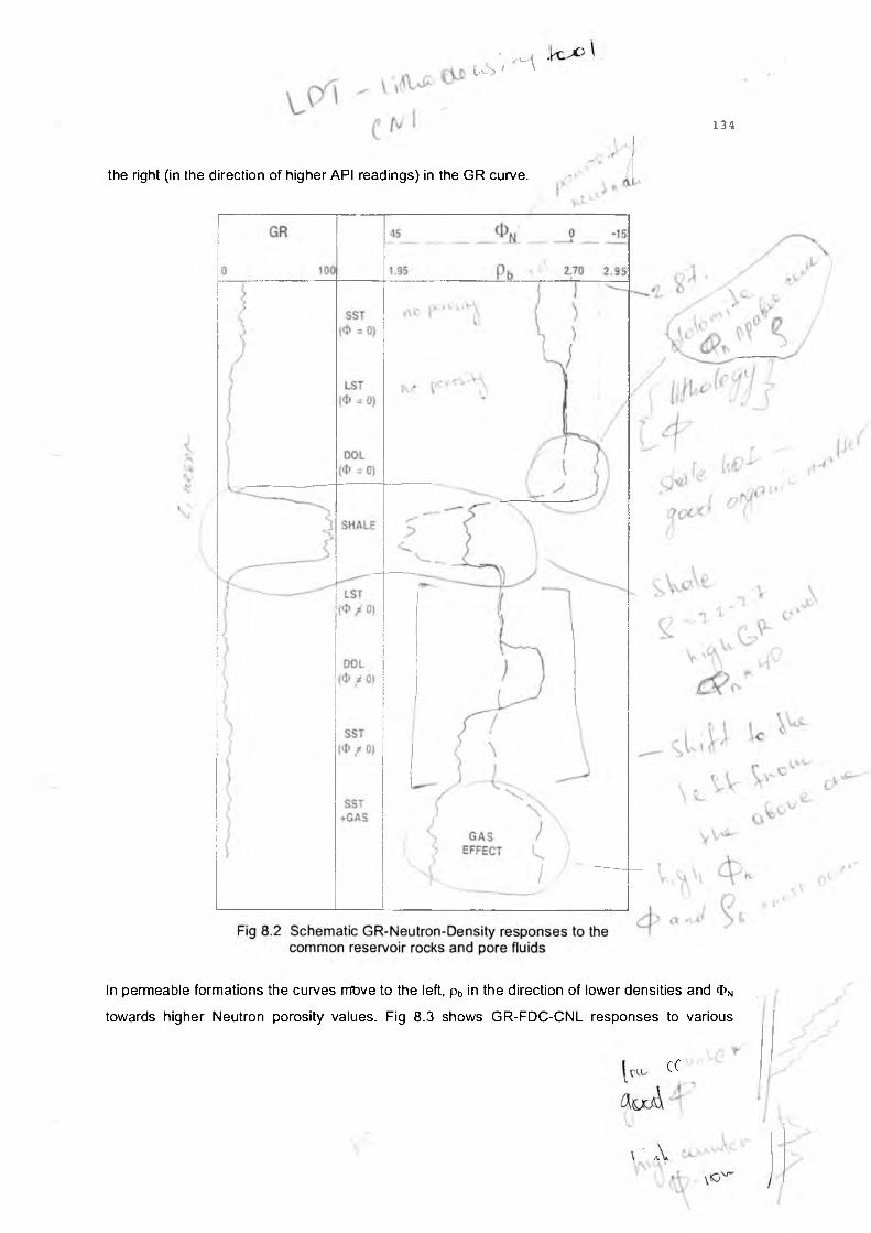
Сл-> ’/ М

the right (in the direction of higher API readings) in the GR curve.

In permeable formations the curves mtive to the left, pb in the direction of lower densities and <t>N

towards higher Neutron porosity values. Fig 8.3 shows GR-FDC-CNL responses to various

C°

lithologies and Figs 8.4 and 8.5 demonstrate their responses to carbonate-evaporite sequences.

If gas is present, the separation between the curves increases considerably; the Фм curve

moves to the right, in the direction of lower porosity (due to the low hydrogen index of gas), and

the pb curve slightly to the left, towards a somewhat lower density value. This is known as the

gas effect. Figs 8.6 is a general illustration of this phenomenon and Fig 8.7 shows a gas

bearing sandstone reservoir. A gas bearing limestone reservoir is shown in Fig 8.8.

A gas-bearing shaly sandstone may cause confusion. Since gas and shale have opposite effects

on the Neutron log, the influence on one may cancel that of the other, resulting in the elimination

of the gas effect on the Density-Neutron combination. However, a reference to the GR curve

should resolve such a situation.

Im proved Clay Mineral Identifica tion

In the discussion of the Natural Gamma Ray Spectrometry Tool (NGS), it was pointed out that

clay mineral identification on the basis of NGS data alone is not entirely free from ambiguity, and

that better results could be obtained by cross-plotting these data with photoelectric absorption

(Pe) measurements made by the LDT log.

Figs 8.9 and 8.10 present two charts established for the express purpose of combining Pe and

NGS data. The chart in Fig 8.9 is entered by plotting the potassium concentration against the

corresponding Pe value, while in the chart in Fig 8.10 the thorium/potassium ratio is computed

and crossplotted versus the Pe measurement. Agreement between the results of these two

crossplots improves confidence in the clay mineral determination. General areas rather than

unique clay mineral poles are indicated on the charts. This is due to the wide variations in clay

mineral composition which cause some scattering of the points at which the minerals plot.

WIRE LINE LOG CHARACTERISTICS OF POTENTIAL SOURCE ROCKS

Source rocks are organic rich clay or carbonate muds that in their natural setting have generated

and released sufficient hydrocarbons to form a commercial accumulation of oil and gas. They

can be of marine or lacustrine (fresh water) origin. To function as a source rock, the sediment

must contain a minimum of 1.5 - 2% by weight of organic matter.

They can be identified qualitatively by their GR, neutron, density, son ic and res is tiv ity log

responses which are briefly described below.

A

Л \

Top reservoir

GOC

owe

Fig 8.6 Identification of gas, oil and water by a Neutron-Density-resistivity combination (Shell publication, 1994)

Fig 8.8 Limestone interval showing gas effect (After Schlumberger)

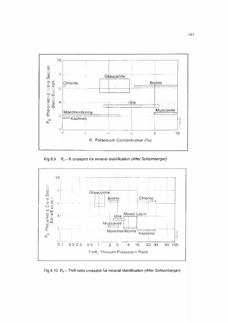
10

сОо0)00

со 2О g W шоCDО.'оо.с:CL

а>О.

озсо

О

G laucon ite

C hlorite B io tite

M ontm orillon ite

Kaolim te

llite

t

□M uscovite

<£>CO■£}c*J

2 4 6 8

K, Potassium C oncentra tion (% )

10

Fig 8.9 Pe - К crossplot for mineral identification (After Schlumberger)

10 i

cОоa>CO(Л с O 2о йо

CD

uu о 1_<DО) пзО СПо ’

0 L

CL

G laucon ite

B iotite Chlorite

IlliteM ixed Layer

M uscovite и -------p

M ontm orillon iteKaolin ite

00.1 0 .2 0 .3 0 .6 1 2 3 6 10 2 0 3 0

Th/K , Thorium -Potassium Ratio

60 100

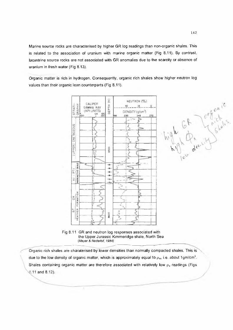
Marine source rocks are characterised by higher GR log readings than non-organic shales. This

is related to the association of uranium with marine organic matter (Fig 8.11). By contrast,

lacustrine source rocks are not associated with GR anomalies due to the scarcity or absence of

uranium in fresh water (Fig 8.13).

Organic matter is rich in hydrogen. Consequently, organic rich shales show higher neutron log

values than their organic lean counterparts (Fig 8.11).

Fig 8.11 GR and neutron log responses associated with the Upper Jurassic Kimmeridge shale, North Sea (Meyer & Nederlof, 1984)

Organic rich shales are charaterised by lower densities than normally compacted shales. This is

due to the low density of organic matter, which is approximately equal to pw, i.e. about 1 gm/cm3.

Shales containing organic matter are therefore associated with relatively low pb readings (Figs

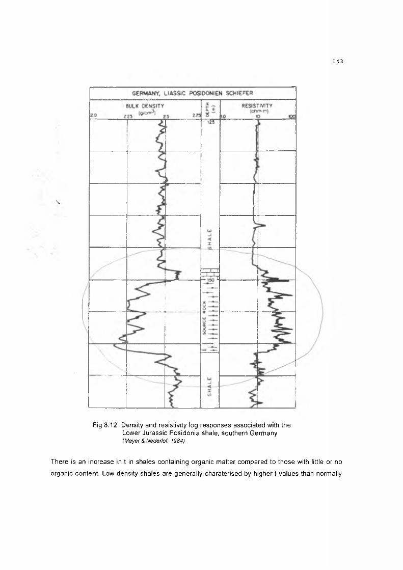
Fig 8.12 Density and resistivity log responses associated with the Lower Jurassic Posidonia shale, southern Germany (Meyer & Nederiof, 1984)

There is an increase in t in shales containing organic matter compared to those with little or no

organic content. Low density shales are generally charaterised by higher t values than normally

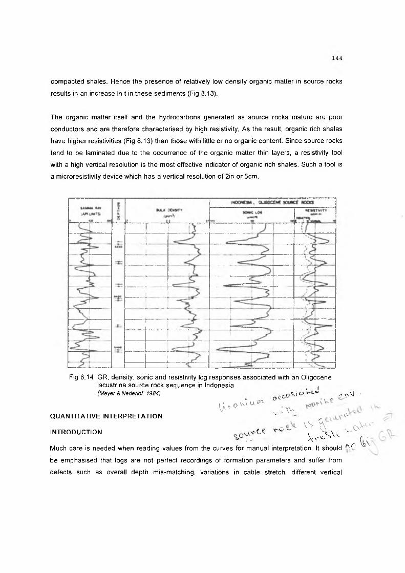
compacted shales. Hence the presence of relatively low density organic matter in source rocks

results in an increase in t in these sediments (Fig 8.13).

The organic matter itself and the hydrocarbons generated as source rocks mature are poor

conductors and are therefore characterised by high resistivity. As the result, organic rich shales

have higher resistivities (Fig 8.13) than those with little or no organic content. Since source rocks

tend to be laminated due to the occurrence of the organic matter thin layers, a resistivity tool

with a high vertical resolution is the most effective indicator of organic rich shales. Such a tool is

a microresistivity device which has a vertical resolution of 2in or 5cm.

Fig 8.14 GR, density, sonic and resistivity log responses associated with an Oligocene lacustrine source rock sequence in Indonesia _ ,(Meyer & Nederlof, 1934)

QUANTITATIVE INTERPRETATION

INTRODUCTION

. . А X й -

\JU o V vV U » ~л \|

^ A V - ^ Vv

v>

О У*

a c\Much care is needed when reading values from the curves for manual interpretation. It should r

be emphasised that logs are not perfect recordings of formation parameters and suffer from

defects such as overall depth mis-matching, variations in cable stretch, different vertical

resolutions of different tools and the effect of statistical variations on the radioactive

measurements. There are also problems caused by poor borehole wall conditions.

Depth mis-matching can result in one logging run being at a different depth from another, a

common cause of which is cable stretching. The cable stretches under its own weight as well as

that of the logging tool. As the tool is pulled up the borehole, the length of cable is reduced,

resulting in a progressive decrease in the amount of stretch. This causes the depth-mismatch to

change in the course of the logging operation.

Combining several tools on the same run results in the measure points of the various curves not

being at the same level - some measurements may be memorised so that they can all be

recorded at the same depth. Another factor is the vertical resolutions of the various tools which

vary from 2in to 4ft. Consequently, thin beds can appear as only small changes in one log while

on curves produced by a tool with a better vertical resolution the same bed may appear as a

much larger deflection. In order to minimise these problems, it is recommended that when taking

readings from the logs, zones at least 2m (6ft) thick should be chosen, preferably where the

curves show relatively constant values. An eyeball average should be taken over the selected

interval.

Large washouts and borehole wall rugosity can affect the data quality by keeping the tools away

from the formation. The pad contact devices such as the Density and microresistivity logs are

affected the most. In large washouts, the pad loses contact with the borehole wall and its

readings become invalid, since they represent mud rather than formation parameters. The Sonic

log measurements may be affected by cycle skipping and the CNL may also read too high due

to a large contribution from the mud.

Sticking is also a problem and distorts the thickness of the section. It can be detected from the

tension curve and stationary readings on the non-radioactive logs. It should be noted that the

sticking may occur at different depths for the different curves because of the depth difference

between measure points.

It should be noted that logs are not the only source of information from a well. There is also a

litholog, a mud log, perhaps some core data with measured helium porosities and permeabilities

and side wall sample descriptions. The litholog is very useful since resolves the ambiguities that

sometimes arise in log interpretation.

The interpretation procedures presented here constitute what is known as the 'quick-look'

method, which is adequate for rapid well-site evaluation. Provided the corrections are properly

applied and the interpretation is carefully made, porosities can be expected to be accurate to ±2

units and water saturations to ± 0.10 in an uncomplicated reservoir.

OBJECTIVES

As stated above, the object of quantitative interpretation is to determine Ф, Ф, Sxo, Sw and Vsh.

Determination of Sw is particularly important, since it leads to a value for hydrocarbon saturation

(Sh) in the uninvaded zone:

Sh = 1 "Sw 8.1

Since Sw represents the fraction of the pore space filled by water, it follows that the porosity

fraction occupied by hydrocarbons is:

Ф(1 - Sw) 8.2

Expression 8.2 is an important factor in the estimation of the total volume of hydrocarbons

present in a given reservoir

Sw is derived from the Archie equation, a relationship developed in the 1930s by G.E. Archie,

and published formally in 1942 (see below). Porosity is one of the essential parameters in the

Archie equation, and must therefore be determined as accurately as possible. Knowledge of Vsh

is also important, since if it exceeds 15-20%, then the Sw value derived from the Archie equation

is unreliable.

Porosity may be derived from any one of the porosity logs (Sonic, Neutron or Density), as

demonstrated previously. However, by crossplotting information from two porosity logs, more

reliable values of Ф can be obtained. Crossplotting provides also a resolution of lithology for

mixtures of up to two minerals.

The steps involved in quantitative log interpretation are described below and summarised in the

flow chart presented in Fig 8.14.

POROSITY AND LITHOLOGY DETERMINATION BY CROSSPLOTTING

The porosity logs afford four possible crossplots:

Neutron-Density

Sonic-Neutron

Sonic-Density

P e"Pb

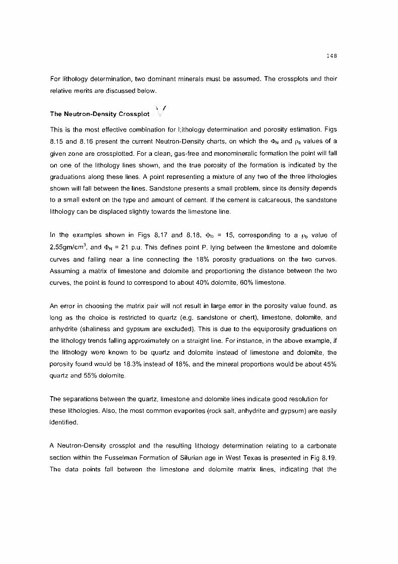
For lithology determination, two dominant minerals must be assumed. The crossplots and their

relative merits are discussed below.

' /The Neutron-Density C rossplot

This is the most effective combination for l;ithology determination and porosity estimation. Figs

8.15 and 8.16 present the current Neutron-Density charts, on which the On and pb values of a

given zone are crossplotted. For a clean, gas-free and monomineralic formation the point will fall

on one of the lithology lines shown, and the true porosity of the formation is indicated by the

graduations along these lines. A point representing a mixture of any two of the three lithologies

shown will fall between the lines. Sandstone presents a small problem, since its density depends

to a small extent on the type and amount of cement. If the cement is calcareous, the sandstone

lithology can be displaced slightly towards the limestone line.

In the examples shown in Figs 8.17 and 8.18, Ф0 = 15, corresponding to a pb value of

2.55gm/cm3, and Фм = 21 p.u. This defines point P, lying between the limestone and dolomite

curves and falling near a line connecting the 18% porosity graduations on the two curves.

Assuming a matrix of limestone and dolomite and proportioning the distance between the two

curves, the point is found to correspond to about 40% dolomite, 60% limestone.

An error in choosing the matrix pair will not result in large error in the porosity value found, as

long as the choice is restricted to quartz (e.g. sandstone or chert), limestone, dolomite, and

anhydrite (shaliness and gypsum are excluded). This is due to the equiporosity graduations on

the lithology trends falling approximately on a straight line. For instance, in the above example, if

the lithology were known to be quartz and dolomite instead of limestone and dolomite, the

porosity found would be 18.3% instead of 18%, and the mineral proportions would be about 45%

quartz and 55% dolomite.

The separations between the quartz, limestone and dolomite lines indicate good resolution for

these lithologies. Also, the most common evaporites (rock salt, anhydrite and gypsum) are easily

identified.

A Neutron-Density crossplot and the resulting lithology determination relating to a carbonate

section within the Fusselman Formation of Silurian age in West Texas is presented in Fig 8.19.

The data points fall between the limestone and dolomite matrix lines, indicating that the

formation is a mixed carbonate unit.

The chart includes also a provision for gas correction (top left-hand corner of Fig 8.15). In the

presence of gas, <J>N is lowered, and consequently gas-bearing zones tend to plot above the

Porosity and Lithology Determination IromFormation Density Log and CNL' Compensated Neutron LogFor CHL iocs felcre !93o 01 taDH?c NPHl

Porosity and Ltthoiogy Determination fromFormation Density Log and CNL‘ Compensated Neutron Log-V CfcL iOijs fcefcrj 1386, or а-ик-d fiPHi

**!• ЗСиСЫЙЧС *lt

Mud filtrate concentration < 100,000 ppm Mud filtrate concentration > 100,000 ppm

Fig 8.15 FDC-CNL cross plot charts (After Schlumberger)

Porosity and L:thj:ijiyy Determination (т,гп Liiho-Densily' Leg and CNL" Compensated Neutron Log

Porosity and Litho'ogy Determination trcrr[jtho-Density’ Log and CNL' Compensated Neutron Log

CfIL vlir.es ih ti -93? :гэе)и) TJJPrt

1 КО o'sw. С... о par . , 1ЛЛ*Чв\«(1.П C..«rsw*«e,

X* / }* ■ У

Л ■у

- . i . ■ KPу

j \ j/ ' .. : . \ X . _ > * *• У; У

. . . ; . У5!* jj

X ■ У ' ' у ' : ./ У • * i

У У 1 1

Mud filtrate concentration < 100,000 ppm Mud filtrate concentration > 100,000 ppm

Fig 8.16 LDT-CNL cross plot charts (After Schlumberger)

sandstone matrix line. Porosity can be corrected for the effect of gas by projecting the point,

parallel with the gas correction arrow, onto the appropriate matrix line as shown in Fig 8.20. A

Neutron-Density crossplot of several hundred data points from a Palaeocene age sand-shale-

p c n l (L im estone)

Fig 8.17 Porosity and lithology from determination FDC-CNL crossplot (After Schlumberger)

40

30

$ 20

10

- 1 0

]

1 / £

k £

Ъ / , /, К ' $ /

<$> / ! /

У Ж ь У л /

s > / ^ 4 1 л»/ .'■•О0

О\o

\

а /У

CJ ■у/

0 10 20 30 40

c>cnl (Limestone)

Fig 8.18 Porosity and lithology determination from the the LDT-CNL crossplot (After Schlumberger)

с /и ? / '- / t s

/ n d e sp cw e /a n '/ '

P - f I I K o t С

к

si

-A :- , .

SP-GR-DIL-SFL-LDT-CNL suite over the interval evaluated

Fig 8.19 A Neutron-Density crossplot and the resulting lithology determination, Fusselman Formation carbonates, West Texas (After Asquith & Krygowsky, 2004)

YY\Vl ( ( A .

tuff (lithified volcanic ash) sequence in a Northern North Sea well is presented in Fig 8.21.

<>n----- •­Fig 8.20 Hydrocarbon correction (After Schlumberger)

Fig 8.21 8Neutron-Density analysis of the Palaeocene section from a well in the Northern North Sea

Key to numbered clusters:

1, 2 & 5 - claystone, shale and minor tuff 3 - gas bearing sand 4 - Massive tuff 6 - oil bearing sand 7 - water bearing sand(After Hatton et at, 1992)

Variations in lithology and fluid content allow four clusters to be identified. The oil and water

bearing sands (cluster 6 & 7) appear to be relatively clean while the scatter of points falling

between the sandstone and dolomite matrix lines are shaly. The presence of gas in the sands

represented by the points in cluster 3 causes them to plot above the sandstone trend.

The Sonic-Neutron crossplot

This crossplot is also a good indicator of porosity and lithology. Fig 8.22 shows the

Sonic-Neutron crossplot charts relating to pre-1986 (NPHI) and post-1986 (TNPH) CNL logs.

The charts are entered by the t and <&N readings of a given zone. As with the Density-Neutron

plots, resolution between quartz, limestone and dolomite lithologies is good and the equiporosity

graduations on the 3 matrix trends fall approximately on a straight line. Porosity determination is

therefore largely independent of lithology.

Porosity and Lithology Determ ination from Sonic Log and CNL' Com pensated Neutron LogFo: CNL tngs neJore 19Я6. cr iSDf fril rjf-Hl

Porosiry and Lithology Determ ination from Sonic Log and CNL* Compensated Neutron Logfur CM logs alter 1986 !ab"iad >4?H

!. - 1 SO ..-икУП; С, - 0 ppm

I * /

/I

V // /■ , /

/ /j

4 ' /

/ / л f л9/ !

,/ r/ j / . ! ■J, "

У

Fig 8.22 Sonic-CNL cross plot charts (After Schlumberger)

However, there is no provision for gas correction, and this crossplot should not be used in

gas-bearing formations.

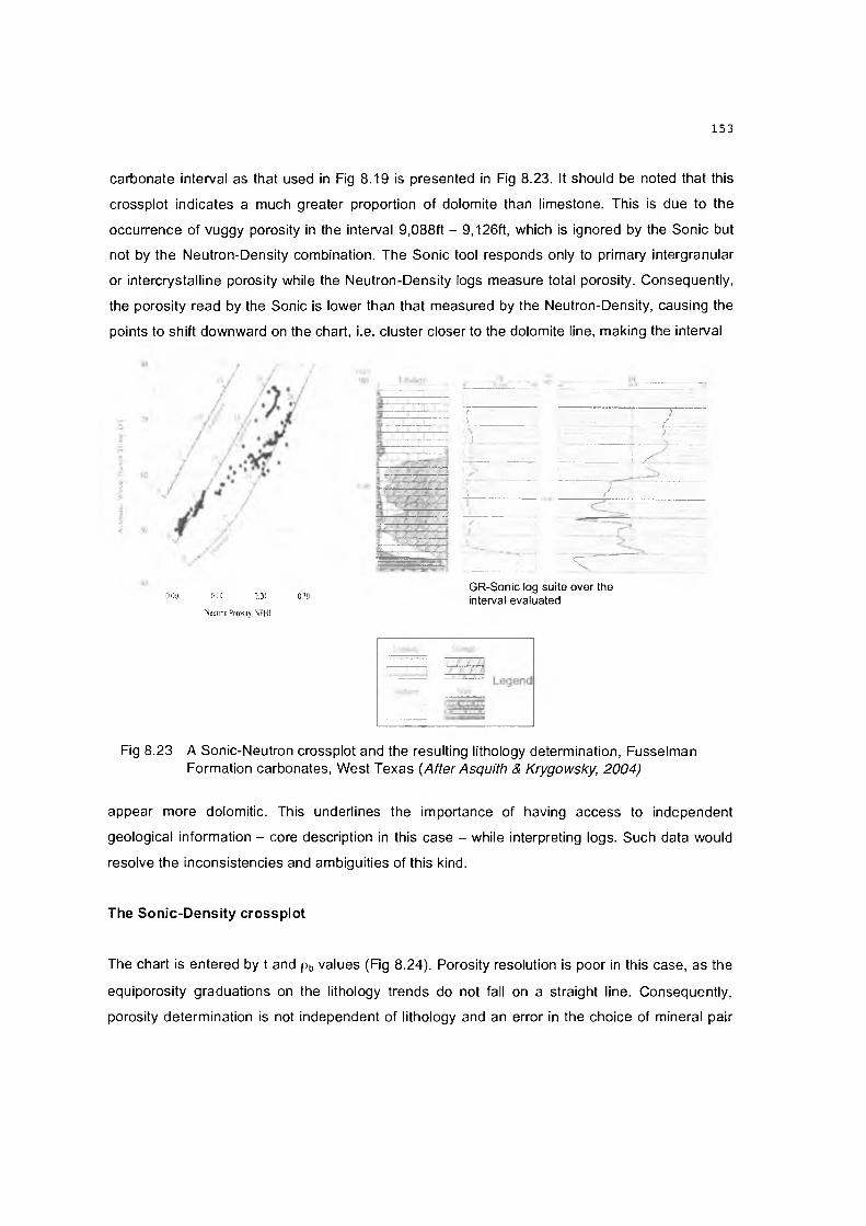
carbonate interval as that used in Fig 8.19 is presented in Fig 8.23. It should be noted that this

crossplot indicates a much greater proportion of dolomite than limestone. This is due to the

occurrence of vuggy porosity in the interval 9,088ft - 9,126ft, which is ignored by the Sonic but

not by the Neutron-Density combination. The Sonic tool responds only to primary intergranular

or intercrystalline porosity while the Neutron-Density logs measure total porosity. Consequently,

the porosity read by the Sonic is lower than that measured by the Neutron-Density, causing the

points to shift downward on the chart, i.e. cluster closer to the dolomite line, making the interval

0.00 0II) 0.20 0.30Neutron Pnrositv. N'P HI

(■ J . ) '' /

: / r ■• .

i f ' ::• ■ /

ЯGR-Sonic log suite over the interval evaluated

Fig 8.23 A Sonic-Neutron crossplot and the resulting lithology determination, Fusselman Formation carbonates, West Texas {After Asquith & Krygowsky, 2004)

appear more dolomitic. This underlines the importance of having access to independent

geological information - core description in this case - while interpreting logs. Such data would

resolve the inconsistencies and ambiguities of this kind.

The Sonic-Density crossplot

The chart is entered by t and pb values (Fig 8.24). Porosity resolution is poor in this case, as the

equiporosity graduations on the lithology trends do not fall on a straight line. Consequently,

porosity determination is not independent of lithology and an error in the choice of mineral pair

from the quartz-limestone-dolomite group can result in appreciable error in porosity estimation.

Lithology resolution is poor since the matrix lines are closely spaced, making it difficult to

differentiate between the minerals. The crossplot does, however, distinguish effectively between

the common evaporite minerals. As seen on the chart, good resolution is achieved for salt,

gypsum and anhydrite, since these mineral poles are widely separated.

Lithology Identification fromFormation Density Log and Sonic Log (E

If = 169 usee/ft; p, = 1.0

■*0 50 ftO 70 80 ЭД 100 110 120

1. sonic transit time (usec/fi)

Fig 8.24 Sonic- Density cross plot chart (After Schlumberger)

Fig 8.25 illustrates a Sonic-Density crossplot of the Fusselman Formation. The lithology of the

interval 9,088ft - 9,126ft, characterized by vuggy porosity, is now shown as limestone.

Underestimation of the porosity by the Sonic in the presence of vugs causes the points to shift

leftward on the chart and cluster around the limestone line.

The inconsistencies in lithology determination from the three crossplot techniques in relation to

interval 9,088ft - 9,126ft are in themselves significant: they indicate that the section has vuggy

porosity. Had all the porosity been primary intergranular or intercrystalline, the crossplots would

indicate similar lithology.

It should therefore be noted that lithology determinations that involve the Sonic log may be

unreliable if the interval in question has vuggy porosity.

2.20

3.00

4 0 50 60 70

Acoustic W ave Travel Time, DT

80

F E E TM D Lithology

Dokffiiiii

, t U A

Shale

Ш22ЕВ1

Legend

Fig 8.25 A Sonic-Density crossplot and the resulting lithology determination, Fusselman Formation carbonates, West Texas {After Asquith & Krygowsky, 2004)

The Pe - pb crossplot

Fig 8.26 presents the Ре-рь crossplot charts which are entered by the Pe and pb readings of a

given zone. A clean, gas-free and monomineralic zone will plot on one of the matrix lines

provided it is one of the lithologies shown on the chart and its porosity is indicated by the

graduations on the lines. A clean mixture of any two of the three minerals shown will fall

between the matrix lines and, assuming two dominant minerals, the relative amounts of these

may be estimated by proportioning the distance between the curves. As in the Density-Neutron

crossplot, the wide spacing between the matrix lines allows good lithology resolution.

Porosity may be determined by interpolating between the equiporosity lines joining the stems

representing the dominant lithologies assumed. However, the like Sonic-Density crossplot, the

equiporosity graduations on the lithology trends do not fall on a straight line and consequently

porosity determination is not independent of lithology; an appreciable error in porosity

determination will result from an incorrect choice of mineral pair. Also, there is no provision for

gas correction.

Porosity and Lithology Determination from Litho-Density* Log

Porosity and Lithology Determination from Litho-Density' Log

t'tniv u

1U

у■it:

I?

Mud filtrate concentration < 100,000 ppm Mud filtrate concentration > 100,000 ppm

Fig 8.26 LDT crossplot charts (After Schlumberger)

The advantages and limitations of the crossplot techniques outlined above are reviewed in Table

8.1. The Neutron-Density combination is the most effective and the most commonly used

crossplot.

Table 8.1 Relative merits of the various crossplot techniques

Crossplot Advantages Limitations

Neutron-Density Good resolution of lithology

Porosity determination independent of lithology

Provision for gas correction

Large holes and borehole wall rugosity may render the Density log data invalid

Density measurements affected by heavy drilling muds

Sonic-Neutron Good resolution of lithology

Porosity determination independent of lithology

Less sensitive to poor borehole conditions

The Sonic under-reads porosity when vugs are present

No provision for gas correction

Sonic-Density Effective in evaporite mineral identification

Poor resolution of lithology

Porosity determination not independent of lithology

No provision for gas correctionP e "P b Good resolution of lithology

Both measurements made by the same logging tool

Porosity determination not independent of lithology

No provision for gas correction

Vsh Determination

There are many different ways of determining Vstl in a shaly formation. The most rapid and

popular method is by the use of the GR curve, as demonstrated earlier. The equation used is:

Vsh — (GRzone " GRclean)/(GRshale " GRclean) 8.3

Graphical methods are also used commonly. These involve cross-plotting readings from two

porosity logs on a chart on which three components or points - the rock matrix, shale and fluid

(usually water) - must be identified (Fig 8.27):

Matrix - denoted by M and defined as all grains or crystals, no shale, no porosity and no

fluid.

Shale - designated S and defined as all shale, no matrix and no fluid.

Fluid - called F and defined as all fluid (100% porosity, no matrix and no shale.

Porosity increases along the line MF from 0 at M to 100% at F. Shale content, Vsh, increases

from 0 at M to 100% at S. The lines MF and MS are divided into 10 equal parts, each division

representing an increase of 10% in porosity and Vsh respectively. Fig 8.27 illustrates a Neutron-

Density crossplot chart constructed for a sandstone reservoir with a matrix density of

2.65gm/cm3.

Fig 8.27 Vsh and porosity determination in a shaly sand (After Schlumberger)

The matrix point coordinates in this case are therefore 2.65 and 0. The coordinates of the fluid

point are 1 (density of fresh water) and 100 neutron porosity units (<I>n )- The shale point has the

coordinates pbshaie and <&Nshaie, obtained from a shale interval associated with the reservoir.

The clean zones in this example will fall on MF (clean trend). Shaly zones plot below MF and

point A in Fig 8.27 represents such a case. Its shale content can be estimated by projecting the

point parallel with MF onto MS and its shale corrected porosity by projecting it parallel with MS

onto MF, as demonstrated in Fig 8.28.

In practice, formations with pb values of less than 2.00 gm/cm3 and <J>N readings of greater than

1 .2

1.4

1.6

1.8

6 b 2

2.2

2 .4

2.6

2.8

/ /

i/Vater

C o

(?m<

n d itic

a =*

>ns:

2.6580,4?

/

@sh

£?w

2.45

£\C)\ \ 60,­

// ,j / 7

<p<?°

40 j

/

^ 7 У

1

/4 / /

- Vl 7-7

/

Matri>

7Z /

// "'Shak

Sf

оM

&

\Js^[Vlo)

'<5 1969 Sc I

i__

____

__

O’ _I

erger

О 10 20 30 40 50 60 70 80 90 100

о N

Fig 8.28 Determining Vsh and shale corrected porosity (After Schlumberger)

50 PUs are rare and only the bottom left quadrant of the crossplot is relevant in practice. Manual

crossplotting can be undertaken by using the charts supplied by the service companies and the

following procedure outlines the Neutron-Density method (Fig 8.29):

(1). Plot the shale point on the Neutron-Density crossplot chart. The values for the shale point,

Pbshaie and 0 NShaie. can be obtained from the log by finding a neighbouring shale bed. If the

shale is within the reservoir, it is advisable to select maxima on the curves, since such beds

Fresh water, liquid-filled holes (p, = 1.0)

2.0

2.1

2.2

2 3

§ 2 .4>41ЛсВ•о

^ 2 .5эое?

2 6

W f R i x 7

2.8

2 .9

О 10 20 30 40

OeNLcor. neutron porosity index fp.u.j (apparent limestone porosity)

Fig 8.29 Neutron-Density cross plot constructed for porosity and Vsh determination in a shaly sand (Modified from Schlumberger)

are likely to contain some silt.

(2) Straighten the curved, low porosity end of the sandstone lithology trend and establish a

matrix point M as shown in Fig 8.29. Shaly zones such that represented by A plot below the

sandstone matrix line.

(3) Draw equiporosity lines parallel to the zero porosity line M-S.

(4) Divide M-S into ten equal parts and draw lines upwards parallel to the matrix line. These are

equi-shale fraction lines.

(5) For each point plotted, the shale fraction Vsh and Ф can now be estimated from this grid. The

shaly sand represented by point A in Fig 8.29 has а Фм reading of 16 PUs and a pb value of

2.38gm/cm3. The true porosity (corrected for the effect of shale) is found by projecting A

parallel to the equiporosity lines onto the matrix line established in (2) above, and amounts

to 13%. The shale fraction in this zone is determined by projecting A parallel to the

equi-shale lines on to the M-S line, giving a Vsh of about 20%.

(6) The case of a calcareous cemented sandstone is illustrated in Fig 8.30. The crossplot points

from such a reservoir fall below the sandstone matrix line due to the presence of the calcite

cement which causes them to shift towards the limestone lithology trend. The matrix trend in

this case is established by drawing a line originating at the zero porosity point and passing

through the plots closest to the sandstone line. The porosity graduations on the matrix trend

are determined by the intersections with lines joining equiporosity points between the

sandstone and limestone lines.

F re sh w a le r, liq u id - f ille d h o le s (p f = 1 .0 )

n e u tro n p o ro s ity m ci^x (p .u .) (a p p a re n t lim e s to n e po ros ity )

Fig 8.30 Neutron-Density cross plot constructed for porosity and Vsh determination in a calcareous cemented sand (Modified from Schlumberger)

It is also possible to use the Sonic-Density combination to evaluate Vsh graphically (Fig 8.31). On

this chart the lithology lines are closer together and an error in the choice of matrix lines does

not significantly affect the Vsh determinations. Plotting the tshaie and pbShaie measurements from a

shale bed defines the shale point. Equi-shale fraction lines are established by dividing M-S into

ten equal parts and drawing lines through the divisions parallel with the sandstone matrix trend.

Shaly zones fall below the sandstone matrix trend and their shale content can be determined by

projecting them parallel with the equi-shale line onto MS.

t f = 189 usec/ft, p( = 1.0

t. sonic transit time (jisec/ft}

Fig 8.31 Sonic-Density cross plot constructed for Vsh determination in a shaly sand (Modified from Schlumberger)

It is likely that the Vsh values determined for a given zone by the above three methods are

different. If this is the case, the convention is to record the lowest of all three values.

FORMATION RESISTIVITY FACTOR (F) - Ф RELATIONSHIP

The development of the modern petrophysical logs began with a series of experiments by

Conrad Schlumberger in 1912, and the first electric log was run by H.G. Doll in 1927 in

Alsace-Lorraine, eastern France). Modern quantitative interpretation methods were pioneered by

G.E. Archie in the 1930s, and the results published in 1942.

The first step in this direction was the demonstration by Archie that the resistivity of a totally

water-saturated, clean formation bears an almost constant relationship to the resistivity of the

water saturating it. This constant is called the form ation resistivity factor, F. If R0 is the

resistivity of a clean formation 100% saturated with water of resistivity Rw, then:

R0 is also known as wet resistivity. For a given porosity, F remains nearly constant for all

values of Rw below lohm.m. F diminishes if Rw exceeds lohm.m and as grain size decreases.

This led to A rchie’s First Law which established a relationship between F and Ф:

F - Rq/Rw 8.4

and

R0 - FRW 8.5

F = а/Фт , 8.6

where:

a = the tortuosity factor, the ratio between the length of flow along a straight path and the

actual length of flow through a permeable medium. It is a measure of the complexity of the

passages that connect the pores of a permeable formation and varies from 0.62 for

unconsolidated sands, to 0.81 for consolidated sands to 1.0 for carbonates.

m = cementation factor, the value of which varies from 1.4 to 2.8. It is a function of grain size,

grain size distribution and tortuosity. In quantitative interpretation a value of 2 is usually

assumed for m.

Ф = porosity (fraction).

Table 8.2 lists in further detail variations in the values of a and m, and Fig 8.32 illustrates F-Ф

relationships for various values of a and m.

Table 8.2 Variations in the values of m and n used to calculate F (After Asquith & Krygowsky, 2004)

F = а/Фт General relationship

a: T ortousitv fac to r

m : C em en ta tion exponent

C om m ents

1.0 2.0 Carbonates1

0.81 2.0 Consolidated sandstones *

P On

t J 2.15 Unconsolidated sands (Humble form ula)1

1.45 1.54 Average sands (alter Carothers, 1968)

1.65 1.33 Shaly sands (after Carothers, 1968)

1.45 1.70 Calcareous sands (after Carothers, 1968)

0.85 2.14 Carbonates (after Carothers, 1968)

2.45 1.08 Pliocene sands, southern California (after Carothers and Porter. 1970)

1.97 1.29 Miocene sands. Texas-Louisiana G ulf Coast (after Carothers and

Porter, 1970)

1.0 g('2.05-6> Clean granular formations (after Sethi. 1^79)

RESISTIVITY INDEX

Since hydrocarbons are non electrical conductors, their presence results in an increase in the

overall resistivity of the host rock. For a reservoir containing hydrocarbons and formation water,

Archie proposed a second factor called the resistivity index, lR, given by:

l R - R t/ R 0

Substituting FRW for R0 (equation 8.5) in 8.7,

lR = Rt/FRW

8.7

8.8

Formation Resistivity Factor Versus Porosity

Fa, formation resistivity factor

Fig 8.32 F- 0 relationships for various values of a and m (After Schlumberger)

Replacing F with а/Фт (equation 8.6),

lR = OmR,/aR„ 8.9

Archie then showed empirically that

lR = 1/Sw" 8.10

Equation 8.10 is known as Archie’s Second Law

Combining equations 8.9 and 8.10:

where n = the saturation exponent, the value of which usually varies from 1.8 to 2.5, but it is

commonly assumed to be 2. Values of n equalling 1.1 and 3.2 have been measured in

exceptional cases, the value of 1.1 being associated with shaly sand and 3.2 in a sand with

micropores. Solving equation 8.11 for Sw:

Sw" = (aRw)/(OmRt) Q 8.12

tAssuming m = n = 2, equation 8.12 becomes: '

Sw = [(aRw)l(<t>2R,)]1/2 8.13,

This is the Archie Saturation Equation.

Since F = а/Фт , equation 8.13 can be re-written as

Sw = [(FRW)/Rt]1/2 8.14

The Archie equation is based on following assumptions:

- Clean formation (Vsh < 20%)

- S w> 15%

- Formation water salinity > 20,000 ppm

- Intergranular Ф

- Unimodal pore-throat size distribution

- Water wet system

- No conductive minerals - e.g pyrite

In equation 8.13 a value can be assumed for a once the lithology of the reservoir is known, Ф

can be derived from the Density-Neutron crossplot, and Rt is given by either the R|L(j or RLLd. The

only unknown is Rw, which must be determined before the Archie equation can be solved to

provide a value for Sw.

Determination of Rw is thus essential.

DETERMINATION OF Rw

In mature oil and gas producing regions, detailed formation water analyses are available and Rw

values can be found in water catalogues. In exploration wells, Rw can be determined by

obtaining a sample of the formation water through extended drill stem tests (DST) and

measuring its resistivity. However, this may not be possible in practice, as formation water

samples are invariably contaminated by mud filtrate. In the absence of direct information on Rw,

it needs to be calculated, and there are three methods available for this purpose:

(a) The SP method

(b) The Archie method

(c) The ratio method

(a) The SP Method

As discussed earlier, provided Rmf * Rw, the deflections of the SP curve may be used to derive a

value for Rw:

SSP = -K log (Rmfe/Rwe). 8.15

where the SSP represents the maximum difference in millivolts between the shale baseline and

the deflection associated with the zone of interest, and К = 61+0.133T (°F) or 65+0.24T (°C).

All the information necessary for a quantitative interpretation is recorded on the log heading, an

example of which is shown in Fig 8.33. This information includes bit size, type of drilling fluid,

Rm, Rmf, and Rmc at surface and bottom hole temperature (BHT) and the maximum recorded

temperature.

Presented below is an example of the derivation of Rw from the electric log suite shown in Figure

8.34. The steps involved may be summarised as follows:

(1) Pick a thick, clean, permeable formation and establish the sand and shale lines as

demonstrated in the section describing the SP log. In Fig 8.34 such a formation is the

interval 5,870 - 5,970ft. From the log, read the difference in millivolts between the shale and

the sand lines. In this case the SSP is read as -98mv, the scale being 20mv per division in

track 1.

COMPANY 1WELL iГ lELDtCOUNTYl STATES*MA ТION *LATITUDEl LONGI7UDE*LOCATIONI

SEC: RGE*

PERMANENT DATUM* M. S. LELEVATION QF PERMANENT DATUM* . 0 METELOG MEASURED FRCm R, TDRILLING MEASURED FROMi R. TEL EVa TIOM-

K . B . i г з . о METE D . F . i 2 3 . 0 METE G . L . i - 1 9 1 . 0 METE

о т и е я SERVJCES- lSr - 3HC- GR FDC-CNL-GR HDT UST CST RFT

OLD HEPC

D4T£ iPROGRAM TftPE VERS I DM N0.»RUM number;SERVICE ORDER NUMBER*API SERIAL MUnSERi LOGGING UMIT NUN BER * LOGGING UMIT LOCATION* LOGGING COMPANY CODE* ENGINEER'S NAME*UITNE S S * N ANE *

TOTAL DEPTH -

DR ILLER* 3 2 3 2 . 0 METE LOGGER* 3 2 3 2 . 9 METEBOTTOM LOG INTERVAL * 3233 .,0 METETOP LOG INTERVAL* 3 o s o . METE

CASING SIZE ucIGMT BOTTOM BOTTOMDR ILLER LOGGER

1 9 . 6 2 IK 97 . 30 L 8/ F 3 1 3 . 0 METE 9 1 3 . 6 METE1 3 . 3 6 IN 69 . 00 L 8/T 176 4 . 0 METE 1 7 6 6 . 3 METE

Э. 6 г 5 IN <7 . 00 LB/F 30 30 . 0 METE 30So . 0 'mete

BIT SIZE DEPTH17. 3 0 IN 1 7 7 7 . 0 ЛЕТЕ1 2 . 2 3 IN 3 0 6 2 . 0 METE

3 . 3 0 0 IN 3 2 3 2 . Q METE

DRILLING ^LUID TYPE» KCL POLYMER DENSITY! 1 . 620 C. CC P и j 1 0 , 0 0

SOURCE

MUD SAMPLE FLOU LINEMUD riLTRATE SAMPLE PRESS nu3 CAKE SAMPLE PRESS

Q Ч I ,чип RECORDED TEMPER AT URE *: : ^ E С IR CUL A T I ON STOPPED»' I ME LOGGER AT BOTTOM:

JEnfiBr,;-_;n mqlc n:rL pod

0RG2 SGTE ORG4Э97

C-UiP-CNT MUM3CRS-

vISCOS I TYi 4 4 . 0 0 SEC FLU ID LOSSi 4 . 5 0 0 ML

3QTTQM MOLE RESIST IVTY 0 . 0 4 OHMS 0 . 0 3 OHMS0.16 cnrts

г I 3 . 0 DF 7 . 1 3г г . зо

MEASURED TEMPERATURE RES I ST IV ITYa . i г 9 OHMS 70 .. 0 DF0 ., 12 6 OHMS 64 ,. 0 Df0 . 36 7 OHMS 62. . 0 DF

19 . 23

6916 AB T

4 4 0

Fig 8.33 Typical log header

\

?■/

ч '

4..Й

Information from the log header: R mf = 0.71 at 6 8 ° F, BHT = 196° F at 9,400ft

Fig 8.34 Rw derivation by the SP method (Modified from Asquith & Krygowski, 2004)

(2) Read the Rmf value from the log header and convert it to the temperature of the zone of

interest. If the zone is at or within 500ft (150m)of the bottom of the hole, then the estimated

formation temperature (EFT) and BHT will be the same for all practical purposes. If the

vertical distance between the zone of interest and the bottom of the hole is large, then EFT

and BHT will not be the same, and the former is derived by interpolation between surface

temperature (ST) and BHT.

(3) The chart presented in Fig 8.35 may be used for this purpose. It has provisions for annual

mean surface temperatures of 60 and 80°F (16 and 27°C). Rmf can be converted to EFT by

using the chart presented in Fig 8.36.

(4) Find Rmfe - follow the recommendations along the top of Chart SP-1 shown in Fig 8.37, and

use Chart SP-2 (Fig 8.38) where necessary.

For the example of Fig 8.31, BHT = 196°F at the total depth (TD) of 9,400ft and Rmf = 0.71

Annual mean surface temperature

Temperature gradient conversions: 1°F/1QQ ft ~ 1.823°C/100 m 1°C/100 m = 0.5486°F/i00 ft

Temperature (°C)

Fig 8.35 Estimation of formation temperature (EFT), assuming a linear thermal Gradient (Modified from Schlumberger)

Assuming an annual mean surface temperature of 60°F, EFT at 5,920ft (middle of zone in

Fig 8.34) is estimated at 148°F.7 L -

Rmf at 148°F = 0.31 ohm-m (Fig 8.36)

Rmfe = 0.31 x 0.85 = 0.26 ohm-m.

(5) Proceed to Figure 8.37. Mark the value of Rmfe on the Rmfe stem. Mark the SSP value on the

appropriate axis and draw a vertical line from that point to the formation temperature, then

project a horizontal line to obtain an intercept on the R mfe/ R We axis. From this point, project a

Conversion approximated by Rz = R, [(T,+ 6.77)/(T2+ 6.77)]=For R2 = R, [(T, + 21.5)/(T2 + 21.5)]X

Fig 8.36 Resistivity conversion chart (Modified from Schlumberger)

line through the value of R mfe on the R mfe stem and continue to the R we axis and read a

value for R we. Enter the value of R we on the vertical axis of Fig 8.38, project horizontally to

the formation temperature, and then project vertically to the horizontal scale to read Rw.

(Note: if the well has been drilled with KCI mud, use the chart shown in Fig 8.39 to obtain a

value for R mfe/R w e ) .

From this procedure, R We = 0.013 ohm.m, and Rw = 0.028 ohm.m (Chart SP2).

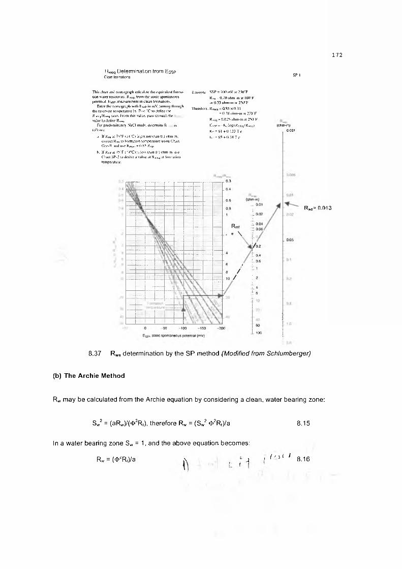
Kweq Determination trom hssp Clean formations SP-1

I b i s chart and nomograph calculate the equivalent forma­tion water resistivity. R trom the static spontaneous potential. Esst». measurem ent in clean formations.

Enter the nom ograph \friih Еч.чи in mV. turning through the reservoir tem perature in F nr "C to define the Rntn^R^cq nitio. From this value. pa&s through the value to define R >v«,.

For predominantly NTaCI muds, determ ine R as follow?:

j . I f Rmf at 7v’ F i '24 'C i is greater than 0.1 ohm-m. correct Rmi to formation tem perature using C han G en-l>. and u.se К.™- = 0 85 R mj-

b. If R,.,r at 75 'F ( ’ I T ) is less than 0.1 ohm-m, u>e Chart SP -2 to derive a value ol R mic4 at formation temperature.

Example SSP = 100 mV a t 250°F

R n,i - 0 .7 0 ohm -m at 100CF or 0.33 ohm -m at 250°F

T herefore. Rr,(M = 0 .3 5 x 0 .3 3 = 0 28 ohm -m at 2501 F

К = 0.025 ohtn-m at 250r F

H >SP = - K c lOgf Rnrfeq/R *ец)Кг = 61 +0.133 T ’F

К, - - 6 5 +0.24 T r

(ohm-m). 0.001

Rwe- 0.013

8.37 Rwe determination by the SP method (Modified from Schlumberger)

(b) The Archie Method

Rw may be calculated from the Archie equation by considering a clean, water bearing zone:

Sw2 = (aRw)/(‘I>2R,), therefore Rw = (Sw2 <I»2R,)/a 8.15

In a water bearing zone Sw = 1, and the above equation becomes:

R w = (<I>‘ R,)/a л . " j I ( r ' ( 1 8.16

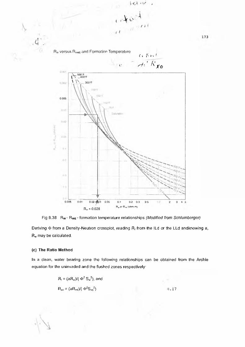
Fig 8.38 Rw- RWe- formation temperature relationships (Modified from Schlumberger)

Deriving Ф from a Density-Neutron crossplot, reading R, from the ILd or the LLd andknowing a,

Rw may be calculated.

(c) The Ratio Method

In a clean, water bearing zone the following relationships can be obtained from the Archie

equation for the uninvaded and the flushed zones respectively:

Rt = (aRw)/( Ф2 Sw2), and

Rxo = (aRmf)/( Ф ^ о 2) 11.17

versus Rweq and Formation Temperature( » Iе- w ■'

7 ! < X o

Rw = 0.028Rw or Rm, (ohm-m)

•4

SP ( M i l l i v o l t s )

Fig 8.39 Rwe determination by the SP method in the presence of a KCI mud Note that when Rmf = Rw, SP * 0 (After Hilchie, 1982)

In such a zone Sw - S*0- 1, and Rw, Ф and a will have the same value. Dividing Rxo by Rt:

Rxo/R, = Rmf/Rw, therefore Rw = Rt Rmf/Rxo 8.18

R, and Rxo are obtained from resistivity logs, and Rmf at formation temperature is known (see

above).

There may be variations in the Rw values determined by the above methods. If this is the case,

then the value obtained by the Archie method should be used, since it will always give a value

of 1.00 for Sw when applied to the water zone. Once determined, Rw is assumed to be constant

throughout the formation being evaluated, unless local knowledge or clear SP log amplitude

changes indicate otherwise.

DETERMINATION OF Sw

In clean formations, Sw may be determined by the direct application of the Archie equation

(equations 8.13 and 8.14). It should be noted that in calculations, the decim al value of Ф must

be used.

DETERMINATION OF S„0

The Archie equation applies also to the flushed zone. However, in this case Rw is replaced by

Rmf (since the flushed zone is assumed to be saturated with mud filtrate), and Rt by Rxo (flushed

zone resistivity):

Sxo = [(aRmf)/(<t>2R*o)]1/2 8.19

Or7 Ss •

Sxo = [ (F R m f) / (R x o ) ]1/2 ' f ~ 8 .2 0

It is important to know S*0 since it gives an indication of hydrocarbon m oveability. Only the

moveable fraction of the hydrocarbons in a reservoir is producible, and can therefore be

regarded as reflecting the recoverable reserves. This fraction, together with all the original

formation water, is displaced from the flushed zone by the invasion of the drilling fluid. Following

invasion, the fraction of the pore volume occupied by moveable hydrocarbons is filled with mud

filtrate. Consequently, water saturation in a flushed zone that originally contained moveable

hydrocarbons increases, i.e. Sxo > S„. The difference between Sx0 and Sw (obtained from the

uninvaded part of the formation) represents the moveable hydrocarbon saturation in a reservoir.

From this it is possible to find the quantity of hydrocarbons displaced by invasion:

Sxo - Sw = moveable oil saturation (MOS), 8.21

and

The ratio S JS m is qualita tive index of hydrocarbon moveability. If S JS m = 1, i.e. Sw = Sxo, no

hydrocarbons have been moved by invasion, implying that any hydrocarbons present are largely

residual. Moveable hydrocarbons are indicated by Sw/Sxo < 0.7 in clastic reservoirs and <; 0.6 in

carbonates.

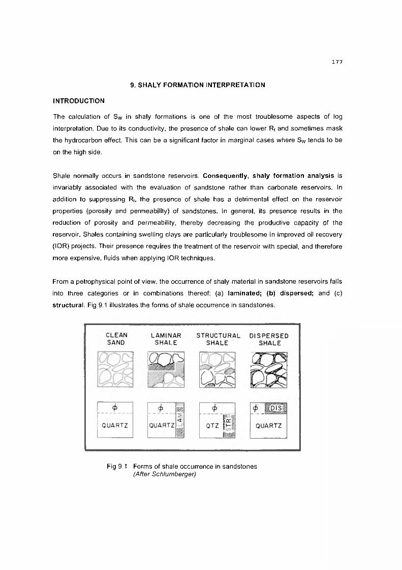
9. SHALY FORMATION INTERPRETATION

INTRODUCTION

The calculation of Sw in shaly formations is one of the most troublesome aspects of log

interpretation. Due to its conductivity, the presence of shale can lower Rt and sometimes mask

the hydrocarbon effect. This can be a significant factor in marginal cases where Sw tends to be

on the high side.

Shale normally occurs in sandstone reservoirs. Consequently, shaly form ation analysis is

invariably associated with the evaluation of sandstone rather than carbonate reservoirs. In

addition to suppressing Rt, the presence of shale has a detrimental effect on the reservoir

properties (porosity and permeability) of sandstones. In general, its presence results in the

reduction of porosity and permeability, thereby decreasing the productive capacity of the

reservoir. Shales containing swelling clays are particularly troublesome in improved oil recovery

(IOR) projects. Their presence requires the treatment of the reservoir with special, and therefore

more expensive, fluids when applying IOR techniques.

From a petrophysical point of view, the occurrence of shaly material in sandstone reservoirs falls

into three categories or in combinations thereof: (a) lam inated; (b) dispersed; and (c)

structural. Fig 9.1 illustrates the forms of shale occurrence in sandstones.

(a) Laminated shale

In this form, thin shale laminations - fractions of an inch to several inches in thickness - are

interspersed with clean sand. The effective porosity and the permeability of the shale are

essentially zero so that the overall porosity and permeability of the formation is reduced in

proportion to the fractional volume of shale. For example, 40% shale will theoretically reduce

effective porosity and permeability to 60% of the clean sand values. Consequently, 30-40%

laminated shale is the maximum amount normally tolerable for production.

(b) Dispersed shale

In this form, shaly material is disseminated in the pore space of the sand. It replaces pore fluid.

This type of distribution is very damaging because a relatively small amount of shale can choke

pores and reduce effective porosity and particularly permeability to non-producible values.

Maximum tolerable clay content is approximately 40% of the sand pore space or about 15% by

volume.

(c) Structural shale

In this form, shale grains, which may be aggregates of shale particles or mudstone clasts, take

the place of sand grains. Porosity and permeability of the sand is affected very little.

Consequently, this type of shale is least objectionable, but it does not occur frequently.

EFFECT OF SHALE ON THE RESPONSE OF LOGGING TOOLS

Measurements of the formation parameters provided by most logging tools are influenced by the

presence of shale in the intervals examined. Table 9.1 summarises the effects of shale on the

responses of the various tools.

The use of uncorrected shale-affected log readings in quantitative interpretation leads to

erroneous results. While the Archie equation gives acceptable Sw values provided Vsh in the

zone of interest is below about 20%, Vsh quantities greater than 20% affect all the parameters in

the equation, particularly Ф and Rt. Uncorrected log data in a shaly reservoir result in Ф values

that are too high and Rt readings that are too low. Consequently, Sw values based on these data

will be too high, and, as mentioned above, may result in the downgrading of the reservoir

concerned. Correcting log readings for the effects of shale requires knowledge of Vsh and some

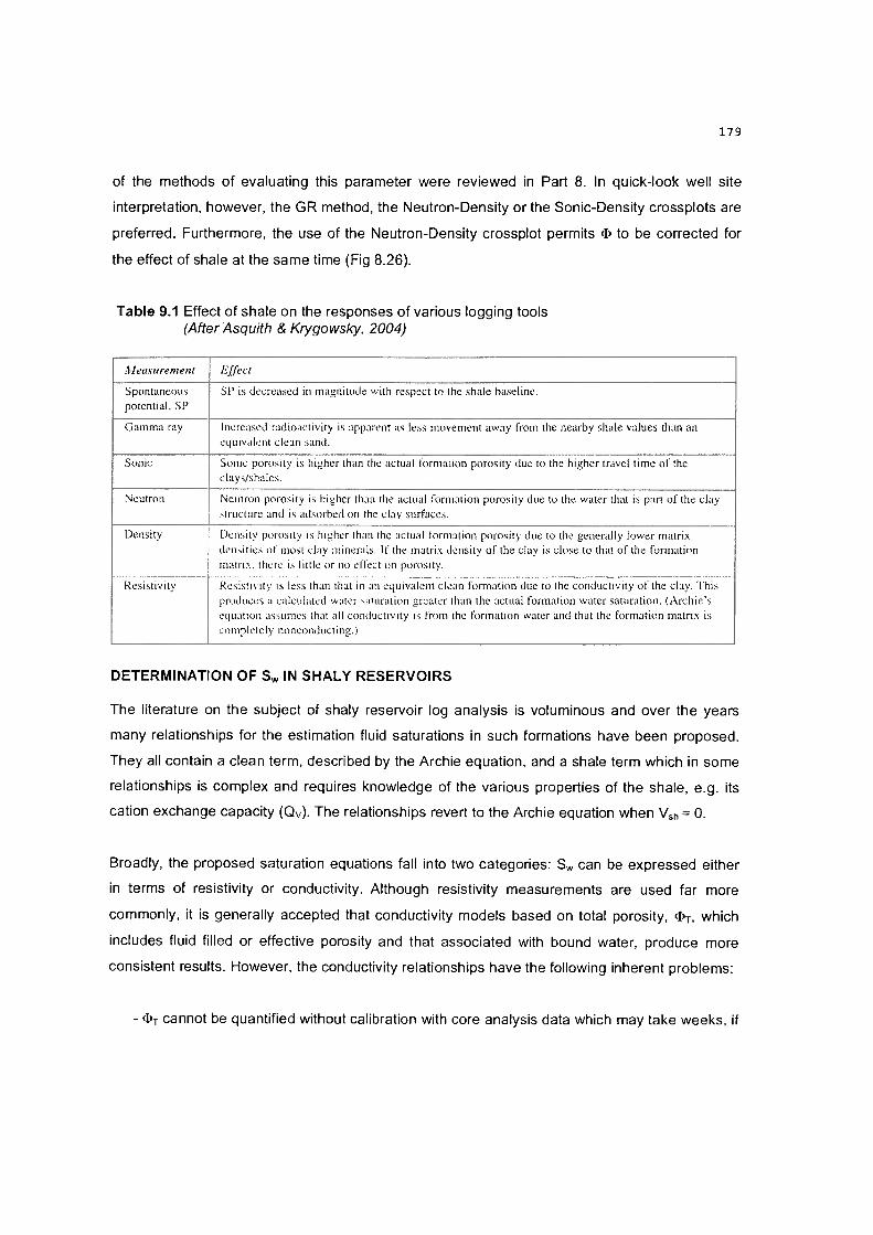
of the methods of evaluating this parameter were reviewed in Part 8. In quick-look well site

interpretation, however, the GR method, the Neutron-Density or the Sonic-Density crossplots are

preferred. Furthermore, the use of the Neutron-Density crossplot permits Ф to be corrected for

the effect of shale at the same time (Fig 8.26).

Table 9.1 Effect of shale on the responses of various logging tools (After Asquith & Krygowsky, 2004)

M easurem en t E ffec t

S p o n ta n eo u s p o te n tia l. SP

S P is d e c rea sed in m ag n itu d e w ith re sp ec t to the sh a le base line .

G a m m a ray In c rea sed rad io ac tiv ity is a p p aren t as less m o v em e n t aw ay from the n ea rb y shale va lu es than an eq u iv a len t c lean sand.

S on ic S om e p o ro s ity is h ig h e r than the ac tu a l fo rm atio n p o ro s ity du e to the h ig h e r trave l tim e o f the c lay s/sh a les .

N eu tron N eu tro n p o ro sity is h ig h e r than the ac tu a l fo rm atio n p o ro s ity due to the w a te r that is part o f the c lay s tru c tu re and is ad so rb ed on the c lay su rfaces .

D ensity D ensity p o ro s ity is h ig h e r than the ac tu a l fo rm atio n p o ro s ity due to the g en era lly lo w er m atrix d e n s it ie s o f m ost clay m inera ls . If the m a trix d en sity o f the c lay is c lo se to that o f the fo rm atio n m atrix , th e re is little o r no effec t on porosity .

R esis tiv ity R es is tiv ity is less than that in an eq u iv a len t c lean fo rm atio n du e to the co n d u ctiv ity o f the clay . T h is p ro d u c e s a ca lcu la ted w a ter sa tu ration g re a te r than the ac tu a l fo rm atio n w a ter sa tu ra tio n . (A rc h ie ’s eq u a tio n assu m es that all co n d u c tiv ity is from the fo rm atio n w a ter and tha t the fo rm atio n m a trix is c o m p le te ly n o n co n d u c tin g .)

DETERMINATION OF Sw IN SHALY RESERVOIRS

The literature on the subject of shaly reservoir log analysis is voluminous and over the years

many relationships for the estimation fluid saturations in such formations have been proposed.

They all contain a clean term, described by the Archie equation, and a shale term which in some

relationships is complex and requires knowledge of the various properties of the shale, e.g. its

cation exchange capacity (Qv). The relationships revert to the Archie equation when Vsh = 0.

Broadly, the proposed saturation equations fall into two categories: Sw can be expressed either

in terms of resistivity or conductivity. Although resistivity measurements are used far more

commonly, it is generally accepted that conductivity models based on total porosity, Фт, which

includes fluid filled or effective porosity and that associated with bound water, produce more

consistent results. However, the conductivity relationships have the following inherent problems:

- Фт cannot be quantified without calibration with core analysis data which may take weeks, if

not months, to generate.

- Cores are not usually taken in shale sections and Фт values derived from low volume clays

in the reservoir may not be representative of those in the adjacent shales.

- Different laboratory methods produce different Фт for the same core.

- The laboratory measurements of Qv and the correlation between these and log data is not

always consistent and can induce errors.

In general, conductivity saturation equations are preferred where sufficient core data are

available, while resitivity models are applied in wildcat wells or where there are insufficient core

analysis results to determine Фт accurately.

A detailed review of the various methods of calculating Sw in shaly formations is beyond the

scope of this course. Instead, two of the most commonly used relationships are presented and

discussed. These are the Indonesia and modified Simandoux equations, the main advantage

of which is that their application does not require Qv data.

Indonesia Equation

This is an empirical formula proposed by Poupon and Leveaux (1971) and considers the

relationship between R, and Sw in terms of the conductivities of the shale in the reservoir,

formation water and any interaction between the two:

(1-Vsh)/2 m/21 /л/Rt = [(Vsh N R sh + Ф N a R w ] Sw 9.1

In terms of conductivity:

n/2 2-Vsh n/2

VCt = V (C w / Fe) S we + V(V<=h C sh) S we 9.2

Ct= Total formation conductivity (1/Rt)

Cw = Conductivity of formation water (1/Rw)

Csh = Conductivity of shale

Fe= ‘Clean’ formation factor

RSh= Resistivity of shale

Swe = Effective (moveable) hydrocarbon saturation

The resistivity equation can be adapted to calculate Sw:

(1-Vsh)/2 m/2 2 -1/nS w ={[(V sh /VRsh + Ф /л/aRw] Rt} 9.3

The chart shown in Fig 9 . 2 solves V Sh 1Vsh/2 graphically. Up to V ci values of 0.3, the slope of the

curve is about 45°, which means that V sh = V sh 1Vsh/z. When V sh = 0, the Indonesia relationship

reverts to the Archie equation

V c la y

Fig 9 . 2 Graphical derivation of V sh 1Vsh/2 (After Schlumberger)

Modified Simandoux Equation

This relationship was proposed by Simandoux ( 1 9 6 3 ) and is based on resistivity, density and

neutron log data. Like the Indonesia model, the Simandoux equation can be expressed in terms

of both resistivity and conductivity:

Sw = 0.4R„/<I> 2['v(5 Ф 2)/(Rw R,) + (Vsh/R sh) - Vsh/R Sh] 9 .4

C t — (C w S w )/F e + V shC 3h 9.5

10. INTRODUCTION TO DIPMETER AND FORMATION IMAGE LOGS

THE DIPMETER LOG

Dipmeter technology was developed in the 1930s and the logs have been available

commercially since the 1950s. Although it is considered by some to be obsolete and replaced by

the current image logs, dipmeter data complement the image logs and are often used in

conjunction with them. The processing and interpretation of dipmeter data are computer based

and various softwares are available for this purpose.

The log provides a continuous measurement of the angle of inclination and the dip direction

(azimuth) of the strata penetrated in the well. Modern dipmeter tools consist of four or six

electrodes mounted on extending arms and record microresistivity. Fig 10.1 shows a four arm

dipmeter device which measures microresistivity at four positions 90° apart around the borehole.

The differences in depth between the curves across the borehole are compared, enabling the

computer to determine dip and azimuth. The principle of measurement and the computation of

dip and azimuth are illustrated in Figs 10.2 and 10.3.

Fig 10.2 Resistivity curves recorded by a four arm dipmeter tool (After Rider, 1996)

tan = —12пп m it i m гл

N К S \V N

Plane orientation: 27/270

Fig 10.3 Dip computation from dipmeter data (After Schlumberger)

Determinations of the angle and direction of dip are usually presented as a plot of ‘tadpoles’

versus depth as shown in Fig 10.4. The head of the tadpole indicates the dip angle and its tail

points to the azimuth. The dip direction can also be displayed as a histogram or fan plot, referred

PAD1

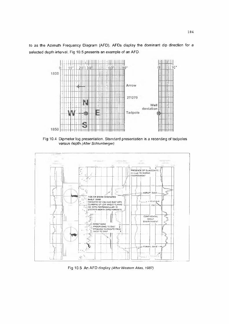
to as the Azimuth Frequency Diagram (AFD). AFDs display the dominant dip direction for a

selected depth interval. Fig 10.5 presents an example of an AFD.

Welldeviation

10°

Fig 10.4 Dipmeter log presentation. Standard presentation is a recording of tadpoles versus depth (After Schlumberger)

1800

The various dipmeter logging tools are listed below:

Company Name of tool Abbreviation Number of pads

High Resolution Dipmeter Tool HDT 4Schlumberger Stratigraphic High Resolution Dipmeter SHDT 4

Oil Based Dipmeter Tool OBDT 4

Diplog Diplog 4Baker Hughes Hexdip Log HDIP 6

High Resolution Dipmeter Tool HEDT 4Malll DUriOn Six Arm Dipmeter SED 6

INTERPRETATION

Dipmeter data have applications in structural and sedimentary geology. In structural geology the

data are used in the interpretation of unconformities, folds and faults, while in sedimentary

geology the dipmeter can assist in facies analysis and palaeocurrent direction studies. It must be

emphasised, however, that dipmeter data should never be interpreted alone and need to be

integrated with other standard logs.

Four patterns are recognised in dipmeter log motifs: green, red, blue and random. These are

illustrated in Fig 10.6.

Green pattern is characterised by constant dip and azimuth with depth and usually represents

post depositional structural dip. It is typical in shale sequences.

Red pattern represents uniform azimuth but the dip angle decreases upward. This pattern is

usually associated with folds, faults, unconformities, reefs, channel sands and valley fills (Figs

10.7-10.12).

Fig 10.7 Dipmeter motif associated with a tilted, asymmetrical anticline(After Western Atlas, 1987)

Fig 10.9 Dipmeter motif associated with a thrust (After Western Atlas, 1987)

Blue pa tte rn exhibits roughly uniform azimuth but an upward increase in dip angle. This pattern

is usually associated with folds or faults, unconformities, palaeocurret directions and submarine

fan deposits (Figs 10.13 and 10.14).SP TRUE DIP П

0 Ю 20 30 Л0

Fig 10.13 Dipmeter blue patterns showing sediment transport direction (After Western Atlas, 1987)

Random pattern shows scattered dip and azimuth. Massive beds lacking coherent bedding

planes or slumped deposits may be responsible for such a response. It may also result from tool

malfunction or poor borehole conditions causing the pads to lose contact with the borehole wall.

FORMATION IMAGE LOGS

Image logs were introduced in the mid-1980s and have undergone rapid development in terms

of both data acquisition technology and image production. The tools do not, however, produce

pictures or photographs of the borehole wall; they provide a computer generated image based

on the measurement of the resistivity or the acoustic reflectivity of the formations surrounding

the borehole. The measurements are limited to the borehole wall and do not penetrate the

formations.

Both wireline and LWD imaging tools are available. Wireline dvices produce high resolution

microresistivity, micro-induction and acoustic images, suitable for detailed structural and

sedimentological analyses. LWD tools generate microresistivity and density images that can be

transmitted to the surface via mud pulses in real time or from data stored in memory and

downloaded when the device is recovered from the borehole.

Imaging tools fall into electrical and acoustic categories, which are briefly described below.

ELECTRICAL IMAGE TOOLS

These are based on dipmeter technology and have pad mounted microresistivity electrodes

which are pressed against the borehole wall. They provide partial coverage of the borehole wall,

operate in conductive water based mud only and have a vertical sampling interval of 0.25cm.

The various electrical imaging tools are listed below:

Company Name of Tool Abbreviation Number of pads

Schlumberger Formation Micro Scanner FMS 4

Schlumberger Formation Micro Imager FMI 8

Baker Hughes SimulTaneous Acoustic and Resistivity Imager

STAR 6

Halliburton Electrical Micro Imaging EMI 6

Fig 10.15 presents the FMI and STAR imaging tools.

(After Schlumberger) (After Baker Hughes)

Fig 10.15. Electrical imaging tools

ACOUSTIC (ULTRASO NIC) IMAGE TOOLS

Also known as borehole televiewers (BHTV), these tools provide full coverage of the borehole

wall, operate in any fluid including oil based mud and are run centred in the well. A rotating

transducer emits and records signals and the vertical sampling interval depends on the logging

speed. Generally, it is between 180 and 250 samples per revolution which is between 6 and 12.

The sound waves emitted by the transducer are reflected by the borehole wall and the transit

time of the first echo and the first echo amplitude are recorded and processed into images. The

operating and measurement principles of the device are illustrated in Figs 10.16 and 10 17.

Fig 10.16 Schematic representation of the operating principle of the acoustic imaging tool (From A squ ith and Krygowski, 2004)

FocusedTransducer

\

Wall

Pulse Transit T im e Echo 1UBI sign, i Л / First echo amplitude

UBI measurements:• Transit time of first echo: distance - speed in mud x Transit time / 2

=> Transit Time image (borehole radii)

• First echo amplitude => amplitude image

Fig 10.17 Principle of measurement of the acoustic imaging tool (After Schlumberger)

The various acoustic imaging tools are listed below

Company Name of tool Abbreviation

Schlumberger Ultrasonic Borehole Imager UBI

Baker Hughes Circumferential Borehole Image Log CBIL

Baker Hughes SimulTaneous Acoustic and Resistivity Imager STAR

Halliburton Circumferential Acoustic Scanning tool CAST

IMAGE INTERPRETATION

The standard presentation of image logs is to split or unwrap the borehole along true north and

unroll the cylinder into a flat strip. Real horizontal and vertical planes will appear as horizontal

and vertical features on the log. Dipping surfaces intersecting the well, however, will appear as a

sine wave, as demonstrated in Fig 10.18 The high point of the surface as it intersects the well is

represented by the crest of the sine curve and the steeper the dip, the greater the wave

amplitude.

Iri electrical image logs conductive, low resistivity features such shales and fluid filled fractures

After Rider, 1996

After Asquith and Krygowsky, 2004

Fig 10.18 Representation of dipping surfaces on image logs

are displayed as dark colours, while high resistivity features such as sandstones and carbonates

are shown as lighter shades of brown, yellow and white. In the case of the acoustic image logs,

low amplitude or high transit time features such as shales, borehole irregularities (washouts) and

fluid filled fractures are represented as dark colours. Sandstones and carbonates, charaterised

by high amplitude or low transit times, are displayed in lighter shades of brown, yellow and white

(Fig 10.19).

Low amplitude/resistivity High amplitude/resistivity

Fig 10.19 Image log colour codes

Image processing falls into two categories - static and dynamic. Static images are produced by

applying a single colour contrast setting to the entire well. In the case of dynamic images, a

variable colour contrast is applied in a ‘window’ that moves along the borehole. This improves

image quality and enhances views of features such as bed boundaries, fractures and vugs.

N : f s W

\ r\1 j. \ \ f \ Л\ ! 1 \ 1 \ 1 \ I \\ \ ' \ i\

i \\\ 1 \

V'- -

Image logs have a wide variety of applications. As with all log data, they should not be

interpreted in isolation and the best results are obtained by combining them with information

from other sources. The most common applications of image logs include the detection of faults

and fractures (Figs 10 20 and 10.21), borehole breakouts (Fig 10.22 and 10.23), stratigraphic

characteristics such as bedding (Fig 10.24) and identification of sedimentary features such as

cross bedding, slumping and texture (Figs 10.25-10.27).

Fig 10.20 Normal fault detection from FMI (After Schlumberger)

In-sttu Stress Directions

FA»xjfTx*n horizontal Stre*» dkbCDcn

Borer>ote b re a ko u tsглгатишРюгиотшwua

drecfon

tnducodIracfurr*

naturai

* 4 r

Г'Ю ЯТН

Fig 10.22 Illustration of breakout (After Schlumberger)

Fig 10.23 A fractured sand and shale interval from CBIL. Borehole breakouts (B) appear as dark patches 180° apart from each other(After Asquith and Krygowsky, 2004)

■ ■ ■ ,•

3*r

Fig 10.24 Regular bedding from LWD Startrack (After Baker Hughes)

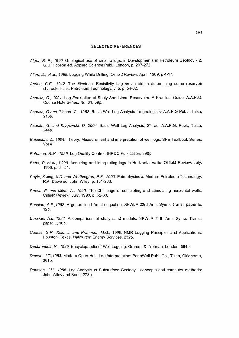
SELECTED REFERENCES

Alger, R. P., 1980. Geological use of wireline logs: in Developments in Petroleum Geology - 2, G.D. Hobson ed. Applied Science Publ., London, p. 207-272.

Allen, D., et a!., 1989. Logging While Drilling: Oilfield Review, April, 1989, p 4-17.

Archie, G.E., 1942. The Electrical Resistivity Log as an aid in determining some reservoir characteristics: Petroleum Technology, v. 5, p. 54-62.

Asquith, G., 1991. Log Evaluation of Shaly Sandstone Reservoirs: A Practical Guide, A.A.P.G. Course Note Series, No. 31, 59p.

Asquith, G and Gibson, C., 1982. Basic Well Log Analysis for geologists: A.A.P.G Publ., Tulsa, 216p.

Asquith, G. and Krygowski, D, 2004. Basic Well Log Analysis, 2nd ed: A.A.P.G. Publ., Tulsa, 244 p.

Bassiouni, Z , 1994. Theory, Measurement and interpretation of well logs: SPE Textbook Series, Vol 4

Bateman, R.M., 1985. Log Quality Control: IHRDC Publication, 398p.

Betts, P. et a!., I 990. Acquiring and interpreting logs in Horizontal wells: Oilfield Review, July, 1990, p. 34-51.

Boyle, K,Jing, X.D. and Worthington, P.F., 2000. Petrophysics in Modern Petroleum Technology, R.A. Dawe ed, John Wiley, p. 131-206.

Brown, E. and Milne, A., 1990. The Challenge of completing and stimulating horizontal wells: Oilfield Review, July, 1990, p. 52-63.

Bussian, A .E .,1982. A generalised Archie equation: SPWLA 23rd Ann. Symp. Trans., paper E, 12p.

Bussian, A .E .,1983. A comparison of shaly sand models: SPWLA 24th Ann. Symp. Trans., paper E, 16p.

Coates, G.R., Xiao, L. and Prammer, M.G., 1999. NMR Logging Principles and Applications: Houston, Texas, Haliburton Energy Services, 232p.

Desbrandes, R., 1985. Encyclopaedia of Well Logging: Graham & Trotman, London, 584p.

Dewan, J. Т.,1983. Modern Open Hole Log Interpretation: PennWell Publ. Co., Tulsa, Oklahoma, 361p.

Doveton, J.H.. 1986. Log Analysis of Subsurface Geology - concepts and computer methods: John Wiley and Sons, 273p.

Dresser Atlas, 1982. Well Logging and Interpretation Techniques. The Course for Home Study, 2nd ed.

DresserAtlas, 1985. Log Inteipretation Charts: 157p.

Elliott, H.W., 1983. Some 'Pitfalls' In Log Interpretation: Log Analyst, v. 24, p. 10-24.

Ellis, D.V., 2007. Well Logging for Earth Scientists, 2nd ed: Springer, 692p.

England, R.E., 1975. Well Log Interpretation: Birdwell Div., Seismograph Service Corp., Tulsa, Oklahoma.

Fertl, W.H. (ed.), 1976. Abnormal Formation Pressures - Implications to Exploration, Drilling and Production of Oil and Gas Resources: Elsevier, Amsterdam.

Fertl, W.H., 1984. Advances in well logging interpretation: Oil and Gas Journal, April 16th, p. 85-91.

Hansen, R.R. and White, J., 1991. Features of Logging While Drilling: SPE/IADC Conf., Amsterdam, Paper 21989.

Hatton, I.R., Reeder, М., Newman, M. St J. and Roberts, D., 1992: Techniques and applications of petrophysical correlation in submarine fan environments, early Tertiary sequence, North Sea: in Geological Applications of Wireline Logs II, A. Hurst, C.M. Griffiths & P.F. Worthington eds, Geol Soc Spec Pub No 65, p. 21-30.

Helander, D.P., 1983. Fundamentals of Formation Evaluation: Oil and Gas Consultants Int. Publ., 332p.

Heslop, A., 1975. Porosity in shaly-sands: SPWLA, 16th Ann. Symp. Trans., Paper F. 12p.

Hilchie, D.W., 1982a. Applied openhole log Interpretation: D.W. Hilchie Inc., Golden, Colorado, 330p.

Hilchie, D.W., 1982b. Advanced Well Log Interpretation: D.W. Hilchie Inc., Golden, Colorado.

Jenkins, R.E., 1960. Accuracy of porosity determinations: First SPWLA Logging Symp., Tulsa, Oklahoma.

Merkel, R.H., 1979. Well Log Formation Evaluation: A.A.P.G. Continuing Education Series, No. 14, 82p.

Meyer, B.L. and Nederlof, M.H., 1984. Identification of source rocks on wireline logs by density/resistivity and sonic transit time/resisivtity crossplots: A.A.P.G. Bull., v. 68, p. 121-29.

Misk, A., Mowat, G., Goetz, J. and Vivet, B., 1977. Effects of hole conditions on log measurements and formation evaluation: SAID 5th Ann. European Symp. Trans., Paris, Comm. 22, 16p.

Patchett, J.G. and Coalson, E.B., 1979. The determination of porosity in sandstones and shaly

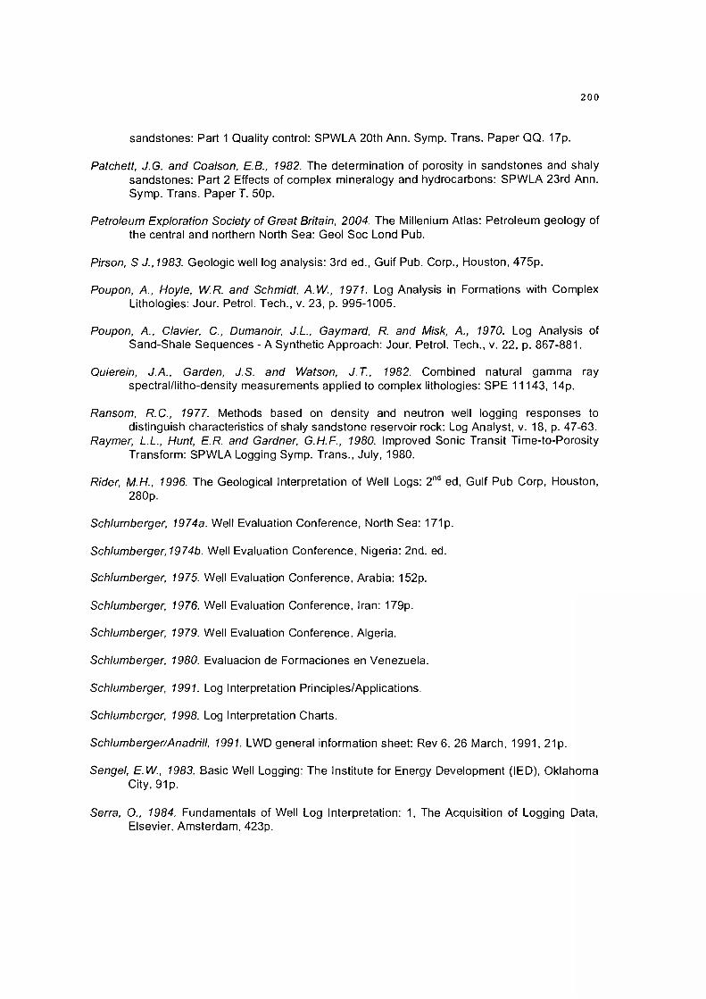
sandstones: Part 1 Quality control: SPWLA 20th Ann. Symp. Trans. Paper QQ. 17p.

Patchett, J.G. and Coalson, E.B., 1982. The determination of porosity in sandstones and shaly sandstones: Part 2 Effects of complex mineralogy and hydrocarbons: SPWLA 23rd Ann. Symp. Trans. Paper T. 50p.

Petroleum Exploration Society o f Great Britain, 2004. The Millenium Atlas: Petroleum geology of the central and northern North Sea: Geol Soc Lond Pub.

Pirson, S J., 1983. Geologic well log analysis: 3rd ed., Guif Pub. Corp., Houston, 475p.

Poupon, A., Hoyle, W.R. and Schmidt, A.W., 1971. Log Analysis in Formations with Complex Lithologies: Jour. Petrol. Tech., v. 23, p. 995-1005.

Poupon, A., Clavier, C., Dumanoir, J.L., Gaymard, R. and Misk, A., 1970. Log Analysis of Sand-Shale Sequences - A Synthetic Approach: Jour. Petrol. Tech., v. 22, p. 867-881.

Quierein, J.A., Garden, J.S. and Watson, J.T., 1982. Combined natural gamma ray spectral/litho-density measurements applied to complex lithologies: SPE 11143, 14p.

Ransom, R.C., 1977. Methods based on density and neutron well logging responses to distinguish characteristics of shaly sandstone reservoir rock: Log Analyst, v. 18, p. 47-63.

Raymer, L.L., Hunt, E.R. and Gardner, G.H.F., 1980. Improved Sonic Transit Time-to-Porosity Transform: SPWLA Logging Symp. Trans., July, 1980.

Rider, M.H., 1996. The Geological Interpretation of Well Logs: 2nd ed, Gulf Pub Corp, Houston, 280p.

Schlumberger, 1974a. Well Evaluation Conference, North Sea: 171 p.

Schlumberger,1974b. Well Evaluation Conference, Nigeria: 2nd. ed.

Schlumberger, 1975. Well Evaluation Conference, Arabia: 152p.

Schlumberger, 1976. Well Evaluation Conference, Iran: 179p.

Schlumberger, 1979. Well Evaluation Conference, Algeria.

Schlumberger, 1980. Evaluacion de Formaciones en Venezuela.

Schlumberger, 1991. Log Interpretation Principles/Applications.

Schlumberger, 1998. Log Interpretation Charts.

Schlumberger/Anadrill, 1991. LWD general information sheet: Rev 6, 26 March, 1991, 21 p.

Sengel, E.W., 1983. Basic Well Logging: The Institute for Energy Development (IED), Oklahoma City, 91 p.

Serra, O., 1984. Fundamentals of Well Log Interpretation: 1, The Acquisition of Logging Data, Elsevier, Amsterdam, 423p.

Serra, О., 1986. Fundamentals of Well Log Interpretation; 2. The Interpretation of Logging Data: Elsevier, 684p.

Simandoux, P., 1963. Mesures dielectriques en milieu poreux, application a mesure saturation en eau: Etude du Comportement des Massifs Argileux: Revue de I’instutu Francais du Petrole, Supplementary Issue (Translated text in SPWLA Reprint Volume Shaly Sand, July 1982).

Society o f Professional Well Log Analysts, 1975. Glossary of terms and expressions used in well logging: SPWLA publ., Houston, Texas, 74p.

Thomas, D.H., 1977. Seismic applications of sonic logs: SPWLA 5th European Symp., Trans., Paris, Paper 7, 24p.

Threadgold, P., 1971. Some problems and uncertainties in log interpretation: SPWLA 12th Ann. Symp. Trans., Paper W. 19p.

Welex, 1978. An Introduction to Well Log Analysis: Houston, Texas, 46p.

Wyllie, M.R.J., Gregory, A.R. and Gardner, G.H.F., 1956. Elastic Wave Velocities in Heterogeneous and Porous Media: Geophysics, v. 21, No. 1, p. 41-70.

Wyllie, M.R.J., Gregory, A.R. and Gardner, G.H.F., 1958. An Experimental Investigation of Factors Affecting Elastic Wave Velocities in Porous Media: Geophysics, v. 23, No.3, p. 459-93.

Worthington, P.E., 1985. The Evolution of Shaly-Sand Concepts in Reservoir Evaluation: The Log Analyst, v. 26, No. 1, p. 23-40.