1

Impacts of Remotely-Sensed Vegetation Dynamics on Hydrologic Response in a

Semiarid Mountain Watershed

Taufique H. Mahmood and Dr. Enrique R. Vivoni (advisor)

Final Report April 30, 2008

Department of Earth and Environmental Science New Mexico Institute of Mining and Technology.

2

1. Introduction Vegetation is an important characteristic in forested mountain watersheds due to its extensive spatial coverage, its interaction with hydrology (e.g. Band et al., 1993; Sandvig and Phillips, 2006) and its spatiotemporal variability (e.g. Alves, 2002). The thick vegetation covers in a forested watershed intercept precipitation (e.g. Gash et al., 1995; Crockford and Richardson, 2000), uptake water from soil for transpiration (e.g. Roberts, 1983; Granier et al., 1996), cause shading on the hillslopes (e.g. Buttle et al., 2005), impacts erosion and runoff (Bosch and Hewlett, 1982), increases relative humidity, capture fractions of snowfall (e.g. Hedstrom and Pomeroy, 1998) and impact mass balance and energy balance of hydrologic system (Lee, 1980; Eaglesoon, 2002). Therefore, vegetation dynamics significantly influence the basin hydrologic response by impacting evapotranspiration, throughfall and interception.

Climatic seasonality is an important phenomenon in controlling spatiotemporal vegetation dynamics. Seasonality in radiation and precipitation leads to vegetation changes such as biomass, vegetative fraction, greenness, growth, stomata resistance and albedo (e.g. Aber et al., 1995; Small and Kurc, 2003). These dynamics eventually impact hydrologic responses such as interception, throughfall, sap-flow and evapotranspiration. Hdrometeorological variables such as precipitation, air temperature, relative humidity and wind speed control the climatic seasonality in forested mountain watersheds. Remotely sensed images are a source of spatiotemporal data for characterizing watershed conditions such as soil and vegetation (Jensen, 1996). Satellite sensors capture a large overview of the land surface by viewing earth surface from high altitudes (~700 km). They generally receive the reflected electromagnetic energy by different land covers at different wavelengths of electromagnetic spectrum. Most government and privately-owned satellite sensors capture imagery in visible, near infrared, shortwave infrared band and thermal infrared bands, which provide the spectral details of land covers with high spatial resolution (1m to 30 m). The visible, near infrared and shortwave infrared bands provide detailed information about the shortwave albedo of vegetation (Liang et al., 1999; Liang et al, 2000), whereas the near infrared and red bands provide the indirect information about the vegetation fraction (Choudhury, 1984), health of vegetation (Jensen, 1996) and stomata resistance (Carter, 1998). Since the launch of first Landsat sensor in 1972, researchers have been successfully using satellite imagery for land cover change detection (e.g. Coppin and Bauer, 1996; Singh, 1989). The remotely sensed datasets appeal to the hydrologic research community due to their detailed spectral and spatial resolution of watershed characteristics (Schultz, 1996). Distributed hydrologic models are useful tools for examining the influences of spatiotemporal vegetation dynamics on hydrologic responses because distributed models have the capacity to produce spatially explicit fields of hydrologic variable at a range of time intervals (e.g., Western et al., 1999; Ivanov et al., 2004a). Distributed models are based on physical representation of hydrologic process occurring in a watershed and consider the spatial variability of soil, vegetation, rainfall and topographic characteristics (Anderson et al., 2001; Ivanov et al., 2004a; Ivanov et al., 2008). Evaluation of

3

distributed hydrologic models is a real challenge in the scientific community, as these require spatiotemporal observations of a number of interrelated variables at distributed locations in the basin. Limited sets of studies (e.g. Motovilov et al., 1999; Western et al., 1999; Anderson et al., 2001) have compared distributed hydrologic responses with observations at distributed locations. The current project has investigated the impacts of remotely sensed seasonal vegetation dynamics in hydrologic responses using distributed hydrologic model. The objectives of current study were to capture seasonal vegetation dynamics from remotely sensed datasets and incorporate them into distributed hydrologic models to investigate the impacts of vegetation changes in hydrologic responses. Therefore, the objectives of this study were two fold; one was to capture remotely sensed vegetation dynamics from remotely sensed imagery, and another was to incorporate the captured vegetation dynamics into a distributed hydrologic model to investigate the impacts on hydrologic responses. The current project has focused on simulating the Redondo watershed for 2005 monsoon, as field observations are available for evaluation of simulated results. 2. Study area

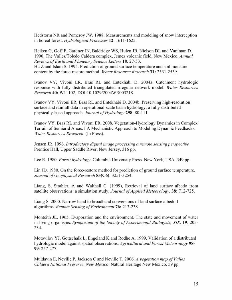
The study area is a small mountain watershed (Redondo Creek basin), located in the eastern part of Jemez River basin in north-central New Mexico (Figure 1). The Jemez River basin is one of the forested mountainous headwaters for the Rio Grande in New Mexico (Ellis et al., 1993; Fromento-Trigilio and Pazzaglia, 1998). The area of the watershed is ~30 km2. The majority of tributaries of Redondo Creek drain to the East Fork of the Jemez River. A topographic representation of the study area was derived from a USGS 10 m digital elevation model (DEM) (Figure 1c). The basin topography is characterized by the Redondo Peak resurgent volcanic dome and the Redondo graben. High elevations (> 2850m) are observed at Redondo Peak and its surrounding areas in the eastern part of study site, whereas low elevations (2300-2600m) are observed along Redondo Creek. Redondo Creek and the majority of its tributaries originate from Redondo Peak and form a radial drainage pattern (Fromento-Trigilio and Pazzaglia, 1998). Most of tributaries of the Jemez River are perennial due to continuous base flow from groundwater through springs and seepage (Goff and Gardner, 1994; Rao et al., 1996). Figure 1c also shows the locations of the soil moisture observations (sampling points), an inactive USGS stream gauge and the existing weather station in the study area.

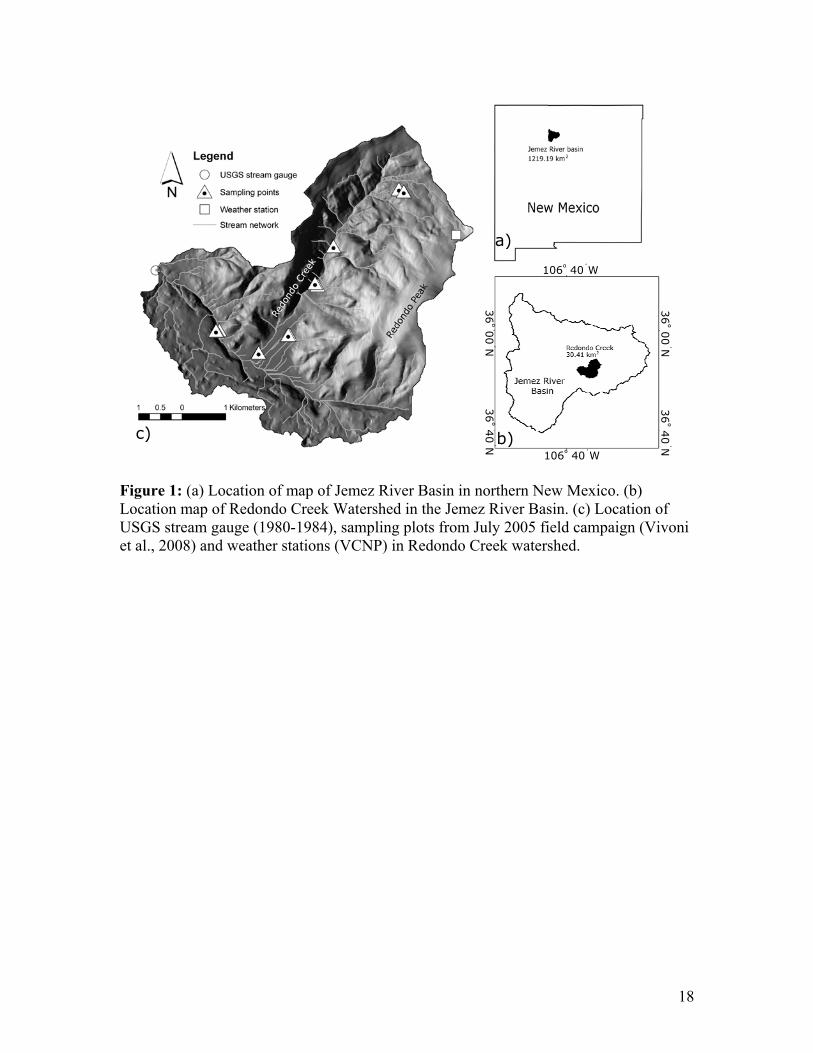
Redondo creek basin exhibits a high spatial variability (Figure 2a) in ecosystem

distribution with strong links to elevation, slope and aspect (Mauldavin et al., 2006; Coop and Givnish, 2007). Mauldvin et al. (2006) mapped 20 different forest units based from high spatial resolution (2 m) color (RGB) digital areal photographs with the aid of 369 ground truth points and two Landsat scenes (Figure 2a). Spruce-fir (Picea pungens) forest occupies high elevations areas around Redondo peak, while ponderosa pine (Pinus ponderosa var. scopulorum), mixed conifer, aspen (Populas tremuloides) and Gambel Oak (Quercus gambelii) forests occur generally at steeper hillslopes. Forest meadows and grasslands occupy the floodplain and gently sloping areas at lower elevation. Grasslands of the study area are strongly tied to slope inclination, aspect, soil moisture and elevation

4

(Coop and Givnish, 2007a). Coop and Givnish, (2007b) show a strong evidence of rapid and continuous forest encroachment into the grasslands at steep and high elevation slopes and slower and more episodic invasion at valley bottoms over last century.

Soils of the study site are also characterized by spatial variability (Figure 2b) and

are strongly tied to the geomorphology of the study area. The soil matrix contains coarse grain materials, such as boulders, cobbles and pebbles in higher amounts, within areas of active tectonics and in the relatively steeper hillslopes. Coarse sandy loam soils occur at Redondo Peak and its surrounding areas, whereas silty and clay loam soils occur in floodplain areas. The surficial rock types are covered by relatively thick soil layer in most areas, with few exceptions. Sparsely vegetated patches of brecciated rhyolite (Talus slope) bordered by high angle normal faults are exposed in Redondo Peak. Soil types are also linked to the geology of the watershed which is characterized by a Pleistocene caldera system and interior resurgent dome (Goff et al., 1996; Heiken et al., 1990). The exposed rock types are primarily ignimbrite, rhyolite, basalt and pumice in Redondo Peak, while alluvium and lacrustine deposits dominate the valley bottoms. 3. Methods The goals of this project are to investigate remotely sensed vegetation dynamics in hydrologic responses. The task required to accomplish this goal are:

• To capture remotely vegetation dynamics from Landsat and MODIS imagery. • To incorporate the vegetation dynamics into distributed hydrologic model. • To evaluate model results with available observations.

The following section describes the remote sensing technique and datasets, distributed hydrologic model and available observations to evaluate the model results. 3.1. Vegetation dynamics using remote sensing: The available remotely sensed datasets for this study are listed in Table 1 with spatial and spectral characteristics. The remote sensing products are Landsat5 TM and MODIS imagery used to capture short-term vegetation dynamics. The analyses of remotely sensed data are always divided into two parts. One is image preprocessing and another is land surface information extraction of processed datasets. The tasks regarding image preprocessing include the radiometric and geometric corrections and topographic normalization. The tasks of land surface information extraction include on screen digitization of different land cover, automated feature extraction, image classification using different classifier and quantification of vegetation biophysical properties using developed technology. 3.1.1. Preprocessing tasks of remotely sensed datasets: The preprocessing tasks include radiometric correction, geometric correction and topographic normalization. Generally, vendors provide the imagery with standard

5

radiometric correction. The remote sensing products are provided from the USGS with standard radiometric correction using NLAPS method. The imagery are geometrically corrected with reference to Universal Transverse Mercature projection (zone 13) with GRS 1980 spheroid and North American Datum 1983. Topographic normalizations are required in this study due to severely undulated and rugged surface of the watershed. Lambertian reflection model (Colby 1991; Smith et al., 1980) is used for topographic normalization in this study. The equations for topographic normalization are given below:

where BVnormalλ= topographically normalized albedo, BVnormalλ= observed albedo, i = angle between solar rays and normal to the surface, θs = sun elevation angle, θn= sun azimuth angle and φs = slope of the earth surface. 3.1.2. Extraction of vegetation dynamics The current research has captured spatiotemporal variation of vegetation biophysical properties such as albedo and vegetation fraction from Landsat5 TM and MODIS imagery. The advantages of using Landsat5 TM imagery are high spectral resolutions (seven bands), moderate spatial resolution (30 m) and 16 days temporal resolution, whereas the advantages of using MODIS imagery are high temporal resolution (daily) and high spectral resolution. However, the Landsat5 TM is costly whereas MODIS imagery has no cost. On the other hand, the spatial resolution of Landsat5 TM (30 m) is higher than the MODIS imagery (250-500 m). The current research uses both Landsat5 TM and MODIS imagery for capturing vegetation dynamics. Optical imagery are useful during monsoon period due to more cloud free days. The current project has quantified short wave albedo and vegetation fraction. The short wave land cover albedo is estimated using the following equation for a Landsat5 TM image (Liang et al., 1999):

where λshortwave is the shortwave for particular pixel, λ1 is albedo at band 1 (blue), λ3 is albedo at band 3 (red), λ4 is albedo at band 4 (near infrared), λ5 is albedo at band 5 (short wave infrared), λ7 is albedo at band 7 (short wave infrared). The albedo for MODIS image is calculated using following equation: where λshortwave is the shortwave albedo for particular pixel, λ1 is albedo at band 1 (red), λ2 is albedo at band 2 (near infrared), λ3 is albedo at band 3 (blue), λ4 is albedo at band 4

(1) cos(i)

BVBV λ observed

λ normal =

(3) 0.072λ0.085λ0.373λ0.13λ0.356λλ 75431shortwave ++++=

7654321shortwave λ06.0λ01.00.16λ0.26λ0.34λ0.23λ0.39λλ +−+−++= (4)

(2) )φ)cos(φ)sin(θθsin(90))cos(θθcos(90cos(i) nsnsns −−+−=

6

(green), λ5 is albedo at band 5 (short wave infrared), λ6 is albedo at band 6 (short wave infrared) and λ7 is albedo at band 7 (short wave infrared). Vegetative areal fraction is an important vegetation parameter for assessing basin hydrologic responses because it impacts directly interception and evapotranspiration. This research works uses vegetation fraction defined by Choudhury et al., 1994: where f is vegetation fraction, VI represents vegetation index, VImax is the seasonal maximum of vegetation index, VI is the vegetation of particular pixel, VImin is the seasonal minimum of vegetation index, ζ=0.7 for planophile canopy and ζ=1.4 for erectophile canopy. The current research uses NDVI (Normalized Difference Vegetation Index) as vegetation index (VI) in equation 5. The NDVI is defined as:

where λNIR is the albedo at near infrared band and λR is the albedo at red band. 3.2. Distributed hydrologic modeling

We apply the tRIBS model in this study for soil moisture simulations in Redondo

Creek. The tRIBS model is a fully distributed model, which considers physical representations of hydrological processes and captures distributed watershed and hydrometeorological characteristics (Ivanov et al., 2004a; Ivanov et al., 2004b; Vivoni et al., 2005). Modeling tasks using tRIBS include physical representation of watershed, parameterizations and model testing based on the comparison between simulated output and observations (e.g. Ivanov et al., 2004b). tRIBS can be forced with spatiotemporal precipitation fields and parameterized soil and vegetation fields. Model outputs include spatiotemporal fields of soil moisture over different soil depths, evapotranspiration, interception and runoff generations among other variables. Soil moisture is distributed in the model by vertical and lateral fluxes that account for soil properties, the influence of topography and the effects of vegetation canopy (Ivanov et al., 2004b).

3.2.1. Watershed representation

The physical representations of a watershed in the model are based on a triangulated irregular network (TIN) constructed from a grid-based DEM to retain hydrologic features such as stream networks and watershed divide as well as internal ridges (Vivoni et al., 2004). The advantages of using a TIN based surface include the reduction of the number of computational nodes without loss in terrain variability, the flexibility of representing watershed at multiple resolutions and the preservation of linear features. The current study has discretized the Redondo Creek watershed. The following describes the discretization of Redondo Creek watershed to demonstrate watershed representations in tRIBS model.

(5) )VIVI

VIVI(1f ζ

1

minmax

max

+−

−=

(6) λλλλ

NDVIRNIR

RNIR

+−

=

7

For the Redondo Creek, the current study has used 0.25 km2 threshold to delineate the stream networks from the 10 m DEM following the method of O’Callaghan and Mark (1984). To delineate the threshold, we compared the modeled stream network for different area thresholds with an existing drainage map and the concave upward regions of high resolution (1 m) areal photograph. We choose the two parameters of a floodplain extraction model (height and minimum stream order) by overlaying the constructed floodplain areas on the high-resolution color photographs, which provided the details on vegetation distribution and saturation of near-stream regions. The stream network representations and the floodplain areas were incorporated into the TIN model at high resolution (e.g. 30 m spacing retained between channel node and floodplain elements).

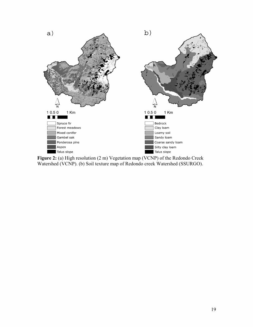
The overall resolution of the TIN depends on the allowable elevation difference (Zr) between TIN surface and the DEM. Vivoni et al. (2005) detailed the selection of the Zr proposed a method for a prior determination based on the sensitivity of topographic attributes. To carry this out, the horizontal point density (d) defined as the ratio of number nodes in TIN to original DEM nodes, and the Root mean square error (RMSE) between TIN elevations and DEM elevations are used. For Redondo Creek, horizontal point density decreases (decreasing computational nodes) with increasing Zr whereas the RMSE increases (decrease in elevation accuracy) with increasing of Zr (Figure 3a). These analyses aim to capture the topographic variability in the DEM with minimum number of computational nodes while preserving the hydrologic response of the high-resolution domain (Vivoni et al., 2005). Figure 3b shows that percent change in mean slope, mean elevation and mean convex upward curvature with respect to finest TIN resolution (d = 1). Large changes in slope and curvature occur for d < 0.2 while minimum differences are observed for higher resolutions. We selected d = 0.2 (only twenty percent nodes of original DEM nodes are retained) with Zr=6 m and RMSE = 0.45 m for the Redondo Creek. Figure 4 illustrates the TIN surface using d = 0.2 with the embedded floodplain and stream network. This representation captures the Voronoi polygons, derived from the TIN, which serves as the basic model elements (Vivoni et al., 2005).

3.2.2. Model forcing

Model can be forced by hydrometeorological parameters such as precipitation, air temperature and relative humidity. The tRIBS model also provides the flexibility to input climate forcing as spatiotemporal grids. The current research has forced the model with hourly NEXRAD radar precipitation and Redondo weather station observation of relative humidity and air temperature.

8

3.2.3. Hydrological processes

3.2.3.1. Interception:

The model uses Rutter canopy water balance model (Rutter et al., 1971; Rutter et al., 1975) for rainfall interception. It accounts for changes in the canopy storage with the rainfall rate, canopy drainage and potential evapotranspiration rate. Canopy water dynamics depends on species type and climatic seasonality. The input vegetation parameters for interception processes are free throughfall coefficient and vegetation fraction, which influences interception process in the model. 3.2.3.2. Surface energy model The tRIBS model accounts for short wave and long wave components of radiation for geographic locations, time of the year, aspect and slope during simulations (Bras, 1990). The tRIBS model also utilizes combination equation (Penman, 1948; Monteith 1965), gradient method (Entekhabi, 2000) and force-restore (Lin, 1980; Hu and Islam, 1995) method to estimate the latent, sensible and ground heat fluxes at land surface. Root zone soil moisture content and top soil layer moisture content restricts evapotranspiration from vegetated surface and bare soil surface. Vegetation fractional extent of each Voronoi polygon controls the partitioning of latent heat energy into vegetation transpiration, bare soil evaporation and evaporation of wet canopy. 3.2.3.3. Infiltration The tRIBS model accounts for infiltration under both ponded and unsaturated conditions (Ivanov et al., 2004a). Soil heterogeneity is represented by assuming exponential decays of saturated hydraulic conductivity with normal depth (Beven, 1982; Beven, 1984; Harr, 1977). Soil layering in all direction is depicted by anisotropy coefficient ratio defined as the saturated conductivity parallel to soil surface direction to saturated conductivity perpendicular to soil surface direction (Ivanov et al., 2004a).

In the case of ponded infiltration, the model uses the modified Green-Amt infiltration model (Childs and Bybordi, 1969; Beven, 1984). The higher rainfall rate compared to infiltration rate in soil, trigger the infiltration under unsaturated conditions. This type of infiltration develop wetted unsaturated wedge and may form perched zone in the case high intensity precipitation pulses. The saturated and unsaturated zones are dynamically tied via the dynamics of infiltration front with a variable groundwater table (Ivanov et al., 2004b). The lateral movement of moisture in unsaturated zone is controlled by the topography (gravity-dominated flow) and soil properties.

The representation of infiltration processes largely depends on the

parameterization of soils. The input soil parameters in tRIBS are saturated hydraulic conductivity, soil moisture at saturation, residual soil moisture, pore size distribution index, air entry bubbling pressure, decay parameter, saturated anisotropy ratio, unsaturated anisotropy ratio, porosity, volumetric heat conductivity and soil heat

9

capacity. The saturated hydraulic conductivity and pore size distribution index decays exponentially (Harr, 1977). Soil parameters vary from one soil texture to another. In this study, we used the soil parameters available in the literature.

3.3.3.4. Evapotranspiration The tRIBS model estimate three evaporation components: evaporation from wet canopy, canopy transpiration and bare soil evaporation (Ivanov et al., 2004). The latent heat flux computed from Penman-Monteith approach (Penman, 1948; Monteith, 1965) is used to estimate the actual evaporation, whereas the potential evaporation is estimated using actual evaporation and vegetation parameters. Vegetation fractional extent of each Voronoi polygon controls the portions undergoing canopy and bare soil evaporation or transpiration (Ivanov et al., 2004a). The vegetation fraction significantly influences the evapotranspiration for each computational element. The canopy average stomata resistance also plays influential role in the case transpiration from different species. 3.4. Datasets for model evaluation

Hourly soil moisture estimate at Redondo weather station for 2005 monsoon and daily soil moisture estimates at distributed locations during field campaign (July 23-31, 2005) are available to evaluate the model estimates. 3.5. Incorporation of remotely sensed vegetation in tRIBS model Prior to this project, tRIBS simulated the hydrologic system with static vegetation parameters. The current project has modified the tRIBS code in such a way that the model has the flexibility to dynamically update the hydrologic system by incorporating a spatial grid of vegetation parameters. Dynamically updated vegetation parameters are vegetation fraction, albedo, throughfall coefficient, leaf area index, vegetation height and canopy average stomatal resistance. Therefore, the modified version has the potential to investigate the impacts of vegetation dynamics on the hydrologic response. 4. Results

The current project has investigated the impact of monsoon vegetation dynamics in hydrologic responses during 2005 monsoon at Redondo Creek watershed. The Redondo Creek watershed was simulated using both static vegetation and remotely sensed dynamic vegetation. We focused on soil moisture simulation due to the availability of soil moisture estimates at distributed locations. Figure 1 shows the sampling points and weather station in the Redondo Creek watershed. The soil moisture observations at distributed locations are categorized into three land cover types: wetland, grassland and forest. The soil moisture simulation using static vegetation was slightly calibrated with respect to the soil moisture estimate at Redondo weather station, in which vegetation fraction was increased and stomatal resistance was decreased. However, model simulation using dynamic vegetation did not involve any calibration.

10

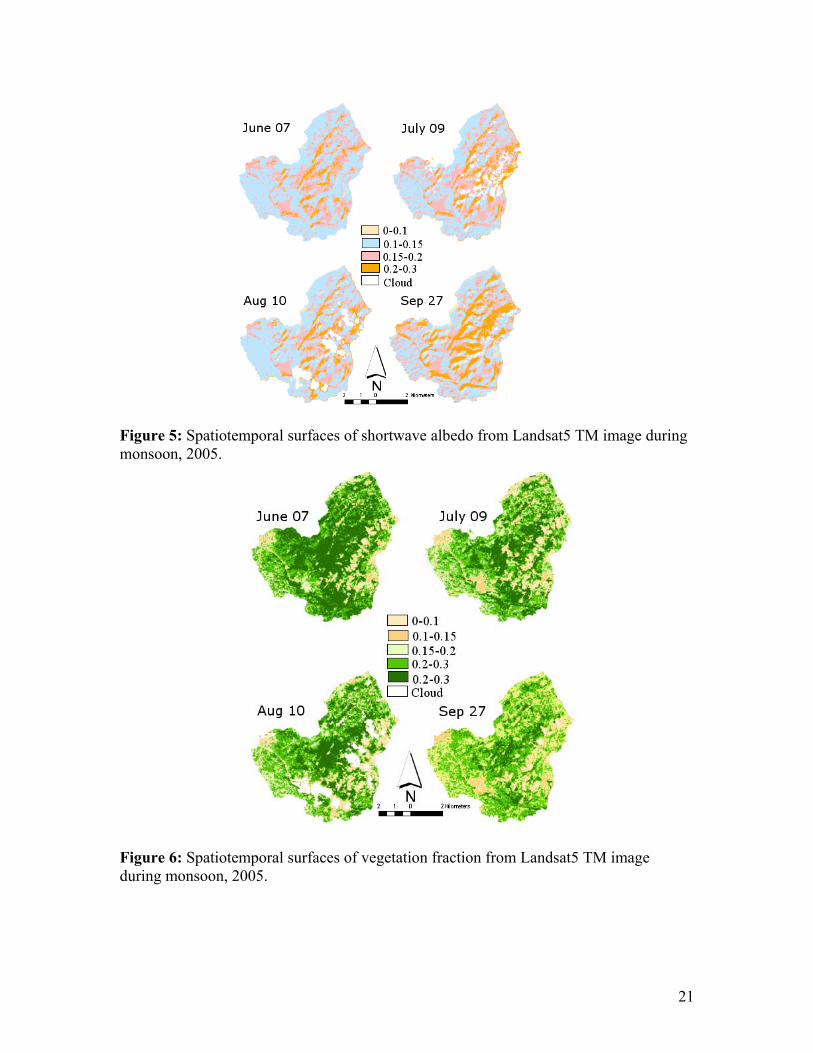
The spatiotemporal surfaces of albedo and vegetation fraction from both Landsat5 TM and MODIS imagery were incorporated in the simulation using dynamic vegetation. The model updated itself with the acquisition of new image. The spatiotemporal albedo from Landsat5 TM shows very little change in vegetation and soil albedo during monsoon, 2005 (Figure 5). However, vegetation decreased significantly during early monsoon (June 7 to July10), which may be attributed to summer temperature and very little rainfall (Figure 6). As the monsoon triggered with a series of precipitation pulses, vegetation fraction increased between the period July and August (Figure 6). The vegetation fraction slightly decreased at the end of the monsoon (Figure 6). 4.1. Soil moisture simulation using static vegetation

4.1.1. Time series comparison

Redondo weather station

Figure 7 shows the comparison between the soil moisture observations at Redondo weather station and the average of simulated soil moisture of the co-located Voronoi polygon and its neighboring Voronoi polygons with 1 standard deviation. During early monsoon, high soil moisture differences are observed between modeled soil moisture and observation due to continuation of snowmelt water inputs into the system (Figure 7). This model version did not account for the snowmelt water in late spring. As the monsoon began, the simulated soil moisture was in good agreement with observed soil moisture. Since late June, good agreement between observed soil moisture and simulated soil moisture are found during rest of the summer period with few exceptions. The tRIBS model successfully captures the observed temporal soil moisture dynamic during both high intensity rainfall event and inter-storm periods. Grassland sites

Figure 8 illustrates the comparison between daily soil moisture observation and modeled soil moisture during the field campaign at grassland sites. Overall, the model captures the observed soil moisture in all grassland sites. However, the model slightly underestimates soil moisture at R5 site (Figure 8D) during the field campaign and at the R4 (Figure 8C) and R2 (Figure 8B) sites during first two days of the field campaign. Forest sites

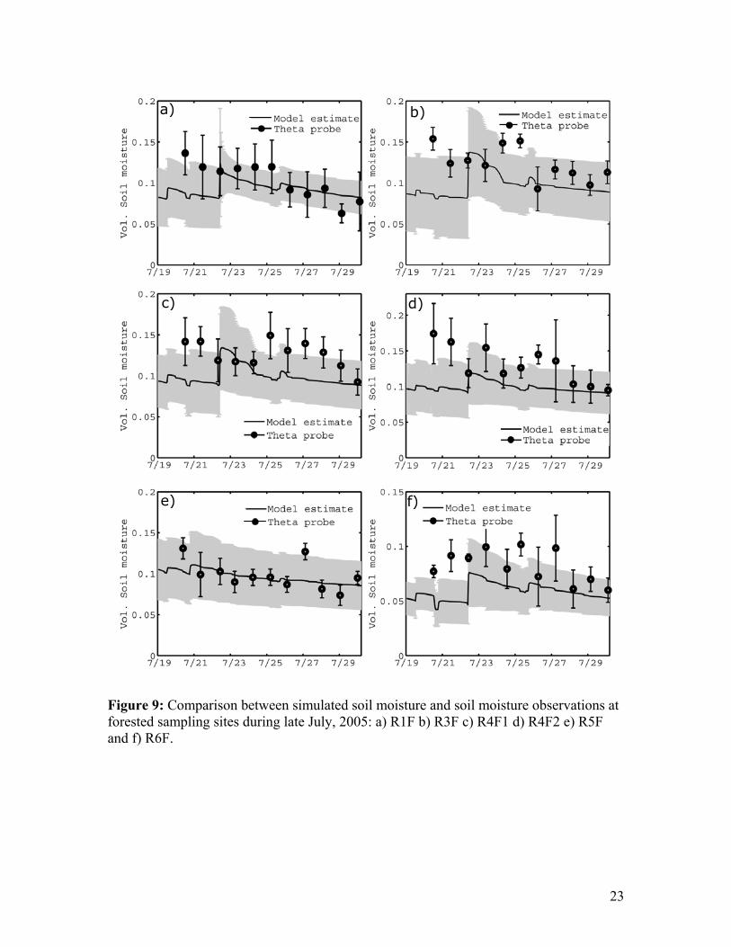
Figure 9 also shows good agreement between the daily soil moisture observation and modeled soil moisture during the field campaign in forest sites. However, simulated soil moisture is slightly underestimated with respect to observation in all forest sites, except R5F. Relatively higher discrepancies between model estimates and observations are prominent during first two days of the field campaign. However, the differences between model estimate and observations reduce significantly after sudden rise of simulated moisture at July 22, due to a precipitation pulse in all forest sites.

11

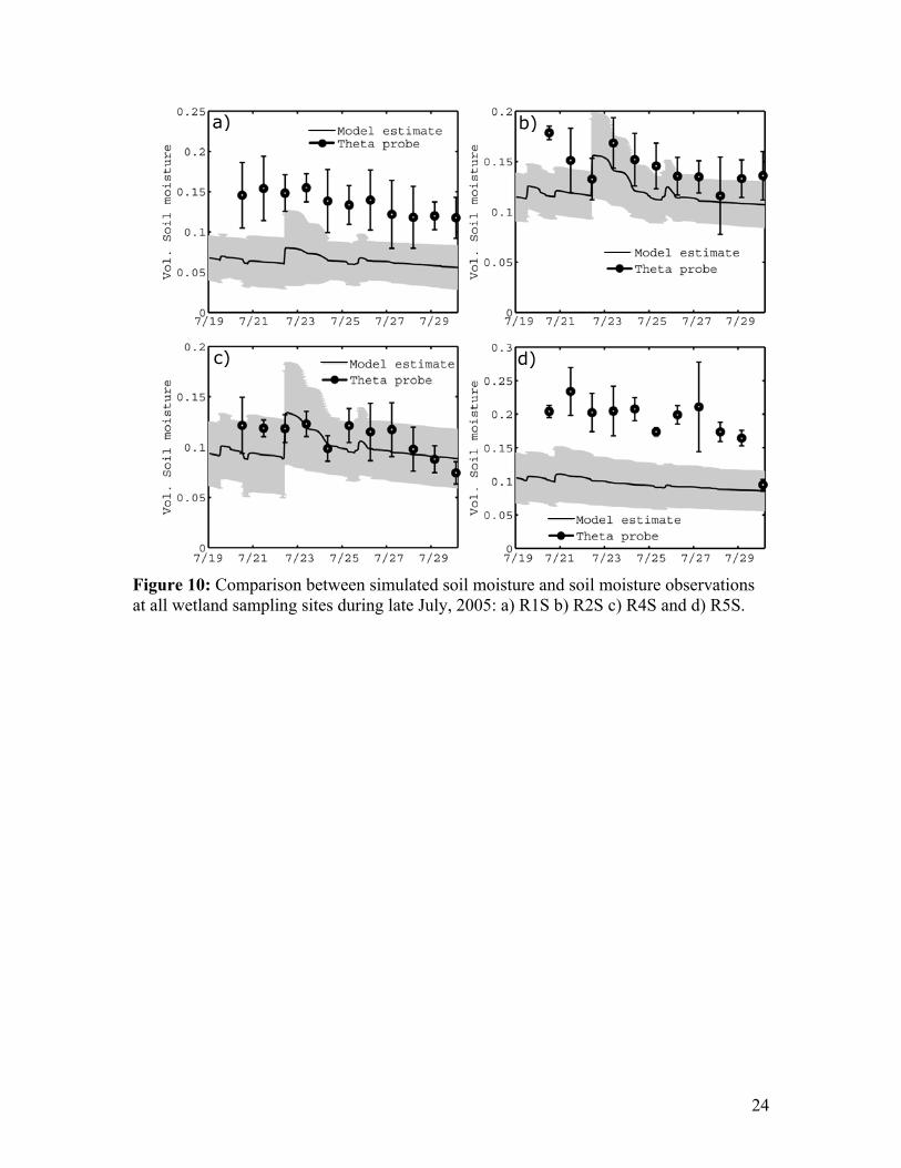
Wetland Relatively higher soil moisture differences are observed in wetland as compared to grassland and forest sites (Figure 10). The model under estimates soil moisture at R1 and R5 site while model predictions are generally in good agreement in R2 and R4 sites. Relatively weak prediction of the model in the wetland site may be attributed to watershed representations. It is challenging to capture low lying saturated zones around a stream due to the lack of vertical resolution of the DEM. 4.1.2. Spatial soil moisture field

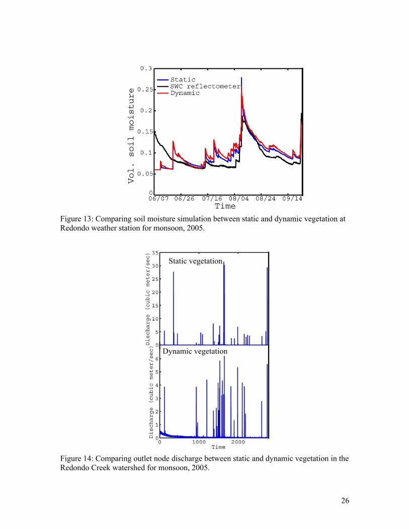
The tRIBS model provides the spatial fields of soil moisture at different times during the monsoon period. Spatial variations of soil hydraulic properties, topography and precipitation influence the spatial soil moisture distribution during simulations. Figure 11 shows the soil moisture field at 12 PM of 9 respective days (2 week temporal interval). During the dry period of the monsoon (Figure 11a, 11b and 11c), the soil moisture spatial distributions are controlled by soil hydraulic properties such as saturated hydraulic conductivity. As a result, soil units with low hydraulic conductivity, such as silty clay and clay loam, contain more moisture than the soil units with high hydraulic conductivity, such as coarse sandy loam and sandy loam. Topography also plays an important role in spatial soil moisture distribution. The areas of flat valleys tend hold more moisture than the areas of hillslopes due to gravity driven lateral and vertical fluxes. As monsoon triggers during late July, spatial variability of precipitation exerts more controls on spatial distributions of soil moisture (Figure 11d and 11e). Soil moisture is relatively high in the central part of the basin due to high precipitation. The entire basin becomes wet during middle August due to high frequency and intensity rainfall events during that time (Figure 11f and 11g). As the system receives more rainfall, the controls of soil properties are less prominent in spatial distribution of soil moisture (Figure 11h and 11i). During the later part of the monsoon (September), the basin dries out due to decrease of the frequency and intensity of precipitation events. 4.2. Comparison between static and dynamic vegetation The current simulation using dynamic vegetation considers only the spatiotemporal variation of albedo and vegetation fraction. Figure 12 shows the comparison between simulated soil moisture using static vegetation and dynamic vegetation at the weather station. During early monsoon, good agreement was observed between simulated soil moisture using static and dynamic vegetation. However, the simulation using dynamic vegetation overestimated soil moisture compared to the simulation using static vegetation during last two week of July 2005. During the peak of the monsoon period (middle August), soil moisture using the dynamic vegetation agrees more with observation than the static vegetation. Dynamic vegetation also impact the basin streamflow response. Figure 13 shows the comparison of outlet node streamflow between simulations using static and dynamic

12

vegetation. The impacts of dynamic vegetation decrease discharge significantly at the outlet node. The discharge using dynamic vegetation seems more realistic than the static vegetation. The remotely sensed vegetation fraction in dynamic vegetation represents higher vegetation fraction than coarse spatial resolution static vegetation. As a result, vegetation fraction using dynamic vegetation intercepts more water and uptakes more water for transpiration, which ultimately lead to less streamflow in the basin. This is a demonstration of the impact of spatiotemporal variation of remotely sensed vegetation fraction on interception, evapotranspiration and streamflow. 5. Conclusions

The following conclusions can be drawn from the current study:

• Remotely sensed imagery such as Landsat5 TM and MODIS are useful data sources for extracting vegetation biophysical parameters such as albedo and vegetation fraction. The extracted vegetation parameters help us to investigate the spatiotemporal vegetation dynamics.

• The tRIBS model efficiently performs the soil moisture simulation using both

static and dynamic vegetation. Using static vegetation, tRIBS model soil moisture estimates are in good agreement with observations at Redondo weather station and other distributed locations during field campaign.

• The simulated results using static vegetation varies from the simulated output

using remotely sensed dynamic vegetation. The outlet node discharge significantly decreases after using remotely sensed dynamic vegetation (albedo and vegetation fraction).

13

References Aber JD, Ollinger SV, Federer CA, Reich PB, Goulden ML, Kicklighter DW, Mellilo JM and Lathrop Jr. RG. 1995. Predicting the effects of climate change on water yield and forest production in the northeastern United States. Climate Research 5: 207-222. Aboal JR, Jimenez MS, Morales D and Gil P. 2000. Effects of thinning on throughfall in Canary Islands pine forest- the role of fog. Journal of Hydrology 238: 218-230. Alves DS. 2002. Space-time dynamics of deforestation in Brazilian Amazõnia. International Journal of Remote Sensing 23(14): 2903-2908. Anderson J, Refsgaard JC and Jensen KH. 2001. Distributed hydrological modeling of the Senegal River Basin – model construction and validation. Journal of Hydrology 247: 200-214. Band BE, Patterson P, Nemani R and Running SW. 1993. Forest ecosystem processes at watershed scale: incorporating hillslope hydrology. Agricultural and Forest Meteorology 63: 93-126. Beven KJ. 1982. On subsurface streamflow: An analysis of response times. Hydrological Sciences Journal 29: 425-434. Beven KJ. 1984. Infiltration into a class of vertically nonuniform soils. Hydrological Sciences Journal 27: 505-521. Bhuttle JM, Creed IF and Pomeroy JW. 2000. Advances in Canadian forest hydrology, 1995-1998. Hydrological Processes 14: 1551-1578. Bosch JM and Hewlett JD. 1982. A review of catchment experiment to determine the effect of vegetation changes in water yield and evapotranspiration. Journal of Hydrology 55: 3-23. Bras RL. 1990. Hydrology: An introduction to hydrologic science. Addison-Wesley-Longman, Reading, Mass. Carter GA. 1998. Reflectance wave bands and indices for remote estimation of photosynthesis and stomatal conductance of Pine canopies. Remote Sensing of Environment 63: 61-72. Childs EC and Bydordi M. 1969. The vertical movement of water in stratified porous material; 1. Infiltration. Water Resources Research 5: 446-459. Choudhury BJ, Ahmed NU, Idso SB, Reginato RJ and Daughtry CST. 1994. Relations between evaporation coefficients and vegetation indices studied by model simulations. Remote Sensing of Environment 50(1): 1-17.

14

Colby JD. 1991. Topographic normalization in rugged terrain. Photogrammetric Engineering and Remote Sensing 57(12): 1745-1753. Coop JD and Givnish TJ. 2007a. Gradient analyses of reversed treelines and grasslands of the Valles Caldera, New Mexico. Journal of Vegetation Science 18(1): 43-54. Coop JD and Givnish TJ. 2007b. Spatial and temporal patterns of recent forest encroachment in montane grasslands of the Valles Caldera, New Mexico, USA. Journal of Biogeography 34: 914-927. Coppin PR and Bauer ME. 1996. Digital change detection in forest ecosystems with remote sensing imagery. Remote Sensing of Environment 13: 207-234. Crockford RH and Richardson DP. 2002. Partitioning rainfall into throughfall, stemflow and interception: effect of forest type, ground cover and climate. Hydrological Processes 14: 2903-2920. Eagleson PS. 2002. Ecohydrology: Darwinian expression of vegetation form and function Cambridge Press. Cambridge, UK. 443 pp. Ellis SR, Levings GW, Carter LF, Richey SF and Radell MJ. 1993. Rio Grande Valley, Colorado, New Mexico and Texas. Water Resources Bulletin 29(4): 617-646. Entekhabi, D. 2000. Land surface processes: Basic tools and concepts. Department of Civil and Environmental Engineering, MIT, Cambridge, MA. Fromento-Trigilio ML and Pazzaglia FJ. 1998. Tectonic geomorphology of the Sierra Nacimiento: Traditional and new techniques in assessing long-term landscape evolution in the southern rocky mountains. Journal of Geology 106: 433-453. Gash JHC, Llyod CR and Lachaud G. 1995. Estimating sparse forest rainfall interception with an analytical model. Journal of Hydrology 170: 79-86. Goff F, Kues BS, Rogers MA, McFadden LD and Gardner JN. 1996. The Jemez Mountains Region New Mexico Geological Society, Forty-Seventh Annual Field Conference. 484 pp. Goff F and Gardner JN. 1994. Evolution of mineralized geothermal system, Valles Caldera, New Mexico. Bulletin of the Society of Economic Geologists 89(8): 1803-1832. Granier A, Huc R and Barigah ST. 1996. Transpiration of natural rain forest and its dependence on climatic factors. Agricultural and Forest Meteorology 78: 19-29. Harr RD. 1977. Water flux in soil and subsoil on a steep forested slope. Journal of Hydrology 33: 37-58.

15

Hedstorm NR and Pomeroy JW. 1988. Measurements and modeling of snow interception in boreal forest. Hydrological Processes 12: 1611-1625. Heiken G, Goff F, Gardner JN, Baldridge WS, Hulen JB, Nielson DL and Vaniman D. 1990. The Valles/Toledo Caldera complex, Jemez volcanic field, New Mexico. Annual Reviews of Earth and Planetary Science Letters 18: 27-53. Hu Z and Islam S. 1995. Prediction of ground surface temperature and soil moisture content by the force-restore method. Water Resource Research 31: 2531-2539. Ivanov VY, Vivoni ER, Bras RL and Entekhabi D. 2004a. Catchment hydrologic response with fully distributed triangulated irregular network model. Water Resources Research 40: W11102, DOI:10.1029/2004WR003218. Ivanov VY, Vivoni ER, Bras RL and Entekhabi D. 2004b. Preserving high-resolution surface and rainfall data in operational-scale basin hydrology; a fully-distributed physically-based approach. Journal of Hydrology 298: 80-111. Ivanov VY, Bras RL and Vivoni ER. 2008. Vegetation-Hydrology Dynamics in Complex Terrain of Semiarid Areas. I A Mechanistic Approach to Modeling Dynamic Feedbacks. Water Resources Research. (In Press). Jensen JR. 1996. Introductory digital image processing a remote sensing perspective Prentice Hall, Upper Saddle River, New Jersey. 316 pp. Lee R. 1980. Forest hydrology. Columbia University Press. New York, USA. 349 pp. Lin JD. 1980. On the force-restore method for prediction of ground surface temperature. Journal of Geophysical Research 85(C6): 3251-3254. Liang, S, Strahler, A and Walthall C. (1999), Retrieval of land surface albedo from satellite observations: a simulation study, Journal of Applied Meteorology, 38: 712-725. Liang S. 2000. Narrow band to broadband conversions of land surface albedo I algorithms. Remote Sensing of Environment 76: 213-238. Monteith JL. 1965. Evaporation and the environment. The state and movement of water in living organisms. Symposium of the Society of Experimental Biologists, XIX. 19: 205-234. Motovilov YJ, Gottschalk L, Engeland K and Rodhe A. 1999. Validation of a distributed hydrologic model against spatial observations. Agricultural and Forest Meteorology 98-99: 257-277. Muldavin E, Neville P, Jackson C and Neville T. 2006. A vegetation map of Valles Caldera National Preserve, New Mexico. Natural Heritage New Mexico. 59 pp.

16

O’Callaghan JF and Mark DM. 1984. The extraction of drainage networks from digital elevation data. Computer Vision and Graphics Image Processing. 28, 323– 344. Penman HL. 1948. Natural evaporation from open water, bare soil and grass. Proceeding of the Royal Society of London, Ser. A 193: 120-145. Rao U, Fehn U, Teng RTD, Goff F. 1996. Sources of chloride in hydrothermal fluids from the Valles Caldera, New Mexico: A CL-36 study. Journal of Volcanology and Geothermal Research 72(1-2): 59-70. Roberts J. 1983. Forest transpiration: a conservative hydrologic process. Journal of Hydrology 66: 133-141. Rutter AJ, Kershaw KA, Robins PC and Morton AJ. 1971. A predictive model of rainfall interception in forests: 1. Derivation of the model from observation in a plantation of Corsican pine. Agricultural Meteorology 9: 367-384. Rutter AJ, Morton AJ and Robins PC. 1975. A predictive model of rainfall interception in forests: 2. Generalization of the model and comparison with observation in some coniferous and hardwood stands. Journal of Applied Ecology 12: 367-380. Sandvig RM and Phillips FM. 2006. Ecohydrological control on soil moisture fluxes in arid to semiarid vadose zone. Water Resources Research 42: W08422. Schultz GA. Remote sensing applications to hydrology: runoff, Hydrological Sciences 41: 453–475. Singh A. 1989. Review article on digital change detection techniques using remotely sensed data. International Journal of Remote Sensing 10(6): 989-1007. Small EE and Kurc SA. 2003. Tight coupling between soil moisture and the surface radiation budget in semiarid environments: Implications for land-atmosphere interactions. Water Resources Research 39(10): Art No. 1278. Smith JL, Lin TL and Ranson KJ. 1980. The lambertian assumption and Landsat data. Photogrammetric Engineering and Remote Sensing 46(9): 1183-1189. Vivoni ER, Ivanov VY, Bras RL and Entekhabi D. 2004.Generation of triangulated irregular networks based on hydrological similarity. ASCE Journal of Hydrological Engineering 9: 288-303. Vivoni ER, Ivanov VY, Bras RL and Entekhabi D. 2005. On the effects of triangulated terrain resolution on distributed hydrologic model response. Hydrological Processes 19: 2101-2122. Vivoni ER, Rinehart AJ, Méndez-Barroso LA, Aragon CA, Bisht G, Cardenas MB, Engle E, Forman BA, Frisbee MD, Gutiérrez-Jurado HA, Hong S, Mahmood TH, Kinwai T and

17

Wyckoff RL. 2008. Vegetation controls on soil moisture distribution in the Valles Caldera New Mexico, during the North American Monsoon. Ecohydrology (submitted).

Western AW, Grayson RB and Green TR. 1999. The Tarrawarra Project: High resolution spatial measurement, modelling and analysis of hydrological response. Hydrological Processes 13: 633-652.

18

Figure 1: (a) Location of map of Jemez River Basin in northern New Mexico. (b) Location map of Redondo Creek Watershed in the Jemez River Basin. (c) Location of USGS stream gauge (1980-1984), sampling plots from July 2005 field campaign (Vivoni et al., 2008) and weather stations (VCNP) in Redondo Creek watershed.

36

º 40

´N

36

º 00

´N

36

º 40

´N

36

º 00

´N

106º 40´W

106º 40´W b) c)

a)

19

Figure 2: (a) High resolution (2 m) Vegetation map (VCNP) of the Redondo Creek Watershed (VCNP). (b) Soil texture map of Redondo creek Watershed (SSURGO).

20

Figure 3: a) Plot of horizontal point density and RMSE between DEM and TIN surface with Zr value. b) Percent change of elevation, slope and convex upward curvature from finest resolution TIN (d=0.9937). Figure 4: Triangulated Irregular Network (TIN) surface using 15 meter Zr value, stream network using 0.5 km2 area using area threshold method and floodplain using 10 meter floodplain height and 3rd order stream.

21

Figure 5: Spatiotemporal surfaces of shortwave albedo from Landsat5 TM image during monsoon, 2005. Figure 6: Spatiotemporal surfaces of vegetation fraction from Landsat5 TM image during monsoon, 2005.

22

Figure 7: Comparison between simulated soil moisture and soil moisture observations at Redondo weather stations during monsoon, 2005. Figure 8: Comparison between simulated soil moisture and soil moisture observations at grassland sampling sites during late July, 2005: a) R1B b) R2B c) R3B and d) R5B.

c) d)

a) b)

23

Figure 9: Comparison between simulated soil moisture and soil moisture observations at forested sampling sites during late July, 2005: a) R1F b) R3F c) R4F1 d) R4F2 e) R5F and f) R6F.

a) b)

c) d)

e) f)

24

Figure 10: Comparison between simulated soil moisture and soil moisture observations at all wetland sampling sites during late July, 2005: a) R1S b) R2S c) R4S and d) R5S.

c) d)

a) b)

25

Figure 11: Spatial simulated soil moisture distribution at 12 PM of following dates: a) Jun 07 b) Jun 20 c) Jul 04 d) Jul 18 e) Aug 01 f) Aug 15 g) Aug 22 h) Aug 29 and i) Sep 12.

a) b) c)

e) f) g)

h) i) j)

26

Figure 13: Comparing soil moisture simulation between static and dynamic vegetation at Redondo weather station for monsoon, 2005. Figure 14: Comparing outlet node discharge between static and dynamic vegetation in the Redondo Creek watershed for monsoon, 2005.

Static vegetation

Dynamic vegetation