IMPACTS OF EXTERNAL PRICE SHOCKS ON MALAYSIAN … · Economic Analysis Working Papers.- 7th Volume...

Economic Analysis Working Papers.- 7th Volume – Number 10

Documentos de Trabajo en Análisis Económico.- Volumen 7 – Número 10

1

IMPACTS OF EXTERNAL PRICE SHOCKS ON MALAYSIAN MACRO ECONOMY-AN APPLIED GENERAL EQUILIBRIUM ANALYSIS Al-Amin*1, Chamhuri Siwar**, & Abdul Hamid*** Abstract This paper examines the impacts of external price shocks in the Malaysian economy. There are three simulations are carried out with different degrees of external shocks using Malaysian Social Accounting Matrix (SAM) and Computable General Equilibrium (CGE) analysis. The model results indicate that the import price shocks, better known as external price shocks by 15% decreases the domestic production of building and construction sector by 25.87%, hotels, restaurants and entertainment sector by 12.04%, industry sector by 12.02%, agriculture sector by 11.01%, and electricity and gas sector by 9.55% from the baseline. On the import side, our simulation results illustrate that as a result of the import price shocks by 15%, imports decreases significantly in all sectors from base level. Among the scenarios, the largest negative impacts goes on industry sectors by 29.67% followed by building and construction sector by 22.42%, hotels, restaurants and entertainment sector by 19.45%, electricity and gas sector by 13.%, agriculture sector by 12.63% and other service sectors by 11.17%. However significant negative impact goes to the investment and fixed capital investment. It also causes the household income, household consumption and household savings down and increases the cost of livings in the economy results in downward social welfare. Resumen

El presente artículo examina los impactos de los precios externos en la economía de Malasia. Se llevaron a cabo tres simulaciones con diferentes grados de impactos externos usando la Matriz de Contabilidad Social de Malasia (por sus siglas en inglés SAM) y el análisis de Equilibrio General Computable (CGE). Los resultados indican que los impactos del precio de importación, conocidos como impactos de precio externo, disminuyen en un 15% la producción nacional, el sector de la construcción en un 25,87%, el sector del entretenimiento, hoteles y restaurantes en un 12,04%, el sector de la industria en un 12,02%, el sector de la agricultura en un 11,01% y el sector del gas y la electricidad en un 9,55% de los valores de referencia. En cuanto a las importaciones, los resultados de nuestra simulación muestran que como consecuencia de los impactos del precio de importación en un 15%, las importaciones descienden significativamente en todos los sectores del nivel base. Por áreas, los mayores impactos negativos inciden en los sectores de la industria en un 29,67%, seguidos del sector de la construcción en un 22,42%, el sector del entretenimiento, hoteles y restaurantes en un 19,45%, el sector del gas y la electricidad en un 13%, el sector de la agricultura en un 12,63% y otros sectores de servicio en un 11,17%. De igual manera, este impacto negativo afecta a la inversión y concretamente a la inversión en capital fijo. Asimismo, bajan los ingresos, el consumo y el ahorro domésticos, incrementando el coste de vida en la economía con el consiguiente recorte de las prestaciones sociales.

*Abul Quasem Al-Amin, PhD Researcher, LESTARI, Universiti Kebangsaan Malaysia, 43600 Bangi, Selangor DE Malaysia. E-mail: [email protected] Tel: +603-8921 4161. ** Chamhuri Siwar, Professor, LESTARI, Universiti Kebangsaan Malaysia, 43600 Bangi, Selangor DE Malaysia. E-mail: [email protected] Tel: + 603-8921 4154. *** Dr. Abdul Hamid Jaafar, Asso. Prof, Faculty of Business and Economics, Universiti Kebangsaan Malaysia, 43600 Bangi, Selangor DE Malaysia. E-mail: [email protected] Tel: + 603-8921 3757. #The research paper prepared for Journal Publication.

1 Corresponding author: e-mail: [email protected] or [email protected]



2

1. Introduction External price shocks, especially oil prices immobile matter to the health of the world economy. Higher oil prices since 1999 – partly the result of OPEC supply-management policies – contributed to the global economic downturn in 2000-2001 and are dampening the current cyclical upturn: world GDP growth may have been at least half a percentage point higher in the last two or three years had prices remained at mid-2004 levels. By March 2004, crude prices were well over $10 per barrel higher than three years before. International oil prices started to increase sharply in 2004 and reached to historically high levels in early June 2008. Current market conditions are more unstable than abnormal, in part because of geopolitical uncertainties and because tight product markets – notably for gasoline in the United States – are reinforcing upward pressures on crude prices. Higher prices are contributing to stubbornly high levels of unemployment and exacerbating budget-deficit problems in many OECD, Non-OECD and other oil-importing countries. The adverse economic impact of higher external shocks of oil prices on oil-importing developing countries is generally even more severe than for OECD countries. This is because their economies are more dependent on imported oil and more energy-intensive, and because energy is used less efficiently. Developing countries are also less able to weather the financial turmoil wrought by higher oil-import costs. On average, oil-importing developing countries such as Malaysia, use more than twice as much oil to produce a unit of economic output as do OECD countries. There are several studies addressed the role of trade and external prices shocks (especially oil price shocks) in determining the extent recession, macroeconomic instability and real business cycle, exports-imports magnitude, causality and asymmetric macroeconomic responses caused by the oil price shocks (Rasche and Tatom’s 1977, 1981; Darby 1982; Bruno and Sachs 1982, 1985; Hamilton 1983; Griffin 1985; Mork 1989; Wirl 1990; Dahl and Yucel 1991; Eastwood’s 1992; Mork’s 1994; Mork et al. 1994; Hamilton 1996; Backus et al. 2000; Barsky et al. 2002; Hamilton et al. 2004; Fiorella de Fiore et al. 2006). However the methodologies employed in those studies are varied and so are their results but it is evident that external price shocks extent recession unless appropriate trade policy is in place. Several studies have given a detailed evaluation of import price shocks in the world economy, but little attention has been applied to inquiring about these relationships in the Asian newly industrialized and highly export-oriented countries (so called NICs2) such as Malaysia.

The high and rising oil prices in the international market are affecting the Malaysian economy, through its effect on the balance of payments (BOP) and on domestic prices through various channels. As fuel and food are core elements in Malaysian household budgets, higher fuel prices as a result of external shocks along with other price increases reduced disposable income and social welfare. Increased cost of doing business and margin compression would erode producers’ profits and may cause them to cut back on output. CIMB (2008) partially estimates lower for private consumption growth to 6.3% in 2008 (from 7% previously) and 5.5% in 2009 (10.8% in 2007) and for private investment growth to 6.5% in 2008 (from 7.1% previously) and will be 6.6% in 2009 (12.3% in 2007). There are very essential to estimate of other measurable impact on the broad sectors of the economy such as transportation and logistic industry, food retailers, traders, construction, economic imports, household income and consumption, household savings, enterprise savings, total economic investment, and other related GDP variables indeed. Therefore, the principle focus of this study is to show empirically the impact of external price shocks on macroeconomic indicators such as on domestic production, imports, household income and consumption, household savings, enterprise savings, total economic investment, and other GDP related variables and their different magnitudes of different degrees of external shocks.

2 NISc means newly industrialized countries



3

The paper is organized as follows. A literature with background is summarized in section 1. In section 2, we present the underlying model, which is based on Computable General Equilibrium (CGE) techniques. Simulation results are carried out in Section 3. The discussions with policy recommendations are given in Section 4 and Appendix A is a presentation of the Malaysian computable general equilibrium model in complete equation form.

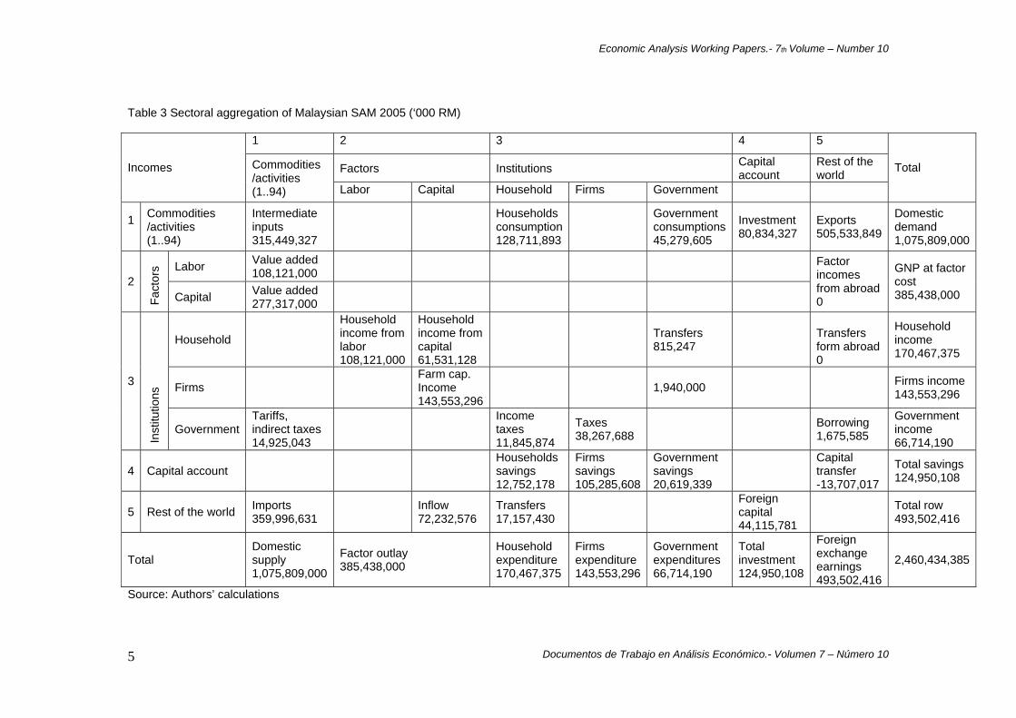
2. Methodology A static computable general equilibrium (CGE) model of the Malaysian economy is constructed for this study. The model consists of ten industries, one representative household, three factor production, and rest of the world. The CGE technique is an approach that tries to develop one of the fundamental concepts of economics, namely to grasp the complex interdependent relationships among decentralized actors in an economy by considering the actual outcome to represent a ‘general equilibrium’. More compactly, the technique expresses that the ‘equilibrium’ of an economy is reached when expenditures by consumers exactly exhaust their disposable income, the aggregate value of exports exactly equals import demand, and the cost of pollution is just equal at the margin of the social value of damage that it causes. The benchmark model representing the baseline economy is constructed using a Social Accounting Matrix (SAM)3. A SAM is a snapshot and code database for CGE analysis that reflecting monetary flow of interactions among institutions in the Malaysian full economy which is shown in Table 3. The Malaysian CGE model is presented in this section, which is a set of non-linear simultaneous equations followed by Dervis et al (1982) and Robinson et al (1999) model; where the number of equations is equal to the number of endogenous variables. This section introduces the framework of the CGE model and algorithm for solving the objectives. The equations are classified in four different blocks, such as price, production, institutions and system constraints are presented as follows.

3 SAM matrix is estimated by the Authors using the Malaysian updated 2000 input-output table and national accounts Malaysia 2005 (DOS, 2005). For more details of aggregated SAM see Table 3.



4

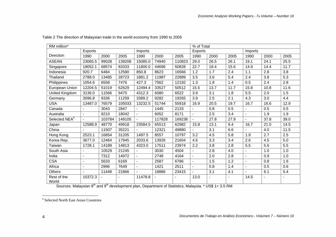
Table 2 The direction of Malaysian trade in the world economy from 1990 to 2005

RM million* % of Total Exports Imports Exports Imports

Direction 1990 2000 2005 1990 2000 2005 1990 2000 2005 1990 2000 2005 ASEAN 23065.5 99028 139208 15085.0 74940 110823 29.0 26.5 26.1 19.1 24.1 25.5 Singapore 18052.1 68574 83333 11800.0 44696 50828 22.7 18.4 15.6 14.9 14.4 11.7 Indonesia 920.7 6484 12580 850.8 8623 16566 1.2 1.7 2.4 1.1 2.8 3.8 Thailand 2788.0 13485 28723 1881.2 11987 22889 3.5 3.6 5.4 2.4 3.8 5.3 Philippines 1054.6 6558 7476 427.3 7562 12192 1.3 1.8 1.4 0.5 2.4 2.8 European Union 12204.5 51019 62629 12494.4 33527 50512 15.5 13.7 11.7 15.8 10.8 11.6 United Kingdom 3136.0 11566 9470 4312.3 6080 6522 3.9 3.1 1.8 5.5 2.0 1.5 Germany 3096.8 9336 11259 3389.2 9282 19265 3.9 2.5 2.1 4.3 3.0 4.4 USA 13487.0 76579 105033 13232.5 51744 55918 16.9 20.5 19.7 16.7 16.6 12.9 Canada - 3043 2847 - 1445 2133 - 0.8 0.5 - 0.5 0.5 Australia - 9210 18042 - 6052 8171 - 2.5 3.4 - 1.9 1.9 Selected NEA4 - 103784 149105 - 117828 169236 - 27.8 27.9 - 37.8 39.0 Japan 12588.9 48770 49918 23584.5 65513 62982 15.8 13.1 9.4 16.7 21.0 14.5 China - 11507 35221 - 12321 49880 - 3.1 6.6 - 4.0 11.5 Hong Kong 2523.1 16854 31205 1497.5 8557 10797 3.2 4.5 5.8 1.9 2.7 2.5 Korea Rep. 3677.0 12464 17945 2033.6 13926 21604 4.6 3.3 3.4 2.6 4.5 5.0 Taiwan 1728.1 14189 14813 4323.0 17511 23974 2.2 3.8 2.8 5.5 5.6 5.5 South Asia - 10529 21245 - 3030 4504 - 2.8 4.0 - 1.0 1.0 India - 7312 14972 - 2748 4164 - 2.0 2.8 - 0.9 1.0 CSA - 5633 6169 - 2587 6786 - 1.5 1.2 - 0.8 1.6 Africa - 2996 7649 - 1421 2511 - 0.8 1.4 - 0.5 0.6 Others - 11449 21866 - 18886 23415 - 3.1 4.1 - 6.1 5.4 Rest of the World

10372.3 - - 11478.8 - - 13.0 - - 14.5 - -

Sources: Malaysian 8th and 9th development plan, Department of Statistics, Malaysia. * US$ 1= 3.5 RM

4 Selected North East Asian Countries



5

Table 3 Sectoral aggregation of Malaysian SAM 2005 (‘000 RM)

1 2 3 4 5

Factors Institutions Capital account

Rest of the world Incomes Commodities

/activities (1..94) Labor Capital Household Firms Government

Total

1

Commodities /activities (1..94)

Intermediate inputs 315,449,327

Households consumption 128,711,893

Government consumptions45,279,605

Investment 80,834,327

Exports 505,533,849

Domestic demand 1,075,809,000

Labor Value added 108,121,000

2

Fact

ors

Capital Value added 277,317,000

Factor incomes from abroad 0

GNP at factor cost 385,438,000

Household

Household income from labor 108,121,000

Household income from capital 61,531,128

Transfers 815,247

Transfers form abroad 0

Household income 170,467,375

Firms Farm cap. Income 143,553,296

1,940,000

Firms income 143,553,296

3

Inst

itutio

ns

Government Tariffs, indirect taxes 14,925,043

Income taxes 11,845,874

Taxes 38,267,688 Borrowing

1,675,585

Government income 66,714,190

4 Capital account Households savings 12,752,178

Firms savings 105,285,608

Government savings 20,619,339

Capital transfer -13,707,017

Total savings 124,950,108

5 Rest of the world Imports 359,996,631 Inflow

72,232,576 Transfers 17,157,430

Foreign capital 44,115,781

Total row 493,502,416

Total Domestic supply 1,075,809,000

Factor outlay 385,438,000

Household expenditure 170,467,375

Firms expenditure 143,553,296

Government expenditures 66,714,190

Total investment 124,950,108

Foreign exchange earnings 493,502,416

2,460,434,385

Source: Authors’ calculations



6

2.1 Price block Import price Domestic price of import goods iPM is the tariff, itm induced market price times exchange

rate, ER can be expressed as:

(1 ).i i iPM pwm tm ER= + (1) where, ipwm is the world price of import goods by sector. Export price Export price of export goods iPE is the export tax induced international market price times

exchange rate ER as:

(1 ).i i iPE pwe te ER= − (2)

where, ite export tax rate of export goods by sector, and ipwe is the world price of export goods by sector. Composite price The composite price iP is the price paid by the domestic demanders, can be specified as:

i i i ii

i

PD D PM MPQ

⎛ ⎞+= ⎜ ⎟⎝ ⎠

(3)

where, iD and iM are the quantity of domestic and imported goods respectively, and iPD is the

price of domestically produced goods sold in the domestic market, iPM is the price of imported

goods, and iQ is the composite goods. Activity price The sales or activity price iPX is composed of domestic price of domestic sales and the domestic price of exports can be expressed as:

. .i i i ii

i

PD D PE EPXX+

= (4)

where, iX stands for sectoral output. Value added price Value added price iPV is defined as residual of gross revenue adjusted for taxes and intermediate input costs, is specified as:



7

. (1 ) .i i i i i

ii

PX X tx PK INPVVA− −

= (5)

where, itx is defined as tax per activity and iIN stands for total intermediate input, iPK stands

for composite intermediate input price and iVA stands for value added. Composite intermediate input price Composite intermediate input price iPK is defined as composite commodity price times input-output coefficients.

.i ij jj

PK a P=∑ (6)

where, ija is the input-output coefficient matrix. Numeraire price index In computable general equilibrium model, the system can only determine relative prices, and solves for prices relative to a numeraire. In this model the numeraire is the gross national price deflator (gross domestic product can be used). Producer price index and CPI are also commonly used as numeraire in applied CGE studies. In this model:

GDPVAPPRGDP

= (7)

where, PP is GDP deflator, GDPVA is the GDP at value added price, and RGDP is the real GDP. 2.2 Production block This block contains quantity equations, which describe the supply side of the model. The fundamental form must satisfy certain restrictions of general equilibrium theory. This block define production technology and demand for factors as well as CET transformation functions combining exports and domestic sales, export supply functions and import demand and CES aggregation functions as follows5: D if

i i f ifX a FDSCα= ∏ (8) where, ifFDSC indicates sectoral capital stock and D

ia represents the production function shift parameter by sector. On the other, the next equation expresses first order conditions for profit maximization as follows:

5 The production function here is nested. At the top level, output is a fixed coefficients function of real world value added and intermediate inputs. Real value added is a Cobb-Douglas function of capital and labor. Intermediate inputs are required according to fixed input-output coefficients and each intermediate input is a CES aggregation of imported and domestic goods.



8

. . if if i if

if

XWF wfdist PVFDSC

α= (9)

where, ifwfdist represents sector- specific distortions in factor markets, fWF indicates average

rental or wage, ifα indicates factor share parameter-production function and PV represents the value added price. Intermediate inputs iIN are the function of domestic production can be defined as follows:

.i ij jj

IN a X=∑ (10)

where ija indicates input-output coefficients. On the other, the CET transformation function combining exports and domestic sales can be defined as:

1

[ (1 ) ]T T Ti i iT

i i i i i iX a E Dρ ρ ργ γ= + − (11)

where, iX indicates the sectoral domestic sales, Tia is the CET function shift parameter by

sector, iγ holds the sectoral CET function share parameter, iE is the export demand constant by

sector and T

iρ is the production function of elasticity of substitution by sector. The export supply functions, which depend on relation price (Pe/Pd) can be expressed in the following function:

1/(1 )

.

Tie

i idi i

i i

PE D P

ργ

γ⎡ ⎤−= ⎢ ⎥⎣ ⎦

(12)

Likewise, the world export demand function for sectors in an economy, iecon is assumed

to have some power can be expressed as follows:

i

ii i

i

pweE econ pwseη

⎡ ⎤= ⎢ ⎥⎣ ⎦ (13)

where, ipwse represents the sectoral world price of export substitutes and iη is the CET function exponent by sector.

On the other, composite goods supply describes how imports and domestic product are demanded can be defined as:

1

(1 )C C Ci i iC

i i i i i iQ a M Dρ ρ ρδ δ−

− −⎡ ⎤= + −⎣ ⎦ (14)

where, Cia indicates sectoral armington function shift parameter, and iδ indicates the sectoral

armington function share parameter.

Lastly, the import demand function which depends on relative price (Pd/Pm) can be expressed as follows:



9

11.

(1 )

Ci

di i

mi ii i

PM D Pρδ

δ+⎡ ⎤= ⎢ ⎥−⎣ ⎦

(15)

2.3 Domestic institution block This block consists the equations that map the flow of income from value added to institutions and ultimately to households. These equations fill out the inter-institutional entries in the SAM defined as:

. .Ff f if if

i

Y WF FDSC wfdist=∑ (16)

where, FfY defines factor incomes, which in turn are distributed to capital and labor households

equations, ifFDSC indicates sectoral capital stock, ifwfdist represents sector- specific

distortions in factor markets and fWF indicates average rental or wage. The household factor income from capital can be defined as follows:

1H F

capehY Y DEPREC= − (17)

where, HcapehY indicates the households income from capital, 1

FY represents capital factor income and DEPREC indicates depreciations of capital.

Similarly households labor income, HlabehY defines as:

1

H Flabeh f

fY Y

≠

= ∑ (18)

where, FfY indicates the factor incomes.

On the other hand, tariff equation TARIFF can be expressed as follow: . . .i i i

iTARIFF pwm M tm ER=∑ (19)

Similarly, the indirect tax INDTAX is defined as:

. .i i ii

INDTAX PX X tx=∑ (20)

Likewise, household income tax is expressed as: . ,H H

h hh

HHTAX Y t h cap lab= =∑ (21)

where, HhY indicates households income, H

ht represents income tax rate.

On the other, the export revenue (subsidy) EXPSUB can be expressed as:



10

. . .i i ii

EXPSUB pwe E te ER=∑ (22)

Whereas the total government revenue (GR) is obtained as the sum up the previous four equations as: *GR TARIFF INDTAX HHTAX EXPSUB= + + + (23) * the sign of EXPSUB depends on the economic policy whether government taking export tax or giving subsidies.

The depreciation (DEPREC) is the function of capital stock can be defined as:

. .ii i

iDEPREC depr PK FDSC=∑ (24)

where, idepr represents the sectoral depreciation rates.

On the other, household savings (HHSAV) is a function of marginal propensity to save and income can be expressed as: .(1 ).H H

h h hh

HHSAV Y t mps= −∑ (25)

where, hmps indicates marginal propensity to save.

Likewise government savings (GOVSAV) is a function of GR and final demand for government consumptions can be defined as follows:

.i ii

GOVSAV GR P GD= −∑ (26)

where, iGD represents final demand of government consumptions.

Lastly, the components of total savings include financial depreciation, household savings, government savings and foreign savings in domestic currency (FSAV.ER)

.SAVING HHSAV GOVSAV DEPREP FSAV ER= + + + (27)

The following section provides equations that complete the circular flow in the economy, determining the demand for goods by various actors. First, the private consumption (CD) is obtained by the following assignments:

. .(1 ).(1 ) /H H Hi ih h h h ih

CD Y mps t Pβ⎡ ⎤= − −⎣ ⎦∑ (28)

where, H

ihβ indicates the sectoral household consumption expenditure shares. Likewise, the government demand for final goods (GD) is defined using fixed shares of

aggregate real spending on goods and services (gdtot) as follows:

.Gi iGD gdtotβ= (29)

where, Giβ express sectoral government expenditures.



11

Inventory demand (DST) or change in stock is determined using the following equation as follows:

.i i iDST dstr X= (30)

where idstr indicates the sectoral production shares.

On the other, aggregate nominal fixed investment (FXDINV) is estimated as total investment (INVEST) minus inventory accumulation as:

.i ii

FXDINV INVEST P DST= −∑ (31)

The sector of destination (DK) is calculated from aggregated fixed investment and fixed nominal shares, ikshr using the following function:

. /i i iDK kshr FXDINV PK= (32)

The next equation translates investment by sector of destination into demand for capital goods by sector of origin (ID) using the capital composition matrix, ijb as:

.i ij j

jID b DK=∑ (33)

Lastly the two equations show the nominal and real GDP, which are used to calculate the GDP deflator specific as numeraire in the price equations. Real GDP (RGDP) is defined from expenditure side and nominal GDP (GDPVA) is generated from value added side as follows:

.i ii

GDPVA PV X INDTAX TARIFF EXPSUB= + + +∑ (34)

( ). .i i i i i i ii

RGDP CD GD ID DST E pwm M ER= + + + + −∑ (35)

2.4 Systems constraints block This block defines the constraints that are satisfied by the economy as a whole without being considered by its individual agents. The model’s micro constraints apply to individual markets for factors and commodities. With the few exceptions (for labor, exports, and imports), it is assumed that flexible prices clear the markets for all commodities and factors. The macro constraints apply to the government, the savings-investment balance, and the rest of the world. For the government, savings clear the balance, whereas the investment value adjusts to changes in the value of total savings. For the rest of the world, the alternatives of a fixed exchange rate or flexible foreign savings are permitted in the current formulation. Product market equilibrium condition requires that total demand for composite goods ( iQ ) is equal to its total supply as:

i i i i i iQ IN CD GD ID DST= + + + + (36) Market clearing requires that total factor demand equal total factor supply and the equilibrating variables are the average factor prices which defined earlier and this condition can be expressed as follows:



12

if fi

FDSC fs=∑ (37)

The following equation is the balance of payments represents the simplest evidence form: foreign savings (FSAV) is the difference between total imports and total exports. As foreign savings set exogenously, the equilibrating variable for this equation is the exchange rate (ER). Equilibrium will be achieved through movements in ER that effect export import price. This balancing equation can be expressed as:

. .i i i ipwm M pwe E FSAV= + (38)

Lastly the macro-closure rule is given as:

SAVING INVEST= (39) where total investment adjusts to equilibrate with total savings to bring the economy into the equilibrium. 2.5 Database: Social accounting matrix of Malaysia The model is based on a social accounting matrix (SAM) of information system that provides initial information on the structure and composition of production, the sectoral value added and the distribution of value added among factors of production and households. The updated Input-Output (I-O) table (94x94) of the year 2005 provides the principal data for SAM and main data source for CGE calibrations. The adopted Input-Output table is a transaction table of intermediate inputs grouped by commodity by commodity at producer prices. The parameter values on the other are obtained in such a way that the model’s solution for the base year is capable of same reproducing the assembled equilibrium data in the SAM. By imposing this restriction, the parameter values have been determined from outside the SAM manner of the model’s solution for the base year. Before doing so, the sectoral classification of the I-O table is redesigned for SAM 2005 to confirm the desired estimation and policy formulation. After some adjustments for balancing the 102x102 SAM are aggregated to 17x17 sectors, among which 10 are production sectors. Table 3 presents the aggregated SAM of the Malaysian Economy. 3. Results and discussion 3.1 Effects of import price shocks on Malaysian economy The simulations carried out are based on SAM of the Malaysian economy and the experimental scenario codes and simulation experiments for this study are listed in Table 4. The scenario 1 represents the world price shocks, namely an increase in import prices in the international market. In this simulation the study finds some macroeconomic impacts on Malaysia. These simulations are carried out in three steps such as 1a, 1b and 1c and which represents 5%, 10% and 15% increase in external shocks respectively with trade policy. The simulation effects of import price shocks on domestic production are presented in Table 5. A rise of import prices causes depreciates the real exchange rate that makes import goods expensive in the domestic market. As a result, the demand for imported intermediate input falls and the domestic production decreases. In the Malaysian case, the increase of imports price also fall the domestic output in almost all scenarios.



13

Table 4 scenario codes and definition of the simulations

Scenario codes Simulation specifications

Scen 1a 5 % increase in world market price of import goods+ current

t d liScen 1b 10% increase in world market price of import goods+ current

lib li ti

Scenario 1

Scen 1c 15% increase in world market price of import goods + current

trade policy & existing trade liberalization Theoretically an increase of import prices deteriorates the terms of trade, import contracts most importantly prices of import goods of domestic market increase. More compactly, it means that import goods are more expensive and production and employment may contract causing a fall in household’s income. Consumers can afford less quantity of both domestic and imported goods. Government revenue and savings also falls.

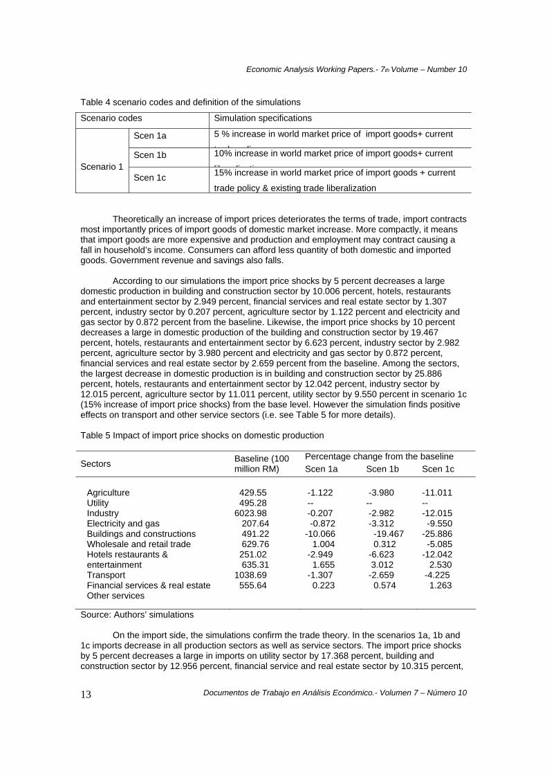
According to our simulations the import price shocks by 5 percent decreases a large domestic production in building and construction sector by 10.006 percent, hotels, restaurants and entertainment sector by 2.949 percent, financial services and real estate sector by 1.307 percent, industry sector by 0.207 percent, agriculture sector by 1.122 percent and electricity and gas sector by 0.872 percent from the baseline. Likewise, the import price shocks by 10 percent decreases a large in domestic production of the building and construction sector by 19.467 percent, hotels, restaurants and entertainment sector by 6.623 percent, industry sector by 2.982 percent, agriculture sector by 3.980 percent and electricity and gas sector by 0.872 percent, financial services and real estate sector by 2.659 percent from the baseline. Among the sectors, the largest decrease in domestic production is in building and construction sector by 25.886 percent, hotels, restaurants and entertainment sector by 12.042 percent, industry sector by 12.015 percent, agriculture sector by 11.011 percent, utility sector by 9.550 percent in scenario 1c (15% increase of import price shocks) from the base level. However the simulation finds positive effects on transport and other service sectors (i.e. see Table 5 for more details). Table 5 Impact of import price shocks on domestic production

Percentage change from the baseline Sectors Baseline (100

million RM) Scen 1a Scen 1b Scen 1c Agriculture Utility Industry Electricity and gas Buildings and constructions Wholesale and retail trade Hotels restaurants & entertainment Transport Financial services & real estate Other services

429.55 495.28 6023.98 207.64 491.22 629.76 251.02 635.31 1038.69 555.64

-1.122 -- -0.207 -0.872 -10.066 1.004 -2.949 1.655 -1.307 0.223

-3.980 -- -2.982 -3.312 -19.467 0.312 -6.623 3.012 -2.659 0.574

-11.011 -- -12.015 -9.550 -25.886 -5.085 -12.042 2.530 -4.225 1.263

Source: Authors’ simulations

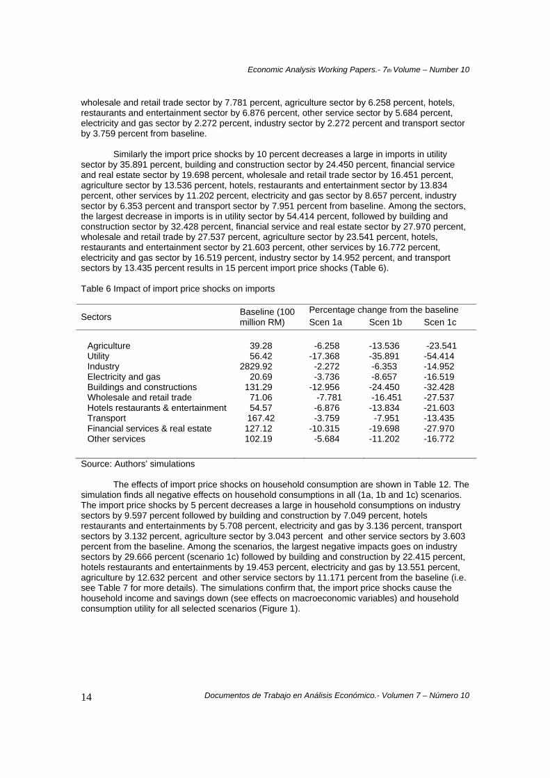
On the import side, the simulations confirm the trade theory. In the scenarios 1a, 1b and 1c imports decrease in all production sectors as well as service sectors. The import price shocks by 5 percent decreases a large in imports on utility sector by 17.368 percent, building and construction sector by 12.956 percent, financial service and real estate sector by 10.315 percent,



14

wholesale and retail trade sector by 7.781 percent, agriculture sector by 6.258 percent, hotels, restaurants and entertainment sector by 6.876 percent, other service sector by 5.684 percent, electricity and gas sector by 2.272 percent, industry sector by 2.272 percent and transport sector by 3.759 percent from baseline.

Similarly the import price shocks by 10 percent decreases a large in imports in utility

sector by 35.891 percent, building and construction sector by 24.450 percent, financial service and real estate sector by 19.698 percent, wholesale and retail trade sector by 16.451 percent, agriculture sector by 13.536 percent, hotels, restaurants and entertainment sector by 13.834 percent, other services by 11.202 percent, electricity and gas sector by 8.657 percent, industry sector by 6.353 percent and transport sector by 7.951 percent from baseline. Among the sectors, the largest decrease in imports is in utility sector by 54.414 percent, followed by building and construction sector by 32.428 percent, financial service and real estate sector by 27.970 percent, wholesale and retail trade by 27.537 percent, agriculture sector by 23.541 percent, hotels, restaurants and entertainment sector by 21.603 percent, other services by 16.772 percent, electricity and gas sector by 16.519 percent, industry sector by 14.952 percent, and transport sectors by 13.435 percent results in 15 percent import price shocks (Table 6). Table 6 Impact of import price shocks on imports

Percentage change from the baseline

Sectors Baseline (100 million RM) Scen 1a Scen 1b Scen 1c

Agriculture Utility Industry Electricity and gas Buildings and constructions Wholesale and retail trade Hotels restaurants & entertainment Transport Financial services & real estate Other services

39.28 56.42 2829.92 20.69 131.29 71.06 54.57 167.42 127.12 102.19

-6.258 -17.368 -2.272 -3.736 -12.956 -7.781 -6.876 -3.759 -10.315 -5.684

-13.536 -35.891 -6.353 -8.657 -24.450 -16.451 -13.834 -7.951 -19.698 -11.202

-23.541 -54.414 -14.952 -16.519 -32.428 -27.537 -21.603 -13.435 -27.970 -16.772


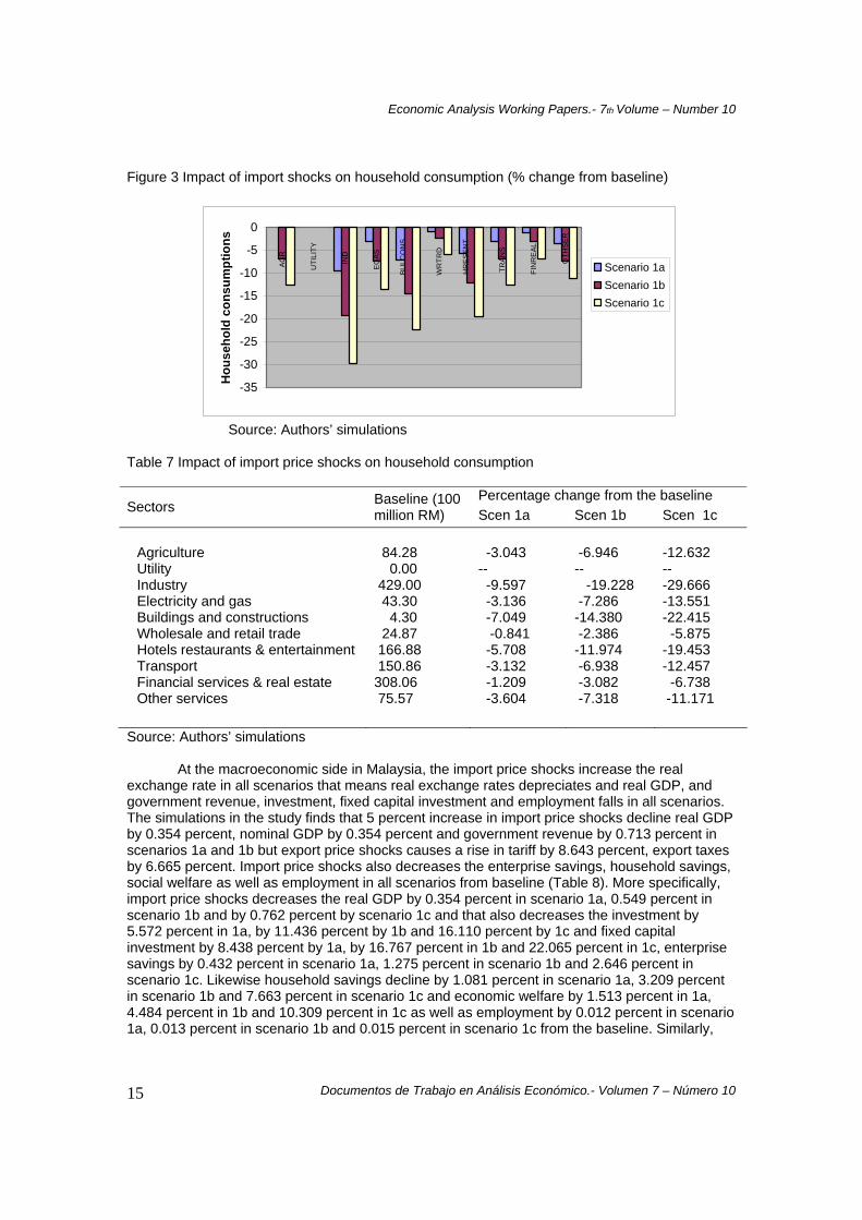
The effects of import price shocks on household consumption are shown in Table 12. The simulation finds all negative effects on household consumptions in all (1a, 1b and 1c) scenarios. The import price shocks by 5 percent decreases a large in household consumptions on industry sectors by 9.597 percent followed by building and construction by 7.049 percent, hotels restaurants and entertainments by 5.708 percent, electricity and gas by 3.136 percent, transport sectors by 3.132 percent, agriculture sector by 3.043 percent and other service sectors by 3.603 percent from the baseline. Among the scenarios, the largest negative impacts goes on industry sectors by 29.666 percent (scenario 1c) followed by building and construction by 22.415 percent, hotels restaurants and entertainments by 19.453 percent, electricity and gas by 13.551 percent, agriculture by 12.632 percent and other service sectors by 11.171 percent from the baseline (i.e. see Table 7 for more details). The simulations confirm that, the import price shocks cause the household income and savings down (see effects on macroeconomic variables) and household consumption utility for all selected scenarios (Figure 1).



15

Figure 3 Impact of import shocks on household consumption (% change from baseline)

-35

-30

-25

-20

-15

-10

-5

0

AGR

UTI

LITY

IND

EG

AS

BULC

ON

S

WR

TRD

HR

ESE

NT

TRAN

S

FIN

RE

AL

OTH

SER

Hou

seho

ld c

onsu

mpt

ions

Scenario 1aScenario 1bScenario 1c


Table 7 Impact of import price shocks on household consumption


million RM) Scen 1a Scen 1b Scen 1c

Agriculture Utility Industry Electricity and gas Buildings and constructions Wholesale and retail trade Hotels restaurants & entertainment Transport Financial services & real estate Other services

84.28 0.00 429.00 43.30 4.30 24.87 166.88 150.86 308.06 75.57

-3.043 -- -9.597 -3.136 -7.049 -0.841 -5.708 -3.132 -1.209 -3.604

-6.946 -- -19.228 -7.286 -14.380 -2.386 -11.974 -6.938 -3.082 -7.318

-12.632 -- -29.666 -13.551 -22.415 -5.875 -19.453 -12.457 -6.738 -11.171

Source: Authors’ simulations At the macroeconomic side in Malaysia, the import price shocks increase the real

exchange rate in all scenarios that means real exchange rates depreciates and real GDP, and government revenue, investment, fixed capital investment and employment falls in all scenarios. The simulations in the study finds that 5 percent increase in import price shocks decline real GDP by 0.354 percent, nominal GDP by 0.354 percent and government revenue by 0.713 percent in scenarios 1a and 1b but export price shocks causes a rise in tariff by 8.643 percent, export taxes by 6.665 percent. Import price shocks also decreases the enterprise savings, household savings, social welfare as well as employment in all scenarios from baseline (Table 8). More specifically, import price shocks decreases the real GDP by 0.354 percent in scenario 1a, 0.549 percent in scenario 1b and by 0.762 percent by scenario 1c and that also decreases the investment by 5.572 percent in 1a, by 11.436 percent by 1b and 16.110 percent by 1c and fixed capital investment by 8.438 percent by 1a, by 16.767 percent in 1b and 22.065 percent in 1c, enterprise savings by 0.432 percent in scenario 1a, 1.275 percent in scenario 1b and 2.646 percent in scenario 1c. Likewise household savings decline by 1.081 percent in scenario 1a, 3.209 percent in scenario 1b and 7.663 percent in scenario 1c and economic welfare by 1.513 percent in 1a, 4.484 percent in 1b and 10.309 percent in 1c as well as employment by 0.012 percent in scenario 1a, 0.013 percent in scenario 1b and 0.015 percent in scenario 1c from the baseline. Similarly,



16

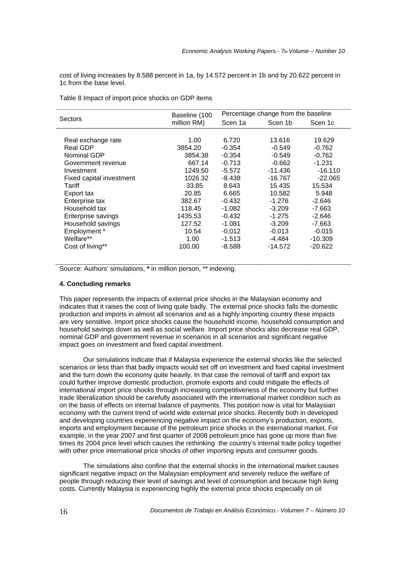
cost of living increases by 8.588 percent in 1a, by 14.572 percent in 1b and by 20.622 percent in 1c from the base level. Table 8 Impact of import price shocks on GDP items


million RM) Scen 1a Scen 1b Scen 1c Real exchange rate Real GDP Nominal GDP Government revenue Investment Fixed capital investment Tariff Export tax Enterprise tax Household tax Enterprise savings Household savings Employment * Welfare** Cost of living**

1.00 3854.20 3854.38 667.14 1249.50 1026.32 33.85 20.85 382.67 118.45 1435.53 127.52 10.54 1.00 100.00

6.720 -0.354 -0.354 -0.713 -5.572 -8.438 8.643 6.665 -0.432 -1.082 -0.432 -1.081 -0.012 -1.513 -8.588

13.616 -0.549 -0.549 -0.662 -11.436 -16.767 15.435 10.582 -1.276 -3.209 -1.275 -3.209 -0.013 -4.484 -14.572

19.629 -0.762 -0.762 -1.231 -16.110 -22.065 15.534 5.948 -2.646 -7.663 -2.646 -7.663 -0.015 -10.309 -20.622

Source: Authors’ simulations, * in million person, ** indexing. 4. Concluding remarks This paper represents the impacts of external price shocks in the Malaysian economy and indicates that it raises the cost of living quite badly. The external price shocks falls the domestic production and imports in almost all scenarios and as a highly importing country these impacts are very sensitive. Import price shocks cause the household income, household consumption and household savings down as well as social welfare. Import price shocks also decrease real GDP, nominal GDP and government revenue in scenarios in all scenarios and significant negative impact goes on investment and fixed capital investment.

Our simulations indicate that if Malaysia experience the external shocks like the selected scenarios or less than that badly impacts would set off on investment and fixed capital investment and the turn down the economy quite heavily. In that case the removal of tariff and export tax could further improve domestic production, promote exports and could mitigate the effects of international import price shocks through increasing competitiveness of the economy but further trade liberalization should be carefully associated with the international market condition such as on the basis of effects on internal balance of payments. This position now is vital for Malaysian economy with the current trend of world wide external price shocks. Recently both in developed and developing countries experiencing negative impact on the economy’s production, exports, imports and employment because of the petroleum price shocks in the international market. For example, in the year 2007 and first quarter of 2008 petroleum price has gone up more than five times its 2004 price level which causes the rethinking the country’s internal trade policy together with other price international price shocks of other importing inputs and consumer goods.

The simulations also confine that the external shocks in the international market causes

significant negative impact on the Malaysian employment and severely reduce the welfare of people through reducing their level of savings and level of consumption and because high living costs. Currently Malaysia is experiencing highly the external price shocks especially on oil



17

markets, so efforts should be made to use the substitute of imported petroleum and other imported raw materials in agriculture, industry, transport and utility sectors, which could efficiently insulate the economy from at least petroleum external shocks. This is particularly very crucial for the country’s future development because with the expansion of the economy. The removal of tariff and export tax could further improve domestic production, promote exports and could mitigate the effects of international price shocks through increasing competitiveness of the economy. However further liberalization or full liberalization should be carefully associated with the international market condition and after assessing to vulnerability and on the basis of effects on internal balance of payments, otherwise further elimination of tariff and export tax may not be fruitful. Now the time has come to rethinking the Malaysian trade policy together with external price shocks and needs to take action subsidy policy in highly effective sectors.



18

References Backus, David K., & Mario J. Crucini. 2000. Oil prices and the terms of trade. Journal of

International Economics. 50: 185–213. Barsky, Robert B., & Lutz Kilian. 2002. Do we really know that oil caused the Great Stagflation?

In NBER Macroeconomics Annual 2001, ed. Oliver Blanchard and Alan S. Blinder (NBER) chapter 3: 137–182.

Bruno, M., and J. Sachs. 1982. Input Price Shocks and the Slowdown in Economic Growth: The

Case of U.K. Manufacturing. Review of Economic Studies. 49: 679-705. Bruno, M., & J. Sachs. 1985. Economics of Worldwide Stagflation. Cambridge, Mass.: Harvard

University Press. CIMB. 2008. Special reports on fuel price increase-Subsidy restructuring: Reality bites.

Published by the Edge Communications Sdn Bhd, Malaysia. Dahl, C. A., & M. Yucel. 1992. Testing Alternative Hypotheses of Oil Producer Behavior," Energy

Journal. 12(4): 117-138. Darby, M. R. 1982. The Price of Oil and World Inflation and Recession. American Economic

Review. 72:738-751. Dervis, K., de Melo, J. & Robinson, S. 1982. General Equilibrium Models for Development Policy.

Cambridge: Cambridge University Press. DOS. 2005. Input-output Table of Malaysia 2000. Ministry of Finance, Department of Statistics,

Malaysia. Eastwood, R. K. 1992. Macroeconomic Impacts of Energy Shocks. Oxford Economic Papers. 44:

403-425. Fiorella De Fiore, Giovanni Lombardo & Viktors Stebunovs. 2006. Monetary and Fiscal Policy

Interactions in a Three-Country Model with Oil. Unpublished manuscript. Griffin, J. M. 1985. OPEC Behavior: A Test of Alternative Hypotheses. American Economic

Review. 75: 954-963. Hamilton, J. D. 1983. Oil and the Macroeconomy since World War II. Journal of Political

Economy. 91: 228-248. Hamilton, J. D. 1996. This is what happened to the oil price-macroeconomy relationship. Journal

of Monetary Economics. 38: 215–220. Hamilton, J. D., & Ana Maria Herrera. 2004. Oil shocks and Aggregate Macroeconomic Behavior:

The Role of Monetary Policy. Journal of Money, Credit and Banking. 36: 265–286. IMF. 2005a. IMF Primary Commodity Prices. International Monetary Fund. URL:

http://www.imf.org/external/np/res/commod/index.asp IMF. 2005b. World Economic Outlook, Globalization and External Imbalances, April 2005.

International Monetary Fund. Washington, D.C.



19

MDP. 2006. Ninth Malaysia Plan, 2006-2010. Economic Planning Unit, Prime Minister’s Department, Putrajaya, Malaysia.

MDP. 2003. Eighth Malaysia Plan. Economic Planning Unit, Prime Minister’s Department,

Putrajaya, Malaysia. MDP. 1996. Seventh Malaysian Plan 1996-2000. Economic Planning Unit, Kuala Lumpur,

Malaysia. Mork, K. A. 1989. Oil and the Macroeconomy when Prices Go Up and Down: An Extension of

Hamilton’s Results. Journal of Political Economy. 97: 740-744. Mork, K. A. 1994. Business Cycles and the Oil Market. Energy Journal (Special Issue). 15: 15-38. Mork, K. A., Ø. Olsen, & H. T. Mysen. 1994. Macroeconomic Responses to Oil Price Increases

and Decreases in Seven OECD Countries. Energy Journal. 15(4): 19-35. Perroni, C. & Wigle, R. M.1994. International trade and environmental quality: how important the

linkages? Canadian Journal of Economics. 27 (3): 551–567. Rasche, R. H., & J. A. Tatom. 1977. The Effects of the New Energy Regime on Economic

Capacity, Production, and Prices. Federal Reserve Bank of St. Louis Review. 59(4): 2-12. Rasche, R. H., & J. A. Tatom. 1982. Energy Price Shocks, Aggregate Supply and Monetary

Policy: The Theory and the International Evidence, in K. Brunner and A. H. Meltzer, eds., Supply Shocks, Incentives and National Wealth. Carnegie-Rochester Conference Series on Public Policy. 14: 9-93.

Robinson, S., Yunez-Naude, A., Hinojosa-Ojeda, R., Lewis.D. J. & Devarjan, S. 1999. From

Stylized to applied models: Building multisector CGE models for policy analysis. North American Journal of Economics and Finance. 10: 5-38.

Wirl, F. 1990. Dynamic Demand and OPEC Pricing. Energy Economics. 12: 174-177. WTO. 2005. Annual Report. WTO Publications, World Trade Organization, Geneva.



20

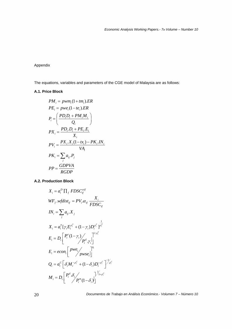
Appendix The equations, variables and parameters of the CGE model of Malaysia are as follows: A.1. Price Block

(1 ).i i iPM pwm tm ER= +

(1 ).i i iPE pwe te ER= −

i i i ii

i

PD D PM MPQ

⎛ ⎞+= ⎜ ⎟⎝ ⎠

. .i i i ii

i

PD D PE EPXX+

=

. (1 ) .i i i i ii

i

PX X tx PK INPVVA− −

=

.i ij jj

PK a P=∑

GDPVAPPRGDP

=

A.2. Production Block

D ifi i f ifX a FDSCα= ∏

. . if if i if

if

XWF wfdist PVFDSC

α=

.i ij jj

IN a X=∑

1

[ (1 ) ]T T Ti i iT

i i i i i iX a E Dρ ρ ργ γ= + − 1/

(1 ).

Tie

i idi i

i i

PE D P

ργ

γ⎡ ⎤−= ⎢ ⎥⎣ ⎦

i

ii i

i

pweE econ pwseη

⎡ ⎤= ⎢ ⎥⎣ ⎦

1

(1 )C C Ci i iC

i i i i i iQ a M Dρ ρ ρδ δ−

− −⎡ ⎤= + −⎣ ⎦

11.

(1 )

Ci

di i

mi ii i

PM D Pρδ

δ+⎡ ⎤= ⎢ ⎥−⎣ ⎦



21

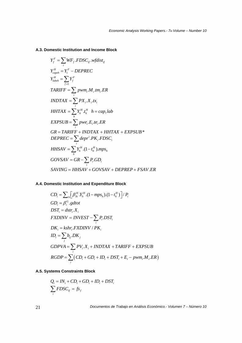
A.3. Domestic Institution and Income Block

. .Ff f if if

iY WF FDSC wfdist=∑

1H F

capehY Y DEPREC= −

1

H Flabeh f

fY Y

≠

= ∑

. . .i i ii

TARIFF pwm M tm ER=∑

. .i i ii

INDTAX PX X tx=∑

. ,H Hh h

hHHTAX Y t h cap lab= =∑

. . .i i ii

EXPSUB pwe E te ER=∑

*GR TARIFF INDTAX HHTAX EXPSUB= + + + . .i

i ii

DEPREC depr PK FDSC=∑

.(1 ).H Hh h h

hHHSAV Y t mps= −∑

.i ii

GOVSAV GR P GD= −∑

.SAVING HHSAV GOVSAV DEPREP FSAV ER= + + + A.4. Domestic Institution and Expenditure Block

. .(1 ).(1 ) /H H Hi ih h h h ih

CD Y mps t Pβ⎡ ⎤= − −⎣ ⎦∑

.Gi iGD gdtotβ=

.i i iDST dstr X=

.i ii

FXDINV INVEST P DST= −∑

. /i i iDK kshr FXDINV PK=

.i ij jj

ID b DK=∑

.i ii

GDPVA PV X INDTAX TARIFF EXPSUB= + + +∑

( ). .i i i i i i ii

RGDP CD GD ID DST E pwm M ER= + + + + −∑

A.5. Systems Constraints Block

i i i i i iQ IN CD GD ID DST= + + + +

if fi

FDSC fs=∑



22

. .i i i ipwm M pwe E FSAV= +

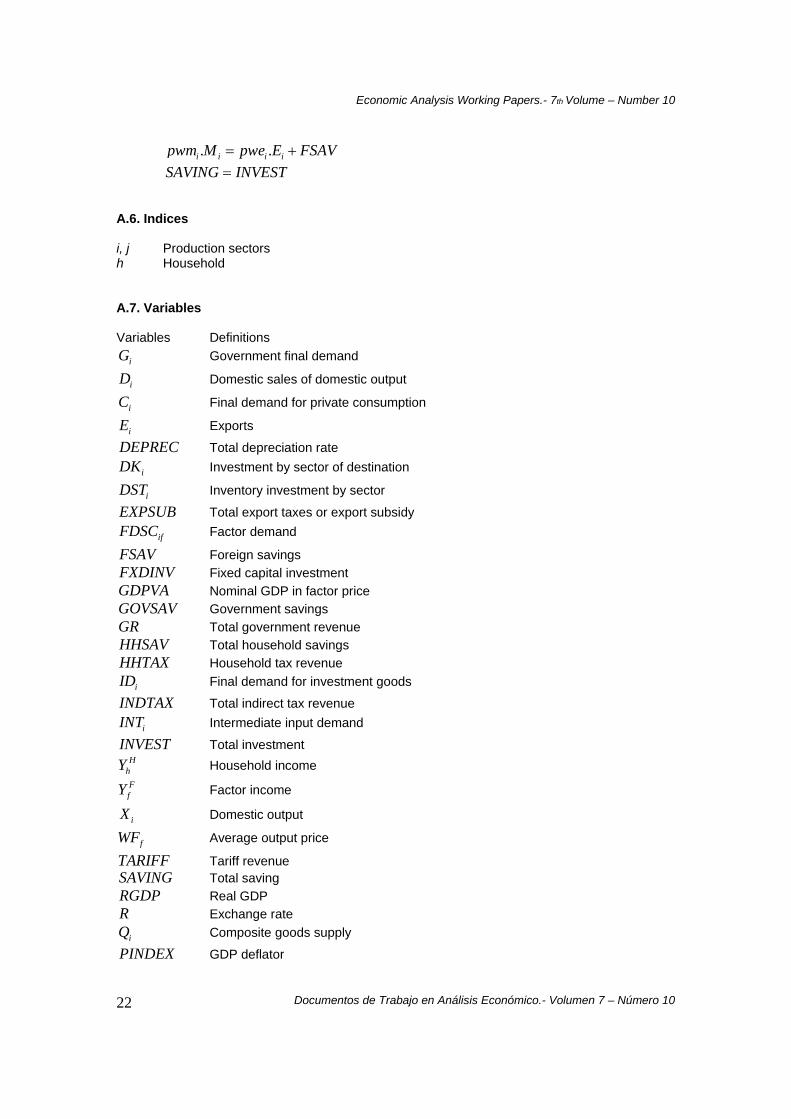
SAVING INVEST= A.6. Indices i, j Production sectors h Household A.7. Variables Variables Definitions

iG Government final demand

iD Domestic sales of domestic output

iC Final demand for private consumption

iE Exports

DEPREC Total depreciation rate

iDK Investment by sector of destination

iDST Inventory investment by sector

EXPSUB Total export taxes or export subsidy

ifFDSC Factor demand

FSAV Foreign savings FXDINV Fixed capital investment GDPVA Nominal GDP in factor price GOVSAV Government savings GR Total government revenue HHSAV Total household savings HHTAX Household tax revenue

iID Final demand for investment goods

INDTAX Total indirect tax revenue

iINT Intermediate input demand

INVEST Total investment H

hY Household income FfY Factor income

iX Domestic output

fWF Average output price

TARIFF Tariff revenue SAVING Total saving RGDP Real GDP R Exchange rate

iQ Composite goods supply

PINDEX GDP deflator



23

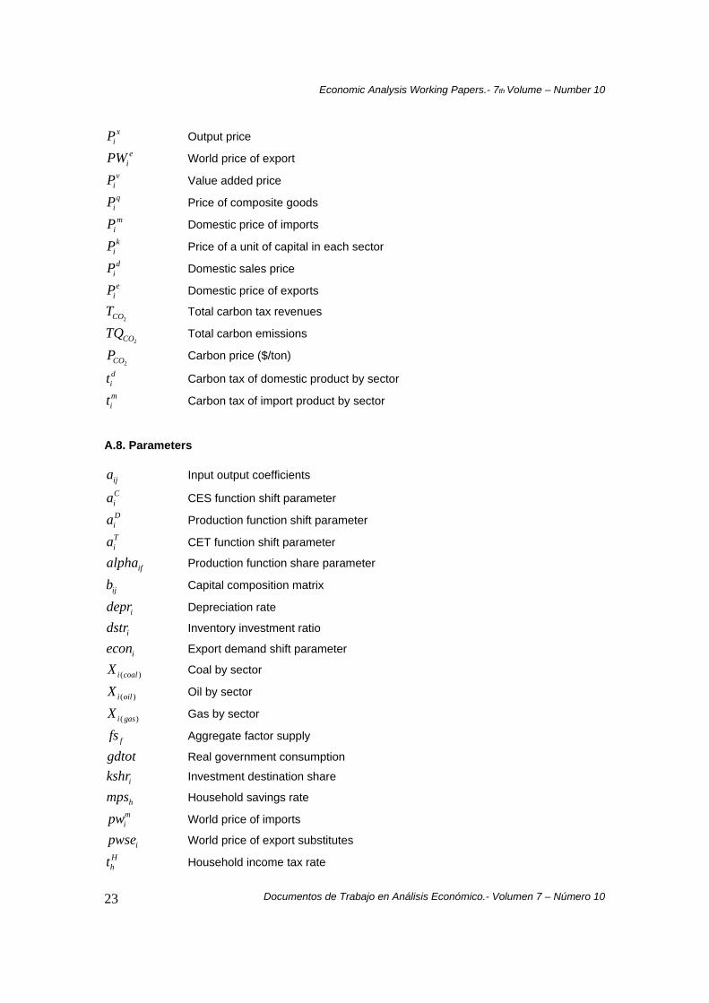
xiP Output price

eiPW World price of export

viP Value added price q

iP Price of composite goods m

iP Domestic price of imports k

iP Price of a unit of capital in each sector d

iP Domestic sales price e

iP Domestic price of exports

2COT Total carbon tax revenues

2COTQ Total carbon emissions

2COP Carbon price ($/ton) dit Carbon tax of domestic product by sector mit Carbon tax of import product by sector

A.8. Parameters

ija Input output coefficients Cia CES function shift parameter Dia Production function shift parameter Tia CET function shift parameter

ifalpha Production function share parameter

ijb Capital composition matrix

idepr Depreciation rate

idstr Inventory investment ratio

iecon Export demand shift parameter

( )i coalX Coal by sector

( )i oilX Oil by sector

( )i gasX Gas by sector

ffs Aggregate factor supply

gdtot Real government consumption

ikshr Investment destination share

hmps Household savings rate mipw World price of imports

ipwse World price of export substitutes Hht Household income tax rate



24

eit Export tax/subsidy rate mit Tariff rate on imports xit Indirect tax rate

ifwfdist Factor market distortion parameter

ijα Production function exponent Giβ Government expenditure share Hihβ Household expenditure shares

iδ CES function share parameter

iη Export demand price elasticity

iγ CET function share parameter Ciρ CES function exponent Tiρ CET function exponent

IMPACTS OF EXTERNAL PRICE SHOCKS ON MALAYSIAN … · Economic Analysis Working Papers.- 7th Volume...

Documents

Transcript of IMPACTS OF EXTERNAL PRICE SHOCKS ON MALAYSIAN … · Economic Analysis Working Papers.- 7th Volume...