IMPACT OF TSUNAMIS ON NEAR SHORE WIND … ABSTRACT . Impact of Tsunamis on Near Shore Wind Power...
95
IMPACT OF TSUNAMIS ON NEAR SHORE WIND POWER UNITS A Thesis by ASHWIN LOHITHAKSHAN PARAMBATH Submitted to the Office of Graduate Studies of Texas A&M University in partial fulfillment of the requirements for the degree of MASTER OF SCIENCE December 2010 Major Subject: Ocean Engineering
Transcript of IMPACT OF TSUNAMIS ON NEAR SHORE WIND … ABSTRACT . Impact of Tsunamis on Near Shore Wind Power...

IMPACT OF TSUNAMIS ON NEAR SHORE WIND POWER UNITS
A Thesis
by
ASHWIN LOHITHAKSHAN PARAMBATH
Submitted to the Office of Graduate Studies of
Texas A&M University
in partial fulfillment of the requirements for the degree of
MASTER OF SCIENCE
December 2010
Major Subject: Ocean Engineering

Impact of Tsunamis on Near Shore Wind Power Units
Copyright 2010 Ashwin Lohithakshan Parambath

IMPACT OF TSUNAMIS ON NEAR SHORE WIND POWER UNITS
A Thesis
by
ASHWIN LOHITHAKSHAN PARAMBATH
Submitted to the Office of Graduate Studies of
Texas A&M University
in partial fulfillment of the requirements for the degree of
MASTER OF SCIENCE
Approved by:
Co-Chairs of Committee, Juan Horrillo
Patrick Lynett
Committee Members, Vijay Panchang
Prabir Daripa
Head of Department, John Niedzwecki
December 2010
Major Subject: Ocean Engineering
iii
ABSTRACT
Impact of Tsunamis on Near Shore Wind Power Units.
(December 2010)
Ashwin Lohithakshan Parambath, B. Tech (Civil), National Institute of
Technology Calicut
Co-Chairs of Advisory Committee: Dr. Juan Horrillo Dr. Patrick Lynett
With the number of wind power units (WPUs) on the rise worldwide, it is
inevitable that some of these would be exposed to natural disasters like tsunamis and it
will become a necessity to consider their effects in the design process of WPUs. This
study initially attempts to quantify the forces acting on an existing WPU due to a
tsunami bore impact. Surge and bore heights of 2m, 5m and 10m are used to compute
the forces using the commercially available full 3D Navier Stokes equation solver
FLOW3D. The applicability of FLOW3D to solve these types of problems is examined
by comparing results obtained from the numerical simulations to those determined by
small scale laboratory experiments. The simulated tsunami forces on the WPU are input
into a simplified numerical structural model of the WPU to determine its dynamic
response. The tsunami force is also used to obtain base excitation which when applied on
the WPU would be equivalent dynamically to the tsunami forces acting on it. This base
excitation is useful to obtain the response of the WPU experimentally, the setup for
which is available at University of California, San Diego's (UCSD) Large High
iv
Performance Outdoor Shake Table (LHPOST). The facility allows full scale
experimental setup capable of subjecting a 65kW Nordtank wind turbine to random base
excitations. A stress analysis of turbine tower cross section is performed in order to
assess the structural integrity of the WPU. It has been determined that the WPU is unsafe
for bore/surge heights above 5 m. It has also been postulated that the structural responses
could be considerable in case of the taller multi megawatt wind power units of present
day.
v
DEDICATION
This thesis is dedicated to my grandpa. Alzheimer’s disease made you forget your last
meal and even your own home for the last 30 years, but you never forgot the fact that
“Achu is studying in America”. It is dedicated to a sweet small girl, Rammu. You
laughed a lot the day I told you, “Thoda pane ke liye, thoda khona bhi padtha hain (To
gain a little, you have to lose a little).” Never did I know that I had to lose you to learn so
much about life. It is also dedicated to my parents and sissy, for their love has been
unconditional.
vi
ACKNOWLEDGEMENTS
I would like to thank my committee chairs, Dr. Juan Horrillo and Dr. Patrick Lynett, for
guiding me through this challenging thesis. patience and industry in helping me tackle
my problems is greatly appreciated. I would also like to thank him for taking me to
Alaska, the most beautiful place on earth, where the idea for this thesis was conceived.
I would also like to thank my committee members Dr Prabir Daripa and Dr.
Patrick Lynett for their valuable feedback and guidance. I would also like to thank Dr.
Vijay Panchang for granting me an opportunity to work under him. I would also like to
thank him for all those wonderful parties that his family has hosted for us and also for
telling the world that his students (Abhishek and me) had caught a shark!
I would like to thank my family for supporting my decisions in life and stepping
in to help whenever things got out of my control. If I ever were to fall on my way, you
would unconditionally help me get back on my feet, is all the confidence that I ever
need. I would also like to thank my friends and colleagues for all the support that they
have rendered in the successful completion of this thesis. My special thanks go out to
Viji, she made me laugh on those days when it hurt real badly, and she

vii
TABLE OF CONTENTS
Page
ABSTRACT ..................................................................................................................... iii
DEDICATION ................................................................................................................. v
ACKNOWLEDGEMENTS ............................................................................................. vi
TABLE OF CONTENTS ................................................................................................. vii
LIST OF FIGURES ......................................................................................................... ix
LIST OF TABLES ........................................................................................................... xii
1. INTRODUCTION AND LITERATURE REVIEW ..................................................... 1
2. THEORETICAL CONSIDERATIONS ........................................................................ 7
2.1 Hydrodynamic Model ................................................................................... 7 2.1.1 Governing Equations and Discretization ...................................... 8 2.1.2 Temporal Discretization ............................................................... 9 2.1.3 Spatial Discretization ................................................................. 11
2.1.3.1 Continuity Equation ................................................. 11
2.1.3.2 2D Momentum Equation Discretization .................. 13 2.1.4 Free Surface Tracking, Volume of Fluid (VOF) ........................ 14 2.1.5 Boundary Conditions .................................................................. 15
2.1.5.1 Wall Boundary Condition ......................................... 16 2.1.5.2 Outflow Boundary Condition ................................... 16
2.1.5.3 Velocity Boundary Condition .................................. 17
2.1.6 Stability Criterion ....................................................................... 17 2.1.7 FLOW-3D .................................................................................. 18
2.2 Structural Stress Analysis Model ................................................................ 19
2.3 Structural Dynamics Model ........................................................................ 19
3. VALIDATION ............................................................................................................ 24
3.1 Hydrodynamic Model versus Experimental Setup ..................................... 24 3.2 Comparison of Results ................................................................................ 26
3.3 Conclusions ................................................................................................. 28
4. QUANTIFICATION OF FORCES ON WPU ............................................................ 29
viii
Page
4.1 Establishing a Computational Domain ....................................................... 29 4.2 Physics Constrains ...................................................................................... 32 4.3 Boundary Conditions .................................................................................. 33 4.4 Numerical Schemes .................................................................................... 34 4.5 Simulation ................................................................................................... 34 4.6 Discussion of Results .................................................................................. 35
5. STRUCTURAL RESPONSE AND INTEGRITY ...................................................... 38
5.1 Description of WPU.................................................................................... 38 5.2 Static Structural Analysis............................................................................ 39
5.2.1 Numerical Modeling .................................................................. 39 5.2.2 Discussion of Results ................................................................. 41
5.3 Dynamic Structural Analysis ...................................................................... 49 5.4 Determination of Base Excitation ............................................................... 53 5.5 Base Excitation of WPU ............................................................................. 54 5.6 Results and Discussions .............................................................................. 55
6. SUMMARY AND FUTURE RESEARCH ................................................................ 58
6.1 Summary ..................................................................................................... 58 6.2 Future Recommendations ........................................................................... 59
6.2.1 Response of MDOF Turbine Model ........................................... 59 6.2.2 Effect on Components ................................................................ 60 6.2.3 Experimental Validation ............................................................ 61
6.3 Conclusions ................................................................................................. 61
REFERENCES .................................................................................................................. 63
APPENDIX A DESCRIPTION OF THE PARTS OF A WIND POWER UNIT .......... 66
APPENDIX B DETERMINATION OF BASE EXCITATION ..................................... 68
APPENDIX C TEMPORAL PROGRESSION OF 5 M SURGE ................................... 70
APPENDIX D RESPONSE OF THE WPU TO TSUNAMI LOADINGS .................... 73
VITA ................................................................................................................................. 82

ix
LIST OF FIGURES
Page
Figure 1 Near shore WPU susceptible to tsunami hazard, located at Hull,
Massachusetts in Boston Harbor........................................................................ 2
Figure 2 Two dimensional grid cell for the discretization of the continuity equation .... 12
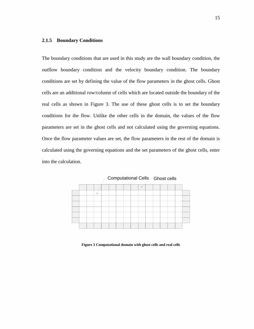
Figure 3 Computational domain with ghost cells and real cells ..................................... 15
Figure 4 Typical modal load function ............................................................................. 23
Figure 5 Experimental setup used to validate hydrodynamic model (Arnason, Petroff
and Yeh [2]) ..................................................................................................... 25
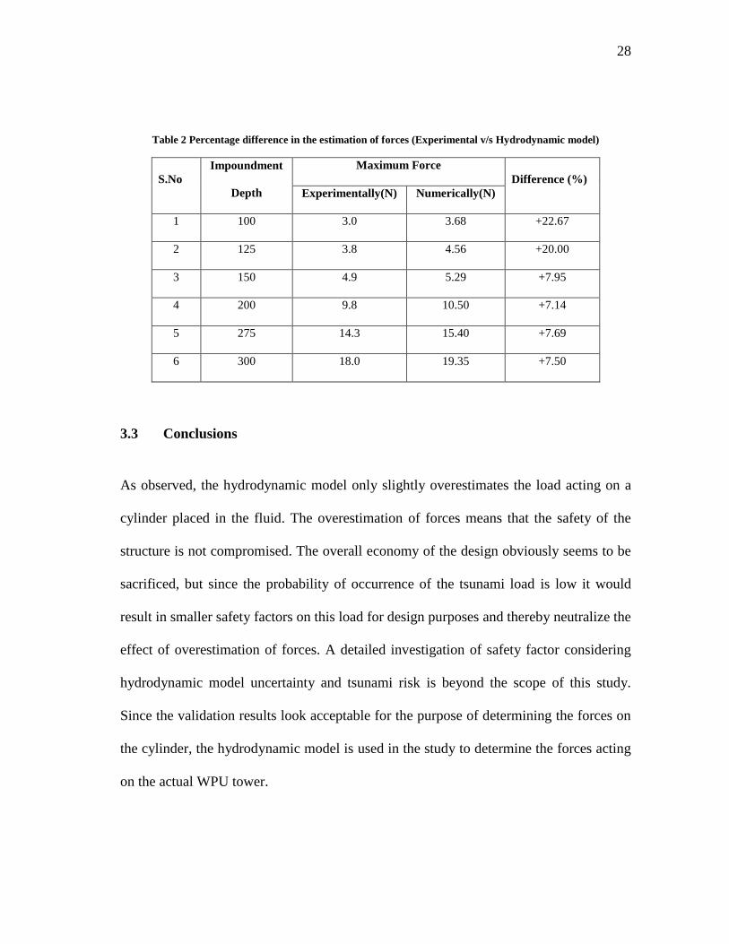
Figure 6 Forces acting on cylinder from Arnason et al [3] experiment .......................... 27
Figure 7 Forces acting on cylinder calculated by FLOW3D .......................................... 27
Figure 8 Computational domain and orientation of the coordinate system .................... 31
Figure 9 Mesh resolutions near the cylinder ................................................................... 32
Figure 10 Forces on cylinder due to 2 m bore/surge ........................................................ 36
Figure 11 Forces on cylinder due to 5 m surge/bore ........................................................ 37
Figure 12 Forces on cylinder due to 10 m surge/bore ...................................................... 37
Figure 13 Determination of forces at the structural node ................................................. 40
Figure 14 Stress distribution along WPU due to 2 m bore (unit: Pa) ............................... 43
Figure 15 Stress distribution along WPU due 2 m surge (unit: Pa) ................................. 44
Figure 16 Stress distribution along WPU due to 5m bore (unit: Pa) ................................ 45
Figure 17 Stress distribution along WPU due to 5 m surge (unit: Pa) ............................. 46
Figure 18 Stress distribution along WPU due to 10 m bore (unit: Pa) ............................. 47
Figure 19 Stress distribution along WPU due to 10 m surge (unit: Pa) ........................... 48
x
Page
Figure 20 Force transformation ........................................................................................ 50
Figure 21 Sketch of 65kW Nordtank Wind Turbine, showing observation points for
structural response, Adopted from [20] ........................................................... 52
Figure 22 Representative sketch A) dynamic system with time history forcing; B)
dynamic system with base excitation forcing. ................................................. 53
Figure 23 Spectral energy of accelerations at J1 .............................................................. 56
Figure 24 Spectral Energy of accelerations at J2 ............................................................. 56
Figure 25 Spectral energy of accelerations at J3 .............................................................. 57
Figure 26 Parts of a WPU (source: [25]) .......................................................................... 66
Figure 27 Simplified 1D dynamic system ........................................................................ 68
Figure 28 Pressure contour 5 m surge (time = 0.3 secs) .................................................. 70
Figure 29 Pressure contour 5 m surge (time = 1.5 secs) .................................................. 71
Figure 30 Pressure contour surge 5 m (time = 2.5 secs) .................................................. 71
Figure 31 Pressure contour surge 5 m (time = 3.1 secs) .................................................. 72
Figure 32 Responses at Joint J1 for 2 m bore .................................................................. 73
Figure 33 Responses at Joint J2 for 2 m bore .................................................................. 73
Figure 34 Responses at Joint J3 for 2 m bore .................................................................. 74
Figure 35 Responses at Joint J1 for 2 m surge ................................................................. 74
Figure 36 Responses at Joint J2 for 2 m surge ................................................................. 75
Figure 37 Responses at Joint J3 for 2 m surge ................................................................. 75
Figure 38 Responses at Joint J1 for 5 m bore .................................................................. 76
Figure 39 Responses at Joint J2 for 5 m bore .................................................................. 76
xi
Page
Figure 40 Responses at Joint J3 for 5 m bore .................................................................. 77
Figure 41 Responses at Joint J1 for 5 m surge ................................................................. 77
Figure 42 Responses at Joint J2 for 5 m surge ................................................................. 78
Figure 43 Responses at Joint J3 for 5 m surge ................................................................. 78
Figure 44 Responses at Joint J1 for 10 m bore ................................................................ 79
Figure 45 Responses at Joint J2 for 10 m bore ................................................................ 79
Figure 46 Responses at Joint J3 for 10 m bore ................................................................ 80
Figure 47 Responses at Joint J1 for 10 m surge ............................................................... 80
Figure 48 Responses at Joint J2 for 10 m surge ............................................................... 81
Figure 49 Responses at Joint J2 for 10 m surge ............................................................... 81

xii
LIST OF TABLES
Page
Table 1 Computational domain specifications for different impoundment depths .......... 26
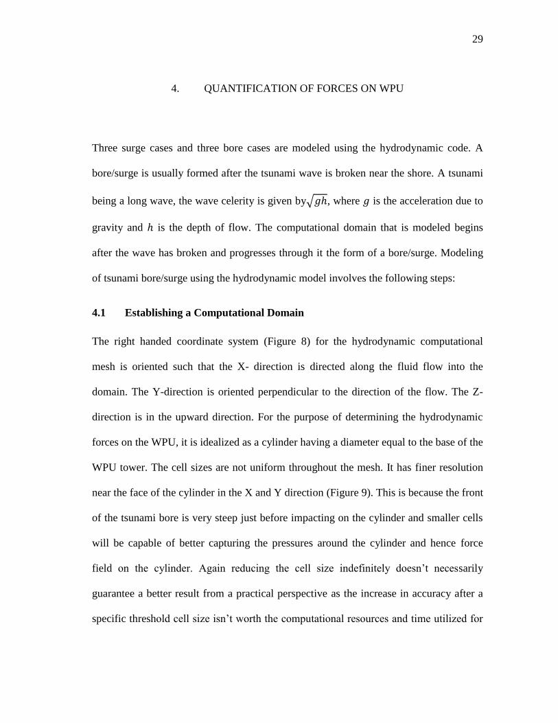
Table 2 Percentage difference in the estimation of forces (Experimental v/s
Hydrodynamic model) ........................................................................................ 28
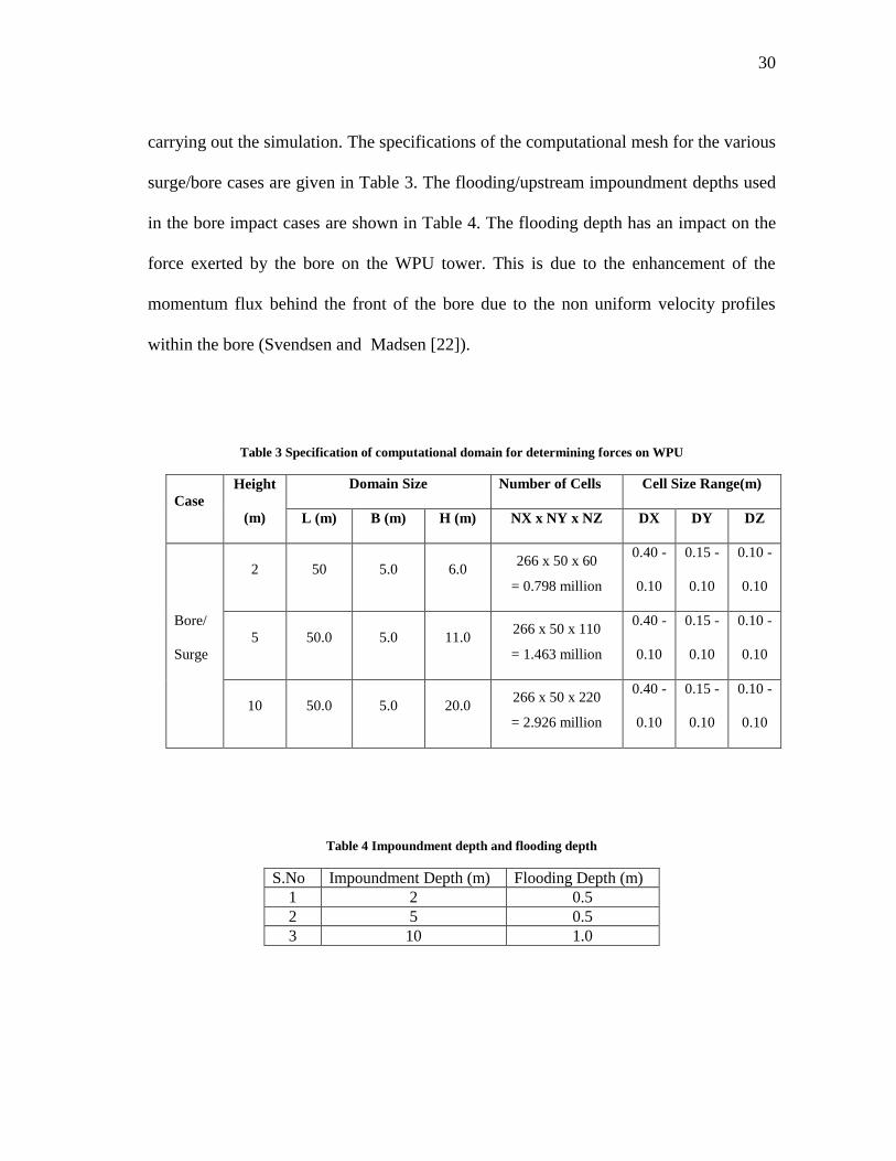
Table 3 Specification of computational domain for determining forces on WPU ........... 30
Table 4 Impoundment depth and flooding depth ............................................................. 30
Table 5 Computation times for various surge/bore cases................................................. 35
Table 6 Properties of 65kW Nordtank Turbine. Source [20] ........................................... 41
Table 7 Modal frequencies and cumulative mass participation ....................................... 51
This thesis follows the style of Journal of Earthquake Engineering and Structural
Dynamics.
1
1. INTRODUCTION AND LITERATURE REVIEW
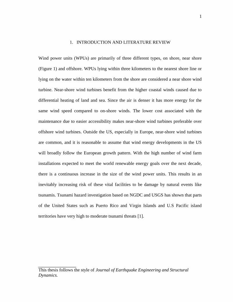
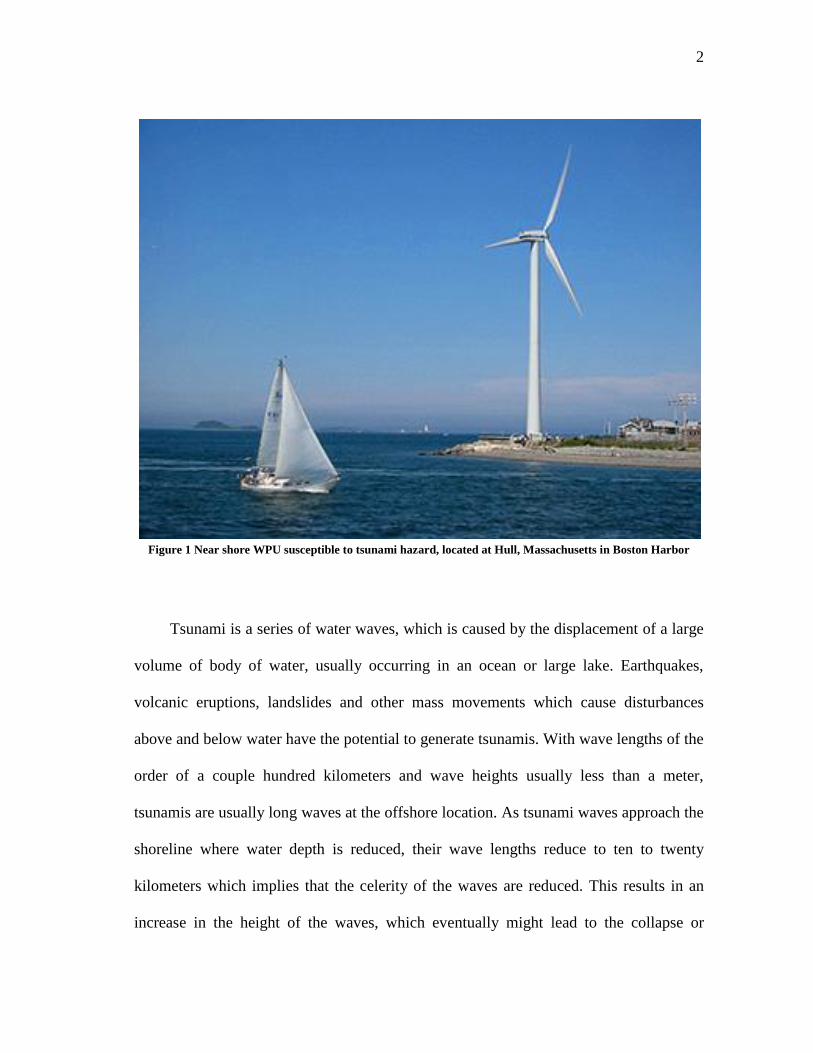
Wind power units (WPUs) are primarily of three different types, on shore, near shore
(Figure 1) and offshore. WPUs lying within three kilometers to the nearest shore line or
lying on the water within ten kilometers from the shore are considered a near shore wind
turbine. Near-shore wind turbines benefit from the higher coastal winds caused due to
differential heating of land and sea. Since the air is denser it has more energy for the
same wind speed compared to on-shore winds. The lower cost associated with the
maintenance due to easier accessibility makes near-shore wind turbines preferable over
offshore wind turbines. Outside the US, especially in Europe, near-shore wind turbines
are common, and it is reasonable to assume that wind energy developments in the US
will broadly follow the European growth pattern. With the high number of wind farm
installations expected to meet the world renewable energy goals over the next decade,
there is a continuous increase in the size of the wind power units. This results in an
inevitably increasing risk of these vital facilities to be damage by natural events like
tsunamis. Tsunami hazard investigation based on NGDC and USGS has shown that parts
of the United States such as Puerto Rico and Virgin Islands and U.S Pacific island
territories have very high to moderate tsunami threats [1].
2
Figure 1 Near shore WPU susceptible to tsunami hazard, located at Hull, Massachusetts in Boston Harbor
Tsunami is a series of water waves, which is caused by the displacement of a large
volume of body of water, usually occurring in an ocean or large lake. Earthquakes,
volcanic eruptions, landslides and other mass movements which cause disturbances
above and below water have the potential to generate tsunamis. With wave lengths of the
order of a couple hundred kilometers and wave heights usually less than a meter,
tsunamis are usually long waves at the offshore location. As tsunami waves approach the
shoreline where water depth is reduced, their wave lengths reduce to ten to twenty
kilometers which implies that the celerity of the waves are reduced. This results in an
increase in the height of the waves, which eventually might lead to the collapse or
3
breaking of the wave. Once broken these waves propagate on to the shore. Among the
various ways in which a tsunami can propagate onshore, the common one is that of a
rapidly advancing hydraulic bore which is formed by the breaking of the tsunami wave
at the offshore reef or at the shoreline. This type of wave front is one of the most
destructive forms of onshore propagation of tsunamis (Arnason, Petroff and Yeh, [2])
and this study proposes to use this type of tsunami propagation onto the WPU structure.
The bore consists of a turbulent front, which being steep exerts a large force on any
objects in its path. In general, tsunami bores might propagate over dry land, in which
case they are referred to as a surge or over an existing inundation or flowing water in
which case they are called wet bores.
In the past, considerable research has gone into predicting the runup of tsunami
waves, as these help to estimate the inundation caused in the coastal areas due to a
tsunami. Very few studies have however tried to address the problem of estimating the
forces exerted by a tsunami bore on coastal structures. With onshore propagation speeds
of the order of nearly 10 m/s and surge heights up to 30 m in extreme cases (Arnason
[3]), the force imparted to the coastal structures are considerable. Most of these studies
however tried to quantify the forces on vertical walls [4] and other structures which are
common among coastal regions. As WPUs have been in existence only recently, there
are not any known studies which evaluate the temporal variation of the tsunami force
acting on a WPU.
4
One of the techniques that is used to solve such problems is to experimentally
quantify the forces. This, however, poses new challenges, such as the generation of a
tsunami bore in a laboratory. Chanson [5] has shown that there exist similarities between
a tsunami front and a dam break problem and this fact has been used to tackle the
problem of tsunami generation in a laboratory. Dam break problems have been
extensively studied in the past and often the tsunami bore is generated by opening
experimentally/numerically a gate with water impounded on one side. Chanson [5] had
developed a simplified numerical solution to a dam break problem in order to determine
its height and velocity. He argued that a dam break resulted in a hydraulic jump which is
very similar to a tsunami bore. Then he compared the results that were obtained from the
solution of dam break to some of the data sets recorded from tsunami surges on dry
coastal plains that had previously occurred. He observed that the solution to the dam
break problem was sufficiently capable of predicting the tsunami runup onto the coast.
Arnason [3] used the same fact to experimentally create a tsunami bore in a wave tank
and allowed it to impinge on a circular/square tubular kept in the wave tank. The same
experiment was repeated to determine the forces acting on the cylinder for various bore
heights. However, these results are for small scaled models. The result obtained cannot
be scaled up to estimate the variation of the forces with time for the actual WPU tower,
as determination of a scaling factor would pose a challenging task. Hence in order to
simplify the problem, numerical models are needed to be developed to quantify the
forces imparted by a tsunami impact. These numerical models however could be
validated using the results obtained from the small scaled experiments.
5
One of the first models to quantify the forces due to a tsunami on a cylindrical
structure was developed by Davletshin and Lappo [6]. They studied the tsunami using
three different cases. In the first case, the tsunami is treated as a large unbroken wave, in
the second, it is treated as a solitary wave, and in the third, the tsunami is treated as a
surge, resulting from the breaking of a large wave. They used the shallow water
equations to solve the pressure field in the vicinity of a cylinder placed in water. This,
however, pose a problem as these shallow water models are incapable of capturing the
vertical variation of the velocity/acceleration in case of a tsunami runup and the effects
could considerably vary the force acting on objects placed in the flow [7]. The vertical
variation of the velocity/acceleration can be captured using a full 3D Navier Stokes
Equation (NSE) solver.
The use of solitary waves in the study of tsunami runup onto a coast is quiet
common (Synolakis [8], Mo, et al. [9]). The solitary wave, upon reaching shallow
depths, breaks and the surge/bore which is formed as a result is allowed to propagate on
the coast. But this study proposes to use the dam break method to mimic the last stage of
a broken solitary wave to numerically determine forces on a WPU as it is believed that it
is able to capture the steep front of an actual tsunami bore/surge. Also the differences in
forces due to a bore or surge as shown by Nistor [10] and Yeh [11] are only evident
when the dam break method of tsunami generation is used. As shown by the
investigators [12] a NSE solver with the free surface tracked using the Volume of Fluids
method is capable of capturing the forces due to a dam break. Once the forces have been
6
determined accounting for these factors; the next task would be to study the impact of
these forces on the structural behavior of the WPU.
WPU is a complex structure as it has multiple degrees of freedom (DOF’s). Some
of the DOF’s are rotational DOF’s, and the deflections violate the small deflection
theory. Moreover, a WPU has a gyroscopic moment caused due to the rotation of its
blades. These are capable of generating considerable forces in a WPU tower, when
coupled with the dynamic response of the WPU tower under the impact of tsunami load.
Though some studies have looked into the effect of tsunami loading on different types of
structures [13], hitherto no study has looked into the effect of a tsunami loading on a
WPU. Hence there is a necessity to determine the dynamic response of the WPU tower
to this loading. There is also the necessity of looking into the stresses induced in the
structure due to tsunami loading, in order to assess the integrity of the structure under the
effect of this loading.
The study also proposes to carry out an experimental validation of the results
obtained from dynamic analyses of the structure as a future initiative. The University of
California, San Diego (UCSD) has the experimental setup capable of carrying out these
validations, which consists of a Large High Performance Outdoor Shake Table
(LHPOST), capable of shaking a 65 kW Nordtank Wind Turbine. This setup can also be
used to study the effect of the coupling of the dynamics of various components of the
WPU with that of the tower.
7
2. THEORETICAL CONSIDERATIONS
2.1 Hydrodynamic Model
Computational Fluid Dynamics (CFD) is one of the branches of the fluid dynamics that
uses numerical methods and algorithms to solve and analyze problems that involve fluid
flows. The fundamental basis of almost all CFD problems is the Navier Stokes equation
along with the mass conservation equation. These are the governing equations that can
describe almost any of the physical properties of a flow. However these equations are
very difficult to solve theoretically and require approximations of the same to obtain
solutions to problems for practical applications. Various techniques such as finite
difference, finite volume, finite element and spectral methods are used to solve these
equations.
In this study, a full 3D Navier Stokes equation (NSE) solver is used to model the
flow in order to capture the forces exerted by the fluid on the WPU. Two dimensional,
hydrostatic models which are usually used to study the progression of tsunami waves
take into account only the depth integrated horizontal velocities and the water surface
elevations are calculated by the mass conservation equation. These models work well for
the determination of tsunami propagation through the ocean. But in case of tsunami
generation and runup, the vertical variation of the velocity/acceleration is significant. A
Navier-Stokes approach is more suitable for these problems as: 1) it includes the vertical
variation of the velocity/acceleration and 2) it helps to better estimate the forces applied
by the flow on any structure in the path of the flow. This is because the pressure
8
obtained from NSE solver is non hydrostatic unlike the depth-integrated long wave
models where it is hydrostatic.
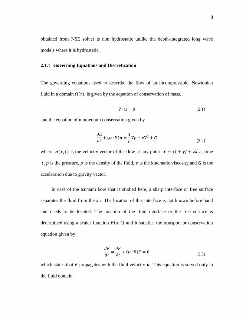
2.1.1 Governing Equations and Discretization
The governing equations used to describe the flow of an incompressible, Newtonian
fluid in a domain , is given by the equation of conservation of mass,
(2.1)
and the equation of momentum conservation given by
(2.2)
where, is the velocity vector of the flow at any point at time
, is the pressure, is the density of the fluid, is the kinematic viscosity and is the
acceleration due to gravity vector.
In case of the tsunami bore that is studied here, a sharp interface or free surface
separates the fluid from the air. The location of this interface is not known before hand
and needs to be located. The location of the fluid interface or the free surface is
determined using a scalar function and it satisfies the transport or conservation
equation given by
(2.3)
which states that propagates with the fluid velocity . This equation is solved only in
the fluid domain.

9
For solving these equations, the entire domain (both fluid and air) is first
discretized into cells which are rectangles (2D) or cubes (3D). Each cell is uniquely
identified using a vector where and
with equal to the number of cells in the and direction
respectively. These cells can be of non uniform sizes and this facilitates the use of a
higher resolution where the flow parameters vary drastically and lower resolution
elsewhere. Each cell has a size given by and in the and direction
respectively. The velocity associated with a cell is located at the right, back
and the top face of the cell. The parameters such as pressure , volume of fluid
fraction , are located at the center of the cell (described in 2.1.4).
For any flow in a domain, the parameters such as and are known at time
. The governing equations can then be solved by discretizing them spatially and
temporally in order to obtain the flow parameters in the domain at any required time.
2.1.2 Temporal Discretization
The continuity equation (2.1) and the momentum equation (2.2) are discretized in time
by using an explicit forward Euler method, which reads
(2.4)
and
(2.5)
10
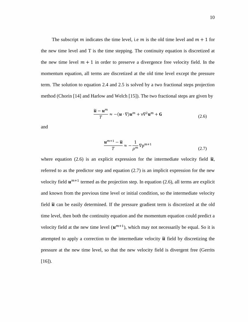
The subscript indicates the time level, i.e is the old time level and for
the new time level and T is the time stepping. The continuity equation is discretized at
the new time level in order to preserve a divergence free velocity field. In the
momentum equation, all terms are discretized at the old time level except the pressure
term. The solution to equation 2.4 and 2.5 is solved by a two fractional steps projection
method (Chorin [14] and Harlow and Welch [15]). The two fractional steps are given by
(2.6)
and
(2.7)
where equation (2.6) is an explicit expression for the intermediate velocity field ,
referred to as the predictor step and equation (2.7) is an implicit expression for the new
velocity field termed as the projection step. In equation (2.6), all terms are explicit
and known from the previous time level or initial condition, so the intermediate velocity
field can be easily determined. If the pressure gradient term is discretized at the old
time level, then both the continuity equation and the momentum equation could predict a
velocity field at the new time level ( ), which may not necessarily be equal. So it is
attempted to apply a correction to the intermediate velocity field by discretizing the
pressure at the new time level, so that the new velocity field is divergent free (Gerrits
[16]).
11
This results in an equation obtained by combining equation (2.7) and the continuity
equation (2.4), which can be solved to obtain the pressure at the new time level given by
(2.8)
which is known as the Pressure Poisson Equation (PPE). The finite difference of this
equation would result in a system of linear equation which can be solved iteratively
using methods such as successive over relaxation (SOR), generalized minimal
residual(GMRES) and incomplete Cholesky conjugate gradient. From here the velocity
field at the new time level ( ) can be determined by substituting this value in
projection step, which becomes
(2.9)
2.1.3 Spatial Discretization
2.1.3.1 Continuity Equation
To ensure global mass conservation, i.e., the total amount of fluid in the entire
computational domain, and local conservation, i.e., the amount of fluid in the
computational cell, the change in the surface level must be consistent with the mass
fluxes. For sake of simplicity consider a two dimensional (2D) computational cell ( )
in the domain. The control volume at cell center, , is bounded by
and as shown in Figure 2. For spatial discretization, first
the continuity equation (2.1) is discretized and results in

12
(2.10)
where is the horizontal velocity at the right face of the cell, is the horizontal
velocity at the left face of the cell, is the vertical velocity at the top face of the cell
and is the vertical velocity at the bottom face of the cell. is the area fraction
open to the flow at the right face of the cell, is the area open to the flow at the
left face of the cell, is the area open to the flow at the top face of the cell and
is the area open to the flow at the bottom face of the cell.
Figure 2 Two dimensional grid cell for the discretization of the continuity equation
13
Area fraction is the quantity that decides how much of the cell is open to a flow.
This is used, because partly blocked cells, such as the ones near an obstruction or at the
bottom, if treated as a completely blocked cell, would result in a discrete step, which is
not desirable especially when modeling complex geometries. Hence an area fraction is
determined for every cell, which is the fraction of the area, at a particular face open to
the flow or in other words, it is the fractional aperture of the cell that is open to the flow.
This technique of using area fraction is also known as Fractional Area Volume Obstacle
Representation (FAVOR), Nichols et al [12]; Sicillan and Hirt [17]; Gentry et al [18].
2.1.3.2 2D Momentum Equation Discretization
The momentum equation (2.2) is discretized in the and direction as
(2.11)
and
(2.12)
In these equations, the advection term is in the non conservative form. These terms
are again discretized using a) backward/forward/central difference method (first or
second order approximation), b) third order accurate method. Among these the first

14
order approximation is used in this study and these are obtained from the Taylor’s series
approximations of the velocity.
2.1.4 Free Surface Tracking, Volume of Fluid (VOF)
In the computational domain, it is assumed that the fluid has a constant density given by
and the density of air is zero. The scalar quantity, Volume of Fluid for a cell is
defined as
, where is the density of cell. This implies that a value of ,
implies that the cell is a void cell, indicates a completely filled cell and
, implies that cell is a free surface cell. The volume of fluid is transported through the
fluid using the transport equation as shown below
(2.13)
where accounts cell aperture open to the flow. The temporal discretization of the
above equation is given by
(2.14)
where the bracketed is the amount of volume fraction entering a particular cell at
that face. The spatial discretization of the function is done using the donor acceptor
method as described by Hirt and Nicholes [19], which is a geometric solution for the
volume of fluid fraction entering or leaving a cell, accounting for the effect of free
surface. A detailed explanation of the donor acceptor method is not shown here.
15
2.1.5 Boundary Conditions
The boundary conditions that are used in this study are the wall boundary condition, the
outflow boundary condition and the velocity boundary condition. The boundary
conditions are set by defining the value of the flow parameters in the ghost cells. Ghost
cells are an additional row/column of cells which are located outside the boundary of the
real cells as shown in Figure 3. The use of these ghost cells is to set the boundary
conditions for the flow. Unlike the other cells in the domain, the values of the flow
parameters are set in the ghost cells and not calculated using the governing equations.
Once the flow parameter values are set, the flow parameters in the rest of the domain is
calculated using the governing equations and the set parameters of the ghost cells, enter
into the calculation.
Figure 3 Computational domain with ghost cells and real cells
Ghost cellsComputational Cells

16
The various boundary conditions are set as shown below.
2.1.5.1 Wall Boundary Condition
The wall boundary condition is when any fluid that reaches that cell is not allowed to
pass through that cell. The method for accomplishing this is shown using an example of
a wall boundary at a minimum boundary. The values for the first real cell is set as
(2.15)
2.1.5.2 Outflow Boundary Condition
The outflow boundary condition, also known as the radiation boundary condition is the
one that permits all the fluid that reaches that point to exit the domain without causing
significant effects in the upstream location. Usually the flow is only required to be
modeled in a specific region of the entire fluid domain and these boundary help to cut
off the computational mesh, beyond the region where flow characteristics that are not
required to be calculated. The outflow boundary condition is set by using the
Sommerfeld radiation boundary condition, which is a simple mathematical continuation
having the form of outgoing waves,
17
(2.16)
where is any quantity and is directed out of the boundary and is the local phase
speed of the wave or flow.
2.1.5.3 Velocity Boundary Condition
The velocity boundary condition is set by changing the velocity in the ghost cell to the
value defined by the user. It is possible to vary the velocity defined in the ghost cell with
respect to time. The fluid height is also set here. The values of the ghost cells are set
depending on whether the cell is a filled cell, void cell or a surface cell.
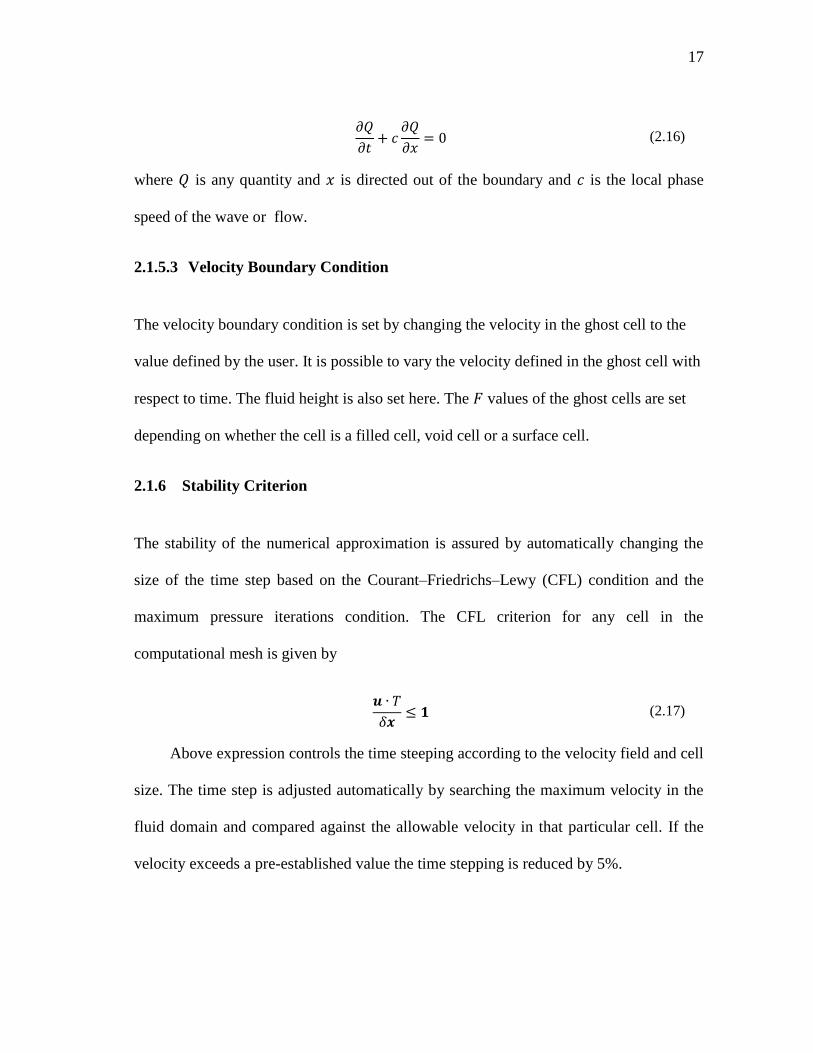
2.1.6 Stability Criterion
The stability of the numerical approximation is assured by automatically changing the
size of the time step based on the Courant–Friedrichs–Lewy (CFL) condition and the
maximum pressure iterations condition. The CFL criterion for any cell in the
computational mesh is given by
(2.17)
Above expression controls the time steeping according to the velocity field and cell
size. The time step is adjusted automatically by searching the maximum velocity in the
fluid domain and compared against the allowable velocity in that particular cell. If the
velocity exceeds a pre-established value the time stepping is reduced by 5%.
18
2.1.7 FLOW-3D
The above mentioned equations are implemented in FLOW-3D, which is a commercial
CFD tool that is capable of solving a wide variety of physical flows. Some of the salient
features of FLOW-3D are:
It uses FAVOR method
Computational grid and geometry are independent
Can handle internal, external and free surface flows
Can handle one, two and three dimensional flows
It can solve transient flows which are inviscid, viscous, laminar and turbulent
Can track fluid interfaces using the VOF method
Advection terms with approximation up to the third order can be solved
Can track sharp fluid interfaces
Has implicit and explicit modeling options
Has the GMRES and SOR implementation for the pressure solver
Can handle many different types of fluid boundaries such as rigid wall,
continuative, periodic, outflow, hydrostatic pressure, etc.
Provisions for changing some of flow properties at runtime using the restart
option
A robust data visualization tool, to visualize the various flow properties such as,
but not restricted to pressure, free surface, velocities, cell fluid fractions and
forces on objects placed in the flow
19
All these features make it a robust tool for carrying out our study and have been
used to solve the hydrodynamic problem.
2.2 Structural Stress Analysis Model
The ANSYS Structural package is used to carry out finite element structural analysis of
the WPU tower structure. The tower which is basically a thin-walled cylinder made up
of three sections, of varying cross sections, is discretized using 4-noded shell elements.
These elements have six degrees of freedom (along three lateral and three rotational
directions) at each of their nodes and they are capable of accounting for variable shell
thickness at each node. However in this study, the shell thickness is considered constant.
The spatial discretization (rectangular) of the model is obtained using the automatic
meshing capability of the structural stress analysis package. The tsunami loads are
applied as nodal loads at each shell elements along its degree of freedom direction. The
thin-walled cylinder is fixed at the bottom using a full fixed boundary condition, i.e. all
the displacements and rotations are restrained at the bottom. The force-stiffness
relationship is used to determine the forces induced in the shell element due to the nodal
loads. The forces are then used to determine the principal stresses induced in the shell
elements. The equivalent stresses or Von Mises stresses induced in the structure are then
determined.
2.3 Structural Dynamics Model
For the purpose of carrying out a dynamic structural analysis, the whole WPU tower is
20
idealized as a dynamic system having 30 discrete masses with each mass having 3
degrees of freedom, two lateral displacements along the and one rotational
displacements along the direction. The coordinate system for carrying out the
dynamic analysis is oriented such that the -axis is along the length of the WPU. The
nacelle (refer Appendix A) and the rotor are idealized as masses at a point at the hub
height of the WPU. The tower is fully fixed to the ground by restraining all
displacements and rotations.
The dynamic analysis of the WPU is carried out using the modal superposition
method. The mass matrix used in the analysis is determined using the consistent mass
matrix method. The damping associated with each modal frequency has been
experimentally obtained [20]. The procedure for obtaining the response of the structure
is as shown below.
According to De Alembert’s principle of inertial forces, any system that has a mass
and is subjected to acceleration would develop an inertial force proportional to its
acceleration and opposing it. If a given N degree of freedom structural system has
stiffness and damping associated with each of its degrees of freedom, the force
equilibrium equation for this system can be written in the following form as a set of N
second order differential equations
(2.18)

21
where is the mass matrix, is damping matrix, is stiffness matrix of the system,
is the time history of the force applied on the system, is the time history of the
response of the system. Further can be expressed in the form
(2.19)
which means that time dependent loading can be represented by a sum of space
vectors , which are not a function of time, and time functions , where
cannot be greater than the number of displacements N. This is another way of saying that
each mass is acted upon by a maximum of only one force along each degree of freedom.
Equation (2.18) is solved by method of separation of variables. A solution to the
equation can be expressed in the form
(2.20)
where is an “N by L” matrix of spatial vectors (not a function of time) which
represents the position of the Nth
mass in the Lth
mode of vibration and is a vector
containing L functions of time, which represent the variation of the Lth
mode with
respect to time. is also known as the mode shape of the structure. The is chosen
such that it satisfies the stiffness and mass orthogonality condition
(2.21)
22
where is the diagonal identity matrix and is a diagonal matrix, which may or may
not be the free vibration frequencies of the system. This equation (2.21) is then
substituted in equations (2.18) and (2.19) to obtain
(2.22)
where and is known as the modal participation factors for time function
. The modal participation factor for the nth
mode is given by . This factor is an
indicator of how much a particular mode participates in the response of the structure.
The damping matrix is usually not a diagonal matrix, but it is assumed to be so that
the equations are uncoupled and this results in a diagonal matrix given by
(2.23)
where is defined as the ratio of the damping in mode to the critical damping of the
mode. Hence the typical uncoupled modal equation, for a linear structural system can be
represented as
(2.24)
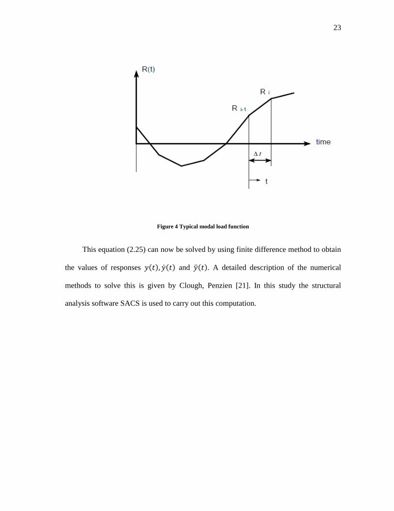
Now if we have an arbitrary modal time history loading, which is piecewise linear and
given by as shown in Figure 4, the equation (2.24) can be expressed as
(2.25)
23
Figure 4 Typical modal load function
This equation (2.25) can now be solved by using finite difference method to obtain
the values of responses and . A detailed description of the numerical
methods to solve this is given by Clough, Penzien [21]. In this study the structural
analysis software SACS is used to carry out this computation.
24
3. VALIDATION
3.1 Hydrodynamic Model versus Experimental Setup
Before FLOW-3D, henceforth referred to as the hydrodynamic model, can be used to
capture the forces exerted by a tsunami bore on a WPU, it has to be verified against the
dam break problem. This is done by validating the hydrodynamic model using the data
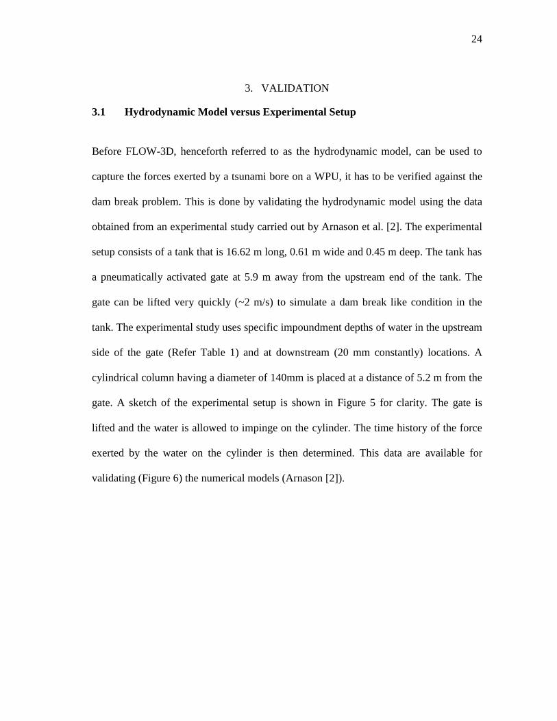
obtained from an experimental study carried out by Arnason et al. [2]. The experimental
setup consists of a tank that is 16.62 m long, 0.61 m wide and 0.45 m deep. The tank has
a pneumatically activated gate at 5.9 m away from the upstream end of the tank. The
gate can be lifted very quickly (~2 m/s) to simulate a dam break like condition in the
tank. The experimental study uses specific impoundment depths of water in the upstream
side of the gate (Refer Table 1) and at downstream (20 mm constantly) locations. A
cylindrical column having a diameter of 140mm is placed at a distance of 5.2 m from the
gate. A sketch of the experimental setup is shown in Figure 5 for clarity. The gate is
lifted and the water is allowed to impinge on the cylinder. The time history of the force
exerted by the water on the cylinder is then determined. This data are available for
validating (Figure 6) the numerical models (Arnason [2]).
25
Figure 5 Experimental setup used to validate hydrodynamic model (Arnason, Petroff and Yeh [2])
The same set of physical experiments is reproduced using the hydrodynamic model
with domain size and resolution indicated in Table 1. The hydrodynamic model has a
provision for defining an initial water depth in the upstream and downstream location at
time t = 0 sec. The water gradient is then allowed to flow under the effect of gravity in a
bore like form towards the cylinder. The hydrodynamic model is capable of capturing
the free surface elevation (sharp discontinuity), velocity vectors, pressure and the forces
acting on the cylinder. The time history of the force acting on the cylinder for various
impoundment depths are shown in Figure 7 (Page 27).
16.8 m
0.45 m
5.9 m 5.2 m
Impoundment Depth
CylinderPneumatic Gate
26
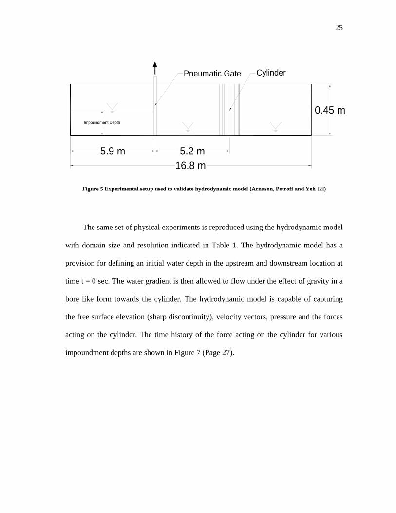
Table 1 Computational domain specifications for different impoundment depths
S.No
Impoundment
Depth(mm)
Domain Size Number of Cells Cell Size
LxBxH (m x m x m) NX x NY x NZ DX (m) DY (m)
DZ
(m)
1 100 16.6 x 0.6 x 0.45 332 x 48 x 9 0.09 - 0.01 0.015-0.01 0.05
2 125 16.6 x 0.6 x 0.45 332 x 48 x 9 0.09 - 0.01 0.015-0.01 0.05
3 150 16.6 x 0.6 x 0.45 332 x 48 x 9 0.09 - 0.01 0.015-0.01 0.05
4 200 16.6 x 0.6 x 0.45 332 x 48 x 9 0.09 - 0.01 0.015-0.01 0.05
5 275 16.6 x 0.6 x 0.45 332 x 48 x 9 0.09 - 0.01 0.015-0.01 0.05
6 300 16.6 x 0.6 x 0.45 332 x 48 x 9 0.09 - 0.01 0.015-0.01 0.05
3.2 Comparison of Results
Figure 6 and Figure 7 show a comparison of the forces on the cylinder obtained
experimentally and using the hydrodynamic model. They show a very good correlation.
It is observed that the forces obtained from the hydrodynamic model follow the same
trend as the experimentally. This agreement indicates that the hydrodynamic model is
capable of capturing most of the characteristics of the flow portrayed in the experimental
study. It is also observed that the forces imparted on the cylinder increases as the
impoundment depth increases, which has also been shown in the studies by Nistor et al
[10] and Yeh [11]. It is determined that the hydrodynamic model over estimates the load
on the cylinder by 8 to 23 percentages (Refer Table 2). It is also determined that the
percentage error in the estimation of the force decreases as the impoundment depth
increases. This is promising as it is usually a challenging task to match the forces exerted
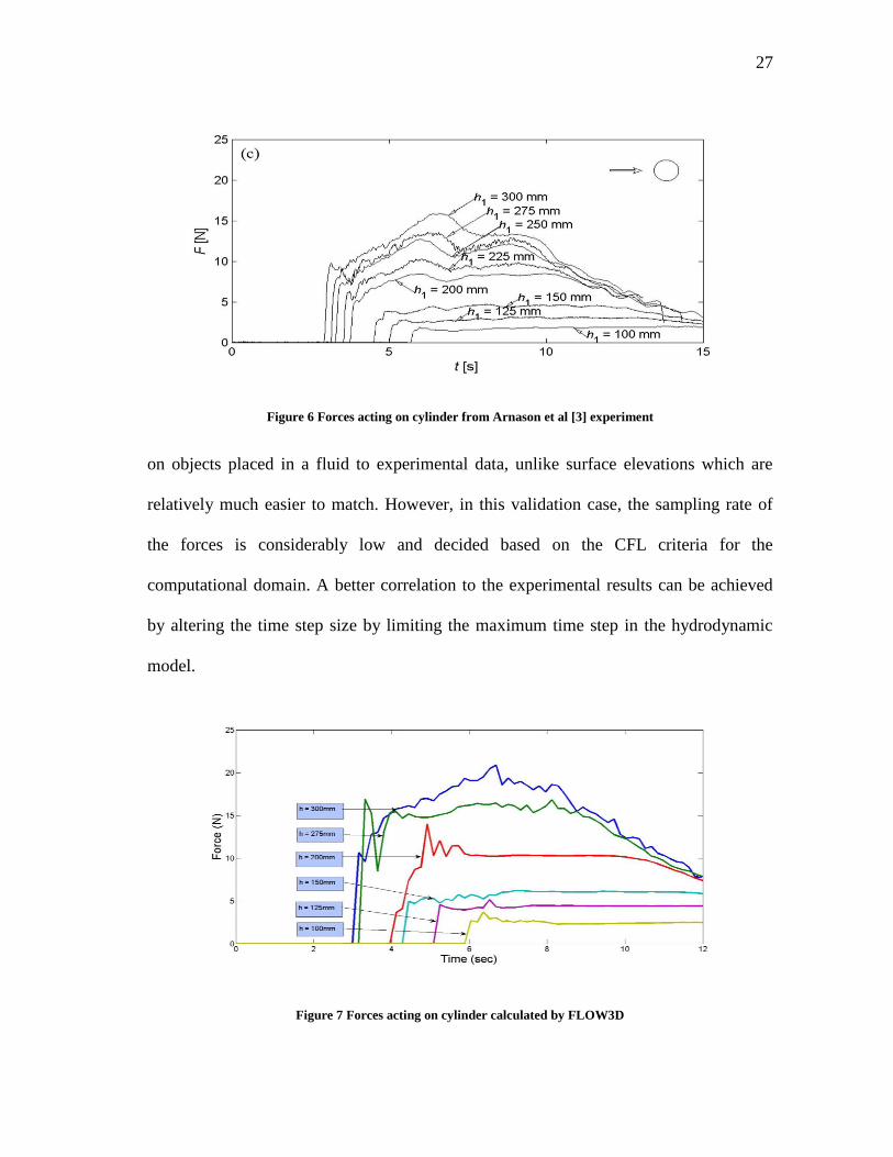
27
Figure 6 Forces acting on cylinder from Arnason et al [3] experiment
on objects placed in a fluid to experimental data, unlike surface elevations which are
relatively much easier to match. However, in this validation case, the sampling rate of
the forces is considerably low and decided based on the CFL criteria for the
computational domain. A better correlation to the experimental results can be achieved
by altering the time step size by limiting the maximum time step in the hydrodynamic
model.
Figure 7 Forces acting on cylinder calculated by FLOW3D
28
Table 2 Percentage difference in the estimation of forces (Experimental v/s Hydrodynamic model)
S.No
Impoundment
Depth
Maximum Force
Difference (%)
Experimentally(N) Numerically(N)
1 100 3.0 3.68 +22.67
2 125 3.8 4.56 +20.00
3 150 4.9 5.29 +7.95
4 200 9.8 10.50 +7.14
5 275 14.3 15.40 +7.69
6 300 18.0 19.35 +7.50
3.3 Conclusions
As observed, the hydrodynamic model only slightly overestimates the load acting on a
cylinder placed in the fluid. The overestimation of forces means that the safety of the
structure is not compromised. The overall economy of the design obviously seems to be
sacrificed, but since the probability of occurrence of the tsunami load is low it would
result in smaller safety factors on this load for design purposes and thereby neutralize the
effect of overestimation of forces. A detailed investigation of safety factor considering
hydrodynamic model uncertainty and tsunami risk is beyond the scope of this study.
Since the validation results look acceptable for the purpose of determining the forces on
the cylinder, the hydrodynamic model is used in the study to determine the forces acting
on the actual WPU tower.
29
4. QUANTIFICATION OF FORCES ON WPU
Three surge cases and three bore cases are modeled using the hydrodynamic code. A
bore/surge is usually formed after the tsunami wave is broken near the shore. A tsunami
being a long wave, the wave celerity is given by , where is the acceleration due to
gravity and is the depth of flow. The computational domain that is modeled begins
after the wave has broken and progresses through it the form of a bore/surge. Modeling
of tsunami bore/surge using the hydrodynamic model involves the following steps:
4.1 Establishing a Computational Domain
The right handed coordinate system (Figure 8) for the hydrodynamic computational
mesh is oriented such that the X- direction is directed along the fluid flow into the
domain. The Y-direction is oriented perpendicular to the direction of the flow. The Z-
direction is in the upward direction. For the purpose of determining the hydrodynamic
forces on the WPU, it is idealized as a cylinder having a diameter equal to the base of the
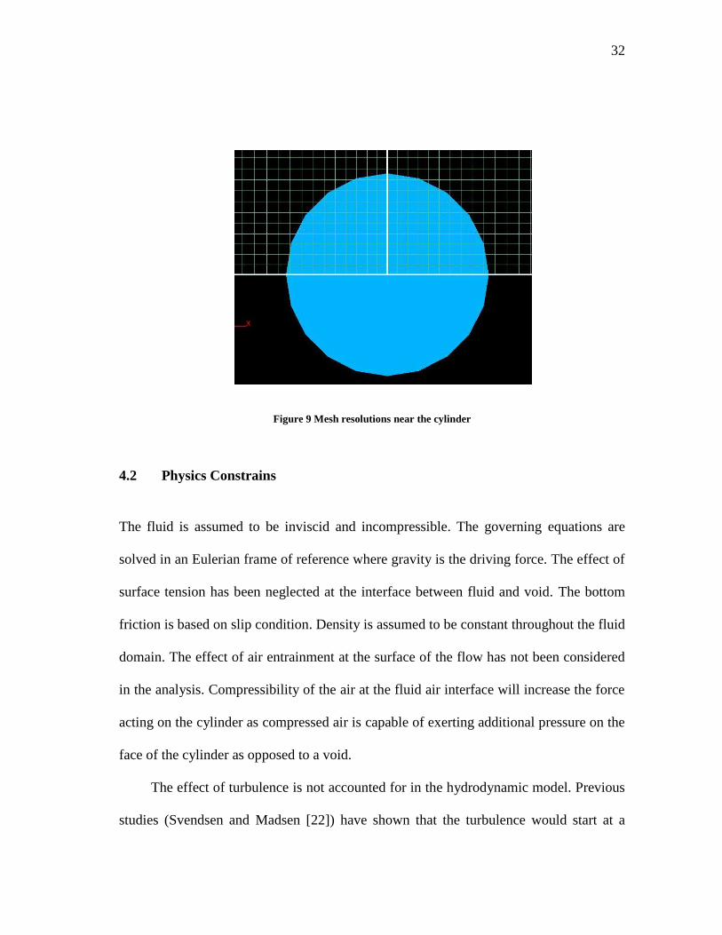
WPU tower. The cell sizes are not uniform throughout the mesh. It has finer resolution
near the face of the cylinder in the X and Y direction (Figure 9). This is because the front
of the tsunami bore is very steep just before impacting on the cylinder and smaller cells
will be capable of better capturing the pressures around the cylinder and hence force
field on the cylinder. Again reducing the cell size indefinitely doesn’t necessarily
guarantee a better result from a practical perspective as the increase in accuracy after a
specific threshold cell size isn’t worth the computational resources and time utilized for
30
carrying out the simulation. The specifications of the computational mesh for the various
surge/bore cases are given in Table 3. The flooding/upstream impoundment depths used
in the bore impact cases are shown in Table 4. The flooding depth has an impact on the
force exerted by the bore on the WPU tower. This is due to the enhancement of the
momentum flux behind the front of the bore due to the non uniform velocity profiles
within the bore (Svendsen and Madsen [22]).
Table 3 Specification of computational domain for determining forces on WPU
Case
Height
(m)
Domain Size Number of Cells Cell Size Range(m)
L (m) B (m) H (m) NX x NY x NZ DX DY DZ
Bore/
Surge
2 50 5.0 6.0 266 x 50 x 60
= 0.798 million
0.40 -
0.10
0.15 -
0.10
0.10 -
0.10
5 50.0 5.0 11.0 266 x 50 x 110
= 1.463 million
0.40 -
0.10
0.15 -
0.10
0.10 -
0.10
10 50.0 5.0 20.0 266 x 50 x 220
= 2.926 million
0.40 -
0.10
0.15 -
0.10
0.10 -
0.10
Table 4 Impoundment depth and flooding depth
S.No Impoundment Depth (m) Flooding Depth (m)
1 2 0.5
2 5 0.5
3 10 1.0
31
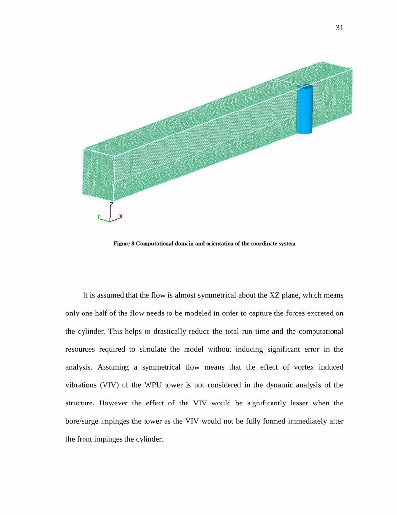
Figure 8 Computational domain and orientation of the coordinate system
It is assumed that the flow is almost symmetrical about the XZ plane, which means
only one half of the flow needs to be modeled in order to capture the forces excreted on
the cylinder. This helps to drastically reduce the total run time and the computational
resources required to simulate the model without inducing significant error in the
analysis. Assuming a symmetrical flow means that the effect of vortex induced
vibrations (VIV) of the WPU tower is not considered in the dynamic analysis of the
structure. However the effect of the VIV would be significantly lesser when the
bore/surge impinges the tower as the VIV would not be fully formed immediately after
the front impinges the cylinder.
32
Figure 9 Mesh resolutions near the cylinder
4.2 Physics Constrains
The fluid is assumed to be inviscid and incompressible. The governing equations are
solved in an Eulerian frame of reference where gravity is the driving force. The effect of
surface tension has been neglected at the interface between fluid and void. The bottom
friction is based on slip condition. Density is assumed to be constant throughout the fluid
domain. The effect of air entrainment at the surface of the flow has not been considered
in the analysis. Compressibility of the air at the fluid air interface will increase the force
acting on the cylinder as compressed air is capable of exerting additional pressure on the
face of the cylinder as opposed to a void.
The effect of turbulence is not accounted for in the hydrodynamic model. Previous
studies (Svendsen and Madsen [22]) have shown that the turbulence would start at a
33
location behind the front of a bore increases in thickness behind the front. This
turbulence would spread towards the bottom as the bore propagates. An investigation
into the variation in forces because of this is beyond the scope of this study.
4.3 Boundary Conditions
The bore/surge is input into the computational domain using a velocity equal to the wave
celerity and a fluid height equal to the bore/surge height. The inflow boundary at the
upstream end of the fluid domain is modeled using the velocity boundary condition. This
sets the fluid height in the ghost cell to the value specified by the user and the velocity
drives the flow into the domain as described by the VOF transport equations. Since our
primary interested is in the forces exerted on the cylinder, which is influenced only by
the flow field in the vicinity of the cylinder, it is not necessary to model the flow in the
downstream locations at a reasonable distance away from the cylinder. Hence the
downstream end of the fluid domain has outflow boundary condition, which permits the
flow reaching that boundary to exit the domain. This is accomplished as shown in
section 2.1.5.2. The upper boundary of the fluid domain is also modeled as an outflow
boundary condition as this helps any stray sprays/volume of water, generated by the
splashing of the fluid on the cylinder to leave the domain. These hardly influence the
forces on the cylinder, even if they are reflected from the top, but make the visual
interpretation of the flow patterns difficult. The other boundary conditions in the flow
are rigid wall boundary conditions, which do to permit any fluid to enter or exit the
domain.
34
4.4 Numerical Schemes
The time step size for the simulation is determined by the model using the stability and
convergence criterion as described in section 2.1.6. The generalized minimal residual
(GMRES) method based implicit scheme pressure solver is used to solve the momentum
equation. Momentum advection is approximated using the first order terms.
4.5 Simulation
Model simulation is carried out using both processors on a dual core computer. The
simulation time for the various surge/bore cases are shown in Table 5. The simulations
time is the real time taken by a particular case. The elapsed time is how the wall time the
computer takes to simulate the case. This includes the time taken to read input files and
generate output files. The CPU time indicates the time taken by the processors in the
actual computation and excludes the time taken for input/output tasks. The CPU time is
nearly two times the actual wall time in the cases shown below, since the hydrodynamic
model is run in parallel on two processors. The hydrodynamic model is actually scalable
up to 8 processors as long as the computer has a shared memory architecture. A shared
memory architecture is when every processor on the computer, doesn’t have its own
dedicated memory but shares a single main memory. An interesting observation here is
that the hydrodynamic model took 335600 sec (~ 3 days and 22 hours) to simulate 27.5
seconds of the 10 m bore case, which has a total of 2.9 million cells in its mesh! This is
undoubtedly a major disadvantage of using the full 3D Navier Stokes equation solver in
non parallelized systems. The simulation of flow is carried out with a time step that does
35
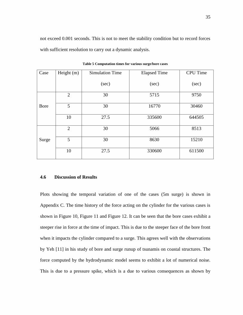
not exceed 0.001 seconds. This is not to meet the stability condition but to record forces
with sufficient resolution to carry out a dynamic analysis.
Table 5 Computation times for various surge/bore cases
Case Height (m) Simulation Time
(sec)
Elapsed Time
(sec)
CPU Time
(sec)
Bore
2 30 5715 9750
5 30 16770 30460
10 27.5 335600 644505
Surge
2 30 5066 8513
5 30 8630 15210
10 27.5 330600 611500
4.6 Discussion of Results
Plots showing the temporal variation of one of the cases (5m surge) is shown in
Appendix C. The time history of the force acting on the cylinder for the various cases is
shown in Figure 10, Figure 11 and Figure 12. It can be seen that the bore cases exhibit a
steeper rise in force at the time of impact. This is due to the steeper face of the bore front
when it impacts the cylinder compared to a surge. This agrees well with the observations
by Yeh [11] in his study of bore and surge runup of tsunamis on coastal structures. The
force computed by the hydrodynamic model seems to exhibit a lot of numerical noise.
This is due to a pressure spike, which is a due to various consequences as shown by

36
Fekken [23]. One reason is the presence of an obstruction, cutting a cell face at an angle,
which is unavoidable in case of a cylindrical object. Another cause could the air
entrainment, which occurs when a free surface impacts an object. There might be a
bubble bursting inside the fluid and this shows up as a spike and this is not unphysical.
As shown by Fekken [23], filtering these can be quite cumbersome, and this makes it
difficult to be included in this study. But since the pressures predicted by the
hydrodynamic model is pretty close to the actual results as shown in the validation and
also since these spikes do not cause any instability in the model, only a simple filtering
of the force signal, above a critical frequency of 50 Hz has been performed.
.
Figure 10 Forces on cylinder due to 2 m bore/surge

37
Figure 11 Forces on cylinder due to 5 m surge/bore
Figure 12 Forces on cylinder due to 10 m surge/bore
38
5. STRUCTURAL RESPONSE AND INTEGRITY
Once the forces exerted by the tsunami on WPU are quantified, the impact of the forces
on the WPU’s tower structure is investigated. Firstly the stresses induced by the load on
the tower structure are determined by using a simplified static analysis of the WPU. For
this, a FEM structural analysis of the cylinder is carried out using ANSYS to quantify
the stresses induced in the structure due to the hydrodynamic loads in addition to the
already existent loads on the structure. Secondly the dynamic behavior of the structure is
investigated by carrying out a simplified dynamic structural analysis of the WPU tower.
5.1 Description of WPU
The WPU tower used for this study is the 65kW Nordtank wind turbine manufactured in
Denmark. These turbines were produced in large number in the early 1980’s in
California for utility scale power generation [24] and by 1985 accounted for nearly 40%
of all wind turbines in California [24]. This turbine is much smaller than the multi mega
watt turbines of modern day, but they have more or less the same structural
configuration as the large ones. The primary reason this type of turbine is used in this
study is because University of California, San Diego has one mounted on top of a shake
table. This experimental setup can be used to determine the structural response of the
WPU under the effect of a base excitation. It is shown later that this setup can be used to
experimentally determine the dynamic response of the WPU under tsunami loading
conditions. The important characteristics of the WPU are shown in the table on page 41.

39
5.2 Static Structural Analysis
5.2.1 Numerical Modeling
The preliminary static structural analysis is carried out to determine the stresses induced
in the tower section at the point of impact of the tsunami load. The pressure field from
the hydrodynamic model is imported into the structural model to perform a structural
stress analysis.
The turbine tower is modeled as a cylinder having a diameter of 2.02 m, 5.3 mm
wall thickness and a height 15 m. The weight of structure and the components above 15
m are replaced by its weight. This is because it was observed after preliminary analyses
that the increase in stresses die down exponentially away from the point of application of
the load and extra stiffness imparted by the tower section beyond 15 m doesn’t
significantly influence the stress distribution in the cylinder, near the point of impact of
the load.
The meshing of the turbine tower in ANSYS is done using 4 noded rectangular
plate elements, which means every node is attached to exactly four elements. ANSYS’s
smart sizing option is used to automatically generate the mesh. The mesh has a
resolution of 3 mm in the X and Y direction and 0.12 m in the Z direction. The steel is
assumed to be elastic with a Young’s Modulus of 2.10x10¹¹
Pascal, with a Poisson’s
ratio of 0.29 and a density of 7850 kg/m3.
40
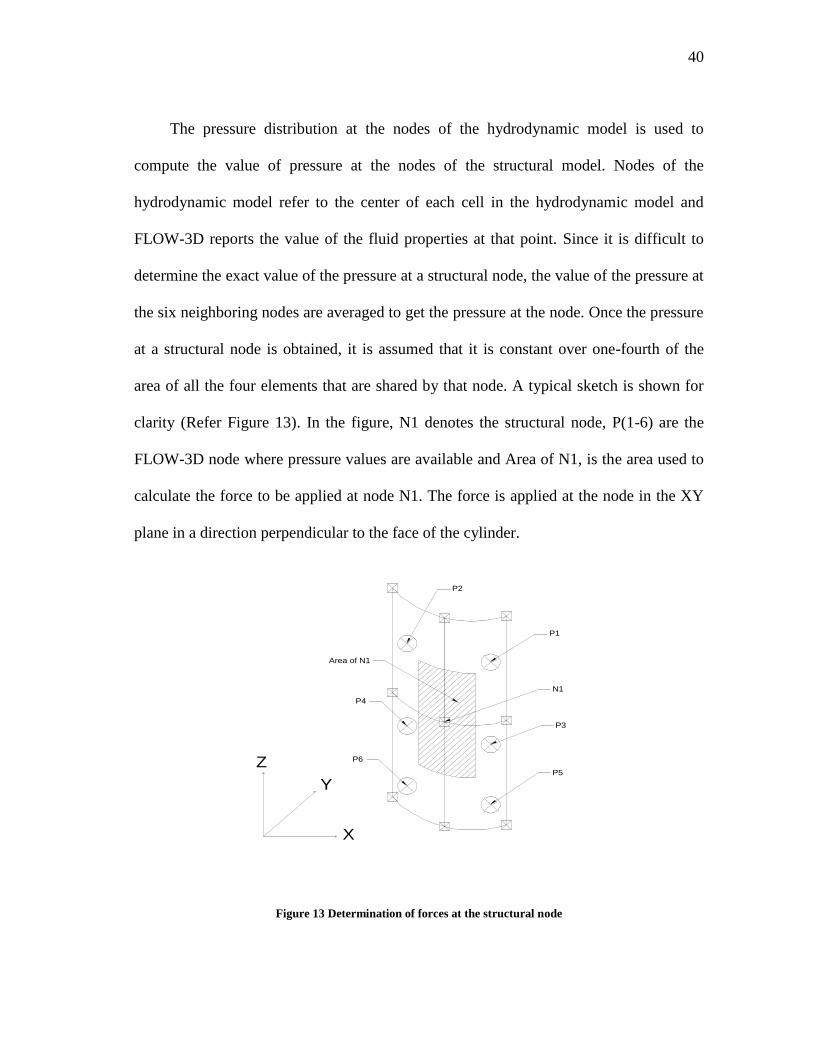
The pressure distribution at the nodes of the hydrodynamic model is used to
compute the value of pressure at the nodes of the structural model. Nodes of the
hydrodynamic model refer to the center of each cell in the hydrodynamic model and
FLOW-3D reports the value of the fluid properties at that point. Since it is difficult to
determine the exact value of the pressure at a structural node, the value of the pressure at
the six neighboring nodes are averaged to get the pressure at the node. Once the pressure
at a structural node is obtained, it is assumed that it is constant over one-fourth of the
area of all the four elements that are shared by that node. A typical sketch is shown for
clarity (Refer Figure 13). In the figure, N1 denotes the structural node, P(1-6) are the
FLOW-3D node where pressure values are available and Area of N1, is the area used to
calculate the force to be applied at node N1. The force is applied at the node in the XY
plane in a direction perpendicular to the face of the cylinder.
Figure 13 Determination of forces at the structural node
P1
P2
P3
P4
P5
P6
Area of N1
N1
Y
X
Z

41
The analyses are carried out (for the WPU described in Table 6) and the results are
shown on pages 43 to 48.
Table 6 Properties of 65kW Nordtank Turbine. Source [20]
Property Value
Rated power 65 kW
Rated wind speed 34 km/h (21 MPH)
Rotor diameter 16.0 m (628 inches)
Tower height 21.9 m (864 inches)
Lower section length 7.96 m (313 inches)
Lower section diameter 2.02 m (78 inches)
Middle section length 7.94 m (312 inches)
Middle section diameter 1.58 m (62 inches)
Top section length 6.05 m (238 inches)
Top section diameter 1.06 m (41 inches)
Tower wall thickness 5.3 mm (0.20 inches)
Rotor hub height 22.6 m (888 inches)
Tower mass 6400 kg (14 kips)
Nacelle mass 2400 kg (5 kips)
Rotor mass (with hub) 1900 kg (4 kips)
5.2.2 Discussion of Results
It is observed that the Von Mises Stress is higher in the case of a bore impact, as is
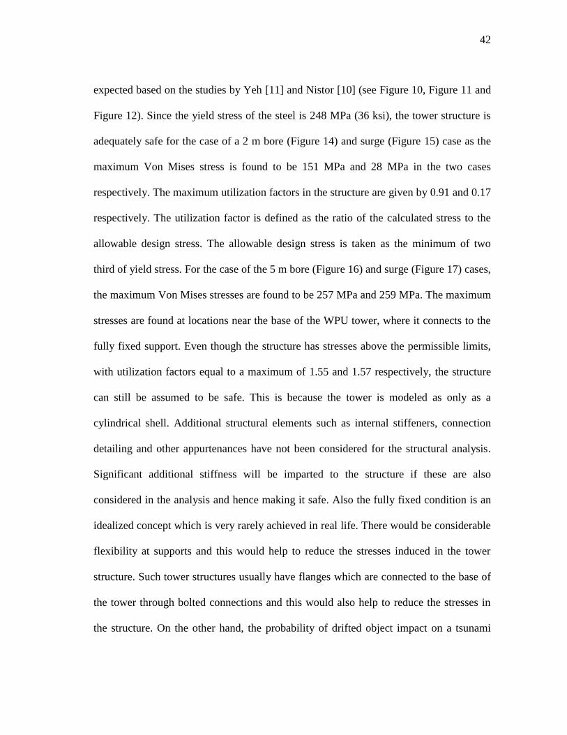
42
expected based on the studies by Yeh [11] and Nistor [10] (see Figure 10, Figure 11 and
Figure 12). Since the yield stress of the steel is 248 MPa (36 ksi), the tower structure is
adequately safe for the case of a 2 m bore (Figure 14) and surge (Figure 15) case as the
maximum Von Mises stress is found to be 151 MPa and 28 MPa in the two cases
respectively. The maximum utilization factors in the structure are given by 0.91 and 0.17
respectively. The utilization factor is defined as the ratio of the calculated stress to the
allowable design stress. The allowable design stress is taken as the minimum of two
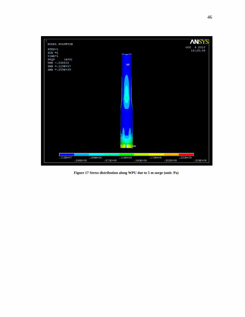
third of yield stress. For the case of the 5 m bore (Figure 16) and surge (Figure 17) cases,
the maximum Von Mises stresses are found to be 257 MPa and 259 MPa. The maximum
stresses are found at locations near the base of the WPU tower, where it connects to the
fully fixed support. Even though the structure has stresses above the permissible limits,
with utilization factors equal to a maximum of 1.55 and 1.57 respectively, the structure
can still be assumed to be safe. This is because the tower is modeled as only as a
cylindrical shell. Additional structural elements such as internal stiffeners, connection
detailing and other appurtenances have not been considered for the structural analysis.
Significant additional stiffness will be imparted to the structure if these are also
considered in the analysis and hence making it safe. Also the fully fixed condition is an
idealized concept which is very rarely achieved in real life. There would be considerable
flexibility at supports and this would help to reduce the stresses induced in the tower
structure. Such tower structures usually have flanges which are connected to the base of
the tower through bolted connections and this would also help to reduce the stresses in
the structure. On the other hand, the probability of drifted object impact on a tsunami
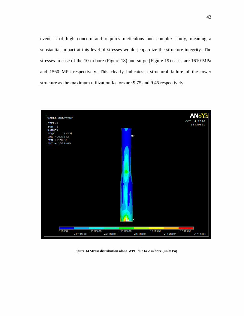
43
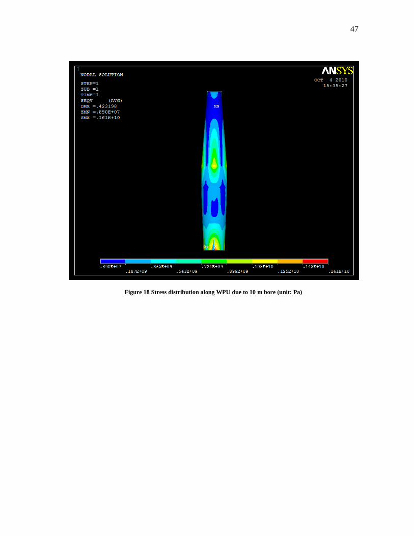
event is of high concern and requires meticulous and complex study, meaning a
substantial impact at this level of stresses would jeopardize the structure integrity. The
stresses in case of the 10 m bore (Figure 18) and surge (Figure 19) cases are 1610 MPa
and 1560 MPa respectively. This clearly indicates a structural failure of the tower
structure as the maximum utilization factors are 9.75 and 9.45 respectively.
Figure 14 Stress distribution along WPU due to 2 m bore (unit: Pa)

44
Figure 15 Stress distribution along WPU due 2 m surge (unit: Pa)

45
Figure 16 Stress distribution along WPU due to 5m bore (unit: Pa)
46
Figure 17 Stress distribution along WPU due to 5 m surge (unit: Pa)
47
Figure 18 Stress distribution along WPU due to 10 m bore (unit: Pa)

48
Figure 19 Stress distribution along WPU due to 10 m surge (unit: Pa)

49
5.3 Dynamic Structural Analysis
The dynamic structural analysis mainly tries to understand how the tsunami load would
try to dynamically excite the structure. The WPU is a multi degree of freedom system
which is quite complex to analyze. A unique feature of a WPU structure is the
gyroscopic moment generated by the rotation of its blades. At the instant of tsunami
impact, the tower will start vibrating and this vibration could meaningfully interact with
the gyroscopic moment. However, this form of a coupled analysis is beyond the scope of
this study. This study tries to determine the response generated by the tsunami load at
the different points along the WPU neglecting the effect of the gyroscopic moment. It is
assumed that the blades of the WPU are in a parking position at the time of tsunami
impact, which is not always necessarily true, but simplifies the study.
The dynamic analysis of the WPU is carried out using structural software SACS,
which will hence forth be referred to as structural analysis model Beam elements are
used to model the WPU. The structural model is made up of 3 different cylindrical
sections, the radius and thickness of each section are given in Table 6 (Page 41). The
transitions between the cylindrical sections are made with conical sections. The nacelle
and the rotors are idealized as masses and applied at the hub height. The tsunami load is
a transient load and the capability of structural analysis model to handle time history
forcing is utilized to solve the problem. The structural analysis model however accepts
the time history forcing at one node and since the point of application of the force keeps
varying with time, the net force acting at any instant on the WPU is transferred to a node

50
just above the base of the WPU by converting it to an equivalent force and moment.
Figure 20 shows how the force is transferred to the lower most nodes, here is the
load exerted by the tsunami at time t and Z (t) is the vertical coordinate of the point of
application of the load. and denotes the equivalent moment applied
at the node which is distance from the base of the WPU.
Figure 20 Force transformation
For carrying out the dynamic analysis, the first step is the generation of the mode
shapes or Eigenvectors and Eigen values or natural periods of the structure. In this case,
the tower is discretized into 30 nodes and since each node has 3 degrees of freedom in
Fx(t)
Z(t)Fx_eq(t)
Mz_eq(t)
d1
51
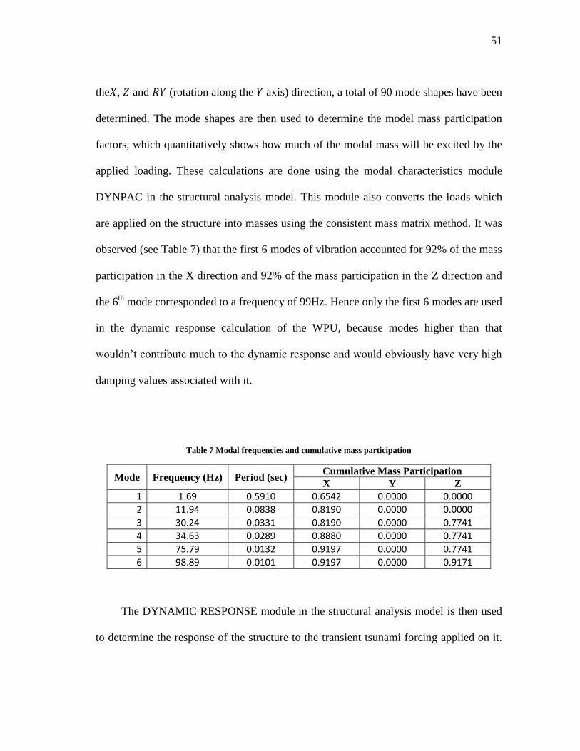
the , and (rotation along the axis) direction, a total of 90 mode shapes have been
determined. The mode shapes are then used to determine the model mass participation
factors, which quantitatively shows how much of the modal mass will be excited by the
applied loading. These calculations are done using the modal characteristics module
DYNPAC in the structural analysis model. This module also converts the loads which
are applied on the structure into masses using the consistent mass matrix method. It was
observed (see Table 7) that the first 6 modes of vibration accounted for 92% of the mass
participation in the X direction and 92% of the mass participation in the Z direction and
the 6th
mode corresponded to a frequency of 99Hz. Hence only the first 6 modes are used
in the dynamic response calculation of the WPU, because modes higher than that
wouldn’t contribute much to the dynamic response and would obviously have very high
damping values associated with it.
Table 7 Modal frequencies and cumulative mass participation
Mode Frequency (Hz) Period (sec) Cumulative Mass Participation
X Y Z
1 1.69 0.5910 0.6542 0.0000 0.0000
2 11.94 0.0838 0.8190 0.0000 0.0000
3 30.24 0.0331 0.8190 0.0000 0.7741
4 34.63 0.0289 0.8880 0.0000 0.7741
5 75.79 0.0132 0.9197 0.0000 0.7741
6 98.89 0.0101 0.9197 0.0000 0.9171
The DYNAMIC RESPONSE module in the structural analysis model is then used
to determine the response of the structure to the transient tsunami forcing applied on it.
52
This module uses the modal participation factors to redistribute the applied force along
the structure and determines the net response of the various points on the structure.
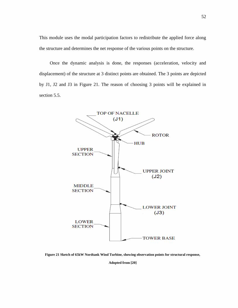
Once the dynamic analysis is done, the responses (acceleration, velocity and
displacement) of the structure at 3 distinct points are obtained. The 3 points are depicted
by J1, J2 and J3 in Figure 21. The reason of choosing 3 points will be explained in
section 5.5.
Figure 21 Sketch of 65kW Nordtank Wind Turbine, showing observation points for structural response,
Adopted from [20]
53
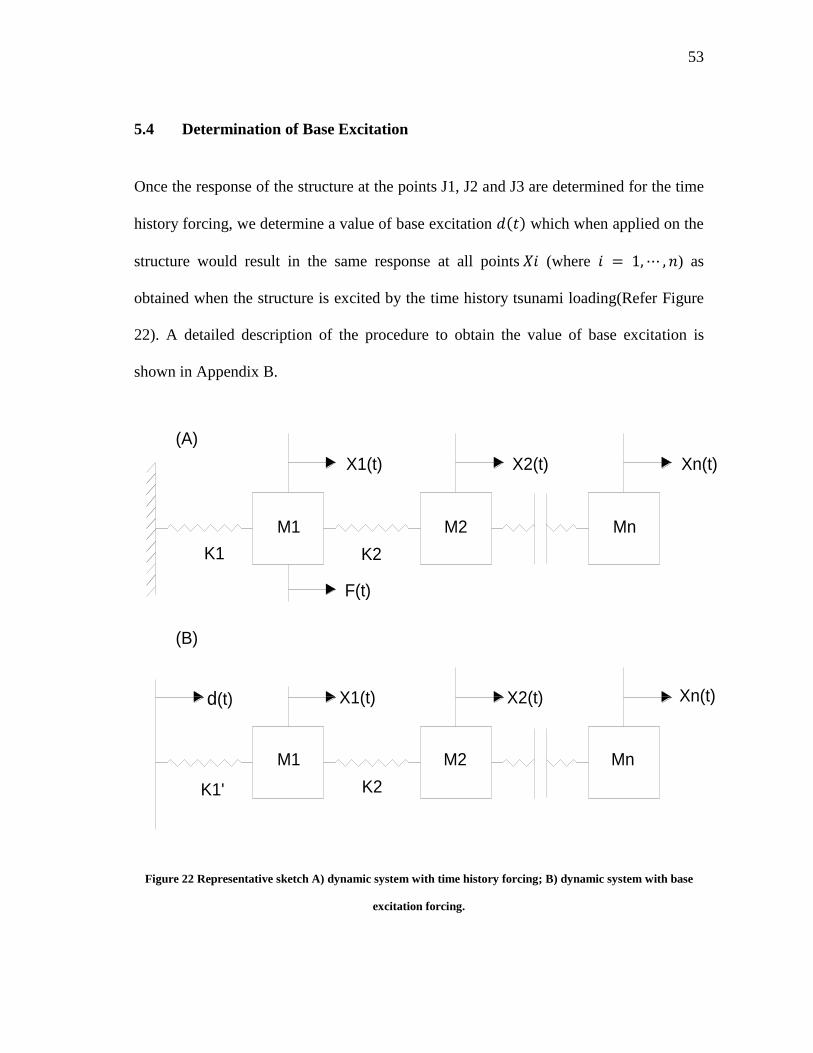
5.4 Determination of Base Excitation
Once the response of the structure at the points J1, J2 and J3 are determined for the time
history forcing, we determine a value of base excitation which when applied on the
structure would result in the same response at all points (where ) as
obtained when the structure is excited by the time history tsunami loading(Refer Figure
22). A detailed description of the procedure to obtain the value of base excitation is
shown in Appendix B.
Figure 22 Representative sketch A) dynamic system with time history forcing; B) dynamic system with base
excitation forcing.
M1 M2 Mn
M1 M2 Mn
K1' K2
K1 K2
F(t)
X1(t) X2(t) Xn(t)
d(t) X1(t) X2(t) Xn(t)
(A)
(B)
54
5.5 Base Excitation of WPU
University of California, San Diego (UCSD) owns an experimental facility which
consists of a Large High Performance Outdoor Shake Table (LHPOST). The LHPOST is
capable of imparting uniaxial horizontal excitations to structures placed on it. LHPOST
has an advantage that it is an open facility and the height of the structure that can be
placed on the shake table is not restricted. This allows the full extent of a wind turbine
tower to be tested using this shake table. UCSD also has a Nordtank 65kW wind turbine
which can be used for experimental studies and is or could be mounted on top of the
LHPOST. The primary purpose of this experimental setup is to study the impact of
earthquake loading on WPUs. The shake table is used to impart a random base excitation
to the WPU structure. Accelerometers are located at points J1, J2 and J3 shown in the
Figure 21, to determine the response of the structure to this random loading.
If the tsunami load is also converted to an equivalent base excitation, it is possible
to use the same experimental setup to study the effect of these loads on WPU towers.
This study carries out only simplified analyses of WPU structure, with assumptions such
as: 1- the blades are in parked position; and 2-only the WPU tower has dynamic degrees
of freedom. These are seldom satisfied in real life, as the blades of the WPU rotate
during operational condition and also the WPU has degrees of freedom at joints where
the rotor meets the nacelle, where nacelle meets the WPU tower along yaw axis, etc.
Once these studies are done, this same experimental setup can be used to determine the
response of the WPU under the effects of other complex loading (such as gyroscopic
55
moments, wind loading, etc.) with the participation of the full degrees of freedom of the
structure.
5.6 Results and Discussions
Figure 32 to Figure 46 (Appendix D) show the responses of the structure at points J1, J2
and J3 due to the tsunami loading in the time domain. For clarity, the spectral
components of the accelerations at joint J1 (Figure 23), J2 (Figure 24) and J3 (Figure 25)
are shown for the 5m bore/surge case. It is observed that the structure is excited mainly
at the first three natural frequencies of the structure, i.e. 1.7 Hz, 11.94 Hz and 30.24 Hz.
It is also observed that the higher modes of vibration created excitations at the lower
joints, which can be seen in Figure 23, where most of the spectral energy is located at
30.24 Hz, where as in Figure 25, most of the spectral energy is situated at 1.7 Hz. This
tells us that the higher modes would excite the masses near the point of application of
the load, these are damped out at the higher points of the structure.
The deflections of the tip of the WPU in the case studied here are found to be
negligibly small. This is attributed to the fact that the natural frequencies of the smaller
and sturdy tower are considerably high. Whereas present day WPUs which are nearly
100 m tall and slender would have lower natural periods which can be more easily
excited as there is considerably lesser damping at these frequencies. This would result in
higher deflections at the tip of the WPU tower, which would meaningfully interact with
the rotor and nacelle dynamics. This also could result in substantial loads in the WPU
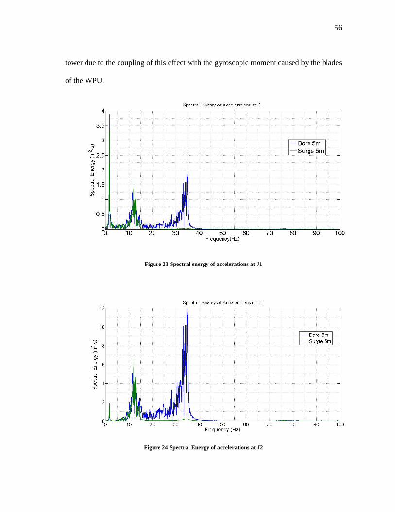
56
tower due to the coupling of this effect with the gyroscopic moment caused by the blades
of the WPU.
Figure 23 Spectral energy of accelerations at J1
Figure 24 Spectral Energy of accelerations at J2
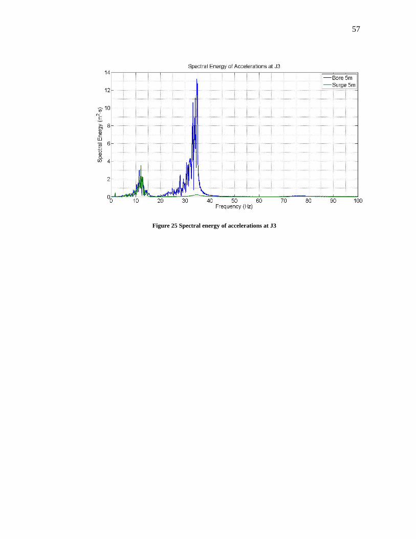
57
Figure 25 Spectral energy of accelerations at J3
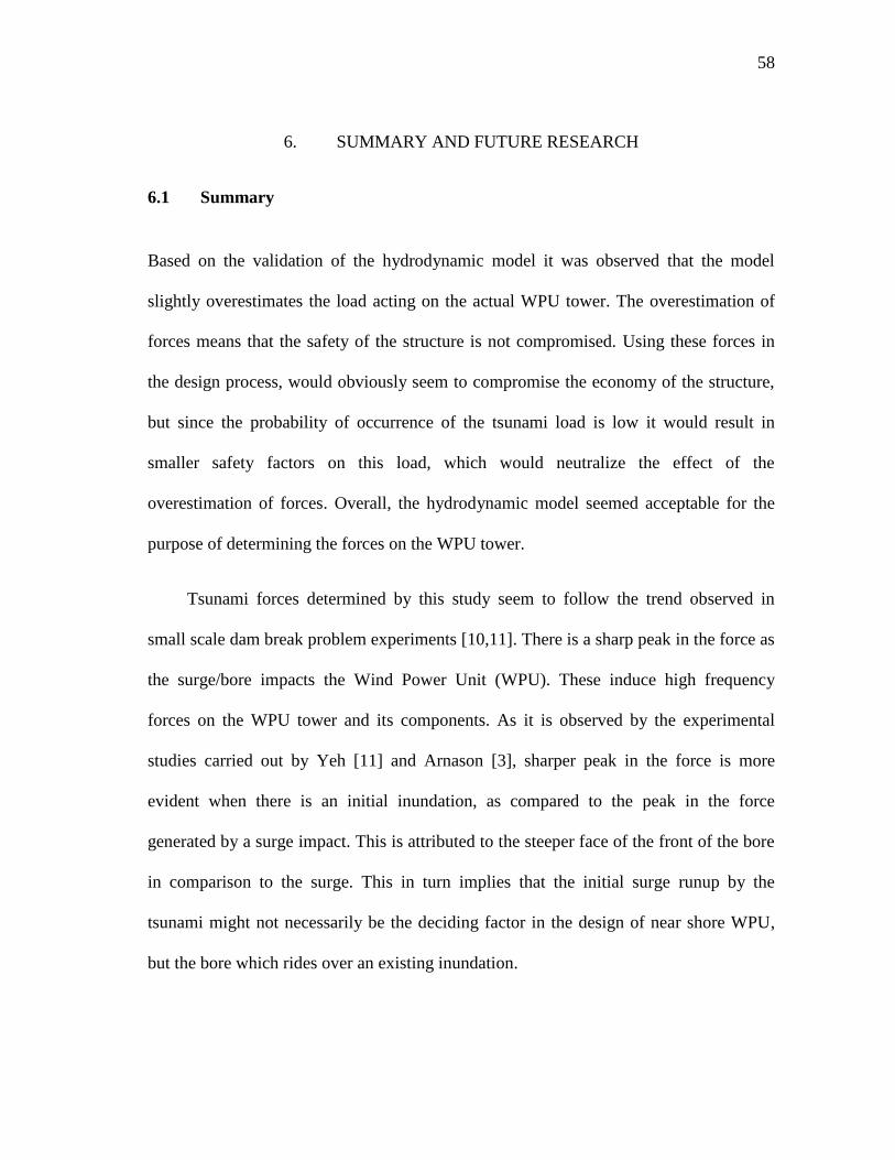
58
6. SUMMARY AND FUTURE RESEARCH
6.1 Summary
Based on the validation of the hydrodynamic model it was observed that the model
slightly overestimates the load acting on the actual WPU tower. The overestimation of
forces means that the safety of the structure is not compromised. Using these forces in
the design process, would obviously seem to compromise the economy of the structure,
but since the probability of occurrence of the tsunami load is low it would result in
smaller safety factors on this load, which would neutralize the effect of the
overestimation of forces. Overall, the hydrodynamic model seemed acceptable for the
purpose of determining the forces on the WPU tower.
Tsunami forces determined by this study seem to follow the trend observed in
small scale dam break problem experiments [10,11]. There is a sharp peak in the force as
the surge/bore impacts the Wind Power Unit (WPU). These induce high frequency
forces on the WPU tower and its components. As it is observed by the experimental
studies carried out by Yeh [11] and Arnason [3], sharper peak in the force is more
evident when there is an initial inundation, as compared to the peak in the force
generated by a surge impact. This is attributed to the steeper face of the front of the bore
in comparison to the surge. This in turn implies that the initial surge runup by the
tsunami might not necessarily be the deciding factor in the design of near shore WPU,
but the bore which rides over an existing inundation.
59
The structural stress analysis of the 65kW Nordtank WPU tower showed that it is
safe for tsunami surge/bores up to 5m. The maximum utilization factors in case of the
bore/surge of 2m are found to be less than 1. In case of the 5m surge/bore, the maximum
utilization factors are marginally above 1. The maximum utilization ratios are exceeded
near the supports of the WPU tower. Nevertheless the structure is still assumed to be
safe as the connection detailing between the tower and the structure support, which has
not been considered in the structural stress analysis, imparts additional load bearing
capacity to the structure. The connection could indeed provide adequate flexibility at the
joint in the actual configuration, relieving the stresses induced in the structure at that
point. It has been determined that a severe tsunami which has surge/bore heights of more
than 5m can damage the integrity of the structure.
The base excitation values which can be used as an input to carry out experimental
validation of the response of the WPU tower to tsunami loading has been determined.
This can be used by the experimental setup at University of California San Diego
(UCSD) to study the response of a WPU to tsunami loading.
The study however does not include the effect of impact by drifted debris.
Quantifying and studying the impact of these would pose a complex problem, which is
beyond the scope of this study.
6.2 Future Recommendations
6.2.1 Response of MDOF Turbine Model
In this particular study the dynamic response of the wind turbine tower is only looked at.
60
The other components of the WPU such as hub, the rotor, nacelle and the weight are
approximated as masses, the dynamic behaviour of which does not contribute to the
dynamics of the WPU tower. But this assumption is not entirely valid as the WPU tower
is actually a multiple degree of freedom system where the dynamics of the above
mentioned parts can dynamically couple with dynamics behaviour of the tower. The hub
motions and the gyroscopic moment associated with the blades of the wind turbine can
induce substantial dynamic excitation and hence stresses in the tower. For example, a
rotational displacement, about an axis parallel to the axis of the axle of turbine can
induce a high gyroscopic moment on the wind turbine tower. This might be capable of
compromising the structural integrity of the wind turbine tower. Some of the existing
models like FAST(NREL), ADAMS can analyse the structure accounting for a lot more
degrees of freedom, than SACS. Carrying out numerical studies using these models
would help to better understand the whole system dynamic and the stresses induced by
the gyroscopy effect on the tower.
6.2.2 Effect on Components
The initial impact of the tsunami bore/surge is capable of inducing high frequency
motions in the WPU structure. This could induce high impulsive forces on the critical
components of the WPU, such as yaw controllers, drivetrain shaft, etc. This can result in
the failure of these critical components, which can impair the functionality of the WPU.
61
6.2.3 Experimental Validation
There is a necessity for experimental validation of the structural response of a wind
turbine. This is because the damping for this system due to a tsunami excitation loading
is not yet fully understood. Hence it is proposed to perform experimental validation of
the reponses obtained using this study. The experimental setup at UCSD [21], would be
a viable way to carry out experimental validation of this study.
It is also proposed to carry out experimental validation on taller (slender) wind
turbines as the higher modes of vibration will have higher mass excitation factors, which
will result in response at the higher modes since the loading has substantial energy at
those frequencies. But carrying out such a study does pose a lot of practical issues, such
as the economics involved in the availabilty of such a WPU purely for carrying out
experimental studies. It is also not easy to mount such a large turbine on top of a shake
table. The force needed to excite a heavier turbine would also be considerably higher and
the frequency of the force that can be applied would be limited. Another alternative
might be to carry out the test using scaled models, which can easily and economically
vaildate the coupled effect of the gyroscopic moments due to the blades on the WPU
tower.
6.3 Conclusions
The forces acting on the cylinder which are determined using the hydrodynamic
model are in fair comparison to the values obtained from experimental studies.

62
The plots of the time series of the force acting on the full scale WPU tower for
surge/bore cases of 2 m, 5 m and 10 m have been obtained.
Tsunami bores caused due to an initial inundation exert more forces compared to
the initial runup or surge and hence becomes critical for structural design
purposes.
The structural responses (accelerations, velocities and displacement) of the
various points along the WPU tower have been determined.
The structural responses of the 22m WPU tower are found to be considerably
small. However it is predicted that the values would be significantly higher in
case of the present day, multi megawatt WPU towers, which at times would be in
excess of 100 m tall.
The stresses induced on the structure due to the tsunami load have been
determined and it have been identified that surge/bore in excess of 5m can result
in the failure of the WPU tower.
The base excitation values which can be used to determine the response of a
65kW Nordtank WPU mounted on a shake table have been developed.
63
REFERENCES
1. Dunbar, Paula K, Weaver, Craig S. U.S. states and territories national tsunami hazard
assessment : Historical record and sources for Waves. Technical Report National
Tsunami Hazard Mitigation Program, 2008.
2. Arnason H, Petroff C, Yeh H. Tsunami bore impingement onto a vertical column.
Journal of Disaster Research 2009; 4(6):391-403
3. Arnason H. Interactions between an incident bore and a free-standing coastal
structure. PhD dissertation University of Washington, 2005.
4. Ramsden JD. Tsunamis: Forces on a vertical wall caused by long waves, bores and
surges on a dry bed. PhD Thesis California Institute of Technology, Pasadena, 1993.
5. Chanson H, [ed.] Jun BH, Lee SI, Seo IW, Choi GW. Analytical solution of dam
break wave with flow resistance application to tsunami surges. Proceedings of the
31st IAHR Biennial Congress. 31st IAHR Biennial Congress Seoul, Korea, 11-17
September, 2005; 3341-3353
6. Davletshin V, Lappo DD. Tsunami forces exerted on vertical cylindrical barriers.
Fluid Mechanics - Soviet Research 1986; 15(3):137-147
7. Horrillo JJ. Numerical Method for Tsunami Calculation using Full Navier Stokes
Equations and Volume of Fluid Method. PhD Thesis University of Alaska Fairbanks,
Fairbanks, Alaska 2006.
8. Synolakis C. The runup of solitary waves. Journal of Fluid Mechanics 1987; 185:523-
545
9. Weihua M, Irschik K, Oumeraci H, Philip LFL. A 3D Numerical Model for
Computing Non-Breaking Wave Forces on Slender Piles. Journal of Engineering
Mathematics 2007; 58(1-4):19-30

64
10. Nistor I, Nouri Y, Palmero D, Cornett A. Experimental investigation of the impact of
a tsunami-induced bore on structures. 31st International Conference on Coastal
Engineering, Hamburg, Germany, September 2008; 3324-3336
11. Yeh, H. Design tsunami forces on onshore structures. Journal of Disaster Research
2007; 2(6):531-536.
12. Nichols BD, Hirt CW Hotchkiss RS. SOLA-VOF: A solution algorithm for transient
fluid flow with multiple free boundaries. Technical Report LA-8355 Los Alamos,
New Mexico, Los Alamos Scientific Laboratory, University of California, 1980.
13. Ngo N, Haritos T, Mendi P. Evaluating tsunami wave forces on structures.
International Symposium Disaster Reduction on Coasts 2005, Scientific-Sustainable-
Holistic-Accessible, Melbourne, Australia
14. Chorin AJ. Numerical solution of the Navier-Stokes equations. Journal of
Mathematical Computation 1968; 22: 745-762.
15. Harlow FH, Welch JE. Numerical calculation of time-dependent viscous
incompressible flow of fluid with a free surface. The Physics of Fluids 1965; 8:
2182-2189.
16. Gerrits J, Dynamics of liquid-filled spacecraft. Numerical simulation of coupled
solid-liquid. PhD Thesis University of Groningen, Groningen, Netherlands, 2001.
17. Sicilian JM, Hirt CW, An efficient computational scheme for tracking contaminant
concentrations in fluid flows. Journal of Computational Physics 1984;56:428-447.
18. Gentry RA, Martin RE, Daly BJ. An eulerian differencing method for unsteady
compressible flow problems. Journal of Computational Physics 1966;1:87-118.
19. Hirt CW, Nicholes BD. Volume of fluid method for the dynamics of free boundaries.
Journal of Computational Physics 1981; 39:201-225.

65
20. Prowell I, Veletzob M, Elgamal A, Restrepo J. Experimental and numerical seismic
response of a 65 kW wind turbine. Journal of Earthquake Engineering 2009;
13(8):1172 - 1190
21. Clough RW, Penzien J. Dynamics of Structures. McGraw-Hill New York, 1975.
22. Svendsen IA, Madsen PA. A turbulent bore on a beach. Journal of Fluid Mechanics
1984; 148: 73-96.
23. Fekken G. Numerical simulation of free-surface flow with moving rigid bodies. PhD
Thesis University of Groningen, 2004.
24. Hau E. Wind Turbines. Springer-Verlag New York, 2006.
25. Inside a wind turbine, parts explained. Top Alternative Energy Sources. Alternative
Energy for Our Future. [Online] October 1, 2010. [Cited: October 1, 2010.]
http://www.top-alternative-energy-sources.com/inside-a-wind-turbine.html.
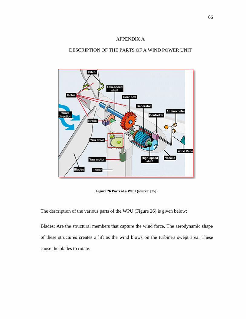
66
APPENDIX A
DESCRIPTION OF THE PARTS OF A WIND POWER UNIT
Figure 26 Parts of a WPU (source: [25])
The description of the various parts of the WPU (Figure 26) is given below:
Blades: Are the structural members that capture the wind force. The aerodynamic shape
of these structures creates a lift as the wind blows on the turbine's swept area. These
cause the blades to rotate.
67
Nacelle: Is the part that sits atop the tower and contains the gear box, low- and high-
speed shafts, generator, controller, and brake. Some nacelles are large enough for a
helicopter to land on.
Hub: Is the structural member that acts as a connection between the blades of the wind
turbine
Rotor: The assembly of the blades and the hub together is called the rotor.
Tower: Are the structural members that hold the WPU up. Towers are usually made
from tubular steel, concrete, or steel lattice. As wind speed increases with height, taller
towers enable turbines to capture more energy and generate more electricity.
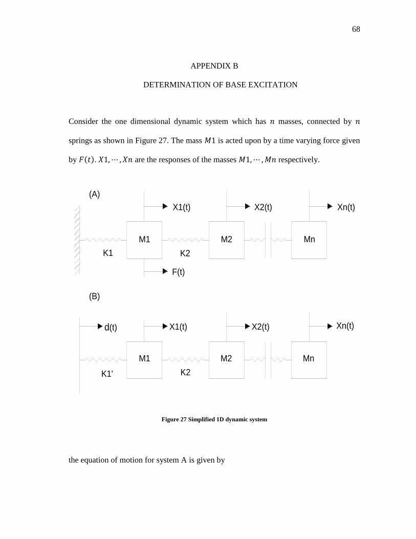
68
APPENDIX B
DETERMINATION OF BASE EXCITATION
Consider the one dimensional dynamic system which has masses, connected by
springs as shown in Figure 27. The mass is acted upon by a time varying force given
by . are the responses of the masses respectively.
Figure 27 Simplified 1D dynamic system
the equation of motion for system A is given by
M1 M2 Mn
M1 M2 Mn
K1' K2
K1 K2
F(t)
X1(t) X2(t) Xn(t)
d(t) X1(t) X2(t) Xn(t)
(A)
(B)

69
B1
where is the force along the direction due to a due to a unit displacement along the
direction. The equation of motion for system B, is given by
B2
If the responses of the masses in the two equations are equal, we get
B3
which means in order to get the base excitation we have to divide the time history of the
forcing by the stiffness of the last element. This is true only when the force is applied at
the first mass as shown. This is the reason for transferring the tsunami force acting on
the WPU to the first node above the base.
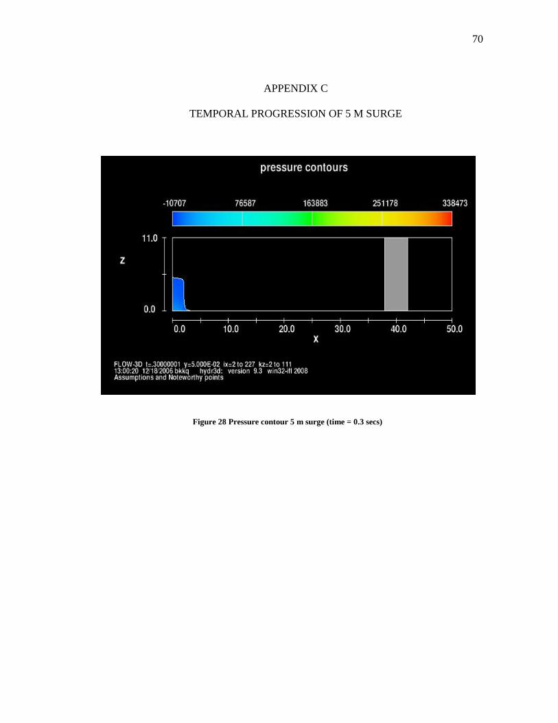
70
APPENDIX C
TEMPORAL PROGRESSION OF 5 M SURGE
Figure 28 Pressure contour 5 m surge (time = 0.3 secs)
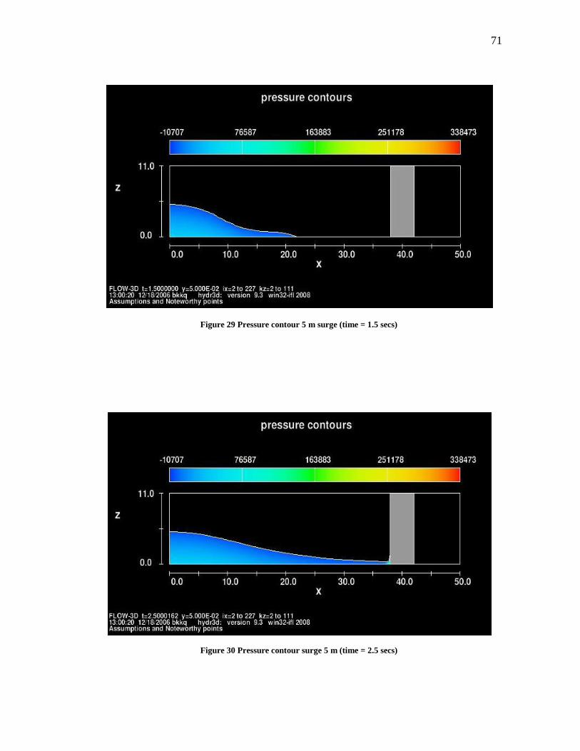
71
Figure 29 Pressure contour 5 m surge (time = 1.5 secs)
Figure 30 Pressure contour surge 5 m (time = 2.5 secs)
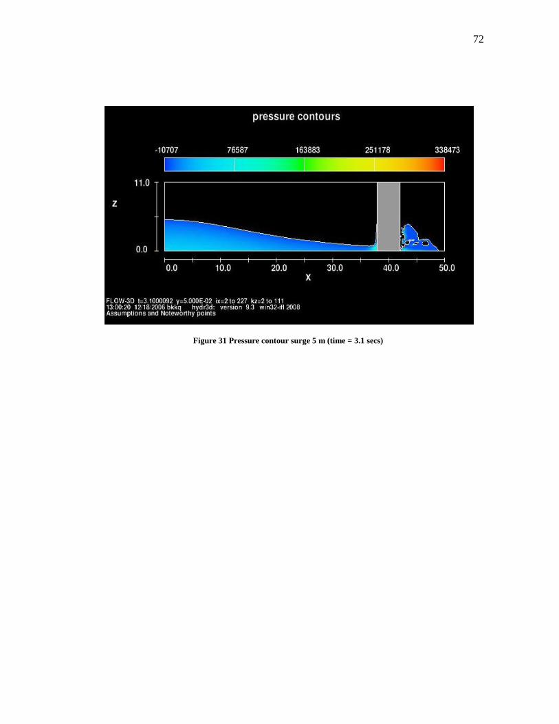
72
Figure 31 Pressure contour surge 5 m (time = 3.1 secs)
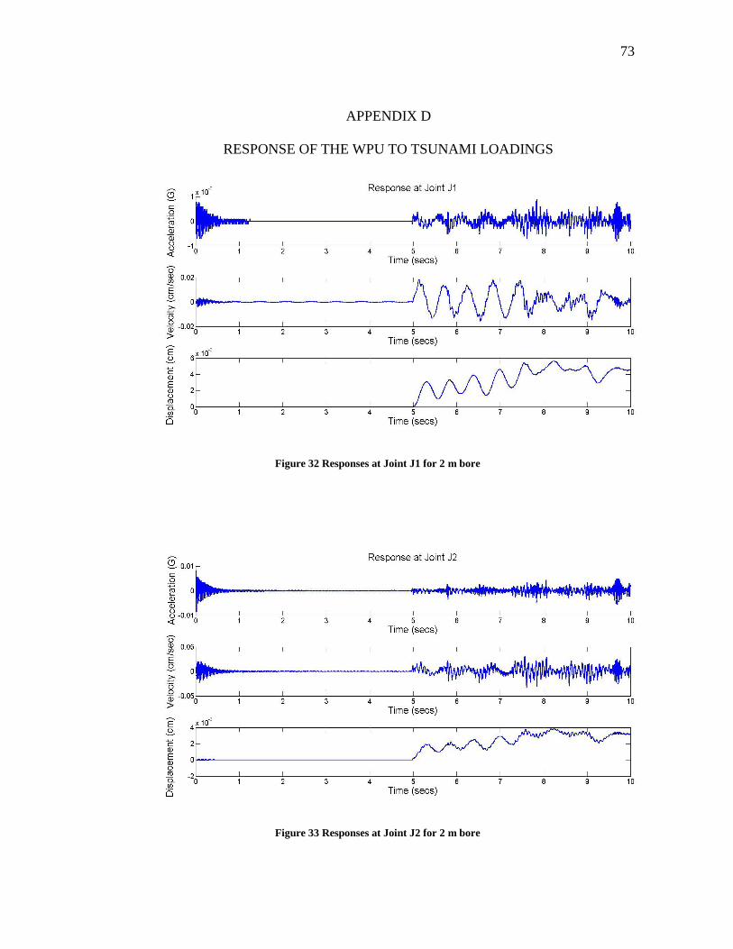
73
APPENDIX D
RESPONSE OF THE WPU TO TSUNAMI LOADINGS
Figure 32 Responses at Joint J1 for 2 m bore
Figure 33 Responses at Joint J2 for 2 m bore

74
Figure 34 Responses at Joint J3 for 2 m bore
Figure 35 Responses at Joint J1 for 2 m surge
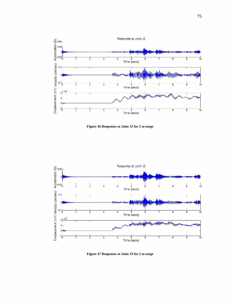
75
Figure 36 Responses at Joint J2 for 2 m surge
Figure 37 Responses at Joint J3 for 2 m surge
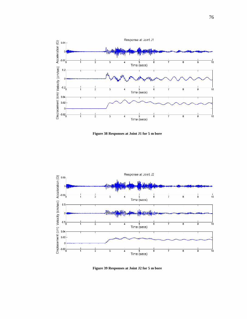
76
Figure 38 Responses at Joint J1 for 5 m bore
Figure 39 Responses at Joint J2 for 5 m bore
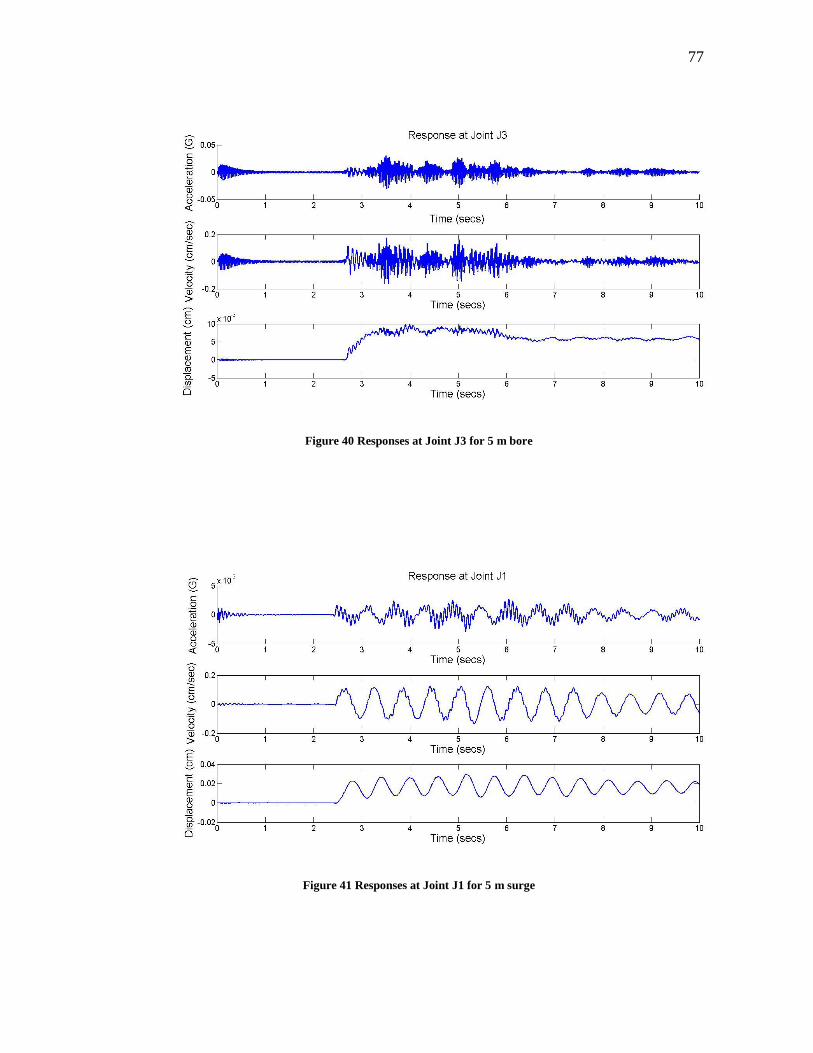
77
Figure 40 Responses at Joint J3 for 5 m bore
Figure 41 Responses at Joint J1 for 5 m surge
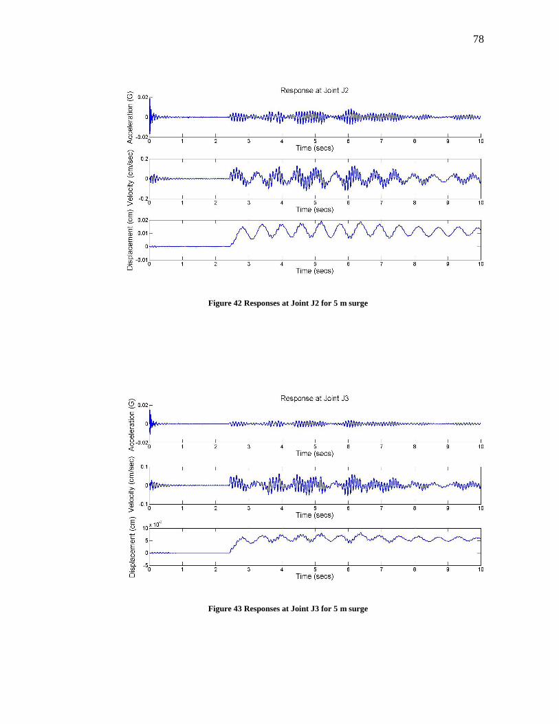
78
Figure 42 Responses at Joint J2 for 5 m surge
Figure 43 Responses at Joint J3 for 5 m surge
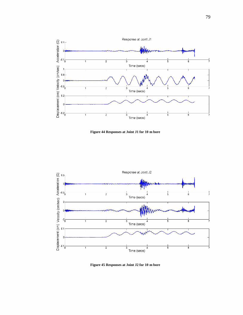
79
Figure 44 Responses at Joint J1 for 10 m bore
Figure 45 Responses at Joint J2 for 10 m bore
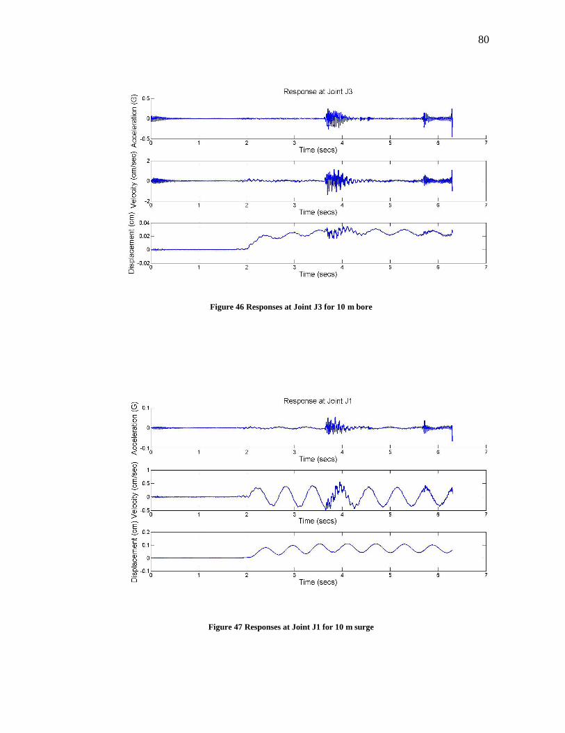
80
Figure 46 Responses at Joint J3 for 10 m bore
Figure 47 Responses at Joint J1 for 10 m surge
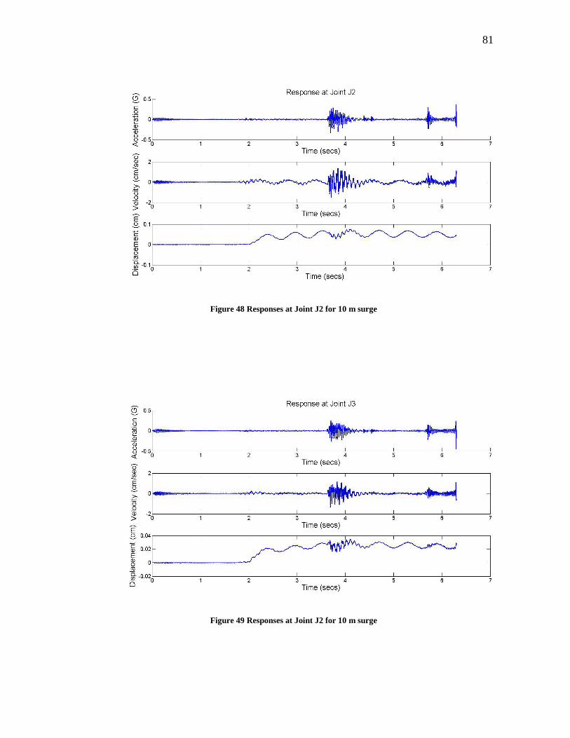
81
Figure 48 Responses at Joint J2 for 10 m surge
Figure 49 Responses at Joint J2 for 10 m surge

82
VITA
Name: Ashwin Lohithakshan Parambath
Address: Department of Civil Engineering
c/o Dr. Juan Horrillo
Texas A&M University
College Station, TX-77843-3136
Email Address: [email protected]
Education: B.Tech. (Civil), National Institute of Technology Calicut, 2006
M.S., Ocean Engineering, Texas A&M University, 2010