
Impact of the Unsteady Aerodynamics of Oscillating...
237
Universidad Politécnica de Madrid Escuela Técnica Superior de Ingenieros Aeronáuticos Impact of the Unsteady Aerodynamics of Oscillating Airfoils on the Flutter Characteristics of Turbomachines Tesis Doctoral Almudena Vega Coso Ingeniera Aeronáutica Madrid, 2016
Transcript of Impact of the Unsteady Aerodynamics of Oscillating...

Universidad Politécnica de Madrid
Escuela Técnica Superior de Ingenieros Aeronáuticos
Impact of the Unsteady Aerodynamics ofOscillating Airfoils on the
Flutter Characteristics of Turbomachines
Tesis Doctoral
Almudena Vega Coso
Ingeniera Aeronáutica
Madrid, 2016


Departamento de Mecánica de Fluidos y PropulsiónAeroespacial
Escuela Técnica Superior de Ingenieros Aeronáuticos
Impact of the Unsteady Aerodynamics of
Oscillating Airfoils on the
Flutter Characteristics of Turbomachines
AutorAlmudena Vega CosoIngeniera Aeronáutica
DirectorRoque Corral GarcíaDoctor Ingeniero Aeronáutico
Madrid, 2016

Tribunal nombrado por el Sr. Rector Magfco. de la Universidad Politécnica de
Madrid, el día ........ de ................... de 20.....
Presidente: Benigno Lázaro
Vocal: Damian Vogt
Vocal: Carlos Martel
Vocal: Mehdi Vahdati
Secretario: Manuel Antonio Burgos
Realizado el acto de defensa y lectura de la Tesis el día 1 de Diciembre de 2016 en la
Escuela Técnica Superior de Ingeniería Aeronáutica
Calificación ..............................
EL PRESIDENTE LOS VOCALES
EL SECRETARIO


You can’t connect the dots looking forward; you
can only connect them looking backwards. So
you have to trust that the dots will somehow
connect in your future.
Steve Jobs


Abstract
This thesis studies the unsteady aerodynamics of oscillating airfoils in the low reduced
frequency regime, with special emphasis on its impact on the scaling of the work per
cycle curves, using an asymptotic approach and numerical experiments.
The unsteady aerodynamics associated with the vibration of turbine and compressor
bladed-discs and stator vanes is nowadays routinely analysed within the design loop of
the aeroengine companies, and it has also been the subject of dedicated experiments.
The final aim is the derivation of the aerodynamic stability of rotor blades and the
quantification of the aerodynamic damping, which is the result of the application
of the unsteady pressures on the airfoil displacements. Little attention has been
historically paid to the understanding of vibrating airfoil aerodynamics, since this is
not a figure of merit in itself for the aeroelastic analyst, and then, little understanding
has been gained in recent years about the physics of these type of flows and its impact
on the aerodynamic damping. As a consequence, although there are several trends
that are well known by the aeroelastic community, such as the stabilisation with the
reduced frequency, or the different shape of the work per cycle curves for LPTs and
compressors, the physics which is behind this behaviour is not really well understood
and these statements lack of a sound theoretical support.
A perturbation analysis of the linearised Navier-Stokes equations for real modes at low
reduced frequency is presented and some conclusions are drawn. The first important
result is that a new parameter, the unsteady loading of the airfoil, ULP, plays an
essential role in the trends of the phase and modulus of the unsteady pressure caused
by the vibration of the airfoil. This parameter depends solely on the steady flow-field
i
on the airfoil surface and the vibration mode-shape. As a consequence, the effect of
changing the design operating conditions or the vibration mode onto the work-per-
cycle curves (and therefore onto the stability) can be easily predicted and, what is
more important, quantified without conducting additional flutter analysis.
For lightly unsteady loaded airfoils, the unsteady pressure and the influence
coefficients scale linearly with the reduced frequency whereas the phase departs from
π/2 and changes linearly with the reduced frequency. As a consequence, the work-per-
cycle scales linearly with the reduced frequency for any inter-blade phase angle, and it
is independent of its sign (the work-per-cycle curves are symmetric with respect inter-
blade phase angle zero, even for an asymmetric cascade, which is a surprising effect).
For highly unsteady loaded airfoils, the unsteady pressure modulus is fairly constant
exhibiting only a small correction with the reduced frequency, while the phase departs
from zero and varies linearly with it. In this case only the mean value of the work-
per-cycle scales linearly with the reduced frequency. This behavior is independent
of the geometry of the airfoil and the modeshape in first order approximation in the
reduced frequency. For symmetric cascades the work-per-cycle scales linearly with
the reduced frequency irrespectively of whether the airfoil is loaded or not. It is
readily concluded that for lightly unsteady loaded airfoils, or symmetric cascades, it
is not possible to change the stability by reduced frequency criterion.
These conclusions have been numerically verified on several airfoil geometries. With
this aim, simulations using a frequency domain linearised Navier-Stokes solver have
been carried out on rows of a low-pressure turbine airfoil section, the NACA65
and NACA0012 sections, and a flat plate (which is commonly considered as the
simplest representation of a compressor airfoil, and the tip of the last stages of
heavy duty land-based power turbines), to show the correlation between the actual
value of the unsteady loading parameter (ULP) and the flutter characteristics for
different airfoils, operating conditions and mode-shapes. Both, the traveling-wave
and influence coefficient formulations of the problem are used in combination to
increase the understanding of the ULP influence in different aspects of the unsteady
flow-field. It is concluded that, for a blade oscillating in a prescribed motion at
ii

design conditions, the ULP can quantitatively predict the effect of loading variations
due to changes in the incidence, and also in the mode shape. It is also proved that
the unsteady loading parameter can be used to compare the flutter characteristics of
different airfoils.
The beauty of the ULP derived in the present thesis is that it is able to account
for the effect on the stability of the work-per-cycle curves of the mode-shape and
the aerodynamic loading distribution (in a quantitative way), and the geometry (in a
qualitative way), in the low reduced frequency limit, without performing any unsteady
simulation. As a consequence, the parameter is well suited for engineering conceptual
studies, since it is able to anticipate the effect of design changes in the aerodynamic
damping.
The academic implications of the findings of the present thesis are not negligible
either, since: i) it provides a theoretical support for some well-known fundamental
concepts related to the stability of oscillating blades, and ii) it introduces new
fundamental concepts, such as for example the importance of the symmetry of the
cascade, or the unteady loading parameter, which have been proved being of major
relevance in the flutter characteristics of turbomachinery blades.
iii

Resumen
Esta tesis estudia la aerodinámica no estacionaria de perfiles oscilantes, en el régimen
de frecuencia reducida baja, con especial énfasis en el impacto que esta tiene en el
escalado de las curvas de trabajo por ciclo. Con esta finalidad, se utilizarán métodos
asintóticos y experimentos numéricos.
La aerodinámica no estacionaria asociada a la vibración de turbinas y compresores,
y vanos de estator se analiza comúnmente de forma rutinaria dentro del bucle de
diseńo en las compańías de motores de aviación, y ha sido el objeto de muchos
experimentos dedicados. El objetivo final de estos esfuerzos es la derivación de
la estabilidad aerodinámica de los álabes de rotor y la cuantificación del damping
aerodinámico, que es el resultado de la aplicación de las presiones no estacionarias
sobre los desplazamientos del álabe.
Históricamente, se ha prestado poca atención a comprender la aerodinámica de
perfiles vibrantes, ya que no es una figura de mérito en sí mismo para el analista
aeroelástico y, como consecuencia, se ha ganado muy poco conocimiento en los últimos
ańos acerca de la física de este tipo de flujos, y su impacto en el damping aerodinámico.
Aunque hay ciertas tendencias que son bien conocidas por la comunidad aeroelástica,
como la estabilización con la frecuencia reducida, o la diferente forma de las curvas de
trabajo por ciclo de compresores y turbinas de baja presión; la física que está detrás
de estos comportamientos no es realmente entendida, y estas observaciones carecen
de un soporte teórico.
En la tesis se presentará un análisis de perturbaciones a baja frecuencia reducida de
las ecuaciones de Navier-Stokes linealizadas, y se derivarán conclusiones prácticas.
v

El primer resultado importante es que un nuevo parámetro, la carga aerodinámica
no estacionario del álabe (ULP por sus siglas en inglés), juega un papel esencial en
la tendencia de la fase y el módulo de la presión no estacionaria generada por la
vibración del álabe. Este parámetro depende solo del flujo base estacionario en la
superficie del álabe y de la forma modal de la vibración. Como consecuencia directa,
el efecto de cambiar las condiciones de operación de diseńo en las curvas de trabajo
por ciclo (y, por tanto, en la estabilidad) puede ser predicho fácilmente y, lo que es
más importante, cuantificado, sin realizar ningún análisis de flameo adicional.
Se concluye que, para perfiles débilmente cargados, la presión no estacionaria y los
coeficientes de influencia escalan linealmente con la frecuencia reducida, mientras
que su fase parte de π/2 y cambia linealmente con la frecuencia reducida. Como
consecuencia, el trabajo por ciclo escala linealmente con la frecuencia reducida para
cualquier valor de inter-blade phase angle, y es independiente de su signo (las curvas
de trabajo por ciclo son simétricas con respecto al inter-blade phase angle cero, incluso
cuando se considera una cascada asimétrica, lo cual es una conclusioń sorprendente).
Para perfiles altamente cargados, el módulo de la presión no estacionaria es constante,
y solamente presenta una pequeńa corrección con la frecuencia reducida, mientras que
la fase parte de cero y varía linealmente con este parámetro. En estos casos, solamente
el valor medio del trabajo por ciclo escala linealmente con la frecuencia reducida. El
comportamiento predicho por la teoría para ambos casos es en primera aproximación,
independiente de la geometría del perfil y de la forma modal de vibración. Para
cascadas simétricas, el trabajo por ciclo escala linealmente con la frecuencia reducida,
independientemente de que el perfil esté cargado o no. La consecuencia directa es que
para perfiles débilmente cargados y para cascadas simétricas, no es posible cambiar
la estabilidad de la configuración utilizando la frecuencia reducida.
Estas conclusiones se han verificado numéricamente en distintas geometrías de álabes.
Se ha realizado una campańa de simulaciones utilizando un solver lineal de las
ecuaciones de Navier-Stokes en el dominio de la frecuencia, utilizando los siguientes
perfiles: un perfil correspondiente a una turbina de baja presión, los perfiles NACA65
y NACA0012, y placa plana (que se considera representativa de la parte superior de
vi
un álabe de compresor). El objetivo final es probar que se cumplen las tendencias
predichas para la amplitud y fase de la presión no estacionaria, y para las curvas de
trabajo por ciclo, y mostrar la correlación entre el valor calculado del parámetro de
carga no estacionario (ULP) y las características en flameo para distintos perfiles,
condiciones de operación y formas modales de vibración.
Se han utilizado las formulaciones de coeficientes de influencia y de onda viajera en
combinación para aumentar la comprensión de la influencia del ULP en distintos
aspectos del campo fluido no estacionario. Se concluye que, para un álabe oscilando
con un movimiento prescrito en condiciones de diseńo, el ULP puede predecir de
forma cuantitativa el efecto de variar el loading estacionario, debido a cambios en
la incidencia, y el efecto de cambiar la forma modal. Se prueba también que el
ULP puede ser utilizado también para comparar las características en flameo entre
distintos perfiles.
La belleza del parametro de carga no estacionario derivado en la presente tesis es
que es capaz de predecir el efecto en la estabilidad de cambios en la forma modal
de vibración y en la distribución de carga aerodinámica (de forma cuantitativa),
y en la geometría del perfil aerodinámico (de forma cualitativa), en el regimen de
frecuencia reducida baja, sin realizar ninguna simulación no-estacionaria. Como
consecuencia, el parámetro es muy válido desde el punto de vista ingenieril para
estudios aerodinámicos conceptuales, ya que es capaz de predecir el efecto de cambios
en el diseńo en el damping aerodinámico.
Las implicaciones académicas tampoco son despreciables, ya que: i) aporta un soporte
teórico a algunos de los conceptos fundamentales relativos a la estabilidad de perfiles
vibrantes existentes hasta la fecha y ii) introduce una serie de conceptos nuevos, como
la importancia de la simetría de la cascada, entre otros, a los que no se había prestado
atención con anterioridad, y son de gran relevancia en las características de flameo
de perfiles de turbomaquinaria.
vii


Acknowledgments
Firstly, I would like to express my gratitude to my supervisor Dr. Roque Corral for
giving me the opportunity to perform this thesis, for his technical support throughout
my work, and for sharing with me his wide experience in many different aspects, not
only the most technical ones. Much of my knowledge on the thesis’s subject, and the
success of this work stems from his motivating teaching method.
I also gratefully acknowledge ITP S.A for providing me financial support toward
this research, and all the necessary logistic conditions to perform my work in a high
technology environment.
Special thanks to the people of the Technology and Methods Department of ITP,
they have contributed to me to get a vision of the excellence and the rigour in the
work, and they have been an example of well-done things all over these years. Last
but not least, lot of thanks to the people of the Aerodynamics Department of ITP
for their company, support, good discussions, and all the nice coffee breaks and daily
meals; they really have boosted my enthusiasm during my stay at ITP.
I would also like to thank my colleagues at the School of Aeronautics, for creating a
pleasant working environment during the last year of my thesis, and for transmitting
me all their dynamism and positive thoughts.
Special thanks go to my family, it is so difficult to express all my gratitude, for giving
me the necessary energy to succeed in this daunting task, with their unconditional
trust and infinite love.
i

Contents
1 Introduction 1
1.1 Context . . . . . . . . . . . . . . . . . . . . . . . . . . . . . . . . . . 1
1.2 Motivation . . . . . . . . . . . . . . . . . . . . . . . . . . . . . . . . . 2
1.3 Turbomachinery Aeroelasticity Background . . . . . . . . . . . . . . . 4
1.3.1 Definition . . . . . . . . . . . . . . . . . . . . . . . . . . . . . 4
1.3.2 Static Aeroelasticity . . . . . . . . . . . . . . . . . . . . . . . 5
1.3.3 Dynamic Aeroelasticity . . . . . . . . . . . . . . . . . . . . . . 6
1.3.4 Forced Response . . . . . . . . . . . . . . . . . . . . . . . . . 6
1.3.5 Flutter . . . . . . . . . . . . . . . . . . . . . . . . . . . . . . . 7
1.3.6 Non-synchronous Vibrations (NSV) . . . . . . . . . . . . . . . 12
2 Turbomachinery Aeromechanics Fundamentals 13
2.1 Simplified Aeroelastic Model . . . . . . . . . . . . . . . . . . . . . . . 13
2.1.1 Bladed-Disc Lumped Model . . . . . . . . . . . . . . . . . . . 15
2.1.2 Purely structural problem . . . . . . . . . . . . . . . . . . . . 19
2.1.3 Aerodynamic contribution . . . . . . . . . . . . . . . . . . . . 21
2.2 Formulation of the Tuned Flutter Problem . . . . . . . . . . . . . . . 24
2.2.1 Structural vibration modes . . . . . . . . . . . . . . . . . . . . 26
2.2.2 Aerodynamic correction . . . . . . . . . . . . . . . . . . . . . 28
iii
2.2.3 Influence Coefficient Formulation . . . . . . . . . . . . . . . . 30
2.3 Aerodynamic Damping Computational Methods . . . . . . . . . . . . 33
2.3.1 Coupled methods . . . . . . . . . . . . . . . . . . . . . . . . . 33
2.3.2 Uncoupled methods . . . . . . . . . . . . . . . . . . . . . . . . 36
2.3.2.1 Discussion . . . . . . . . . . . . . . . . . . . . . . . . 36
3 Fundamentals of Unsteady Aerodynamics 39
3.1 Context . . . . . . . . . . . . . . . . . . . . . . . . . . . . . . . . . . 40
3.2 Planar Waves in the Euler Equations . . . . . . . . . . . . . . . . . . 42
3.2.1 One-dimensional Flow . . . . . . . . . . . . . . . . . . . . . . 42
3.2.2 Vorticity Equation . . . . . . . . . . . . . . . . . . . . . . . . 43
3.2.3 Quasi One-Dimensional Flow . . . . . . . . . . . . . . . . . . 44
3.2.4 Order of Magnitude Estimates . . . . . . . . . . . . . . . . . . 46
3.3 Unsteady Pressure Generation: The Role of Vorticity . . . . . . . . . 50
3.3.1 Kelvin’s circulation theorem . . . . . . . . . . . . . . . . . . . 50
3.3.2 General Formulation of Acoustic Perturbations . . . . . . . . 52
3.4 Unsteady Pressure Generation: The Role of Apparent Mass . . . . . 53
3.4.1 Incompressible flow equations . . . . . . . . . . . . . . . . . . 53
3.4.2 Inviscid Moving Sphere . . . . . . . . . . . . . . . . . . . . . 54
3.5 Unsteady Aerodynamics of Oscillating Flat Plate Cascades . . . . . 57
3.6 Laminar Boundary with an Oscillating Free Stream . . . . . . . . . . 59
3.7 Basic Non-dimensional Analysis of Unsteady Aerodynamics . . . . . . 61
3.7.1 Aerodynamic work-per-Cycle . . . . . . . . . . . . . . . . . . 63
3.7.1.1 Non dimensional aerodynamic work . . . . . . . . . . 65
iv
4 Analytical and Numerical Models 69
4.1 Analytical Model . . . . . . . . . . . . . . . . . . . . . . . . . . . . . 69
4.1.1 Governing Equations . . . . . . . . . . . . . . . . . . . . . . . 69
4.1.2 Linearisation of the Governing Equations . . . . . . . . . . . . 71
4.1.3 Boundary Conditions . . . . . . . . . . . . . . . . . . . . . . . 72
4.2 Numerical Model . . . . . . . . . . . . . . . . . . . . . . . . . . . . . 74
4.2.1 Numerical Formulation . . . . . . . . . . . . . . . . . . . . . . 74
4.2.1.1 Spatial Discretisation . . . . . . . . . . . . . . . . . . 75
4.2.1.2 Temporal Discretisation . . . . . . . . . . . . . . . . 77
4.2.1.3 Boundary Conditions . . . . . . . . . . . . . . . . . . 78
5 Low Reduced Frequency Limit Analysis 81
5.1 State of the Art . . . . . . . . . . . . . . . . . . . . . . . . . . . . . 81
5.2 Asymptotic Analysis at Low Reduced Frequency . . . . . . . . . . . . 82
5.2.1 Governing Equations . . . . . . . . . . . . . . . . . . . . . . . 82
5.2.2 Linearization of the Governing Equations . . . . . . . . . . . . 84
5.2.3 Linearization of the no-penetration boundary condition . . . . 85
5.2.4 Asymptotic Analysis of the Linearized Equations . . . . . . . 87
5.2.4.1 0th Order Approximation . . . . . . . . . . . . . . . 88
5.2.4.2 1st Order Approximation . . . . . . . . . . . . . . . 88
5.2.4.3 2nd Order Approximation . . . . . . . . . . . . . . . 89
5.2.5 Estimate of the Unsteady Pressure . . . . . . . . . . . . . . . 90
5.2.6 Summary . . . . . . . . . . . . . . . . . . . . . . . . . . . . . 91
5.3 Calculus of the Unsteady Loading Parameter . . . . . . . . . . . . . . 92
5.3.1 Integral Unsteady Loading Parameter . . . . . . . . . . . . . . 92
v
5.3.2 Interpretation of the Unsteady Loading Parameter . . . . . . . 93
5.3.3 Examples . . . . . . . . . . . . . . . . . . . . . . . . . . . . . 95
5.4 Simplified Analytical Model for the Work-per-cycle . . . . . . . . . . 100
5.4.1 Loaded Airfoils . . . . . . . . . . . . . . . . . . . . . . . . . . 102
5.4.2 Lightly Loaded or Unloaded Airfoils . . . . . . . . . . . . . . . 103
5.4.3 Symmetric Cascades . . . . . . . . . . . . . . . . . . . . . . . 104
5.5 Review of Theodorsen’s Theory . . . . . . . . . . . . . . . . . . . . . 105
5.5.1 Non-circulatory contribution . . . . . . . . . . . . . . . . . . . 106
5.5.2 Circulatory contribution . . . . . . . . . . . . . . . . . . . . . 106
5.5.3 Conclusions of Theodorsen theory at k 1 . . . . . . . . . . 107
5.5.3.1 Calculus of the Lift Phase . . . . . . . . . . . . . . . 108
5.6 Conclussions of the Analysis at Low Reduced Frequency . . . . . . . 109
6 Numerical Verification of the Theory 113
6.1 Relevance of the Rotational Contribution . . . . . . . . . . . . . . . . 118
6.1.1 Asymmetric Flat Plate Linear Cascade . . . . . . . . . . . . . 118
6.2 Steady Loading Effects . . . . . . . . . . . . . . . . . . . . . . . . . . 123
6.2.1 LPT case off-design effect . . . . . . . . . . . . . . . . . . . . 123
6.2.2 NACA 65 Compressor . . . . . . . . . . . . . . . . . . . . . . 127
6.2.2.1 Off-design effects . . . . . . . . . . . . . . . . . . . . 127
6.2.2.2 Behaviour at k ∼ O(1) . . . . . . . . . . . . . . . . . 128
6.2.3 NACA 65 Mach number effects . . . . . . . . . . . . . . . . . 131
6.3 Mode shape effects . . . . . . . . . . . . . . . . . . . . . . . . . . . . 132
6.3.1 LPT Design Case . . . . . . . . . . . . . . . . . . . . . . . . . 134
6.3.2 NACA65 Subsonic Case . . . . . . . . . . . . . . . . . . . . . 136
vi
6.4 Geometry Effects . . . . . . . . . . . . . . . . . . . . . . . . . . . . . 137
6.5 Mach Number Effect . . . . . . . . . . . . . . . . . . . . . . . . . . . 139
6.5.1 Phasing Variation . . . . . . . . . . . . . . . . . . . . . . . . . 139
6.5.2 Work-per-cycle Model . . . . . . . . . . . . . . . . . . . . . . 141
6.6 Symmetric cascades . . . . . . . . . . . . . . . . . . . . . . . . . . . 147
6.6.1 NACA 0012 Symmetric Case . . . . . . . . . . . . . . . . . . . 147
6.6.2 NACA 0012 off-Design Case . . . . . . . . . . . . . . . . . . . 149
6.7 Physical Interpretation . . . . . . . . . . . . . . . . . . . . . . . . . . 151
6.7.1 Mode-shape variation . . . . . . . . . . . . . . . . . . . . . . . 156
6.7.1.1 Edgewise Mode . . . . . . . . . . . . . . . . . . . . . 156
6.7.1.2 Torsion Mode . . . . . . . . . . . . . . . . . . . . . . 161
6.8 Conclusions of the Numerical Validation . . . . . . . . . . . . . . . . 164
7 Stabilisation Mechanism of Blade Pairs: Numerical and Experi-
mental Evidence 167
7.1 Context and Problem Description . . . . . . . . . . . . . . . . . . . . 167
7.2 Experimental Setup . . . . . . . . . . . . . . . . . . . . . . . . . . . . 170
7.2.1 Test Facility . . . . . . . . . . . . . . . . . . . . . . . . . . . . 171
7.3 Numerical Validation . . . . . . . . . . . . . . . . . . . . . . . . . . . 174
7.3.1 Problem Description . . . . . . . . . . . . . . . . . . . . . . . 174
7.3.2 Results . . . . . . . . . . . . . . . . . . . . . . . . . . . . . . . 177
7.3.2.1 Work-per-Cycle Computation . . . . . . . . . . . . . 177
7.3.2.2 Steady State Results . . . . . . . . . . . . . . . . . . 177
7.3.2.3 Single Blade Case . . . . . . . . . . . . . . . . . . . 178
7.3.2.4 Welded-Pair Case . . . . . . . . . . . . . . . . . . . . 180
vii
7.4 Discussion of the Stabilisation Mechanism . . . . . . . . . . . . . . . 181
7.5 Concluding Remarks . . . . . . . . . . . . . . . . . . . . . . . . . . . 183
A Orthogonality of Aeroelastic Modes 197
viii
List of Figures
1.2.1 Non dimensional work per cycle curve trends as a function
of the reduced frequency for an LPT (a) and the NACA65
configuration (b) . . . . . . . . . . . . . . . . . . . . . . . . . . . 4
1.3.1 Collar’s triangle of forces . . . . . . . . . . . . . . . . . . . . . 5
1.3.2 Schematic of a Campbell diagram . . . . . . . . . . . . . . . . . . 7
1.3.3 Classical compressor flutter map . . . . . . . . . . . . . . . . . 8
1.3.4 Phase lag between blade motion and aerodynamic forces . . . 9
1.3.5 Mach number contour plot of a choked compressor airfoil . . 12
2.1.1 Sketch of the natural frequencies of a bladed-disc as a
function of the nodal diameter . . . . . . . . . . . . . . . . . . . 14
2.1.2 Simplest lumped model of a bladed-disc . . . . . . . . . . . . . . 16
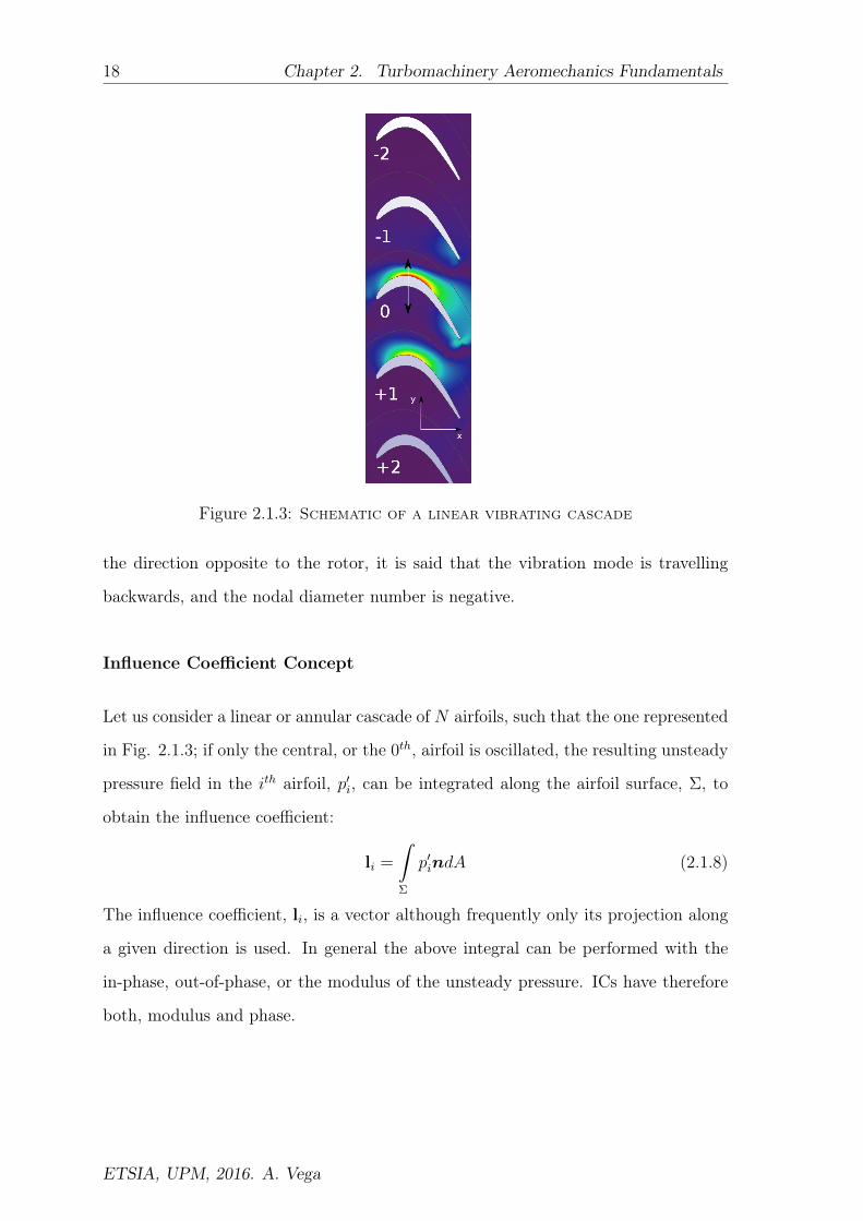
2.1.3 Schematic of a linear vibrating cascade . . . . . . . . . . . . . . 18
2.1.4 Frequency characteristics of the bladed-disc lumped model . 21
2.1.5 Sketch of the frequency correction (Left) and damping
(right) components of the quasi-stationary aerodynamic forces
as a function of the IBPA . . . . . . . . . . . . . . . . . . . . . . 23
2.3.1 Logarithmic decrement as a function of the normalised time . 35
3.2.1 Sketch of a slowly varying duct . . . . . . . . . . . . . . . . . . . 45
3.3.1 Generation of circulation by means of vortex shedding . . . . 51
ix

3.4.1 Control volume for a moving sphere . . . . . . . . . . . . . . . 55
3.5.1 Sketch of the Whitehead’s cascade . . . . . . . . . . . . . . . . . 58
3.5.2 Superresonant and subresonant regions as a function of the
IBPA for constant reduced frequency and Mach number, left
and right respectively. . . . . . . . . . . . . . . . . . . . . . . . . 59
3.6.1 Variation of phase angle between wall shear and oscillating
external velocity for a laminar flow over a flat plate
(∆V∞/V∞ = 15%) . . . . . . . . . . . . . . . . . . . . . . . . . . . . . 61
3.7.1 Moving surface of an oscillating airfoil . . . . . . . . . . . . . . 63
3.7.2 Non-dimensional work-per-Cycle as a function of the IBPA for
the flap and edge modes for k = 0.1 . . . . . . . . . . . . . . . . . 67
4.2.1 Typical hybrid-cell grid and associated dual mesh . . . . . . . 75
4.2.2 Close-up of the grid about an LPT airfoil. . . . . . . . . . . . 76
4.2.3 Schematic showing computational domain and boundary condi-
tions . . . . . . . . . . . . . . . . . . . . . . . . . . . . . . . . . . . 79
5.2.1 Position of the airfoil in an arbitrary time instant . . . . . . . 84
5.3.1 Non-dimensional damping as a function of the IBPA for the
LPT case vibrating in flap (M = 0.74, k = 0.1) for a viscous and
an inviscid case. . . . . . . . . . . . . . . . . . . . . . . . . . . . . . 94
5.3.2 Snapshot of the unsteady pressure caused by the vibration of
the central blade in an LPT airfoil for k = 0.3. . . . . . . . . . 96
5.3.3 Distribution of the normal gradient of the velocity
along an LPT airfoil computed using three different
approaches . . . . . . . . . . . . . . . . . . . . . . . . . . . . . . . 96
5.3.4 Unsteady loading parameter distribution (loading contribu-
tion, ULPL,and rotational contribution, ULPR) along an LPT
airfoil for different mode-shapes. . . . . . . . . . . . . . . . . . 97
x

5.3.5 Isentropic mach number distributions along the airfoil chord
for the LPT and the NACA65 cases . . . . . . . . . . . . . . . . . 98
5.3.6 Unsteady loading parameter distribution . . . . . . . . . . . 99
5.3.7 Unsteady loading parameter distribution for the NACA65
airfoil. (A): M1 = 0.7 . (B): M1 = 0.8. . . . . . . . . . . . . . . . . . 99
5.3.8 Imaginary part of the unsteady pressure of the NACA65
Compressor for k = 0.1, for Min = 0.7 (a) and for Min = 0.8
(b) . . . . . . . . . . . . . . . . . . . . . . . . . . . . . . . . . . . . . 101
5.4.1 Mean value and 1st harmonic of the non-dimensional work as a
function of the reduced frequency for the LPT case . . . . . 103
5.5.1 Sketch of the displacements of an isolated oscillating plate . 106
5.6.1 Sketch of the main conclusions . . . . . . . . . . . . . . . . . . . 110
6.0.1 Isentropic mach number distributions along the airfoil
chord (a) and sketch of the configurations (b) . . . . . . . 116
6.1.1 (a) Non-dimensional Influence Coefficient modulus and (b)
Phase as a function of the reduced frequency for the flat
plate case vibrating in flap (filled symbols) and torsion
around the l.e. (open symbols) . . . . . . . . . . . . . . . . . . . . 119
6.1.2 Non-dimensional damping as a function of the IBPA for an
asymmetric cascade of flat plates vibrating in flap mode
(filled symbols) and torsion about the plate midpoint (open
symbols) (M = 0.45, θ = 45, s/c = 0.5, k = 0.03) . . . . . . . . . . . . 120
6.1.3 Real (a) and imaginary (b) components of the unsteady
pressure for an asymmetric cascade of flat plates vibrating
in torsion about the l.e. (Min = 0.45, θ = 45, s/c = 0.5, k = 0.1) . . 122
6.1.4 (a) Real and (b) imaginary components of the unsteady
pressure for an asymmetric cascade of flat plates vibrating
in bending (Min = 0.45, θ = 45, s/c = 0.5, k = 0.1) . . . . . . . . . . . 122
xi
6.2.1 Isentropic Mach number distributions along the airfoil chord
for the LPT case for the design and off design conditions . . 124
6.2.2 (a) Non-dimensional Influence Coefficient modulus and (b)
Phase of the central airfoil as a function of the reduced
frequency for the LPT case vibrating in flap mode for the
different operating conditions . . . . . . . . . . . . . . . . . . . 125
6.2.3 Non-dimensional damping as a function of the IBPA and the
steady flow conditions for the low pressure turbine case
vibrating in flap (M = 0.74, k = 0.1) . . . . . . . . . . . . . . . . . 126
6.2.4 Isentropic Mach number distributions along the airfoil chord
for the NACA65 compressor for subsonic design and off design
conditions, and for design transonic conditions . . . . . . . . . 128
6.2.5 (a) Non-dimensional Influence Coefficient modulus and (b)
Phase as a function of the reduced frequency for the NACA65
case vibrating in flap mode for the i = 0ş (filled symbols) and
i = −3ş (open symbols) cases . . . . . . . . . . . . . . . . . . . . . 129
6.2.6 (a) Non-dimensional IC modulus of the 0th and ±1st airfoils as
a function of the reduced frequency and (b) non-dimensional
damping as a function of the IBPA and the reduced frequency
for the naca65 compressor (Min = 0.7) . . . . . . . . . . . . . . . 130
6.2.7 Phases of the 0th and ±1 airfoils as a function of the reduced
frequency for the naca65 compressor (Min = 0.7) . . . . . . . . . 130
6.2.8 (a) Non-dimensional Influence Coefficient modulus and (b)
Phase as a function of the reduced frequency for the NACA65
case vibrating in flap mode. M1 = 0.8: filled symbols and
M1 = 0.7: open symbols. . . . . . . . . . . . . . . . . . . . . . . . . . 132
6.2.9 Real (Left) and Imaginary (Right) part of the unsteady
pressure of the NACA65 Compressor for k = 0.1, for Min = 0.8
(a) and for Min = 0.7 (b) . . . . . . . . . . . . . . . . . . . . . . . . 133
xii

6.3.1 Non-dimensional work as a function of the IBPA for the LPT
case vibrating in flap, edge and different torsion modes (M =
0.74, k = 0.1) . . . . . . . . . . . . . . . . . . . . . . . . . . . . . . . . 135
6.3.2 (a) Non-dimensional IC modulus and (b) phase as a function
of the reduced frequency for the LPT case vibrating in flap
(filled symbols) and edge mode (open symbols). . . . . . . . . . 135
6.3.3 (a) Non-dimensional IC modulus and (b) phase as a function of
the reduced frequency for the NACA65 case vibrating in flap
(filled symbols) and edge mode (open symbols) . . . . . . . . . . 137
6.4.1 Mean (Filled symbols) and minimum (Open symbols) damping as
a function of the reduced frequency of the LPT and NACA65
(subsonic and transonic) configurations. . . . . . . . . . . . . . 138
6.5.1 Phase of the influence coefficients of the 0th and +1st
airfoils as a function of the Reduced frequency and Mach
numbers for a LPT airfoil. . . . . . . . . . . . . . . . . . . . . . . 140
6.5.2 Modulus of the force influence coefficients as a function of
the reduced frequency for M2 = 0.75 . . . . . . . . . . . . . . . . 141
6.5.3 Ratio between the modulus of influence coefficient 0 and +1
as a function of the Reduced frequency and Mach number . . 142
6.5.4 Variation of the influence coefficient of the central blade
with the square of the Mach number and the reduced frequency143
6.5.5 Non-dimensional work as a function of the IBPA and the Mach
number . . . . . . . . . . . . . . . . . . . . . . . . . . . . . . . . . . 145
6.5.6 Mean value and variation with the IBPA of the non-dimensional
work as a function of the mach number . . . . . . . . . . . . . . 145
6.5.7 Isentropic Mach number distribution normalized with the exit
Mach number for different exit Mach numbers. . . . . . . . . . 146
xiii

6.5.8 Effect of the reduced frequency and the M onto the work-
per-cycle curves . . . . . . . . . . . . . . . . . . . . . . . . . . . . 147
6.6.1 Snapshot of the unsteady pressure for the NACA0012 symmet-
ric case for k = 0.2 . . . . . . . . . . . . . . . . . . . . . . . . . . . 148
6.6.2 (a) Non-dimensional IC modulus and (b) phase of the 0th and
±1st airfoils as a function of the reduced frequency for the
NACA 0012 symmetric (filled symbols) and asymmetric (open
symbols) cases. . . . . . . . . . . . . . . . . . . . . . . . . . . . . . 149
6.6.3 Non-dimensional work as a function of the IBPA and the
reduced frequency for the NACA 0012 symmetric (a) and
asymmetric (b) cases. . . . . . . . . . . . . . . . . . . . . . . . . . . 150
6.6.4 Snapshot of the unsteady pressure for the NACA0012 asym-
metric case for k = 0.2 . . . . . . . . . . . . . . . . . . . . . . . . 151
6.7.1 Snapshot of the unsteady pressure cause by the vibration of
the central blade in a LPT airfoil for k = 0.3 . . . . . . . . . . 152
6.7.2 Isentropic Mach number and unsteady pressure modulus distri-
butions along blade surface for the: (a) 0th airfoil and (b)
+1st airfoil . . . . . . . . . . . . . . . . . . . . . . . . . . . . . . . 153
6.7.3 Phase distribution along the 0-th (left) and +1-th (right)
airfoils for different reduced frequencies. Solid line: Suction
side. Dashed line: Pressure side . . . . . . . . . . . . . . . . . . . 155
6.7.4 Mach number iso-contours and streamlines . . . . . . . . . . . . 156
6.7.5 Non-dimensional work as a function of the IBPA and the
reduced frequency for the edge mode . . . . . . . . . . . . . . . 157
6.7.6 Ratio between the modulus of influence coefficient -1,0 and
+1 as a function of the Reduced frequency and Mach number.
Fylled symbols: airfoil -1, empty symbols: airfoil 0 . . . . . . . 158
xiv

6.7.7 Mean value and 1st harmonic (variation with the IBPA) of the
non-dimensional work-per-cycle as a function of the reduced
frequency for the edge mode . . . . . . . . . . . . . . . . . . . . 158
6.7.8 Phases of the zeroth and 1 airfoils (filled symbols), and −1
airfoil (solid symbols) as a function of k and M . . . . . . . . . 159
6.7.9 Non-dimensional work as a function of the IBPA and the Mach
number for the edgewise mode. . . . . . . . . . . . . . . . . . . . 160
6.7.10Non-dimensional work as a function of the IBPA and the
reduced frequency for the torsion mode. . . . . . . . . . . . . 161
6.7.11Non-dimensional moment influence coefficients of the torsion
mode at two different reduced frequencies and M2 = 0.75. . . 162
6.7.12Modulus of the unsteady pressure distribution along the
airfoils of a linear cascade composed of nine airfoils (M2 =
0.75). . . . . . . . . . . . . . . . . . . . . . . . . . . . . . . . . . . . 163
6.7.13Phases of the influence coefficients of the torsion mode for
different Mach numbers. . . . . . . . . . . . . . . . . . . . . . . . 163
7.1.1 Layout of different bladed-disc assembly configurations . . . 168
7.1.2 1st flap mode-shape of a welded-in-pair rotor blade configur-
ation . . . . . . . . . . . . . . . . . . . . . . . . . . . . . . . . . . . 170
7.2.1 Schematic view of the non rotating annular test facility
(a) and turbine rotor cascade instrumentation, view from
downstream side (b) . . . . . . . . . . . . . . . . . . . . . . . . . . 171
7.2.2 Blade suspension system (left) and Probe traverse locations
(right) . . . . . . . . . . . . . . . . . . . . . . . . . . . . . . . . . . 173
7.3.1 Bending direction and torsion axis . . . . . . . . . . . . . . . . . 175
7.3.2 Isentropic Mach number distribution for different span heights 178
xv

7.3.3 Surface streamlines and isocontours of the unsteady pressure
modulus (flow moves from left to right) of the suction (Left)
and pressure (Right) sides for the bending mode and IBPA=90 179
7.3.4 Comparison of experimental and analytical results of the non-
dimensional work per cycle as a function of the IBPA for: (a)
bending mode and (b) torsion mode , for single blade (O), and
blade-pair (M) configurations, at k = 0.7 . . . . . . . . . . . . . . 179
7.3.5 Experimental (filled symbols) and numerical (opaque symbols)
unsteady pressure modulus distribution along the blade chord
for single blade and blade pair package configurations for
IBPA=-108ş and ISPA=-108, respectively at k = 0.7 for a bending
motion . . . . . . . . . . . . . . . . . . . . . . . . . . . . . . . . . . 180
7.3.6 Unsteady pressure modulus obtained from the simulations for
the torsion mode at k = 0.7. IBPA/ISPA=180ş. (a) single blade
configuration and (b) pair configuration . . . . . . . . . . . . . 181
7.4.1 Non-dimensional work per cycle as a function of the IBPA for
single blade and blade pair package configurations for: (a)
bending and (b) torsion mode, at k = 0.1. . . . . . . . . . . . . . . 183
xvi

List of Tables
5.1 Circulant and non-circulant contributions to the non-dimensional
lift lift . . . . . . . . . . . . . . . . . . . . . . . . . . . . . . . . . . 108
6.1 Unsteady loading parameter value for the LPT configur-
ation for different incidence angles . . . . . . . . . . . . . . 124
6.2 Unsteady loading parameter for the NACA65 configuration
for different incidence angles at M1=0.7 . . . . . . . . . . . . . 128
6.3 Unsteady loading parameter for the NACA65 configuration
for different inlet Mach number . . . . . . . . . . . . . . . . . . 131
6.4 Unsteady loading parameter for the LPT configuration for
the two fundamental bending directions and different torsion
centres . . . . . . . . . . . . . . . . . . . . . . . . . . . . . . . . . . 134
6.5 Unsteady loading parameter for the NACA65 configuration
for the two fundamental bending directions . . . . . . . . . . . 137
6.6 Unsteady loading parameter and slope of the φ − k curves
for the LPT and the NACA65 configurations for the two
fundamental bending directions . . . . . . . . . . . . . . . . . . . 138
6.7 Mach number effect in the phases of the influence coefficients
of the airfoils. V: Vortex shedding dominated. A: Acoustically
influenced. . . . . . . . . . . . . . . . . . . . . . . . . . . . . . . . . 166
7.1 upstream and downstream test conditions at 50% span . . . . . 176
xvii


Nomenclature
Latin symbols
a Sound speed
c Axial chord
cpp′
p0δc
f Blade excitation frequency (Hz)
F Convective fluxes
G,H Viscous fluxes
h Amplitude of blade translations
H Blade height
i Incidence
k =ωc
vcReduced frequency
kb Blade stiffness
kd Disc stiffness
K Stiffness matrix
l Influence coefficient modulus
Laero Matrix of aerodynamic forces
L Influence coefficients matrix
M Mach number
M Mass matrix
Md Disc mass
xix

mb Blade mass
n Nodal diameter
N Number of blades
pdyn Dynamic pressure
p′ Unsteady pressure
Re Reynolds number
s Pitch
S Blade surface
t Time
T Period of oscillation
U Vector of conservative variables
u, v, w Velocity components in cartesian coordinates
vc Characteristic velocity
V∞ Free stream velocity
W Non-dimensional velocity vector
W0 Non-dimensional mean velocity
w(x, τ) Non-dimensional perturbed velocity
Wcycle Work-per-cycle per span unit
x Chordwise direction
Greek Symbols
α Torsion amplitude (rad)
α1,2 Inlet/outlet flow angles
∇W0 Velocity gradient in the wall normal direction
δ Vector of the airfoil vibration amplitude
µ Mass ratio
xx

µd = Md/mb Disc to rotor blade mass ratio
κ = kdisc/kblade Disc to blade stiffness ratio
ρa Characteristic density of the air
σ Inter-blade phase angle
Σ Computational domain boundary
τ = ωt Non-dimensional time
τξη Viscous shear stresses
Ω Control volume
Υ Unsteady loading parameter
Γ Vorticity
ξ x-direction
η y,z-directions
ω Oscillation frequency (rad/s)
Abbreviations
ADP Aerodynamic Design Point
EO Engine order
HEO High engine order
h.o.t Higher-order terms
HPT High pressure turbine
IBPA Inter blade phase angle
IC Influence coefficient
ISPA Inter sector phase angle
l.e. Leading edge
LEO Low engine order
LPT Low Pressure Turbine
xxi
NSV Non-synchronous vibration
PS Pressure side
RANS Reynolds averaged Navier Stokes
SS Suction side
r.h.s Rigth hand side
t.e Trailing edge
TW Traveling wave
ULP Unsteady loading parameter
URANS Unsteady Reynolds averaged Navier Stokes
Subscripts
c Characteristic
cyc Per-cycle
in Inlet
I Imaginary part of a complex number
is Isentropic
0 Base flow
out Outlet
t Total
R Real part of a complex number
Superscripts
’ Unsteady value
ˆ Complex number
˜ Non-dimensional value
xxii

Chapter 1
Introduction
Start by doing what’s necessary;
then do what’s possible; and
suddenly you are doing the
impossible
Francis of Assisi
Contents
1.1 Context . . . . . . . . . . . . . . . . . . . . . . . . . . . . . 1
1.2 Motivation . . . . . . . . . . . . . . . . . . . . . . . . . . . 2
1.3 Turbomachinery Aeroelasticity Background . . . . . . . . 4
1.1 Context
The unsteady pressure field caused by airfoil vibration plays a major role in the
flutter and forced response of turbomachinery blade rows. Flutter is a self excited
aeromechanic instability by which energy is extracted from the main stream and
transferred to the structure. When the energy dissipated by the structure is smaller
than that taken out from the flow, the vibration amplitude grows, leading eventually
1
2 Chapter 1. Introduction
to either an instantaneous or a high cycle fatigue (HCF) failure of the structure,
depending on the mechanical damping level. On the other hand, blades and vanes
undergo periodic excitations due to the relative motion of neighboring blades. The
vibration caused by these excitations may also provoke an HCF failure if the resulting
vibration amplitude is large enough. It is well known that the largest response of the
structure takes place at resonant conditions, when the frequency of the excitation
matches one of the natural frequencies of the system. Under these conditions the
vibration amplitude is directly proportional to the excitation force and inversely
proportional to the overall damping, of which a significant part may be due to the air
stream in which the airfoil is immersed. In both phenomena, the unsteady pressure
field induced by the airfoil oscillation and its subsequent interaction with the structure
are essential in determining the aerodynamic damping and, therefore, the life of the
component.
1.2 Motivation
Aerodynamics of oscillating airfoils is equally important for both flutter and forced
response. However the range of reduced frequencies, k, i.e.:, the ratio between the
flow-through or residence time of the fluid, tr = c/vc, and the inverse the angular
frequency of the vibration, ω, may be quite different. Whereas flutter typically occurs
at the lowest modes of the assembly, forced response is usually of interest at higher
modes, since resonant crossings with the first modes are avoided whenever possible
by design; an exception of this case being the analysis of crossings at large off-design
conditions. As a consequence, the reduced frequency of a flutter analysis is, generally
speaking, much lower than that of a forced response study.
Flutter primarily affects high-aspect ratio rotor blades found in the fan, fore high-
pressure compressor stages, and aft low-pressure turbine stages, because low natural
frequencies and high axial velocities give rise to low reduced frequencies. Aeronautical
low-pressure turbines (LPTs) are made of very slender and thin airfoils because
their weight and cost have a large impact on the engine (about 20% of the total
ETSIA, UPM, 2016. A. Vega

1.2. Motivation 3
weight and 15% of the total cost). Natural frequencies of LPT rotor blades are
very low exhibiting very low reduced frequencies as well (k ∼ 0.1 − 0.2) and, as a
consequence, LPT bladed-discs are prone to flutter. Nowadays flutter may become a
dominant constraint on the design of modern LPTs precluding the use of more efficient
aerodynamic configurations [1, 2]. Compressor airfoils have a much lower aspect ratio
than that of the LPTs, and usually the reduced frequency of their lowest modes is of
order unity (k ∼ 1.0). However, it is still interesting to study their behavior in the
k 1 limit, as a means to increase the overall understanding of vibrating airfoils at
low frequency, and in particular the sensitivity to the airfoil shape.
The unsteady aerodynamics associated with the vibration of turbine and compressor
bladed-discs and stator vanes is nowadays routinely analyzed within the design loop
of the aeroengine companies, and it has been the subject of dedicated experiments in
the past [3, 4, 5]. The aim of these simulations is the derivation of the aerodynamic
stability of the rotor blades and the quantification of the aerodynamic damping, which
is the result of the application of the unsteady pressures on the airfoil displacements.
With a few exceptions in the early days of aeromechanics [6, 7], little attention
has been paid to the understanding of vibrating airfoil aerodynamics since this is
not a figure of merit in itself for the aeroelastic analyst. Designers obtain and use
aerodynamic data from efficient numerical tools, but they do not usually examine
critically the resulting unsteady flow-field, since they are really just interested in
the global aerodynamic damping. As a direct consequence of using aerodynamic
codes as black boxes, little understanding has been gained in recent years about
the physics of these type of flows and its impact on the aerodynamic damping.
Although there are several trends that are well known, such as the stabilization with
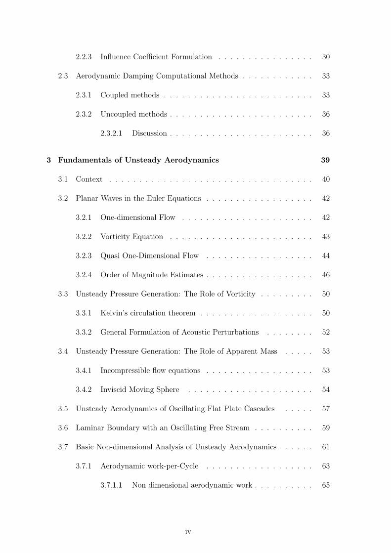
the reduced frequency (see Fig. 1.2.1), the physics which is behind this behavior is
not really well understood and the statement lacks of a sound theoretical support.
Another example is the shape of the damping curves as a function of the inter-blade
phase angle (IBPA) of LPTs and compressors, that look quite different without a
clear rational of which is the underlying reason for this (see Fig. 1.2.1). On the
other hand, vibrating cascade experiments are scarce, and performed well apart in
ETSIA, UPM, 2016. A. Vega

4 Chapter 1. Introduction
−180 −135 −90 −45 0 45 90 135 180
IBPA
−2
−1
0
1
2
3
4
Θ=
Wcycle/(
πρ
cU
c
2δ
2
c/2
)
Unstable
Stable
k
−180 −135 −90 −45 0 45 90 135 180
IBPA
−1
0
1
2
3
4
Θ=
Wcycle/(
πρ
cU
c
2δ
2
c/2
)
Unstable
Stable
k
(a) (b)
Figure 1.2.1: Non dimensional work per cycle curve trends as a function ofthe reduced frequency for an LPT (a) and the NACA65 configuration (b)
time in different institutions [8, 9, 10, 11, 12] with different techniques, parameter
range, etc., and therefore, are not well suited for conceptual and systematic studies.
The main objective of this thesis is hence to study the unsteady aerodynamics of
oscillating airfoils in the low reduced frequency regime, with special emphasis on
finding a theoretical support which allows us to predict the behaviour of the work-
per-cycle curves, understand the physics of the problem and predict the work-per-
cycle trends as a function of different physical parameters, even before carrying out
the actual numerical simulations. However, although the topic is strongly related
with turbomachinery flutter, and many conclusions can be directly drawn from the
results, this thesis is not believed to address the whole flutter problem, since relevant
mechanical issues such as mistuning and friction are not treated at all in this work.
1.3 Turbomachinery Aeroelasticity Background
1.3.1 Definition
Aeroelastic problems has been around since the early days of turbomachinery design
and they have been object of study for many years.
The science that studies physical phenomena related with the interaction between
aerodynamic, elastic and inertial forces is called aeroelasticity, and it is of a highly
interdisciplinary character. Collar’s triangle (see [13]), shown in Fig. 1.3.1, and which
ETSIA, UPM, 2016. A. Vega

1.3. Turbomachinery Aeroelasticity Background 5
Elastic
Forces
Inertial
Forces
Aerodynamic
Forces
Sta
bility
and C
ontro
l
Vibration
Sta
tic
Aero
ela
stic
ity
Dynamic
Aeroelasticity
Figure 1.3.1: Collar’s triangle of forces
is formed by putting in each of its vertex the forces contributing to the aeroelastic
problem, illustrates this interrelation. From this triangle, it can be shown the different
types of problems studied in aeroelasticy as a function of the most relevant forces
in that problem. The interactions among the three types of forces, located in the
vertexes of the triangle in Figure 1.3.1, give rise to four disciplines: classical vibration,
which is concerned with the interaction of inertial and elastic forces, stability and
control, which are affected by the interaction of aerodynamic and inertial forces, static
aeroelasticity, which describes the interaction of aerodynamic and elastic forces and
finally dynamic aeroelasticity, which is the discipline which deals with the interaction
of all the three forces. In turbomachinery both static and dynamic aeroelasticity are
a major cause of concern since blade rows are subjected to high centrifugal loads and
unsteady aerodynamic forces.
1.3.2 Static Aeroelasticity
Static aeroelasticity describes the interaction of aerodynamic and elastic forces. It is
therefore a vibration-free phenomenon and refers to the deformation of a structure
under steady aerodynamic loads. Turbomachinery blade-rows are subject to large
variations of rotational speeds and flow conditions (aircraft engines must endure
take off, acceleration, cruise, descent, and landing conditions during their flight
ETSIA, UPM, 2016. A. Vega
6 Chapter 1. Introduction
envelope). Flow conditions and rotational speed dictate the gas and centrifugal
loads. As the centrifugal loads change, so does the stiffness of the blades, which
deform elastically from their initial manufactured (or cold) shapes to their running
shapes. This deformation can be significant and its prediction crucial to stability.
Static turbomachinery aeroelasticity is related to the study of such deformations. The
determination of the final shape of the rotor blade can be of paramount important
for fans operating at transonic conditions, where minor modifications in the final
position of the blade can lead to significant variations in its aerodynamics.
1.3.3 Dynamic Aeroelasticity
Dynamic aeroelasticity is the study of problems caused by the interaction of unsteady
fluids with blade vibration. The main aeroelastic phenomena of interest are: forced
response, flutter and non-synchronous vibrations (NSV). Both, flutter and force
response are a potential source of blade failure in turbomachines and, sometimes,
it is difficult to distinguish between them and to know the exact reason for failure .
1.3.4 Forced Response
Forced response is a synchronous problem which occurs when the frequency of an
unsteady aerodynamic load, that is the result of the rotor’s motion through a non-
uniform flow, coincides with one of the bladed-disc natural frequencies. The excitation
frequency is a multiple of the a so-called engine order, EO, i.e.: f = EO Ω. It
can be distinguished between two types of forced response: classical forced response
(high engine order), which is caused by the rotation of a rotor through the wake or
potential field of an upstream or downstream stator, and low engine order (LEO)
forced response caused by the rotation through a long wave-length non-uniformity
(much greater than the pitch of the stator vanes) created, for example, by gusts,
aerodynamically mistuned assemblies or staggered blades. The characterization of
this type of forcing remains still today as a major challenge [14].
ETSIA, UPM, 2016. A. Vega

1.3. Turbomachinery Aeroelasticity Background 7
3EO
4EO
2EO
1EO
2F
1T
1F
Shaft Speed
Fre
quen
cy
Figure 1.3.2: Schematic of a Campbell diagram
Campbell’s diagram (Fig. 1.3.2) represents the bladed rotor eigenfrequencies versus
the rotational speed and it is an useful and widely used aeroelastic tool to predict
potential forced response mechanisms, at the crossings of the excitation sources (EO)
with the natural frequencies. In the same figure, the points corresponding to flutter
are marked up in blue. The latter phenomenon is described in the following lines.
1.3.5 Flutter
Flutter is a ‘sustained oscillation due to the interaction between aerodynamic forces,
elastic response and inertia forces’ [15], but unlike forced response, flutter is a self
excited vibration, and it does not require the presence of any unsteadiness coming
from the interaction with upstream or downstream rows. Technically speaking flutter
is an aero-mechanic dynamic instability. As flutter occurrences are not bound to
engine order lines, and therefore can occur at any rotational speed, the predictive
assessment of flutter can not be done recurring to the Campbell’s diagram.
The vibration occurs at the natural modes and frequencies of the whole aeroelastic
problem, but the aerodynamic forces resulting from the oscillations could be large
enough to alter the vibration characteristics of the purely structural problem. The
perturbation of the non-dimensional frequency being of the order of the critical
damping ratio, if several modes are closely spaced in frequency, the aerodynamics
can significantly modify the mode-shapes, and the structure exhibits flutter in a
ETSIA, UPM, 2016. A. Vega
8 Chapter 1. Introduction
Tmp
Choke Flutter
Transonic Stall Flutter
Subsonic Stall Flutter
Supersonic Stall Flutter
Supersonic Unstall Flutter
25%
75%
50%
100%
Choke Line
π
Surge LineOperating Line
Figure 1.3.3: Classical compressor flutter map
coupled mode (which is different, in mode-shape and frequency, from the original
natural modes). The extent to which purely structural natural modes are affected
by aerodynamic forces depends on its mass ratio (the ratio of the mass of the
rotor blade to the mass of the surrounding fluid). Wings, for example, are light
weight structures which typically flutter in a coupled bending-torsion mode whereas
traditional turbomachinery blades predominantly flutter in a single mode shape close
to their in-vacuo frequency. However, coalescence (coupled bending-torsion) flutter
has also been observed on modern low mass ratio, low solidity fans [16], and turbine
sectored vanes. [17].
A few major differences separate aeroelastic phenomena on turbomachinery-blades
from the ones for an aircraft wing: the construction of the rotor blade, the
cyclic symmetry of the structure, and the aerodynamic coupling effects between
neighbouring blades. Wing flutter is driven by a ‘mode coalescence’ phenomena
whereas turbomachine flutter is mostly driven by the blade-to-blade coupling.
Neighboring blades can perform vibrations with a certain inter-blade phase difference,
which considerably influences the time-dependent aerodynamic response. Another
main difference is that the coupling between aerodynamics and structural dynamics
in turbomachinery flutter problems is relatively weak compared to the aeroelasticity
of isolated wings.
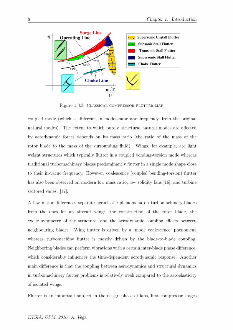
Flutter is an important subject in the design phase of fans, first compressor stages
ETSIA, UPM, 2016. A. Vega

1.3. Turbomachinery Aeroelasticity Background 9
Figure 1.3.4: Phase lag between blade motion and aerodynamic forces
and aft turbines stages, where the blades are slender. Four main categories of flutter
are encountered in turbomachinery, namely: classical flutter, stall flutter, acoustic
flutter, and choke flutter. Figure 1.3.3 represents a sketch of a compressor map and
the regions where different types of flutter may occur. Flutter in turbines is only of
concern at Maximum Take-Off (MTO) and a similar sketch does not exist.
Classical Flutter
Flutter is named classical when the flow remains attached to the blade with no
separation along the whole vibration cycle, and the phenomenon is essentially inviscid.
Flutter instability is due to the phase between the aerodynamic forces acting on the
airfoil and the airfoil displacements. Depending on whether the force is lagging or
leading the displacement the flow feeds in or absorbs energy from the blade, and the
motion is amplified or damped respectively. This fact is sketched if Fig. 1.3.4. It can
be said that flutter is all about phasing, the only difference among the different types
is the origin of the phasing. In classical flutter the lag between the blade motion
and the pressure is due to vortical and acoustic waves, and the interaction with the
neighbouring airfoils. This type of flutter is the one which is closely with the subject
of this thesis.
ETSIA, UPM, 2016. A. Vega

10 Chapter 1. Introduction
Stall Flutter
Stall flutter is an aeroelastic instability affecting the blades of fans and compressors
that occurs near the stall line. Typically, stall flutter occurs at part speed, and at
high mean flow incidence angles and/or low reduced frequencies. As the mass flow
decreases and the pressure ratio increases (near the stall boundary), the incidence of
the blade increases and the flow eventually stalls. For stall flutter, flow separation
is the key driver because: i) it creates significant unsteadiness behind the shock and
ii) it changes the phase of the unsteady pressure so that it is out-of–phase with the
blade motion. Frequently, the mode of blade vibration, in large fans, is the first
bending mode, but flutter may occur in torsion as well; though other compressor
and low-pressure turbine blades may also suffer from such instabilities. In the main,
flutter is observed in one to six forward traveling nodal diameter assembly modes
[18]. Usually stall flutter correlations express maximum incidence as a function of
the reduced frequency [19], but these correlations heavily rely on a specific type of
blade and base flow [20, 21, 22].
Near design speed, a fan operating at supersonic tip Mach numbers can exhibit
supersonic stalled flutter at high pressure ratios. It is believed that this type of
flutter is caused by movement of a strong passage shock and boundary layer separation
[23]. On the other hand, near design speed, a fan operating at supersonic tip Mach
numbers at low pressure ratios can exhibit supersonic unstalled flutter. In this case,
the phenomenon is caused by the motion of a impinging shock originating from the
neighbouring blade and is therefore associated with an inter-blade phase angle [24].
Acoustic Flutter
Acoustic flutter is encountered when acoustic waves, generated by the blade vibration,
are reflected back onto the vibrating blade and feed the vibration. For this to happen,
the temporal frequency of the acoustic wave must be equal to one of the natural
frequencies of the blade, and must correspond to a resonant (or cut-on) mode of
the annulus. For example, some acoustic flutter are known to occur due to the
ETSIA, UPM, 2016. A. Vega

1.3. Turbomachinery Aeroelasticity Background 11
interaction between the fan blades and the engine intake. Acoustic flutter may occur
on its own since the wave reflection mechanism is independent of flow separation.
However, acoustic flutter is unlikely to be a problem on its own since blade-only
damping is usually quite high when there is no flow separation and there will also
be some inherent mechanical damping in the system. Nevertheless, acoustic flutter
can exacerbate the stall flutter very significantly. It is important to say that the use
of blade frequency, say increase the reduced frequency by stiffening the blade, for
stability control will not necessarily alleviate the acoustic flutter, since damping is
not a monotonically increasing function of blade frequency [25, 18].
This type of flutter can occur even when the slope of the pressure rise characteristic
is still negative, since stall is not the driven mechanism, and is referred to as “flutter-
bite” sometimes. It happens in low nodal diameter forward cut-on traveling waves,
frequently in first flap (1F) mode of blade vibration.
Choke Flutter
Compressors operate in a wide range of pressure ratios and shaft speeds, that give rise
to quite different base flow-fields. A particular case is that in which there is a shock
wave inside the compressor passage (see Fig. 1.3.5). The shock-wave extends from
the trailing-edge of the suction side to the pressure side. In this case, the instability
is caused by the shock wave oscillation between neighbouring airfoils caused by the
airfoil vibration that modifies the throat area. The instability occurs at large reduced
frequencies (k= 0.3−0.4) and the sensitivity to this parameter is low. Choke flutter
is less common than other types of compressor flutter and it is usually experienced
by middle and rear compressor stages. The numerical prediction of the instability is
difficult (see [26]) since this is the result of the compensation of two large quantities:
the oscillation of the shock-wave causes large unsteady perturbations in its vicinity,
both in the pressure and suction sides. The pressure side is stabilizing while the
suction side is destabilizing. The global result depends on the subtraction of both
quantities.
ETSIA, UPM, 2016. A. Vega

12 Chapter 1. Introduction
Figure 1.3.5: Mach number contour plot of a choked compressor airfoil
The problem is highly non-linear, since the perturbations caused by the oscillation
of the shock-wave are large. In this case, it has been shown that the stability of the
system depends on the vibration amplitude. For small amplitudes the system may
be unstable, but for large vibration amplitudes the non-linearity may lead to a stable
situation [26].
1.3.6 Non-synchronous Vibrations (NSV)
Non-Synchronous Vibration (NSV), is the interaction of an aerodynamic instability
(like leading-edge vortex shedding or rotating stall) with natural turbomachinery
blade vibrations. NSV can occur in the fan, compressor, and turbine stages of the
turbomachine, though it is most often found in compressors. NSV has been shown to
be very sensitive to parameters like tip clearance shape and size, and back-pressure
[27]. It also occurs at many different pressure ratios and mass flow conditions, and at
non-integral multiples of the shaft rotational frequencies, [28]. The blade vibrations
due to NSV are generally frequency and phase locked. Hence, NSV occurs at one
dominant frequency and one inter-blade phase angle.
ETSIA, UPM, 2016. A. Vega
Chapter 2
Turbomachinery Aeromechanics
Fundamentals
Everything should be made as
simple as possible, but not simpler
Albert Einstein
Contents
2.1 Simplified Aeroelastic Model . . . . . . . . . . . . . . . . . 13
2.2 Formulation of the Tuned Flutter Problem . . . . . . . . 24
2.3 Aerodynamic Damping Computational Methods . . . . . 33
2.1 Simplified Aeroelastic Model
Nowadays, linear bladed-disc dynamics is computed routinely by gas turbine
manufacturers using finite element methods. Complex blade shapes and discs are
discretised using automatic grid generators, the governing equations are written in
discrete form, and the eigenvalue problem of the resulting set of ordinary differential
equations is solved, to obtain the natural frequencies and mode-shapes of the
assembly.
13

14 Chapter 2. Turbomachinery Aeromechanics Fundamentals
0 MaxNDNodal Diameter
Norm
alizedfrequency
ND=3
t Family
2nd Family
3rd Family
Disk Mode
Blade Alone
Figure 2.1.1: Sketch of the natural frequencies of a bladed-disc as afunction of the nodal diameter
Rotor blades are coupled with their neighbours via the structural connections that
inevitably exists either through the discs, the casings in the case of stator vanes, or
through the shroud rings, that are included to stiffen the assembly. The structural
coupling among different rotor blades significantly influences the natural frequencies
and mode-shapes of the assembly, and need to be retained in the simulations. Analysis
including just a single rotor blade must be regarded as a first step in the simulation
process. Perfectly tuned bladed-discs exhibit cyclic symmetry, and then the whole
wheel may be splitted in N identical sectors, also containing several airfoils, as it
is always the case for sectored vanes, and impose cyclic boundary conditions in the
periodic boundaries to reduce the computational domain. Solving a single sector
using cyclic symmetry boundary conditions considerably reduces the computational
time required to solve the problem.
Discs, or any continuous structure with cyclic-symmetry vibrate in double nodal
diameters. Mode-shapes with more nodal diameters have higher natural frequencies
since the mode is stiffer. As the excitation frequency increases the disc may exhibit
nodal circles which are points at constant radius with zero displacement.
Bladed-Discs are constructed fixing rotor blades to a disc, either using fir-tree or dove
tail attachments, or welding the rotor blades to the disc, or even machining integral
ETSIA, UPM, 2016. A. Vega

2.1. Simplified Aeroelastic Model 15
parts with discs and blades, as it is usually the case in small compressors and fans
(blisks).
Figure 2.1.1 displays the frequency versus the nodal diameter of a generic bladed-
disc. Horizontal lines represents the frequency that would be obtained by clamping
the rotor blade at the attachment, that does not depend on the nodal diameter, since
the disc is not included in the representation. The parabola-like curve represents the
natural frequencies of disc dominated modes, that steeply increase with the nodal
diameter.
A very short review of the underlying concepts of bladed-disc dynamics resorting to
a simplified lumped model that contains all the key ingredients is presented in the
next sub-sections. Aerodynamic forces are also included in the mass-springs model,
to show their impact on the solution and the differences with the purely mechanical
problem. These are essential to explain the basic concepts and characteristics of the
aeroelastic problem.
2.1.1 Bladed-Disc Lumped Model
A tuned bladed-disc formed by a disc and a set of rotor blades attached to it can be
represented from a conceptual point of view (see Fig. 2.1.2) as a ring on N identical
masses,Md, joined by a spring of stiffness kd, that represents the disc, and N identical
masses, mb, that represent the rotor blades, linked to the corresponding disc sector
through a spring of stiffness kb. The aerodynamic forces can be written in terms of
the influence coefficients as:
faeroj =i=1∑i=−1
(liyj+i + l∗i
dyj+idt
)(2.1.1)
where li is the force influence coefficient of the blade ith acting on the blade 0th.
Here only the effect of the immediately neighbouring airfoils has taken into account
for the sake of simplicity, but this fact does not qualitatively change the problem.
Actually, this is the most typical situation. The influence coefficients will be defined
and properly explained later on, at this point they are just introduced in order to
ETSIA, UPM, 2016. A. Vega

16 Chapter 2. Turbomachinery Aeromechanics Fundamentals
Figure 2.1.2: Simplest lumped model of a bladed-disc
formulate the aeroelastic problem.
If only the 0th term of the above expression is included, the force is always in phase
with the displacement and there is no damping. In general, a second term, that
accounts for the effect of the velocity, l∗i , is included to better represent the physics
of the problem at high frequencies. It is important to highlight that this is a linear
model of the aerodynamic forces, since these are always proportional to the amplitude
of the displacements of the neighbouring blades. The discussion of the validity of this
approach is postponed to the next chapters, so far it is enough to know that li and
l∗i are given constant coefficients. The governing equations of the simplified bladed-
disc, including the aerodynamic contribution, which in turn constitute the simplest
aeroelastic problem, are then:
Mdd2xjdt2
= +kblade(yj − xj) + kdisc(xj+1 − xj)− kdisc(xj − xj−1)
mbd2yjdt2
= −kblade(yj − xj) +i=+1∑i=−1
(liyj+i + l∗i
dyj+idt
) (2.1.2)
That in non-dimensional form becomes:
µdd2xjdτ 2
= +(yj − xj) + κ(xj+1 − 2xj + xj−1)
d2yjdτ 2
= −(yj − xj) +i=+1∑i=−1
(liyj+i + l∗i
dyj+idτ
) (2.1.3)
where µd = Md/mb is the disc to rotor blade mass ratio, κ = kdisc/kblade is the disc
to blade stiffness ratio, li = limbω
2band l∗i =
l∗imbωb
are the non-dimensional influence
coefficients, and τ = ωbt the non-dimensional time, where ω2b = kblade/mb is the
natural frequency of the mass representing the rotor blade clamped to a infinitely
stiff disc.
ETSIA, UPM, 2016. A. Vega

2.1. Simplified Aeroelastic Model 17
Looking for solutions in travelling-wave form:
xj = xei(nθj+ωτ), yj = yei(nθj+ωτ) (2.1.4)
where θj = j 2πN
and n = 0, ...,±N/2 if N is even. The non-dimensional angular
frequency, ω, is defined as ω = ω/ωb. Introducing the previous expressions in the
governing equations, the following eigenvalue problem is obtained: 1− µdω2 + 4κ sin2 σ2
−1
−1 1− ω2 − faero
x
y
=
0
0
(2.1.5)
where
σ = 2πn
N(2.1.6)
represents the temporal phase lag between the motion of an airfoil and its neighbour,
which is usually referred to as the inter-blade phase angle (IBPA), and the non-
dimensional aerodynamic force coefficient, faero, is :
faero = l0 + i ωl∗0 +(∆l+ + iω∆l∗+
)cosσ + i
(∆l + iω∆l∗−
)sinσ (2.1.7)
where ∆l+ = l+1 + l−1, ∆l− = l+1 − l−1, ∆l∗+ = l∗+1 + l∗−1 and ∆l− = l∗+1 − l∗−1.
Inter-Blade Phase Angle Concept
The IBPA is defined as the temporal shift between the motion of a blade and the
motion of its neighbour, and is one of the most fundamental concepts in aeroelasticity
of turbomachines. Assuming that all the airfoils from the cascade are identical,
separated by the same pitch, vibrating with the same common angular frequency,
with a constant phase shift between adjacent blades (i.e.: in travelling-wave form),
the IBPA can be written as a function of the number of diameters at which the airfoils
have zero displacement, n, (also called nodal diameters) and the number of blades in
the current blade-row, N , as σ = 2πn/N.
In the case of a rotor blade, when the vibration is propagating in the same direction
as the rotor, it is said that the vibration is travelling forward, and the nodal diameter
number is positive. On the other hand, when the vibration mode is rotating in
ETSIA, UPM, 2016. A. Vega
18 Chapter 2. Turbomachinery Aeromechanics Fundamentals
Figure 2.1.3: Schematic of a linear vibrating cascade
the direction opposite to the rotor, it is said that the vibration mode is travelling
backwards, and the nodal diameter number is negative.
Influence Coefficient Concept
Let us consider a linear or annular cascade of N airfoils, such that the one represented
in Fig. 2.1.3; if only the central, or the 0th, airfoil is oscillated, the resulting unsteady
pressure field in the ith airfoil, p′i, can be integrated along the airfoil surface, Σ, to
obtain the influence coefficient:
li =
ˆ
Σ
p′indA (2.1.8)
The influence coefficient, li, is a vector although frequently only its projection along
a given direction is used. In general the above integral can be performed with the
in-phase, out-of-phase, or the modulus of the unsteady pressure. ICs have therefore
both, modulus and phase.
ETSIA, UPM, 2016. A. Vega

2.1. Simplified Aeroelastic Model 19
2.1.2 Purely structural problem
If faero = 0, the characteristic equation reduces to:
µdω4 −
[(µd + 1) + 4κ sin2 σ
2
]ω2 + 4κ sin2 σ
2= 0 (2.1.9)
and then, the natural frequencies of the problem depend on three parameters:
ω2 =ω2n
ω2blade
= F(µd =
Mdisk
mblade
, κ =kdisckblade
, σ = 2πn
N
)(2.1.10)
the disc to rotor blade mass ratio, µd, the disc to rotor blade mass stiffness, κ, and
the non-dimensional wave number, nodal diameter, or IBPA, σ, depending on the
nomenclature the reader is more familiar with.
There are a number of conclusions that may be drawn from the mathematical
structure of the problem that have their physical counter part:
1. All the eigenvalues, ω2, of the model problem are real. This may be readily
seen by noting that the characteristic equation 2.1.9 is a second order equation
of the form ω4 − 2bω2 + c = 0, whose solution is ω2 = b±√b2 − c. Since b and
c are always positive , and b2 > c, then ω2 is always real and greater than zero.
This physically means that the system is not damped and it is conservative,
since the solution can be expanded in a series of sines and cosines of constant
amplitude according to 2.1.4. A more general view of the problem can be
obtained by noting that the matrix of the eigenvalue problem is symmetric,
and hence all its eigenvalues are real. In general, the matrices resulting from a
purely structural eigenvalue problem with cyclic symmetry boundary conditions
are Hermitian, and therefore all the eigenvalues are again real.
2. The eigenvalues are double, since Eq. 2.1.4 does not change for positive or
negative nodal diameters or wave numbers, n, i.e ω2(σ) = ω2(−σ). This means
that from a purely structural point of view the system is symmetric and then
eigenfunctions with the same eigenvalue can be arbitrary combined between
them. This directly implies that the solution of the purely structural problem
can be expressed in the form of either traveling waves (TW) or standing waves
ETSIA, UPM, 2016. A. Vega

20 Chapter 2. Turbomachinery Aeromechanics Fundamentals
(SW). The angular wave-length of the waves is λθ = 2π/n. It can be anticipated
that this symmetry of the structural problem is spoiled when the aerodynamic
forces are introduced.
3. From a mathematical point of view the natural form of looking at the solution
is as pairs of forward and backward travelling waves of wave-length λ and phase
velocity c = ±ω/n
x(t) = An cos(nθ + ωτ) +Bn cos(nθ − ωτ + φ) (2.1.11)
however this solution may be recombined and expressed as two standing-waves,
setting φ = 0:
x(t) = (An +Bn) cos(nθ) cos(ωτ)− (An −Bn) sin(nθ) sin(ωτ) (2.1.12)
Frequently rotor blade and disc masses are comparable, µd ∼ 0(1). This is true for
low-pressure turbines and compressors whereas high-pressure turbines tend to have
much heavier discs, due to the combined effect of high shaft rotational speeds and
high temperatures. Following the same line, compressor blisks tend to have very light
blades. The disc is dynamically very stiff in the high nodal diameter limit if κ µd;
more strictly when, i.e.: 4 κµd
sin2 σ2
= 1ε 1,. The dispersion relation reduces in this
case to:
εω4 − ω2 + 1 = 0 (2.1.13)
and hence ω2Disk = 1
εand ω2
Blade = 1. This means that the natural frequencies of the
rotor blade dominated modes are quite similar to that of the blade alone case (see
Fig. 2.1.4). There is always a region, for low enough nodal diameters (σ ∼√µd/κ),
in which the flexibility of the disc can be noticed. For very stiff discs this region
is fairly small and a good approximation to characterise the damping is to consider
mode families of constant frequency. This approach has been systematically followed
in this thesis.
ETSIA, UPM, 2016. A. Vega

2.1. Simplified Aeroelastic Model 21
1+µ
µ
n
N
κ
µsin
πn
N
2
κ
1+ µ
2πn
N
κ−1/2
1
1
Blade
Disc
ω
Figure 2.1.4: Frequency characteristics of the bladed-disc lumped model
2.1.3 Aerodynamic contribution
When the aerodynamic forces are retained (faero 6= 0), the new characteristic equation
is:
µdω4−[(µd + 1) + 4κ sin2 σ
2− µdfaero
]ω2 + 4κ sin2 σ
2(1− faero)− faero = 0 (2.1.14)
It is important to express the aerodynamic forces (Eq. 2.1.1) as a function of a
physical scaling and in non-dimensional form, to better understand the functional
dependence of the whole problem.
faeroj =faeroj
mbω2b
=i=1∑i=−1
(1
µk2li(k)yj+i +
1
µkl∗i (k)
dyj+idτ
)(2.1.15)
where the mass ratio, µ, is defined as µ = mb/Hρac2
, and the reduced frequency as
k = ω0c/vc, being H the airfoil span, ρa, the characteristic density of the air, c
the airfoil chord, and vc the characteristic velocity. Since mb/H ∼ ρsc t, where t is
the characteristic thickness of the airfoil, and ρb the density of the rotor blade, the
order of magnitude of the mass ratio for a solid rotor blade is µ ∼ (ρb/ρa)(t/c). The
density ratio can range between 103to 104, whereas the relative thickness is around
10−1, therefore the density ratio for a solid blade is close to 103. Then, even if the
reduced frequency is very low, k ∼ 10−1, fjaero 1 and is only a small, but relevant,
correction to the structural part.
Equation 2.1.15 has been derived assuming that the force per unit deflection due to
the quasi-static displacement of the airfoils is proportional to the dynamic head and
ETSIA, UPM, 2016. A. Vega
22 Chapter 2. Turbomachinery Aeromechanics Fundamentals
the airfoil span, li ∝ ρaU2cH, and the force per unit velocity is l∗i ∝ ρaUccH. The
scaling rational will be specifically addressed in other chapters. It is worth noting
that the new aerodynamic based non-dimensional form of the influence coefficients is
li = liρav2cH
and l∗i =l∗i
ρav2cH.
In this case the natural frequencies of the problem depend on:
ω2n
ω2blade
= F(µd =
Mdisk
mblade
, κ =kdisckblade
, σ = 2πn
N, k =
ωbc
vc, µ
)(2.1.16)
the dependence of the non-dimensional aerodynamic influence coefficients on the
reduced frequency, cannot be derived from dimensional considerations at this stage,
since it requires a deeper inspection of the aerodynamic problem.
Considering the case in which the rotor blade and disc masses are comparable,
µb ∼ 0(1), the nodal diameter is high, i.e.: 4κµ
sin2 σ2 1, and the aerodynamic
correction is small, faero 1, then:
ω2 ' 1− faero (2.1.17)
Similarly as the purely structural case, there are a number of conclusions that can be
drawn from this result:.
1. If l+1 6= l−1 and/or l∗+1 6= l∗−1, which effectively means that the contribution of
the adjacent airfoils of the cascade to the aerodynamic force of the reference
airfoil is not symmetric, the symmetry of the system is broken and ω2(σ) 6=
ω2(−σ). As a consequence, the eigenmodes of the aeroelastic problems are
travelling waves. Contrary to the purely structural problem, standing waves
are not in this case a potential solution of the eigenvalue problem.
2. The second consequence is that Im(ω)6=0. The system is not conservative and
is either damped or undamped. The asymmetry induced by the aerodynamics
can give to an instability of the system, as it can be readily seen by looking
at Eq. 2.1.1, that shows that the force terms ∆l− and ∆l∗+ contribute to the
imaginary part of the eigenvalue.,through the expression of the aerodynamic
ETSIA, UPM, 2016. A. Vega

2.1. Simplified Aeroelastic Model 23
00
0
0
Unstable
Figure 2.1.5: Sketch of the frequency correction (Left) and damping (right)components of the quasi-stationary aerodynamic forces as a function of theIBPA
forces:
faero = η(σ) + iξ(σ) (2.1.18)
where the viscous damping part of the aerodynamic forces (effect of the velocity)
has been neglected in order to simplify the expression, but it can be easily
seen that the same conclusion is obtained if the velocity terms are included.
According to the expression 2.1.18, it can clearly be seen that there are two
contributions of different nature to the aerodynamic forces, and then to the
aerodynamic work-per-cycle (see Fig. 2.1.5): a non-dimensional frequency shift,
η, resulting form the real part of the aerodynamic forces (Fig. 2.1.5a) and the
non-dimensional aerodynamic damping, ξ, that comes from the imaginary part
of the aerodynamic forces (Fig. 2.1.5 b)
3. If only the contribution of the oscillating blade on itself is considered, which
means that ∆l+ = ∆l− = ∆l∗+ = ∆l∗− = 0, then the expression 2.1.7 reduces
to:
faero = l0 + iω0l∗0 (2.1.19)
where it can be clearly seen that the contribution of the oscillating blade is
always of stable nature. In this case, the eigenvalues are:
ω2 = 1− l0 − il∗0 (2.1.20)
ETSIA, UPM, 2016. A. Vega

24 Chapter 2. Turbomachinery Aeromechanics Fundamentals
2.2 Formulation of the Tuned Flutter Problem
Most analytical, numerical and experimental time-dependent aerodynamic studies
on oscillating turbomachine blades have been performed in the so-called "travelling
wave mode" (TW), in which it is assumed that all blades vibrate with constant and
identical vibration frequencies, amplitudes and inter-blade phase angles. Another
way to perform an unsteady aerodynamic study is to consider the influence which
one oscillating blade has on its non-vibrating neighbours (the so-called "influence
coefficient technique” (IC)). It can be shown (see for example [29]) that both models
give identical results within the frame of linearized assumptions. Although from
a practical point of view most of the analyses devoted to the computation of
aerodynamic work per cycle are performed in TW form injecting the modes extracted
from a structural model, from the point of view of physics understanding it is believed
that the extraction of the influence coefficients from the simulations and the traversing
of the corresponding unsteady fields provides more physical insight, and then they
should be used in combination with the more widespread simulations in form of TWs.
This approach has been followed throughout this thesis. The formulation presented
here follows closely that presented in [30], which is partially reproduced here for the
sake of continuity.
The equations of motion for small vibration amplitude of a perfectly tuned bladed
disc with N identical sectors, in the absence of any external forcing except for the
linear motion dependent aerodynamic forces, take the form:
Mx + Kx = L(x)aero, (2.2.1)
where the bladed disc degrees of freedom (after an appropriate FEM discretisation)
are stored in x(t), M and K are the mass and stiffness matrices respectively,
both symmetric and positive definite, and Laero accounts for the motion dependent
aerodynamic forces. Structural damping has been neglected; the only source of
damping considered in the formulation above is that coming from the aerodynamic
terms, which is typically the dominating one at low reduced frequencies, see e.g. [31].
ETSIA, UPM, 2016. A. Vega

2.2. Formulation of the Tuned Flutter Problem 25
The vibration modes of the system can be written using complex notation as
x = Xeiωt + c.c., (2.2.2)
where the vibration mode shapeX and the mode oscillation frequency and damping ω
(c.c. stands for the complex conjugate) are given by the following eigenvalue problem
(K− ω2M)X = Laero(ω)X, (2.2.3)
which requires the knowledge of the matrix of aerodynamic forces Laero as a function
of ω. The calculation of Laero for a given ω value involves the solution of the linearized
Navier-Stokes equations that prescribe the airflow around the blades for all linearly
independent blade displacements. Therefore, the computation of the bladed disc
vibration characteristics using the fully coupled structural-aerodynamic formulation
given by Eq. (2.2.3) is extremely costly and simply not realizable for any realistic
configuration of practical interest.
The computational cost of this problem is drastically reduced if one takes into account
the fact that the aerodynamic effects produce only small variations of the purely
structural vibration frequencies. As it has been previously mentioned, this is true if
the mass ratio is large (µ1). With this idea in mind, we will first rewrite Eq. (2.2.3)
using the structural mode basis ,and then apply an asymptotic perturbation method
to obtain the first order aerodynamic correction of the purely structural vibration
characteristics. This is a well known procedure to compute the aerodynamic stability
properties of tuned bladed discs (see [1, 32] for a recent application of this approach
in two and three dimensional configurations).
ETSIA, UPM, 2016. A. Vega

26 Chapter 2. Turbomachinery Aeromechanics Fundamentals
2.2.1 Structural vibration modes
If the response vector (2.2.2) is expressed as:
X =
X1
X2
...
XN
, (2.2.4)
with the vector Xj containing the displacements of the m degrees of freedom
associated with sector j, then the problem that gives the natural oscillations of the
tuned bladed disc without aerodynamic effects (Eq. (2.2.3) with Maero = 0), takes
the form:
(
K Kc 0 · · · KTc
KTc K Kc · · · 0
. . . . . .
Kc 0 · · · KTc K
− ω2
M Mc 0 · · · MTc
MTc M Mc · · · 0
. . . . . .
Mc 0 · · · MTc M
)
X1
X2
...
XN
=
0
0
...
0
,
(2.2.5)
where the m×m sector stiffness and mass matrices K andM are symmetric, and the
coupling between adjacent sectors is represented by the coupling stiffness and mass
matrices Kc and Mc. In our simplified model problem the mass coupling matrix was
Mc = 0 and the number of DOF of the sector is m = 2. The cyclic symmetry of the
bladed disc (that is composed of a sector repeated N times and arranged periodically)
is now evident in the matrices in Eq. (2.2.5), that exhibit a block circulant structure,
i.e., each row can be obtained from the previous one after a wrap-around forward
block shift. The associated complex eigenvectors:
X1
...
Xj
...
XN
=
Xkei( 2πkN
)1
...
Xkei( 2πkN
)j
...
Xkei( 2πkN
)N
, for k = 1 . . . N, (2.2.6)
ETSIA, UPM, 2016. A. Vega

2.2. Formulation of the Tuned Flutter Problem 27
correspond to travelling waves with k nodal diameters that, taking into account
Eq. (2.2.2), rotate around the annulus with constant angular velocity ω(2πk/N)
. The
complex vector Xk of sizem contains the mode-shape details and the only eigenvector
variation from sector to sector is just a phase increment of amount σk = 2πkN
(the
so-called “inter-blade phase angle”). The vector Xk can be regarded as the k-th mode
of the discrete Fourier transform of the N -periodic sequence of the sector degrees of
freedom along the complete structure, X1, . . . XN ; recall that the relation between
Fourier modes X1, . . . , XN and sector degrees of freedom X1, . . . , XN is given by the
direct and inverse discrete Fourier transforms
Xj =N∑k=1
Xkeiσkj, for j = 1 . . . N, and (2.2.7)
Xk =1
N
N∑j=1
Xje−iσj k, for k = 1 . . . N. (2.2.8)
Note also that it is enough to consider the value of k moduloN ; the change k → k+N ,
that corresponds to the addition of a complete turn around the rotor, leaves all the
above expressions unchanged.
σ−k = σN−k =2π(−k)
N' 2π − 2πk
N(2.2.9)
This effectively means that the structure is symmetric and does not distinguish
between forward and backward travelling-waves.
If we now insert expression (2.2.6) into Eq. (2.2.5), N decoupled eigenvalue problems
of size m are obtained
((Kc − ω2Mc)eiσk + (Kc − ω2Mc)
Te−iσk +K − ω2M)Xk = 0,
for k = 1 . . . N, (2.2.10)
which, for each k, havem real eigenvalues, ω2k1, . . . , ω
2km ≥ 0, which give the oscillation
frequencies of the structure. The associated eigenvectors, Xk1, . . . , Xkm, are, in
general, complex and can be taken to be such that the square matrix whose columns
are the eigenvectors for the nodal diameter k,
Pk = [Xk1|Xk2|...|Xkm] (2.2.11)
ETSIA, UPM, 2016. A. Vega
28 Chapter 2. Turbomachinery Aeromechanics Fundamentals
verifies
PHk (Mc eiσk +MT
c e−iσk +M)Pk = I and (2.2.12)
PHk (Kc eiσk +KT
c e−iσk +K)Pk = Ω2k =
ω2k1 0
. . .
0 ω2km
, (2.2.13)
for k = 1 . . . N,
which directly means that the eigenvectors are orthonormal with respect to the mass
matrix and turn into diagonal form the sector stiffness matrix (the super-index H
stands for the conjugate transpose matrix). Notice that the cyclic symmetry allows
to drastically reduce the computational effort required to obtain the vibration modes
of the tuned bladed disk: from O(N3m3) for solving Eq. (2.2.5) to only O(Nm3) for
the N eigenvalue problems in Eq. (2.2.6).
The eigenvalue equation Eq. (2.2.10) remains invariant under the changes
k → N − k, ω2k → ω2
N−k and Xk → ¯XN−k, (2.2.14)
and thus, for every travelling wave rotating in one direction, there is also another
identical one that rotates in the opposite direction, with the same velocity. This
symmetry comes from the fact that the original system (2.2.1) remains unchanged
after time is reversed, t → −t, because it does not exhibit any dissipation at all.
Travelling wave modes come thus in counter-propagating pairs, except for those
associated with k = 0 and k = N2(present only for N = 2), which have real Xk and
can be seen as non propagating standing waves. Property (2.2.14) implies that the
plot of the natural frequencies versus the number of nodal diameters, k, is symmetric,
and only its first half (inter-blade phase angle from 0 to π) is normally plotted.
2.2.2 Aerodynamic correction
In order to evaluate the aerodynamic correction of the vibration characteristics of
the bladed disc it is convenient to first perform in Eq. (2.2.3) the following change of
ETSIA, UPM, 2016. A. Vega

2.2. Formulation of the Tuned Flutter Problem 29
variables to a purely structural travelling wave basis
X = PA, (2.2.15)
with
P=1√N
P1eiσ11 . . . PNeiσN1
......
P1eiσ1j . . . PNeiiσN j
......
P1eiσ1N . . . PNeiσNN
and A=
A1
...
Aj...
AN
, (2.2.16)
and where the vectors Aj = [Aj1, . . . , Ajm]T contain the amplitudes of the different
TW modes. The eigenvalue problem in Eq. (2.2.3) takes now the forΩ2
1 − ω2I . . . 0
... . . . ...
0 . . . Ω2N − ω2I
A1
...
AN
= PHLaero(ω)P
A1
...
AN
, (2.2.17)
with diagonal mass and stiffness matrices, see Eq. (2.2.12) and (2.2.13), and block
diagonal aerodynamic matrix
PHLaero(ω)P = C =
C1(ω) . . . 0
... . . . ...
0 . . . CN(ω)
, (2.2.18)
as a result of the fact that the linearized aerodynamic flow problem has also
cyclic symmetry and, therefore, the TW modes with different nodal diameters are
completely independent.
The fact that pressure TWs with k nodal diameters are orthogonal to TWs with
j 6= k nodal diameters, or in physical terms, that the work of pressure TW
in the displacement of another TW is null (see Appendix A), together with the
hypothesis that the in-sector modes are separated enough in frequency, allows the
ETSIA, UPM, 2016. A. Vega

30 Chapter 2. Turbomachinery Aeromechanics Fundamentals
full diagonalisation of the aerodynamic matrix in the TW basis. In other words:
Ck =
ck.1,(ω) . . . 0
... . . . ...
0 . . . ck,m(ω)
(2.2.19)
where ck,j is a complex number in general. This means that TWs are the aeroelastic
modes of the tuned system, and the system fully decouples in N × m eigenvalue
problems of a single DOF if the in-sector frequencies are well separated. This fact
has deep implications in the formulation of the problem and it is one of the reasons
why unsteady aerodynamics is computed using a single passage in the TW basis. It
is interesting to note that, whereas standing waves are as well eigenfunctions of the
structural problem, this is not the case for the whole aeroelastic problem because the
aerodynamic matrix, L, is not symmetric.
The aerodynamic terms are small if µ 1, and give rise to a small correction of
the purely structural vibration frequencies. For a given structural frequency ωkj
(corresponding to the j-th TW mode with k nodal diameters), its aerodynamically
corrected counterpart ω is given by Eq. (2.2.17), and it can be shown (as discussed in
[30]) that the correction to the structural frequencies and mode shapes is small if the
structural frequencies are well separated. Modes with different natural frequencies
but with the same nodal diameter are orthogonal also.
2.2.3 Influence Coefficient Formulation
It is interesting to further explore the structure of the aerodynamic matrix L.
Equation 2.2.3 does not makes any hypothesis about the structure of L, which is
known in the literature as influence coefficient matrix. According to Eq. 2.2.3, L is a
N ×m full matrix, but expression 2.2.18 shows that L can be expressed as a function
of only N ×m coefficients.
For a single family of modes, m, at high nodal diameters usually the structural
frequency and the mode-shape are constant, if the disc is stiff enough. The
problem can then be further simplified to perform conceptual studies assuming that
ETSIA, UPM, 2016. A. Vega
2.2. Formulation of the Tuned Flutter Problem 31
ωk,m = ω0,m and Xk,m = X0,m for all the nodal diameters. In this case, the problem
in TW formulation (Eq. 2.2.17) can be written as:Ω2
1 − ω2I . . . 0
... . . . ...
0 . . . Ω2N − ω2I
A1
...
AN
= C(ω)
A1
...
AN
. (2.2.20)
We can note that the block diagonal matrices, Ωk, and the vectors Ak, of the previous
equation become scalars in the case of a single family of modes, and hence Ωk → ωk
and Ak → ak. Furthermore we can assume that ωk = ω0, to obtain:ω2
0 − ω2 . . . 0
... . . . ...
0 . . . ω20 − ω2
a1
...
aN
=
c.1(ω) . . . 0
... . . . ...
0 . . . cN(ω)
a1
...
aN
, (2.2.21)
We can now simplify the matrix of change of variables, P, as P = E ⊗ Xm, where
Ek,l = eikσl , since all the square matrices, Pk, are identical, or in other words, the
eigenmodes does not change with the nodal diameter, and contain only the mode of
interest, and therefore become a column matrix of size m. Matrix E has size N ×N ,
whereas matrix P is made up of column vectors elements of size m. Matrix P has
therefore size Nm × m. Analogously PH = EH ⊗ XHm and EH
k,l = eilσk . We can
express again Eq. 2.2.21 in the physical DOFs, X, but since matrix P contains only
a single eigenvector, only N of the N ×m equations are linearly independent. The
new system of equations expressed in the modal coordinates of each individual blade,
q, is:
m
ω2
0 − ω2 . . . 0
... . . . ...
0 . . . ω20 − ω2
q1
...
qN
= L
q1
...
qN
, (2.2.22)
The aerodynamic coefficient matrix, L, is full, and couples the initially uncoupled
mechanical system (qk are the blade coordinates). Although matrix L is full, it
has a very special form and only contains N independent terms, due to the cyclic
symmetry structure of the problem and the matrix E. Actually all the elements of
ETSIA, UPM, 2016. A. Vega
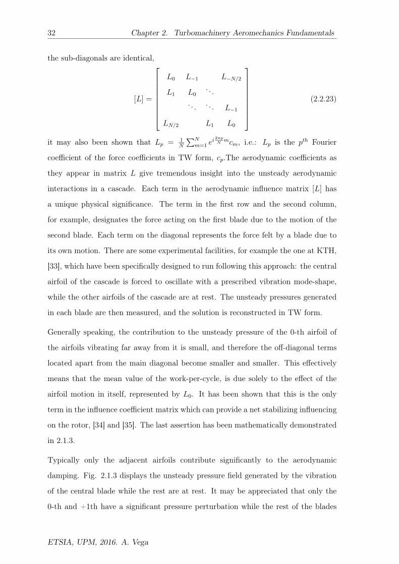
32 Chapter 2. Turbomachinery Aeromechanics Fundamentals
the sub-diagonals are identical,
[L] =
L0 L−1 L−N/2
L1 L0. . .
. . . . . . L−1
LN/2 L1 L0
(2.2.23)
it may also been shown that Lp = 1N
∑Nm=1 e
i 2πpNmcm, i.e.: Lp is the pth Fourier
coefficient of the force coefficients in TW form, cp.The aerodynamic coefficients as
they appear in matrix L give tremendous insight into the unsteady aerodynamic
interactions in a cascade. Each term in the aerodynamic influence matrix [L] has
a unique physical significance. The term in the first row and the second column,
for example, designates the force acting on the first blade due to the motion of the
second blade. Each term on the diagonal represents the force felt by a blade due to
its own motion. There are some experimental facilities, for example the one at KTH,
[33], which have been specifically designed to run following this approach: the central
airfoil of the cascade is forced to oscillate with a prescribed vibration mode-shape,
while the other airfoils of the cascade are at rest. The unsteady pressures generated
in each blade are then measured, and the solution is reconstructed in TW form.
Generally speaking, the contribution to the unsteady pressure of the 0-th airfoil of
the airfoils vibrating far away from it is small, and therefore the off-diagonal terms
located apart from the main diagonal become smaller and smaller. This effectively
means that the mean value of the work-per-cycle, is due solely to the effect of the
airfoil motion in itself, represented by L0. It has been shown that this is the only
term in the influence coefficient matrix which can provide a net stabilizing influencing
on the rotor, [34] and [35]. The last assertion has been mathematically demonstrated
in 2.1.3.
Typically only the adjacent airfoils contribute significantly to the aerodynamic
damping. Fig. 2.1.3 displays the unsteady pressure field generated by the vibration
of the central blade while the rest are at rest. It may be appreciated that only the
0-th and +1th have a significant pressure perturbation while the rest of the blades
ETSIA, UPM, 2016. A. Vega

2.3. Aerodynamic Damping Computational Methods 33
remain unperturbed. From a mathematical point of view this means that L0 6= 0 and
L1 6= 0 while the rest of the terms of matrix L are negligible in first approximation.
2.3 Aerodynamic Damping Computational Methods
2.3.1 Coupled methods
Fully coupled methods try to mimic as close as possible the physics of the fluid-
structure problem making use of the less possible number of approximations. Ideally
fully coupled methods should simultaneously march in time the RANS equations
for the fluid and the elasticity equations for the structure, exchanging the solvers
the aerodynamic forces (static pressure and viscous stresses) and the structure
displacements at the interface. RANS equations had to be solved in moving grids,
which are continuously recomputed every time step to accommodate the structure
displacements. [36, 37, 38, 39, 40, 41]
Fully coupled methods are computationally intensive for the simulation of time
periodic or quasi-periodic turbomachinery problems, not only because of the system
of equations has to be marched in time for many (at least ten) fundamental periods
to reach a periodic solution, but because the whole wheel has to be included in the
simulation, both in the fluid and the structure. As a consequence, even today, the
resulting problem is hardly manageable in a design environment. Typically turbine or
compressor rotors are made up of about 100 airfoils, if every passage were discretised
with a one million node grid, which is usually considered as a marginal resolution for
a purely aerodynamic simulation, the mesh of the whole annulus would have about
100 million points and should be marched in time for 10-100 fundamental periods.
Several methods exist to reduce the computational time of fully coupled methods
with a negligible impact on the solution accuracy.
1. Use of a subset of nominal modes. In this approach, the structural
natural frequencies, ωr, and mode-shapes, φr(x), of the structure are computed
ETSIA, UPM, 2016. A. Vega
34 Chapter 2. Turbomachinery Aeromechanics Fundamentals
taking into account the cyclic symmetry of the problem in a a pre-processing
step and stored. The structure is discretised in a single sector and the mode-
shapes and natural frequencies computed imposing cyclic symmetry boundary
conditions, which are the counter part of the phase-lagged boundary conditions
in unsteady aerodynamic simulations. The displacements of the whole structure
are expanded in the basis of the structural modes, and the time evolution of
the modal deflections, ηr, is computed as
mrd2ηrdt2
+ ω2rηr =
ˆΣ
φr(x).f(x) dσ (2.3.1)
where the right hand side represents the modal force, which is obtained,
projecting the aerodynamics forces on the airfoil surface, f = −(−p ¯I + ¯τv).n,
onto the mode-shapes, which are usually normalised to deliver a modal mass,
mr = 1. The structural mode-shapes are interpolated from the FE mesh onto
the aerodynamic mesh, since both grids are unlikely to be coincident. The
cost of evaluating the time response of the structure becomes negligible, since
only a few modes of the order of hundreds at most, need to be marched in
time. Mode-shapes are usually expressed in travelling-wave form [38] although
for simplified problems sometimes the individual blade formulation is preferred
[41]. Initial boundary conditions are selected in such a way that all the modes
of the structure are perturbed.
Damping is obtained tracking in time the modal amplitudes and computing the
logarithmic decrement, δ = ln(xn+1/xn), where xnand xn+1 are two consecutive
maxima in the amplitude of the modal deflection (see Fig. 2.3.1). It can be
shown that in the free vibration of a linear second order system:
mx+ cx+ kx = 0 (2.3.2)
the logarithmic decrement is
δ =2πξ√1− ξ2
(2.3.3)
where ξ = c/2πmω0, is the so-called critical damping ratio, and ω0 =√k/m,
is the purely structural natural angular frequency. Engineering systems are
ETSIA, UPM, 2016. A. Vega

2.3. Aerodynamic Damping Computational Methods 35
Normalised Time
0 2 4 6 8 10
Am
plit
ud
e
-1
-0.8
-0.6
-0.4
-0.2
0
0.2
0.4
0.6
0.8
1
Figure 2.3.1: Logarithmic decrement as a function of the normalised time
frequently lightly damped and ξ 1. Within this approximation δ ' 2πξ. The
non-dimensional eigenvalues of the system are:
ω =ω
ω0′= iξ ±
√1− ξ2 (2.3.4)
and therefore δ is a good approximation to the imaginary part of the eigenvalue,
that is, the non-dimensional damping.
2. Pre-Computed Aerodynamics. A second approach to reduce the cost of
the fully coupled methods is to pre-compute the aerodynamics. The standard
hypothesis is that the solution of the problem is harmonic, compute the
aerodynamics in travelling-wave form and translated or not into influence
coefficient form. The hypothesis that the flow is linear and that the unsteady
perturbations are proportional to the vibration amplitude is usually used.
Eventually the correction of the aerodynamic with the oscillating frequency
could be included but this approach is not usually followed. The resulting
problem can be cast in the form of an eigenvalue problem to determine the
stability [17] of the aeroelastic problem, or as an initial value problem which is
marched in time to find the final non-linear saturated solution [41].
ETSIA, UPM, 2016. A. Vega
36 Chapter 2. Turbomachinery Aeromechanics Fundamentals
2.3.2 Uncoupled methods
When the mass ratio of the system is high (µ 1), the aeroelastic modes and natural
frequencies of the bladed-disc are very similar to that of the in-vacuum structure.
The free response of the system consists in a slowly-varying envelope of the airfoil
amplitudes or of the bladed-disc modal coordinates. Under these conditions the most
efficient procedure is to prescribe the harmonic motion and frequency of the mode.
In this case, the computation of the aerodynamic damping reduces to the solution
of a purely unsteady aerodynamic problem where the displacements on the surface
of all the airfoils are given. This approach is simple and can be computationally
very efficient if used in combination with frequency domain solvers, either linear or
non-linear [42, 43, 44].
In this approach, airfoils are forced to oscillate at a specified mode, with constant
amplitude, frequency and IBPA [45]. Since the motion is given, the stability of the
system is quantified by the work performed within one cycle by the fluid in the
structure. With the standard criterion of signs, if the work is positive, it means that
the aerodynamic contribution stabilizes the motion, whereas if the work is negative,
the system is unstable and in a free vibration case the oscillation would be amplified.
The work exerted by the unsteady flow-field onto the blades is calculated as the result
of the application of the unsteady aerodynamic pressure onto the blade displacements.
2.3.2.1 Discussion
It is interesting to use the analytical solution of free-vibration of the 2nd order system
represented by Eq. 2.3.2. The energy dissipated per cycle by the viscous damping can
be computed by evaluating the difference of the total energy (kinetic and potential)
of the system between two consecutive peaks of the response, xn and xn+1, (see Fig.
2.3.1), i.e.: Wcycle = En −En+1, where En = 12x2n + 1
2x2n. The non-dimensional Wcycle
is:
Wcycle =Wcycle
mω20x
2n
=1
2
(1− e−
4πξ√1−ξ2
)(2.3.5)
ETSIA, UPM, 2016. A. Vega

2.3. Aerodynamic Damping Computational Methods 37
where obviously, since the problem is linear there is not a characteristic vibration
amplitude. The non-dimensional Wcycle is directly related with the logarithmic
decrement as Wcycle = 12
(1− e−δ
). If we further assume that ξ 1, then
Wcycle ' 2πξ .
If we assume, like in the uncoupled approach, that the motion of the system is
harmonic, with the angular frequency of the purely structural problem, ω0, theWcycle
of the viscous damping would be computed as:
Wcycle =1
mω20x
20
ˆ T=2π/ω0
0
cx2dt = 2πξ (2.3.6)
where the motion is given by x = x0 sinω0t, and obviously the rest of the forces have
a null contribution to the Wcycle, since they are conservative.
This effectively means that, if the aerodynamics is linear, as the viscous damping is,
the difference in computing the Wcycle, using a fully coupled method (Eq. 2.3.5) and
an uncoupled approach (Eq. 2.3.6) is an error of second order in ξ, if ξ 1,
W uncoupledcycle = W coupled
cycle + 0(ξ2) (2.3.7)
The coupled method is able to account for the small shift in frequency due to the
aerodynamics; the actual non-dimensional vibration frequency of the 2nd order system
is ω =√
1− ξ2, which is the origin of the difference. Summarising, if ξ 1 (or µ1),
the use of an uncoupled approach is well justified. The comparison between coupled
and uncoupled approaches is sometimes misleading, since it is mixed up with the
fluid model. Fully coupled methods are usually used in conjunction with the URANS
equations , whereas uncoupled methods are based on the use of linearised frequency
domain solvers. The linearity or not of the unsteady aerodynamics with respect the
vibration amplitude is a conceptually different issue from the coupling method, and
it will be discussed later on, but it practice has been difficult to separate in the
past. A proper comparison would require the use of uncoupled non-linear methods,
either in the time-domain, or in the frequency domain, with the recent development
of non-linear harmonic balance methods.
Apart from flutter stability, coupled methods are well suited to the study of limit-
ETSIA, UPM, 2016. A. Vega

38 Chapter 2. Turbomachinery Aeromechanics Fundamentals
cycle oscillations, where the vibration amplitude is saturated by nonlinearities, either
in the fluid, as it is the case sometimes if shock-waves are present, like in choke flutter,
or in the structure, where dry friction can play an important role. Time dependent
fully coupled methods are also attractive to deal with separated flows, and in general
aerodynamically driven instabilities, such as rotating stall and buffeting. In all these
cases the assumption that all the blades vibrate with constant amplitude and IBPA
does not usually hold, and the vibration frequency is not known a priori either.
Up to now only systems with a single active mode has been considered. Uncoupled
methods work in a mode-by-mode basis and therefore there are not suitable to account
for mode interaction. Mode interaction can occur both, in the linear (like in flutter
of vane packets [17]), and non-linear (friction saturation [41] ) regimes, but it any
case the modes need to be close enough in terms of frequency to interact among
them. This type of analysis requires the use of fully coupled methods, even if the
aerodynamics is linear.
ETSIA, UPM, 2016. A. Vega

Chapter 3
Fundamentals of Unsteady
Aerodynamics
It is during our darkest moments
that we must focus to see the light
Aristotle Onassis
Contents
3.1 Context . . . . . . . . . . . . . . . . . . . . . . . . . . . . . 40
3.2 Planar Waves in the Euler Equations . . . . . . . . . . . 42
3.3 Unsteady Pressure Generation: The Role of Vorticity . 50
3.4 Unsteady Pressure Generation: The Role of Apparent
Mass . . . . . . . . . . . . . . . . . . . . . . . . . . . . . . . 53
3.5 Unsteady Aerodynamics of Oscillating Flat Plate Cas-
cades . . . . . . . . . . . . . . . . . . . . . . . . . . . . . . 57
3.6 Laminar Boundary with an Oscillating Free Stream . . 59
3.7 Basic Non-dimensional Analysis of Unsteady Aerody-
namics . . . . . . . . . . . . . . . . . . . . . . . . . . . . . . 61
39
40 Chapter 3. Fundamentals of Unsteady Aerodynamics
3.1 Context
Unsteady aerodynamics associated to oscillating airfoils is complex, and little can be
said with a large degree of generality. Computational methods based on the solution
of the linearized Navier-Stokes equations are widely used in the gas turbine industry,
and even fully non-linear unsteady methods are used for some specific problems. The
accuracy of computational methods is acceptable for most of the cases, especially
within the industry, where codes have been tuned for specific flows, however the
physical understanding of these flows is reduced.
Unsteady pressure distributions have little to do with steady pressure fields and the
variability is even larger. To begin with the base mean flow, it has a strong influence
on the perturbations. Steady aerodynamics of low-pressure turbines, which is a high
subsonic Mach number flow subject to a large turning, is completely different of
compressor aerodynamics that may even change dramatically from operating point
to operating point. Compressor flows have low turning but may include shock waves
at different positions.
When talking about unsteady fields, new parameters such as the reduced frequency,
the phasing between the vibration of neighbouring airfoils or the vibration mode-
shapes themselves appear, making the variability of the problem very large.
As a consequence of the complexity of the unsteady aerodynamic associated to
vibrating airfoils, and despite the advances in computational fluid dynamics (CFD)
and experimental methods, that have enabled flutter and forced response studies, an
analytical approach for understanding the basic mechanisms, and for prediction and
design is still forthcoming.
Most of the theoretical work in unsteady aerodynamics was performed during the
1920s and 1930s. One of the most important and significant of them, which is owned
by Theodorsen, [6], will be briefly reviewed in this thesis, and the main conclusions
applicable to vibrating airfoils will be highlighted with the final aim of showing
the state-of-the-art of the knowledge about the unsteady aerodynamic behaviour
of oscillating airfoils.
ETSIA, UPM, 2016. A. Vega

3.1. Context 41
The work of Wagner, [46], was the starting point of Theodorsen and some other
studies focused on understanding the unsteady flow field originated by an oscillating
airfoil. The main finding of Wagner was that the oscillatory motion generates a vortex
wake, which in turn affects the entire nature of the forces experienced by the airfoil.
Theodorsen’s [6] theory, is based on potential flow and the Kutta condition. He
developed a solution for the unsteady loads (lift and moment) on a flat plate
undergoing harmonic oscillations in both, torsion and translation, and he applied
the results to an analysis of the wing-flutter problem. Garrick, [47], extended
Theodorsen’s theory and calculated the drag/propulsion forces.
In the turbomachinery field, the unsteady phenomena are very complex and they
are a major concern in current designs [48], [49], [50], [51]. Some examples of
important unsteady phenomena are: the effects of aerodynamically induced and self-
excited blade vibrations on aeroelastic response and stability, the effects of blade row
interactions and turbulence on efficiency and noise generation, the effects of inlet flow
non-uniformities on compressor and engine aerodynamic stability, and the nature and
flow structure of general post-stall engine transients.
Several studies were carried out in the past with the aim of understanding
the unsteady flow phenomena and the development of theoretical procedures for
predicting such phenomena [20], [52], [51], [53]. The theory derived in the present
thesis follows an approach that combines the approaches of other authors, such as
[6, 7, 42], since it is a linear theory, for airfoils oscillating at small amplitudes in
high-subsonic flow, and the conclusions are derived from an asymptotic analysis of
the linearised equations. The difference now is that the theory presented includes
real airfoil profiles and viscosity effects, and that the practical conclusions extracted
here apply to a wider range of operating flow conditions (even transonic conditions,
with the presence of shock waves), and is valid for any vibration mode-shape.
ETSIA, UPM, 2016. A. Vega
42 Chapter 3. Fundamentals of Unsteady Aerodynamics
3.2 Planar Waves in the Euler Equations
The understanding of the unsteady compressible flow about an oscillating airfoil is
a daunting task. The objective of this section is to briefly remind key elements of
the one- and quasi-one-dimesional theory of compressible flows, which constitute the
building blocks of the understanding of more complex flows. Special attention is paid
to the realistic case in which the unsteady flow perturbations are small with respect
the base flow.
3.2.1 One-dimensional Flow
Let us consider an inviscid flow in a constant area duct, without heat addition,
subject to planar, or one-dimensional perturbations, at the inlet or the outlet. The
one-dimensional governing equations can be expressed as:
∂ρ
∂t+ u
∂p
∂x+ ρ
∂u
∂x= 0
ρ∂u
∂t+ ρu
∂u
∂x+
∂p
∂x= 0
∂s
∂t+ u
∂s
∂x= 0
(3.2.1)
which constitute, respectively, the mass, momentum and entropy equations. In order
to close the problem an expression for the entropy as a function of the state variables
is need, s = s(p, ρ). For a perfect ideal gas s = cv ln(p/ργ). The entropy equation
can then be written as:(∂p
∂t− a2∂ρ
∂t
)+ u
(∂p
∂x− a2 ∂ρ
∂x
)= 0 (3.2.2)
where a =√γp/ρ is the speed of sound. This system of equations can be written as:
∂V
∂t+ A(V)
∂V
∂x= 0 (3.2.3)
where VT = ρ, u, p. The problem can be diagonalized to obtain the characteristic
form of the equations. The entropy equation was already in diagonal form since
entropy is convected with fluid velocity and remains unchanged (Eq. 3.2.2) whereas
ETSIA, UPM, 2016. A. Vega

3.2. Planar Waves in the Euler Equations 43
the mass and momentum equations are recombined to yield:(∂p
∂t± ρ a∂u
∂t
)+ (u± a)
(∂p
∂x± ρ a∂u
∂x
)= 0, (3.2.4)
which represents the upstream and downstream propagation of acoustic waves, in the
case of a subsonic flow. The eigenvalues of the problem are: λ1,2 = u± a and λ3 = u.
Equations 3.2.2 and 3.2.4 can be linearised about a mean uniform flow. If we assume
that the flow can be decomposed as:
u = u0 + u′; ρ = ρ0 + ρ′; p = p0 + p′ (3.2.5)
where u0, ρ0, u0 are constants, and the perturbations are small, i.e.: p′ po, ρ′
ρ0, and u′ u0. The systems of equations 3.2.3 in diagonal form becomes:
∂C
∂t+ Λ0
∂C
∂x= 0 (3.2.6)
where
Λ0 =
u0 + a0 0 0
0 u0 − a0 0
0 0 u0
and C =
p′ + ρ0a0u
′
p′ − ρ0a0u′
p′ − a20ρ′
(3.2.7)
which represents a system of three independent linear waves propagating the
characteristic variables at three different speeds, u0 ± a0 and u0. Acoustic
perturbations propagate upstream and downstream (ifM0 < 1) with velocities u0±a0,
conserving p′±ρ0 a0 u′, while entropy is convected downstream with velocity u0. Note
that if the entropy is constant upstream, as it is the case of a 2D airfoil oscillating
in an inviscid flow, then s = s0 ∀t, and will not be possible to see entropy waves
propagating through the fluid.
3.2.2 Vorticity Equation
A complete vision of the unsteady aerodynamics basics is not possible without
resorting to the concept of vorticity, ~ω = ∇×v. Although vorticity is a two- or
three-dimensional concept, it is included here because of its relevance. The vorticity
ETSIA, UPM, 2016. A. Vega

44 Chapter 3. Fundamentals of Unsteady Aerodynamics
equation is obtained taking the curl of the momentum equation:
ρD(~ω/ρ)
Dt= ~ω.∇v −∇
(1
ρ
)×∇p+∇×
(1
ρ
)∇.τ ′ +∇× f
m
(3.2.8)
The second term of the right hand side (r.h.s.) is zero if p = p(ρ), being the case of
homeotropic flows (s = s0) a particular case. The third term of the r.h.s. is zero if
the flow is inviscid, since in this case the viscous stresses, τ ′, are null. The fourth
term of r.h.s. is zero if the body forces derive of a potential, U , i.e.: fm = −∇U.
Even in the case of the flow about a two-dimensional section corresponding to a rotor
blade rotating with constant angular velocity, ~Ω, this term vanishes since centrifugal
forces are conservative and the Coriolis forces are perpendicular to the section and do
not contribute to the non-null component of the vorticity, ωz. Therefore, Eq. 3.2.8
for and inviscid homeotropic flow reduces to:
ρD(~ω/ρ)
Dt= ~ω.∇v (3.2.9)
Moreover if the flow is two-dimensional, ~ω.∇v=0, and then the vorticity equation
dictates the convection of ωz/ρ. If we assume that the perturbations are small,
ωz = ωz0 + ω′z, and that the base flow is uniform and irrotational, ωz0 = 0, the
linearised vorticity equation becomes:
Dω′zDt
= 0 (3.2.10)
which estates that the vorticity perturbations are convected downstream in an inviscid
tow-dimensional flow. It is important to notice that this is true even if the Mach
number of the base flow is of order unity, M0 ∼ 0(1).
3.2.3 Quasi One-Dimensional Flow
All the key concepts outlined up to know are of great help to understand the
aerodynamics of oscillating airfoils, but they are still far away from a representative
model, even for conceptual studies. In this sub-section we address the problem of the
compressible isentropic unsteady flow moving through a slowly varying, both in time
and space, duct (see Fig. 3.2.1). The low reduced frequency limit, and the effect of
ETSIA, UPM, 2016. A. Vega

3.2. Planar Waves in the Euler Equations 45
Figure 3.2.1: Sketch of a slowly varying duct
the varying area, A(x, t), will be discussed.
If it is assumed the case in which the characteristic length in the axial direction of
the nozzle, lx ∼ L, is much larger than the corresponding in the orthogonal direction,
ly ∼ o(A1/2), then the axial velocity, u, is much larger than the transversal velocity,
v, v u, and then the motion is quasi one-dimensional. It can be shown that the
governing equations of the problem are slight variant of that of the one-dimensional
problem . The mass conservation in this case is:
∂(ρA)
∂t+∂(ρ uA)
∂x= 0 (3.2.11)
The momentum and entropy equations remain the same within this approximation.
The new system of equations can be linearized about a mean flow decomposing the
flow as:
u = u0 + u′; ρ = ρ0 + ρ′; p = p0 + p′ (3.2.12)
where u0(x), ρ0(x), u0(x) represent the mean flow and in general depend of the
position, but we will assume that are constant. The basic hypothesis is that the area
variations are small, ∆Ax/A0 1. The linearised mass and momentum equations
using the hypothesis of isentropy (p− p0 = (ρ− ρ0)a20) become:
∂p′
∂t+ ρ0 a
20
[At + u0 Ax +
∂u′
∂x
]+ u0
∂p′
∂x= 0 (3.2.13)
∂u′
∂t+ u0
∂u′
∂x= − 1
ρ0
∂p′
∂x(3.2.14)
where At = 1A0
∂A∂t
and Ax = 1A0
∂A∂x. The previous system of equations can be
ETSIA, UPM, 2016. A. Vega
46 Chapter 3. Fundamentals of Unsteady Aerodynamics
diagonalised, yielding:
∂
∂t(p′ ± ρ0 a0 u) + (u0 ± a0)
∂
∂x(p′ ± ρ0 a0 u) = −ρ0 a
20
(u0 Ax + At
)(3.2.15)
Previous equation is identical to that obtain for one-dimensional flow (Eq. 3.2.4),
with the exception of the r.h.s. forcing term. This means that area variations,
eventually vibrations, give rise to acoustic perturbations, propagating upstream and
downstream, in the case of a subsonic flow, but not to entropy perturbations.
3.2.4 Order of Magnitude Estimates
The objective of this section is to use the simple model for the motion of a
compressible isentropic flow in a duct of area A, that changes as: A(x, t) =
A0 +A′(x) sinωt, to estimate which is the order of magnitude of the different terms of
the governing equations, to help to understand later on the mechanisms involved in
the pressure generation of an oscillating airfoil, and its magnitude. The momentum
equation and the estimate of the order of magnitude of its different terms can be
written as:∂u
∂t︸︷︷︸ + u∂u
∂x︸︷︷︸ +1
ρ
∂p
∂x︸︷︷︸ = 0
Uctc
U2c
L
∆pcρcL
(1) ↓ (2) ↓ (3) ↓trtc
O(1)∆pcρcU2
c
(3.2.16)
where Uc,tc, L, ∆pc and ρc are respectively the characteristics velocity, time, length,
pressure variation and density of the problem. In our problem, for instance if we
assume that the duct area changes with angular velocity, ω, then tc ∼ ω−1. The
residence, or through-flow time, tr, is defined as tr = L/Uc. The first row under the
momentum equation contains the estimate of the order of magnitude, the second row
is a label to shorten the reference to that term, whereas the last row contains the
relative order of magnitude with respect the term (2), that now is of order unity.
ETSIA, UPM, 2016. A. Vega

3.2. Planar Waves in the Euler Equations 47
Analogously the continuity equation reads:
∂p
∂t︸︷︷︸ + u∂p
∂x︸︷︷︸ + ρ a2∂u
∂x︸ ︷︷ ︸ = − ρ a2AtA0︸ ︷︷ ︸ − ρ a2u
AxA0︸ ︷︷ ︸
∆pctc
Uc∆pcL
ρca2cUcL
ρca2cδA
tc
ρca2cUcA
tc
(4) ↓ (5) ↓ (6) ↓ (7) ↓ (8) ↓
∆pcρca2
c
trtc
∆pcρca2
c
O(1) δAtrtc
δA
(3.2.17)
We will be discussing now the relative importance of the different terms as a function
of the characteristic time, or in other words the oscillation frequency, ω. A full
discussion of the problem is very involved, we will focus here in the low reduced
frequency limit, k = tr/tc = ωL/Uc 1.
Low reduced frequency limit (tr tc)
If the residence time is much smaller than the characteristic time, i.e.: tr tc ⇒
k 1, then:
• In the momentum equation, inertia terms, (1), are much smaller than the
convective terms , (1) (2), and therefore pressure and convective terms are
of the same order, (2) ∼ (3). We can then estimate the order of magnitude of
the pressure variations since, (2) ∼ (3) ⇒ ∆pcρcU2
c∼ O(1), or in other words, the
pressure variations are of the order of the dynamic head.
• In the continuity equation, inertia terms, (4), are also much smaller than the
convective terms (5) and (6). The order of magnitude of (5) with respect (6) is
M2c . If M2
c 1, then (5) (6) and we recover the incompressible limit.
• The unsteady forcing term, (7), is also much smaller than the steady one, (8),
and can be neglected in first approximation.
ETSIA, UPM, 2016. A. Vega

48 Chapter 3. Fundamentals of Unsteady Aerodynamics
The governing equations reduce in first approximation to that of the steady flow, the
time plays the role of a parameter, and the problem is said to be quasi-stationary:
u∂p
∂x+ ρ a2∂u
∂x= −ρ a2u
AxA0
u∂u
∂x+
1
ρ
∂p
∂x= 0
(3.2.18)
In the current analysis, we consider the case in which the area variations are small
with respect the characteristic area, δA/A0 1. The forcing term in the r.h.s. of
the continuity equation is small, and causes a small perturbation in the pressure,
p′0, and velocity, u′0, fields. To estimate the order of magnitude of the perturbations
associated to the area variation, we assume, to ease the presentation but without any
loss of generality, that the spatial variations of pressure and velocity of the base flow
are null, technically speaking that ∆px0 p′0 and ∆ux0 u′0. In this case the mass
and momentum equations for the perturbations with respect the base flow, and the
order of magnitude of the different terms are:
u0∂p′0∂x︸ ︷︷ ︸ + ρ0 a
20
∂u′0∂x︸ ︷︷ ︸ = − ρ0 a
20u0
AxA0︸ ︷︷ ︸
↓ ↓ ↓
u0p′0L
ρ0a20
u′0L
ρ0 a20u0
δAxL
(3.2.19)
u0∂u′0∂x︸ ︷︷ ︸ +
1
ρ0
∂p′0∂x︸ ︷︷ ︸ = 0
↓ ↓
u0u′0L
1
ρ0
p′0L
(3.2.20)
The conclusion is that, in low reduced frequency limit, the order of magnitude of the
quasi-steady perturbations are: u′0/u0 ∼ δAx and p′0/ρ0 a20 ∼ δAx, where the non-
dimensional spatial variation of the area, δAx(t), is a function of time. The result is
Mach number independent, provided that M0 ∼ 0(1), and the perturbations are in
phase with the displacements.
ETSIA, UPM, 2016. A. Vega
3.2. Planar Waves in the Euler Equations 49
The second order correction to the perturbations, p′1 and u′1, are obtained retaining
the previously neglected unsteady terms:
∂p′0∂t︸︷︷︸ + u0
∂p′1∂x︸ ︷︷ ︸ + ρ0 a
20
∂u′1∂x︸ ︷︷ ︸ = −ρ0 a
20
AtA0︸ ︷︷ ︸
ρcu20
δA
tcu0
∆p′1cL
ρa20
∆u′1cL
ρ0 a20
δA
tc
(1) ↓ (2) ↓ (3) ↓ (4) ↓
δAu2
0
a20
trtc
∆p′1cρc a2
0
∆u′1cu0
δAtrtc
(3.2.21)
∂u′0∂t︸︷︷︸ + u0
∂u′
∂x︸ ︷︷ ︸ +1
ρ0
∂p′
∂x︸ ︷︷ ︸ = 0
u0δA
tc
u0∆u′1cL
1
ρ0
∆p′1cL
(5) ↓ (6) ↓ (7) ↓
δAtrtc
∆u′1cu0
∆p′1cρ0u2
0
(3.2.22)
On the view of the two previous equations two particular cases could be distinguished:
1. M0 ∼ O(1). In this case u0 ∼ a0, and if (2) ∼ (3) (or (6) ∼ (7)), the order
of magnitude of the correction to the pressure perturbation is ∆p′1c ∼ ρ0 u0 u′1c,
then if make (2) ∼ (4), we can conclude that: ∆p′1c∆p′0c∼ u′1c
u′0c∼ tr
tc∼ k. Moreover, it
can be seen that this correction is out of phase with respect the displacement,
since it is generated by the At term, and then the phase of the solution, φ,
scales as tanφ ∼ k.
2. M0 O(1). In this case u0 a0: for this case, based on the idea that (5) ∼ (7)
, it is obtained that ∆p′1c ∼ ρ0 u20 δA
trtc, and since (3) ∼ (4) it is obtained
u′1cu0∼ δA tr
tc. The conclusions are the same than for the M0 ∼ O(1). The only
difference being that (1) ∼ (2) (3) and the flow is nearly incompressible.
ETSIA, UPM, 2016. A. Vega

50 Chapter 3. Fundamentals of Unsteady Aerodynamics
3.3 Unsteady Pressure Generation: The Role of
Vorticity
3.3.1 Kelvin’s circulation theorem
The kelvin’s circulation theorem states that, for an inviscid and incompressible fluid
of constant density in motion in presence of conservative body forces f = −∇U per
unit mass, the circulation when considering a closed fluid circuit (the same fluid
particles as time proceeds) is:
Γ =
ˆC(t)
u dx (3.3.1)
and it is independent of time. It is important to note that:
• Incompressibility is not essential for the theorem to fulfill.
• The theorem does not require the fluid region to be simply connected, i.e., it
does not require the dyed circuit C to be spannable by a surface S lying wholly
in the fluid.
The generation of lift on an airfoil
The shedding of a starting vortex is essential to the generation of lift of an airfoil.
Kelvin’s theorem can be used to understand why this is so. Kelvin’s circulation
theorem states that the time rate of change of circulation around a closed curve
consisting of the same particles is zero.
Figure 3.3.1 helps to explain the lift generation mechanism on an oscillating airfoil.
At time t after the airfoil started moving, the viscous forces and vorticity will be
confined to: i) a thin boundary layer on the airfoil, ii) a thin wake and iii) the rolled-
up “core” of the starting vortex. If it is sketched in a line in space at time t such that
the curve aecda encloses the airfoil but not the wake or the starting vortex, then the
circulation around aecda must be equal and opposite to that round abcea, since at
the initial time instant, the total circulation in the circuit abcd is zero.
ETSIA, UPM, 2016. A. Vega

3.3. Unsteady Pressure Generation: The Role of Vorticity 51
a
e
c
db
1
2
Figure 3.3.1: Generation of circulation by means of vortex shedding
As the airfoil starts to move, positive vorticity is shed in the form of a starting vortex.
By Stokes theorem, ˆS
ω n dS =
ˆC
u dx (3.3.2)
where S represents the airfoil surface and C the closed circuit abcea, this vorticity
gives a positive circulation around abcea (see red arrow 1 in Fig. 3.3.1), which in turn,
by Kelvin’s circulation theorem, leads to a negative circulation around aecda (see red
arrow 2 in Fig. 3.3.1). The vortex shedding continues until the circulation around the
airfoil is sufficient to make the main, irrotational flow smooth at the trailing edge, at
which stage no further net vorticity is shed into the wake from the boundary layers
on the upper and lower surfaces of the airfoil. Thereafter, the airfoil retains its final
“Kutta-Joukowski” value of the circulation.
According with the Kutta Joukovski lift theorem, if it is considered a flow which
is uniform at infinity with speed U0 in the x-direction, if the circulation generated
around a body is Γ, then the force on the body will be F = (0,−ρU0Γ). The next
section explains from a mathematical point of view the role of vorticity in the lift
generation on an oscillating airfoil.
ETSIA, UPM, 2016. A. Vega

52 Chapter 3. Fundamentals of Unsteady Aerodynamics
3.3.2 General Formulation of Acoustic Perturbations
Howe’s [54] showed that combining the continuity and momentum equations, and if
dissipation is neglected and the flow is homeotropic (s = s0), the following equation
for the pressure can be obtained:(D
Dt
(1
a2
D
Dt
)− 1
ρ∇ (ρ∇)
)H =
1
ρ∇. (ρω ∧ v) (3.3.3)
where H = CpT + 12v2 is the total enthalpy and ω represents the shed vorticity. For
an uniform base flow, ρ = ρ0, a = a0, v = v0, the pressure equation can be linearised
about the mean flow to yield:(1
a20
D2
Dt2−∇2
)(p′
ρ0
+ v0 u′)
= ∇. (ω′ ∧ v0) (3.3.4)
which is the equivalent to the classical 2nd order wave equation with a source term.
In this context, the sub-index “0” represent the mean flow and the super-index “ ′”
the perturbed variables. The previous expressions clearly shows that when there is a
vorticity in the flow (for example, due to the change in the apparent angle of attack
for an oscillating airfoil), which is convected downstream with the flow velocity, u, this
vorticity is the responsible of the generation of an additional pressure over the airfoil,
since it creates a perturbation p′
ρ0+ v0 u
′, which is governed by Eq. 3.3.4. This is the
ultimate reason for the propagation of pressure perturbations with the flow velocity,
as it will be shown later on. This equation can be used in combination with the
Stokes theorem to estimate the order of magnitude of the unsteady pressure created
by the shed vorticity. The contribution of the unsteady terms in Eq. 3.3.4 can be
assumed to be much smaller, or at most of the same order, than the convective terms
(i.e.: 1a20
D2
Dt2/ ∇2), if the reduced frequency based in the speed of sound ωc/a0 / 1.
In this case :
∇2
(p′
ρ0
)∼ ∆p′cρ0L2
c
, and ∇.(ω′ ∧ v0) ∼ ω′c UcLc
(3.3.5)
need to be of the same order. The Stokes theorem provides the order of magnitude
of the shed vorticity:
Γ =
˛u dx =
ˆ∑ ω dA (3.3.6)
ETSIA, UPM, 2016. A. Vega
3.4. Unsteady Pressure Generation: The Role of Apparent Mass 53
where it can be derived that Γ ∼ ω′c L2c . Since the force generated by the vorticity
onto the airfoils is F ′c ∼ ρUc Γ′ then, the order of magnitude for the unsteady pressure
is:
∆p′cρ0 Uc²
∼ ω′c UcUc∼ F ′cρ0 U2
c Lc∼ C ′L (3.3.7)
This effectively means that the non-dimensional unsteady pressure associated to the
vortex shedding, is proportional to the variation of the lift coefficient.
3.4 Unsteady Pressure Generation: The Role of
Apparent Mass
The objective of this section is to qualitatively describe the effect on the unsteady
aerodynamics of the so-called apparent or virtual mass. To better present this idea,
and to ease the formulation, the fluid is supposed to be inviscid and incompressible.
Although this is a strong idealization with respect a real case, yet several and useful
results can be obtained. The purpose of this sub-section is to discuss this effect in
the context of oscillating airfoils.
3.4.1 Incompressible flow equations
The governing equations of the motion for an inviscid and incompressible flow reduce
to:
∇ · u = 0
ρ∂u
∂t+ ρ (u · ∇)u +∇p = 0
(3.4.1)
Applying the curl operator to the momentum equation, and taking into account that:
(u · ∇)u =1
2∇u2 + u ∧ ω (3.4.2)
where ω = ∇ ∧ u is the vorticity, the following expression is obtained for the
momentum equation:
∂ω
∂t+∇∧ (ω ∧ u) = 0 (3.4.3)
ETSIA, UPM, 2016. A. Vega

54 Chapter 3. Fundamentals of Unsteady Aerodynamics
The previous equation can be written as:
∂ω
∂t+ (u · ∇)ω = (ω · ∇)u (3.4.4)
It can be extracted from the last expression that for an ideal, steady, two-dimensional
flow, it is (u · ∇)ω = 0, and consequently, the vorticity is constant along a streamline,
which in fact means that the vorticity propagates with the convection velocity u. It
is important to note that the vorticity does not exist for a one-dimensional problem,
since it is by definition a two-dimensional concept.
For an irrotational flow (ω = 0) in any connected region, the velocity potential, φ, is
defined as:
u = ∇φ (3.4.5)
The continuity and momentum equations can be written in terms of the potential
velocity as:
∇2φ = 0 (3.4.6)
ρ∂
∂t∇φ+
ρ
2∇ |u|2 = −∇p (3.4.7)
The momentum equation can be written as:
∇(∂φ
∂t+
1
2|u|2 +
p
ρ) = 0 (3.4.8)
which leads to the Bernoulli equation:
∂φ
∂t+
1
2|u|2 +
p
ρ= F (t) (3.4.9)
Equations 3.4.6 and 3.4.9, together with the appropriate boundary conditions, define
the unsteady motion of an incompressible irrotational flow.
3.4.2 Inviscid Moving Sphere
Let us consider a sphere moving with velocity U(t), and a control volume, Ω,
surrounding it (see Fig. 3.4.1), the total kinetic energy of the flow surrounding the
ETSIA, UPM, 2016. A. Vega
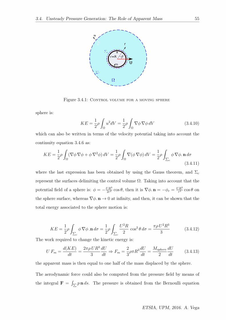
3.4. Unsteady Pressure Generation: The Role of Apparent Mass 55
Figure 3.4.1: Control volume for a moving sphere
sphere is:
KE =1
2ρ
ˆΩ
u2dV =1
2ρ
ˆΩ
∇φ∇φ dV (3.4.10)
which can also be written in terms of the velocity potential taking into account the
continuity equation 3.4.6 as:
KE =1
2ρ
ˆΩ
(∇φ∇φ+ φ∇2φ) dV =1
2ρ
ˆΩ
∇(φ∇φ) dV =1
2ρ
ˆ∑c
φ∇φ.n dσ
(3.4.11)
where the last expression has been obtained by using the Gauss theorem, and Σc
represent the surfaces delimiting the control volume Ω. Taking into account that the
potential field of a sphere is: φ = −UR3
2r2cos θ, then it is ∇φ.n = −φr = UR3
r3cos θ on
the sphere surface, whereas ∇φ.n→ 0 at infinity, and then, it can be shown that the
total energy associated to the sphere motion is:
KE =1
2ρ
ˆ∑c
φ∇φ .n dσ =1
2ρ
ˆ∑c
U2R
2cos2 θ dσ =
πρU2R3
3(3.4.12)
The work required to change the kinetic energy is:
U Fm =d(KE)
dt=
2πρUR3
3
dU
dt⇒ Fm =
2
3ρπR3dU
dt=Msphere
2
dU
dt(3.4.13)
the apparent mass is then equal to one half of the mass displaced by the sphere.
The aerodynamic force could also be computed from the pressure field by means of
the integral F =´∑ pn ds. The pressure is obtained from the Bernoulli equation
ETSIA, UPM, 2016. A. Vega
56 Chapter 3. Fundamentals of Unsteady Aerodynamics
3.4.9:
φt +1
2(∇φ)2 +
p
ρ=p∞ρ∞
(3.4.14)
where it has been introduced that when r →∞⇒ φt → 0 and ∇φ→ 0. Taking into
account that:
φt = − R3
2 r2
dU
dtcos θ and v2 = (∇φ)2 = φ2
r+
(φθr
)2
=
(U R3
r3
)2
cos2 θ+
(U R3
2r3
)2
sin2 θ
(3.4.15)
the aerodynamic force can be written as:
Fxρ
= −ˆ∑c,sphere
(φt +
1
2(∇φ)2
)cos θ dσ (3.4.16)
It can be shown that:ˆ∑c,sphere
φt cos θ dσ =πR3
3
dU
dt
ˆ π
0
d(cos3 θ) andˆ∑c,sphere
1
2(∇φ)2 cos θ dσ = 0
(3.4.17)
and then, the following expression for the aerodynamic force is obtained:
Fx =d
dt
ˆΩ
ρv dΩ = ρ
ˆ∑c
∂φ
∂tn dσ =
2
3ρπR3dU
dt. (3.4.18)
Saffman [55] express the aerodynamic force due to the flow about a moving body
without circulation (the virtual mass contribution) as F = ρ ddtIb, where Ib =
´Σφn dσ, which, as it can be readily seen, is nothing else that the contribution
of the inertia of the fluid.
These forces are always in-phase with the displacement, out-of-phase with the
velocity, and in the case of an harmonic motion, the net contribution to the work-
per-cycle of the inertia terms is zero. The order of magnitude of the inertia forces,
Fc, of the harmonic motion (δ = δmax sin(ωt)) of a body in an inviscid flow is
Fc ∼ ρR3δmaxω2, which in non-dimensional terms becomes:
FcρU2∞R
2∼ δnax
Rk2 (3.4.19)
where U∞ is the free-stream velocity and k = ωR/U∞ the reduced frequency. It can
be anticipated that inertia contribution to the unsteady pressure can be neglected if
k 1, and that, what is more, its contribution to the work-per-cycle is zero.
ETSIA, UPM, 2016. A. Vega

3.5. Unsteady Aerodynamics of Oscillating Flat Plate Cascades 57
3.5 Unsteady Aerodynamics of Oscillating Flat
Plate Cascades
Whitehead [56, 57] developed a method of calculation for linearised two-dimensional
subsonic unsteady flow through a cascade of flat plates operating at zero incidence.
The cascade, schematically represented in Fig. 3.5.1, is defined by a blade spacing,
s, a stagger angle θ , and an inlet Mach number, M . His method is suitable for
calculation of forced and self-excited vibration of the blades, and for the generation,
transmission, and reflection of acoustic waves by a cascade. The assumptions of his
analysis were:
• The flow is two-dimensional and isentropic. The bending modes of the blades
are represented by a translation motion, and the torsional modes by a rotation
about a known axis
• The blades are not stalled, so that the flow always follows the blade surface
• The blades are treated as flat plates and then, the effect of the camber an the
thickness are not taken into account.
• The blades operate at zero mean incidence.
• The amplitude of the perturbations is small, and then:
1. The wakes of the blades, which are vortex sheets whose strength varies
sinusoidally with distance from the trailing edge, can be assumed to be
straight
2. The governing equations are linear, and then any two solutions for the
perturbation can be superposed to obtain a third solution.
• All the blades oscillate with the same angular frequency, ω, and with a constant
phase change between each blade and its neighbour, σ.
ETSIA, UPM, 2016. A. Vega

58 Chapter 3. Fundamentals of Unsteady Aerodynamics
c
s
Figure 3.5.1: Sketch of the Whitehead’s cascade
• No viscosity effects are retained, and the Kutta-Joukowski condition at the
trailing edges of the blades is satisfied.
He found two kinds of acoustic resonances, one corresponding of an annular duct
without blades, and the other in the passages between the blades. He obtained
conditions for an acoustic wave to propagate, based on the angle between the wave-
fronts (lines of constant pressure) and the cascade direction:
sin ζ =Ω− 2πn
η s(3.5.1)
where Ω = σ − ωsa
1βM sin θ, β = 1√
1−M2 , a is the speed of sound, n is an integer,
and η = ωaβ
. Note that in Fig. 3.5.1 the propagation perturbations are represented
by pairs of arrows departing from both, the leading edge and the trailing edge of the
plate.
For a given cascade geometry, reduced frequency k = ωc/U , and Mach number, M ,
the range of σ within the perturbations do not decay and propagate at constant
ETSIA, UPM, 2016. A. Vega

3.6. Laminar Boundary with an Oscillating Free Stream 59
σ
Subresonant Subresonant
Superresonant
−180 −120 −60 0 60 120 1800
0.2
0.4
0.6
0.8
M
k=5
σ
Subresonant Subresonant
Superresonant
−120 −60 0 60 120 180−1800
2
4
6
8
10
k
M=0.5
Figure 3.5.2: Superresonant and subresonant regions as a function of theIBPA for constant reduced frequency and Mach number, left and rightrespectively.
amplitude is given by:
s
ck
M
1−M2
(M sin θ −
√1−M2 cos2 θ
)< σ <
s
ck
M
1−M2
(M sin θ +
√1−M2 cos2 θ
).
(3.5.2)
This region is called superresonant (see Fig. 3.5.2). Outside of this range of IBPAs
the perturbations decay and the solution is said to be subresonant. The region
of superresonant IBPA grows with the reduced frequency and the Mach number.
The separation between the propagating and non-propagating solutions are named
resonances. Solvers usually experience problem at these regions since high responses
at the inlet perturbations are observed. At the point of appearance of the acoustic
waves ζ = ±90ş, so that the direction of energy propagation is along the cascade.
This is a resonance condition, and also corresponds to the cut-off condition discussed
by Tyler and Soffrin [58].
3.6 Laminar Boundary with an Oscillating Free
Stream
The problem of understanding the unsteady behavior of a boundary layer subject
to fluctuations in the external flow is very important and has been the object of
ETSIA, UPM, 2016. A. Vega

60 Chapter 3. Fundamentals of Unsteady Aerodynamics
several studies [59, 60, 61, 62]. Here, the solution obtained by Lighthill [59] is briefly
reviewed. Lighthill obtained an analytical solution for the laminar boundary layer
in two-dimensional flow about a flat plate, when the velocity of the oncoming flow
relative to the body oscillates in magnitude but not in direction. He studied the
limiting cases of high and low oscillation frequencies, ω.
Lighthill obtained expressions for the reduced skin friction coefficient and the phase
angle between the external velocity and the wall shear for the cases in which
k = ωx/V∞ 1 and k 1, where x is the distance from the leading edge and
V∞ the free stream velocity. He obtained that there is a phase shift between the force
and the movement, due to the viscous terms. The main conclusions he obtained are
the following:
• The maximum skin friction at any point anticipate the maximum of the stream
velocity, because the pressure gradient needed to speed up the main stream
locally produces a given percentage increase in the slow flow near the wall
sooner than it can do so in the main stream itself.
• For each point on the body surface there is a critical reduced frequency, k0 = 0.6,
such that:
– If k > k0: the oscillations are to a close approximation ordinary “shear
waves” unaffected by the mean flow; the phase advance in the skin friction
is then 45ş
– If k < k0: the oscillations are closely approximated as the sum of
parts proportional to the instantaneous velocity and acceleration of the
oncoming stream; the phase advance, φ, in the skin friction is then
tanφ = k/k0.
Figure 3.6.1, extracted from [62], shows the computed phase angle (between the
wall shear stress and external velocity) variation with reduced frequency ωx/u0 for
a laminar flat-plate flow. It is concluded that for low reduced frequencies (k 1)
ETSIA, UPM, 2016. A. Vega
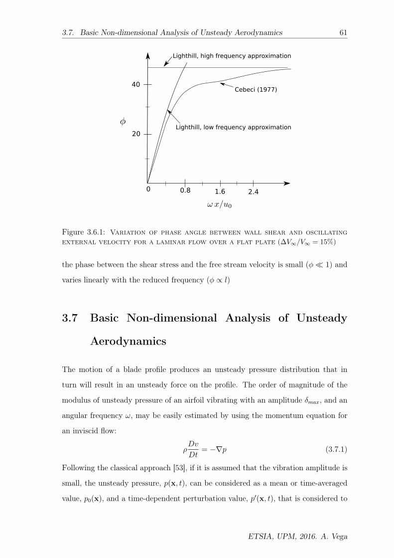
3.7. Basic Non-dimensional Analysis of Unsteady Aerodynamics 61
0 0.8 1.6 2.4
20
40
Lighthill, high frequency approximation
Lighthill, low frequency approximation
Cebeci (1977)
Figure 3.6.1: Variation of phase angle between wall shear and oscillatingexternal velocity for a laminar flow over a flat plate (∆V∞/V∞ = 15%)
the phase between the shear stress and the free stream velocity is small (φ 1) and
varies linearly with the reduced frequency (φ ∝ l)
3.7 Basic Non-dimensional Analysis of Unsteady
Aerodynamics
The motion of a blade profile produces an unsteady pressure distribution that in
turn will result in an unsteady force on the profile. The order of magnitude of the
modulus of unsteady pressure of an airfoil vibrating with an amplitude δmax, and an
angular frequency ω, may be easily estimated by using the momentum equation for
an inviscid flow:
ρDv
Dt= −∇p (3.7.1)
Following the classical approach [53], if it is assumed that the vibration amplitude is
small, the unsteady pressure, p(x, t), can be considered as a mean or time-averaged
value, p0(x), and a time-dependent perturbation value, p′(x, t), that is considered to
ETSIA, UPM, 2016. A. Vega
62 Chapter 3. Fundamentals of Unsteady Aerodynamics
be harmonic. According with this, the unsteady pressure can be expressed as:
p(x, t) = p0(x) + p′(x, t) (3.7.2)
The flow may be decomposed in a similar way as:
v(x, t) = v0(x) + v′(x, t) (3.7.3)
where the sub-index 0 denotes the mean flow, and the prime the unsteady perturbed
variables. Introducing the expressions 3.7.2 and 3.7.3 in Eq. 3.7.1, the order of
magnitude of the unsteady perturbation, ∆pc, may be estimated as:
∆pc ∼ ρcUcωδmaxmax(1, k) (3.7.4)
were ρ∞ and U∞ are the density and the velocity of the free stream, respectively.
Consequently, the order of magnitude of the unsteady force in the airfoil is then:
F a ∼ ρcUcωδmaxS = Fc (3.7.5)
where S is the airfoil surface. As it was shown by Crawley, [63], if it is considered a
cascade of vibrating airfoils, the unsteady forced in the ith-airfoil may be expressed
as:
F ai = FcF (k, σ, t) (3.7.6)
The most distinctive feature of the unsteady aerodynamics of vibrating airfoils in
turbomachinery is that the unsteady force in the ith airfoil depends on the motion of
all the airfoils, qj:
F ai = FcFj(k, q1, q2, ..., qj, ..., qN , t) (3.7.7)
In Chapter 1, it was explained that in the particular case that the airfoils motion is
harmonic in time, and that all the airfoils move with a common inter-blade phase
angle, σn = 2πnN
, the displacement of the airfoil ith is qi = qnej(iσn+ωt) , and then the
force in the ith airfoil may be expressed as a summation of the contribution of the
different temporal and spatial harmonics:
F ai = Re(Fc
∑ω
∑n
Fn,ω(q)ej(iσn+ωt)) (3.7.8)
ETSIA, UPM, 2016. A. Vega

3.7. Basic Non-dimensional Analysis of Unsteady Aerodynamics 63
nVw
Σ
Figure 3.7.1: Moving surface of an oscillating airfoil
As it has been previously mentioned, under the assumption that the unsteady
perturbations are much smaller than the mean flow, p′(x, t) p(x), the unsteady
aerodynamics is linear. According with this, a necessary condition is then that:
∆pcpc∼ ρ∞U∞ωδmax
pc∼M2k
δmaxc
(3.7.9)
where c is the blade chord. It can be easily seen that the condition for having linear
flow is the blade displacements to be small enough, δmax/c 1.
In the present case, it has been considered that the solution is harmonic in time,
i.e.: composed in first approximation of a single harmonic, corresponding with the
vibration frequency. The contribution of higher harmonics is negligible since they
are the results of non-linear interactions and then, the force in the airfoil i may be
expressed as:
F ai = Re(Fc
∑n
Fn(q)ej(iσn+ωt)) (3.7.10)
The unsteady pressure is also proportional to the vibration amplitude, and therefore
it is interesting to scale the blade force with δmax:
F ai = Re(Fc/δmax
∑n
fn(ω)qnej(iσn+ωt)) (3.7.11)
The unsteady force Fourier coefficients, fn , depend on the reduced frequency and
the inter-blade phase angle, fn(k, σ), and are complex numbers.
3.7.1 Aerodynamic work-per-Cycle
The work per oscillation cycle exerted by the fluid on the profile determines whether
the flow has a stabilizing or a destabilizing character; in case of the fluid putting work
ETSIA, UPM, 2016. A. Vega
64 Chapter 3. Fundamentals of Unsteady Aerodynamics
on the structure the situation is referred to as unstable, and the sign criteria used in
this thesis refers the work as positive in such cases. The work-per-cycle performed
by the aerodynamic forces can be calculated as:
Waero =
ˆT
(ˆ∑ p(x, t) ·Vω·n · dA
)dt (3.7.12)
where p represents the unsteady pressure, Vw the airfoil motion, and∑
the airfoil
surface (see Fig. 3.7.1). If it is assumed that there is no spatial dependency of the
pressure and airfoil motion, i.e.: p = p(t), and the same is true for the airfoil motion,
Vω(x, t) = Vω(t), then the previous formula is simplified and can be written as:
Waero =
ˆT
faero(t) ·Vω(t) dt (3.7.13)
If we assume now that the motion is harmonic in time, xw = xeiωt ⇒ Vw(x, t) =
iωxweiωt and f = feiωt, then the work per cycle becomes Wcycle = π(faero,I xR −
faero,RxI). If we set the time origin such as x = xR cosωt, then:
Wcycle = πfaero,I xR (3.7.14)
This means that the aerodynamic work per cycle is associated to the imaginary, or
out-of-phase, component of the forces. In the general case that the pressure and the
mode-shape are a function of the position, the same result may be obtained, if the
order of the spatial and temporal integral is exchanged.
If it is recovered the expression obtained in the Chapter 2 for the aerodynamic forces,
2.1.7, an expression for the Wcycle as a function of the influence coefficients can be
obtained. In general, the ICs are not symmetric, ∆l∗+ 6= 0 and ∆l∗− 6= 0, in which
case the expression of the aerodynamic forces is:
faero = l0 + ∆l+ cosσ −∆l−∗ sinσ + i(l∗0 + ∆l∗+ cosσ + ∆l− sinσ
)(3.7.15)
Then, the aerodynamic work per cycle can be written in terms of the influence
coefficients as:
Wcycle =Wcycle
12πρcv2
cδ2c
= π ·(l∗0 + ∆l∗+ cosσ + ∆l− sinσ
)xR (3.7.16)
where it can be clearly seen that the destabilizing effect comes form the neighouring
ETSIA, UPM, 2016. A. Vega

3.7. Basic Non-dimensional Analysis of Unsteady Aerodynamics 65
airfoils, while the contribution to the work per cycle of the airfoil itself is always
of stable nature. It can also be seen that the mean value of the work per cycle is
associated to the effect of the oscillating airfoil in itself. This expression has a deep
physical insight and will be exploited in the next chapters of the thesis.
3.7.1.1 Non dimensional aerodynamic work
The non-dimensionalization of the aerodynamic work per cycle is treated deeply in
this thesis, the basics and the classical approach are presented here just to provide
a complete vision of the unsteady aerodynamic problem. The aerodynamic work-
per-cycle, Waero , may be scaled from a purely aerodynamic point of view using the
unsteady pressure, estimated in Eq. 3.7.4, as:
Θ =Wcycle
2π · ρcUc · ω · δ2max ·max(1, k) · S
(3.7.17)
Then, according with the classical approach, the non-dimensional aerodynamic work,
Θ, depends on the following parameters:
Θ = Θ(k, Mode− shape, δ
c, M, Re, αin) (3.7.18)
where it can be seen that the non-dimensional aerodynamic work depends on the
vibration frequency, the mode-shape and the steady flow-field. The understanding of
the dependence of the non-dimensional aerodynamic work with these parameters will
be the focus of this thesis. A short overview of the common knowledge up to these
days is presented here:
• The reduced frequency, k, is usually used as a target design criterion to fix flutter
problems, both in the conceptual and in the detailed design phase. Natural
frequencies are raised either increasing the blade chord, the thickness, or both.
The most powerful mechanism of controlling the reduced frequency is the blade
aspect ratio.
• Aerodynamic work sensitivity with the mode-shape is much larger. The
aerodynamic work per cycle,Wcycle, changes strongly with the inter-blade phase
ETSIA, UPM, 2016. A. Vega

66 Chapter 3. Fundamentals of Unsteady Aerodynamics
angle, IBPA, but even when focusing in the most critical IBPA, which is the
minimum of theWcycle−IBPA curves and represents the least stable situation,
the position of the center of torsion of the airfoil may dramatically change the
aerodynamic work. The most clear example is the change in aerodynamic work
per cycle between flap and edge modes, as it can be seen in Fig. 3.7.2, which
represent the non-dimensional work per cycle curves as a function of the IBPA
for the flap and edge modes for an LPT for a reduced frequency of k = 0.1.
It can be seen that, for the same reduced frequency, the flap configuration is
much more unstable (about five times) than the edge configuration, and that
the sign of the IBPA at which occurs the minimum of the work per cycle is
the opposite. The location of the torsion center must be carefully controlled to
drive the designs in the right direction.
• Aerodynamic work is, in general, insensitive to the vibration amplitude except
in particular non-linear problems, such as shock flutter, where the aerodynamic
work may even change of sign with the vibration amplitude.
• Steady aerodynamic flow-field obviously change the aerodynamic work per
cycle:
– For a given application the variability of the Mach number is reduced, since
this is fixed by purely aerodynamic criteria, and it is not a free parameter.
– Sensitivity of the aerodynamic work to the Reynolds number is small, since
the unsteady pressures caused by the airfoil motion are mainly an inviscid
phenomenon. An exception is the case of compressor stall flutter, where
separation is controlled by viscous effects.
– Incidence change caused by shaft speed variation may heavily change
the flow-field and hence the aerodynamic work per cycle, especially in
compressors.
The aerodynamic work may also be scaled assuming that it will take part of the airfoil
motion equations, which for a single degree of freedom system take the following form:
ETSIA, UPM, 2016. A. Vega

3.7. Basic Non-dimensional Analysis of Unsteady Aerodynamics 67
−180 −135 −90 −45 0 45 90 135 180
IBPA
−2
−1
0
1
2
Θ=
Wcycle/(
πρ
cU
c
2δ
c
2/2
)
Edge Mode
Flap Mode
Figure 3.7.2: Non-dimensional work-per-Cycle as a function of the IBPA forthe flap and edge modes for k = 0.1
mq + cq + kq = 0 (3.7.19)
where m is the modal mass, c the viscous damping, and k the airfoil stiffness. Which
can be non-dimensionalised by using τ = ωnt and q = q′ωn to obtain:
q′′ + 2ξq′ + q = 0 (3.7.20)
where ξ = c/2mωn is the critical damping ratio. Viscous damping, c, is related
with the aerodynamic forces as c = 1ωnIm(Fa/qR
), where qR is the real part of the
displacement, that in practice may be translated as the maximum displacement of the
airfoil, qR = δmax . Taking into account that the imaginary part of the aerodynamic
force and the aerodynamic work are related by Fa = Waero/qR , the critical damping
ratio reduces to:
ξ =1
mω2n
Waero
2πδ2max
(3.7.21)
which is another form of non-dimensionalising the aerodynamic work. The
aerodynamic work is usually obtained from an unsteady aerodynamic simulation
while m, is the modal mass. It can be seen that the critical damping ratio and
the non-dimensional work are related by the expression:
ξ = ΘρUcS/mωn = µ−1Θ/k (3.7.22)
ETSIA, UPM, 2016. A. Vega

68 Chapter 3. Fundamentals of Unsteady Aerodynamics
where µ = m/ρcS is a measure of the ratio between the mass of the blade and the
mass of the air surrounding the airfoil, µ ∼ mblade/mair. It must be noticed that a
change of the blade material density may change the critical damping ratio, while
leaving unaffected the non-dimensional aerodynamic work-per-cycle, which is a purely
aerodynamic quantity.
ETSIA, UPM, 2016. A. Vega

Chapter 4
Analytical and Numerical Models
It is fatal to enter any war without
the will to win it
General Douglas MacArthur
Contents
4.1 Analytical Model . . . . . . . . . . . . . . . . . . . . . . . . 69
4.2 Numerical Model . . . . . . . . . . . . . . . . . . . . . . . . 74
4.1 Analytical Model
4.1.1 Governing Equations
The three-dimensional Reynolds averaged Navier-Stokes equations in conservative
form for an arbitrary deformable control volume, in the absence of body forces and
heat sources, can be written as:
d
dt
ˆΩ
UdΩ +
ˆΣ
(F−U∂f
∂t,G−U
∂g
∂t,H−U
∂h
∂t)dA = 0 (4.1.1)
where U is the vector of conservative variables, F, G, and H the sum of the
inviscid and viscous fluxes, Ω the flow domain, Σ its boundary, dA the differential
69

70 Chapter 4. Analytical and Numerical Models
area pointing outward to the boundary and ∂f/∂t, ∂g/∂t, and ∂h/∂t, the three
components of the boundary velocity, vc. The vectors of conservative variables, and
convective fluxes are given by:
U =
ρ
ρu
ρv
ρw
ρE
, F =
ρu
ρu2 + p− τxx
ρuv − τxy
ρuw − τxz
ρuH − ˆτhx
, G =
ρv
ρuv − τxy
ρv2 + p− τyy
ρvw − τyz
ρvH − τhy
, H =
ρw
ρuw − τxz
ρvw − τyz
ρw2 + p− τzz
ρwH − τhz
(4.1.2)
where ρ is the density, u, v and w are the velocity components in the x- , y- and z-
directions respectively, E is the total energy, H is the total enthalpy, and p is the
static pressure. The fluid is assumed to be a perfect gas so that the total energy E
is related to the total enthalpy H by:
H = E +p
ρ=
γ
γ − 1
p
ρ+
1
2
(u2 + v2 + w2
)(4.1.3)
The viscous shear stresses contributing to the momentum equation can be written in
compact form as:
τξη = (µ+ µt)
(2γξη −
2
3δξη∇.v
)with γξη =
(∂vξ∂η
+∂vη∂ξ
)(4.1.4)
where µ and µt are the molecular and the turbulent viscosity, respectively, v the
velocity, ξ and η the x, y, and z directions, and δξη the Kronecker delta. The viscous
and heat conduction contribution to the energy equation can be written in compact
form as:
τhξ = uτξx + vτξy + wτξz + (k + kt)∂T
∂ξ(4.1.5)
where kt = µtcp/Prt, is the turbulent conductivity, Prt the turbulent Prandtl number,
and T the temperature. The turbulent viscosity is computed by means of a turbulence
model.
ETSIA, UPM, 2016. A. Vega

4.1. Analytical Model 71
4.1.2 Linearisation of the Governing Equations
When the amplitude of vibration of the airfoils is small, it is sufficient to model
the small-disturbance behaviour of the unsteady flow, obtaining the linear equations.
Because of the linearity of the equations, the unsteady solutions may be superposed.
Without loss in generality, it is assumed that the motion of the blades is harmonic
in time with temporal angular frequency ω, and that the airfoils vibrate with fixed
constant inter-blade phase angle σ. As it was show by [64], the use of a harmonically
deforming computational grid which conforms to the motion of the vibrating airfoils
greatly improves the accuracy of the computational scheme. Using this approach, the
computational coordinates, x0, are defined. The coordinates of the control volumes
correspond with that of the mean position. The computational grid is fixed in
the computational coordinate system, but undergoes harmonic deformations in the
physical coordinate system, x. The relation between the two coordinate systems, or
the deformed and undeformed is given by the following transformation:
x = x0 + x′eiωt = x0 + (f(x0), g(x0), h(x0))eiωt (4.1.6)
The small perturbation functions, f , g and h are chosen such that the motion of
the grid at the airfoil boundaries conforms to the prescribed motion of the airfoils,
and are in general complex allowing for phase differences between adjacent airfoils.
Analogously, the volume and area of the conservation equations can be written as:
Ω = Ω0 + Ω′(x0)eiωt and A = A0 + A′(x0)eiωt (4.1.7)
In a similar way, the flow field may be decompose into two parts: a mean or steady
flow, plus a small harmonic perturbation part:
U(x, t) = U0(x) +Re(u(x)eiωt) (4.1.8)
whereU0 is the vector of conservation variables representing the zeroth-order or mean
flow field, and u is the vector of complex amplitudes of the perturbation conservation
ETSIA, UPM, 2016. A. Vega

72 Chapter 4. Analytical and Numerical Models
variables. The flux vectors are then:
F(ξ, η, τ) = F0(U0) +
(∂F
∂U
)0
uejωt
G(ξ, η, τ) = G0(U0) +
(∂G
∂U
)0
uejωt
H(ξ, η, τ) = H0(U0) +
(∂H
∂U
)0
uejωt
(4.1.9)
The first term of the right-hand side of the previous equations represents the zeroth-
order (mean flow) flux vectors, and the second term is the first-order perturbation due
to the unsteadiness in the conservation flow variables, u. The mean flow equations
are given by: ˆΣ
(F0,G0,H0).dA0 = 0 (4.1.10)
and the small-perturbation unsteady flow equations are given by:
iω
ˆΩ
udΩ +
ˆΣ
[(∂F
∂U
)0
u,
(∂G
∂U
)0
u,
(∂H
∂U
)0
u
].dA0 = F(U0, ω, x
′) (4.1.11)
The resulting set of equations for u is essentially identical to that of the standard
constant control volume integral Navier-Stokes equations with a forcing term,
F(U0, ω, x′), that depends on the mean flow-field, the frequency, and the actual
shape of the motion. More specifically:
F(U0, ω, x′) = −iω
ˆΩ
U0dΩ′ −ˆ
Σ
(F0,G0,H0).dA′ + iω
ˆΣ
U0x′.dA0 (4.1.12)
where the first term represents the variation of the control volume, the second is
the variation of the convective fluxes due to the area variation, and the third is the
contribution of the velocity of the control volume.
4.1.3 Boundary Conditions
Taking into account that it has been assumed that the blades vibrate with constant
frequency, ω, and inter-blade phase angle, σ, the periodicity condition in a single
passage has to be generalised to account for the phase-lag between both sides of
the boundary. The boundary condition in physical space and cylindrical coordinates
ETSIA, UPM, 2016. A. Vega

4.1. Analytical Model 73
read:
U(x, r, θ, t) = U(x, r, θ + θp, t−∆T ) (4.1.13)
that essentially states that the time signal in one of the periodic boundaries at time
t, is the same than the signal in the other periodic boundary, θ + θp, where θp is the
airfoil pitch, at a previous time instant, t−∆T ,
∆T =2πn
N
1
ω=σ
ω(4.1.14)
where n is the nodal diameter, and N the number of airfoils. It is important to
highlight that this boundary condition holds as well for non-linear single-passage
Navier-Stokes simulations. The unsteady perturbed flow satisfies the complex
periodicity condition:
u(x, r, θ + θp) = u(x, r, θ + θp)ejσ (4.1.15)
where θp is the distance between two adjacent blades. The periodicity conditions
allows the computations domain to be reduced to a single passage, hence reducing
the size of the computational domain, resulting in a considerable reduction of the
computational time.
On the airfoil surface, the flow must satisfy the no-slip condition, which states that
the velocity of the fluid must equal the velocity of the airfoil surface. The position
of the airfoil at an arbitrary time instant, t, is given by the position vector of the
airfoil, xa(s, t), where s is the distance along the airfoil surface, and it can also be
represented by means of perturbation series, in a similar way that the flow field:
xa(s, t) = xa0(s) + x′a(s)ejωt (4.1.16)
The first order approximation of the no-slip condition is then:
v(s) = jωx′a(s) (4.1.17)
where v is the perturbation flow velocity on the airfoil surface.
Non-reflecting boundary conditions based on the theory of characteristics are used at
the inflow and the outflow.
ETSIA, UPM, 2016. A. Vega

74 Chapter 4. Analytical and Numerical Models
4.2 Numerical Model
During the last decades, strong effort has been made to developing computational
tools for modeling the unsteady flow in turbomachines, with special focus on the
prediction of aeroelastic phenomena, such as flutter or forced response. The earliest
efforts ([56], [65], [66], [67]) were based on semi-analytical formulations under some
hypotheses (inviscid, incompressible, and irrotational flows). Despite the limitation
of these methods to reproduce real situations, they helped to understand some basic
mechanisms of the unsteady flow and were widely used in aerodynamic design.
Nowadays, modern computational techniques for solving the unsteady flow can be
divided in: nonlinear time-marching ([68], [69], [70]), linearized frequency domain
([71], [72], [73], [74], [75]) and non-linear frequency domain methods ([76], [77]).
After all these years of research, it has been shown that linearised frequency domain
methods offer a good compromise between computational efficiency and flow accuracy
in the absence of highly non-linear phenomena such as strong shock waves or stall
conditions. Since the focus of the thesis is not any of the aforementioned problems,
a linear frequency domain solver has been used in the numerical validation of the
theoretical framework. This numerical code will be briefly described in the following
lines.
4.2.1 Numerical Formulation
The suitability of using the linearized Navier-Stokes equations for predicting
aerodynamic damping and its range of validity has been demonstrated many times
using non-linear simulations [78, 79], and experiments [32, 80]. The range of validity of
linearised methods is surprisingly large, even in the presence of shock-waves, provided
that the vibration amplitude remains small. [81]
The main advantage of frequency domain linearised methods is two-fold. Firstly, the
governing equations do not need to be marched in physical time until a periodic state
is reached, and therefore it is much more computationally efficient than a standard
ETSIA, UPM, 2016. A. Vega

4.2. Numerical Model 75
J1
J2
J3
J4
J6 J7
J5
I
Figure 4.2.1: Typical hybrid-cell grid and associated dual mesh
non-linear method. Secondly, phase-shifted boundary conditions allow the reduction
of the computational domain to a single-passage. Both fact together deliver a strong
reduction in the computational time with respect classical non-linear time-marching
methods. Moreover, the formulation of the problem in the Fourier space allows
the implementation of more accurate boundary conditions in the inlet and outlet
boundaries.
The linearised discrete set of equations 4.1.11 can be mathematically seen as a system
of linear equations with complex coefficients. However, if a pseudo-time, τ , derivative
is added, Eq. 4.1.11 can be expressed in compact form as:(d
dτ+ iω
) ˆΩ
udΩ +
ˆΣ
[(∂F
∂U
)0
u,
(∂G
∂U
)0
u,
(∂H
∂U
)0
u
].dA0 = F(U0, ω, x
′)
(4.2.1)
that can be solved marching in the pseudo-time τ to obtain the steady-state solution,
u, using the same numerical techniques as the non-linear solver. The frozen turbulent
viscosity approach is followed.
4.2.1.1 Spatial Discretisation
The code used in the thesis, Mu²s²T − L, solves the three-dimensional Navier-
Stokes equations in conservative form [32, 82] and has been well validated for
vibrating airfoils [32, 80]. The spatial discretisation is obtained linearising the
discretised equations of the non-linear version of the code Mu²s²T [83], from which
the background solution is obtained. The spatial domain is discretised using hybrid
ETSIA, UPM, 2016. A. Vega

76 Chapter 4. Analytical and Numerical Models
Figure 4.2.2: Close-up of the grid about an LPT airfoil.
unstructured grids, that can contain cells with an arbitrary number of faces, and
the solution vector is stored at the vertex of the cells. The code uses an edge-based
data structure, a typical grid is discretised by connecting the median dual of the cells
surrounding an internal node (Figure 4.2.1). For the node i, the semi-discrete form
of Eq.4.2.1 can be written as
d(Ωiui)
dτ+ Σ
nedgesj=1
1
2Sij(Fi + Fj)− Dij = S(ui) (4.2.2)
where Sij is the area associated with the edge ij, and nedges the number of edges that
surround node j. The resulting numerical scheme is cell centered in the dual mesh,
and second-order accurate. It can be shown that for triangular grids the scheme is
equivalent to a cell vertex finite volume scheme. A close-up of an example of the type
of grids used in this thesis may be seen in Fig. 4.2.2.
A blend of second and fourth order artificial dissipation terms, Dij, is added to
capture shock waves and prevent the appearance of high frequency modes in smooth
flow regions, respectively. The second-order terms are activated in the vicinity of
shock waves by means of a pressure-based sensor, and locally the scheme reverts to
first order in these regions. The artificial dissipation terms can be written as:
Dij = |Aij|Sij[µ(2)ij (uj − ui)− µ(4)
ij (Lj − Li)] (4.2.3)
where µ(2)ij = 0.5(µ
(2)i +µ
(2)j ) and µ(4)
ij = 0.5(µ(4)i +µ
(4)j ) are the average of the artificial
ETSIA, UPM, 2016. A. Vega

4.2. Numerical Model 77
viscosity coefficients in the nodes i and j, which are given by:
µ(2)i = min(ε2, k2δi), µ
(4)i = min(0, ε4 − k4δi) (4.2.4)
where δi is a pressure based sensor:
δi =
∣∣∑nedgesj=1 (pj − pi)
∣∣∑nedgesj=1 (pj + pi)
(4.2.5)
and ε2, k2, ε4and k4 are constants. Typically ε2 = 0.5 and ε4 = 1128
. L is a pseudo-
Laplacian operator:
L(ui) =
nedges∑j=1
(uj − ui) 'nedges
4(∆x2uxx + ∆y2uyy)i (4.2.6)
where the last approximation is only valid in regular grids. |Aij| is a 5x5 matrix that
plays the role of a scaling factor. If |Aij| = (|u|+c)ijI, where I is the identity matrix,
the standard scalar formulation of the numerical dissipation terms [84] is recovered.
When |Aij| is chosen as the Roe matrix [85] the matricial form of the artificial viscosity
[86] is obtained. The scalar version of the numerical diffusion terms has been used
in this work since the difference between both approaches is negligible for the Mach
numbers of interest [87] and is more robust.
The viscous fluxes can be evaluated in a multiple number of ways. The gradients
of the flow variables are approximated at the nodes using the divergence theorem in
the same way that the convective fluxes are computed. The approximation of the
gradients at the midpoint of the edge is obtained by a simple average:
∇Uij =1
2(∇Ui +∇Uj) (4.2.7)
4.2.1.2 Temporal Discretisation
Equation 4.2.1 can be expressed in compact form as
d(Ωiui)
dτ= R(u) = C(u) + H(u) + S(u) (4.2.8)
where the residual can be split in the convective, C, numerical diffusion and viscous,
H, parts and a source term S. The integration in time is performed using an explicit
five stage Runge-Kutta scheme, where the artificial viscosity terms are evaluated only
ETSIA, UPM, 2016. A. Vega
78 Chapter 4. Analytical and Numerical Models
in three stages of the Runge-Kutta.
The scheme is second-order accurate in time. Implicit residual smoothing and full
coarsening multigrid can be used to increase the stability limit of the scheme and
speed up it convergence. A more detailed description of the numerical scheme and
details of the validation process can be found in [82].
4.2.1.3 Boundary Conditions
The exact 2D unsteady non-reflecting boundary conditions [88] have been used at the
inlet and outlet (see Fig. 4.2.3) in a plane by plane basis with the aim of preventing
spurious reflections. At the solid walls half volumes associated with the walls nodes
are used to march in pseudo time. For viscous cases, the velocity is imposed at the
boundary nodes. If we assume that the steady flow is uniform at the boundary, the
solution may be decomposed in Fourier series as follows:
u(x, y, t) =
[N∑n=1
anuRn e
iknx
]ei(ly−ωt) (4.2.9)
where l is the corresponding y-Fourier mode, kn is the n-th root of the dispersion
relation and uRn is the corresponding right eigenvector. The exact non-reflecting
boundary conditions impose that an = 0 for each n corresponding to an incoming
wave. This condition is equivalent to:
vLnu = 0 (4.2.10)
where vLn is the left eigenvector. In the code an invariant decomposition is used
to discriminate which waves are entering the computational domain and a Fourier
decomposition in y is used to calculate each harmonic reflection-free coefficient. The
analytical equations, instead of the numerical approximation of them, are used in the
formulation of the problem.
The code uses phase-shifted boundary conditions in the periodic boundaries (see Fig.
4.2.3) to simulate annular cascades of airfoils vibrating sinusoidally with a common
angular frequency, ω, and common Inter Blade Phase Angle, IBPA. In the Fourier
ETSIA, UPM, 2016. A. Vega
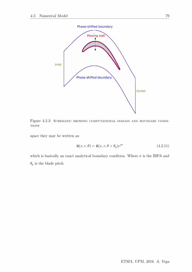
4.2. Numerical Model 79
Phase-shifted boundary
Inlet
Outlet
Phase-shifted boundary
Figure 4.2.3: Schematic showing computational domain and boundary condi-tions
space they may be written as:
u(x, r, θ) = u(x, r, θ + θp)ejσ (4.2.11)
which is basically an exact analytical boundary condition. Where σ is the IBPA and
θp is the blade pitch.
ETSIA, UPM, 2016. A. Vega


Chapter 5
Low Reduced Frequency Limit
Analysis
There is nothing so practical as a
good theory
James Clerk Maxwell
Contents
5.1 State of the Art . . . . . . . . . . . . . . . . . . . . . . . . 81
5.2 Asymptotic Analysis at Low Reduced Frequency . . . . 82
5.3 Calculus of the Unsteady Loading Parameter . . . . . . . 92
5.4 Simplified Analytical Model for the Work-per-cycle . . . 100
5.5 Review of Theodorsen’s Theory . . . . . . . . . . . . . . . 105
5.6 Conclussions of the Analysis at Low Reduced Frequency 109
5.1 State of the Art
After many years of research, there are three well known parameters correlated to
LPT flutter, that are commonly considered when designing LPT blades: the reduced
81

82 Chapter 5. Low Reduced Frequency Limit Analysis
frequency [6], the steady conditions, and the vibration mode-shape [89, 5]. Panovsky
and Kielb [90], created a preliminary design tool for LPT blades, the Tye-Dye (TD)
plots, which combined the interdependency of critical reduced frequency (the limit
at which the configuration is stable) with vibration mode shape all in a single plot.
There are a number of well know trends of the work-per-cycle curves related with the
aforementioned parameters that are commonly acepted and have been proved several
times. Among this widely known trends it can be mentioned: the stabilizacion of the
work per cycle curves with the reduced frequency, and the differences observed in the
shape of the work per cycle curves when considering different vibration mode-shapes.
An example of the second trend is that flap modes (and usually torsion modes) are
much more unstable than the edge modes [5, 1].
All this facts are based on experience, and there is a lack of sound theoretical support,
and/or physical understanding of the basic mechanisms which govern the behavior of
the work per cycle curves (which in turn represents the stability of a configuration)
with the reduced frequency and the mode-shape.
As a consecuence, in recent years, there is a renewed interest in understanding
the fundamentals of the aerodynamics of oscillating airfoils, and several authors
[91, 92, 93, 94, 95, 96] have made strong efforts to throw some light in the subject;
especially in the context of turbine flutter, which is considered the simplest flutter
instability of all.
5.2 Asymptotic Analysis at Low Reduced Frequency
5.2.1 Governing Equations
The time-dependent Navier-Stokes equations of an ideal gas in conservative and
compact form can be written as:
∂U
∂t+∇.Fc(U) = ∇.Fv(U) (5.2.1)
ETSIA, UPM, 2016. A. Vega

5.2. Asymptotic Analysis at Low Reduced Frequency 83
where U = ρ, ρv, ρET is the vector of conservative variables and Fc and Fv
are the convective and viscous fluxes respectively. Without loss of generality the
simplest boundary conditions for a two-dimensional airfoil cascade could be written
as: Pt = P0, Tt = T0 and α = αin at the inlet; p = pexit at the exit, null velocity,
v = 0, and heat flux, ∂T/∂n = 0, are prescribed at the airfoil’s solid walls whereas
periodic boundary conditions are enforced at the lateral boundaries of the airfoil
passage.
The above equations may be non-dimensionalised using pc = P0, Tc = T0 and
v2c = 2cpT0(1 − (pexit/P0)(γ−1)/γ) as the characteristic pressure, temperature and
velocity respectively. The characteristic velocity used here is the isentropic exit
velocity that may be readily computed from the boundary conditions. The airfoil
chord, c, is used as the characteristic length, Lc. Then, choosing the inverse of ω as
the characteristic time, tc = ω−1, Eq. 5.2.1 can be written in non-dimensional form
as:
k∂U
∂τ= −∇.Fc(U) +
1
Re∇.Fv(U) = −∇.F(U) (5.2.2)
where τ = ωt is the non-dimensional time, x = x/c the non-dimensional distance
and U = ρ, ρW, ρET the vector of non-dimensional conservative variables, with
ρ = ρ/ρ0, p = p/P0 W = v/vc and E = 12γT /(1 − Π
−(γ−1)/γR ) + 1
2W
2. The non-
dimensional boundary conditions become Pt = 1, Tt = 1 and α = αin at the inlet
and p = Π−1R at the exit where ΠR = P0/pexit is the pressure ratio of the row or the
cascade. The non-dimensional solution of the problem, for a given geometry, depends
on:
U = f(x, τ,ΠRRe, k, γ, ) (5.2.3)
where Re is the Reynolds number based on the characteristic velocity and the chord,
and k is the so-called reduced frequency:
k =ωc
vc(5.2.4)
which represents the ratio between the flow-through time and the characteristic time
of the motion, or the inverse of the frequency if the motion is harmonic.
ETSIA, UPM, 2016. A. Vega
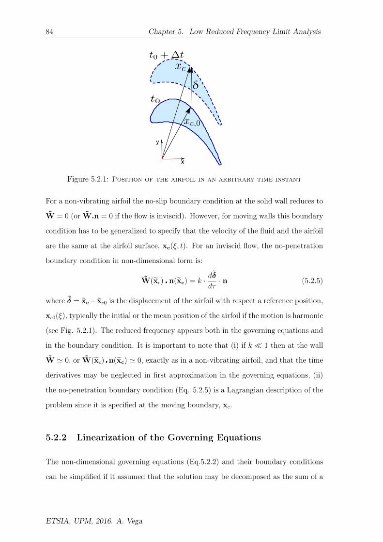
84 Chapter 5. Low Reduced Frequency Limit Analysis
x
y
Figure 5.2.1: Position of the airfoil in an arbitrary time instant
For a non-vibrating airfoil the no-slip boundary condition at the solid wall reduces to
W = 0 (or W.n = 0 if the flow is inviscid). However, for moving walls this boundary
condition has to be generalized to specify that the velocity of the fluid and the airfoil
are the same at the airfoil surface, xc(ξ, t). For an inviscid flow, the no-penetration
boundary condition in non-dimensional form is:
W(xc) n(xc) = k · dδdτ· n (5.2.5)
where δ = xc− xc0 is the displacement of the airfoil with respect a reference position,
xc0(ξ), typically the initial or the mean position of the airfoil if the motion is harmonic
(see Fig. 5.2.1). The reduced frequency appears both in the governing equations and
in the boundary condition. It is important to note that (i) if k 1 then at the wall
W ' 0, or W(xc) n(xc) ' 0, exactly as in a non-vibrating airfoil, and that the time
derivatives may be neglected in first approximation in the governing equations, (ii)
the no-penetration boundary condition (Eq. 5.2.5) is a Lagrangian description of the
problem since it is specified at the moving boundary, xc.
5.2.2 Linearization of the Governing Equations
The non-dimensional governing equations (Eq.5.2.2) and their boundary conditions
can be simplified if it assumed that the solution may be decomposed as the sum of a
ETSIA, UPM, 2016. A. Vega

5.2. Asymptotic Analysis at Low Reduced Frequency 85
mean baseline flow, U0(x), plus a small unsteady perturbation, u(x, τ):
U(x, τ) = U0(x) + u(x, τ) (5.2.6)
such that u U0. It may be shown that this approximation is valid if the vibration
amplitude, ‖δ‖, is much smaller than the airfoil’s chord, i.e.: ‖δ‖ c, and highly
non-linear phenomena, such as shock-waves and separation bubbles, are not present
in the mean flow-field. Under these hypotheses the Navier-Stokes equations may be
linearized about the mean flow to yield:
k∂u
∂τ+
∂
∂x
(A0(U0)u
)= 0 (5.2.7)
where A0 = (∂F/∂U)0 is the non-dimensional Jacobian matrix, and U0 satisfies
∇.F(U0) = 0. The linearization of the wall boundary conditions deserves special
attention and it is addressed in the following sub-section.
5.2.3 Linearization of the no-penetration boundary condition
It has been previously mentioned than the airfoil’s no-slip boundary condition
(Eq. 5.2.5) is expressed in Lagrangian form because it is imposed in a moving
boundary. Linearized Navier-Stokes codes designed to deal with vibrating airfoils
usually implement the no-slip boundary condition, and the rest of the algorithm,
in a fixed grid, but implicitly compute the forcing terms in a moving grid. Non-
linear codes implement the whole algorithm in moving grids, and the wall boundary
condition is implemented exactly as specified in Eq. 5.2.5 (see for instance [75, 32]).
However for analytical studies this form hides relevant information. When k 1,
the condition reduces to W ' 0 at x = xc(τ), concealing the fact that there is a
quasi-steady displacement of the airfoil that makes the airfoil loading change with
time. This trivial observation is not easy to explicitly state from a mathematical
point of view within this formulation.
Alternatively, the no-penetration boundary condition may be linearized and explicitly
expressed in Eulerian form in the same way that was done by Verdon [42] in the
resolution of the transonic unsteady potential equation. The non-dimensional fluid
ETSIA, UPM, 2016. A. Vega
86 Chapter 5. Low Reduced Frequency Limit Analysis
velocity field may be expressed as:
W(x, τ) = W0(x) + w(x, τ) (5.2.8)
where W0(x) represents the mean velocity and w(x, τ) the perturbed velocity, with
w W0. The no-penetration boundary condition can then be written as:
[W0(xc0 + δ) + w(xc0 + δ, τ)] · [n(xc0) + (δ · ∇)n] = k · dδdτ· n (5.2.9)
where, the term (δ ∇)n, which accounts for the variation of the normal direction of
the airfoil due to the rotation of the airfoil in the mean flow field, has been retained.
This term does not explicitly appear in the linearization of the no-slip boundary
condition, since in this case the normal to the airfoil is not involved in the boundary
condition.
The boundary condition on the actual position of the airfoil may be referred to its
mean or initial position, xc0. Assuming that∥∥∥δ∥∥∥ 1, expanding W in Taylor
series, neglecting second-order terms, and recalling that W0(xc0).n = 0, the previous
equation reduces to:
(δ ∇)W0
∥∥∥x=xc0
· n(xc0) + w(xc0) · n + W0(xc0) · (δ · ∇)n = k · dδdτ· n
and the no-penetration linearized boundary condition becomes:
w(xc0).n = k · dδdτ.n− (δ · ∇)W0
∥∥∥x=xc0
.n− W0(xc0) · (δ · ∇)n (5.2.10)
The important fact is that this boundary condition is imposed in the original
undeformed airfoil and physically represents a blowing velocity in the wall boundary.
Numerical codes that implement this type of boundary condition do not need to
resort to the use of moving grids because they implicitly assume that the airfoil
displacements are small. The boundary condition now provides a new term, that was
hidden when expressing it in Lagrangian form. This term is what has been called the
Unsteady Loading Parameter (ULP), and it represents a new aeroelastic parameter.
It can be clearly seen that the term W0(xc0) · (δ · ∇)n vanishes for a pure bending
mode, since in this case ∇n = 0 during the airfoil motion. In others words, this
term is only important for torsion modes, especially, as it will be shown later on, for
ETSIA, UPM, 2016. A. Vega
5.2. Asymptotic Analysis at Low Reduced Frequency 87
lightly loaded airfoils or plates vibrating in torsion at low reduced frequency, where
it becomes the leading term in Eq. 5.2.10, since in this case ∇W0 ' 0.
For rigid blade motions:
δ = h+α× r (5.2.11)
where h defines the amplitude and direction of blade translations, α is the angle
(positive counter clockwise) of blade rotation, and r is the position vector extending
from the axis of rotation to the mean position of the airfoil surface. In this case, the
linearized no-penetration boundary condition reduces to:
w(xc0).n =
[k · dδ
dτ− (δ · ∇)W0
∥∥∥x=xc0
+α× W0(xc0)
]· n (5.2.12)
where it is more clearly seen that the third term in the r.h.s. is related with the
rotation of the airfoil.
The fact that the rotational term appears only explicitly in the inviscid no-penetration
boundary condition does not mean that its effect is not present in viscous flows
provided that there is no separation. If the flow remains attached to the airfoil
the flow-field can be decomposed in a thin boundary layer close to the airfoil and
an external inviscid flow. The boundary conditions for this external flow-field are
identical to that of an inviscid case with an additional, steady transpiration velocity
at the wall to account for the boundary layer thickness [97, 98].
5.2.4 Asymptotic Analysis of the Linearized Equations
Although perturbation methods areimplicitly used in the derivation of the linearized
governing equations, with few exceptions they have not been used to seek simplified
solutions of the Euler or Navier-Stokes equations in the presence of moving walls.
Moore [7] used an asymptotic analysis to derive a quasi-analytical solution for an
axially oscillating flat plate with a laminar boundary layer, in the low-reduced
frequency limit. Interestingly, it may be anticipated that the mathematical structure
of the solution that he obtained, is exactly the same as that it has been found in this
thesis, since the oscillating flat plate is just particular case of a more generic class of
ETSIA, UPM, 2016. A. Vega

88 Chapter 5. Low Reduced Frequency Limit Analysis
problems described here.
Different levels of approximation of the linearized Navier-Stokes equations may be
obtained taking advantage of the smallness of k, and assuming that the displacement
of the airfoil and the flow are periodic in time, i.e.: δ = δeiωt and u = ueiωt. For the
sake of simplicity in the notation from now on, within this section, unless explicitily
mentioned otherwise, the term − ∇W0
∥∥∥x=xc0
δ will be used instead of the full
expression when referring to the Unsteady Loading Parameter,Υ, which means that
the whole term Υ = −(δ · ∇)W0
∥∥∥x=xc0
+ α × W0(xc0) is substituted by a more
compact expression.
5.2.4.1 0th Order Approximation
If it is assumed that k = 0 the linearized system of equations reduces to:
∂
∂x
(A0(U0)u0
)= 0, with w0(xc0).n = − ∇W0
∥∥∥x=xc0
δ.n (5.2.13)
where the characteristic amplitude of u0 is of order uc ∼∥∥∥δ∥∥∥, which is small if
∇W0
∥∥∥x=xc0
∼ o(1). The pressure and the rest of the variables are in-phase with
the displacement, since physically they are due to the perturbation of the base flow
associated to the static displacement of the airfoil. In this approximation, time plays
the role of a parameter. For a harmonic motion whose solution may be expressed in
the complex domain, the solution is real and the phase of the solution with the airfoil
displacement, φ0 = 0.
5.2.4.2 1st Order Approximation
The first order correction of the solution with k may be obtained if the velocity is
expressed as:
u(x, τ) = u0(x, τ) + u1(x, τ) (5.2.14)
Introducing the above expression in Eqs 5.2.7 and 5.2.10, the 1st order correction
for the governing equations and the boundary condition in the frequency domain is
ETSIA, UPM, 2016. A. Vega

5.2. Asymptotic Analysis at Low Reduced Frequency 89
obtained:
iku0 +∂
∂x
(A0(U0)u1
)= 0, with w1(xc0) = ikδ (5.2.15)
where for the sake of simplicity the tilde to indicate non-dimensional variables has
been omitted, and awe have ssumed that the motion is harmonic in time, and the
displacement has only a real component, δ = δR, i.e.: it is the origin of the phases and
a real mode is being considered. In this case u1 is purely imaginary, u1 = u1I +h.o.t.,
since u0 is real. The characteristic value of the correction u1c ∼ k ‖δ‖ is much smaller
than the characteristic value of the zero order approximation u0c ∼ ∇W0c ‖δ‖, since
k 1. The 1st order correction of the phase, φ1, may be estimated as:
tanφ1 ∼u1Ic
u0c
∼ k(1 + α∗∇W0c)
∇W0c
(5.2.16)
which is small as well, since k 1 and α∗ is a constant of order one, actually φ1 ∝ k
if ∇W0c ∼ o(1), exactly as it will be seen in the numerical validation chapter.
5.2.4.3 2nd Order Approximation
The next approximation of the solution provides the correction with the frequency of
the real part of the solution. As it will become apparent in the following section, this
correction provides further insight of the solution for lightly loaded airfoils, of which
the flat plate is the limiting case. When the gradient of the velocity of the mean flow
vanishes, the quasi-steady motion of the airfoil does not cause any perturbation and
the next approximation of the flow is needed.
Following a consistent perturbation analysis, the 2nd order approximation is given by:
−ku1I +∂
∂x
(A0(U0)u1R
)= 0, with w1R(xc0) = 0 (5.2.17)
where it has been assumed that u1 = u1R+iu1I and that u1I is already known from
the previous expansion. It can be observed that the time derivative is responsible
of coupling the real and imaginary parts of the solution. The characteristic value of
u1R is, according with the previous equation, u1Rc ∼ ku1Ic ∼ k2 ‖δ‖. The 2nd order
ETSIA, UPM, 2016. A. Vega

90 Chapter 5. Low Reduced Frequency Limit Analysis
approximation of the phase, φ2, is then:
tanφ2 ∼u1Ic
u0c + u1Rc
∼ k
a∇W0c + bk2(5.2.18)
where a and b are real constants of order unity. It may be readily observed that for
highly loaded airfoils (i.e.: ∇W0c ∼ o(1)), if k 1 then φ ∼ k; which is one of the
first conclusions of the analysis. However, for lightly loaded airfoils (i.e.: ∇W0c ' 0),
φ ' π/2 − dk even if k 1 (d is as well a real constant of order unity). This is a
second major conclusion.
5.2.5 Estimate of the Unsteady Pressure
For highly loaded airfoils the leading term of the previous expansion is u0, which is
real and in phase with the displacement, being its characteristic value uc0 ∼∥∥∥δ∥∥∥Υ.
Since p = p/P0 and p varies from 1 at the inlet to Π−1R at the exit, the characteristic
unsteady pressure is:
p′c0 ∼1
2ρcv
2c
(δcc
)Υ (5.2.19)
since the perturbation of the flow is purely static and, therefore, the unsteady pressure
is proportional to the dynamic head and the displacement.
Its first order correction with k is due to the airfoil vibration velocity and is associated
to u1, whose characteristic value is u1c ∼ k ‖δ‖, and therefore the correction of the
pressure perturbation due to the unsteady terms is of the order of
p′c0 ∼1
2ρcv
2c
(δcc
)(ωc
vc
)∼ ρcvcωδc. (5.2.20)
This second scaling is only relevant if either the unsteady aerodynamic loading is low
or vanishes. Strictly speaking this is the order of the unsteady pressure when Υ k.
This means that even for low reduced frequencies, i.e.: k 1, if the unsteady loading
parameter is small enough, the value of the characteristic pressure is given by 5.2.20.
This scaling is also valid for reduced frequencies of order unity (i.e.: k ∼ 1), since in
this case Eqs. 5.2.19 and 5.2.20 are equivalent.
ETSIA, UPM, 2016. A. Vega
5.2. Asymptotic Analysis at Low Reduced Frequency 91
5.2.6 Summary
According with the previous perturbation analysis, some conclusions may be drawn
for vibrating airfoils at low reduced frequency. In this context low means much
smaller than one. From a mathematical point of view it is necessary to have k ∼ 0.1
to formally support the analysis although, as it will be shown in the numerical
validation chapter, the conclusions hold as well for higher values of k, being the actual
threshold, for which the current analysis is valid, case dependent. Flutter boundaries
for cantilever LPTs are in the range of k ∼ 0.1 − 0.2 [1] and, as a consequence, the
following conclusions may be applied to realistic aeroelastic configurations:
1. The influence coefficient phase of highly loaded airfoils, i.e. Υ ∼ o(1), changes
linearly with k, i,e,: φ ∝ k 1, and therefore is small. The unsteady pressure
induced by the vibration is given by Eq. 5.2.19 and therefore the influence
coefficients are in first approximation independent of k and proportional to the
dynamic head and the unsteady loading parameter. The influence coefficient of
the j-th airfoil, lj, can be written as:
lj =1
2ρcv
2c
(δcc
)Υ c
(l0j + l1j
k
Υ
)(5.2.21)
if the dependence with k is retained. This means that in second order
approximation the influence coefficient varies linearly with k.
2. The phase of lightly loaded airfoils, i.e. when Υ ' 0 or more precisely Υ k,
departs from π/2 and varies linearly with k, i.e.: φ − π/2 ∝ k. This fact has
a deep impact on the work-per-cycle curves as it will be shown later on. The
unsteady pressure induced by the vibration is given in this case by Eq. 5.2.20
and hence the influence coefficients scale with k for lightly loaded airfoils and
can be written as:
lj = ρcvcωδcc l0j (5.2.22)
that can be seen as the limit of Eq. 5.2.21 when Υ→ 0.
ETSIA, UPM, 2016. A. Vega

92 Chapter 5. Low Reduced Frequency Limit Analysis
5.3 Calculus of the Unsteady Loading Parameter
5.3.1 Integral Unsteady Loading Parameter
The order of magnitude of the second and third terms in the r.h.s. of Eq.5.2.12 can
be estimated if the mean flow-field is known. The second term is directly related
with the steady loading of the airfoil, and is typically of order unity since usually the
velocity changes of the order of itself in distances of the order of the chord. The third
term is also of order unity since the velocity has been non-dimensionalized with the
exit velocity.
However, both ∇W0 and W0, are point-wise variables since they change along the
airfoil chord. In order to quantitatively predict the effect of the unsteady loading in
the work-per-cycle curves, the Unsteady Loading Parameter (ULP) has been defined
as:
Υ =1
2δmax
˛ρW2
0(δ · ∇)W0 · nds+
˛αρW3
0ds
(5.3.1)
where the integrals extend along the whole airfoil surface, δmax is the maximum of
the non-dimensional displacements, and ds is the non-dimensional arc-length. The
first term of the r.h.s. represents the loading contribution, ULPL, while the second
term is the rotational contribution, ULPR, which is zero for bending modes and a
constant contribution for any torsion mode, independently of its torsion center.
It may be noticed that both contributions are weighted with the local non-dimensional
dynamic pressure, 12ρW2
0(s), since the unsteady pressure associated to the airfoil
vibration and the work-per-cycle are proportional to the dynamic head. Therefore,
the ULP accounts for the fact that the unsteady pressure generated in the vicinity
of the stagnation point is much smaller than that created in the suction side of the
airfoil, where the peak Mach number is usually attained at design conditions.
Moreover, the ULP is mode dependent since δ(s) depends on the actual mode-shape.
The beauty of the ULP is that it is able, as it will be shown later on, to account for
the effect of the mode-shape and the aerodynamic loading distribution, in the low
reduced frequency limit, without performing any unsteady simulation.
ETSIA, UPM, 2016. A. Vega

5.3. Calculus of the Unsteady Loading Parameter 93
The loading contribution to the ULP may be obtained in practice as:
ΥL =
˛1
2δmaxρW2
0∂W0
∂n· δnds (5.3.2)
where δn is the airfoil displacement in the normal direction.
In order to calculate the integral Unsteady Loading Parameter for viscous cases, it
is enough to substitute in Eq. 5.3.1 the velocity at the airfoil surface, W0, that
is actually zero for a viscous case, by the isentropic velocity at the airfoil surface.
In this thesis, for the sake of simplicity , inviscid cases are mostly considered, but
the influence coefficient modulus and phase of the unsteady pressure, as well as
the work-per-cycle curves, of vibrating airfoils do not considerably differ between
viscous and inviscid cases, provided that the flow remains attached to the airfoil.
Figure 5.3.1 displays the non-dimensional work per cycle curves as a function of the
IBPA for an LPT airfoil vibrating in flap mode at design conditions for a reduced
frequency k = 0.1. It can be seen that the impact of viscous effects is very small
for classical flutter. Obviously there are aeromechanic instabilities that are driven
by viscous effects, such as stall flutter [18], and in this case the conclusions would
have to be revisited, but it will be shown that the ULP derived in the present thesis
is strongly correlated with the unsteady aerodynamics of oscillating airfoils at low
reduced frequency provided that the flow remains attached to the airfoil.
5.3.2 Interpretation of the Unsteady Loading Parameter
Let us consider the momentum equation of a steady inviscid flow:
ρV.∇V = −∇p (5.3.3)
If the previous equation is expressed in its components along the streamline direction,
t, and its normal, n, it is obtained that :
t : ρV∂V
∂s= −∂p
∂s
n : ρV 2
R=
∂p
∂n
(5.3.4)
ETSIA, UPM, 2016. A. Vega

94 Chapter 5. Low Reduced Frequency Limit Analysis
−180 −135 −90 −45 0 45 90 135 180
IBPA
−2
−1
0
1
2
Θ=
Wcycle/(
πρ
cU
c
2δ
c
2/2
)
Inviscid case
Viscous case
Figure 5.3.1: Non-dimensional damping as a function of the IBPA for the LPTcase vibrating in flap (M = 0.74, k = 0.1) for a viscous and an inviscid case.
In the incompressible limit, ρ = ρ0, the momentum equation along the streamlines
reduces to the Bernoulli equation:
P0 = p+1
2ρ0V
2 (5.3.5)
where P0 is the stagnation pressure of that streamline. If the flow is homeotropic and
all the streamlines have the same stagnation pressure, Eq. 5.3.5 may be injected in
the normal component of the momentum equation (5.3.4) to obtain:
1
V
∂V
∂n= − 1
R(5.3.6)
where R is the local radius of curvature of the streamline. For an attached flow, the
airfoil is a streamline and, therefore, the tangent and normal of the streamline are
indistinguishable from those of the airfoil. This means that: ∇W0 · n ' W0/R.
A similar result may be obtained for compressible flows using the isentropic condition.
In this case, it may be shown that:
1
M
dM
dn= − 1
R
(1 +
γ − 1
2M2
)−1
(5.3.7)
which is the compressible counter part of Eq.5.3.6. A similar expression to 5.3.6 can
ETSIA, UPM, 2016. A. Vega

5.3. Calculus of the Unsteady Loading Parameter 95
be obtained for the compressible case realizing that:
1
V
∂V
∂n=
1
Ma
d(Ma)
dn=
1
M
dM
dn+
1
a
da
dn(5.3.8)
where a is the sound speed and a0 the stagnation sound speed. Taking into account
thata0
a=(1 + γ−1
2M2)1/2
= Γ1/2, the second term of the right hand side can be
written as:
1
a
∂a
∂n= −1
2(γ − 1)Γ −1M
dM
dn(5.3.9)
and then:
1
V
∂V
∂n=
1
M
dM
dn
[1− γ − 1
2ΓM2
]= − 1
R
[Γ−1 − γ − 1
2Γ−2M2
](5.3.10)
If is considered M = 0.7, then γ−12M2 ' 0.1 1, and then:
1
V
∂V
∂n' − 1
R
[1− γ − 1
2M2
]= − 1
R(1− ε), (5.3.11)
where the error, ε, with respect the expression 5.3.6, is ε < 10%, if M < 0.7.
If the displacements induced by bending and torsion are comparable, i.e.: δ ∼ α,
the ratio between the loading and rotational contributions is the radius of curvature.
Actually, ∇nW could be estimated as: ∇nW ' W/R.
5.3.3 Examples
With the aim of illustrating the meaning of the different components of the ULP,
an LPT airfoil (see Fig. 5.3.2), which will be described in detail in the numerical
validation chapter, has been selected. The design operating point is defined by an
inlet and exit angle of α1 = 44 and α2 = 60, respectively, exit Mach number of
Mexit = 0.75 and a pitch to chord ratio of s/c = 0.96.
Figure 5.3.3 displays the distribution along the airfoil of the normal gradient of
the velocity divided by the velocity, computed using three different approaches:
(i) computing the flow-field velocity gradient in the normal projection into the
airfoil, which is considered as the exact method ( symbols) (ii) the incompressible
approximation, i.e.: the inverse of the non-dimensional radius of curvature, 1/R =
ETSIA, UPM, 2016. A. Vega

96 Chapter 5. Low Reduced Frequency Limit Analysis
-1
0
+1
Figure 5.3.2: Snapshot of the unsteady pressure caused by the vibration ofthe central blade in an LPT airfoil for k = 0.3.
0 0.25 0.5 0.75 1
x/c
−4
−2
0
2
4
(dV
/dn
)/V
1/R F(M)
Exact Method
1/R
Pressure Side
Suction Side
Figure 5.3.3: Distribution of the normal gradient of the velocity alongan LPT airfoil computed using three different approaches
ETSIA, UPM, 2016. A. Vega

5.3. Calculus of the Unsteady Loading Parameter 97
0 0.25 0.5 0.75 1
x/cx
−2
0
2
4
6
UL
P C
on
trib
uti
on
s
ULPL LE Torsion
ULPR
ULPL Flap
Figure 5.3.4: Unsteady loading parameter distribution (loading contribution,ULPL,and rotational contribution, ULPR) along an LPT airfoil for differ-ent mode-shapes.
cax/R , (M symbols) and (iii) the compressible correction to 1/R, i.e.: 5.3.8, (N
symbols). First of all, it may be noticed that the distribution of the normal gradient
of the velocity along the airfoil resembles the distribution of 1/R, confirming the
physical interpretation outlined in the preceding sub-section. Moreover, large peaks
can be seen both, in the leading and trailing edges caused by the small radius of
curvature of the l.e. and t.e., that give rise to very large local velocity gradients.
These peaks are not only undesirable, but have low physical sensitivity, since they
occur in regions of low velocity, that generate very low levels of unsteady pressure.
For this reason, the forcing terms generated in the wall no-penetration boundary
condition (Eq. 5.2.12), and that form the core of the ULP integrand, are weighted
with the local dynamic head to properly scale its impact on the final result.
Figure 5.3.4 depicts the ULP distribution for the same airfoil for two modes: flap and
torsion about the l.e. The peak of the ULP for the flap mode is close to the location of
the maximum unsteady pressure modulus, as it can be seen in Fig. 5.3.2, which shows
the unsteady pressure modulus for the LPT configuration under study, vibrating in
flap mode at a reduced frequency k = 0.3; obviously the rotational contribution to the
ULP is zero for this case. It can be seen that the ULP distribution is able to predict
ETSIA, UPM, 2016. A. Vega

98 Chapter 5. Low Reduced Frequency Limit Analysis
0 0.5 1
x/cx
0
0.5
1
1.5
2
Mis
LPT (Mexit
=0.75)
NACA 65 (Min =0.7)
NACA 65 (Min =0.8)
Figure 5.3.5: Isentropic mach number distributions along the airfoil chordfor the LPT and the NACA65 cases
where will be located the maximum of the unsteady pressure, which constitutes a
very surprising result since, the ULP has been obtained only from the steady flow
field and the given vibration mode shape, without using any unsteady data. The
maximum of the loading contribution to the ULP for a torsion mode about the l.e.
occurs downstream of the peak of the flap mode, since the local vibration amplitude
increases with the axial length in this case, causing a downstream shift with respect
the peak of the previous case. The rotational component of the ULP parameter is
fairly constant along the chord, but lower than the loading contribution. The ratio
between both, the loading and rotational contributions is consistent with Eq. 5.3.8
that predicts a factor of 1/R, that in this case is roughly 3 (see Fig. 5.3.3).
The contribution of the suction side is much larger than that of the pressure side,
by a factor of about 100. This is consistent with the fact that the isentropic velocity
in the suction side is about five times greater than in the pressure side (see the zero
incidence isentropic Mach number distribution in Fig. 5.3.5), and that the integrand
of the ULP scales with the cube of the non-dimensional velocity. The accumulated
contribution to the ULP can be also seen in Fig, 5.3.6 (♦). It can be noticed that the
contribution increases smoothly along the chord, and that the influence of the l.e. is
negligible, except by a small contribution to the p.s. that gives rise to a small off-set
ETSIA, UPM, 2016. A. Vega
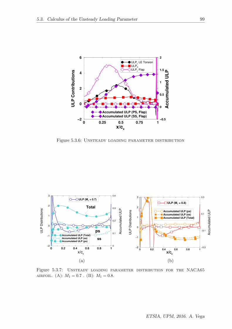
5.3. Calculus of the Unsteady Loading Parameter 99
0 0.25 0.5 0.75 1−2
0
2
4
6
UL
P C
on
trib
uti
on
s
ULPL LE Torsion
ULPR
ULPL Flap
x/cx
−0.5
0
0.5
1
1.5
2
Accu
mu
late
d U
LP
Accumulated ULP (PS, Flap)
Accumulated ULP (SS, Flap)
Figure 5.3.6: Unsteady loading parameter distribution
0 0.2 0.4 0.6 0.8 1−2
−1
0
1
2
3
UL
P D
istr
ibu
tio
ns
ULP (M1 = 0.7)
0 0.2 0.4 0.6 0.8 1
x/cx
0
0.1
0.2
0.3
0.4
Accu
mu
late
d U
LP
Accumulated ULP (Total)
Accumulated ULP (ss)
Accumulated ULP (ps)
ps
ss
Total
0 0.2 0.4 0.6 0.8 1
x/cx
−2
−1
0
1
2
3
UL
P D
istr
ibu
tio
ns
ULP (M1 = 0.8)
0 0.2 0.4 0.6 0.8 1
x/cx
−0.3
−0.1
0.1
0.3
Accu
mu
late
d U
LPAccumulated ULP (ps)
Accumulated ULP (ss)
Accumulated ULP (Total)
(a) (b)
Figure 5.3.7: Unsteady loading parameter distribution for the NACA65airfoil. (A): M1 = 0.7 . (B): M1 = 0.8.
ETSIA, UPM, 2016. A. Vega

100 Chapter 5. Low Reduced Frequency Limit Analysis
respect to zero.
Figure 5.3.7 displays the ULP distribution for the NACA65 airfoil operating at
subsonic (left) and transonic (right) conditions, for the flap mode. The subsonic
operating point (see [9, 99]) is defined by an inlet angle α1 = 55ş , exit angle α2 = 40ş,
inlet and exit isentropic Mach number, Min = 0.7 and Mexit = 0.45, respectively, and
airfoil spacing, s/c = 1; and for the transonic case the inlet isentropic Mach number
is raised to Min = 0.8. The isentropic Mach number distributions can be seen in
Figure 6.2.1. When looking at the ULP distributions, it can be seen that, on the
contrary than in the LPT case, the l.e. contribution is very high, actually most
of the ULP is created in this region in both, the subsonic and the transonic cases.
The transonic condition gives rise to a large discontinuity in the region where the
shock wave is sitting on the airfoil (x/c ' 0.2), that nearly balance that created on
the l.e. The contribution to the ULP of the region downstream of the shock-wave
is almost negligible. When looking to Fig. 5.3.8, which represents the imaginary
part of the unsteady pressure for the NACA65 operating at subsonic and transonic
conditions, vibrating in flap mode, at reduced frequency k = 0.1, it can be seen that,
as it happens with the LPT case, the ULP correctly predicts the region where the
maximum of the imaginary part of unsteady pressure, which means the region that
will mostly contribute to the work per-cycle, will be located.
The different behavior of the NACA65 and the LPT airfoils is due to the distinct
distributions and values of the radius of curvature on both airfoils, that is much
higher and sharp in the l.e. region of the compressor airfoil.
5.4 Simplified Analytical Model for the Work-per-
cycle
The previous assertions have direct implications on the shape of the work-per-cycle
curves. It has been previously reported [5, 100], that for LPT airfoils, and in general
for highly loaded subsonic airfoils, vibrating in flap and edge-wise modes, only the
ETSIA, UPM, 2016. A. Vega

5.4. Simplified Analytical Model for the Work-per-cycle 101
(a) (b)
Figure 5.3.8: Imaginary part of the unsteady pressure of the NACA65Compressor for k = 0.1, for Min = 0.7 (a) and for Min = 0.8 (b)
ETSIA, UPM, 2016. A. Vega

102 Chapter 5. Low Reduced Frequency Limit Analysis
vibrating airfoil, j = 0, and the adjacent airfoils, j = ±1, contribute significantly to
the work-per-cycle, Wcycle. The same assumption has been adopted here. It may be
shown that the work-per-cycle can be expressed as a function of the inter-blade phase
angle, σ, and the influence coefficients in the following form:
Wcycle = πp′cδcc[l0 sinφ0 + l+1 sin(φ1 − σ) + l−1 sin(φ−1 + σ)
](5.4.1)
where lj and φj are respectively the modulus and phase of the non-dimensional ICs,
and δc the vibration amplitude.
5.4.1 Loaded Airfoils
Taking into account that the phase of the ICs of highly loaded airfoils (Υ ∼ o(1)) is
small and reduces with the unsteady loading:
tanφ ' φ ∼ k(1 + α∗Υ)
Υ(5.4.2)
where α∗ is a constant,
for unsteady loaded airfoils vibrating at k 1 the scaling of Wcycle is as follows:
Wcycle = C[l0φ0 + l±1 sin(φ±1 ∓ σ)
]= C
[l0α0
k(1 + α∗Υ)
Υ+ l±1 sin(α±1φ∓σ)
](5.4.3)
where C = 12πρcv
2cδ
2cΥ. Since φ0 ' α′0k and φ±1 ' α′±1k, where α′0 and α′±1 are
constants of order unity, and the non-dimensional IC moduli, l0 and l±1, are constant
with a small correction proportional to k, then the mean value of the work-per-
cycle, Wcycle−mean, scales with k whereas the variation with σ is constant in first
approximation, i.e.:
Wcycle = Wcycle−mean +W ′cycle(σ, k) = k W 0
cycle +W ′cycle(σ, k) (5.4.4)
where maxk,σW′cycle is bounded with k in first order approximation, as it can be seen
in the numerical results shown in Fig. 5.4.1 for an LPT airfoil vibrating in flap mode.
Numerical experiments have been carried out in the numerical verification chapter,
, to confirm that this is a generic result independent of the geometry. If more ICs
were needed to be retained to accurately represent the solution, as it is sometimes the
ETSIA, UPM, 2016. A. Vega
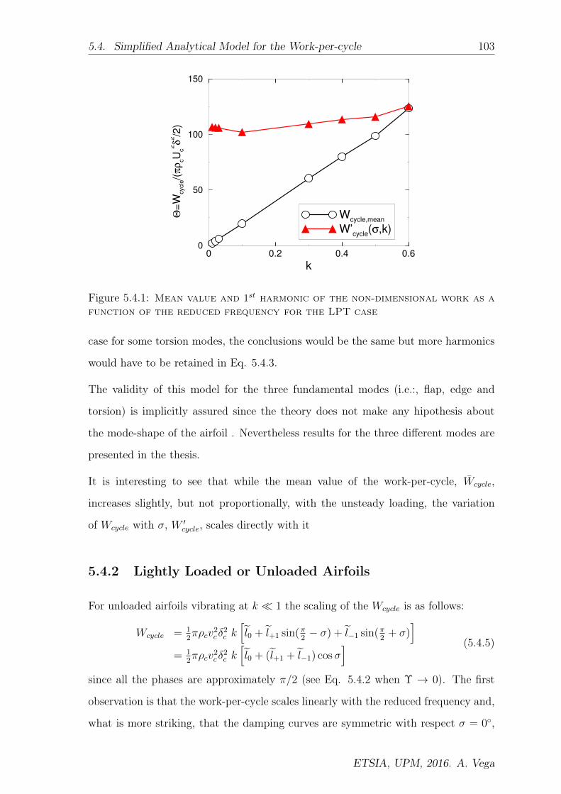
5.4. Simplified Analytical Model for the Work-per-cycle 103
0 0.2 0.4 0.6
k
0
50
100
150
Θ=
Wcycle/(
πρ
cU
c
2δ
2/2
)
Wcycle,mean
W’cycle
(σ,k)
Figure 5.4.1: Mean value and 1st harmonic of the non-dimensional work as afunction of the reduced frequency for the LPT case
case for some torsion modes, the conclusions would be the same but more harmonics
would have to be retained in Eq. 5.4.3.
The validity of this model for the three fundamental modes (i.e.:, flap, edge and
torsion) is implicitly assured since the theory does not make any hipothesis about
the mode-shape of the airfoil . Nevertheless results for the three different modes are
presented in the thesis.
It is interesting to see that while the mean value of the work-per-cycle, Wcycle,
increases slightly, but not proportionally, with the unsteady loading, the variation
of Wcycle with σ, W ′cycle, scales directly with it
5.4.2 Lightly Loaded or Unloaded Airfoils
For unloaded airfoils vibrating at k 1 the scaling of the Wcycle is as follows:
Wcycle = 12πρcv
2cδ
2c k[l0 + l+1 sin(π
2− σ) + l−1 sin(π
2+ σ)
]= 1
2πρcv
2cδ
2c k[l0 + (l+1 + l−1) cosσ
] (5.4.5)
since all the phases are approximately π/2 (see Eq. 5.4.2 when Υ → 0). The first
observation is that the work-per-cycle scales linearly with the reduced frequency and,
what is more striking, that the damping curves are symmetric with respect σ = 0,
ETSIA, UPM, 2016. A. Vega

104 Chapter 5. Low Reduced Frequency Limit Analysis
i.e.:
Wcycle = k W 0cycle(σ) = kW 0
cycle(−σ) (5.4.6)
It is interesting to observe that (i) this symmetry is possible even if l+1 6= l−1 and
(ii) increasing or decreasing the reduced frequency does not produce any noticeable
effect on the stability, i.e.: the sign of Wcyc does not change with k. This behaviour
will be confirmed using numerical experiments. It is important to highlight that for
lightly loaded airfoils it may well happen that more ICs are needed to represent the
mode. It is enough to retain the complete expansion of the Wcycle as a function of
the ICs in Eq. 5.4.5 to conclude that in any case the Wcycle scales linearly with k,
whereas the symmetry with σ may be spoiled if the phase of these ICs is different
from π/2.
5.4.3 Symmetric Cascades
The general form of the Wcycle, Eq. 5.4.1, can be particularized for symmetric
cascades, where l−1 = −l+1 and φ−1 = π + φ+1, in which case Eq. 5.4.1 reduces
to:
Wcycle = πp′cδcc[l0 sinφ0 + 2l+1 sinφ+1 cosσ
](5.4.7)
It has been shown that for loaded airfoils vibrating at k 1, φ ∝ k, while the
influence coefficients are fairly independent of k, (see Eq. 5.2.21) and then:
Wcycle =1
2πρcv
2cδ
2c∇W0c k
[α0l00 + 2α+1l+1 cosσ
](5.4.8)
Two important conclusions can be drawn at this point. The first is that for a
symmetric case the Wcycle curves are symmetric, i.e. Wcycle(σ) = Wcycle(−σ), as
it could be expected because of the symmetry of the problem. The second conclusion
is that the work-per-cycle scales linearly with the reduced frequency for all the inter-
blade phase angles, i.e.:
Wcycle(σ) ∝ k (5.4.9)
ETSIA, UPM, 2016. A. Vega

5.5. Review of Theodorsen’s Theory 105
Since the Wcycle curve of all the unloaded airfoils are symmetric and scale with k,
as well, it can be concluded that all the symmetric cases, for different reasons, fulfill
these two properties.
In the next section, the main aspects of the theory derived by Theodorsen are firstly
presented and finally some conclusions applied to the study of unsteady aerodynamics
in turbomachinery airfoils are directly extracted from the formulation he derived.
5.5 Review of Theodorsen’s Theory
Unsteady aerodynamic theories have been developed for many years for a variety
of uses. The aerodynamics theory developed by Theodorsen, [6], is based on
potential incompressible flow for the lift and pitching moment on an isolated flat
plate oscillating with a frequency ω in a translation in the y direction and in a
rotation about an arbitrary torsion center. The theory assumes small perturbations
and harmonic motion. An analytical solution was obtained for incompressible and
inviscid flow, which gives the loads on the airfoil in terms of the kinematics and
the Theodorsen’s function, that is a function of the reduced frequency, defined as
k = ωc/U∞, where c is the airfoil chord and U∞ the velocity of the free stream.
Theodorsen was able to show that the reduced frequency was the correct measure
of the unsteadiness of the flow because Theodorsen’s function is solely a function of
reduced frequency.
Theodorsen obtained the aerodynamic force as sum of two contributions: the first
is the non circulatory force, determined by a distribution of sources and sinks along
the airfoil surface; and the second is the circulatory force, obtained by superimposing
a vorticity distribution on the body surface (bound vorticity) and in the wake (free
vorticity).
ETSIA, UPM, 2016. A. Vega

106 Chapter 5. Low Reduced Frequency Limit Analysis
x
z
c/2c/2
T.C
h
Figure 5.5.1: Sketch of the displacements of an isolated oscillating plate
5.5.1 Non-circulatory contribution
Theodorsen achieved the solution by distributing sources (upper sides) and sinks
(lower side) of equal strength. According with Theodorsen’s results, the non-
circulatory part of the lift is:
LNC = πc2(h+ U∞α− βcα) (5.5.1)
where c represents the length of the plate, h is the vertical displacement in z direction,
β is the distance between the torsion axis and the origin, and α is the torsion angle.
Figure 5.5.1 represents the plate’s displacement. According with this, a vertical
displacement at constant velocity, h, does not have unsteady effects on the non-
circulatory part of the lift. It is equivalent to the effect of a change in the effective
incidence, α, such that h = Uα.
5.5.2 Circulatory contribution
The non-circulatory part is not able to fulfill the Kutta condition at the trailing edge.
Theodorsen obtained the solution for the circulatory contribution by superimposing
a vorticity distribution on the body surface (bound vorticity) and in the wake (free
ETSIA, UPM, 2016. A. Vega

5.5. Review of Theodorsen’s Theory 107
vorticity). He obtained that the circulatory part of the lift is:
LC = 2πcU∞C(k)
[h+ U∞α + c
(1
2− β
)α
](5.5.2)
where C(k) is the Theodorsen function, that is a function of the reduced frequency.
5.5.3 Conclusions of Theodorsen theory at k 1
The theory derived by Theodorsen can be analized in more detail and some practical
conclussions can be drawn from the expressions he obtained for the lift force. If it is
assumed that the motion of the plate is harmonic in time, then the displacement, h,
and the torsion angle, α, can be expressed as:
h = h0 + ∆h sin(ωt) and α = α0 + ∆α sin(ωt) (5.5.3)
where h0 and α0 represent the mean value and ∆h and ∆α the variations with the
time. The non-circulatory lift can then be written as:
LNC = ρπc2(−∆hω2 sin(ωt) + U∞∆αω cos(ωt) + βc ω2∆α sin(ωt)) (5.5.4)
and in non-dimensional form:
LNC =LNC
12ρU2∞c
= 2π[k2(β∆α−∆h) sin τ + k∆α cos τ
](5.5.5)
where τ = ωt is the non-dimensional time, and ∆h is the non-dimensional
displacement. In a similar way, the circulatory part of the lift can be written as:
LC =1
2ρU2∞4πc
ω
U∞C(k)
[∆h cos(ωt) +
U∞ω
∆α sin(ωt) + (1
2− β) c∆α cos(ωt)
](5.5.6)
which in non-dimensional form is:
LC =LC
12ρU2∞c
= 4π C(k)
[∆α sin τ +
(∆h+
(1
2− β
)∆α
)k cos τ
](5.5.7)
Taking into account the expressions obtained for the non-dimensional lift, and
assuming that k 1 (which directly implies that C(k) ' 1), different order
corrections of the lift with the reduced frequency can be obtained. Table
5.1 summarise the different order corrections to the circulant and non-circulant
ETSIA, UPM, 2016. A. Vega
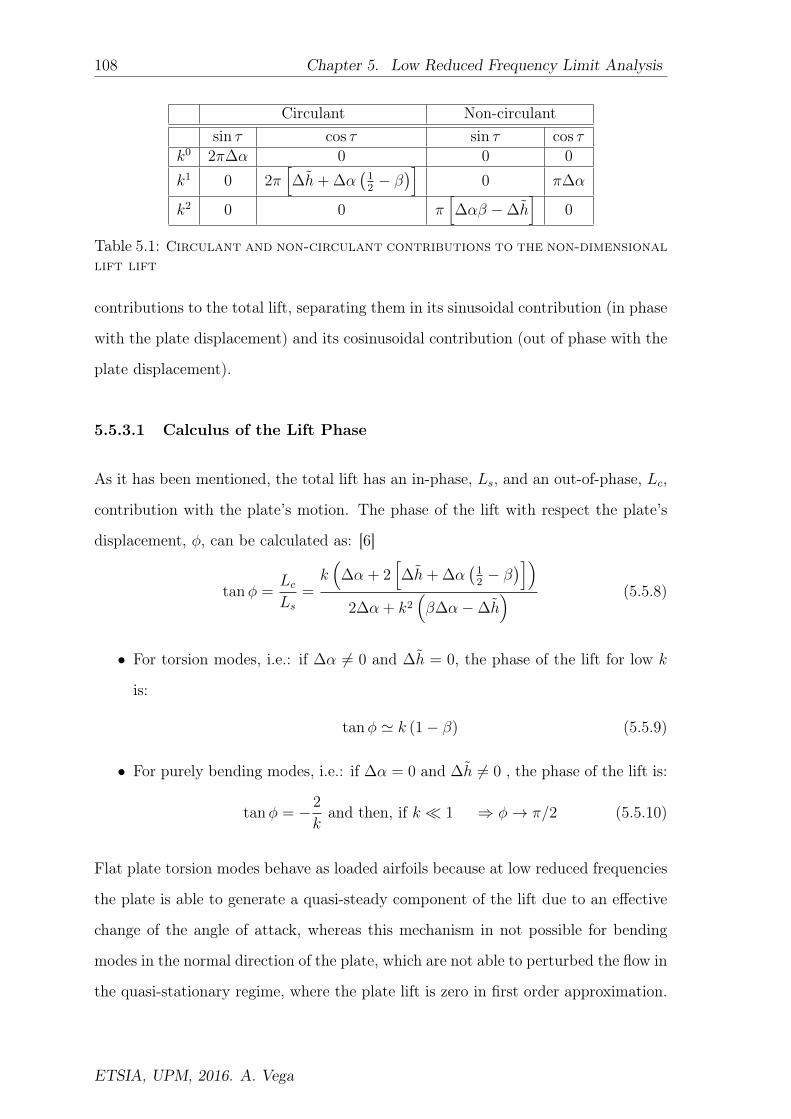
108 Chapter 5. Low Reduced Frequency Limit Analysis
Circulant Non-circulantsin τ cos τ sin τ cos τ
k0 2π∆α 0 0 0k1 0 2π
[∆h+ ∆α
(12− β
)]0 π∆α
k2 0 0 π[∆αβ −∆h
]0
Table 5.1: Circulant and non-circulant contributions to the non-dimensionallift lift
contributions to the total lift, separating them in its sinusoidal contribution (in phase
with the plate displacement) and its cosinusoidal contribution (out of phase with the
plate displacement).
5.5.3.1 Calculus of the Lift Phase
As it has been mentioned, the total lift has an in-phase, Ls, and an out-of-phase, Lc,
contribution with the plate’s motion. The phase of the lift with respect the plate’s
displacement, φ, can be calculated as: [6]
tanφ =LcLs
=k(
∆α + 2[∆h+ ∆α
(12− β
)])2∆α + k2
(β∆α−∆h
) (5.5.8)
• For torsion modes, i.e.: if ∆α 6= 0 and ∆h = 0, the phase of the lift for low k
is:
tanφ ' k (1− β) (5.5.9)
• For purely bending modes, i.e.: if ∆α = 0 and ∆h 6= 0 , the phase of the lift is:
tanφ = −2
kand then, if k 1 ⇒ φ→ π/2 (5.5.10)
Flat plate torsion modes behave as loaded airfoils because at low reduced frequencies
the plate is able to generate a quasi-steady component of the lift due to an effective
change of the angle of attack, whereas this mechanism in not possible for bending
modes in the normal direction of the plate, which are not able to perturbed the flow in
the quasi-stationary regime, where the plate lift is zero in first order approximation.
ETSIA, UPM, 2016. A. Vega
5.6. Conclussions of the Analysis at Low Reduced Frequency 109
Both, the torsion an bending modes, give rise to a in-phase component of the lift,
that that scales with k2, see Table 5.1, and that is not associated to the generation of
circulation. This term, as it was outlined in the previous chapter, 3, is the “apparent”
mass of tthe flat plate and does not generate any damping..
The results obtained from Theodorsen’s theory for the unsteady pressure phase are
the same than that obtained in the asympotic analysis performed in this thesis. It is
important to note that the strong points of the theory presented in this thesis are: (i)
the way in which the results are derived is very simple and does not require a strong
mathematical effort to achieve the solution and (ii) the theory is applicable to loaded
(real) airfoils.
5.6 Conclussions of the Analysis at Low Reduced
Frequency
The unsteady aerodynamics of vibrating airfoils and its impact in the work-per-cycle
curves in the low reduced frequency regime has been analytically studied by means
of a perturbation analysis that takes advantage of the smallness of k. The non-
dimensional unsteady loading parameter (ULP) and the symmetry or asymmetry of
the cascade have been identified as two key parameters to understand the different
trends of the influence coefficient modulus and phase, as well of the work-per-cycle
curves with the reduced frequency (Fig. 5.6.1 summarizes the different behavior of
the mean and the minimum of the work per cycle as a function of the new aeroelastic
parameters). It has been reported that the ULP can predict the different trends
with the reduced frequency of the influence coefficient moduli, and phases of the
unsteady pressure, and the work-per-cycle curves. The ULP has been defined in a
quantitative manner and its influence will be numerically quantified in the folowing
chapter, using a well validated linearized Navier-Stokes solver on a multiplicity of
two-dimensional airfoils, operating at high subsonic and transonic regimes, design
and off-design conditions, vibrating with different mode-shapes.
ETSIA, UPM, 2016. A. Vega

110 Chapter 5. Low Reduced Frequency Limit Analysis
Unloaded or S
ymm
etric A
irfoils
Loaded A
irfoils
Figure 5.6.1: Sketch of the main conclusions
The main conclusions for airfoils vibrating at low reduced frequency are the following:
1. For highly steady loaded airfoils, independently of the mode shape, and for
steady lightly loaded airfoils vibrating in torsion mode, which effectively means
Υ ∼ O(1), the phase of the unsteady pressure with respect to the airfoil
displacement is proportional to the reduced frequency while the modulus
remains constant with this parameter. The higher the ULP the lower the slope
of the phase with the reduced frequency.
2. For lightly steady loaded airfoils vibrating in bending mode, which means
unsteady unloaded airfoils (Υ ' 0), the phase of the unsteady pressure at
low reduced frequency is π/2 , and the modulus is proportional to the reduced
frequency.
3. A new aeroelastic parameter, the Unsteady Loading Parameter (ULP) has
been identified.This new parameter, encompasses the effect of both, the
steady loading and the vibration mode-shape onto the flutter characteristics
of oscillating airfoils, at low reduced frequency. The classical non-dimensional
ETSIA, UPM, 2016. A. Vega

5.6. Conclussions of the Analysis at Low Reduced Frequency 111
analysis states that the non-dimensional work-per-cycle depends on:
Θ = Θ(
High Influence︷ ︸︸ ︷k,Modeshape︸ ︷︷ ︸
Unsteady
, Cp︸︷︷︸Steady
,
Low Influence︷ ︸︸ ︷Re,M︸ ︷︷ ︸Steady
).
The new understanding derived in this thesis suggests that the non-dimensional
aerodamping depends on:
Θ = Θ(
High Influence︷ ︸︸ ︷k,Υ︸︷︷︸
Unsteady
,
Low Influence︷ ︸︸ ︷Re,M︸ ︷︷ ︸Steady
)
where the number on parameters which the non-dimensional work depends on
has been reduced.
4. The ULP has two contributions: the first accounts for the airfoil motion through
a spatially varying mean velocity field, and which is proportional to the steady
loading of the airfoil. This first contribution has been named the loading
contribution of the ULP. The second is due to the airfoil rotation in the mean
velocity field (the rotational contribution).
5. The rotational contribution is independent of the centre of torsion and it only
depends on the local variation of the normal to the airfoil surface with the blade
motion and the velocity distribution along the airfoil surface. This contribution
is zero for a pure bending mode, whereas for a lightly loaded blade vibrating
in torsion, is the only contribution to the total unsteady loading. The ULP
can be computed making use solely of the isentropic velocity distribution, its
normal gradient along the airfoil, and the mode-shape. It does not require to
perform any unsteady simulation and therefore the parameter is well suited for
engineering conceptual studies and to predict the result of design changes in
the aerodynamic damping. The academic implications are not negligible either.
6. The work-per-cycle of lightly unsteady loaded airfoils (Υ ' 0) scales linearly as
well with the reduced frequency (see Fig. 5.6.1) and exhibits a symmetry with
the IBPA. The same behavior applies to symmetric cascades, independently of
whether they are made up of loaded or unloaded airfoils (see Fig. 5.6.1). As
ETSIA, UPM, 2016. A. Vega

112 Chapter 5. Low Reduced Frequency Limit Analysis
a direct consecuence, the stability of this type of airfoils does not change with
the reduced frequency, i.e., stable configurations remain stable whatever the
reduced frequency is.
7. For highly loaded airfoils, the mean value of the work-per-cycle scales linearly
with k (see Fig. 5.6.1), whereas the minimum value increases linearly with k
but does not scale directly proportional with it.
8. The mean value of the work-per-cycle is always proportional to k, independently
of the airfoil loading or symmetry of the cascade.
9. It is important to recall that the critical damping ratio, ξ, which is frequently
used to quantify the aerodynamic damping, is related with the purely non-
dimensional damping as:
ξ =Θ
µk
therefore, the conclusion that the mean non-dimensional aerodynamic damping
is proportional to k, Θ ∝ k, implies that the mean critical damping ratio is
constant at low reduced frequency, ξmean ' ξ0.
10. These conclusions are in first approximation independent of the type of mode.
The usefulness of the ULP, as defined in this thesis, has been outlined. A more
exhaustive analysis, including the discussion of numerical results, is postponed to the
next chapter.
ETSIA, UPM, 2016. A. Vega

Chapter 6
Numerical Validation of the Theory
Facts are stupid until brought into
connection with some general law
Louis Agassiz
Contents
6.1 Relevance of the Rotational Contribution . . . . . . . . . 118
6.2 Steady Loading Effects . . . . . . . . . . . . . . . . . . . . 123
6.3 Mode shape effects . . . . . . . . . . . . . . . . . . . . . . . 132
6.4 Geometry Effects . . . . . . . . . . . . . . . . . . . . . . . . 137
6.5 Mach Number Effect . . . . . . . . . . . . . . . . . . . . . 139
6.6 Symmetric cascades . . . . . . . . . . . . . . . . . . . . . . 147
6.7 Physical Interpretation . . . . . . . . . . . . . . . . . . . . 151
6.8 Conclusions of the Numerical Validation . . . . . . . . . 164
As it was highlighted in the introduction, the unsteady pressure field caused by airfoil
vibration plays a major role in flutter and forced response of turbomachinery blade
rows. However, despite the fact that both problems have been around for decades
in the turbomachinery community, little understanding and theoretical support have
been gained, even of the most well established trends. The previous chapter was an
113

114 Chapter 6. Numerical Verification of the Theory
attempt to through some light in the most fundamental aspects of the aerodynamics
of vibrating airfoils, by using a formal perturbation analysis of the linearised Navier-
Stokes equations, in the limit of low-reduced frequency, k 1, which has both, a
practical and a theoretical interest.
It was concluded that a new parameter, the non-dimensional unsteady loading and
the symmetry or asymmetry of the cascade are two key parameters to understand
the different trends of the influence coefficient modulus and phase, as well as of
the work-per-cycle curves, with the reduced frequency. The new parameter derived,
encompasses the effect of both, the steady loading and the vibration mode-shape
onto the flutter characteristics of oscillating airfoils, at low reduced frequency. Other
authors [92, 91] performed thoroughly systematic studies to investigate the influence
of the exit Mach number on the flutter characteristics of a turbine section, which is
a particular case of aerodynamic loading variation, but it was difficult to derive clear
conclusions from such studies.
It was derived that, for unsteady unloaded airfoils, the influence coefficient phase
departs from π/2 and varies linearly with k, (i.e.: φ − π/2 ∝ k,), whereas the
influence coefficient modulus scales with k and, as a consequence, the work-per-cycle
curves have a cosinusoidal shape, are symmetric with respect IBPA = 0, and scale
proportionally with the reduced frequency. On the other hand, for highly unsteady
loaded airfoils, the influence coefficient phase is proportional to the reduced frequency,
while its modulus is constant, in first order approximation in k, and, therefore,
the mean value of the work-per-cycle curves scales proportionally with the reduced
frequency, whereas its variation with the inter-blade phase angle (IBPA) is fairly
insensitive to the reduced frequency. The perturbation analysis also showed that
for symmetric cascades, the work-per-cycle curves are proportional to the reduced
frequency and symmetric with respect the IBPA.
The analysis, that was formally derived assuming that k 1, can be used beyond its
formal range of validity to guess the trends for larger values of k. In particular, it may
be inferred that the phase of the ICs for high values of the reduced frequency tends to
ETSIA, UPM, 2016. A. Vega
115
π/2, and hence the work-per-cycle curves have a cosine-like shape, which matches the
experience obtained running simulations for compressor blades, that actually operate
at much higher reduced frequencies than LPT cantilever blades. It is important to
highlight that this shape of Wcycle curves is due solely to a reduced frequency effect,
and it is not associated with the actual shape of the airfoil.
Although analytical theories based on simplifying hypothesis are of great value for
constructing engineering models, a lot of attention has to be paid to not oversimplify
the model and derive misleading conclusions. Traditionally, analytical models have
been verified against experimental data, with a mutual positive feed-back between
them. Today, it is widely admitted that well validated numerical tools may overtake
some of the role traditionally reserved for experiments. There are many advantages
in using numerical experiments to corroborate analytical models; among them, the
following can be highlighted: (i) Parametric studies may be easily conducted (ii)
Results can be inspected in full detail (iii) Non-physical models may be constructed
(iv) High level of consistency between the analytical and the numerical models.
Moreover, in many occasions, experiments are difficult, or even impossible, to perform
at affordable costs. In this thesis, an iterative process has been followed between the
analytical work and the numerical experiments. Every time a theoretical conclusion
was derived, was immediately verified by means of numerical simulations. Whenever
both results were not considered consistent, both approaches were revisited until the
conclusions obtained by both were congruent.
This chapter numerically verifies the analytical conclusions derived in the previous
chapter using a flat plate linear cascade, and rows of, a low-pressure turbine section,
the NACA012 and NACA65 profiles, operating at different flow conditions and
vibrating in three fundamental mode shapes. A sketch of all the configurations
studied can be seen in Fig. 6.0.1 (b).
The operating points and the isentropic Mach number distributions along the
airfoil chord of these sections will be described in the corresponding subsections,
nevertheless, Fig. 6.0.1 (a) shows the isentropic Mach number distributions along
ETSIA, UPM, 2016. A. Vega
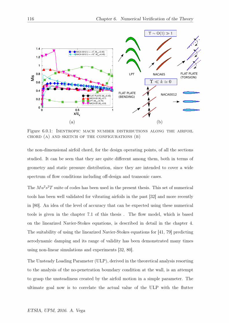
116 Chapter 6. Numerical Verification of the Theory
0 0.5 1
x/cx
0
0.2
0.4
0.6
0.8
1
1.2
1.4
Mis
FLAT PLATE (Min=0.45)
NACA 65 (Min=0.7)
LPT (Mexit
=0.75)
NACA 65 (Min=0.8)
0 0.5 1
x/cx
0
0.2
0.4
0.6
0.8
1
1.2
1.4
Mis
NACA 0012 (i = + 0o, M
exit=0.45)
NACA 0012 (i = +10o, M
exit=0.45)
LPT NACA65 FLAT PLATE
(TORSION)
FLAT PLATE
(BENDING)NACA0012
(a) (b)
Figure 6.0.1: Isentropic mach number distributions along the airfoilchord (a) and sketch of the configurations (b)
the non-dimensional airfoil chord, for the design operating points, of all the sections
studied. It can be seen that they are quite different among them, both in terms of
geometry and static pressure distribution, since they are intended to cover a wide
spectrum of flow conditions including off-design and transonic cases.
TheMu2s2T suite of codes has been used in the present thesis. This set of numerical
tools has been well validated for vibrating airfoils in the past [32] and more recently
in [80]. An idea of the level of accuracy that can be expected using these numerical
tools is given in the chapter 7.1 of this thesis . The flow model, which is based
on the linearized Navier-Stokes equations, is described in detail in the chapter 4.
The suitability of using the linearized Navier-Stokes equations for [41, 79] predicting
aerodynamic damping and its range of validity has been demonstrated many times
using non-linear simulations and experiments [32, 80].
The Unsteady Loading Parameter (ULP), derived in the theoretical analysis resorting
to the analysis of the no-penetration boundary condition at the wall, is an attempt
to grasp the unsteadiness created by the airfoil motion in a simple parameter. The
ultimate goal now is to correlate the actual value of the ULP with the flutter
ETSIA, UPM, 2016. A. Vega
117
characteristic of an airfoil, such as the phase of the influence coefficients, the minimum
and mean damping, etc.
The objective of this chapter is to quantitatively evaluate the Unsteady Loading
Parameter (ULP), to elucidate if the ULP is able to quantitatively predict the
influence of different aerodynamic loadings, reduced frequency and mode-shapes on
the aerodynamic damping. It is important to highlight that computing the ULP
does not require to perform unsteady simulations and, therefore, the use of this
parameter in the conceptual design phase can provide a quick assessment of the
flutter characteristics of bladed-disks. More interestingly, the prediction capability of
this parameter confirms the rationale of a large body of knowledge related with the
aerodynamics of os- cillating airfoils and its impact on the aerodynamic damping of
turbomachinery airfoils.
The correlation of the ULP with the work-per-cycle curves is not only a clear
indication of the understanding of the problem, but a conceptual tool to predict
the aerodynamic damping variations associated to design changes. In this section,
the problem of correlating the ULP with changes in:
1. Incidence and Mach number
2. Mode-shape
3. Airfoil geometry
is addressed, All the trends derived from the asymptotic analysis have been proved,
and the ULP is quantitatively correlated with the flutter characteristics of oscillating
airfoils. Both, the Influence Coefficient (IC) and the TravelingWave (TW) approaches
have been used in combination. The cascade constructed to run the simulations
using the IC formulation is made up of five airfoils in all the cases. The influence
of the number of airfoils of a linear cascade on the unsteady aerodynamics of
oscillating airfoils was investigated in [82] Nevertheless parallel studies were conducted
to investigate that five airfoil were enough to avoid the presence of artificial
perturbations transmitted through the periodic boundaries.
ETSIA, UPM, 2016. A. Vega

118 Chapter 6. Numerical Verification of the Theory
It has been concluded that all the aforementioned theoretical conclusions are
consistent with the numerical results presented here.
6.1 Relevance of the Rotational Contribution
For lightly steady loaded airfoils (∇W0 ' 0 ), the rotational contribution plays a
major role. For bending modes, the ULP is small (Υ ' 0), strictly zero for a flat plate
where ∇W0 = 0 . In this case the theory states, the IC moduli vary proportionally
with the reduced frequency, while the IC phases are constant, φ = π/2, which directly
implies that the work-per-cycle curves have a cosinusoidal shape. Nevertheless, for
steady lightly or unloaded airfoils vibrating in a torsion mode, (i.e.: α 6= 0), the
rotation contribution to the ULP is not zero, and then Υ 6= 0, which directly implies
that this type of cases should behave sanalogously to the loaded cases (i.e.: constant
lj with k, and small φ, which varies φ ∝ k, and sinusoidal shape of the work-per-cycle
curves). In order to verify this assertion, an asymmetric flat plate linear cascade,
vibrating in both flap and torsion has been studied, and the results for the work per-
cycle curves are presented together. The flow model, which is based on the linearized
Euler equations is described in the chapter 4.
6.1.1 Asymmetric Flat Plate Linear Cascade
The limiting case of a steady unloaded airfoil is a flat plate. For this reason, a linear
cascade of inviscid flat plates vibrating in torsion about the l.e. has been chosen as
the vehicle to verify that the ULP presented in this thesis can predict the behaviour
of vibrating airfoils at low reduced frequency, even when ∇W0c = 0. The flat plate
stagger angle is θ = 45ş, the Mexit = 0.45, and the pitch to chord ratio s/c = 0.5.
The cascade constructed to run the simulations using the IC formulation is made up
of five plates. This cascade has been used to investigate the bending mode as well.
When the steady loading is zero, and the surface normal does not change during
the blade vibration (pure bending modes), the ULP=0, and then, the phase of the
ETSIA, UPM, 2016. A. Vega
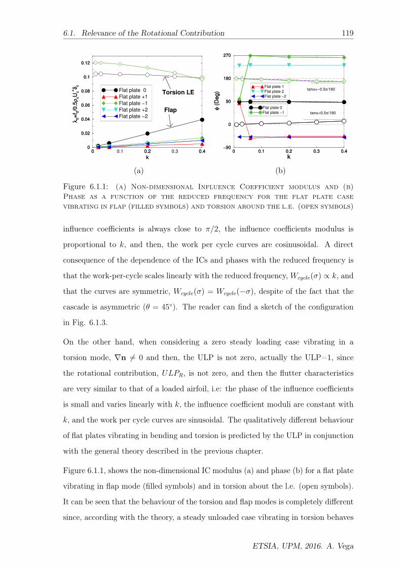
6.1. Relevance of the Rotational Contribution 119
0 0.1 0.2 0.3 0.4
k
0
0.02
0.04
0.06
0.08
0.1
0.12
λ0=
f 0/0
.5ρ
cU
c
2δ
c
Flat plate 0
Flat plate +1
Flat plate −1
Flat plate +2
Flat plate −2
0 0.2 0.4
k
0
0.02
0.04
0.06
0.08
0.1
0.12
λ0=
f 0/0
.5ρ
cU
c
2δ
c
Torsion LE
Flap
0 0.1 0.2 0.3 0.4
k
−90
0
90
180
270
φ (
De
g)
Flat plate 1
Flat plate 2
Flat plate −2
0 0.1 0.2 0.3 0.4
k
−90
0
90
180
270
φ (
De
g)
Flat plate 0
Flat plate −1 tanα=0.5π/180
tanα=−0.5π/180
(a) (b)
Figure 6.1.1: (a) Non-dimensional Influence Coefficient modulus and (b)Phase as a function of the reduced frequency for the flat plate casevibrating in flap (filled symbols) and torsion around the l.e. (open symbols)
influence coefficients is always close to π/2, the influence coefficients modulus is
proportional to k, and then, the work per cycle curves are cosinusoidal. A direct
consequence of the dependence of the ICs and phases with the reduced frequency is
that the work-per-cycle scales linearly with the reduced frequency,Wcycle(σ) ∝ k, and
that the curves are symmetric, Wcycle(σ) = Wcycle(−σ), despite of the fact that the
cascade is asymmetric (θ = 45). The reader can find a sketch of the configuration
in Fig. 6.1.3.
On the other hand, when considering a zero steady loading case vibrating in a
torsion mode, ∇n 6= 0 and then, the ULP is not zero, actually the ULP=1, since
the rotational contribution, ULPR, is not zero, and then the flutter characteristics
are very similar to that of a loaded airfoil, i.e: the phase of the influence coefficients
is small and varies linearly with k, the influence coefficient moduli are constant with
k, and the work per cycle curves are sinusoidal. The qualitatively different behaviour
of flat plates vibrating in bending and torsion is predicted by the ULP in conjunction
with the general theory described in the previous chapter.
Figure 6.1.1, shows the non-dimensional IC modulus (a) and phase (b) for a flat plate
vibrating in flap mode (filled symbols) and in torsion about the l.e. (open symbols).
It can be seen that the behaviour of the torsion and flap modes is completely different
since, according with the theory, a steady unloaded case vibrating in torsion behaves
ETSIA, UPM, 2016. A. Vega
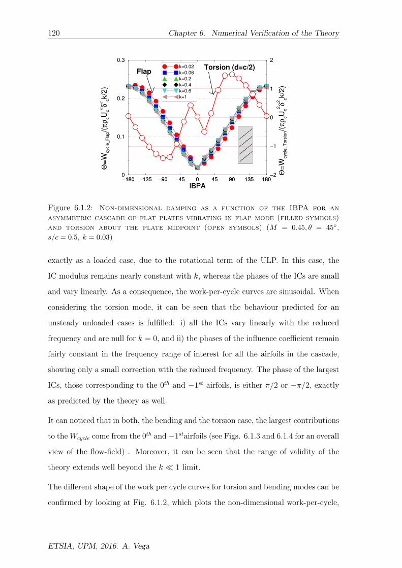
120 Chapter 6. Numerical Verification of the Theory
−180 −135 −90 −45 0 45 90 135 180
IBPA
0
0.1
0.2
0.3
Θ=
Wcycle
_F
lap/(
πρ
cU
c
2δ
2
ck/2
)
k=0.02
k=0.06
k=0.2
k=0.4
k=0.6
k=1
−180 −135 −90 −45 0 45 90 135 180
IBPA
−2
−1
0
1
2
Θ=
Wcycle
_T
ors
ion/(
πρ
cU
c
2δ
2
ck/2
)
Torsion (d=c/2)Flap
Figure 6.1.2: Non-dimensional damping as a function of the IBPA for anasymmetric cascade of flat plates vibrating in flap mode (filled symbols)and torsion about the plate midpoint (open symbols) (M = 0.45, θ = 45,s/c = 0.5, k = 0.03)
exactly as a loaded case, due to the rotational term of the ULP. In this case, the
IC modulus remains nearly constant with k, whereas the phases of the ICs are small
and vary linearly. As a consequence, the work-per-cycle curves are sinusoidal. When
considering the torsion mode, it can be seen that the behaviour predicted for an
unsteady unloaded cases is fulfilled: i) all the ICs vary linearly with the reduced
frequency and are null for k = 0, and ii) the phases of the influence coefficient remain
fairly constant in the frequency range of interest for all the airfoils in the cascade,
showing only a small correction with the reduced frequency. The phase of the largest
ICs, those corresponding to the 0th and −1st airfoils, is either π/2 or −π/2, exactly
as predicted by the theory as well.
It can noticed that in both, the bending and the torsion case, the largest contributions
to theWcycle come from the 0th and −1stairfoils (see Figs. 6.1.3 and 6.1.4 for an overall
view of the flow-field) . Moreover, it can be seen that the range of validity of the
theory extends well beyond the k 1 limit.
The different shape of the work per cycle curves for torsion and bending modes can be
confirmed by looking at Fig. 6.1.2, which plots the non-dimensional work-per-cycle,
ETSIA, UPM, 2016. A. Vega

6.1. Relevance of the Rotational Contribution 121
Θ1, defined as
Θ1 =Wcycle
12πρcv2
cδ2c k
. (6.1.1)
as a function of the IBPA, computed using the travelling-wave approach, for the same
plate, vibrating in bending (filled symbols), and in torsion about the midpoint of the
plate (open symbols), for different values of reduced frequency in the flap case and
for a reduced frequency of k = 0.03 for the torsion case. It can be seen that while
for the torsion mode the curves are of sinusoidal shape, for the bending mode, the
work-per-cycle curves are cosinusoidal in a wide range of reduced frequencies.
It may also be observed that for the bending case (ULP = 0), the damping curves
corresponding to a wide range of reduced frequencies nicely collapse into a single
universal curve, as predicted by the theoretical analysis, showing surprisingly that it
is not possible to destabilise the cascade decreasing the reduced frequency. It may
be seen that the theoretical predictions are valid well beyond the k 1, since even
the k = 1 case exhibits a good fit with the rest curves. The contribution in this
case of cascade airfoils different from the +0 and -1 is not small (see Fig. 6.1.1 (a)) ,
however in this case it may be observed that the phases of the ±2 airfoils are roughly
φ±2 = π/2±3π/4, and hence do not contribute to spoil the symmetry of the damping
curve.
It can be concluded that the different behaviour of a flat plate oscillating in bending
and torsion is strongly correlated with ULP and the theory derived for low-reduced
frequency, and is due to the contribution of the rotational part to the ULP.
The iso-contours of the real and imaginary, or in-phase and out-of-phase, parts of
the unsteady pressure of a flat plate vibrating in a torsion about the l.e. at k = 0.1
are displayed in Fig. 6.1.3. It can be noticed that, the real component is much
higher than the imaginary one, which is consistent with the fact that the unsteady
pressure phase is small. On the contrary, when considering the bending mode (see
Fig. 6.1.4 for more details), it can be seen that now the real component is much
smaller than the imaginary one, which is consistent with the fact that the phase is
±π/2. This different behaviour of the real an imaginary part between a bending
ETSIA, UPM, 2016. A. Vega

122 Chapter 6. Numerical Verification of the Theory
+1
0
-1
+1
0
-1
(a) (b)
Figure 6.1.3: Real (a) and imaginary (b) components of the unsteady pressurefor an asymmetric cascade of flat plates vibrating in torsion about the l.e.(Min = 0.45, θ = 45, s/c = 0.5, k = 0.1)
+1
0
-1
(a) (b)
Figure 6.1.4: (a) Real and (b) imaginary components of the unsteadypressure for an asymmetric cascade of flat plates vibrating in bending(Min = 0.45, θ = 45, s/c = 0.5, k = 0.1)
ETSIA, UPM, 2016. A. Vega

6.2. Steady Loading Effects 123
and a torsion case, even when considering the same cascade, with the same steady
loading„ is exactly as predicted by the theory.
6.2 Steady Loading Effects
In order to investigate the effect of the aerodynamic loading in the aerodynamic
damping, i.e.: changes in ∇W0 , different operating points have been studied for
an LPT airfoil and for the NACA 65 configuration. The NACA65 configuration will
also be used to explain the trends at reduced frequencies k ∼ O(1). It will be seen
that, although the way to obtain conclusions at high values of reduced frequency is
not rigorous, since the theoretical analysis has been done under the assumption that
k 1, it will be seen that the theory is able to explain many behaviours of the
work-per-cycle curves at values of reduced frequency k ∼ O(1), which is a surprising
fact. The vibration mode has been defined for all the cases as a rigid body flap mode
in a direction orthogonal to the engine axis. The trends derived from the ULP are
compared against that obtained solving the linearised Euler equations numerically.
6.2.1 LPT case off-design effect
An LPT airfoil has been considered in first place to check the ability of the ULP to
predict the aerodynamic damping of vibrating blades at low reduced frequency. The
design operating point is defined by an inlet and exit angle of α1 = 44 and α2 = 60,
respectively, Mexit = 0.75, and an airfoil spacing of s/c = 0.96. The aerodynamic
loading is changed by modifying the incidence with respect the aerodynamic design
point (ADP). Different operating points (OPs) have been studied, the ADP, a positive
off-design of 10 deg (name ADP+10), and a negative off-design of −24 deg (named
ADP-24). Linearised inviscid simulations were carried out using a grid containing
about 32,000 nodes per passage.
The results obtained for the ULP for the three OPs are shown in Table 6.1, while
Fig. 6.2.1 shows the isentropic Mach number distribution along the airfoil chord for
ETSIA, UPM, 2016. A. Vega

124 Chapter 6. Numerical Verification of the Theory
Incidence i = 0ş i = 10ş i = −24şULP 1.3 1.75 1.07
Table 6.1: Unsteady loading parameter value for the LPT configura-tion for different incidence angles
0 0.5 1
x/cx
0
0.5
1
1.5
2M
is
i=+0o
i=−24o
i=+10o
Figure 6.2.1: Isentropic Mach number distributions along the airfoil chordfor the LPT case for the design and off design conditions
the three cases. It can be ob- served that the velocity distributions only differ in
the front part of the airfoil, whereas the loading in the aft part of the blade remains
unchanged, as it was expected. It is important to remark that, in this case, the
spurious contribution to the ULP due to the acceleration around the rounded t.e.
of an inviscid flow (that is estimated in 0.7 for all the operating points) has been
manually removed. First of all, it can be noticed that the results obtained for the
ULP are consistent with the isentropic Mach number distributions: the highest value
of the ULP is the corresponding to the positive off design, whereas the lowest one is the
corresponding to the negative off design. The difference between the design case and
the negative off design case is smaller than the difference between the design case and
the positive off design case. According to the theory, the influence coefficient modulus
is proportional to the unsteady loading parameter, whereas the phase is proportional
to its inverse, which directly implies that the higher the ULP is, the more unstable
the configuration is, from a work-per-cycle point of view.
ETSIA, UPM, 2016. A. Vega

6.2. Steady Loading Effects 125
0 0.1 0.2 0.3
k
0.4
0.6
0.8
1
1.2
1.4
λ0=
f 0/0
.5ρ
cU
c
2δ
c
i=+0o
i=−24o
i=+10o
0 0.1 0.2 0.3
k
180
190
200
210
220
φ0 (
Deg)
i=+0o
i=−24o
i=+10o
tanα=2.5π/180
tanα=2π/180
tanα=1.5π/180
(a) (b)
Figure 6.2.2: (a) Non-dimensional Influence Coefficient modulus and (b)Phase of the central airfoil as a function of the reduced frequency forthe LPT case vibrating in flap mode for the different operating conditions
Figure 6.2.2 (a) represents the influence coefficients moduli for the vibrating airfoil
of the cascade, for the three operating points, whereas the phases of the influence
coefficient are shown in Fig.6.2.2 (b). It can be seen that the slope of the φ−k curves
and the IC moduli correlate very well with the unsteady loading parameter, since the
highest influence coefficient modulus and the lowest phase correspond to the highest
unsteady loading parameter (ADP+10), and the lowest influence coefficient modulus
and the highest phase are associated to the lowest unsteady loading parameter (ADP-
24). More precisely, the ratio of influence coefficient phases (or the ratio of the
influence coefficient modulus)at design and off-design conditions, e.g.: φ0,i=+0şφ0,i=+10ş
' 1.3,
is approximately the same as the ratio of the ULPs, i.e ULP0,i=+0şULP0,i=+10ş
' 1.3. Note that
in 6.2.2 (b) the slope of the φ − k curves at the origin are represented by means of
dashed lines, as well as its numerical values, to ease the understanding of the trends
in the low reduced frequency limit. The results for the ±1 airfoils of the cascade have
not been shown in this case in order to not overcrowd the plot, but the ULP is also
able to predict their behaviour in a qualitative manner, and it will be checked later
on for other cases.
Figure 6.2.3 shows the non dimensional work per cycle, Θ2, defined as:
Θ2 =Wcycle
12πρcv2
cδ2c
(6.2.1)
ETSIA, UPM, 2016. A. Vega

126 Chapter 6. Numerical Verification of the Theory
−180 −135 −90 −45 0 45 90 135 180
IBPA
−2
−1
0
1
2
Θ=
Wcycle/(
πρ
cU
c
2δ
c
2/2
)
i=+0o
i=−24o
i=+10o
Figure 6.2.3: Non-dimensional damping as a function of the IBPA and thesteady flow conditions for the low pressure turbine case vibrating in flap(M = 0.74, k = 0.1)
as a function of the IBPA, for the three operating points. In the same line as for the IC
approach, the damping curves follow the ULP trends, which can predict the stability
trend of the Wcycle curves. The ADP+10 operating point has the largest ULP, and
therefore is the most unstable configuration, whereas the ADP-24 operating point,
which has the smallest UDP, is the most stable.
The sensitivity of the Wcycle to the ULP=Υ is much smaller than that of the IC
modulus or phase. It is important to recall at this point (see [101] that:
φ ∼ k(1 + α∗Υ)
Υ(6.2.2)
whreas the non-dimensional IC moduli scales as lj ∼ Υ, hence the mean value of the
non-dimensional Wcycle is: Θmean ∼ k(1 + αΥ), and therefore its sensitivity to the
ULP is smaller than that of φ or lj, as it can be noticed in Fig. 6.2.3. The damping
variation with the IBPA, however, scales as ∆Θ ∼ Υ, and Fig. 6.2.3 is consistent
as well with this scaling. In general, the low sensitivity of the aerodamping of LPTs
with the incidence is in accordance with the existent experience.
ETSIA, UPM, 2016. A. Vega

6.2. Steady Loading Effects 127
6.2.2 NACA 65 Compressor
6.2.2.1 Off-design effects
The NACA65 compressor airfoil, [9, 99], has been chosen as the vehicle to prove that
the ULP can predict the behaviour of different types of geometries and also of airfoils
operating at transonic conditions, as long as they are in the low reduced frequency
range. Although compressors typically operate at higher reduced frequencies, it is
still interesting to understand the behaviour in the limit case of k 1 . Linearised
inviscid simulations were carried out using a grid containing about 16,000 nodes
per passage. The subsonic operating point (see [9, 99]) is defined by an inlet angle
α1 = 55ş , exit angle α2 = 40ş, inlet and exit isentropic Mach number, Min = 0.7
and Mexit = 0.45, respectively, and airfoil spacing, s/c = 1. In this operating point
the airfoil was operating at a positive off-design and then, the authors have decided
to study the design case by reducing the inlet angle by 3 deg (i = −3ş) with respect
to the standard case.
Figure 6.2.4 summarizes the isentropic Mach number distributions along the airfoil
chord for all the NACA65 cases, including the two subsonic operating conditions. It
can be seen that a variation of 3 deg in the incidence gives rise to a noticeable loading
modification in the front part of the airfoil. Table 6.2 shows the unsteady loading
parameter for the different off-design conditions. Figures 6.2.5 (a) and 6.2.5 (b)
display the non-dimensional influence coefficient moduli and phase for the NACA65
airfoil. It can be seen that, for the central airfoil, the influence coefficient modulus
of the design case is about twice that of the standard off-design case (l0,i=−3deg '
2∗l0,i=0deg) and that the slope of the φ−k curves is φ0,i=0deg ' 2∗φ0,i=−3deg, exactly as
predicted by the ULP, since Υi=−3deg ' 2∗Υi=0deg. It can be concluded that the ULP
is strongly correlated with the slope of the phase of the IC, and its modulus, when
the isentropic Mach number distribution is changed due to a change of the incidence.
The same behavior was obtained for the LPT airfoil, which has a completely different
shape and loading distribution. It is concluded that this observation is quite general
and that the ULP can quantitatively predicts off-design effects in the low re- duced
ETSIA, UPM, 2016. A. Vega

128 Chapter 6. Numerical Verification of the Theory
Incidence i = 0ş i = −3şULP 0.3 0.7
Table 6.2: Unsteady loading parameter for the NACA65 configuration fordifferent incidence angles at M1=0.7
0 0.5 1
x/cx
0
0.5
1
1.5M
is
i=+0o (M
1=0.7)
i=−3o (M
1=0.7)
i=+0o (M
1=0.8)
Figure 6.2.4: Isentropic Mach number distributions along the airfoil chordfor the NACA65 compressor for subsonic design and off design conditions,and for design transonic conditions
frequency limit.
6.2.2.2 Behaviour at k ∼ O(1)
Figure 6.2.6 (a) represents the modulus of the ICs as a function of the reduced
frequency. It may be observed that reduced frequency range of the plot extends
well beyond the low reduced frequency regime. When k ≤ 0.1 − 0.2 the ICs are
fairly constant, (see the inset of Fig. 6.2.6 (a)) however when k ∼o(1) the ICs
grow proportionally with k, exactly as it predicts the theory derived for k 1. It
is important to recall that the unsteady pressure associated solely to the vibration
velocity of the airfoil, not to the loading, is proportional to k. It can be seen as well
that only the 0th and −1st airfoils contribute significantly to theWcycle at low reduced
frequency.
ETSIA, UPM, 2016. A. Vega
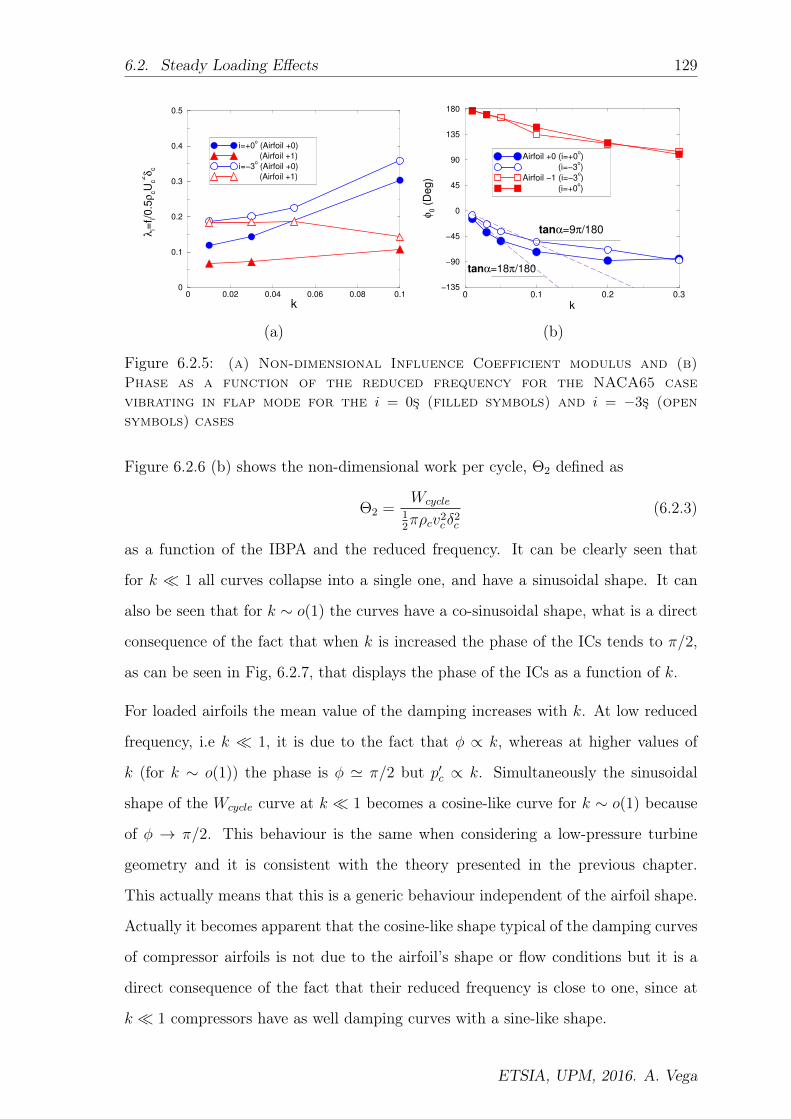
6.2. Steady Loading Effects 129
0 0.02 0.04 0.06 0.08 0.1
k
0
0.1
0.2
0.3
0.4
0.5
λi=
f i/0.5
ρcU
c
2δ
ci=+0
o (Airfoil +0)
(Airfoil +1)
i=−3o (Airfoil +0)
(Airfoil +1)
0 0.1 0.2 0.3
k
−135
−90
−45
0
45
90
135
180
φ0 (
De
g)
Airfoil +0 (i=+0o)
(i=−3o)
Airfoil −1 (i=−3o)
(i=+0o)
tanα=9π/180
tanα=18π/180
(a) (b)
Figure 6.2.5: (a) Non-dimensional Influence Coefficient modulus and (b)Phase as a function of the reduced frequency for the NACA65 casevibrating in flap mode for the i = 0ş (filled symbols) and i = −3ş (opensymbols) cases
Figure 6.2.6 (b) shows the non-dimensional work per cycle, Θ2 defined as
Θ2 =Wcycle
12πρcv2
cδ2c
(6.2.3)
as a function of the IBPA and the reduced frequency. It can be clearly seen that
for k 1 all curves collapse into a single one, and have a sinusoidal shape. It can
also be seen that for k ∼ o(1) the curves have a co-sinusoidal shape, what is a direct
consequence of the fact that when k is increased the phase of the ICs tends to π/2,
as can be seen in Fig, 6.2.7, that displays the phase of the ICs as a function of k.
For loaded airfoils the mean value of the damping increases with k. At low reduced
frequency, i.e k 1, it is due to the fact that φ ∝ k, whereas at higher values of
k (for k ∼ o(1)) the phase is φ ' π/2 but p′c ∝ k. Simultaneously the sinusoidal
shape of the Wcycle curve at k 1 becomes a cosine-like curve for k ∼ o(1) because
of φ → π/2. This behaviour is the same when considering a low-pressure turbine
geometry and it is consistent with the theory presented in the previous chapter.
This actually means that this is a generic behaviour independent of the airfoil shape.
Actually it becomes apparent that the cosine-like shape typical of the damping curves
of compressor airfoils is not due to the airfoil’s shape or flow conditions but it is a
direct consequence of the fact that their reduced frequency is close to one, since at
k 1 compressors have as well damping curves with a sine-like shape.
ETSIA, UPM, 2016. A. Vega

130 Chapter 6. Numerical Verification of the Theory
0 0.1 0.2 0.3
k
0
0.1
0.2
0.3
Airfoil 0
Airfoil +1
Airfoil −1
0 1 2 3
k
0
0.5
1
1.5
λi=
f i/0.5
ρcU
c
2δ
c
−180 −135 −90 −45 0 45 90 135 180
IBPA
−1
0
1
2
3
4
Θ=
Wcycle/(
πρ
cU
c
2δ
2
c/2
)
k=0.01
k=0.03
k=0.1
k=0.3
k=0.5
k=0.8
k=1
k=2
k=3
Unstable
Stable
(a) (b)
Figure 6.2.6: (a) Non-dimensional IC modulus of the 0th and ±1st airfoils asa function of the reduced frequency and (b) non-dimensional damping as afunction of the IBPA and the reduced frequency for the naca65 compressor(Min = 0.7)
0 0.5 1 1.5 2 2.5 3
k
−90
−45
0
45
90
135
180
φ (
Deg)
tanα=2π/180
tanα=4π/180 Airfoil 0
tanα=2π/180
tanα=1π/180
Airfoil +1
Airfoil −1
Figure 6.2.7: Phases of the 0th and ±1 airfoils as a function of the reducedfrequency for the naca65 compressor (Min = 0.7)
ETSIA, UPM, 2016. A. Vega

6.2. Steady Loading Effects 131
M1 M1 = 0.7 M1 = 0.8
ULP 0.3 -0.17
Table 6.3: Unsteady loading parameter for the NACA65 configuration fordifferent inlet Mach number
6.2.3 NACA 65 Mach number effects
In order to check that the ULP can predict changes in the loading distribution
associated to variations in the Mach number, the inlet Mach number was raised
from Min = 0.7 to Min = 0.8, driving the airfoil into the transonic regime.
Figure 6.2.4 displays the isentropic Mach number distributions along the airfoil chord
for both inlet Mach numbers, whereas Table 6.3 shows the corresponding ULP for
these two cases.
The transonic case exhibits a strong shock wave in the suction side that is clearly
visible in the isentropic Mach number distribution. It is very interesting to notice
that the ULP for the transonic case is significantly lower than that of the subsonic
case. This fact is reflected in the influence coefficient moduli and phases (Fig. 6.2.8
(a) and (b)). It can be seen that, in the region where the theory is applicable (k 1),
the influence coefficient modulus of the vibrating airfoil is the double for the subsonic
case than for the transonic case, and that the influence coefficient moduli of the other
airfoils of the cascade is smaller for the transonic than for the subsonic conditions.
The influence coefficient phases follow the expected trends as well: the slope of the
φ− k curves is higher for the subsonic than for the transonic case.
For the transonic case, the low reduced frequency theory is only valid for very low
values of the reduced frequency because the ULP is very low. Remember that the
theory states that an airfoil behaves as a loaded airfoil if ∇Wc ∼ ULPk. If the
unsteady loading is small, the range of k at which the airfoil behaves as a loaded airfoil
(constant IC with k, and small pressure phase) is very narrow. In our case, the IC
modulus does not remain constant with the reduced frequency and the phase of the
airfoil 0 is −π/2. The negative sign of the ULP predicts that, on the contrary than for
the subsonic case, the highest contribution to the work-per-cycle comes from the +1
ETSIA, UPM, 2016. A. Vega

132 Chapter 6. Numerical Verification of the Theory
0 0.025 0.05 0.075 0.1
k
0
0.1
0.2
0.3
0.4
0.5
0.6
0.7
0.8λ
i=f i/0
,5ρ
cU
c
2δ
cM
1=0.8 (Airfoil +0)
(Airfoil +1)
(Airfoil −1)
M1=0.7 (Airfoil +0)
(Airfoil +1)
(Airfoil −1)
0 0.1 0.2 0.3 0.4 0.5
k
−90
−45
0
45
90
135
180
225
270
φ (
deg)
tanα=−18π/180
tanα=8π/180tanα=−2π/180
tanα=−8π/180
tanα=3π/180
(a) (b)
Figure 6.2.8: (a) Non-dimensional Influence Coefficient modulus and (b)Phase as a function of the reduced frequency for the NACA65 casevibrating in flap mode. M1 = 0.8: filled symbols and M1 = 0.7: open symbols.
airfoil (the blade numbering sign criterion is defined in Fig. 6.2.9). Figure 6.2.9 (a)
displays the real and imaginary part of the unsteady pressure for the transonic case.
It can be seen that the presence of the shock wave generates a high level of unsteady
pressure in its vicinity, and then, the unsteady pressure distribution completely differs
from that observed for the subsonic case (see Fig. 6.2.9 (b))
6.3 Mode shape effects
The capability of the ULP to predict the effect of the bending direction on the
modulus and phase of the ICs has been studied for the LPT case operating at design
conditions and for the NACA 65 compressor operating at subsonic conditions. The
motion of a blade as a rigid body about an arbitrary torsion centre can be seen as
a linear combination of a flap, an edge-wise, and a torsion mode. The predictions of
the analytical trends for the flap and edge modes, are compared against numerical
results for the LPT, and the NACA65 configurations. For the LPT, the torsion
mode is also studied. The motion of an airfoil as a rigid body about an arbitrary
torsion centrecenter can be seen as a linear combination of a flap, an edge-wise, and
a torsion mode [90]. The predictions based on the ULP are compared against the
actual numerical results for the LPT and the NACA65 configurations oscillating in
ETSIA, UPM, 2016. A. Vega

6.3. Mode shape effects 133
0
+1
-1
(a)
0
+1
-1
(b)
Figure 6.2.9: Real (Left) and Imaginary (Right) part of the unsteady pressureof the NACA65 Compressor for k = 0.1, for Min = 0.8 (a) and for Min = 0.7 (b)
ETSIA, UPM, 2016. A. Vega

134 Chapter 6. Numerical Verification of the Theory
ULP Effect F E LE c/4 c/2 3c/4
Loading 1.93 0.92 1.39 0.3 0.11 -0.5Rotation 0 0 1.15 1.15 1.15 -1.15
Table 6.4: Unsteady loading parameter for the LPT configuration for thetwo fundamental bending directions and different torsion centres
the bending and edge-wise modes.
6.3.1 LPT Design Case
The ULP has been evaluated for the edge-wise, flap, and several torsion modes.
According to the results, summarised in Table 6.4 (note that the values for the ULP
summarised in this table include the t.e. contribution, that was removed in the
subsection “Steady Loading Effects”). In accor- dance with the ULP values computed
for the flap and edge-wise modes (First two columns in Table 6.4) we should obtain
that l0,FLAP ' 2 · l0,EDGE and φ0,EDGE ' 2 · φ0,FLAP ; and, as a consequence, the
airfoil is more unstable vibrating in the bending than in edge-wise direction.
This statement can be confirmed by looking at the non dimensional work-per-cycle
curves, represented in Fig. 6.3.1, for the reduced frequency k = 0.1. It can be seen
that the mean values are almost the same for the two modes whereas the amplitude
of the sinuosoidal variation of the aerodynamic damping with the IBPA for the flap
mode is about twice as big as that corresponding to the edge mode, as predicted
by the theory. The different trend of the IC modulus and phase (see Fig. 6.3.2 (a)
and (b) respectively) of the flap and edgewise modes with the reduced rfequency
correlates very well quantified with the ULP for the central airfoil, and it is also well
predicted for its neighbouring airfoil.
Torsion modes have also been investigated. Different torsion centres, all of them with
a fixed vibration amplitude of 1 deg, have been considered, namely: a torsion about
the l.e. and rotations about centres placed at a distance of c/2, c/4 and 3c/4 from the
l.e., where here c represents the true chord. The ULP values are presented together
with the corresponding to the bending modes, in Table 6.4. The total unsteady
loading parameter for the torsion mode is the sum of the two contributions (the
ETSIA, UPM, 2016. A. Vega

6.3. Mode shape effects 135
−180 −135 −90 −45 0 45 90 135 180
IBPA
−2
−1.5
−1
−0.5
0
0.5
1
1.5
2
Θ=
Wcycle/(
πρ
cU
c
2δ
c
2/2
)
TC c/4 (ULP=+1.55)
c/2 (ULP=+1.35)
3c/4 (ULP=−1.65)
LE (ULP=+2.55)
−180 −135 −90 −45 0 45 90 135 180
IBPA
−2
−1.5
−1
−0.5
0
0.5
1
1.5
2
Θ=
Wcycle/(
πρ
cU
c
2δ
c
2/2
)
Edge (ULP= 0.92)
Flap (ULP= 1.93)
Figure 6.3.1: Non-dimensional work as a function of the IBPA for the LPTcase vibrating in flap, edge and different torsion modes (M = 0.74, k = 0.1)
0 0.1 0.2 0.3
k
0.2
0.4
0.6
0.8
1
λi=
f i/0.5
ρcU
c
2δ
c
Airfoil +0 (Flap)
(Edge)
Airfoil +1 (Edge)
(Flap)
0 0.1 0.2 0.3
k
135
180
225
φ0 (
Deg)
Airfoil +0 (Flap)
(Edge)
Airfoil +1 (Edge)
(Flap)tanα=3π/180
tanα=2π/180
+180
+180
(a) (b)
Figure 6.3.2: (a) Non-dimensional IC modulus and (b) phase as a function ofthe reduced frequency for the LPT case vibrating in flap (filled symbols)and edge mode (open symbols).
ETSIA, UPM, 2016. A. Vega

136 Chapter 6. Numerical Verification of the Theory
steady loading contribution and the rotational contribution), and then the total ULP
parameters are ΥTORSIONLE ' 2.46, ΥTORSIONc/4 ' 1.47, ΥTORSIONc/2 ' 1.3 and
ΥTORSION3c/4' −1.65.
When looking at the non dimensional work per cycle curves (Fig. 6.3.1) it can be seen
that the instability level is perfectly aligned with the simplified results predicted using
the ULP. For the torsion about the centre placed at a distance of 3c/4 from the l.e.,
the ULP is negative; as it has been previously mentioned, this is an indication that
the neighbouring airfoil with the largest contribution to the work per cycle is located
at the opposite side of the central airfoil, in this case -1 profile. This fact directly
implies that the minimum damping occurs at IBPA=-90ş instead of at IBPA=90ş.
This behaviour can be confirmed by looking at the damping curves, Fig. 6.3.1. The
effect of the sign of the ULP onto the neighbour airfoils and, as a consequence, onto
the Wcycle curves was reported for the NACA65 configuration when comparing the
subsonic and the transonic conditions, in the subsection “Steady Loading Effects”.
6.3.2 NACA65 Subsonic Case
Analogously to the LPT case, the ULP is now evaluated for the NACA 65 operating
at subsonic conditions for different mode-shapes. Analytical results for the ULP are
presented in Table 6.5. The analytical solution shows that ΥEDGE ' 5.5 · ΥFLAP .
According to this, it should be obtained from the linearised Euler solver that
l0,EDGE ' 5.5 · l0,FLAP and φ0,FLAP ' 5.5 ·φ0,EDGE; and then, contrary to the general
behaviour of the LPT airfoils, the edge mode should be more unstable than the flap
mode. It is very important to note that the negative sign of the ULP denotes that
the highest contribution to the work per cycle comes from the opposite neighbouring
airfoil i.e: for the flap mode the -1 airfoil is the one contributing the most, while
for the edge mode the +1 airfoil has the highest contribution. This trend can be
confirmed by analyzing Fig. 6.3.3, which represent the non-dimensional IC moduli
and phase, obtained from the numerical simulations. It can be seen that, from the
IC point of view, there is a very good correlation between the influence coefficient
ETSIA, UPM, 2016. A. Vega

6.4. Geometry Effects 137
Mode shape Flap EdgeULP 0.294 -1.63
Table 6.5: Unsteady loading parameter for the NACA65 configuration forthe two fundamental bending directions
0 0.05 0.1 0.15 0.2
k
0
0.5
1
1.5
λi=
f i/0.5
ρcU
c
2δ
c
Flap (Airfoil +1)
(Airfoil −1)
Edge (Airfoil +1)
(Airfoil −1)
0 0.05 0.1 0.15 0.2
k
0
0.5
1
1.5
λi=
f i/0.5
ρcU
c
2δ
c
Airfoil +0 (Flap)
(Edge)
0 0.1 0.2 0.3 0.4 0.5
k
−90
−45
0
45
90
135
180
225
270
φ (
deg)
Airfoil 0
−1
+1
tanα=17π/180
tanα=8π/180
tanα=−2π/180
tanα=−8π/180
tanα=3π/180
(a) (b)
Figure 6.3.3: (a) Non-dimensional IC modulus and (b) phase as a functionof the reduced frequency for the NACA65 case vibrating in flap (filledsymbols) and edge mode (open symbols)
modulus and phase, even for the neighbouring airfoils, with the ULP, that actually
predicts very well their trends.
It can be seen that the theory is valid for a larger range of k for the edge mode than
for the flap: i.e the range of k at which φ0 varies linearly and l0 remains constant;
this is a direct consequence that the ULP of the flap mode is much smaller than that
of the edge mode.
6.4 Geometry Effects
In the previous subsections, the effect of the aerodynamic loading and the vibration
mode onto the unsteady aerodynamics of oscillatingting airfoils at low reduced
frequency has been investigated. It has been proved that the ULP can predict with
an acceptable degree of accuracy, the variations onto the ICs modulus and phase,
and the work-per-cycle curves when a modification, either in the design operating
conditions or in the vibration mode shape, is introduced. It is necessary the reader
ETSIA, UPM, 2016. A. Vega
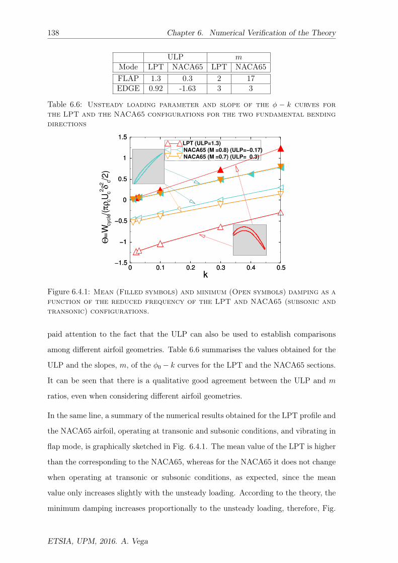
138 Chapter 6. Numerical Verification of the Theory
ULP mMode LPT NACA65 LPT NACA65FLAP 1.3 0.3 2 17EDGE 0.92 -1.63 3 3
Table 6.6: Unsteady loading parameter and slope of the φ − k curves forthe LPT and the NACA65 configurations for the two fundamental bendingdirections
0 0.1 0.2 0.3 0.4 0.5
k
−1.5
−1
−0.5
0
0.5
1
1.5
Θ=
Wcycle/(
πρ
cUc2
δ2
c/2
)
LPT (ULP=1.3)
NACA65 (M =0.8) (ULP=−0.17)
NACA65 (M =0.7) (ULP= 0.3)
0 0.1 0.2 0.3 0.4 0.5
k
−1.5
−1
−0.5
0
0.5
1
1.5
Figure 6.4.1: Mean (Filled symbols) and minimum (Open symbols) damping as afunction of the reduced frequency of the LPT and NACA65 (subsonic andtransonic) configurations.
paid attention to the fact that the ULP can also be used to establish comparisons
among different airfoil geometries. Table 6.6 summarises the values obtained for the
ULP and the slopes, m, of the φ0 − k curves for the LPT and the NACA65 sections.
It can be seen that there is a qualitative good agreement between the ULP and m
ratios, even when considering different airfoil geometries.
In the same line, a summary of the numerical results obtained for the LPT profile and
the NACA65 airfoil, operating at transonic and subsonic conditions, and vibrating in
flap mode, is graphically sketched in Fig. 6.4.1. The mean value of the LPT is higher
than the corresponding to the NACA65, whereas for the NACA65 it does not change
when operating at transonic or subsonic conditions, as expected, since the mean
value only increases slightly with the unsteady loading. According to the theory, the
minimum damping increases proportionally to the unsteady loading, therefore, Fig.
ETSIA, UPM, 2016. A. Vega

6.5. Mach Number Effect 139
6.4.1 shows that the most unstable configuration is the LPT airfoil, because it is the
one with the largest ULP, and that the NACA 65 airfoil is more unstable operating at
Min = 0.7 than atMin = 0.8, because of the ULP parameter is higher for the subsonic
conditions than for the transonic conditions. It can be seen that in the same scale, the
variation of the minimum damping for the NACA65 when moving from the subsonic
to the transonic conditions is small, when it is compared with the corresponding
value for the LPT. This fact is consistent with the values calculated for the ULP,
since ΥLPT ' 6 ·ΥNACA65,transonic and ΥNACA65,subsonic ' 1.6 ·ΥNACA65,transonic.
It can be concluded that the ULP can qualitatively compare different airfoils, but
is much better when comparing the same airfoil at different operating points and
mode-shapes.
6.5 Mach Number Effect
6.5.1 Phasing Variation
The effect of the Mach number in the conclusions derived in this thesis is investigated
by means of the LPT configuration previously presented. The vibration mode shape
chosen is a flap mode, although all the conclusions presented here apply to other
mode-shapes. The results presented within this section correspond to viscous cases.
The phase of the unsteady pressure of the central and +1 airfoils with respect the
airfoil displacement, φ, plays a central role in the overall work of the system and
therefore it has been inspected in great detail. Figure 6.5.1 shows the dependence of
the influence coefficient phase of the central, φ0, and +1, φ+1, airfoils as a function
of the reduced frequency and Mach number. It may be seen that both, in a large
range of reduced frequencies, scale linearly, as predict by the theory. It can also be
seen that the sensitivity to the Mach number is fairly slow, so it can be concluded
that compressibility is a second order effect, which only takes place through a slight
modification of the airfoil loading shape, as it will be explained later on in the
“Physical Interpretation” section. The effect of the change in the dynamc head is
ETSIA, UPM, 2016. A. Vega

140 Chapter 6. Numerical Verification of the Theory
0 0.1 0.2 0.3 0.4
k
0
20
40
φ (
Deg)
M2=0.6
M2=0.75
M2=0.185
M2=0.53
tan α = 2π/180
tan α = 1π/180
Airfoil 0
Airfoil +1
Figure 6.5.1: Phase of the influence coefficients of the 0th and +1st airfoilsas a function of the Reduced frequency and Mach numbers for a LPTairfoil.
well captured and the secondary role of Mach number effects, neglected in the theory,
confirmed.
As it was already explained in the previous chapter, if it is assumed that the influence
of all the airfoils, except that of the central and adjacent airfoils, can be neglected in
the work per cycle (see [5] and Fig.6.5.2) then:
Wcycle = −πp′cδcc[l0 sinφ0 + l+1 sin(φ1 + σ) + l−1 sin(φ−1 − σ)
](6.5.1)
where lj and φj are respectively the non-dimensional modulus and phase of the jth
influence coefficient, and δc the modulus of the vibration amplitude. Moreover if the
reduced frequency is small enough, and therefore φj 1, and if l−1 l+1 (which
is frequently seen in aerodynamically loaded oscillating airfoils), then the expression
6.5.1, neglecting second order terms, reduces to:
Wcycle = −πδ2c l+1
[(l0
l+1
)φ0 + sin(φ1 + σ)
], (6.5.2)
Where, it can be seen that the phase of the 0th influence coefficient is responsible
of the work-per-cycle increase with k (the stabilisation of the work per cycle curves
with the reduced frequency), which in first approximation is linear since the phase
is linear with the reduced frequency; actually it is φ0 ' 2k for this case. The phase
of the +1 airfoil is responsible of the shift of the minimum work-per-cycle location.
ETSIA, UPM, 2016. A. Vega
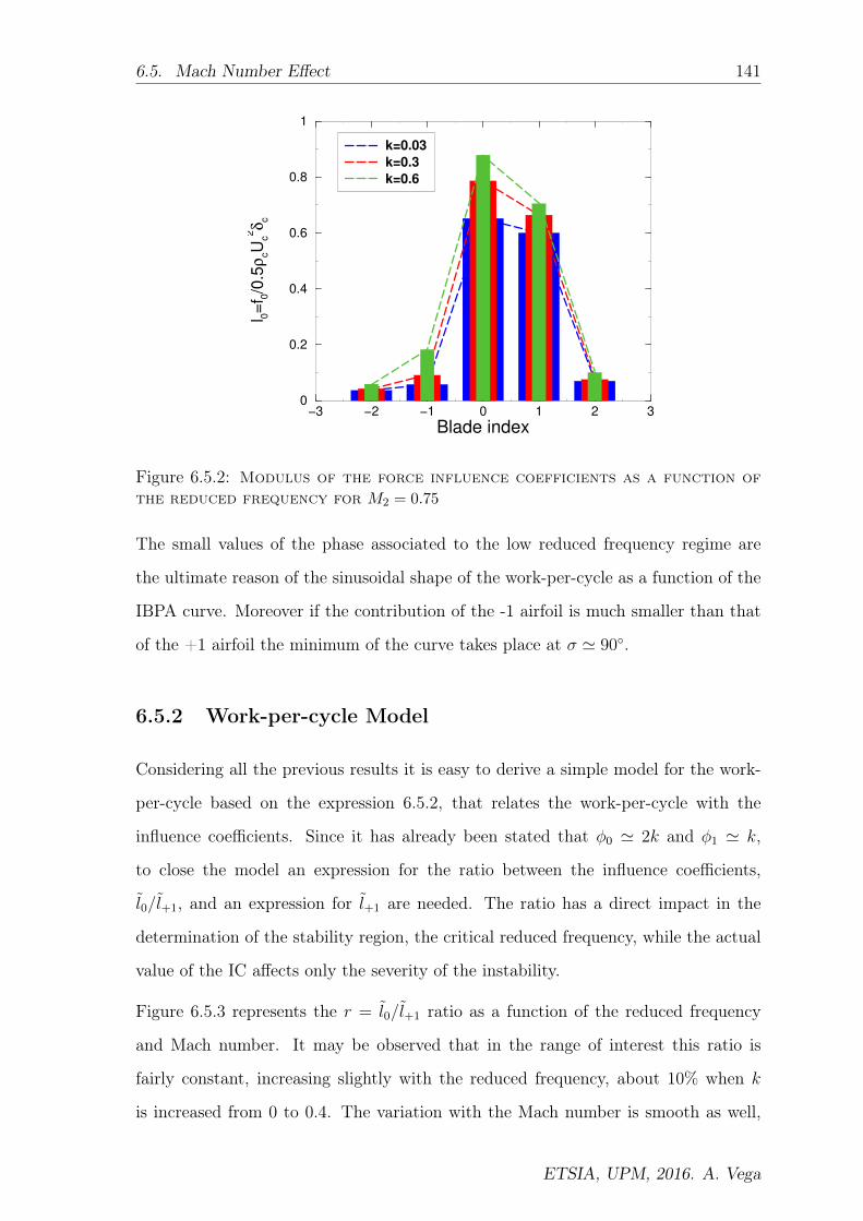
6.5. Mach Number Effect 141
−3 −2 −1 0 1 2 3
Blade index
0
0.2
0.4
0.6
0.8
1
l 0=
f 0/0
.5ρ
cU
c
2δ
c
k=0.03
k=0.3
k=0.6
Figure 6.5.2: Modulus of the force influence coefficients as a function ofthe reduced frequency for M2 = 0.75
The small values of the phase associated to the low reduced frequency regime are
the ultimate reason of the sinusoidal shape of the work-per-cycle as a function of the
IBPA curve. Moreover if the contribution of the -1 airfoil is much smaller than that
of the +1 airfoil the minimum of the curve takes place at σ ' 90.
6.5.2 Work-per-cycle Model
Considering all the previous results it is easy to derive a simple model for the work-
per-cycle based on the expression 6.5.2, that relates the work-per-cycle with the
influence coefficients. Since it has already been stated that φ0 ' 2k and φ1 ' k,
to close the model an expression for the ratio between the influence coefficients,
l0/l+1, and an expression for l+1 are needed. The ratio has a direct impact in the
determination of the stability region, the critical reduced frequency, while the actual
value of the IC affects only the severity of the instability.
Figure 6.5.3 represents the r = l0/l+1 ratio as a function of the reduced frequency
and Mach number. It may be observed that in the range of interest this ratio is
fairly constant, increasing slightly with the reduced frequency, about 10% when k
is increased from 0 to 0.4. The variation with the Mach number is smooth as well,
ETSIA, UPM, 2016. A. Vega

142 Chapter 6. Numerical Verification of the Theory
0 0.1 0.2 0.3 0.4
k
1
1.1
1.2
1.3
1.4
λ0/λ
1
M2=0.75
M2=0.6
M2=0.185
Figure 6.5.3: Ratio between the modulus of influence coefficient 0 and +1as a function of the Reduced frequency and Mach number
the ratio drops about 10% when Mexit is changed from 0.2 to 0.75. Hence, the ratio
between the ICs can be modelled as r = r0 + αk, with r0 ' 1.1 and α ' 0.2 for this
particular case.
For a flapping mode the exit angle of all the airfoils of the cascade is the same and
then, the total lift generated by them must be constant, in a quasi-steady regime. The
lift increase generated in the central airfoil when it moves downwards and the pitch of
the suction side passage is increased has to be balanced by the lift decrease of the +1
airfoil, that sees a decrease of the pitch of its suction side passage. Therefore, l0 ' l+1
in first approximation, irrespectively of the reduced frequency and the Mach number.
The missing lift (around 10% in this case) is compensated by the contribution of the
rest of the airfoils.
The critical reduced frequency, kc, may be derived from:
(r0 + αkc)2kc − 1 = 0. (6.5.3)
The most important conclusion is that the stability limit is weakly dependent on the
Mach number.
Figure 6.5.4 describes the variation of the non-dimensional influence coefficient
ETSIA, UPM, 2016. A. Vega

6.5. Mach Number Effect 143
0.1 0.2 0.3 0.4 0.5 0.6
M2
2
0.6
0.7
0.8
0.9
1
λ0=
f 0/0
.5ρ
cU
c
2δ
c
k=0.35
k=0.2
k=0.15
k=0.1
k=0.05
Figure 6.5.4: Variation of the influence coefficient of the central bladewith the square of the Mach number and the reduced frequency
modulus of the central airfoil with k and M . It may be seen that the variation
with the Mach number squared, or the dynamic head, is properly absorbed by
the non-dimensionalisation since the variation of the IC with M2exit in the range
Mexit ∈ [0.4− 0.7] is of second order compared with the variation of k, that is small
as well, of the order of 10% in the range k ∈ [0− 0.2].
The previous effect is a clear indication that the unsteady pressure scales
proportionally to the dynamic head, exactly as it was predicted by the theoretical
analysis. The effect of the Mach number is then in first approximation to increase
the severity of the instability due to the fact that l0 ∝ M2 , or more precisely,
l0 ∝ 12ρcU
2c f(M), but it does not significantly change the stability limit, since ratio of
the influence coefficient modulus, r = l0/l1 is fairly constant with the Mach number.
The dependence of the IC with the reduced frequency may be derived from the same
figure, and is of the form: l0 = (l0)k=0+(dl0/dk)k=0 k, where the linear correction with
k is small for loaded airfoil and low reduced frequencies, as it has been demonstrated
theoretically.
These two facts may be verified deriving directly the damping as a function of the
IBPA for different Mach numbers. Figure 6.5.5 represents the variation with the
ETSIA, UPM, 2016. A. Vega

144 Chapter 6. Numerical Verification of the Theory
Mach Number of the non-dimensional work, obtained using the TW formulation. It
may be observed that while the effect of changing only the reduced frequency but not
the Mach Number is a shift in the work-per-cycle curve and an increase in the mean
work, the effect of the Mach number is in first approximation very small, much less
obviously than that of the dimensional influence coefficient displayed in Fig. 6.5.4.
The weak effect of changing the M onto the Wcycle curves is due to the fact that the
effect of the Mach on the dynamic pressure has already been retained in the non-
dimensionalisation of the influence coefficient moduli, while the effect of the acoustics
(the effect of the M on the influence coefficient phase) has been shown to be small
and therefore all the curves tend to coalesce in a single one, especially in the minimum
damping region.
Since the variation of Wcycle with M is solely due to the variation of r = l0/l1 with
M , which is small as well, the curves for different values of M still exhibit a small
scaling effect, since changing the Mach number for a given geometry gives rise to a
significant change of the airfoil loading, that is superimposed to the Mach number
change (see Fig. 6.5.7). However, the stability region is fairly unaffected, as it was
claimed before. Figure 6.5.6 shows the amplitude of the mean and 1st harmonic (the
variation with the IBPA) of the non-dimensional work as a function of the square of
the Mach number. It can be still seen that both scale weakly with Mach Number
square.
Note that since k 1 and α ' 0.2⇒ αk r0 ⇒ r ' r0; therefore, a model for the
work per cycle for this mode can be written according to the following formula:
Wcycle = −πβq20 [2r0k + sin(k + σ)] (6.5.4)
where β = (P0 − pexit)c = P0cF(M2exit) and, if M2
exit(γ − 1)/2 1, then
β ' γ
2p0M
2exit '
1
2ρexitV
2exit (6.5.5)
(note that, for M = 0.7, M2exit(γ − 1)/2M2
exit ' 0.1 1). Note that the Wcycle is
proportional to the dynamic head at the exit, that scales as the square of the Mach
number, exactly as shown in Fig. 6.5.4, where the explicit dependence with M2exit
ETSIA, UPM, 2016. A. Vega

6.5. Mach Number Effect 145
−180 −90 0 90 180
IBPA
−1.5
−1
−0.5
0
0.5
1
1.5
2
2.5
ΘI=
Wcycle/(
πρ
c
2
δc
2U
c
2/2
)
M2=0.185 (k=0.3)
M2=0.6 (k=0.3)
M2=0.5 (k=0.3)
M2=0.75 (k=0.3)
M2=0.75 (k=0.03)
Figure 6.5.5: Non-dimensional work as a function of the IBPA and the Machnumber
0 0.2 0.4 0.6
M2
2
4
6
8
10
12
14
ΘI=
W/(
πρ
infU
inf2δ
2h/2
)
Mean Value
1st
harmonic
Figure 6.5.6: Mean value and variation with the IBPA of the non-dimensionalwork as a function of the mach number
ETSIA, UPM, 2016. A. Vega

146 Chapter 6. Numerical Verification of the Theory
0 0.5 1
x/cx
0
0.5
1
1.5
Mis/M
2 M2 =0.75
M2 =0.5
M2 =0.4
M2 =0.185
M2 =0.6
Figure 6.5.7: Isentropic Mach number distribution normalized with the exitMach number for different exit Mach numbers.
has been absorbed by the non-dimensionalisation. This is a comprehensive model for
Wcycle that retains the influence of both the Mach and the reduced frequency.
Figure 6.5.8 represents a sketch which summarises the effect of both, the reduced
frequency and the Mach number onto the stability and the trends of the work-per-
cycle curves. This figure can be explained as follows: departing from a cas in the
k 1 range, whose work-per-cycle curve is be similar to the blue line, if the reduced
frequency is increased and the Mach number is maintained constant, the effects on
the curve can be seen looking at marron curve, which are an increase in the mean
value and a shift in the IBPA where ocurrs the minimum, towards the IBPA = 0ş.
Departing from this situation, if the reduced frequency is frozen and the Mach number
is increased, it can be seen that the effect is an increase in the severity of the instability
(see pink curve).
ETSIA, UPM, 2016. A. Vega

6.6. Symmetric cascades 147
Figure 6.5.8: Effect of the reduced frequency and the M onto the work-per-cycle curves
6.6 Symmetric cascades
6.6.1 NACA 0012 Symmetric Case
A NACA 0012 section has been chosen to build a linear symmetric cascade and
verify the theoretical conclusions derived for symmetric loaded configurations. Both
the inlet and outlet flow angles are α1,2 = 0ş , the exit isentropic Mach number
is Mexit = 0.45, and the pitch to chord ratio s/c = 1. For the asymmetric case,
constructed with the same airfoil, the boundary conditions are the same, except for
the fact that an inlet angle of 10ş is considered. Linearised inviscid simulations have
been carried out using grids containing about 45,000 nodes per passage.
Symmetric cascades with symmetric airfoils are a particular case, which implies that
with a general character, l+1 = −l−1 and φ−1 = π + φ+1. As it has been already
outlined in the previous chapter, Wcycle(σ) ∝ k and the Wcycle curves are symmetric,
i.e Wcycle(σ) = Wcycle(−σ) . Figure 6.6.2 (b) shows the dependence of the influence
coefficient phase of the central, φ0, and ±1, airfoils, φ±1, as a function of k. It may
be seen that all of them, in a large range of reduced frequencies, scale linearly with
ETSIA, UPM, 2016. A. Vega

148 Chapter 6. Numerical Verification of the Theory
0
+1
-1
Figure 6.6.1: Snapshot of the unsteady pressure for the NACA0012 symmetriccase for k = 0.2
the reduced frequency and that φ−1 = π + φ+1, as expected for a symmetric case. In
the same line, Fig. 6.6.1,which represents a snapshot of the unsteady pressure for a
k = 0.2 case, shows that the unsteady behavior of this case is symmetric.
The moduli of the ICs , represented in Fig. 6.6.2 (a), follow two different trends
because the NACA 0012 is a lightly loaded section compared with the LPT or NACA
65 sections. Figure 6.0.1 shows how the Mach number or the velocity gradient along
the airfoils chord, which is actually only a part of the contribution to the gradient, is
very small for the NACA 0012, being this case an intermediate case between a highly
loaded case and a flat plate with strictly zero loading. This means that the range of
reduced frequencies at which the ICs remain constant is much narrower than in the
NACA 65 or LPT cases. As a consequence, the ICs exhibit a small constant region
for k < 0.1, in the same way than highly loaded profiles, and for k > 0.1 a linear
increase with k, exactly as in the flat plate (unloaded) case.
For a loaded symmetric profile the work-per cycle scales with the reduced frequency
ETSIA, UPM, 2016. A. Vega

6.6. Symmetric cascades 149
0 0.1 0.2 0.3 0.4 0.5
k
0
0.1
0.2
0.3
0.4
0.5
λ i=
f i/0.5
ρcU
c
2δ
c
Airfoil −1 (i=+100)
Airfoil 0 (i=+100)
Airfoil +1 (i=+100)
Airfoil 0 (i=+00)
Airfoil +1 (i=+00)
0 0.1 0.2 0.3 0.4 0.5
k
−60
0
60
120
180
φ (
Deg)
Airfoil 0 (i=+00)
Airfoil +1 (i=+00)
Airfoil 0 (i=+100)
Airfoil −1 (i=+100)
Airfoil −1 (i=+00)
tanα=3π/180
tanα=2π/180
tanα=2π/180
(a) (b)
Figure 6.6.2: (a) Non-dimensional IC modulus and (b) phase of the 0th and±1st airfoils as a function of the reduced frequency for the NACA 0012symmetric (filled symbols) and asymmetric (open symbols) cases.
as follows:
Θ1 =Wcycle
12πρcv2
cδ2c k
(6.6.1)
The non-dimensional Wcycle curves for different values of k are displayed in Fig. 6.6.3
(a), where it can be clearly seen that all curves nicely collapse into a single cosine-
like shape curve, in a wide range of reduced frequencies, which tightly follows the
theoretical predictions well beyond the low reduced frequency limit.
The region −45 < σ < 45 exhibit a series of peaks whose amplitude is determined
by its separation to the resonant conditions. Since resonances change with k, while
the matrix of computed IBPAs is constant, the same IBPA is affected in a different
extent depending on the actual value of k. Moreover the resonance peaks are shifted
with k and therefore curve collapsing is not possible in the resonances.
6.6.2 NACA 0012 off-Design Case
Figure 6.6.3(b) shows the non-dimensional work-per-cycle curves for a symmetric
linear cascade of NACA 0012 airfoils for different values of k, operating at an incidence
of 10, which directly implies that the steady flow field is not symmetric anymore.
Most of the conclusions that were obtained for the LPT and NACA 65 cases are
re-confirmed once again, as it could be expected, since we are dealing with a loaded
ETSIA, UPM, 2016. A. Vega

150 Chapter 6. Numerical Verification of the Theory
−180 −135 −90 −45 0 45 90 135 180
IBPA
0
1
2
3Θ
=W
cycle/(
πρ
cU
c
2δ
2
ck/2
)
k= 0.03
k= 0.05
k= 0.1
k= 0.2
k= 0.3
k= 0.5
Stable
−180 −135 −90 −45 0 45 90 135 180
IBPA
−0.5
0
0.5
1
1.5
Θ=
W/(
πρ
cU
c
2δ
2
c/2
)
k=0.01
k=0.03
k=0.05
k=0.1
k=0.2
k=0.3
k=0.5
Unstable
Stable
(a) (b)
Figure 6.6.3: Non-dimensional work as a function of the IBPA and thereduced frequency for the NACA 0012 symmetric (a) and asymmetric (b)cases.
profile. The damping curves have a sinusoidal shape, which is a direct indication that
only the airfoils adjacent to the central one significantly contribute to the work-per-
cycle, and that the phases of the ICs are small.
For this configuration the −1st airfoil is the one that has the largest contribution,
whereas the influence of the +1st airfoil is much smaller (see Fig. 6.6.2 (a), and 6.6.4,
which displays a snapshot of the unsteady pressure of a 5-airfoil cascade made up with
the NACA0012 airfoils operating at off-design conditions, where only the 0th airfoil
moves in bending motion at k = 0.2), in a similar manner that it is observed in the
NACA 65 airfoil. Therefore the curve is a +sin, instead of a -sin, as it typically occurs
for LPTs when vibrating in flap mode, where the +1st airfoil is the dominant adjacent
airfoil. It may be appreciated how the effect of the off-design is small in the central
airfoil, but significantly increases and decreases the unsteady pressure fluctuations in
the upper (−1st) and lower (+1st) airfoils respectively, being the mean IC of both
airfoils similar to that of the purely symmetric case.
It may be noticed that the phases of all the airfoils are weakly affected by the off-
design conditions. The increase in loading of the suction side is nearly balanced by a
similar decrease in the pressure side (see Fig. 6.0.1), only some effect may be seen in
the -1 airfoil that detects the increase in loading of the suction side of the +0th airfoil,
ETSIA, UPM, 2016. A. Vega

6.7. Physical Interpretation 151
0
+1
-1
Figure 6.6.4: Snapshot of the unsteady pressure for the NACA0012 asymmet-ric case for k = 0.2
giving rise to a smaller slope of the phase with k. It should be remember that the
larger the loading is, the smaller is the slope of the ICs phase angle, φ, vs k curves.
6.7 Physical Interpretation
The aim of this section is to interpret previous results in physical terms. Figure 6.7.1
displays a snapshot of the unsteady pressure of a 5-airfoil cascade made up with the
LPT airfoils described in this chapter, where only the 0th airfoil moves in bending
motion at k = 0.3. It may be seen first that only the 0th and the +1st airfoils are
perturbed by the motion of the central blade and that the highest unsteady pressure
is located in the region of the highest Mach numbers, as it can be seen in Fig. 6.7.2,
which represent the Isentropic Mach number and the unsteady pressure distributions
along blade surface of the 0th (Fig. 6.7.2(a)) and +1st (Fig. 6.7.2 (b)) airfoils. At
this point is important to highlight that:
1. For this mode, only the suction sides of the 0 and +1 airfoils are affected by the
perturbation. This is a purely quasi-steady effect since the peak Mach number
ETSIA, UPM, 2016. A. Vega
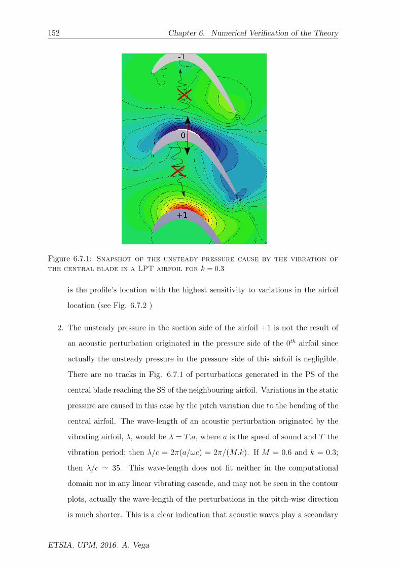
152 Chapter 6. Numerical Verification of the Theory
Figure 6.7.1: Snapshot of the unsteady pressure cause by the vibration ofthe central blade in a LPT airfoil for k = 0.3
is the profile’s location with the highest sensitivity to variations in the airfoil
location (see Fig. 6.7.2 )
2. The unsteady pressure in the suction side of the airfoil +1 is not the result of
an acoustic perturbation originated in the pressure side of the 0th airfoil since
actually the unsteady pressure in the pressure side of this airfoil is negligible.
There are no tracks in Fig. 6.7.1 of perturbations generated in the PS of the
central blade reaching the SS of the neighbouring airfoil. Variations in the static
pressure are caused in this case by the pitch variation due to the bending of the
central airfoil. The wave-length of an acoustic perturbation originated by the
vibrating airfoil, λ, would be λ = T.a, where a is the speed of sound and T the
vibration period; then λ/c = 2π(a/ωc) = 2π/(M.k). If M = 0.6 and k = 0.3;
then λ/c ' 35. This wave-length does not fit neither in the computational
domain nor in any linear vibrating cascade, and may not be seen in the contour
plots, actually the wave-length of the perturbations in the pitch-wise direction
is much shorter. This is a clear indication that acoustic waves play a secondary
ETSIA, UPM, 2016. A. Vega

6.7. Physical Interpretation 153
0 0.5 1
x/c
0
0.5
1
1.5
2
p’/(ρ
eU
e
2δ
/2c)
k=0.3
k=0.03
0
0.5
1
Ise
ntr
op
ic M
ach
Nu
mb
er
Isentropic
Unsteadypressure
Mach
modulus
Unsteady pressuremodulus
Isentropic Mach
(a) (b)
Figure 6.7.2: Isentropic Mach number and unsteady pressure modulusdistributions along blade surface for the: (a) 0th airfoil and (b) +1stairfoil
role in this type of flows.
3. The SS of the central and the +1st airfoil are in first approximation in anti-
phase. When the central blade move downwards (as it happens in the time
instant displayed in Fig. 6.7.1 ) the loading of the SS increases and therefore
the static pressure decreases. The opposite is true for the SS of the -1 airfoil.
4. The basic idea is that the flapping motion of the central airfoil in the y-direction
does not change in first approximation the exit angle of the adjacent passages,
and therefore the total lift of the cascade remains constant. This effectively
means that in a quasi-steady motion if the lift of one of the airfoils increases
the lift of the rest of the airfoils must decrease accordingly, in order that the
global lift remains constant. In this particular mode the balance is obtained
exchanging the lift of the central and +1 airfoil.
All these observations are aligned with the behaviour previously described for the
work-per-cycle as a function of the reduced frequency and the different scaling of the
mean and first harmonic with the frequency. However, to obtain the whole picture it
is necessary to inspect the phasing of the airfoils.
Phase behaviour reveals a number of interesting physical phenomena. At very low
reduced frequencies (k 1) the phase tends either to zero or 180. This is consistent
ETSIA, UPM, 2016. A. Vega
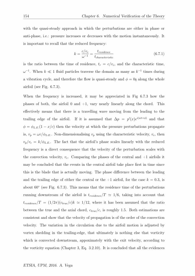
154 Chapter 6. Numerical Verification of the Theory
with the quasi-steady approach in which the perturbations are either in phase or
anti-phase, i.e.: pressure increases or decreases with the motion instantaneously. It
is important to recall that the reduced frequency:
k =c/vcω−1
=tresidence
tcharacteristic(6.7.1)
is the ratio between the time of residence, tr = c/vc, and the characteristic time,
ω−1. When k 1 fluid particles traverse the domain as many as k−1 times during
a vibration cycle, and therefore the flow is quasi-steady and φ = 0ş along the whole
airfoil (see Fig. 6.7.3).
When the frequency is increased, it may be appreciated in Fig 6.7.3 how the
phases of both, the airfoil 0 and +1, vary nearly linearly along the chord. This
effectively means that there is a travelling wave moving from the leading to the
trailing edge of the airfoil. If it is assumed that ∆p = p′(x)ei(wt+φ) and that
φ = φL.E.(1 − x/c) then the velocity at which the pressure perturbations propagate
is, vp = ωc/φL:E.. Non-dimensionalising vp using the characteristic velocity, vc, then
vp/vc = k/φL.E.. The fact that the airfoil’s phase scales linearly with the reduced
frequency is a direct consequence that the velocity of the perturbation scales with
the convection velocity, vc. Comparing the phases of the central and +1 airfoils it
may be concluded that the events in the central airfoil take place first in time since
this is the blade that is actually moving. The phase difference between the leading
and the trailing edge of either the central or the +1 airfoil, for the case k = 0.3, is
about 60 (see Fig. 6.7.3). This means that the residence time of the perturbations
running downstream of the airfoil is tresidence/T ' 1/6, taking into account that
tresidence/T = (1/2π)(ctrue/c)k ' 1/12, where it has been assumed that the ratio
between the true and the axial chord, ctrue/c, is roughly 1.5. Both estimations are
consistent and show that the velocity of propagation is of the order of the convection
velocity. The variation in the circulation due to the airfoil motion is adjusted by
vortex shedding in the trailing-edge, that ultimately is nothing else that vorticity
which is convected downstream, appoximately with the exit velocity, according to
the vorticity equation (Chapter 3, Eq. 3.2.10). It is concluded that all the evidences
ETSIA, UPM, 2016. A. Vega
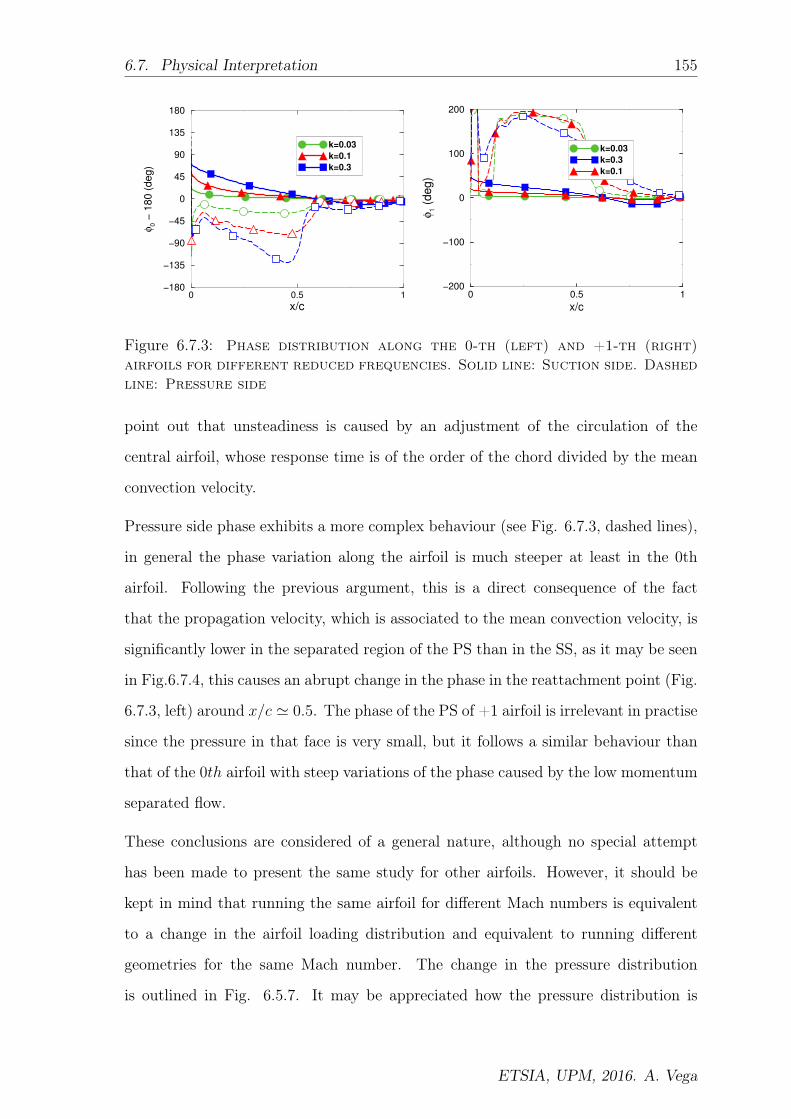
6.7. Physical Interpretation 155
0 0.5 1
x/c
−180
−135
−90
−45
0
45
90
135
180
φ0 −
18
0 (
de
g)
k=0.03
k=0.1
k=0.3
0 0.5 1
x/c
−200
−100
0
100
200
φ1 (
de
g)
k=0.03
k=0.3
k=0.1
Figure 6.7.3: Phase distribution along the 0-th (left) and +1-th (right)airfoils for different reduced frequencies. Solid line: Suction side. Dashedline: Pressure side
point out that unsteadiness is caused by an adjustment of the circulation of the
central airfoil, whose response time is of the order of the chord divided by the mean
convection velocity.
Pressure side phase exhibits a more complex behaviour (see Fig. 6.7.3, dashed lines),
in general the phase variation along the airfoil is much steeper at least in the 0th
airfoil. Following the previous argument, this is a direct consequence of the fact
that the propagation velocity, which is associated to the mean convection velocity, is
significantly lower in the separated region of the PS than in the SS, as it may be seen
in Fig.6.7.4, this causes an abrupt change in the phase in the reattachment point (Fig.
6.7.3, left) around x/c ' 0.5. The phase of the PS of +1 airfoil is irrelevant in practise
since the pressure in that face is very small, but it follows a similar behaviour than
that of the 0th airfoil with steep variations of the phase caused by the low momentum
separated flow.
These conclusions are considered of a general nature, although no special attempt
has been made to present the same study for other airfoils. However, it should be
kept in mind that running the same airfoil for different Mach numbers is equivalent
to a change in the airfoil loading distribution and equivalent to running different
geometries for the same Mach number. The change in the pressure distribution
is outlined in Fig. 6.5.7. It may be appreciated how the pressure distribution is
ETSIA, UPM, 2016. A. Vega

156 Chapter 6. Numerical Verification of the Theory
Figure 6.7.4: Mach number iso-contours and streamlines
significantly aft loaded when the Mach number is increased. The same effect could
be obtained by keeping constant the Mach number and changing the airfoil stagger
angle. This is a clear indication that the conclusions are not linked to a particular
pressure distribution.
6.7.1 Mode-shape variation
It is well known that the sensitivity of the unsteady aerodynamics of vibrating airfoils
to the mode shape is very high [90, 1]. The objective of this section is to understand
how general the physical interpretation presented in the previous section for the flap
mode is. Two more modes have been investigated: the edge-wise mode, represented
as a vibration in the x direction; and a torsion mode about a point located in the
airfoil’s mean line at the maximum thickness location. The same parametric study
that was conducted for the flap mode has been performed for both modes. For the
sake of brevity, just a reduced set of data will be presented here.
6.7.1.1 Edgewise Mode
As we have seen in the previous sections, the conclusions that were drawn for the flap
mode also apply to the edgewise mode. The non dimensional work as a function of
the IBPA and the reduced frequency may be seen in Fig. 6.7.5. It may be appreciated
that, at low reduced frequencies, the damping curves have a sine like shape, which
ETSIA, UPM, 2016. A. Vega

6.7. Physical Interpretation 157
−180 −135 −90 −45 0 45 90 135 180
IBPA
−1
0
1
2
3
4
ΘI=
Wcycle/(
πρ
cU
c
2δ
c
2/2
)
k=0.01
k=0.03
k=0.1
k=0.3
k=0.4
k=0.5
Figure 6.7.5: Non-dimensional work as a function of the IBPA and thereduced frequency for the edge mode
is a direct indication that only the airfoils adjacent to the central contribute to the
work per cycle; however, conversely that in the flap mode, both adjacent airfoils are
equally important (see Fig. 6.7.6, which represent the ratio between the modulus of
the influence coefficients, i.e λ0,−1
λ1).
The trend of the mean value and the first harmonic of the work per cycle with the
reduced frequency is the same as for the flap mode; therefore, they also require the
same differential scaling (see Fig. 6.7.7). It is important to highlight that, to derive
this figure, the contribution of the spikes associated to the resonances have been
removed.
The influence coefficients scale quadratically with the Mach number, whereas the
ratios l1/l0 and l1/l−1 ' 1 are fairly constant with the Mach number and the reduced
frequency, even in a wider range than for the flap mode. Figure 6.7.8 displays the
phases of the zeroth and ±1 airfoils. It may be seen that the phases of all the airfoils
vary linearly with the reduced frequency and the dependence with the Mach number
is very weak but higher than for the flap mode.
The edgewise mode exhibits some differences with respect to the flap mode. Although
the only two significant airfoils from the point of view of the modulus of the pressure
ETSIA, UPM, 2016. A. Vega

158 Chapter 6. Numerical Verification of the Theory
0 0.1 0.2 0.3 0.4
k
0
1
2
3
4
5
λ0,−
1/λ
1
M2=0.6
M2=0.53
M2=0.45
M2=0.33
Figure 6.7.6: Ratio between the modulus of influence coefficient -1,0 and +1as a function of the Reduced frequency and Mach number. Fylled symbols:airfoil -1, empty symbols: airfoil 0
0 0.1 0.2 0.3 0.4 0.5
k
0
0.5
1
1.5
ΘI=
Wcycle/(
πρ
cU
c
2δ
2
c/2
)
Mean value
1st Harmonic
Figure 6.7.7: Mean value and 1st harmonic (variation with the IBPA) of thenon-dimensional work-per-cycle as a function of the reduced frequency forthe edge mode
ETSIA, UPM, 2016. A. Vega

6.7. Physical Interpretation 159
0 0.2 0.4
k
0 0.2 0.4
k
−60
0
60
120
180
φ (
de
g)
M2=0.75
M2=0.6
M2=0.53
M2=0.45
M2=0.33
0 0.2 0.4
k
−60
0
60
120
180
Airfoil −1
Airfoil 0
Airfoil +1
tanα=−2π/180
tanα=1π/180
tanα=−2π/180
Figure 6.7.8: Phases of the zeroth and 1 airfoils (filled symbols), and −1airfoil (solid symbols) as a function of k and M .
perturbation in the flap mode, the zeroth and the positive-first airfoils, are dominated
by vorticity waves, and are therefore fairly insensitive to Mach number variations,
the zeroth and negative-first airfoils of the edgewise mode show a weak sensitivity
to the Mach number. This presence of acoustic waves helps to explain why the
suction side of the zeroth and the pressure side of the negative-first airfoil are in anti-
phase for any Mach number and reduced frequency (note that, in Fig. 6.7.8, φ0 − k
departs from 0 deg, whereas the φ−1 − k departs from π). This is only possible if
the effective velocity of propagation (the sound speed) is much larger, and therefore
both surfaces are synchronised at any instant and flow condition. Vorticity waves,
superimposed with the aforementioned acoustic waves, may also be seen in the zeroth
airfoil; however, the precise contribution of each of them cannot be done without a
proper mode decomposition.
The influence of acoustic waves in the edgewise mode may also be appreciated in the
work-per-cycle curves (Fig. 6.7.5), where the spikes associated to the inlet and outlet
resonance conditions may be seen. This is only possible if the pressure perturbations
associated to the acoustic waves are at least of the same order as those associated
to the vorticity waves. Note that, under the same conditions, these spikes are not
ETSIA, UPM, 2016. A. Vega

160 Chapter 6. Numerical Verification of the Theory
−180 −135 −90 −45 0 45 90 135 180
IBPA
−0.5
0
0.5
1
1.5
2
ΘI=
Wcycle/(
πρ
c
2
δc
2U
c
2/2
)
M2=0.185 (k=0.3)
M2=0.5 (k=0.3)
M2=0.6 (k=0.3)
M2=0.6 (k=0.03)
Figure 6.7.9: Non-dimensional work as a function of the IBPA and the Machnumber for the edgewise mode.
visible in the flap mode; that is solely controlled by vortex shedding mechanisms.
Although the resonance conditions are mode independent, their excitation is not,
which is the ultimate reason why these are clearly seen in some modes while not
in others. Acoustic resonances require excitement by an acoustic mode that is not
present in the flex mode, which is the contrary to the edgewise mode. In any case, the
sensitivity to the Mach number is low, especially at the lowest reduced frequencies.
Figure 6.7.9 displays the dependence of the non dimensional aerodynamic work per
cycle with the Mach number. It may be appreciated that all the curves collapse in
a single but, in this case, conversely that in the flap mode, a slight dependence with
M2 exists, since the phase of the ICs exhibits a weak dependence with M2 (see Fig.
6.7.8). Summarising, the functional form for Wcycle [Eq. 6.5.4] derived for the flex
mode is still valid, although its ability to retain the variation with the Mach number
is smaller. The constants of the model for this mode are obviously different, and it
has to be recalled that, in this case, the ratio l−1/l1 needs to be retained because it
is not negligible.
ETSIA, UPM, 2016. A. Vega

6.7. Physical Interpretation 161
−180 −135 −90 −45 0 45 90 135 180
IBPA
−2
0
2
4
6
ΘI=
Wcycle/(
πρ
cU
c
2δ
2
c/2
)
k=0.02
k=0.03
k=0.1
k=0.3
k=0.4
k=0.5
Figure 6.7.10: Non-dimensional work as a function of the IBPA and thereduced frequency for the torsion mode.
6.7.1.2 Torsion Mode
This torsion mode (which represents a torsion about the midpoint of the airfoil) is
more difficult to interpret than the flap and edgewise modes. The effort here will be
concentrated on describing just the main differences that may be summarised in the
following two observations. The first is that the contribution to the work per cycle
of the 2 airfoils far away to the vibrating one is relevant. This may be concluded by
just realising that the work per cycle as a function of the IBPA is a discontinuous
sawtooth function (see Fig. 6.7.10) with a rich harmonic content.
Figure 6.7.11 displays the moment influence coefficients, and it may be appreciated
that the contribution of airfoils far away from the central one is still significant, and
that the moment influence coefficient of the blade i on the blade zeroth, li, is li ∝ 1/i,
as corresponds to the Fourier coefficients of a sawtooth function.
It may be seen (Fig. 6.7.12) that the modulus of the unsteady pressure in the
zeroth and the negative-first airfoil is much larger than that of the rest of the airfoils.
However, due to the torsion nature of the motion, the unsteady pressure contribution
to the moment of the front and rear parts of the airfoil cancels out, giving rise to a
ETSIA, UPM, 2016. A. Vega

162 Chapter 6. Numerical Verification of the Theory
−5 −3 −1 1 3 5
Airfoil Index
0
0.2
0.4
0.6
0.8
m0=
f 0/0
.5ρ
cU
c
2δ
cc
k=0.03
k=0.3
Figure 6.7.11: Non-dimensional moment influence coefficients of the torsionmode at two different reduced frequencies and M2 = 0.75.
relatively low contribution of these airfoils. On the contrary, −2, −3, and −4 have a
relatively small unsteady pressure in the trailing-edge region that is amplified when
the moment with respect to the central part of the airfoil is computed. The same is
true for 2, 3, and 4 airfoils but with the leading- edge region.
The torsion mode motion, contrary to the flap and edgewise modes, changes the exit
angle, and therefore the lift of the cascade. The system reacts, creating upstream
running pressure waves departing from the domain exit, that can be clearly seen
in the simulations. When the exit angle of the central airfoil is changed, the whole
cascade reacts, adjusting the mass flow. This information is transmitted upstream by
means of pressure waves. It may be seen in Fig. 6.7.13 how the phase of the central
airfoil is independent of the Mach number; this means that the unsteady pressure is
controlled by vortex shedding. However, the phases of the rest of the airfoils, in anti-
phase with the central one, vary with the Mach number, which is a clear indication
that they are dominated by acoustic waves.
The second difference is that the Mach number sensitivity of the 2 and 1 airfoil phases
is noticeable; therefore, the sensitivity of the non dimensional work per cycle to the
Mach number is higher than for the flap mode, where φi remains unaltered with M
ETSIA, UPM, 2016. A. Vega
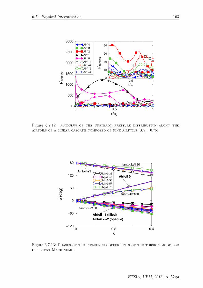
6.7. Physical Interpretation 163
0 0.5 1
x/cx
0
40
80
120
160
p’ T
OR
SIO
N
0 0.5 1
x/cx
0
500
1000
1500
2000
2500
3000
p’ T
OR
SIO
N
Airf 4
Airf 3
Airf 2
Airf 1
Airf 0
Airf −1
Airf −2
Airf −3
Airf −4
Figure 6.7.12: Modulus of the unsteady pressure distribution along theairfoils of a linear cascade composed of nine airfoils (M2 = 0.75).
0 0.2 0.4
k
−120
−60
0
60
120
180
φ (
de
g)
M2=0.33
M2=0.45
M2=0.53
M2=0.57
M2=0.75
Airfoil −1 (filled)
Airfoil 0
Airfoil +1
tanα=4π/180
tanα=2π/180
tanα=2π/180
Airfoil +/−2 (opaque)
Figure 6.7.13: Phases of the influence coefficients of the torsion mode fordifferent Mach numbers.
ETSIA, UPM, 2016. A. Vega

164 Chapter 6. Numerical Verification of the Theory
but lower than for the edge mode, where φ0 and φ1 vary with the Mach number. The
Mach number sensitivity of the airfoils located far away from the central, and which
are dominated by the acoustic waves, is a general trend for all the modes, but is only
relevant for the torsion mode. Moreover, the reduced-frequency range for which the
phase trend is linear with k is narrower. As a consequence, the work-per-cycle model
described in Eq. 6.5.2 needs to be extended to include more ICs and to take into
account Mach number effects.
6.8 Conclusions of the Numerical Validation
All the theoretically derived conclusions have been numerically verified using a well-
validated linearised Navier–Stokes solver on a multiplicity of two-dimensional airfoils
operating at design/off-design and high subsonic/transonic conditions, vibrating
with different mode-shapes. Both the travelling-wave and the influence coefficient
techniques have been used, showing consistent results. The numerical study has
been focused on the behaviour of the bending mode but a some results for the
three fundamental modes have also been shown to prove that the conclusions are
independent of the mode- shape.
The unsteady aerodynamics of vibrating airfoils and its impact on the work-per-cycle
curves in the low reduced frequency regime has been analytically studied by means
of a new non-dimensional airfoil unsteady loading parameter (ULP). It has been
proved my means of numerical experiments that by using the ULP to characterise
the loading it is possible to correlate the different trends with the reduced frequency
of the influence coefficient moduli, the IC phases, and the work-per-cycle curves in a
quantitative manner.
The main conclusions for airfoils oscillating at low reduced frequency are the following:
1. The unsteady aerodynamic loading parameter (ULP) is able to predict and to
quantify the behaviour of the influence coefficient modulus and phase (and then
ETSIA, UPM, 2016. A. Vega
6.8. Conclusions of the Numerical Validation 165
of the stability trends of the work per cycle curves) to changes in the operating
conditions, mode-shape and (in a qualitative way) airfoil geometry.
2. The sign of the ULP predicts, from the point of view of the influence coefficient
technique, which of the adjacent airfoils has the highest contribution to the work
per cycle, i.e. which airfoil has the highest unsteady pressure. This fact has a
direct implication on the sign of IBPA where the minimum damping occurs.
3. High ULP values implies that the theory is valid for a wide range of reduced
frequencies, while small values lead to a more restricted range.
4. The ULP can be used to quantitatively predict the influence of different
aerodynamic loadings, reduced frequency and mode-shapes in the aerodynamic
damping, not only for a given airfoil geometry, but also to establish qualitative
comparisons among different airfoils.
5. The unsteady pressure in the flap mode is caused mainly by convective vorticity
modes in the central and adjacent airfoils. Acoustic perturbations do not play
any role in the low reduced- frequency regime. This is supported by the fact
that the phases of the influence coefficients are fairly independent of the Mach
number, although their moduli scale with the Mach number. The linear increase
of the phase with the reduced frequency is a direct consequence of the convective
nature of the unsteady perturbations.
6. The effect of the Mach number on the flap mode is a pure scaling of the damping
curves; therefore, it does not change the stability region but instead changes the
severity of the instability, that increases with the Mach number. The scaling of
the Mach number is directly absorbed by the non-dimensionalisation.
7. The physical behaviour of the flap mode is different for the edgewise and
torsion modes. The edgewise mode shows a weak dependence with the Mach
number, whereas for the torsion mode, the contribution of more ICs is needed
to reconstruct the work per cycle.
ETSIA, UPM, 2016. A. Vega
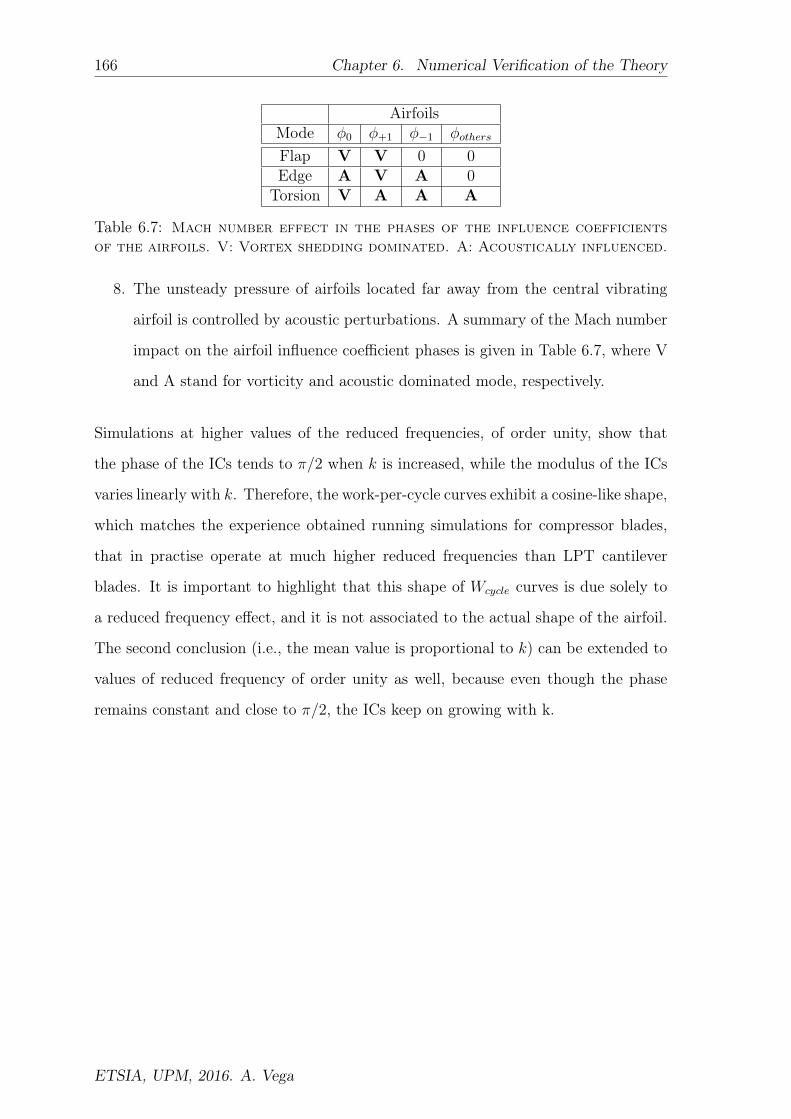
166 Chapter 6. Numerical Verification of the Theory
AirfoilsMode φ0 φ+1 φ−1 φothers
Flap V V 0 0Edge A V A 0
Torsion V A A A
Table 6.7: Mach number effect in the phases of the influence coefficientsof the airfoils. V: Vortex shedding dominated. A: Acoustically influenced.
8. The unsteady pressure of airfoils located far away from the central vibrating
airfoil is controlled by acoustic perturbations. A summary of the Mach number
impact on the airfoil influence coefficient phases is given in Table 6.7, where V
and A stand for vorticity and acoustic dominated mode, respectively.
Simulations at higher values of the reduced frequencies, of order unity, show that
the phase of the ICs tends to π/2 when k is increased, while the modulus of the ICs
varies linearly with k. Therefore, the work-per-cycle curves exhibit a cosine-like shape,
which matches the experience obtained running simulations for compressor blades,
that in practise operate at much higher reduced frequencies than LPT cantilever
blades. It is important to highlight that this shape of Wcycle curves is due solely to
a reduced frequency effect, and it is not associated to the actual shape of the airfoil.
The second conclusion (i.e., the mean value is proportional to k) can be extended to
values of reduced frequency of order unity as well, because even though the phase
remains constant and close to π/2, the ICs keep on growing with k.
ETSIA, UPM, 2016. A. Vega

Chapter 7
Stabilisation Mechanism of Blade
Pairs: Numerical and Experimental
Evidences
If everyone is thinking alike, then
somebody isn’t thinking
G. S. Patton
Contents
7.1 Context and Problem Description . . . . . . . . . . . . . 167
7.2 Experimental Setup . . . . . . . . . . . . . . . . . . . . . . 170
7.3 Numerical Validation . . . . . . . . . . . . . . . . . . . . . 174
7.4 Discussion of the Stabilisation Mechanism . . . . . . . . 181
7.5 Concluding Remarks . . . . . . . . . . . . . . . . . . . . . 183
7.1 Context and Problem Description
As it has been already mentioned in the introduction, modern Low Pressure Turbine
(LPT) bladed-disk are made up of very slender rotor blades, and fluter prone. The
167

168 Chapter 7. Stabilisation Mechanism of Welded-in-Pair
Cantilever
Interlock
Welded−pair
(a)Cantilever (b) Interlock
(c)Welded-pair
Figure 7.1.1: Layout of different bladed-disc assembly configurations
capability of control their vibration is a major engineering issue. In order to control
the vibration of shrouded LPT rotor blades, three different configurations have been
taken into consideration along the history: cantilever, interlock and welded in pair
configurations. Figure 7.1.1 (top) represents a sketch of the shrouds of the three
configurations, whereas a global view of the whole assembly can be seen in bottom
of the same figure.
The main problem of cantilever blades is that, as long as flat sided shrouds can vibrate
freely, even for very small clearances, and especially for low inter-blade phase angles
(IBPA), they provide little control over the vibration characteristics of bladed-disks.
As an alternative, interlock configurations (consisting on z-shaped shrouds in contact
with the neighbouring airfoils) were designed with the aim of remain tight during the
whole flight envelope. This design significantly modifies the vibration characteristics
of cantilever blades, introducing three new problems, namely, the coupling between
the bending and torsion, giving rise to complex modes, the high sensitivity of mode-
ETSIA, UPM, 2016. A. Vega

7.1. Context and Problem Description 169
shapes and natural frequencies to the details of the contact region, and finally the
difficulty in evaluating the frequency characteristics along the engine life due to the
deterioration of the contact surfaces. As a consequence of the limitations of both, the
cantilever and the interlock configurations, pairs of blades welded in the tip-shroud
(see Fig. 7.1.2) were introduced as a practical alternative to control the vibration
characteristics of LPT bladed-discs, and can be observed in many large civil turbofan
engines.
This latter configuration substantially modifies the mode-shapes and eigenfrequencies
of the cantilever and interlock configurations. The influence of blade mode-shape
and reduced frequency on the flutter boundaries of LPTs has been numerically studied
[90] and supported by experiments [5] in the past. The beneficial effect of grouping
the airfoils in pairs was firstly demonstrated by Whitehead and Evans [102]. Kahl
[103] studied the stability of a LPT sectored vane of three airfoils, and later on
Chernysheva [104] extended it to a packet of six vanes using the Panovsky and Kielb
(PK) method. More recently, Corral et al. [1] studied the influence of pairing the
rotor blades on the aerodynamic damping of a typical LPT bladed-disc, and compared
the results with the equivalent interlock configuration. Moreover it has been shown
that the potencial beneficial effect of grouping the blades in sectored vanes is mostly
spoiled due to structural coupling [2, 105]. Finally, the unsteady aerodynamics of
blade clusters has been recently investigated experimentally [106].
In this conext, the main motivation of this chapter is twofold. Firstly, to validate
and explain the working principles of the welded-in-pair configuration, combining
experimental data obtained at the EPFL non-rotating annular test facility, and
new numerical simulations; and secondly, to serve as an indication of the level of
accuracy that can be obtained with the linearised code used in this thesis. Both, the
experiments and the simulations were conducted in the framework of the european
project FUTURE, that funded my work during three years. This is the ultimate
reason of include this chapter in the thesis.
The stabilization mechanism by means of welding the rotor blades in pairs had been
ETSIA, UPM, 2016. A. Vega

170 Chapter 7. Stabilisation Mechanism of Welded-in-Pair
Figure 7.1.2: 1st flap mode-shape of a welded-in-pair rotor blade configura-tion
previously described recurring solely to analytical methods [1]. Here these studies
are extended using recently available experimental data. The numerical simulations
have been performed by means of a well validated linearized Navier-Stokes solver,
known as Mu2s2T −L, described in the chapter “Analytical and Numerical Models”.
7.2 Experimental Setup
The experimental data used for the validation of the numerical simulations was
obtained in a dedicated experimental campaing performed at the Ecole Polytechnique
Fédérale de Lausanne (EPFL). The test facility consists on a non-rotating annular
cascade, presented by Bölcs [107]. This facility allows steady and unsteady testing
of both, compressor and turbine rotor cascades, in several subsonic, transonic and
supersonic flow conditions, with a large variation of inlet flow angles. The incoming
air is swirled while the rotor cascades are at rest, obtaining in this way the same
relative flow conditions as in a real turbomachinery. This original concept is achieved
with the use of a radial-axial nozzle in combination with variable pitch pre-swirl
vanes, as schematically represented in Fig. 7.2.1, on the left. The main advantage of
this non-rotating setup is the ease of measurement and data acquisition, the direct
optical access and the possibility of using extensive measurement equipment and
controls without the use of costly telemetry systems.
ETSIA, UPM, 2016. A. Vega

7.2. Experimental Setup 171
(a) (b)
Figure 7.2.1: Schematic view of the non rotating annular test facility (a)and turbine rotor cascade instrumentation, view from downstream side (b)
7.2.1 Test Facility
A 2.25 MW four-stage centrifugal compressor supplies the test facility with
compressed air in an open loop. The air exiting the compressor is cooled by two
heat exchangers which allow to adjust the air temperature entering the test facility.
Figure 7.2.1 (a) represents the test facility and it can be seen that the incoming air
in the radial direction (1,2) is pre-swirled by two sets of pre-swirl vanes (5,6), before
accelerating and turning in an axial direction in the radial-axial nozzle. At this
point, the flow approaches the test section (7). Afterwards, the flow turns in a radial
direction and exits (12) the test facility. With this setup, a quasi-two-dimensional
flow at mid-channel height in the test section can be achieved. The flow quantities
(total pressure, outlet static pressure and inlet flow angle) can be adjusted via the
inlet (1,2) and outlet (12) valves and the pre-swirl vanes (5,6). The total temperature
of the flow at inlet is measured in the upstream settling chamber (3,4).
The measuring cascade, represented in Fig. 7.2.1 (b), is composed by twenty prismatic
turbine blades, each one has its own independent suspension system for controlled
vibration, as shown in Fig. 7.2.2, on the left. The modular blade suspension system
setup facilitates the potential change or reposition of components.
The blade vibration frequency is controlled by the stiffness of a spring integrally
ETSIA, UPM, 2016. A. Vega

172 Chapter 7. Stabilisation Mechanism of Welded-in-Pair
machined with the airfoil and the rest of the suspension system. The airfoil
mode-shape is controlled by the shape of the spring, which is nothing else than a
relatively thin and flexible part of the bar, either bending or torsion modes can be
accommodated. Since the stiffness of the spring is much lower than that of the rest
of the system, the mode-shape displacements in the airfoil region correspond in first
approximation to a rigid body motion, and vary linearly from hub to tip.
Only vibration in one translation direction is enabled. Each individual blade system
is oscillated by means of electromagnets with an independent vibration amplitude
and phase, whereas the vibration frequency is the same for all blades. The vibration
frequency has to be close to the natural frequency of the modular blade suspension
systems. The displacement in each blade is controlled by means of an inductive
proximity transducer.
The steady state flow-field is determined by means of aerodynamic 5-hole L-shaped
probes located at upstream and downstream positions of the measuring rotor cascade.
Figure 7.2.2, on the right, represents the traversing locations of each probe with
respect to the leading and trailing edges. Two probe holders together with two precise
industrial linear displacement systems allow controlling the radial position of each
probe. Each probe is staggered along the mean flow direction at the corresponding
flow measuring location. The combination of the radial positioning of the probes and
the rotation indexing of the measuring cascade allows precise flow mapping of the
in- and outflow conditions. One measurement per degree is taken in circumferential
direction for 18ş in total to cover one pitch of a cascade built by 20 blades, and 14
measurement positions are taken along the channel height.
Six blades are equipped with steady-state pressure taps in order to measure the static
surface pressure. These taps are located at three different blade heights (25%, 50%
and 90%), as pairs of PS and SS measuring blades (see Fig. 7.2.1, on the right),
allowing in this way the validation of the quasi-two-dimensional flow assumption as
well as the computation of the steady loading. There are twelve measuring locations
on the SS measuring blades and nine measuring locations on the neighboring PS
ETSIA, UPM, 2016. A. Vega

7.2. Experimental Setup 173
Figure 7.2.2: Blade suspension system (left) and Probe traverse locations(right)
measuring blades with an identical LE measurement location on both blades, that
can be seen on Fig. 7.2.2, (right). This is useful to verify the symmetry of the
incoming flow (angle of attack), as the PS and SS transducers are not located on the
same blade, resulting in a channel measurement in a blade passage.
The unsteady flow field is measured by means of cylindrical high response piezo-
resistive absolute pressure transducers, mounted in the blades at mid-channel height
at the same locations as the steady pressure taps, but in different blades, allowing
the measurement of the pressure fluctuations on the blade surface.
The acquisition technique used at EPFL enables to record the blade displacement and
the unsteady pressures simultaneously, which allows to determine the aerodynamic
blade damping. Taking into account the possibilities of the electromagnetic vibration
system and the aforementioned measurement options, all possible inter-blade phase
angles (IBPA) can be investigated.
Furthermore, the characteristics of the facility allow the investigation of packet
of blades by setting the vibration amplitude and phase of the neighboring blades
accordingly.
ETSIA, UPM, 2016. A. Vega

174 Chapter 7. Stabilisation Mechanism of Welded-in-Pair
7.3 Numerical Validation
7.3.1 Problem Description
The mode-shapes of the first modes of a LPT welded-in-pair rotor blade can be
described in first approximation as pairs of airfoils vibrating in phase, whose two-
dimensional sections are undeformed and can be considered as two-dimensional rigid
bodies (see Fig. 7.1.2). These mode-shapes, typical of high aspect ratio rotor blades
are well suited to be represented in the EPFL annular cascade, whose airfoils are
vibrated as rigid bodies with an individual control of the blade phase.
The EPFL annular vibrating cascade provides a large degree of flexibility to
implement different types of modes, since the amplitude and phase of each airfoil
can be selected independently while having a constant vibration frequency for all
airfoils.
To investigate the damping associated to the welded-in-pair configurations, first of
all the bending and torsion mode of the corresponding cantilever configuration have
been reproduced in the test facility, by vibrating all airfoils with an identical angular
frequency, ω, amplitude, δ, and IBPA. To represent the mode-shapes of the welded-
in-pair configuration a basic sector of two blades instead of one is chosen. Inside the
pair, the two airfoils move in phase with the same amplitude, while all pairs move
with the same angular frequency, ω, and Inter-sector Sector Phase Angle (ISPA).
The IBPA represents the phasing between neighboring blades, and is commonly
defined as σ = 2πm/Ns, wherem = 0, ...,±Ns/2 andNs is the number of fundamental
sectors. According with the previous definition, Ns = Nb for the single blade case,
where Nb represents the number of blades, and for the welded in pair configuration
Ns = Nb/2 . Therefore the number of Inter Sector Phase Angles (ISPA) is half of
the number of possible IBPAs. In the convention used in this thesis a positive IBPA
physically means a forward traveling-wave. i.e.; a wave moving in the same direction
than the rotor.
The most unstable modes of a high aspect ratio cantilever low-pressure turbine are
ETSIA, UPM, 2016. A. Vega

7.3. Numerical Validation 175
Torsion
Bending
Figure 7.3.1: Bending direction and torsion axis
the first bending and torsion modes. The frequency and mode-shape of the bending
mode are fairly unaffected by welding the blades in pairs [1], however the torsion
mode lowers slightly its frequency and the torsion center of the airfoil is moved from
the mid-chord to about the center of the passage.
Traveling wave mode experiments for a packet of two blades and for a single blade,
both performing an oscillation in a bending direction orthogonal to the blade chord,
representing the first flap mode, and a torsion about the z-axis have been considered.
Figure 7.3.1 represents the position of the bending axis with respect to the blade
chord and the position of the torsion axis. All possible Inter Sector Phase Angles
(ISPA) for the packet configuration, and all the possible Inter Blade Phase Angles
for the single blade configuration have been considered.
As it has been mentioned before, due to the design of the airfoil mounting system,
the displacements on the airfoil correspond to a rigid body motion, which is a good
description of the mode-shape in a two-dimensional section of a high aspect ratio
airfoil. The selection of the mode-shape of the pair is fully justified for the bending
mode, where the motion of each individual airfoil of the packet is very similar in
practice to that of the single airfoil.
The mode-shape of the torsion mode is less justified since both airfoils should have a
common torsion center located around the midle of the passage. To properly represent
ETSIA, UPM, 2016. A. Vega
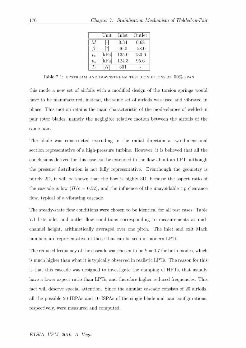
176 Chapter 7. Stabilisation Mechanism of Welded-in-Pair
Unit Inlet OutletM [-] 0.34 0.68β [] 46.0 -58.0pt [kPa] 135.0 130.6ps [kPa] 124.3 95.6Tt [K] 301 -
Table 7.1: upstream and downstream test conditions at 50% span
this mode a new set of airfoils with a modified design of the torsion springs would
have to be manufactured; instead, the same set of airfoils was used and vibrated in
phase. This motion retains the main characteristic of the mode-shapes of welded-in
pair rotor blades, namely the negligible relative motion between the airfoils of the
same pair.
The blade was constructed extruding in the radial direction a two-dimensional
section representative of a high-pressure turbine. However, it is believed that all the
conclusions derived for this case can be extended to the flow about an LPT, although
the pressure distribution is not fully representative. Eventhough the geometry is
purely 2D, it will be shown that the flow is highly 3D, because the aspect ratio of
the cascade is low (H/c = 0.52), and the influence of the unavoidable tip clearance
flow, typical of a vibrating cascade.
The steady-state flow conditions were chosen to be identical for all test cases. Table
7.1 lists inlet and outlet flow conditions corresponding to measurements at mid-
channel height, arithmetically averaged over one pitch. The inlet and exit Mach
numbers are representative of those that can be seen in modern LPTs.
The reduced frequency of the cascade was chosen to be k = 0.7 for both modes, which
is much higher than what it is typically observed in realistic LPTs. The reason for this
is that this cascade was designed to investigate the damping of HPTs, that usually
have a lower aspect ratio than LPTs, and therefore higher reduced frequencies. This
fact will deserve special attention. Since the annular cascade consists of 20 airfoils,
all the possible 20 IBPAs and 10 ISPAs of the single blade and pair configurations,
respectively, were measured and computed.
ETSIA, UPM, 2016. A. Vega
7.3. Numerical Validation 177
7.3.2 Results
7.3.2.1 Work-per-Cycle Computation
The work-per-cycle, Wcycle, of the airfoil is usually presented in non-dimensional form
according to the following formula:
Θ1 =Wcycle
12ρcv2
cδ2H
(7.3.1)
where Wcycle is the work per cycle over the blade, ρc and vc are, respectively, the
density and velocity at the cascade inlet, δ is the maximum airfoil displacement, and
H is the blade height. It is assumed that the characteristic unsteady pressure is a
fraction of the inlet dynamic head, i.e.: pc−unsteady = 12ρcv
2cδcand the characteristic
surface S = H c, where c is the airforil chord.
In the present study the work-per-cycle has been computed in a different way in the
experiments than in the simulations. Since the cascade airfoils are equipped with
unsteady pressure transducers only in the mid-section of the airfoil, therefore only
the unsteady pressure corresponding to the mid-section has been used to compute
the Wcycle, whereas for the simulations the entire airfoil surface has been employed.
The work-per-cycle for a packet of blades is computed considering the aerodynamic
surfaces of all the airfoils, and then normalizing the result by the number of airfoils
in the packet, two in this case, to allow a comparison of the results with the single
blade case.
7.3.2.2 Steady State Results
The annular cascade consists of 20 airfoils with an aspect ratio H/c = 0.52 and
a relative tip gap g/c = 0.7%. The cascade exhibits an inter-platform gap in the
platforms to allow the blades to vibrate freely, resulting in the presence of a small
leakage in the hub region.
A semi-unstructured grid with 25 radial planes and 370,000 points was created. No
provision was made neither for the tip-clearance nor for the inter-platform gaps, but
ETSIA, UPM, 2016. A. Vega
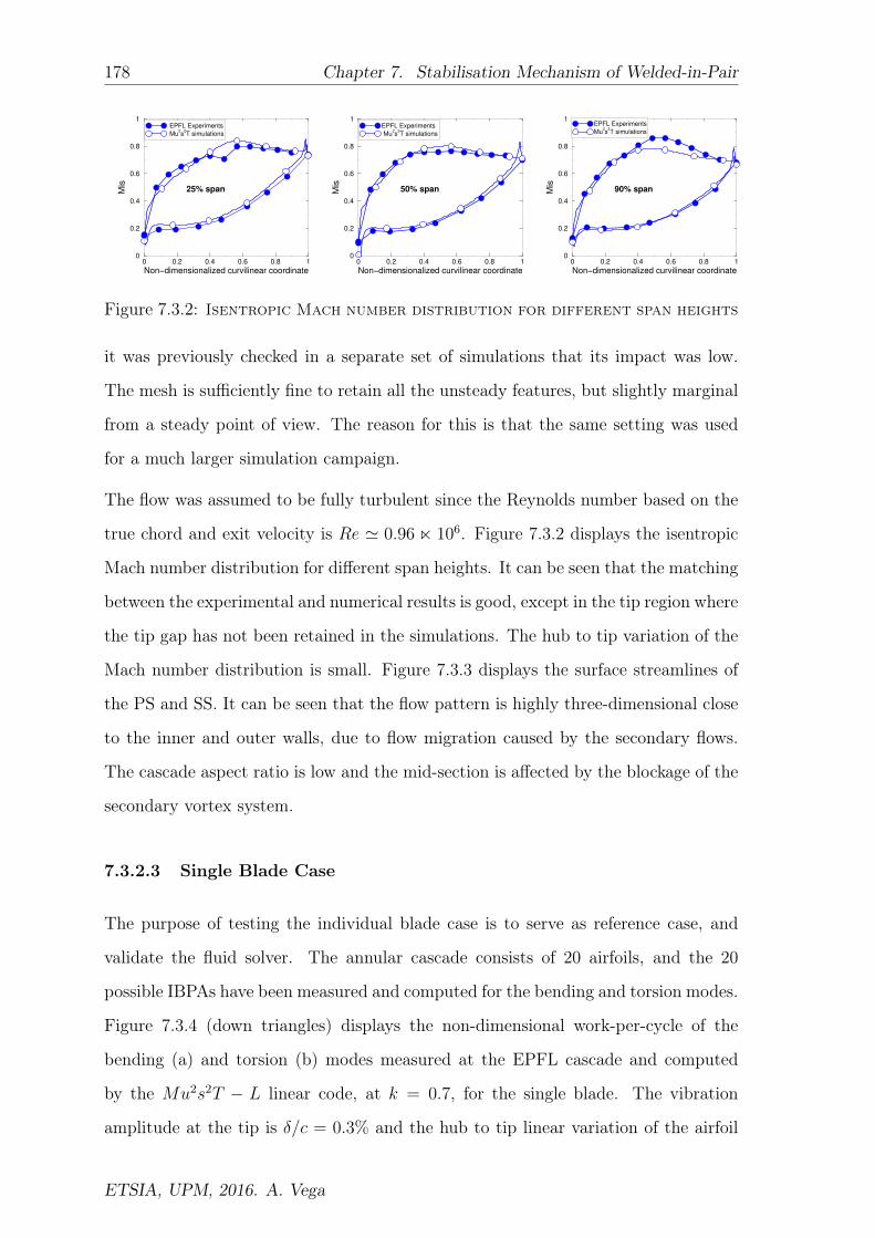
178 Chapter 7. Stabilisation Mechanism of Welded-in-Pair
0 0.2 0.4 0.6 0.8 1
Non−dimensionalized curvilinear coordinate
0
0.2
0.4
0.6
0.8
1M
is EPFL Experiments
Mu2s
2T simulations
25% span
0 0.2 0.4 0.6 0.8 1
Non−dimensionalized curvilinear coordinate
0
0.2
0.4
0.6
0.8
1
Mis
EPFL Experiments
Mu2s
2T simulations
50% span
0 0.2 0.4 0.6 0.8 1
Non−dimensionalized curvilinear coordinate
0
0.2
0.4
0.6
0.8
1
Mis
EPFL Experiments
Mu2s
2T simulations
90% span
Figure 7.3.2: Isentropic Mach number distribution for different span heights
it was previously checked in a separate set of simulations that its impact was low.
The mesh is sufficiently fine to retain all the unsteady features, but slightly marginal
from a steady point of view. The reason for this is that the same setting was used
for a much larger simulation campaign.
The flow was assumed to be fully turbulent since the Reynolds number based on the
true chord and exit velocity is Re ' 0.96 n 106. Figure 7.3.2 displays the isentropic
Mach number distribution for different span heights. It can be seen that the matching
between the experimental and numerical results is good, except in the tip region where
the tip gap has not been retained in the simulations. The hub to tip variation of the
Mach number distribution is small. Figure 7.3.3 displays the surface streamlines of
the PS and SS. It can be seen that the flow pattern is highly three-dimensional close
to the inner and outer walls, due to flow migration caused by the secondary flows.
The cascade aspect ratio is low and the mid-section is affected by the blockage of the
secondary vortex system.
7.3.2.3 Single Blade Case
The purpose of testing the individual blade case is to serve as reference case, and
validate the fluid solver. The annular cascade consists of 20 airfoils, and the 20
possible IBPAs have been measured and computed for the bending and torsion modes.
Figure 7.3.4 (down triangles) displays the non-dimensional work-per-cycle of the
bending (a) and torsion (b) modes measured at the EPFL cascade and computed
by the Mu2s2T − L linear code, at k = 0.7, for the single blade. The vibration
amplitude at the tip is δ/c = 0.3% and the hub to tip linear variation of the airfoil
ETSIA, UPM, 2016. A. Vega
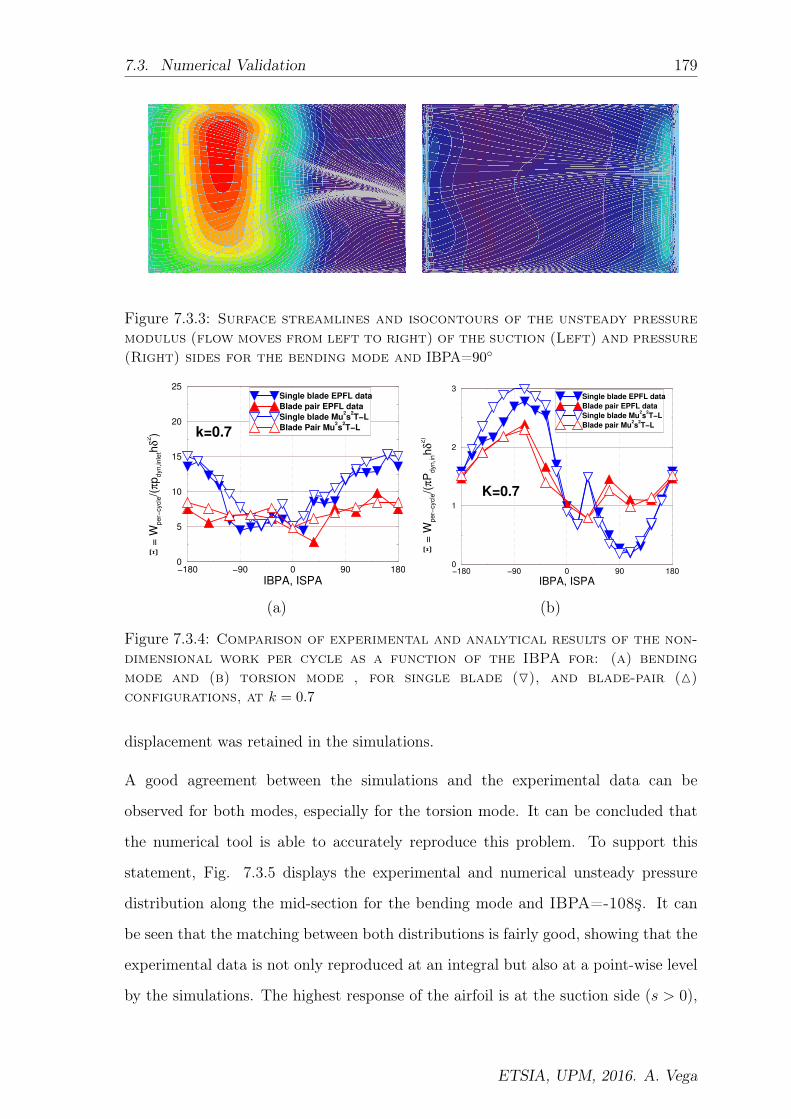
7.3. Numerical Validation 179
Figure 7.3.3: Surface streamlines and isocontours of the unsteady pressuremodulus (flow moves from left to right) of the suction (Left) and pressure(Right) sides for the bending mode and IBPA=90
−180 −90 0 90 180
IBPA, ISPA
0
5
10
15
20
25
Ξ =
Wper−
cycle/(
πp
dyn,inle
thδ
2)
Single blade EPFL data
Blade pair EPFL data
Single blade Mu2
s2
T−L
Blade Pair Mu2
s2
T−Lk=0.7
−180 −90 0 90 180
IBPA, ISPA
0
1
2
3
Ξ =
Wp
er−
cycle/(
πP
dyn
,inh
δ2
)
Single blade EPFL data
Blade pair EPFL data
Single blade Mu2
s2
T−L
Blade pair Mu2
s2
T−L
K=0.7
(a) (b)
Figure 7.3.4: Comparison of experimental and analytical results of the non-dimensional work per cycle as a function of the IBPA for: (a) bendingmode and (b) torsion mode , for single blade (O), and blade-pair (M)configurations, at k = 0.7
displacement was retained in the simulations.
A good agreement between the simulations and the experimental data can be
observed for both modes, especially for the torsion mode. It can be concluded that
the numerical tool is able to accurately reproduce this problem. To support this
statement, Fig. 7.3.5 displays the experimental and numerical unsteady pressure
distribution along the mid-section for the bending mode and IBPA=-108ş. It can
be seen that the matching between both distributions is fairly good, showing that the
experimental data is not only reproduced at an integral but also at a point-wise level
by the simulations. The highest response of the airfoil is at the suction side (s > 0),
ETSIA, UPM, 2016. A. Vega

180 Chapter 7. Stabilisation Mechanism of Welded-in-Pair
−1 0 10
0.5
1
1.5
2
p’/(p
dynδ/c
)
1st blade EPFL data
2nd
blade EPFL data
1st blade Mu
2s
2T−L
2nd
blade Mu2s
2T−L
−1 0 1
s
0
0.5
1
1.5
2
p’/(p
dynδ/c
)
SB EPFL data
SB Mu2s
2T−L
IBPA,ISPA= −108
Figure 7.3.5: Experimental (filled symbols) and numerical (opaque symbols)unsteady pressure modulus distribution along the blade chord for singleblade and blade pair package configurations for IBPA=-108ş and ISPA=-108,respectively at k = 0.7 for a bending motion
in the peak Mach number region, as it could be expected. The unsteady pressure
level at the pressure side (s < 0) is much lower, and therefore it can be concluded
that the major contribution to the Wcycle is due to the airfoil SS.
Figure 7.3.3 shows that, although the flow is highly three-dimensional, the unsteady
pressure variation in the spanwise direction is small. Hence a section by section
investigation of the unsteady pressure is applicable, analogously as for a high aspect
ratio LPT rotor blade.
7.3.2.4 Welded-Pair Case
In order to experimentally verify the effect of welding the rotor blades in pairs, the
same blades for the same steady boundary conditions were vibrated in bending and
torsion, forcing that the pair of airfoils vibrate in phase. Since the cascade can contain
only 10 pairs, 10 ISPA were measured and computed.
Figure 7.3.4 (a) and (b) (up triangles) display the work-per-cycle measured at the
EPFL cascade and computed by the Mu²s²T − L linear code, at k = 0.7, for the
bending (a) and the torsion (b) modes. The first observation is that the overall
damping of the system is lower than that of the single blade configuration. This is
ETSIA, UPM, 2016. A. Vega

7.4. Discussion of the Stabilisation Mechanism 181
(a) (b)
Figure 7.3.6: Unsteady pressure modulus obtained from the simulations forthe torsion mode at k = 0.7. IBPA/ISPA=180ş. (a) single blade configurationand (b) pair configuration
due to the reduced level of activity on the SS of the airfoil 2 of the pair (the one
that has its SS in the pair passage). The effect is bigger for the largest ISPAs, that
have as well a higher relative movement of the blades, while the vicinity of IBPA=0
is unaffected by the pair configuration.
It can be concluded that the numerical method is able to reproduce the experimental
data, including the decrease in the unsteady pressure field of the 2nd blade caused
by the shielding of the 1st blade with the neighbouring sectors (see Figs. 7.3.5 and
7.3.6).
7.4 Discussion of the Stabilisation Mechanism
The physics of the stabilization effect of welding blades in pairs was reported by
Corral et al. [1]. They identified an increase in damping as a result of welding the
blades in pairs. This behaviour is due to the fact that only one out of every two
airfoils contributes significantly to the total work, and hence halving the variation of
the aerodynamic damping with the IBPA, which is associated to the activity of the
neighbouring airfoils. This phenomenon can be understood by looking at Figure 7.3.6,
ETSIA, UPM, 2016. A. Vega

182 Chapter 7. Stabilisation Mechanism of Welded-in-Pair
which displays a simulation of the torsion mode for the IBPA=180, for the single
blade and pair configuration. It can be seen that the unsteady pressure modulus
is high along the suction side of all the cascade airfoils, in the single configuration,
while for the welded in-pair configuration the unsteady pressure inside the channel
is negligible, due to the shielding effect of the neighbouring rotor. This behaviour
is confirmed in Figure 7.3.5, where the experimental unsteady Cp distribution is
compared with the calculations at the mid-section.
It had already been reported that the stabilization effect of the welded in pair
configuration is higher for the torsion mode than for the bending mode [1]. A similar
effect can be observed in Fig. 7.3.4 (b) that clearly shows the beneficial effect from
a stability point of view of grouping the blades in pairs for the torsion mode. The
minimum damping, which is relevant from an aeroelastic point of view, which takes
place at IBPA ' 90, is clearly increased at the expense of decreasing the maximum
damping. However, the bending mode (see Fig. 7.3.4 (a)) decreases the maximum
damping while the minimum damping, which takes place at IBPA ' 0, remains
essentially unaltered since the low IBPAs are weakly affected by the configuration in
pairs.
The reduced frequency of a realistic LPT rotor blade oscillates between 0.1-0.2, which
is significantly lower than that of our experiment. It has been repeatedly shown in
this thesis that the effect of increasing the frequency in the Wcycle is an increase of
the mean damping and a shift in the location of the minimum damping towards the
region of IBPA = 0. For this reason, the beneficial effect of grouping the blades in
pairs in bending mode can not be fully appreciated in the EPFL’s experimental set
up, that has a much higher reduced frequency (k = 0.7).
With the aim of re-assessing numerically the impact of grouping the blades in pairs at
the frequency range of interest, simulations has been repeated at reduced frequency
k = 0.1 . Figure 7.4.1 (a) and (b) show the non-dimensional Wcycle for the single
and the pair configurations for both the bending and torsion modes, respectively, at
k = 0.1. It has to be highligthed: first that the curves are sinusoidal, and that both
ETSIA, UPM, 2016. A. Vega

7.5. Concluding Remarks 183
−180 −90 0 90 180
IBPA, ISPA
−2
−1
0
1
2
3
Ξ =
Wper−
cycle/(
πP
dyn,inh
δ2)
Single blade
Blade Pairs
k=0.1
−180 −90 0 90 180
IBPA, ISPA
−2
−1
0
1
2
Ξ =
Wper−
cycle/(
πP
dyn,inh
δ2)
Single blade
Blade Pairs
k=0.1
(a) (b)
Figure 7.4.1: Non-dimensional work per cycle as a function of the IBPA forsingle blade and blade pair package configurations for: (a) bending and (b)torsion mode, at k = 0.1.
modes are now unstable. This is an expected result when decreasing the reduced
frequency. It can be clearly seen that the effect of grouping the blades in pairs is
to decrease the level of severity of the instability since the minimum damping is
increased, for both modes.
The effect of grouping the blades in pairs in the unsteady pressure is the same for
both reduced frequencies, but the impact in the Wcycle is different, due to corrections
in phase induced by the change in k, that need to be retained in the computation of
the Wcycle.
7.5 Concluding Remarks
The effect of grouping turbine blades in pairs has been investigated, and experimental
data have been compared with numerical simulations for the first time. The following
conclusions can be drawn:
1. The degree of matching between the experimental and numerical results
obtained independently by two different appraisals (work-per-cycle and
unsteady pressure distributions) is high.
2. The stabilizing effect on the torsion mode is seen both in the experiments and
ETSIA, UPM, 2016. A. Vega

184 Chapter 7. Stabilisation Mechanism of Welded-in-Pair
in the simulations.
3. The origin of the stabilization is mainly due to the suppression of the
unsteadiness in the suction side of the airfoil whose suction side is facing the
passage of the pair, due to the shielding effect of the pressure side of the other
airfoil of the pair, since the relative motion between both is null.
4. The stabilization effect on the bending mode is less evident, both in the
experiments and the simulations, because the experiment was conducted at
a reduced frequency much higher than that of a realistic application.
5. The pairing effect in the bending mode at high reduced frequencies is to reduce
the maximum damping, and essentially leave unaltered the minimum damping.
6. To extrapolate these results at the range of frequencies of interest, the previously
validated numerical code was applied to estimate the damping of a single blade
and a welded-in-pair configuration at a much lower reduced frequency. It is
concluded that the bending mode is also stabilized with respect to the single
blade case due to the pairing of the blades.
In overall, it is concluded that the widely extended practice of welding the rotor blades
in pairs is well justified and gives rise to a stabilisation effect from an aeroelastic point
of view.
ETSIA, UPM, 2016. A. Vega

Bibliography
[1] Corral, R., Gallardo, J. M., and Vasco, C., 2007. “Aeroelastic stability of
welded-in-pair low pressure turbine rotor blades: A comparative study using
linear methods”. J. Turbomach, 129, January, pp. 72–83.
[2] Corral, R., Gallardo, J. M., and Martel, C., 2009. “A conceptual flutter analysis
of a packet of vanes using a mass-spring model”. J. Turbomach, 131, April,
pp. 021016–1–7.
[3] Buffum, D., and Fleeter, S., 2016. “The aerodynamics of an oscillating cascade
in a compressible flow field”. J. Turbomach, 138(2), February, p. 021004.
[4] He, L., 1998. “Unsteady flow in oscillating turbine cascades : Part 2-
computational study”. J. Turbomach, 120(2), pp. 269–275.
[5] Nowinski, M., and J.Panovsky, 2000. “Flutter mechanisms in low pressure
turbine blades”. ASME J. of Engineering for Gas Turbines and Power, 122,
pp. 89–98.
[6] Theodorsen, T., 1935. General theory of aerodynamic instability and the
mechanism of flutter. Tech. Rep. 496, NACA.
[7] Moore, F., 1951. Unsteady laminar boundary layer flow. Tech. Rep. TN-2471,
NACA.
[8] Fleeter, S., 1973. “Fluctuating lift and moment coefficients for cascaded airfoils
in a nonuniform compressible flow”. Journal of Aircraft, 10, pp. 93–96.
185

186 Bibliography
[9] Bolcs, A., and Fransson, T. H., 1986. Aeroelasticity in turbomachines:
Comparision of theoretical and experimental cascade results. Tech. rep.,
Laboratoire de Thermique Appliquee et de Turbomachines, EPFL.
[10] Buffum, D. H., and Fleeter, S., 1990. Aerodynamics of a linear oscillating
cascade. TM 103250, NASA.
[11] Vogt, D., and Fransson, T., 2006. “Experimental investigation of mode shape
sensitivity of an oscillating low-pressure turbine cascade at design and off-
design conditions”. Jounal of Engineering for Gas Turbines and Power, 129(2),
pp. 530–541.
[12] Groth, P., Martensson, H., and Edin, N., 2009. “Experimental and
computational fluid dynamics based determination of flutter limits in supersonic
space turbines”. J. Turbomach, 132(1).
[13] Collar, A., 1946. “The expanding domain of aeroelasticity”. Journal of the
Royal Aeronautical Society, 122, pp. 467–476.
[14] Bréard, C., Green, J. S., and Imregun, M., 2003. “Low-engine-order excitation
mechanism in axial-flow turbomachinery”. Journal of Propulsion and Power,
19, pp. 704–712.
[15] North Atlantic Treaty Organization, a. G. f. A. R., and Development, 1980.
Multilingual aeronautical dictionary. AGARD.
[16] Clark, S., Kielb, R., and Hall, K. C., 2012. “Developing a reduced-order model to
understand nonsynchronous vibration (nsv) in turbomachinery”. In Proceedings
of the ASME Turbo Expo 2012.
[17] Corral, R., Gallardo, J., and Martel, C., 2007. “A conceptual flutter analysis
of a packet of vanes using a mass-spring model”. In ASME paper GT2007-
27090, Proceedings of the 52nd ASME Gas Turbine and Aero engine Congress,
Exposition and Users Symposium.
ETSIA, UPM, 2016. A. Vega
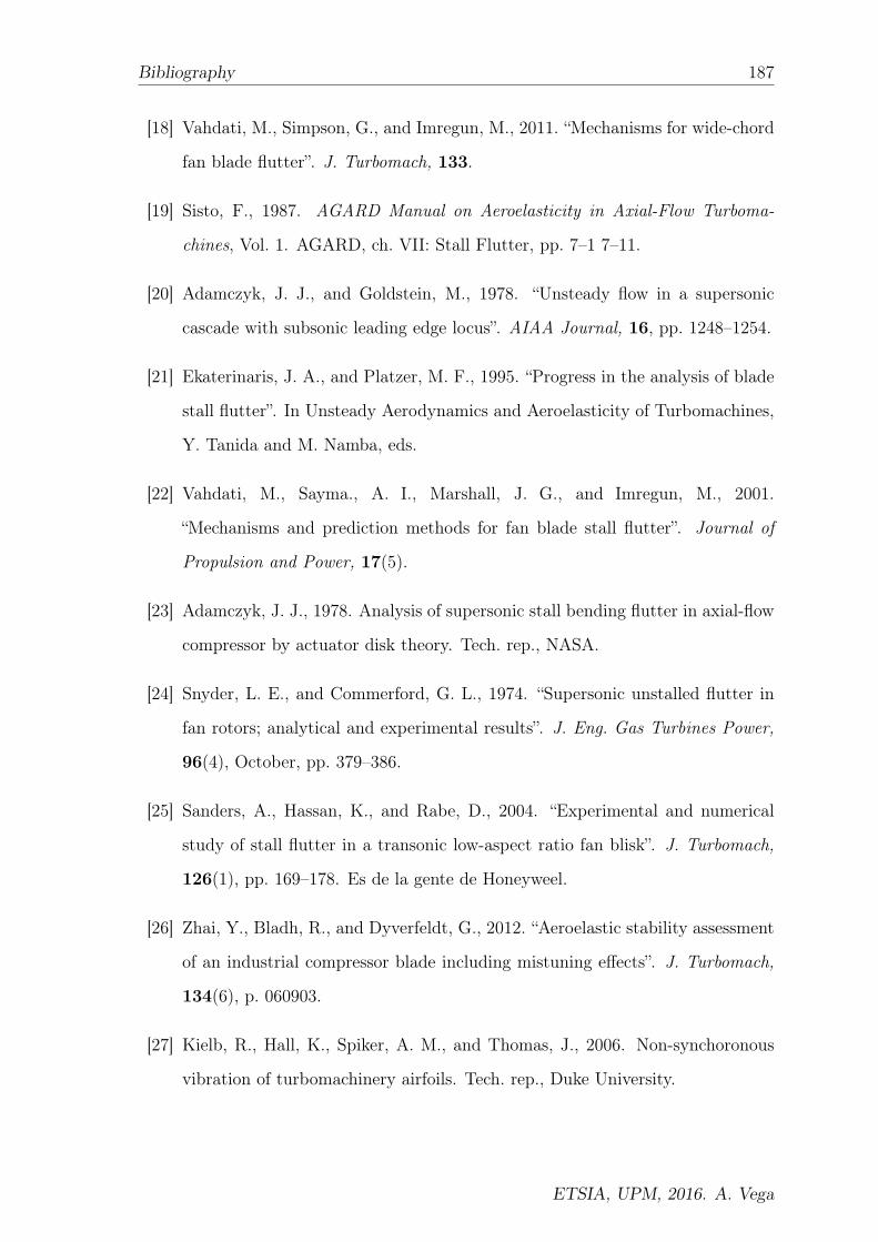
Bibliography 187
[18] Vahdati, M., Simpson, G., and Imregun, M., 2011. “Mechanisms for wide-chord
fan blade flutter”. J. Turbomach, 133.
[19] Sisto, F., 1987. AGARD Manual on Aeroelasticity in Axial-Flow Turboma-
chines, Vol. 1. AGARD, ch. VII: Stall Flutter, pp. 7–1 7–11.
[20] Adamczyk, J. J., and Goldstein, M., 1978. “Unsteady flow in a supersonic
cascade with subsonic leading edge locus”. AIAA Journal, 16, pp. 1248–1254.
[21] Ekaterinaris, J. A., and Platzer, M. F., 1995. “Progress in the analysis of blade
stall flutter”. In Unsteady Aerodynamics and Aeroelasticity of Turbomachines,
Y. Tanida and M. Namba, eds.
[22] Vahdati, M., Sayma., A. I., Marshall, J. G., and Imregun, M., 2001.
“Mechanisms and prediction methods for fan blade stall flutter”. Journal of
Propulsion and Power, 17(5).
[23] Adamczyk, J. J., 1978. Analysis of supersonic stall bending flutter in axial-flow
compressor by actuator disk theory. Tech. rep., NASA.
[24] Snyder, L. E., and Commerford, G. L., 1974. “Supersonic unstalled flutter in
fan rotors; analytical and experimental results”. J. Eng. Gas Turbines Power,
96(4), October, pp. 379–386.
[25] Sanders, A., Hassan, K., and Rabe, D., 2004. “Experimental and numerical
study of stall flutter in a transonic low-aspect ratio fan blisk”. J. Turbomach,
126(1), pp. 169–178. Es de la gente de Honeyweel.
[26] Zhai, Y., Bladh, R., and Dyverfeldt, G., 2012. “Aeroelastic stability assessment
of an industrial compressor blade including mistuning effects”. J. Turbomach,
134(6), p. 060903.
[27] Kielb, R., Hall, K., Spiker, A. M., and Thomas, J., 2006. Non-synchoronous
vibration of turbomachinery airfoils. Tech. rep., Duke University.
ETSIA, UPM, 2016. A. Vega

188 Bibliography
[28] Clark, S. T., Besem, F. M., Kielb, R., and Thomas, J. P., 2015. “Developing
a reduced-order model of nonsynchronous vibration in turbomachinery using
proper orthogonal decomposition methods”. Jounal of Engineering for Gas
Turbines and Power, 137(5), pp. 052501–11.
[29] Crawley, E., 1984. “Aeroelastic formulations for turbomachines and propellers”.
In Proceedings of the third International Symposium on Unsteady Aerodynam-
ics of Turbomachines and Propellers.
[30] Martel, C., Corral, R., and Llorens, J. M., 2008. “Stability increase of
aerodynamically unstable rotors using intentional mistuning”. J. Turbomach,
133, January, pp. 1–11.
[31] Kielb, J. J., and Abhari, R. S., 2003. “Experimental study of aerodynamic
and structural damping in a full-scale rotating turbine”. J. Eng. Gas Turbines
Power, 125(1), December, pp. 102–112.
[32] Corral, R., Escribano, A., Gisbert, F., Serrano, A., and Vasco, C., 2003.
“Validation of a linear multigrid accelerated unstructured navier-stokes solver
for the computation of turbine blades on hybrid grids”. In AIAA Paper 2003-
3326, 9th AIAA/CEAS Aeroacoustics Conference.
[33] Vogt, D., 2005. “Experimental investigation of three-dimensional mechanisms in
low-pressure turbine flutter”. PhD thesis, KTH Royal Institute of Technology.
[34] Szechenyi, E., Cafarelli, I., Notin, C., and Girault, J. P., 1984. “A straight
cascade wind-tunnel study of fan blade flutter in started supersonic flow”. In
Proceedings of the Third International Symposium on Unsteady Aerodynamics
of Turbomachines and Propellers, Cambridge, pp. 447–458.
[35] Crawley, E., and Hall, K. C., 1985. “Optimization and mechanisms of mistuning
in cascades”. J. Eng. Gas Turbines Power, 2, pp. 418–426.
ETSIA, UPM, 2016. A. Vega
Bibliography 189
[36] He, L., 1995. “Rotating-stall/stall-flutter prediction using a fluid/structure cou-
pled method”. In Unsteady Aerodynamics and Aeroelasticity of Turbomachines,
pp. 597–607.
[37] Vahdati, M., and Imregun, M., 1995. “Nonlinear aeroelasticity analysis using
unstructured dynamics meshes”. In Unsteady Aerodynamics and Aeroelasticity
of Turbomachines.
[38] Sayma, A. I., Vahdati, M., Green, J. S., and Imregun, M., 1998. “Whole-
assembly flutter analysis of a low pressure turbine blade”. In 8th International
Symposium in Unsteady Aerodynamics and Aeroelasticity of Turbomachines,
T. Fransson, ed., pp. 347–359.
[39] Gottfried, D. A., and Fleeter, S., 1999. “Aerodynamic damping predictions for
turbomachine blade rows using a three-dimensional time marching simulation”.
In AIAA/ASME/SAE/ASEE Joint Propulsion Conference and Exhibit.
[40] Sadeghi, M., and Liu, F., 2005. “Computation of cascade flutter by
uncoupled and coupled methods”. International Journal of Computational Fluid
Dynamics, pp. 559–569.
[41] Corral, R., and Gallardo, J., 2014. “Nonlinear dynamics of bladed disks with
multiple unstable modes”. AIAA Journal, 56(6), June, pp. 1124–1132.
[42] Verdon, J., and Caspar, J., 1984. “A linearized unsteady aerodynamic analysis
for transonic cascades”. Journal of Fluid Mechanics, 149, pp. 403–429.
[43] Giles, M. B., 1991. “A framework for multi-stage unsteady °ow calculations”.
In Proceeding of the Sixth International Symposium on Unsteady Aerodynam-
ics, Aeroacoustics and Aeroelasticity of Turbomachines and Propellers, H. M.
Atassi, ed.
[44] Chen, T., and He, L., 2001. “Analysis of unsteady blade row interaction using
nonlinear harmonic approach”. Journal of Propulsion and Power, 17(3), May-
June, pp. 651–658.
ETSIA, UPM, 2016. A. Vega

190 Bibliography
[45] Lane, F., 1956. “System mode shapes in the futter of compressor blade rows”.
Journal of the Aeronautical Sciences, 23(1), January, pp. 54–66.
[46] Wagner, H., 1925. Uber die Entstehung des dynamischen Auftriebes von
Tragflugeln. VDI-Verl.
[47] Garrick, I., 1937. Propulsion of a flapping and oscillating airfoil. Tech. Rep.
496, NACA.
[48] Mikolajczak, A. A., 1975. The practical importance of unsteady flow. Tech.
rep., AGARD CP-177.
[49] Platzer, M. F., 1977. Unsteady fflow in turbomachines - a review of current
developments. Tech. rep., AGARD CP-227.
[50] Sisto, F., 1978. A Moder Course in Aeroelasticity. E.H. Dowell.
[51] Whitehead, D. S., 1980. Unsteady aerodynamics in turbomachinery. in special
course on unsteady aerodynamics. Tech. rep., AGARD 679.
[52] Tijdeman, H., and Seebass, R., 1980. “Transonic flow past oscillating airfoils”.
Annual Review of Fluid Mechanics, 12, pp. 181–222.
[53] Verdon, J., 1987. Linearized unsteady aerodynamic theory. Manual on
aeroelasticity in axial-flow turbomachines, AGARD.
[54] Howe, M. S., 1998. Acoustics of Fluid-Structure Interactions. Cambridge
University Press.
[55] Saffman, P., 1992. Vortex Dynamics. Cambridge Monographs on Mechanics
and Applied Mathematics.
[56] Whitehead, D., 1970. Vibration and sound generation in a cascade of flat plates
in subsonic flow. Tech. rep., Aeronautical Research Council.
[57] Whitehead, D., 1987. Classical Two-Dimensional Methods, AGARD Manual
on Aeroelasticity in Axial-Flow Turbomachines. AGARD.
ETSIA, UPM, 2016. A. Vega

Bibliography 191
[58] Tyler, J. M., and Sofrin, T. G., 1961. “Axial flow compressor noise studies”.
SAE, 70.
[59] Lighthill, M., 1954. “The response of laminar skin friction and heat transfer to
fluctuations in the stream velocity”. Proceedings of the Royal Society of London,
224, pp. 1–23.
[60] Phillips, J., and Avkerberg, R. C., 1972. “A numerical method for integrating
the unsteady boundary-layer equations when there are regions of backflow”.
Journal of Fluid Mechanics, 58, pp. 561–579.
[61] McCroskey, W., and Philippe, J., 1975. “Unsteady viscous flow on oscillating
airfoils”. AIAA Journal, 13, pp. 71–79.
[62] Cebeci, T., 1977. “Calculation of unsteady two-dimensional laminar and
turbulent boundary layer with fluctuations in external velocity”. Proceedings of
the Royal Society of London, 355, pp. 225–238.
[63] Crawley, E., 1987. Manual on Aeroelasticity in Axial Flow Turbomachines-
Vol. 2, Structural Dynamics and Aeroelasticity. AGARD, ch. Aeroelastic
Formulation of Tuned and Mistuned Rotor, pp. 19–1 19–24.
[64] Hall, K., and Clark, W., 1993. “Linearized euler predictions of unsteady
aerodynamic loads in cascades”. AIAA Journal, 31, pp. 540–550.
[65] Lee, C., 1986. “An iterative procedure for non-linear flutter analysis”. AIAA
Journal, 24, pp. 833–840.
[66] Namba, M., 1972. Lifting surface theory for a rotating subsonic or transonic
blade row. Tech. rep., Aeronautical Research Council.
[67] F. Sisto, W. Wu, S. T., and Jonnavithula, S., 1989. “Computational
aerodyamics of oscillating cascades with the evolution of stall”. AIAA Journal,
27, pp. 462–471.
ETSIA, UPM, 2016. A. Vega

192 Bibliography
[68] Erdos, J., Alzner, E., and McNally, W., 1977. “Numerical solution of periodic
transonic flow through a fan stage”. AIAA Journal, 15(11), pp. 1559–1568.
[69] Giles, M., 1990. “Stator/rotor interaction in a transonic turbine”. Propulsion
and Power, 6, pp. 621–627.
[70] He, L., and Denton, J., 1993. “Inviscid-viscous coupled solution for
unsteady flows through vibrating blades. part i: Description of the method”.
Turbomachinery, 115, pp. 94–100.
[71] Lindquist, D., and Giles, M. B., 1991. “On the validity of linearized unsteady
euler equations with shock capturing”. In Proceedings of the AIAA.
[72] Montgomery, M., and Verdon, J., 1997. “A 3d linearized euler analysis
for bladerows. part i: Aerodynamic and numerical formulations”. In
Proceedings of the 8th International Symposium on Unsteady Aerodynamics
and Aeroelasticity of Turbomachines, pp. 427–444.
[73] Ning, W., and He, L., 1998. “Computation of unsteady flows around oscillating
blades using linear and non-linear harmonic euler methods”. ASME J.
Turbomach, 120, pp. 714–722.
[74] Clark, W. S., and Hall, K., 2000. “Atime linearized navier-stokes analysis of
stall flutter”. ASME J. Turbomach, 122, pp. 467–476.
[75] Sbardella, L., and Imregun, M., 2001. “Linearized unsteady viscous
turbomachinery flows using hybrid grids”. J. Turbomach, 123, pp. 568–582.
[76] K.C. Hall, J. T., and Clark, W., 2002. “Computation of unsteady non-linear
flows in cascades using a harmonic balance technique”. AIAA Journal, 40,
pp. 879–886.
[77] J. Crespo, R. C., and J.Pueblas, 2015. “An implicit harmonic balance method
in graphics processing units for oscillating blades”. ASME J. Turbomach, 138,
p. 031001.
ETSIA, UPM, 2016. A. Vega

Bibliography 193
[78] Corral, R., and Gallardo, J., 2011. “Non-linear dynamics of multi-mode unstable
bladed-disks: Part i - description of a canonical model and phenomenological
results”. In ASME Paper 2011-GT-22943.
[79] Crespo, J., Corral, R., and Pueblas, J., 2016. “An implicit harmonic balance
method in graphics processing units for oscillating blades”. J. Turbomach,
138(3), p. 031001.
[80] Vega, A., Corral., R., Zanker, A., and Ott, P., 2014. “Experimental and
numerical assessment of the aeroelastic stability of blade pair packages”. In
ASME Paper GT2014-25607, Proceedings of the 59st ASME Gas Turbine and
Aero engine Congress, Exposition and Users Symposium.
[81] Lindquist, D. R., and Giles, M. B., 1994. “Validity of linearized unsteady euler
equations with shock capturing”. AIAA Journal, 32(1), pp. 46–53.
[82] Corral, R., and Gisbert, F., 2003. “A numerical investigation on the influence
of lateral boundaries in linear vibrating cascades”. J. Turbomach, 125, July,
pp. 433–441.
[83] Burgos, M., Corral, R., and Contreras, J., 2011. “Efficient edge based
rotor/stator interaction method”. AIAA Journal, 41(1), January, pp. 19–31.
[84] Jameson, A., Schmidt, W., and Turkel, E., 1981. “Numerical solution of the
euler equations by finite volume techniques using runge-kutta time stepping
schemes”. In AIAA Paper 81-1259.
[85] Roe, P., 1981. “Approximate riemman solvers, parameters, vectors and
difference schemes”. Journal of Computational Physics, 43, pp. 357–372.
[86] Swanson, R. C., and Turkel, E., 1992. “On central-difference and upwinding
schemes”. Journal of Computational Physics, 101, pp. 292–306.
[87] Corral, R., Burgos, M. A., and Garcia, A., 2000. “Influence of the artificial
dissipation model on the propagation of acoustic and entropy waves”. In ASME
ETSIA, UPM, 2016. A. Vega

194 Bibliography
Paper 2000-GT-563, Proceedings of the 45th ASME Gas Turbine and Aero
engine Congress, Exposition and Users Symposium.
[88] Giles, M. B., 1990. “Non-reflecting boundary conditions for euler equation
calculations”. AIAA Journal, 28(12), pp. 2050–2057.
[89] Kirshner, A., Pelet, C., and Gyamarthy, G., 1976. “Investigation of bblade
flutter in a subsonic turbine”. Revue Francaise de Mécanique, numéro spécial,
pp. 97–104.
[90] Panovsky, J., and Kielb, R., 2000. “A design method to prevent low pressure
turbine blade flutter”. Journal of Engineering for Gas Turbines and Power,
122, pp. 89–98.
[91] Waite, J., and Kielb, R., 2015. “Physical understanding and sensitivities of low
pressure turbine flutter”. Journal of Engineering for Gas Turbines and Power,
137(1), p. 012502.
[92] Waite, J. J., and Kielb, R. E., 2015. “The impact of blade loading and unsteady
pressure bifurcations on low-pressure turbine flutter boundaries”. J. Turbomach,
138(4), December, pp. 041002–041002–9.
[93] Corral, R., and Vega, A., 2016. “The low reduced frequency limit of vibrating
airfoils - part i: Theoretical analysis”. J. Turbomach, 138(2), February,
p. 021004.
[94] Vega, A., and Corral, R., 2016. “The low reduced frequency limit of vibrating
airfoils - part ii: Numerical experiments”. J. Turbomach, 128(2), February,
p. 021005.
[95] Corral, R., and Vega, A., 2016. “Physics of vibrating turbine airfoils at low
reduced frequency”. AIAA Journal of Propulsion and Power, 32(2), March,
pp. 325–336.
ETSIA, UPM, 2016. A. Vega

Bibliography 195
[96] Barbarossa, F., Parry, A. B., Green, J. S., and di Mare, L., 2016. “An
aerodynamic parameter for low-pressure turbine flutter”. J. Turbomach, 138(5),
May, p. 051001.
[97] Lemmerman, L., and Sonnad, V., 1979. “Three-dimensional viscous-inviscid
coupling using surface transpiration”. Journal of Aircraft, 16(6), pp. 353–358.
[98] Wolff, J., and Fleeter, S., 1994. “Unsteady inviscid-viscous analysis of oscillating
aerodynamics”. In 30th Joint Propulsion Conference and Exhibit, Joint
Propulsion Conferences, AIAA, p. AIAA Paper 2797.
[99] Fransson, T. H., and Verdon, J. M., 1992. Updated report on standard
configurations for unsteady flow. Tech. rep., KTH.
[100] Vega, A., and Corral, R., 2013. “Physics of vibrating airfoils at low reduced
frequency”. In ASME paper GT2013-94906, Proceedings of the 58th ASME
Gas Turbine and Aero engine Congress, Exposition and Users Symposium.
[101] Corral, R., and Vega, A., 2016. “The low reduced frequency limit of vibrating
airfoils. part iiia: Theoretical quantification and influence of unsteady loading”.
In ASME Paper GT2016-57213, Proceedings of the 61th ASME Gas Turbine
and Aero engine Congress, Exposition and Users Symposium.
[102] Whitehead, D., and Evans, D., 1992. “Flutter of grouped turbine blades”. In
ASME Paper 92-GT-227.
[103] Kahl, G., 1995. “Application of the time linearized euler method to flutter
and forced response calculations”. In ASME Paper 95-GT-123, Proceedings of
the 40th ASME Gas Turbine and Aero engine Congress, Exposition and Users
Symposium.
[104] Chernysheva, O., Fransson, T., Kielb, R., and Barter, J., 2003. “Effect of sector
mode shape variation on the aerodynamic stability of a low-pressure turbine
sectored vane”. In ASME Paper 2003-GT-38632, Proceedings of the 48nd ASME
Gas Turbine and Aero engine Congress, Exposition and Users Symposium.
ETSIA, UPM, 2016. A. Vega

196 Bibliography
[105] Antona, R., Corral, R., and Gallardo, J., 2012. “Effect of the structural coupling
in the flutter onset of a sector of low-pressure turbine vanes”. J. Turbomach,
134, September, pp. 051007–1 051007–8.
[106] Zanker, A., Ott, P., and Calza, P., 2013. “Experimental aeroelastic
investigation of vibrating turbine blade cluster”. In 10th European Conference
on Turbomachinery, J. Bakman, G. Bois, and O. Leonard, eds., pp. 210–221.
[107] Bolcs, A., 1983. “Atestfaeffect for the investigation of steady and unsteady
transonic flows in annular cascades”. In ASME 83-GT-34.
ETSIA, UPM, 2016. A. Vega

Appendix A
Orthogonality of Aeroelastic Modes
Orthogonality of Travelling Wave Modes
The motion of a bladed-disc made up of N rotor blades vibrating as a traveling wave
of n nodal diameters (σn = 2πn/N ) and angular frequency ωn may be written as:
xnj = xn0 sin(ωnt+ jσn) (A.0.1)
where xnj , are the dispacements of the surface of the j-th airfoil. This motion
induces a force that, in first approximation, has as well the same travelling-wave
form: fnj = fn0 sin(ωnt + jσn + φ), where φ is the phase shift between the airfoil
motion and the force generated. In general, this force can contain higher spatial and
temporal harmonics but this fact does not change the argumentation. The work per
cycle exerted on the j-th rotor blade by the force fnj in another traveling-wave, with
another nodal diameter, m, and another frequency, ωm:
xmj = xm0 sin(ωmt+ jσm) (A.0.2)
can be expressed as:
wj =
ˆ T
0
fnj .xmj dt = fn0x
m0 ωm
ˆ T
0
sin(ωnt+ jσn + φ) cos(ωmt+ jσm) dt (A.0.3)
197
198 Appendix A. Orthogonality of Aeroelastic Modes
which after some operations leads to:
wj = 12fn0x
m0 ωm
ˆ T
0
sin
(ωn + ωm)t+ j 2π(n+m)N
+ φdt
+ 12fn0x
m0 ωm
ˆ T
0
sin
(ωn − ωm)t+ j 2π(n−m)N
+ φdt
(A.0.4)
If ωn 6= ωm the integral in time of the harmonic signal for each blade is null, since
Eq. A.0.5 represents the integration in time of a periodic signal. Only If ωn = ωm,
the second term of the integral gives rise to a non-null contribution:
wj = πfn0xm0 sin j(σn − σm) + φ . (A.0.5)
However, the work-per-cycle of the mode-shape is made up from the contributions of
all the rotor blades. Since Eq. A.0.5 represents a spatially harmonic signal, it can be
shown that
Wcycle =N∑i=1
wj = 0 (A.0.6)
It can be concluded that the traveling waves are orthogonal among them, and then,
the eigenfunctions of the aeroelastic problem are travelling waves. In particular the
work per cycle of a forward pressure TW with IBPA=σ in a backward TW with
IBPA=−σ is zero. Now, the question that arises is whether a standing wave can
also be solution of the aeroelastic problem (similarly to what happened in the purely
structural problem).
Non-orthogonality of Standing Wave Modes
The motion of a bladed-disc made up of N rotor blades vibrating as a standing-wave
of n nodal diameters (σn = 2πn/N ) and angular frequency ωn may be written as:
xnj = xn0 sin(ωnt) sin(jσn) (A.0.7)
where xnj , are the displacements of the surface of the j-th airfoil. This motion induces
a force that, in first approximation, has as well the same standing-wave form with a
phasing, both in space and time:
fnj = f0 sin(ωnt+ φ) sin(jσn + ϕ) (A.0.8)
ETSIA, UPM, 2016. A. Vega
199
The work per cycle on the j-th rotor blade of fnj in another standing-wave, with
another nodal diameter, m, and frequency, ωm:
xmj = xm0 sin(ωmt) sin(jσm + ψ) (A.0.9)
can be expressed as:
wj =
ˆ T
0
fnj .xmj dt = fn0x
m0 ωm
ˆ T
0
sin(ωnt+ φ) sin(jσn + ϕ) cos(ωmt) sin(jσm + ψ) dt
(A.0.10)
The phasing ψ, allows to take into account simultaneously the sine and cosine
components. Equation A.0.10 can in turn be written as:
wj = β
ˆ T
0
[cos((ωn − ωm)t)− cos((ωn + ωm)t)] cosφ dt
+ β
ˆ T
0
[sin((ωm − ωn)t) + sin((ωm + ωm)t)] sinφ dt
(A.0.11)
where β = 12fn0x
m0 ωm sin(jσn+ϕ) sin(jσm+ψ). If ωn 6= ωm then wj is obviously null,
however if ωn = ωm,wj = 2πβ cosφ/ωm. Exactly as in the TW case, the mode-shape
involves all the blades, and hence the total work,Wcycle =∑
j wj, has to be evaluated.
Wcycle = β′ˆ 2π
0
sin(nθ + ϕ− ψ) sin(mθ)dθ (A.0.12)
with β′ = π cosφfn0xm0 . The previous expression can be expanded as
Wcycle = β2
ˆ 2π
0
[cos(n−m)θ − cos(n+m)θ] cos(ϕ− ψ)dθ
+ β2
´ 2π
0[sin(n−m)θ + sin(n+m)θ] sin(ϕ− ψ)dθ
(A.0.13)
Obviously if n 6= m, Wcycle = 0. But, if n = m, it is Wcycle 6= 0for both, the
sine (ψ = 0) and cosine (ψ = π/2). This effectively means that the vibration of a
standing-wave of n nodal diameters, xnj = xn0 sin(ωnt) sin(jσn), produces work not
only in the sine component of the vibration but also in the cosine component xnj =
xn0 sin(ωnt) cos(jσn). This means that the standing waves are not eigenfunctions
of the aeroelastic problem. This is the ultimate reason of why a linear code for
aeroelastic computations is formulated in travelling wave terms.
ETSIA, UPM, 2016. A. Vega


