IMPACT OF SOCIO·ECONOMIC AND DEMOGRAPHIC FACTORS ON FOOD AWAY

FROM HOME CONSUMPTION IN THE UNITED STATES

Radolfo M. Nayga, Jr. • and

Qral Capps, Jr.

Abstract

This study identifies several socio-economic and demographic characteristics affecting food away from hor "onsumption using the recent 1987-88 National Food CODSumption Survey (the in"'· . _ mtake portion). The findings indicate that the following variables significantly affect the Immber of meals purchased: region, race, ethnicity, sex, household size, age, income, and time of week of consumption, The results also indicate that employed individuals consume more meals away from home than unemployed individuals.

Key words: food away from home, number of meals, type of faC1iii;j·, socio-economic and demographic factors,

-Lecturer, Department of Agricultural Economics and Business, Massey University, New Zealand and Professor, Department of Agricultural Economics, Texas A&M University, US~ respectively. .

1

Background

One of most noticeable changes in eating habits of consumers in recent years is the increased incidence of meals eaten outside the home. Very roughly, the change has been from about one meal in four to about one in three, an increase of about 33 percent during the last 25 years (Manchester, 1990). The percentage of disposable income going to food away from home (FAFH) has increased from 5.5 percent in 1970 to 6.2 percent in 1989 (Table 1). In contrast, the percentage of disposable income going to food at home (FAR) has declined monotonically from 10.8 percent in 1970 to 7.6 percent in 1989. These economic trends point to the increasing importance of FAFH consumption relative to FAH consumption.

The move toward eating out is prompted by changes in consumer lifestyles as well as changes in the socio-demographic structure of the u.s. population. Some socio-economic and demographic factors that come into play are: a growing number of women, married and single, in the work force: increasing importance of convenience in eating out; more families living on two incomes; the impact of advertising and promotion by large food service chains; and more people in the age group of 25 to 44 who are inclined to eat out often (Putnam and Van Dress, 1984). only about seven percent of all households now fit the old stereotype family of a working husband, a wife who does not work for wages, and two children (Kinsey, 1990). Moreover, married couples with children are declining as a share of all households. The one-adult households are fastest growing and are likely to exhibit 11on­conventional food consumption patterns (i.e. FAFH consumption).

The away from home market is composed of commercial foodservice establishments (i.e. restaurants, fast food places, cafeteria) and noncommercial outlets ( i. e. school or military dining rooms, child care centers). Although noncommercial outlets serve more food to more people, they account for only 30 percent of the total retail value of FAFH. A breakdown o.f nominal expendi tures for FAFH by type is given in Table 2. Eating and drinking places have the notable share of expenditures, 67 percent in 1989. Hotels and motels accounted for 5 percent of FAFH expenditures in 1989; schools and colleges almost 8 percent, and all other places nearly 13 percent.

Over the years, the place of consumption has changed within the FAFH market. In the past, full service restaurants accounted for the bulk of the FAFH sales. However, as McCracken and Brandt reported,. the number of fast food establishments has more than tripled in the last twenty five years. In terms of sales, the percentage change from 1972 to 1987 in restaurants was close to 300 percent compared to about. 500 percent in fast food facilities (U.S. Oepartment of Commerce). These structural changes wi thin the FAFH market will continue to have varying impacts on the various marketing programs and strategies of the different types of FAFH facility.

A number of studies on food away from home (FAFH) {see

below) have been made in recent years. Many of these studies have

focused their analyses on socio-demographic and economic factors

affecting the away from home food consumption and expenditure using

cross-sectional data from national samples. Common socio­

demographic factors consiiered were income, household size,

urbanization I region I race, employment, and education. Some of the

resul ts from these studies have differed regarding the relative

importance of these factors on FAFH consumption or expenditures,

primarily due to the use of different consumption models, data

bases, and estimation techniques. Prochaska and Schrimper (1973), using expenditures on meals

and the number of meals. purchased away from home as dependent

variables, found that the value of homemaker's time is an important

factor affecting food consumption, when the household is viewed as

both a producing and consuming unit. Their results showed a

posi ti ve effect of opportunity cost of time on away-from-home

consumption. Kinsey (1983) tested the effect of various sources of

household income on the marginal propensity to consume FAFH for

both white and nonwhi te households. Kinsey disaggrega.ted the

households by intensity of the wife's labor force participation and

by income and found that income earned by wives working full time

did not increase the marginal propensity to consume FAFH. Redman

(1980), on the other hand, examined the effects of women's time

allocation and socio-economic variables on the expenditures on

meals away from home and on prepared foods. .Results indicate that

employed wives buy more prepared foods but not more meals away from

home compared to unemployed wives. So far, only the works by McCracken and Brand (1987)

examined away from home consumption by type of facility

(restaurants, fast-food facili ties, and other commercial

facilities). Using the 1977-78 National Food Consumption Survey

(NFCS) data set and Tobit analysis, they identified and measured

the influence of factors affecting FAFH consumption by type of

facility. The factors included in the analyses are various socio­

economic factors as well as a variable depicting the value of the

household's time. They found that increases in income were

associated with increases in FAFM expenditure, but at a decreasing

rate. As well, the value of the household manager's time was

positively related to total FAFH expenditure, fast food, and other

commercial expenditures but was only marginally significant for

restaurant expenditures. Wi th the exception of the McCracken and Brandt piece, no

stUdies as yet have analyzed the effect of the individual's

employment status and other socio-demographic and economic factors

on FAFH consumption by type of faci Ii ty. Furthermore, J.fcCracken

and Brandt's study used the 1977-78 NFCS data set and, therefore,

their analysis may not reflect current market condi tions ~ The FAFH

industry I particularly the restaurant and fast food L \dustries I

would benef it from a study that would provide some it. formation

regarding the effect of various demographic and socio -economic

factors on FAFH consumption by type of facility. As well, the

comparison of the results of a study about FAFH consumption, using

3

the recent 1987-88 NFCS data set, with those of other studies on FAFH consumption (i.e. McCracken and Brandti Prochaska and Schrimper) using previous NF~S data sets could provide additional insights about the structur~l changes that have occurred in the FAFH industry in the past ~everal years.

This article attempts to fill this void by using the Individual Intake phase of the 1987-1988 National Food Consumption Survey. The objective of this study, therefore, is to determine factors affecting FAFH consumption by type of facility, using number of meals purchased as a measure of consumption.

conceptual Framework for ~e Analysis

Due to the unavailability of the household food use or expenditure phase of the 1987-88 NFCS data set during the completion stage o.f this study, number of meals is used in lieu of expendi tures as a measure of FAFH consumption. Pro.chaska and Schrimper also used the number of meals purchased away from home as a measure of FAFH consumption in their study. rl'he nUlnber of meals variable is a measure of the frequency that an individual ate FAFH.

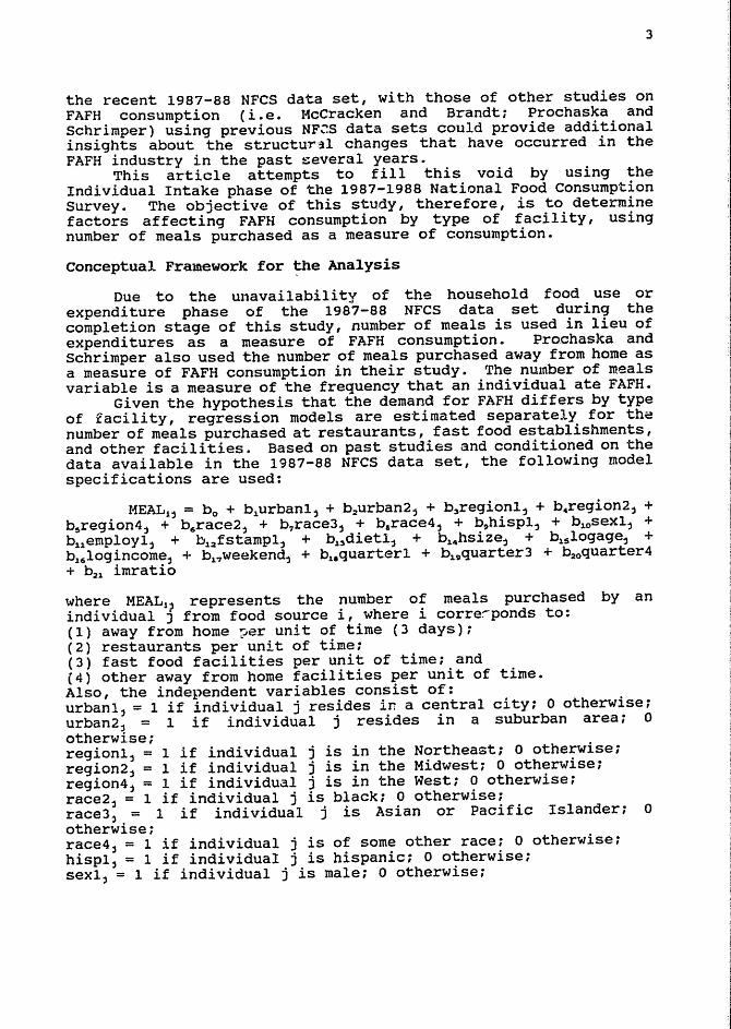
Given the hypothesis that the demand for FAFH differs by type of facility, regression models are estimated separately for the number of meals purchased at restaurants, fast food establishments, and other facilities. Based on past studies and conditioned on the data available in the 1987-88 NFCS data set, the following model specifications are used:

MEAL!j = bo + b1urbanl j + b 2urban2 j + b,regionl j + b.region2j + bsregion4 j + b6 race2 j . + b,race3 j ?" b.race4

b + ~9hisP1j + b1osex1j +

bllemploy1 j + b1.2 fstamp1 j + b13d~etlj + 14hs~zej + bl!'.logagej + b16logincomej + b1?weekendj + bu quarterl + bu quarter3 + b2oquarter4 + b2 1. imratio

where MEAL1~ represents the number of meals purchased by an individual J from food source i, where i corre~ponds to: (1) away from home ?er unit of time (3 days); (2) restaurants per unit of timei (3) fast food facilities per unit of time: and (4) other away from home facilities per unit of time. Also, the independent variables consist of: urbanl j = 1 if individual j resides in a central city: 0 otherwise; urban2 j = 1 if individual j resides in a suburban area; 0 otherwise: regionl j = 1 if individual j is in the Northeast; 0 otherwise; region2 j = 1 if individual j is in the Midwest; 0 otherwisei region4; = 1 if individual j is in the Westi 0 otherwise; race2 j = 1 if individual j is black: 0 otherwise: race3 j = 1 if individual j is Asian or Pacific Islanderi 0 otherwise; race4 j = 1 if individual j is of some other racei 0 otherwise; hisplj = 1 if individual j is hispanic: 0 otherwise; sexl j = 1 if individual j is malei 0 otherwise;

4

employlj = 1 if individual j is employed; 0 otherwise:

fstampL, = 1 if individual j is receiving food stamps; 0 otherwise;

dietl; = 1 if individual j is on a special diet; 0 otherwise;

hsize j = household size of individual j:

logagej = the logarithm of age of individual j;

logincome j = the logarithm of income of individual j:

weekend, = 1 if the three-day intake of individual j occurred

mostly during a weekend; 0 otherwise; and quarterl, quarter3, and quarter4 = correspond to a set of binary

variables that measure seasonality, (qaurterl=l if January -March;

quarter3=1 if July-september; quarter4=1 if october-December)

(reference category, Apri~-June).

One classification is eliminated from each group of variables

to avoid perfect collinearity among the exogenous variables and the

intercept (the so-called dummy varl able trap). The base group are

indi viduals who satisfy the following description: reside in a

nonmetro area (urban3 ); located in the South (region3 ) ; white

(racel); nonhispanic (hisp2) i female (sex2); unemployed (employ2);

not participating in the food stamp program (fstamp2); not on a

special diet (diet2); and the three-day intake occurred mostly

during a weekday (weekday). Household income is used instead of

individual income because the NFCS data set only provides income

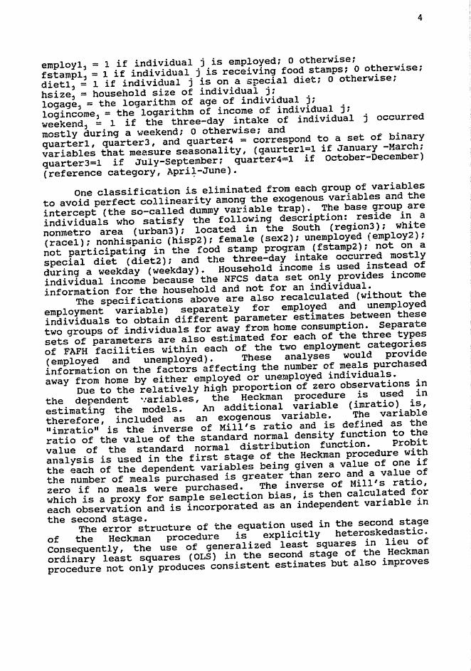
information for the household and not for an individual. The specifications above are also recalculated (without the

employment variable) separately for employed and unemployed

individuals to obtain different parameter estimates between these

two groups of individuals for away from home consumption. separate

sets of parameters are also estimated for each of the three types

of FAFH facilities within each of the two employment categories

(employed and unemployed). These analyses would provide

information on the factors affecting the number of meals purchased

away from home by either employed or unemployed individuals.

Due to the relatively high proportion of zero observations in

the dependent ':ariables, the Heckman procedure is used in

estimating the models. An addi tional variable ( imratio ) is,

therefore, included as an exogenous variable. The variable

"imratio" is the inverse of Mill's ratio and is defined as the

ratio of the value of the standard normal density function to the

value of the standard normal distribution function. Probit

analysis is used in the first stage of the Heckman procedure with

the each of the dependent variables being given a value of one if

the number of meals purchased is greater than zero and a value of

zero if no meals were purchased. The inverse of Mill's ratio,

which is a proxy for sample selection bias, is then calculated for

each observation and is incorporated as an independent variable in

the second stage. The error structure of the equation used in the second stage

of the Heckman procedure is explicitly heteroskedastic.

Consequently, the use of generalized least squares in lieu of

ordinary least squares (OLS) in the second stage of the Heckman

procedure not only produces consistent estimates but also improves

5

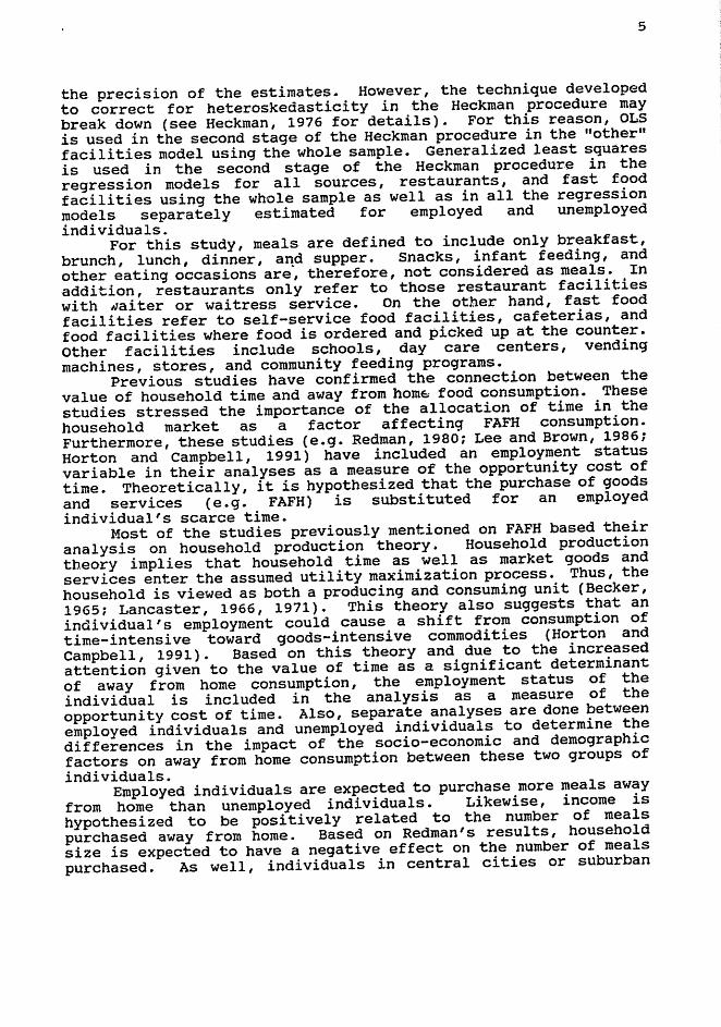
the precision of the estimates. However, the technique developed to correct for heteroskedasticity in the Heckman procedure may break down (see Heckman, 1976 for details). For this reason, OLS is used in the second stage of the Heckman procedure in the "othern faci Ii ties model using the whole sample. Generalized least squares is used in the second stage of the Heckman procedure in the regression models for all sources, restaurants, and fast food facilities using the whole sample as well as in all the regression models separately estimated for employed and unemployed individuals.

For this study, meals are defined to include only breakfast, brunch, lunch, dinner, aI1d supper. Snacks, infant feeding, and other eating occasions are, therefore, not considered as meals. In addition, restaurants only refer to those restaurant facilities withIJaiter or waitress service. On the other hand, fast food facilities refer to self-service food facilities, cafeterias, and food facilities where food is ordered and picked up at the counter. Other facilities include schools, day care centers, vending machines, stores, and community feeding programs.

Previous studies have confirmed the connection between the value of household time and away from hom6 food consumption. These studies stressed the importance of the allocation of time in the household market as a factor affecting FAFH consumption. Furthermore, these studies (e.g. Redman, 1980; Lee and Brown, 1986; Horton and Campbell, 1991) have included an employment status variable in their analyses as a measure of the opportunity cost of time. Theoretically, it is hypothesized that the purchase of goods and services (e.g. FAFH) is substituted for an employed individual's scarce time.

Most of the studies previously mentioned on FAFH based their analysis on household production theory • Household production theory implies that household time as well as market goods and services enter the assumed utility maximization process. Thus, the household is viewed as both a producing and consuming unit (Becker, 1965; Lancaster, 1966, 1971). This theory also suggests that an individual's employment could cause a shift f.rom consumption of time-intensive toward goods-intensive commodities (Horton and Campbell, 1991). Based on this theory and due to the increased attention given to the value of time as a significant determinant of away from home consumption, the employment status of the individual is included in the analysis as a measure of the opportunity cost of time. Also, separate analyses are done between employed individuals and unemployed individuals to determine the differences in the impact of the socio-economic and demographic factors on away from horne consumption between these two groups of individuals.

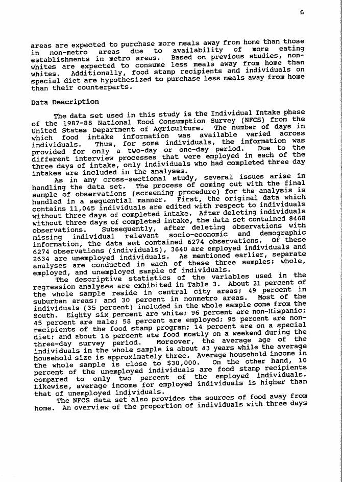
Employed individuals are expected to purchase more meals away from home than unemployed individuals. Likewise, income is hypothesized to be positively related to the number of meals purchased away from home. Based on Redman's results, household size is expected to have a negative effect on the number of meals purchased. As well, individuals in central cities or suburban

G

areas are expected to purchase more meals away from home than those

in non-metro areas due to availability of more eating

establishments in metro areas. Based on previous studies I non­

whites are expected to consume less meals away from home than

whi tes. Addi tionally, food stamp recipients and individuals on

special diet are hypothesized to purchase less meals away from home

than their counterparts.

Data Description

The data set used in this study is the Individual Intake phase

of the 1987-88 National Rood Consumption Survey (NFCS) from the

United states Department of Agriculture. The number o.f days in

which food intake information was available varied across

indi viduals. Thus I for some individuals, the information was

provided for only a two-day or one-day period. Due to the

different interview processes that were employed in each of the

three days of intake, only individuals who bad completed three day

intakes are included in the analyses .. As in any cross-sectional study, several issues arise in

handling the data set. The process of coming out with the final

sample o.f observations (screening procedure) for the analysis is

handled in a sequential manner. First, the original data which

contains 11,045 individuals are edited with respect to individuals

wi thout three days of completed intake. After deleting individuals

without three days of completed intake, the data set contained 8468

observations. Subsequently, after deleting observations with

missing indi vidual t"elevant socio-economic and demographic

information, the data s~t contained 6274 observations. Of these

6274 observations (individuals), 3640 are employed individuals and

2634 are unemployed individuals. As mentioned earlier, separate

analyses are conducted in each of these three samples: whole,

employed, and unemployed sample of individuals. 'rhe descriptive statistics of the variables used in the

regression analyses are exhibited in Table 3. About 21 percent of

the whole sample reside in central city areas; 49 percent in

suburban areas; and 30 percent in nonmetro areas. Most of the

indi viduals (35 percent) included in the whole sample come from the

South. Eighty six percent are white; 96 percent are non-Hispanic;

45 percent are maleiS8 percent are employed; 95 percent are non­

recipients of the food stamp program; 14 percent are on a special

diet; and about 16 percent ate food mostly on a weekend during the

three-day survey period. Moreover, the average age of the

indi viduals in the whole sample is about 43 years while the average

household size is approximately three. Average household income in

the whole sample is close to $30 I 000. On the other hand I 10

percent of the unemployed individuals are food stamp recipients

compared to only two percent of the employed individuals.

Likewise, average income for employed individuals is higher than

that of unemployed individuals. The NFCS data set 'also provides the sources of food away from

home. An overview of the proportion of individuals with three days

7

of completed intake eating food away from home by source of food is given in Table 4. About 48 percent of the individuals had not consumed any FAFH meal during the three day survey period. In addi tion, larger portions of the individuals have not consumed food in either restaurants, fast food facilities, or other facilities. For example, less than 30 percent of the sample consumed food from either restaurants, fast food facilities, or other facilities ..

The descriptive statistics of the dependent variables used are shown in Table 5. For the whole sample, the maximum number o.f meals purchased by an individual is ninp. from either all sources or restaurants. The maximum number of meals purchased from fast food facilities or other facilities by an individual is eight. The av.erage number of meals purchased, on the other hand, from all sources is 1.05. By type of facility, the average number of meals purchased from restaurants, fast food facili ties, and other facilities is 0.38, 0.50, and 0.17, respectively. As expected, the average number of meals purchased by employed individuals in every type of facility is higher than that of the uflemployed individuals.

Empirical Results

In this section, the Heckman procedure results are reported separately for the number of meals purchased away from home and for the number of meals purchased from restaurants, fast food facilities, and other away from home facilities. The results on the separate regression analyses on employed and unemployed individuals are presented subsequently.

Number of l.feals Consumed Away fr:om Home

The Heckman procedure results (using the whole sample) for number of meals purchased away from home and by type of eating facility are exhibited in Table 6.. The Heckman procedure estimates for the number of meals purchased away from home indicate that the regional variables as a group are statistically significant as indicated by the joint F test. In particular, individuals from the Midwest and the west generally purchase fewer meals away from home than individuals from the South. Redman's study revealed that households in the North Central region generally have lower expenditures from FAFH compared to households in the west. The race dummy variables as a group are also statistically significant. Interestingly t individuals of "othern races purchase more meals away from home than whites. In contrast to the results from the Prochaska and Schrimper study, non-whi tes ( i • e . blacks I Asians, Pacific Islanders) do not consume fewer meals away from home than whites. Hispanics, however, consume fewer meals away from home than non-Hispanics.

Males purchase more meals away from home than females. In contrast to the resul t in Redman's study on women, employed indi vidualspurchase more meals away from home than unemployed individuals. This result supports the hypothesis that individuals wi th higher opportunity cost of time ( i . e. employed individuals

8

vis-a-vis unemployed individuals) purchase and consume more meals away from home. Not surprisingly, individuals on special diet consume fewer meals away from home than those who .are not on special diet.

Household size is negatively related to the number of meals purchased away from home. This result is consistent with the findi.ng in the McCracken and Brandt study which used FAFH expenditures. Interestingly, individuals who consumed FAFH during the weekend purchased fewer meals away from home than those indi viduals who consumed FAFH during the weekday. As expected, age (income) is negatively (positively) related to the number of meals purchased away from home •.

Number of Meals Consumed Away from Home by Tvpe of Facility

The Heckman procedure estimates (using the \<lhole sample) for the number of meals consumed from restaurants, fast food facilities, and other away from home food facilities in Table 6 reveal differences as per significance of the various socio­demographic factors by type of FAFH establishment.

The number of meals consumed from either restaurants, fast food facilities, or other facilities are significantly affected by regional factors. McCracken and Brandt did not find any significant regional effects on expenditures on any FAFH facility. In particular, the regression estimates indicate that individuals from the Northeast consume more meals from restaurants compared to individuals from the South. In addition, individuals from the Midwest and West purchase fewer meals from fast food facilities than individuals from the South. Individuals from the West, however, consume fewer meals from other facilities than individuals from the South. In terms of race, individuals of nother" races consume more meals from other facilities than whites. Males consume more meals from either restaurants or fast food facilities than females.

In accord with prior expectations and with McCracken and Brandt's study on FAFH expenditures, employed individuals consume more meals from fast food facilities but not from restaurants than unemployed indi \riduals. As well, employed individuals do not consume more meals from other away from home food facilities than unemployed individuals. In addition, income is not statistically significant in any of the three FAFH facilities. These findings may suggest that individuals eat at restaurants not only to save time but also to acquire some recreational di version. These results also suggest that eating away from home in restaurants and fast food facilities depends less on income than on the value of the indi vidual's time assuming that employed indi viduals have higher opportunity costs of time than unemployed individuals.

Indi viduals who consumed FAFH during the weekend purchase fewer meals from either restaurants, fast food facilities, or other facilities than those who consumed FAFH during the weekday. Household size, as expe'cted, is negatively related to the number of meals purchased from restaurants and fast food facilities. This

I

9

finding on nousehold size indicates a decreasing affinity of eating at either restaurants or fast food facilities with increasing household size. Age is also negatively related to the number of meals purchased from fast food facilities and other facilities. Seasonality, however, is not a statistically significant factor affecting number of meals purchased in any of the three types of facility.

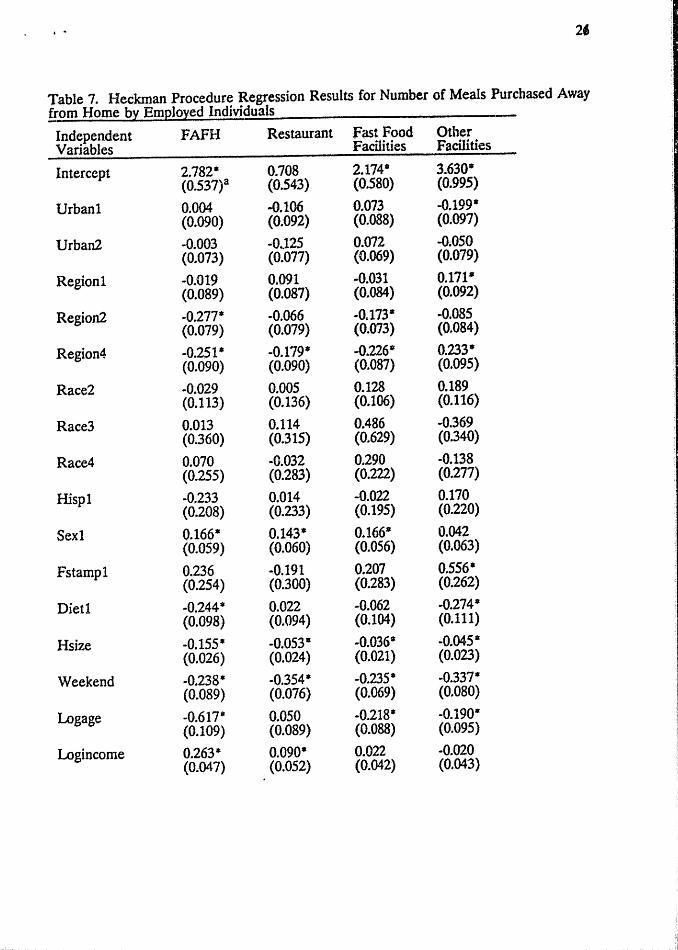
Analyses on Employed and Unemployed Individuals

separate sets of parameters are estimated for employed and unemployed individuals to.determine the various factors affecting FAFH consumption by type of facility between these two sets of individuals. The Heckman procedure is employed in all the regression runs I using generalized least squares in the second stage of the estimation process. The parameter estimates, along with their standard errors are presented in Tables 7 and 8. As expected, the adjusted R-squared of the models are relatively low al though reasonable considering the cross-sectional (sample of indi viduals) nature of the dat.a used.

Joint F-tests are conducted for each of the group of urbanization, regional, race, and Seasonal variables. These tests indicate that regional variables as a group are statistically significant in all of the four regression models estimated for employed individuals but not for unemployed individuals. The race variables as a group are statistically significant in two (all sources and other faci Ii ties )of the four regression models for unemployed individuals.

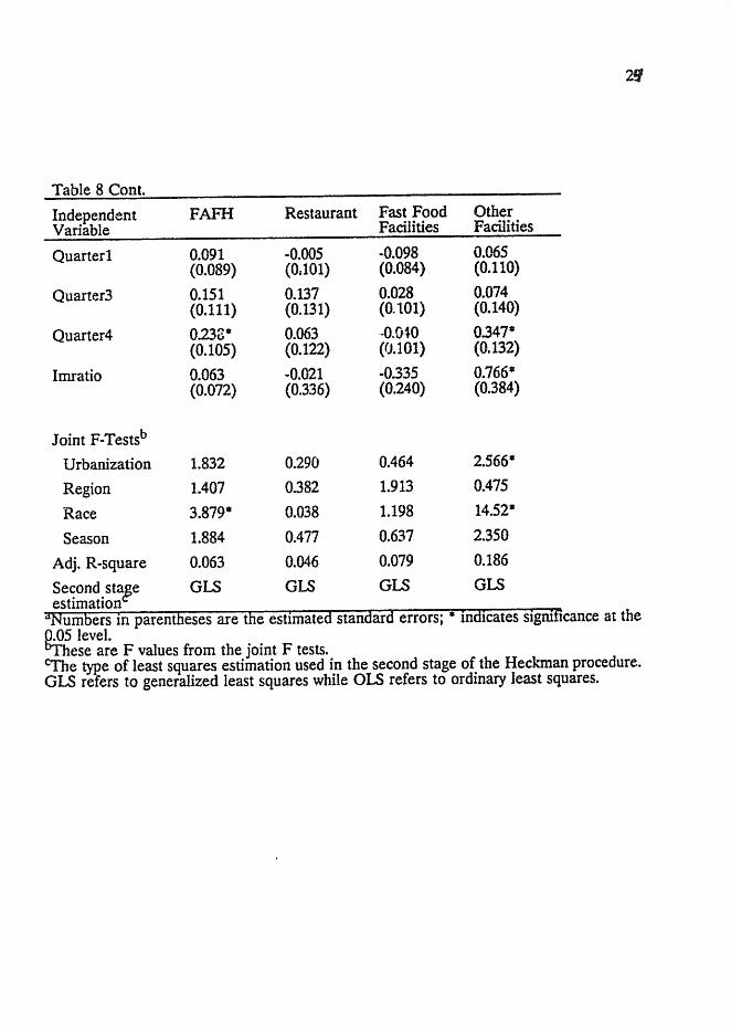
As shown in Table 7, the significant factors affecting the number of meals purchased away from home from all sources by employed individuals include region, sex, special diet, household size, time of the week of consumption, age, and income. By the s.ame token, the statistically significant factors in the models for unemployed individuals are only race, sex, and age (see Table 8). Hence, the impact of the variables depicting special diet, household size, and time of week of consumption on the number of meals purchased away from home are not as important for unemployed individuals as opposed to employed individuals.

As well, more socio-economic and demographic factors significantly affect the number of meals purchased in restaurants, fast food facilities, and other facilities by employed individuals than unemployed individuals. Among employed and unemployed individuals for instance, males purchase more meals than females in restaurants and fast food facilities. For employed individuals, those in larger households and those who consumed their food mostly on a weekend purchase significantly less meals in restaurants and fast food facilities than their counterparts. This result contrasts to that among unemployed individuals where the effect of household size and time of week of consumption on the number of meals purchased in restaurants and fast food facilities are not statistically significa·nt. Moreover, the number of meals purchased in restaurants significantly increases with income among employed

10

individuals but not among unemployed individuals. Among employed indi viduals I the impact of the fo':"lowing factors: food stamp participation I special diet I hOllseh(}ld size, time of week of consumption, age, and region on the llumber of meals purchased in "other" away from home facilities arl-::' statistically significant. Race, time of week of consumption, and age are the only statistically significant factors affecting the number of meals purchased by unemployed individuals in "other" facilities.

Concluding Comments

Increased attention has been devoted in recent years to the analysis of FAFH consumptl.on patterns mainly due to the growing appeti te by Americans for eating out. This study not only determines the factors affecting total FAFH consumption but also examines, at a disaggregate level, the consumption patterns of the types of facilities wi thin the FAFH industry. The FAFH consumption measure used is number of meals purchased by an individual.

The findings from the model for all types of FAFH facilities indicate that the following variables significantly affect the number of meals purchased: region, race, ethnicity, sex, household size, age, income, and time of week of consumption. Importantly, the results also indicate that employed individuals consume more meals away from home than unemployed individuals. This result supports the hypothesis that individuals with higher opportunity cost of time, assuming that employed individuals have higher opportunity cost of time than unemployed individuals, purchase and consume more meals away from home. Among employed individuals I the significant factors affecting the number of meals purchased away from home are region, sex, special diet, household size, time of week of consumption I age I and income. In contrast, only race, sex, and age are the factors significantly affecting the number of meals purchased away from home by unemployed individuals.

The disaggregate regression estimates for the number of meals consumed from restaurants, fast food facilities, and other away from home food facilities reveal differences in significance of the various socio-demographic factors by type of FAFH establishment. In accord with prior expectations, the resul ts indicate that employed individuals consume more meals from fast food facilities and restaurants than unemployed indi viduals. Income is not statistically significant in any of the three models on FAFH facilities. These findings may suggest that individuals eat at restaurants not only to save time but also to acquire some recreational diversion. lwforeover, these results may suggest that consuming meals away from home in restaurants and fast food facilities depends less on income than on the employment status of the individual.

These results may be of considerable importance for the restaurant, fast food, and other away from home industries. For instance, the findings in this study suggest that marketing efforts by these FAFH industries should be focused on individuals who purchase relatively fewer meals away from home. These individuals

11

may include those with larger household sizes, females, those who are unemployed, and even those who are on special diets. The fa~t food industry (includes cafeterias arld self-service restaurants this study) also may wish to cater to the tastes of older people i.

efforts to boost sales.

12

References

Becker, G.S. (1965). A Theory of the Allocation of Time. Economic Journal, 75, 493-517.

Food Retailing Review, 1991 Edition, The Food Institute, January 1991.

Heckman, J.J. (1976). The Common structure of statistical Models of Truncation, Sample Selection and Limited Dependent Variables and a simple Estimator for Such Models. Annals of Economic a Social Measurement, 5, 475-492.

Horton, S. & Campbell, c. (1991). Wife's Employment, Food Expendi tures , and Apparent Nutrient Intake: Evidence from Canada. American .Journal of Agricultural Economics, 73, 784-94.

Kinsey, J. (1983). Working Wives and the Marginal Propensity to Consume Food Away From Home. American Journal of Agricultural Economics, 65, 10-19.

Kinsey, J. (1990). Diverse Demographics Drive the Food Industry,1i Choices, 2nd Quarter, p. 23.

Lancaster, K. (1966). A New Approach to Consumer Theory. Journal of Political Economy, 74, 132-57.

(1971). Consumer Demand. New York: ~olumbia University Press.

Lee, J. & Brown. M. (1986). Food Expenditures at Home and Away from Home in the United States- A Switching Regression Analysis~ The Review of Economics and statistics, 68, 142-47.

Maddala, G. s. (1983). Limited pependent and Oualitative Variables in Econometrics. cc:u.:""ridge Uni versi ty Press. Manchester, A.C. (1990). Food Expenditures at a Glance.

National Food Review, ERS-USDA, 13, 25. McCracken, V.A. & Brandt, J.A. (1987). Household Consumption of

Food Away From Home: Total Expenditure and by Type of Food Facility. American Journal of Agricultural Economics, 69, 274-284.

Pindyck, R.S. & Rubinfeld, D.L. (1991). Econometric Models and Economic Forecasts, Third Edition. McGraw-Hill.

Prochaska, F.J. & Schrimper, R.A. (1973). Opportunity Cost of Time and Other Socioeconomic Effects on Away from Home Food Consumption. American Journal of Agricultural Economics, 55, 595-603.

Putnam, J.J. & Van Dress, M.G. (1984). Changes Ahead for Eating Out. National Food Review, 26, 15-17.

Redman, B. (1980). The Impact of Women's Time Allocation on Expendi ture for Meals Away from Home and Prepared Foods. American Journal of Agricultural Economics, 62, 234-37.

U.S. Dept. of Agriculture, National Food Situation, Economic Research Service, Washington D.C., various issues.

U.s. Dept. of Commerce, Bureau of Census, 1987 Census of Retail Trade, Washington, D.C.

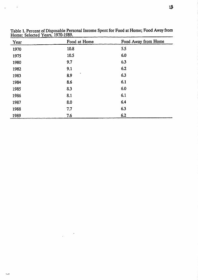
Table 1. Percent of Disposable Personal Incolne Spent for Food at Home; Food Away from Home: Selected Years, 1970-1989.

Year Food at Home Food Away from Home

1970 10.8 55 1975 10.5 6.0 1980 9.7 6.3 1982 9.1 6.2 1983 8.9 6.3 1984 8.6 6.1 1985 8.3 6.0 1986 8.1 6.1 1987 8.0 6.4

1988 7.7 6.3 1989 7.6 6.2

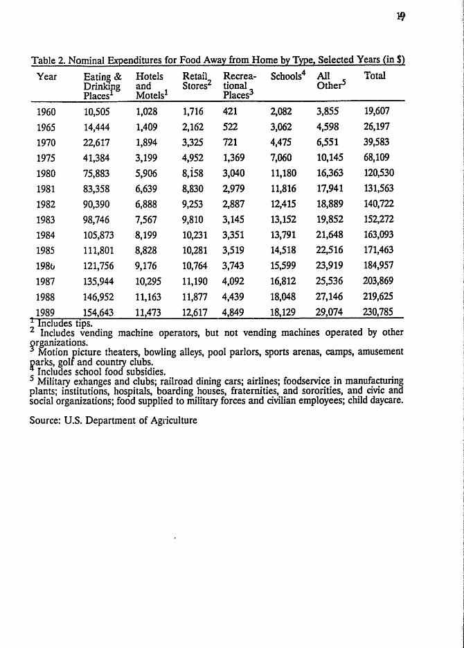
Table 2. Nominal Expenditures for Food Away" from Home by" Typez Selected Years {in Sl Year Eatin~ & Hotels Retail Recrea- Schools4 All Total

Drinkipg and Stores2 tional Othe~ Places Motels! Places3

1960 10,505 1,028 1,716 421 2,082 3,855 19,607

1965 14,444 1,409 2,162 522 3,062 4,598 26,197

1970 22,617 1,894 3,325 721 4,475 6,551 39,583

1975 41,384 3,199 4,952 1,369 7,060 10,145 68,109

1980 75,883 5,906 8,i58 3,040 11,180 16,363 120,530

1981 83,358 6,639 8,830 2,979 11,816 17,941 131,563

1982 90,390 6,888 9,253 2,887 12,415 18,889 140,722

1983 98,746 7,567 9,810 3,145 13,152 19,852 152,272

1984 105,873 8,199 10,231 3,351 13,791 21,648 163,093

1985 111,801 8,828 10,281 3,519 14,518 22,516 171,463

1986 121,756 9,176 10,764 3,743 15,599 23,919 184,957

1987 135,944 10,295 11,190 4;092 16,812 25,536 203,869

1988 146,952 11,163 11,877 4,439 18,048 27,146 219,625

1989 154,643 11,473 12,617 4,849 18,129 29,074 230,785 1 Includes tips. 2 Includes vending machine operators, but not vending machines operated by other ~rganizations.

Motion ficture theaters, bowling alleys, pool parlors, sports arenas, camps, amusement ~arks, gol and country clubs.

Includes school food subsidies. 5 Military exbanges and clubs; railroad dining cars; airlines; foodservice in manufacturing plants; institutions, hospitals, boarding houses, fraternities, and sororities, and civic ami social organizations; food supplied to military forces and civilian employees; child daycare.

Source: U.S. Department of Agriculture

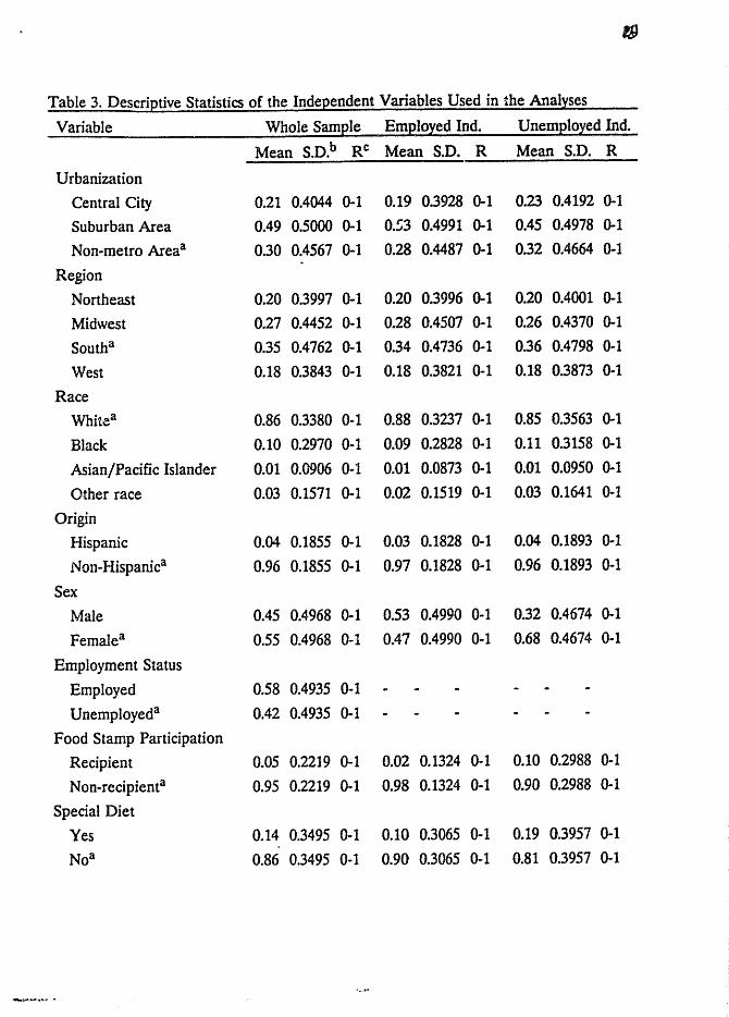
Table 3. Descriptive Statistics of the Independent Variables Used in the Analyses

Variable Whole Sample Employed Ind. Unemployed Ind.

Urbanization

Central City

Suburban Area

Non-metro Areaa

Region

Northeast

Midwest

South3

West

Race

Whitea

Black

Asian/Pacific Islander

Other race

Origin

Hispanic

Non-Hispanica

Sex

Male

Femalea

Employment Status

Employed

Unemployeda

Food Stamp Participation

Recipient

Non-recipient3

Special Diet

Yes

Noa

Mean S.D.b RC Mean S.D. R Mean S.D. R

0.21 004044 0-1

0049 0.5000 0-1

0.30 0.4567 0-1

0.20 0.3997 0-1

0.27 0.4452 0-1

0.35 0.4762 ()..1

0.18 0.3843 0-1

0.19 03928 0-1

0.53 0.4991 0-1

0.28 0.4487 0-1

0.20 0.3996 0-1

0.28 0.4507 0-1

0.34 0.4736 0-1

0.18 0.3821 0-1

0.86 0.3380 0-1 0.88 0.3237 0-1

0.10 0.2970 0-1 0.09 0.2828 0-1

0.01 0.0906 0-1 0.01 0.0873 0-1

0.03 0.1571 0-1 0.02 0.1519 0-1

0.04 0.1855 0-1

0.96 0.1855 0-1

0.03 0.1828 0-1

0.97 0.1828 0-1

0.45 0.4968 0-1 0.53 0.4990 0-1

0.55 0.4968 0-1 0.47 0.4990 0-1

0.58 0.4935 0-1

0.42 0.4935 0-1

0.23 0.4192 0-1

0.45 0.4978 0-1

0.32 0.4664 0-1

0.20 0.4001 0-1

0.26 0.4370 0-1

0.36 0.4798 0-1

0.18 0.3873 0-1

0.85 0.3563 0-1

0.11 0.3158 0-1

0.01 0.0950 0-1

0.03 0.1641 0-1

0.04 0.1893 0-1

0.96 0.1893 0-1

0.32 0.4674 0-1

0.68 0.4674 0-1

0.05 0.2219 0-1 0.02 0.1324 0-1 0.10 0.2988 0-1

0.95 0.2219 0-1 0.98 0.1324 0-1 0.90 0.2988 0-1

0.14 0.3495 0-1 0.10 0.3065 0-1 0.19 0.3957 0-1

0.86 0.3495 0-1 0.90 0.3065 0-1 0.81 0.3957 0-1

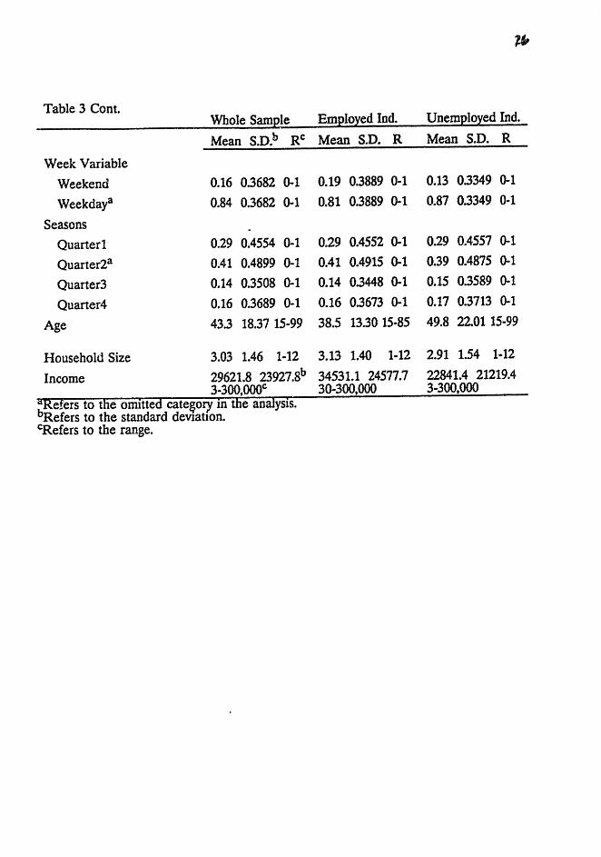
Table 3 Cont.

Week Variable Weekend Weekdaya

Seasons Quarter 1

Quarter2a

Quarter3

Quarter4

Age

Whole Sample Employed Ind. Unemployed Ind.

Mean S.D.b RC Mean S.D. R Mean S.D. R

0.16 0.3682 0-1 0.19 0.3889 0-1 0.13 0.3349 0-1

0.84 0.3682 0-1 0.81 0.3889 0-1 0.87 0.3349 0 .. 1

0.29 0.4554 0-1 0.29 0.4552 0-1 0.29 0.4557 0-1

0.41 0.4899 0-1 0.41 0.4915 0-1 0.39 0.4875 0-1

0.14 0.3508 0-1 0.14 0.3448 0-1 0.15 0.3589 0-1

0.16 0.3689 0-1 0.16 0.3673 0-1 0.17 0.3713 0-1

43.3 18.37 15-99 38.5 13.30 15-85 49.8 22.01 15 .. 99

Household Size 3.03 1.46 1 .. 12 3.13 1.40 1 .. 12 2.91 154 1·12

34531.1 24577.7 22841.4 21219.4 Income 29621.8 23927.8b

3-3oo,oooc ~Refers to the omitted cate~ory in the analysis. Refers to the standard dev1atlOn.

cRefers to the range.

30-300,000 3-300,000

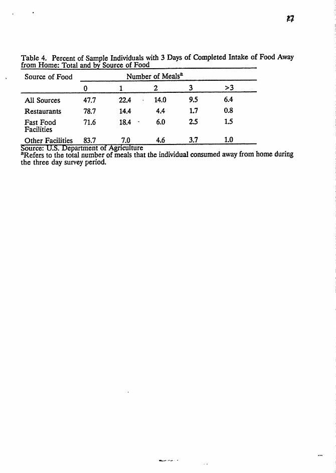
Table 4. Percent of Sample Individuals with 3 Days of Completed Intake of Food Away from Home: Total and by Source of Food

Source of Food

All Sources Restaurants

Fast Food Facilities

o 47.7

78.7

71.6

Number of Meals8

1

22.4

14.4

18.4 .

2

14.0

4.4

6.0

3

9.S 1.7

25

>3

6.4 0.8 1.S

Other Facilities 83.7 7.0 4.6 3.7 1.0 Source: U.S. Department of Agnculture aRefers to the total number of meals that the individual consumed away from home during the three day survey period.

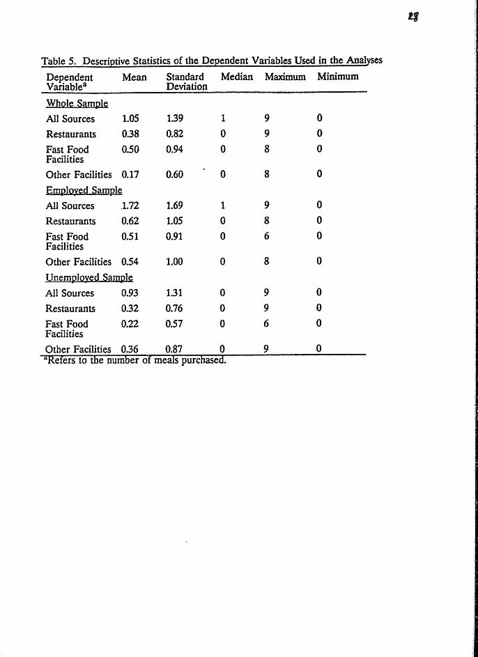
Table 5. Descrietive Statistics of the Deeendent Variables Used in the Analyses

Dependent Mean Standard Median Maximum Minimum Variablea Deviation

WbQl~ Silm~l~

All Sources 1.05 1.39 1 9 0

Restaurants 0.38 0.82 0 9 0

Fast Food 0.50 0.94 0 8 0 Facilities

Other Facilities 0.17 0.60 0 8 0

EmlllQ):~d Silml21~

All Sources .1.72 1.69 1 9 0

Restaurants 0.62 1.05 0 8 0

Fast Food 0.51 0.91 0 6 0 Facilities

Other Facilities 0.54 1.00 0 8 0

Unem12IQ):~d Silm121~

All Sources 0.93 1.31 0 9 0

Restaurants 0.32 0.76 0 9 0

Fast Food 0.22 0.57 0 6 0 Facilities

Other Facilities 0.36 0.87 0 9 0 3Refers to the number of mealS purchased.

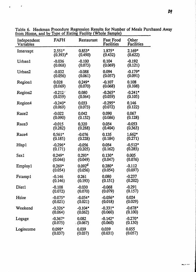
Table 6. Heckman Procedure Regression Results for Number of Meals Purchased Away from Home! and b~ Type of Eating Facility (Whole Sarne1e}

Independent FAFH Restaurant Fast Food Other Variables Facilities Facilities

Intercept 2.551· 0.853· 1.875· 2.169· (0.393)a (0.490) (0.432) (0.622)

UrbanI .. 0.036 -0.100 0.104 -0.192 (0.068) (0.073) (0.069) (0.121)

Urban2 -0.032 -0.088 0.094 -0.179· (0.056) (0.061) (0.057) (0.091)

Regionl 0.028 0.249· -0.107 0.108 (0.069) (0.070) (0.068) (0.108)

Region2 -0.212" 0.080 -0.265* -0.241* (0.059) (0.064) (0.059) (0.105)

Region4 -0.240· 0.033 -0.295· 0.146 (0.069) (0.073) (0.072) (0.122)

Race2 -0.022 0.042 0.090 0.067 (0.090) (0.132) (0.086) (0.128)

Race3 -0.015 0.320 0.054 -0.053 (0.282) (0.288) (0.404) (0.363)

Race4 0.561- -0.076 0.135 1.662· (0.185) (0.228) (0.184) (0.271)

Hispl -0.296· -0.056 0.054 .. 0.512· (0.171) (0.205) (0.162) (0.285)

Sexl 0.249· 0.293· 0.130· 0.005 (0.046) (0.049) (0.047) (0.076)

Employl 0.269· 0.092d 0.280· .. 0.112 (0.054) (0.056) (0.054) (0.097)

Fstampl -0.146 0.261 0.080 -0.237 (0.146) (0.193) (0.151) (0.202)

Dietl -0.108 -0.030 -0.068 -0.291 (0.072) (0.070) (0.079) (0.157)

Hsize -0.075· -0.054· -0.056· 0.024 (0.021) (0.021) (0.018) (0.029)

Weekend -0.326· .. 0.104· -0.331· -0.678· (0.064) (0.062) (0.060) (0.100)

Logage -0.367- 0.082 -0.142* -0.270· (0.075) . (0.067) (0.060) (0.130)

Logincome 0.09S- 0.039 0.039 0.055 (0.037) (0.037) (0.031) (0.057)

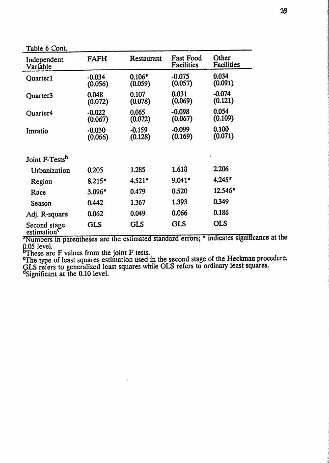
Table 6 Cont.

Independent FAFH Restaurant Fast Food Other Variable Facilities Facilities

Quarter! ·0.034 0~106* .. 0.075 0.034 (0.056) (0.059) (0.057) (0.091)

Quarter3 0.048 0.107 0.031 -0.074 (0.072) (0.078) (0.069) (0.121)

Quarter4 -0.022 0.065 "()~O98 0.054 (0.067) (0 .. 072) (0.067) (0.109)

Imratio -0.030 -0.159 -0.099 0.100 (0.066) (0.128) (0.169) (0.071)

Joint F-Testsb

Urbanization 0.205 1.285 1.618 2206

Region 8.215° 4.521111 9.0418 4.245·

Race 3.096· 0.479 0.520 12.546·

Season 0.442 1.367 1.393 0.349

Adj. R-square 0.062 0.049 0.066 0.186

Se~ond .staee GLS GLS GLS OLS estlmatlon

aNumbers in parentheses are the estlmated standard errors; • indicates significance at the ~ level.

ese are F values from the joint F tests. cThe type of least squares estimation used in the second stage of the Heckman procedure. ~LS refers to generalized least squares while OLS refers to ordinary least squares. Significant at the 0.10 level.

· . 26

Table 7. Heckman Procedure Re~ession Results for Number of Meals Purchased Away from Home b:l EmQloyed Individuals

Independent FAFH Restaurant Fast Food Other Variables Facilities Facilities

Intercept 2.782- 0.708 2.174· 3.630* (0.537)3 (0.543) (0.580) (0.995)

UrbanI 0.004 -0.106 0.073 -0.199· (0.090) (0.092) (0.088) (0.097)

Urban2 -0.003 -0..125 0.072 -0.050 (0.073) (0.077) (0.069) (0.079)

Region1 -0.019 0.091 -0.031 0.171-(0.089) (0.087) (0.084) (0.092)

Region2 -0.277· -0.066 -0.173* -0.085 (0.079) (0.079) (0.073) (0.084)

Region4 -0.251- -0.179· -0.226$ 0.233-(0.090) (0.090) (0.087) (0.095)

Race2 -0.029 0.005 0.128 0.189 (0.113) (0.136) (0.106) (0.116)

Race3 0.013 0.114 0.486 -0.369 (0.360) (0.315) (0.629) (0.340)

Race4 0.070 .. 0.032 0.290 -0.138 (0.255) (0.283) (0.222) (0.277)

Hispl -0.233 0.014 -0.022 0.170 (0.208) (0.233) (0.195) (0.220)

Sex1 0.166* 0.143· 0.166· 0.042 (0.059) (0.060) (0.056) (0.063)

Fstampl 0.236 -0.191 0.207 0.556· (0.254) (0.300) (0.283) (0.262)

Dietl .. 0.244- 0.022 .. 0.062 .. 0.274-(0.098) (0.094) (0.104) (0.111)

Hsize -0.155· -0.053· -0.036· -0.045-(0.026) (0.024) (0.021) (0.023)

Weekend -0.238- -0.354- -0.235· -0.337· (0.089) (0.076) (0.069) (0.080)

Logage -0.617· 0.050 -0.218· -0.190-(0.109) (0.089) (0.088) (0.095)

Logincome 0.263* 0.090· 0.022 -0.020 (0.047) (0.052) (0.042) (0.043)

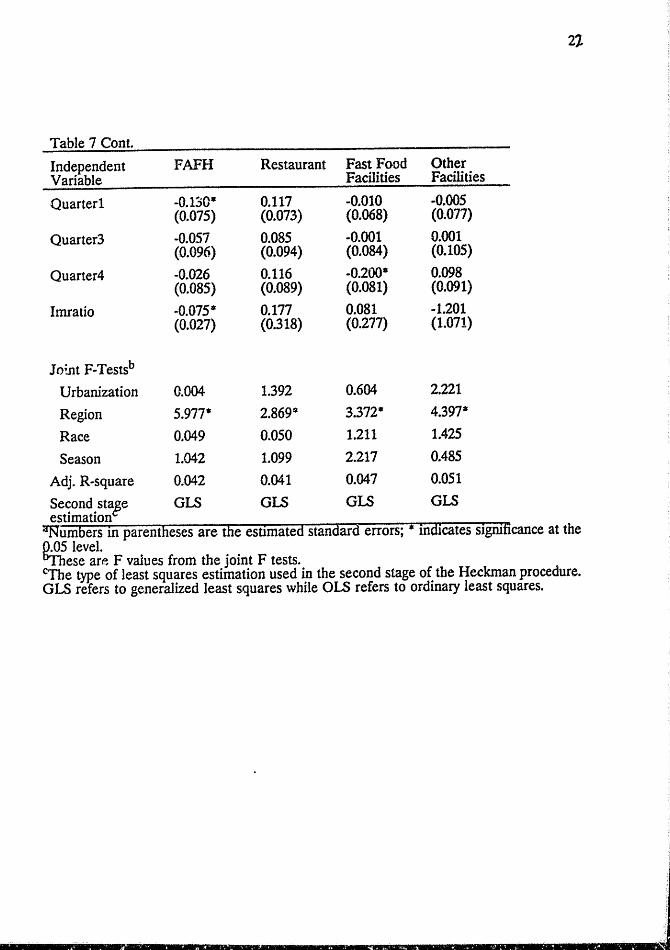
Table 7 Cont.

Independent FAFH Restaurant Fast Food Other Variable Facilities Facilities

Quarter! -0.130· 0.117 -0.010 -0.005 (0.075) (0.073) (0.068) (0.077)

Quarter3 -0.057 0.085 -0.001 OJlOl (0.096) (0.094) (0.084) (0.105)

Quarter4 -0.026 0.116 -0.200· 0.098 (0.085) (0.089) (0.081) (0.091)

Imratio -0.075· 0.177 0.081 ... 1.201 (0.027) (0.318) (0.277) (1.071)

Jomt F-Testsb

U rbanizatioll 0.004 1.392 0.604 2.221

Region 5.977· 2.869$ 3.372- 4.397·

Race 0.049 0.050 1.211 1.425

Season 1.042 1.099 2.217 0.485

Adj. R-square 0.042 0.041 0.047 0.051

Se~ond. staee GLS GLS GIS GIS estImation ~umbers In parentheses are the estimated standard errors; • indicates sigruficance at the ~ level.

ese an~ F values from the joint F tests. Ofhe type of least squares estimation used in the second stage of the Heckman procedure. GLS refers to generalized least squares while OLS refers to ordinary least squares.

- .• j • =

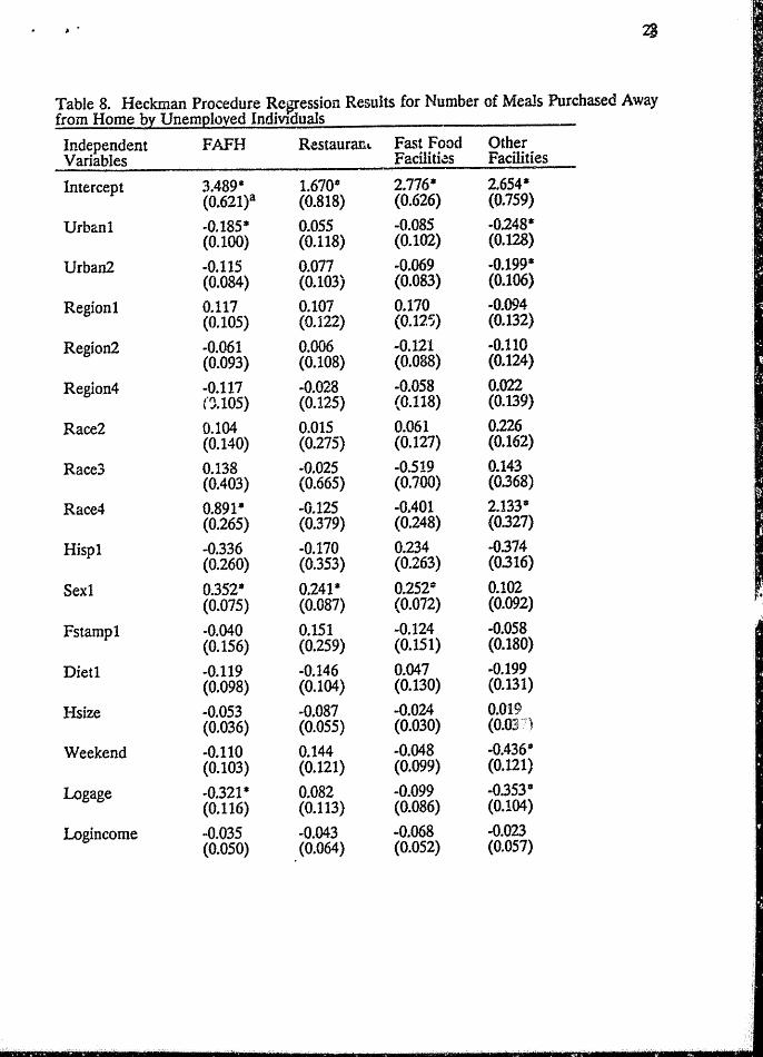
Table 8. Heckman Procedure Re~ession Results for Number of Meals Purchased Away from Home b~ UnemQlo:ied IndiVIduals

Independent FAFH Rcstaurart&. Fast Food Other Variables Facilities Facilities

Intercept 3.489* 1.670· 2.776* 2.654-(0.621)a (0.818) (0.626) (0.759)

UrbanI -0.185· 0.055 -0.085 -0.248-(0.100) (0.118) (0.102) (0.128)

Urban2 -0.115 0.077 -0.069 -0.199· (0.084) (0.103) (0.083) (0.106)

Region1 0.117 0.107 0.170 .. ()'094 (0.105) (0.122) (0.12;) (0.132)

Region2 -0.061 0.006 -0.121 .. 0.110 (0.093) (0.108) (0.088) (0.124)

Region4 -0.117 .. 0.028 .. 0.058 0.022 {~.105) (0.125) {C. I 18) (0.139)

Race2 0.104 0.015 0.061 0.226 (0.140) (0.275) (0.127) (0.162)

Race3 0.138 -0.025 -0..519 0.143 (0.403) (O.665) (0.700) (0.368)

Race4 0.891· -0.125 -00401 2.133· (0.265) (0.379) (0.248) (0.327)

Hispl -0.336 -0.170 0.234 -0.374 (0.260) (0.353) (0.263) (0.316)

Sex! 0.352* 0.241· O.252c 0.102 (0.075) (0.087) (0.072) (0.092)

~

1

Fstampl -0.040 0.151 -0.124 ·0.058 (0.156) (0.259) (0.151) (0.180)

Dietl -0.119 -0.146 0.047 -0.199 (0.098) (0.104) (0.130) (0.131)

Hsize .. 0.053 -0.087 .. 0.024 0.019 (0.036) (0.055) (0.030) (0.03

Weekend .. 0.110 0.144 -0.048 .. 0.436" (0.103) (0.121) (0.099) (0.121)

Logage .. 0.321· 0.082 .. 0.099 -0.353* (0.116) (0.113) (0.086) (0.104)

Logincome .. 0.035 -0.043 -0.068 .. 0.023 (0.050) (0.064) (0.052) (0.057)

29

Table 8 Cont.

Independent FAFH Restaurant Fast Food Other Variable Facilities Facilities

Quarterl 0.091 -0.005 -0.098 0.065 (0.089) (0,101) (0.084) (0.110)

Quarter3 0.151 0.137 0.028 0.074 (0.111) (0.131) (0.101) (0.140)

Quarter4 0.238* 0.063 -O<O~O 0.347* (0.105) (0.122) (0.101) (0.132)

Imratio 0.063 -0.021 -0.335 0.766* (0.072) (0.336) (0.240) (0.384)

Joint F-Testsb

Urbanization 1.832 0.290 0.464 2.566*

Region 1.407 0.382 1.913 0.475

Race 3.879* 0.038 1.198 14.52·

Season 1.884 0.477 0.637 2.350

Adj. R-square 0.063 0.046 0.079 0.186

Se~ond. staee GLS GLS GLS GLS estImatIon

aNumbers in parentheses are the estunated standard errors; • indicates significance at the ~ level.

ese are F values from the joint F tests. CJbe type of least squares estimation used in the second stage of the Heckman procedure. GLS refers to generalized least squares while cLS refers to ordinary least squares.