Impact of Mergers on the Degree of Competition in the ... · competition in the banking industry ex...

1

Impact of Mergers on the Degree of Competition in the Banking Industry

Vittoria Cerasi†, Barbara Chizzolini‡ and Marc Ivaldi§

This version: 10 August 2013

Abstract: In this paper we propose a new test for evaluating the impact of horizontal mergers on competition in the banking industry ex ante. The test is based on a monopolistic competition model where firms compete on price and branching, and market structure is endogenous. Using a Maximum Likelihood approach, we fit the branching behavior of French and Italian banks and obtain an estimated measure of competition in local markets for two alternative cases: the pre-merger case, in which the number and branching networks of incumbent banks in each market is the one actually observed; the post-merger case, where we simulate horizontal mergers between incumbent banks. Estimated measures of competition in the two cases are then compared. We provide examples of mergers that are either favorable or detrimental to market competition. Our empirical test can be useful in competition analysis. Thanks to its theoretical foundation, it encompasses more information than traditional measures of concentration, while being as parsimonious as the Herfindahl index in terms of data requirements. JEL classification: G21 (Banks); L13 (Oligopoly); L59 (Regulation and industrial policy). Keywords: Banking industry; Competition and market structure; Merger policy. Acknowledgements: We thank Rosella Creatini, Wolf Wagner, Sub Ramanarayanan and Jung-Hyun Ahn for helpful discussions and participants, among others Stijn Ferrari, Peter Davis, Thorsten Beck, Elu Von Thadden, Hans Degryse and Robert Marquez at the ACE Workshop on Antitrust and Regulation, Fondazione Eni Enrico Mattei, Milan (October 2009), 2nd CEPR-EBC-UA Conference on competition in banking markets, Antwerp (December 2009), ZEW Conference on Quantitative Analysis in Competition Assessments, Mannheim (October 2010), FEBS 2012 Conference on Recent Developments in Financial Markets and Banking, London (June 2012) and 16th Centre for Competition and Regulatory Policy Workshop, Milan (July 2013). Chizzolini acknowledges V. Chiorazzo and C. Milani at ABI for useful comments and for providing data on Italian banking groups and Ente L. Einaudi for financial support, while Cerasi acknowledges financial support from Fondo di Ateneo per la Ricerca (FAR) from Bicocca University. † Corresponding author: Department of Economics, Management and Statistics (DEMS), Bicocca University, Piazza dell’Ateneo Nuovo 1, 20126 Milan (Italy), [email protected], phone: +39-02-6448.5821, fax. +39-02-6448.5878. ‡ Department of Economics, Bocconi University, via Roentgen 1, 20136 Milan (Italy), [email protected] § TSE Université de Toulouse Capitole, Manufactur des Tabac - Bâtiment F, Allée de Brienne, 31000 Toulouse (France), [email protected]

2

1. Introduction

Horizontal mergers are considered detrimental to competition, since concentration and

competition are usually considered to be as inversely related. Although at the forefront for many

years, the debate in applied industrial organization about competition and concentration (see for

instance the survey in Schmalensee, 1989) has failed to produce compelling evidence. The issue is

particularly critical in banking, where concentration and competition may not only affect the

profitability of each individual bank, but the stability of the overall industry as well (see Degryse

and Ongena, 2008, and Carletti and Vives, 2009 among others).

And yet, there is no conclusive evidence that mergers always reduce competition, as one

side of the literature predicts. In some instances, the opposite may occur. For example, when market

structure is fragmented with the exception of a single dominant firm, a horizontal merger between

medium-sized players might restore competitive conditions by generating a rival for the incumbent.

In this case, greater concentration in market share is accompanied by greater competition, breaking

down the inverse relation between concentration and competition (as argued by Cetorelli, 1999,

Berger et al., 2004, and Dick, 2007). In this case, the use of traditional measures of concentration to

infer the degree of competition when conducting merger analysis, such as for instance the

Herfindahl–Hirschman Index (HHI, thereafter), may be misleading.

The objective of this paper is to provide, within the extant debate, a measure of competition

to account for structural changes following M&As among banks. This measure is derived from a

model where competition and market structure are simultaneously determined, and it is estimated

by using publicly available data, the same that antitrust authorities normally use in their

assessments. We provide evidence that some mergers, while increasing concentration, do not

necessarily reduce the degree of intra-industry competition. In some cases, by increasing the

number of larger players, mergers may even enhance competition.

More specifically, within a model of monopolistic competition where incumbent banks

compete by setting interest rates and establishing branching networks, we apply a latent variable

approach à la Bresnahan-Reiss (1991a, 1991b) to infer branching costs and revenues in local

markets from the observed branching behavior of banks. We interpret the elasticity of estimated

profits with respect to branching as a new indicator of the degree of competition in the industry:

tougher rivalry over interest rates reduces this elasticity, thus revealing greater competition. The ex-

ante effect of horizontal mergers on competition is captured by comparing the value of this

elasticity in the pre- and post-merger market structures. First, we estimate our model by using the

actual pre-merger number of banks and their branching size. Then we estimate it a second time

3

under a virtual scenario where we simulate a merger which adds and combines the branches of

potentially merging banks, while keeping the branches of other incumbent banks constant. We show

that competition, as captured by our measure, is not only affected by the degree of market

concentration, but also by the dispersion of market share and by the number of large players in the

industry.

We apply our test to the Italian and French banking industries. In both countries the number

and size of incumbent banks have substantially changed over recent years, due to the occurrence of

several horizontal mergers. It is interesting to study the two banking industries together because of

the significant differences in their pre-merger structures. In France, all major banking groups

compete against each other in all local markets. In Italy, only a few banking groups operate at the

national level, while the majority of actors are local banks, implying that each bank faces a different

set of competitors in every single local market. These two industries provide examples of mergers

that potentially have contrasting effects in terms of competition.

As an application, we simulate the mergers between Crédit Agricole and Crédit Lyonnais

and between Crédit Mutuel and Crédit Industriel Commercial in France, and two of the most

important mergers to have occurred in Italy in recent years, the one between Intesa and Sanpaolo

IMI, and the one between UniCredit and Capitalia. Our competition indicator detects opposite

effects for these mergers: they turn out to be pro-competitive in France, and anti-competitive in

Italy. In France, in most local markets those mergers have created at least a new bank, big enough

to compete with incumbent dominant banks. In Italy, on the contrary, the two mergers have reduced

the number of big players, in some local markets, at least.

These results cannot be fully captured by considering the change in market concentration in

isolation, even locally, since in both cases the HHI rises. In addition our measure of competition is

parsimonious in terms of required information, since it only uses data on branching market shares of

individual banks in local markets, without using accounting data, even when publicly available at

this level of disaggregation. These are the same informational requirements used to compute the

HHI, which is the measure of concentration most commonly used in antitrust analysis. Finally, our

approach, although here applied to retail banks, can be easily transferred to other industries that use

retail networks for the sale of a final product, as for instance the insurance industry, grocery chain

stores, car dealers, or even to industries where firms operate on the market through a single branch,

such as professionals like doctors or lawyers.

In Section 2 we review the main references in the literature; in Section 3 we derive the

econometric model from the banks’ branching behavior with the objective of measuring the degree

4

of competition in local markets. Then the results of econometric testing applied to individual banks’

data in local markets are presented in Section 4. Section 5 is devoted to the simulation of a few

horizontal mergers, to examine their impact on the degree of competition; finally we discuss the

relation between our estimated measure of competition and other measures of concentration.

Section 6 concludes the paper.

2. Review of the literature

This paper is related to the empirical literature on the industrial organization of endogenous

market structure that departs from Bain (1956), as thoroughly discussed in Sutton (1991). More

specifically, this paper is related to studies measuring competition in retail markets that use

structural models of monopolistic competition. To derive branching costs from observed choices of

branching, we follow the latent variable approach adopted by Bresnahan and Reiss (1991a, 1991b),

and subsequently refined by Berry and Tamer (2006). Their idea is that, by observing the presence

of a firm in a market, it is possible to uncover information about entry costs. We apply this same

logic to branching choices: by virtue of its presence in a market with a given number of branches, a

bank reveals that it expects to recover the costs of a branching network of that size. Therefore we

derive information about the non-observable cost of branching by observing branch presence in a

given market. Our paper exploits this result to study the changes in market structure following a

merger, and to measure its impact on the degree of competition.

In a recent paper Schaumans and Verboven (2011) estimate a measure of change in

competition within a model with differentiated products, and apply it to the local services markets.

They estimate an ordered probit entry model, as in Bresnahan and Reiss (1991a, 1991b), jointly

with an industry revenue function to obtain a competition measure. Their approach is close in its

objective to ours, but it imposes heavier data requirements compared to our test. This is why we

think it cannot be easily adapted to industries characterized by a large number of either firms or

branches, as in our case.

In that body of literature there is a further potential problem of identification: profits and

sunk costs are in fact estimated up to a monotonic transformation. We have solved it here by

introducing a measure of competition that only affects profits without affecting branching costs. In

this way we are able to estimate directly a measure of the degree of competition.

Based on the idea that firms in more competitive markets suffer from larger decreases in

profits when their costs increase, Boone (2008) and Boone et al. (2007) have proposed a measure of

5

competition that captures the elasticity of accounting profits to costs. We use a similar idea by

proposing the elasticity of profits to branching as a measure of competition. In contrast to those

papers, however, our measure of competition does not require any prior knowledge of accounting

data. Cohen and Mazzeo (2007) propose a model of monopolistic competition where they estimate

the competitive response of banks to different types of branching behavior. Our approach is similar,

since we both estimate directly the structural equations to infer non-observable branching costs;

however we improve on this approach, by exploiting the model to simulate the impact of horizontal

mergers on the measure of competition.

This paper springs from preliminary articles where the markets considered were,

respectively, the Italian provinces between 1989 and 1995 in Cerasi et al. (2000) and the national

industries of several European countries before and after the implementation of the Second

European Directive in 1992 in Cerasi et al. (2002). We have exploited the same econometric

methodology to fit the model on two countries, France and Italy, but using data of higher quality

and making improvements on our methodology by suggesting a way to simulate the impact of

horizontal mergers between incumbent banks on our measure of competition.

The simulation of mergers based on a structural model of monopolistic competition departs

from other papers in the literature where the impact measurement is carried ex post based on

accounting data, i.e. after mergers have actually occurred (see applications to the banking industry

in Molnar, 2008, and Zhou, 2008). In those papers, the exercise consists in estimating demand and

supply parameters before the merger, and subsequently using estimated coefficients to simulate a

change of ownership in the allocation of the branches with the purpose of assessing the impact on

competition (as surveyed in Budzinski and Ruhmer, 2010). Our objective is similar in that we

derive an impact assessment before the merger occurs, but without imposing heavy data

requirements other than the information needed to compute the HHI at the local market level. We

believe that our method provides useful guidance to competition authorities who have to assess the

impact of mergers in the banking industry ex ante. The ex-ante assessment provides a method to

reject or approve a specific merger, while the ex-post assessment aims at evaluating the change in

market structure by taking into account also the reaction by rivals once the merger has already been

approved. The two approaches, ex-ante and ex-post, provide complementary ways to formulate an

assessment of mergers.

We apply our approach to the banking industry. There are several papers that study the

impact of horizontal mergers of banks on market structure (Sapienza, 2002 and Focarelli and

Panetta, 2003; to cite just a few). All these papers apply the ex-post approach on data of finer

6

quality, by using Credit Register’s information on the banks’ portfolios of loans. However their

evidence on the effect of mergers on banks’ market power is mixed.

3. Defining a measure of competition

In this section we propose an empirical measure of the degree of competition in banking

services at the local level, derived from the observed behavior of banks in local markets.

Here is the rationale for our analysis. Banks compete for clients by opening branches in

specific local markets and then setting the price of a bundle of financial services.1 A bank enters a

local market whenever its expected gross profits cover the cost of entry, and the size of its

branching network is chosen by equating the marginal revenue of an additional branch with its

marginal cost. In formal terms, let us define πij the gross profit of bank i in market j . Gross profits,

i.e. the revenues of a branching network without accounting for costs, must be an increasing

variable with respect to the number of branches in market j, kij, otherwise we would never observe a

bank opening new branches. However the increase in bank’s gross profits due to an additional

branch is the result of the balance of two contrasting effects: i) a positive (“expansion”) effect, if the

new branch is successful in attracting new clients and earns new revenues, and ii) a negative

(“competition”) effect, if the new branch steals clients from pre-existing branches of the same bank.

The overall effect of an increase in branching size is captured by the notion of elasticity of gross

profits to branching, formally ��

. Notice that this elasticity is indeed affected by the degree of

competition in that market. When the gains from opening an additional branch in a local market are

large, we infer that banks in that market are facing softer competition for new clients. To

summarize, greater competition for banking services in market j is reflected by a lower elasticity of

profits to branching. This expression uncovers our strategy to measure competition in market j, that

is, we approximate the degree of price competition in banking services by measuring the inverse

elasticity of gross profits to branching.

There are other factors affecting bank profits. First of all, the level of profits of bank i in

market j must be increasing in total market size Sj. Market size represents a demand shifter that

captures the maximum reservation value consumers are willing to pay for banking services. Note

that, for a given market size S, a larger profit implies lower consumers’ surplus. Also the total

1 Branching is still important in retail markets since geographic proximity represents a competitive advantage when

monitoring loans to opaque SMEs or when supplying deposits, as argued in Petersen and Rajan (2002), Degryse and Ongena (2005), Brevoort and Hannan (2006) and Dick (2007).

7

number of branches Nj in market j affects bank profits: as the market becomes crowded with other

banks’ branches, the additional profit of a new branch shrinks.

Expressing all this in formal terms, bank i gross profit in market j is:

�� , �� , �� (1)

The marginal benefit of an additional branch MBij is the derivative of the function (1) with

respect to kij holding constant all branches by rival banks i.e. �� ∑ �� .

Banks choose their optimal branching size by setting the marginal benefit of an additional

branch MB equal to the marginal cost MC of branching. To keep matters as simple as possible, we

assume that an additional branch has a fixed marginal cost MCij.2 As summarized in Box 1 each

bank sets its branching network size at * 1ijk > according to Equation (2a), by equating the marginal

benefit of an additional branch to its marginal cost; otherwise it sets * 1ijk = and Equation (2b) holds.

In addition, the free entry condition requires that a bank enters market j up to the point where its

expected gross profits are equal to the entry cost3 for a given branching size as stated by Equation

(3).

Box 1 – Choice of branching size and entry decision

Branching size choice: * 1ij ij ijMB MC k= ⇒ > (2a)

* 1ij ij ijMB MC k< ⇒ = (2b)

Entry decision: ijij σπ ≥ (3)

where kij is the number of branches and sij is the entry cost of bank i œ{1,…, n} in local market jœ{1,…,J}.

Note that the marginal benefit of branching can be related to the elasticity of gross profits to

branching, since ��

��

. A greater degree of competition in the price of banking services,

that is, a lower elasticity, reduces MB. Note that the degree of competition affects the marginal

benefits of branching, while it does not change marginal cost MC, assumed constant. In our

framework, tougher price competition has a negative impact on branching size, ceteris paribus. For

a given market size and number of competitors, if competition gets tougher (lower elasticity of

gross profits to branching) a bank may end up closing branches (*k will decrease in (2a)) since the

expected gains from a larger branching network shrink.

The major advantage of this approach is that it requires a very limited amount of information

to recover bank and branch profitability, i.e. we just need to know the number of branches of each

2 This is not the marginal cost of producing banking services, but the unit cost of opening a new branch. This cost is specific to each bank in each local market. 3 Given that we do not observe new entries in any of the markets, this condition is redundant and we will not use it in

the econometric implementation.

8

bank in a specific local market: this is publicly available information. We can list several reasons as

to why it is convenient to use this approach. First, these are easily accessible data even at the

disaggregate level, while instead we lack accounting records for profits at the local market level for

banks that are simultaneously active in several markets. Second, merger analysis uses the measure

of the HHI derived from market shares with respect to branches, in order to detect potential

restrictions to competition; our framework uses precisely the same data, without requiring

additional information. Finally, in addition to the number of branches in a specific market we may

also observe its evolution over time: this information is crucial to measure expected long-term

profitability. Since the opening and closing of branches is a costly affair, a bank opens new

branches only when it expects to recover the cost of its branching network through additional

profits in the future. This profitability, although affected by contingent macroeconomic factors,

depends also upon long-lasting features of market structure, such as the number of competitors,

market size etc. Thus a measure that uses information implicit in the size of branching networks

aims to capture also the idea of long-term profitability within a specific market structure.

3.1. Econometric specification

To derive branching costs from observed choices of branching, we follow the latent variable

approach. We assume that the latent marginal costs of branching explain observed branching

decisions. Exploiting the variation in the number of branches of individual banks, we can retrieve

not only marginal branching costs, but also the degree of competition in each market that is

compatible with observed changes in the size of branching networks.

The objective is to write a likelihood function for our observations in terms of branching

behavior. From the previous section we know that either one of the two branching Conditions (2a)

or (2b) must hold, once we assume that banks instantaneously adjust the optimal size of their

branching networks in each period and market. We classify each observation (ijt ), namely bank i in

period t in local market j, into one of the following four categories:

[a] “expanding multi-branch” bank if Dkij t= (kij t-kij t-1) > 0 and kij t >1;

[b] “static multi-branch” bank if Dkij t= 0 and kij t >1;

[c] “shrinking multi-branch” bank if Dkij t < 0 and kij t >1;

[d] “unit-branch bank if Dkij t= 0 and kij t =1.

Note that, at time t, for multi-branch banks included in cases [a] to [c], Condition (2a), i.e. marginal

branching benefits equal marginal branching costs, must hold, while for unit-branch banks of case

9

[d], Condition (2a) is replaced by Condition (2b): marginal branching benefits must be lower than

marginal branching costs.

For the purpose of the econometric estimation we choose a specific functional form4 for the

profits of bank i in market j (omitting time t) which satisfies the properties of the function described

in the previous section, namely:

�� , �� , ��

��

�� (4)

This functional form exhibits the coefficient cci, the elasticity of gross profits to branching

and our inverse measure of competition, as an explicit coefficient in the formula.5 To exploit the

observed changes in the size of branching networks, we replace MBijt with Aijt inside the branching

Conditions (2a) and (2b):

��

��

��!""#��

$��% (5)

which is a slightly modified formula with respect to MB, where instead of the number of branches at

time t, kijt, we use its lagged value kijt-1 inside the brackets. It follows that: when kijt-1<kijt, then

Aijt>MBijt for the expanding multi-branch banks in case [a]; when kijt-1>kijt, then instead Aijt<MBijt

for shrinking multi-branch banks in case [c]; while Aijt=MBijt for static multi-branch banks in [b]

and for unit banks in [d], neither of which changes the size of its branching network in the observed

time span. It also follows that in the modified Condition (2a), the equality between MBijt and MCijt

is substituted by the inequality between Aijt and MCijt for all banks falling in cases [a] and [c].

Specifically Aijt>MCijt for expanding banks, and Aijt<MCijt for shrinking banks.

These modified conditions yield a simplified partitioning of observed banks into two

subsets:6

&'�: )** +), - #, .)/ ),0 .+/ -1 23)2 �� 4 �5�� (6)

&$�: )** +), - #, ."/ ),0 .0/ -1 23)2 �� 6 �5��

To cast each observation in the probability space, we assume that the marginal branching cost for

bank i in market j at time t is a random variable with known probability distribution. More

specifically, we assume that the distribution is lognormal and that the logarithm of costs has a mean

different from zero:

4 In the econometric exercise we tested other functional forms without obtaining relevant differences in terms of results. 5 The elasticity of profits with respect to branches is given by 7""# � �

$�8 and as N increases the elasticity collapses to

cci. 6 Since we have made an arbitrary choice when allocating the “static multi-branch” banks in the sub-set E1t, we will check the robustness of our results to a different classification criterion in the next section.

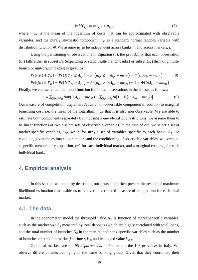
10

*,�5�� 9"�� : ;��, (7)

where mcijt is the mean of the logarithm of costs that can be approximated with observable

variables, and the purely stochastic component, uijt, is a standard normal random variable with

distribution function Φ. We assume uijt,to be independent across banks, i, and across markets, j.

Using the partitioning of observations in Equation (6), the probability that each observation

(ijt ) falls either in subset E1t (expanding or static multi-branch banks) or subset E2t (shrinking multi-

branch or unit-branch banks) is given by:

<=>?#@2A B &'�C � <=��5�� D �� <=�;�� D *,�� 9"�� Φ�*,�� 9"�� (8)

<=>?#@2A B &$�C � <=��5�� F �� <=�;�� F *,�� 9"�� 1 � Φ�*,�� 9"��

Finally, we can write the likelihood function for all the observations in the dataset as follows:

H � ∑ *,Φ�*,�� 9"��?��ABI � : ∑ *,J1 � Φ�*,�� 9"��K?��ABIL (9)

Our measure of competition, ccijt enters Aijt as a non-observable component in addition to marginal

branching cost, i.e. the mean of the logarithm, mcijt that it is also non observable. We are able to

estimate both components separately by imposing some identifying restrictions: we assume them to

be linear functions of two distinct sets of observable variables. In the case of ccijt we select a set of

market-specific variables, Wjt, while for mcijt a set of variables specific to each bank, Zijt. To

conclude, given the estimated parameters and the conditioning of observable variables, we compute

a specific measure of competition, cci, for each individual market, and a marginal cost, mc, for each

individual bank.

4. Empirical analysis

In this section we begin by describing our dataset and then present the results of maximum

likelihood estimation that enable us to recover an estimated measure of competition for each local

market.

4.1. The data

In the econometric model the threshold value Aijt is function of market-specific variables,

such as the market size Sjt measured by total deposits (which are highly correlated with total loans)

and the total number of branches Njt in the market, and bank-specific variables such as the number

of branches of bank i in market j at time t, kijt, and its lagged value kijt-1.

Our local markets are the 95 départements in France and the 103 provinces in Italy. We

observe different banks belonging to the same banking group. Given that they coordinate their

11

decisions on interest rates and branching, we decided to define the banking group rather than the

single bank as the appropriate unit of observation.7 Each observation therefore describes banking

group i operating in local market j at time t with given branching size kijt.8

We gathered information on the number of branches held by each banking group in every

local market in two years, 2005 and 2007 in France, and 2004 and 2006 in Italy. We computed ∆kijt,

that is the change in branching size for each group in each local market, taking 2005 as the initial

year for France, and 2004 for Italy.

For Italy, data on bank branches by provinces can be obtained from the public website of

Bank of Italy.9 For France, data on bank branches by departments were directly provided by Crédit

Agricole and Caisses d’Epargne. In France almost all banks have branches in all the 95

departments, with the only exception of C.I.C. that has no branches in Corsica. In Italy six national

banking groups control branches located in almost all 103 provinces, while the remaining groups

have branches geographically concentrated in few local markets. Descriptive statistics in Tables 1a

and 1b show that the two industries are quite different in terms of network size, with Italian banks

being smaller compared to French banking groups, since average branching size is 19 in Italy, while

it is 46 in France (median value is 7 in Italy compared to 23 in France). The total number of

branches for every local market is greater in France, although market shares are on average larger

indicating that several large players are simultaneously active in each market. The two countries are

more similar for what concerns the dispersion of branches within markets, as measured by standard

deviation.

[Insert Tables 1a and 1b here]

We do not rely on accounting data for our analysis. As a matter of fact accounting measures

of bank profits are rarely available at this level of disaggregation: accounting statements provide

balance sheet data at consolidated level, that is, aggregate across all markets in which the bank is

active. For instance, suppose that bank A owns branches in markets a and b: From its accounting

7 On the one hand, we exclude from the analysis small groups or independent banks since they do not behave

strategically but are price takers and adapt their branching behavior residually. They are nevertheless included in the denominator Nj, representing the total number of branches in that market, since they exert a competitive pressure on branches of the main groups in each local market by behaving like a fringe. On the other hand, we include La Poste among banking groups in France as the banking part of the French postal mail provider has a large and dispersed network. In contrast, Poste Italiane is excluded as it did not play at the time of our analysis a similar role. 8 To capture coordination among banks belonging to the same group across different local markets in our econometric analysis, we control for ownership by using a dummy variable specific to each group. This has also the advantage that we automatically account for other differences across banks, such as mutual vs. commercial banks without adding further dummies in the estimation. 9 The number of branches for individual banks are taken from www.bancaditalia.it, while we followed the ABI guidelines for the definition of banking groups.

12

statement we would be able to recover only consolidated profits across the two markets, not the two

profits separately, i.e. the profit of bank A in market a and profit of bank A in market b, as required

by our analysis to recover the competitive behavior of banks at local level. Luckily our empirical

strategy provides us with a simple proxy for bank’s profit in each market, as expressed by the

reduced form in Equation (4), which is a function of the market share of the bank in each local

market based on the number of branches.

Still our definition of a bank’s profits in each local market must be correlated with the actual

accounting profits. Consider that accounting profits are proportional to deposit or loan market

shares for retail banks. Since these are also highly correlated with branching market shares, we

expect a high correlation between our profits given by reduced form in Equation (4) and the

recorded accounting profits.

Finally, in the empirical specification of mci, we include Zit a dummy for each banking

group among explanatory variables. Our assumption is that a greater percentage of branching costs

is affected by the cost structure and the internal organization of the bank, rather than by the

characteristics of the market where the branch is located.10 The inverse measure of competition cci

instead depends upon a set of market-specific variables, Wjt, including per capita loans (LPC), the

proportion of rural areas in each county (SHRUR) in France, and a dummy indicating densely

populated urban areas (DBIGPRO) in Italy. These variables, taken from the two countries’ central

statistical agencies, INSEE for France and ISTAT for Italy, capture the expected level of activity of

all banks in a given local market. We expect to find tougher competition in markets with higher per

capita loans and more densely populated areas, due to the greater incentive to compete for the

marginal client when economic activity is more intense.

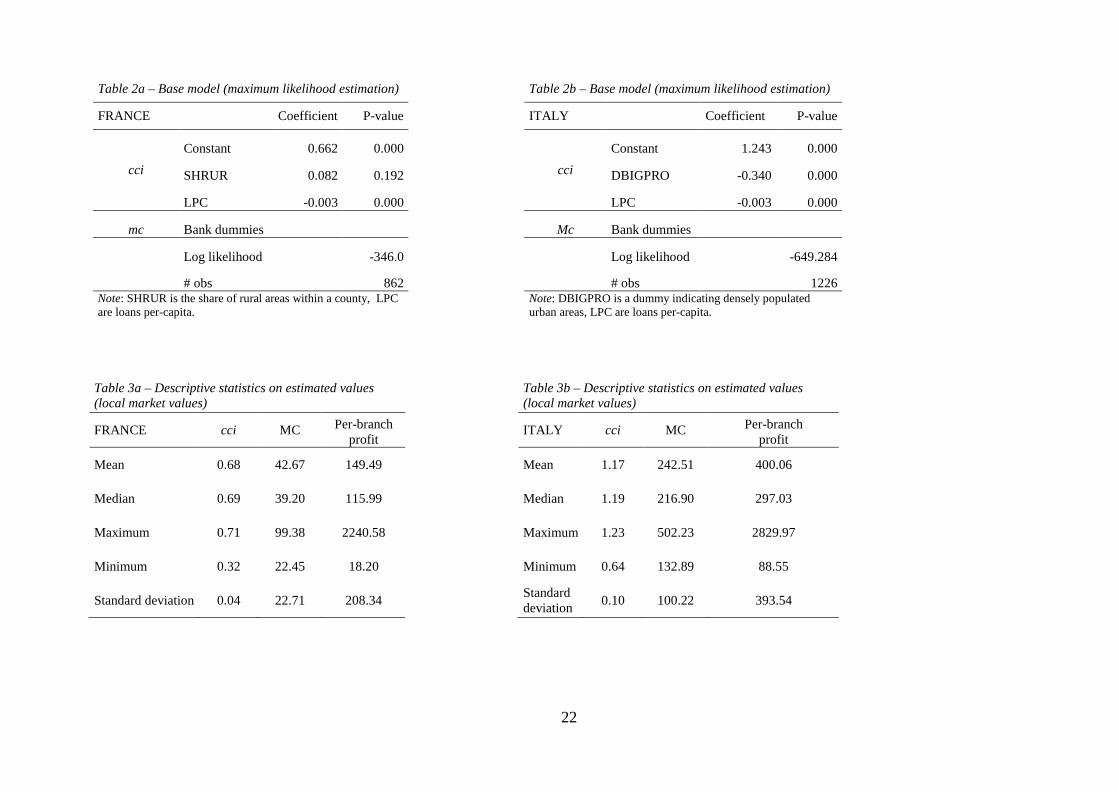
4.2. Maximum likelihood results

The econometric model is estimated for a cross-section of data covering year 2006 in Italy

and year 2007 in France. These results, defined the “base model”, will be confronted with the

results of the estimation simulating the mergers in the next section. All coefficients of the maximum

likelihood estimation in Tables 2a and 2b are significant, although differences in their values

capture local heterogeneity.

10 This assumption is supported by findings in Cerasi et al. (2002) where we show that variables such as the total number of employees and the distance of the branch from the location of bank’s headquarters significantly affect marginal branching costs. This implies that marginal branching costs depends upon variables specific to the bank rather than to each local market.

13


The signs of the coefficients associated to cci are in accordance with our intuition: a positive

sign indicates that competition is weaker (greater cci) in less densely populated areas in France,

measured by a greater incidence of rural areas (SHRUR), while in Italy competition is stronger

(smaller cci) in those provinces where we find a big city (DBIGPRO). In addition, in both countries

competition increases with the level of economic activity as measured by per capita loans (LPC).

Tables 3a and 3b show the differences in competition, branching costs and profitability

between the two countries. The mean value of cci, is higher in Italy at 1.17, when compared to

France, which has a value of 0.68 (lower values of cci imply stronger competition) meaning that

local markets are on average more competitive in France than in Italy. Marginal costs of branching

are lower in France than in Italy, and, moreover, they represent a smaller share of our estimated per

branch profits: the French banking system is not only more competitive but each branch costs less.


Tables 4a and 4b exhibit heterogeneity of estimated marginal branching costs across

banking groups, in particular Crédit Agricole and La Poste have higher branching costs and

considerably lower per-branch profits compared to rival French groups. These two groups are

indeed characterized by large branching networks spread all over the country, even in less densely

populated areas. Conversely, in Italy per branch profits are relatively more homogeneous across

banking groups, with higher marginal costs for UniCredit.


In Tables 8a and 8b (reported in the Appendix), we compile the ranking of local markets

using our estimated measure of competition. The parameter cci varies considerably across local

markets. In densely populated areas our measure cci takes smaller values indicating tougher

competition. For instance, in Paris cci reaches its lowest value. In Italy the overall variance of cci is

greater. Notice that cci takes lower values in most Italian Northern provinces compared to Southern

provinces. This result suggests that banks located in Northern regions face greater competition

compared to those located in Southern regions. (See Cerasi et al., 2000 and Guiso et al., 2006,

among others, for similar empirical evidence.)

Finally we provide an indication of how good is the econometric model in fitting the data. A

goodness-of-fit measure is obtained by comparing predicted branching behavior to the actual

partitioning of observations between subset E1 (all expanding multi-branch or static multi-branch

banks) and E2 (all shrinking multi-branch or unit-branch banks). Tables 5a and 5b report the

percentage of observations whose behavior in terms of branching is correctly predicted by the

model; namely, that it correctly forecasts the number of banks that should have opened new

14

branches and have indeed done so, and that it does the same for banks that should have closed some

of their branches or kept them unchanged: the percentage is 84% for France and 75% for Italy.11


5. Measuring the impact of mergers on competition

We now use our econometric model to simulate the impact on competition of specific

horizontal mergers between two or more banks. For a given merger, we undertake the following

exercise: we sum the branches of the merging banks in each local market where the banks are active

and re-estimate the model assuming that these new entities replace the old ones; we also assume

that rivals are passive, in the sense they don’t react to the merger by changing their branching size

in any of the local markets. Our econometric model yields the estimated degree of post-merger

competition. We then compare this new estimated measure of competition to the degree of

competition in the base model. By comparing the two cci, pre- and post-merger, we can say whether

the merger under evaluation is pro- or anti-competitive. An increase in our measure of competition

implies a reduction of per branch profit; for given market size S, this implies a larger surplus and

therefore from the consumers’ point of view the merger is beneficial.

We think that this exercise provides a useful guide to antitrust authorities when evaluating

the short term impact of horizontal mergers on competition. However we recognize that our

measure cannot fully anticipate the long-term effects, since we don’t know how rivals will adjust

their branching networks by reacting to a merger, as we assume that the total number of branches is

given.12

5.1. Simulated mergers

Two of the most important mergers that have recently occurred in France are the merger

between Crédit Mutuel (CM) and Crédit Industriel Commercial (CIC) in 1998, and the one between

Crédit Agricole (CA) and Crédit Lyonnais (CL) in 2004. Given that our French dataset includes the

number of branches as separate banking groups even after the merger, we can exploit this

11 To check the robustness of our partitioning we have re-estimated the model moving the static multi-branch banks

(case [b] in sub-section 3.1) from subset E1 to subset E2 defined in Equation (6). Under this partitioning the percentage of observations correctly classified decreases significantly. 12

There is an empirical literature providing evidence that the anti-competitive impact of a merger may be considerably affected by the competitive reaction of non-merging firms and new entries in the market. (See for instance the discussion in Draganska et al., 2009.)

15

information to infer the pre-merger situation (which corresponds to our estimated base model) and

simulate the impact of the merger “as if” the merger had occurred in our observation period.

Table 6a reports the comparison of the relevant indicators between the base model and the

post-merger model. The result of this exercise in terms of the estimated value cci shows that these

two mergers together improved competition in the credit industry. Table 8a displays the impact of

the two mergers in each individual local market: the differences in the estimated values of the cci

are negative and significant for almost all local markets (as confirmed by Wald tests).

[Insert Table 6a here]

Given that both simulated mergers really occurred before our sample period, one concern is

that the reaction of rivals might entirely explain the increase in competition. To control for this, we

measured the post-merger change in the market share of rivals across our sample. Rivals’ markets

shares turn out to be stable over time (results are available upon request): this evidence shows the

absence of rivals’ reaction to the mergers, at least in the short term, and corroborates our

conclusions.

As a further exercise, we added to the previous simulation also the merger between Banques

Populaires (BP) and Caisses d’Epargne (CE), which was indeed approved after 2007. Even in this

case the parameter cci decreases compared to the base model (see last row in Table 6a). This result

proves that the initial pro-competitive effect of the merger still operates, even when considering a

further increase in concentration.13

We have performed a similar exercise for the Italian banking industry. Two of the most

relevant Italian mergers in recent years were Intesa (IN) merging with Sanpaolo (SP) and the one

between UniCredit (UN) and Capitalia (CP). Notice that this exercise is “virtual” in our sample

period since the merger actually occurred after the period considered, that is, at the end of 2007. In

Table 6b we list the changes in the main indicators deriving from the two mergers.

[Insert Table 6b here]

The two mergers had an anti-competitive effect, as it results from the increase in the

estimated value of cci with respect to the base model (last row in Table 6b). In Table 8b, we provide

the Wald tests for the differences in cci, showing that the changes in the level of competition in

local markets are significant.

13 See Ivaldi (2006) for a detailed analysis of this merger.

16

5.2. Discussion of results

The differential impact of Italian mergers compared to the French ones can be better

understood by analyzing their effects on the local market structure, as shown by changes in

measures of concentration.

In what follows we investigate the relation between our measure of competition and

standard measures of concentration, namely, the Herfindahl–Hirschman Index (HHI), the Gini

index, and the number of large players in each local market. The idea behind these traditional

measures is that, when market shares are uniformly distributed, market power is more balanced

among firms and, as a consequence, competition is greater. Indeed, the HHI is the sum of squared

market shares and captures the degree of concentration in branching at the local market level: this

index gives more weight to changes in market shares of the largest banks since large banks have a

greater share. The Gini index measures the distance between the actual distribution and the

theoretical case of uniform market shares: this index rises with the inequality between market

shares. Finally we compute the number of banks with a market share above the average (N. large

banks), in each specific market. 14

What we explore is whether our measure of competition replicates information contained in

other concentration measures or whether it conveys additional information. To this aim, we

compute the correlations between our cci and the traditional measures at the local market level. The

results in the Tables 7a and 7b show correlations different from zero, meaning that our measure of

competition is indeed related to aspects of market structure in both countries. Competition falls with

the HHI and rises with the number of large banks in the market. As for the Gini index, we observe

correlation with opposite signs in the two countries: a greater equality in the distribution of market

shares increases competition in France, but not in Italy.


Note that none of these traditional measures in isolation fully capture the information

contained in our measure of competition. To better understand the opposite impact on competition

of the mergers considered in sub-section 5.1 we explore their effect on the market structure at the

14 The role of a large number of big players in enhancing competition is documented for instance by the debate around the proposal of mergers in the Canadian banking industry. Using Bank of Canada’s words in response to Minister of Finance (23 June 2003): “In a given market, one player with a 45% market share can leave room for an acceptable level of competition, as long as there are two or three additional players with a certain critical mass who are also operating in the same market.”

17

local level. Table 6a shows that the two mergers of CA with CL and CM with CIC in France reduce

the average cci across departments that falls from 0.68 to 0.54 indicating a rise in competition.

Although the two mergers create two large banking groups in France, we observe a reduction in the

Gini index from 0.57 to 0.53 and a rise in the number of banks with a market share above the

average from 2.71 to 3.06. Notice that even if the HHI rises due to larger banks increasing their

market share, according to our measure the two French mergers have actually promoted

competition. The beneficial impact on competition can be explained by the fact that those mergers

reduced the asymmetry in the distribution of market shares (as it can be seen from data in Table 8a).

The merger between CA and CL, two large players with complementary branching networks, and

the merger between two medium-sized players such as CM with CIC have reinforced the presence

of a number of large banks in all departments and this has benefited competition.

Conversely, in Italy the mergers of IN with SP and UN with CP have yielded a negative

impact on competition, as shown by the increase in the average value of cci across provinces from

1.17 to 1.27 (see Table 6b). In contrast with the French example, in Italy the asymmetry of market

shares rises following the mergers; the Gini index rises from 0.58 to 0.63, the number of large banks

declines from 3.59 to 3.16, and the HHI rises from 1900 to 2400. The impact of the two Italian

mergers is clearly anti-competitive at the local market level (as it can be seen from data in Table

8b): they in fact took place among top market players and the overall effect has been a

reinforcement of their already strong local market power.

To conclude, our econometric test shows that it would be misleading to base the impact

assessment of a merger only on the change in the degree of concentration, as it used to be the case

in merger policy, before the reforms in Europe and in the U.S have limited the use of the dominance

criteria as the sole test in merger assessment.15 In our simulation, for instance, such rule would

imply rejecting the French mergers, while we have shown they were useful in enhancing market

competition. At the same time, note that the information required to compute our measure is

precisely the same used in the calculation of local market concentration indexes such as the HHI.

15 See Shapiro (2010) and Gilbert and Rubinfield (2011) for reviews of merger guidelines in U.S. and E.U before the

reforms. They both argue how pre-reform guidelines emphasized the stand-alone role of pre and post-merger HHI thresholds to challenge a merger.

18

6. Conclusions

This paper addresses the question of how to measure the impact of mergers on competition

in the banking sector. This question is relevant for competition policy and ex-ante merger

assessments.

We provide a measure of competition in retail banking markets based on the elasticity of

profits with respect to branching: the smaller the elasticity, the higher the competition. Our evidence

indicates that the retail banking industry in France is more competitive than in Italy.

In addition, we propose an empirical test and perform a few simulations to show its

relevance for the ex-ante impact assessment of mergers on competition. Our test is parsimonious in

terms of data requirements and is based on a model where branching is an outcome of the strategic

interaction among banks. In our simulated examples, we provide cases of either pro- and anti-

competitive mergers.

Our findings are based on a static model, in which banks determine their optimal branching

size at each period. It is part of our agenda for future research to take into account a more dynamic

version of the branching competition game (as for instance in Chizzolini, 2011).

19

References Bain J.S.,1956, Barriers to New Competition, Harvard University Press. Berger A., Demirgüç-Kunt A., Levine R., Haubrich J., 2004, Bank Concentration and Competition:

An Evolution in the Making, Journal of Money Credit and Banking, 36 (3), 433-451 Berry S., Tamer E., 2006, Identification in Models of Oligopoly Entry, in R.Blundell, W. Newey, T.

Persson (eds.) Advances in Economics and Econometrics, Econometric Society Monographs. Boone J., 2008, A New Way to Measure Competition, Economic Journal, 118, 1245-1261. Boone J., van Ours J., van der Wiel H., 2007, How (not) to Measure Competition, CEPR

Discussion Paper N.6275. Brevoort K., Hannan T., 2006, Commercial Lending and Distance: Evidence from Community

Reinvestment Act Data, Journal of Money, Credit and Banking, 38(8), 1991-2012. Bresnahan, T., Reiss P., 1991a, Empirical Models of Discrete Games, Journal of Econometrics, 48,

57-81. Bresnahan, T., Reiss P., 1991b, Entry and Competition in Concentrated Markets, Journal of

Political Economy, 99, 977–1009. Budzinski O., Ruhmer I., 2010, Merger Simulation in Competition Policy: A Survey, Journal of

Competition Law and Economics, 6 (2), 277-319 Carletti E., Vives X., 2009, Regulation and Competition Policy in the Banking Sector, in X. Vives

(ed.), Competition Policy in Europe, Fifty Years of the Treaty of Rome, Oxford University Press, 260-282.

Cerasi V., Chizzolini B., Ivaldi M., 2000, Branching, and Competitiveness across Regions in the Italian Banking Industry, in Polo M. (ed.) Industria bancaria e concorrenza, Il Mulino, 499-522.

Cerasi V., Chizzolini B., Ivaldi M., 2002, Branching and Competition in the European Banking Industry, Applied Economics, 34, 2213-2225.

Cetorelli N., 1999, Competitive Analysis in Banking: Appraisal of the Methodologies, Economic Perspectives, Federal Reserve Bank of Chicago, Q1, 2-15.

Chizzolini B., 2011, A Multi-Period Model of Competition in Retail Banking, Rivista Bancaria, Minerva Bancaria N.3/2011.

Cohen A., Mazzeo M., 2007, Market Structure and Competition among Retail Depository Institutions, Review of Economics and Statistics, 89 (1), 60-74.

Degryse H., Ongena S., 2005, Distance, Lending Relationship and Competition, Journal of Finance, 60(1), 231-266.

Degryse H., Ongena S., 2008, Competition and Regulation in the Banking Sector: A Review of the Empirical Evidence on the Sources of Bank Rents, in Thakor A. and Boot A. (eds.), Handbook of Financial Intermediation and Banking, Elsevier, 483-554.

Dick A., 2007, Market Size, Service Quality, and Competition in Banking, Journal of Money, Credit and Banking, 39(1), 49-81.

Draganska M., Mazzeo M., Seim K., 2009, Addressing Endogenous Product Choice in an Empirical Analysis of Merger Effects, mimeo, Northwestern University.

Focarelli D., Panetta F., 2003, Are Mergers Beneficial to Consumers? Evidence from the Market for Bank Deposits, American Economic Review, 93(4), 1152-1172.

Gilbert R., Rubinfeld D., 2011, Revising the Horizontal Merger Guidelines: Lessons from the E.U. and the U.S., in Faure M., Zhang X. (eds.), Competition Policy and Regulations: Recent Developments in China, Europe and the U.S., Edward Elgar. Available at SSRN: http://ssrn.com/abstract=1660638.

Guiso L., Sapienza P., Zingales L., 2006, The Cost of Banking Regulation, CEPR Discussion Paper 5864.

20

Ivaldi M., 2006, Evaluation économique des effets d’une coordination éventuelle des groupes Banque Populaire et Caisse d’Epargne dans la banque de détail, Université de Toulouse, Juin.

Molnar J., 2008, Market Power and Merger Simulation in Retail Banking, Bank of Finland Research Discussion Papers N.4.

Petersen M.A., Rajan R., 2002, Does Distance Still Matter? The Information Revolution in Small Business Lending, Journal of Finance, 57(6), 2533-2570.

Sapienza P., 2002, The Effects of Banking Mergers an Loan Contracts, Journal of Finance, 57(1), 329-367.

Schmalensee R., 1989, Inter-industry studies of structure and performance, in R. Schmalensee and R. Willig (eds.), Handbook of Industrial Organization, Vol. 2, Ch.16, 952-1001, North-Holland.

Schaumans C., Verboven F., 2011, Entry and Competition in Differentiated Products Markets, CEPR Discussion Paper No. 8353.

Shapiro C., 2010, The 2010 Horizontal Merger Guidelines: From Hedgehog to Fox in Forty Years, Antitrust Law Journal (77), 49-99.

Sutton J., 1991, Sunk Costs and Market Structure, MIT Press. Zhou X., 2008, Estimation of the Impact of Mergers in the Banking Industry, mimeo Department of

Economics Yale University.

21

Appendix – Tables Table 1a- Descriptive statistics on observable variables (2007, local market values) Table 1b- Descriptive statistics on observable variables (2006, local market values)

FRANCE

Total deposits (S)

Total branches

(N)

Individual branches

(k) Market share

(k/N) ITALY

Total deposits (S)

Total branches

(N)

Individual branches

(k) Market share

(k/N)

Mean 12406.1 441 46 10.61 Mean 7064.2 237 19 7.89

Median 8091.4 373 23 5.36 Median 3647.6 163 7 4.10

Maximum 171591.3 1485 389 69.13 Maximum 128132.5 2050 435 83.04

Minimum 1691.1 91 0 0.00 Minimum 442.8 25 1 0.13

Standard deviation 18837.0 253 55 12.61 Standard deviation 15323.6 273 34 10.02 Note: Total deposits are expressed in Euro. Note: Total deposits are expressed in Euro.

22

Table 2a – Base model (maximum likelihood estimation) Table 2b – Base model (maximum likelihood estimation)

FRANCE Coefficient P-value ITALY Coefficient P-value

cci

Constant 0.662 0.000

cci

Constant 1.243 0.000

SHRUR 0.082 0.192 DBIGPRO -0.340 0.000

LPC -0.003 0.000 LPC -0.003 0.000

mc Bank dummies Mc Bank dummies

Log likelihood -346.0 Log likelihood -649.284

# obs 862 # obs 1226

Note: SHRUR is the share of rural areas within a county, LPC are loans per-capita.

Note: DBIGPRO is a dummy indicating densely populated urban areas, LPC are loans per-capita.

Table 3a – Descriptive statistics on estimated values (local market values)

Table 3b – Descriptive statistics on estimated values (local market values)

FRANCE cci MC Per-branch profit

ITALY cci MC Per-branch profit

Mean 0.68 42.67 149.49

Mean 1.17 242.51 400.06

Median 0.69 39.20 115.99

Median 1.19 216.90 297.03

Maximum 0.71 99.38 2240.58

Maximum 1.23 502.23 2829.97

Minimum 0.32 22.45 18.20

Minimum 0.64 132.89 88.55

Standard deviation 0.04 22.71 208.34

Standard deviation

0.10 100.22 393.54

23

Table 4a – Descriptive statistics on estimated values (banking group values) Table 4b – Descriptive statistics on estimated values (banking group values)

FRANCE MC Per-branch

profit N. branches

ITALY MC

Per-branch profit

N. branches

BANQUE NATIONAL DE PARIS 28.83 166.15 2154 BANCA ANTONIANA - POPOLARE 254.50 387.52 1007

BANQUES POPULAIRES 22.45 150.95 2475 BANCA INTESA 150.99 369.59 3029

CREDIT AGRICOLE 51.62 112.67 6238 BANCA LOMBARDA E PIEMONTESE 254.50 474.63 787

CAISSES D’EPARGNE 44.78 125.46 4312 BANCA NAZIONALE DEL LAVORO 132.89 366.86 731

CREDIT INDUSTRIEL COMMERCIAL 39.20 186.97 1692 BANCA POPOLARE DI LODI 194.68 400.37 901

CREDIT LYONNAIS 25.75 173.11 1947 BANCA POPOLARE DI VICENZA 254.50 446.76 524

CREDIT MUTUEL 48.96 182.56 3111 BANCA POPOLARE EMILIA ROMAGNA 254.50 410.12 1175

LA POSTE 99.38 81.86 15581 BANCHE POPOLARI UNITE (IN FORMAZIONE) 216.90 427.57 1205

SOCIETE GENERALE 23.02 166.43 2204 BANCO POPOLARE DI VERONA 254.50 450.27 1221

Mean 42.67 149.57 4412.67 BIPIEMME 446.58 540.84 713

Standard deviation 24.04 35.58 4429.78 CAPITALIA 200.53 371.07 2013

CARIGE 254.50 422.80 508

CREDITO EMILIANO - CREDEM 319.15 417.31 470

MONTE DEI PASCHI DI SIENA 168.11 369.94 1908

SANPAOLO IMI 178.57 371.02 3171

UNICREDITO ITALIANO 502.23 373.24 3028

Mean 252.35 412.49 1399.44

Standard deviation 99.67 48.15 942.40

24

Table 5a – Goodness of fit (predicted vs actual observations in %) Table 5b – Goodness of fit

(predicted vs. actual observations in % )

FRANCE Predicted ITALY Predicted

Actual dk<0,k=1 dk≥0,k>1 Actual dk<0,k=1 dk≥0,k>1

dk<0,k=1 9.74 12.99 22.74 dk<0,k=1 5.22 19.58 24.8

dk≥0,k>1 2.9 74.36 77.26 dk≥0,k>1 5.06 70.15 75.2

12.65 87.35 100 10.28 89.72 100

The correct predictions are 84.1% over the total, obtained by summing the percentages along the main diagonal.

The correct predictions are 75.4% over the total, obtained by summing the percentages along the main diagonal.

Table 6a – Impact of mergers on competition and market structure

Table 6b – Impact of mergers on competition and market structure

FRANCE cci Gini HHI N. large banks

ITALY cci Gini HHI

N. large banks

Base model 0.68 0.57 2400 2.71 Base model 1.17 0.58 1900 3.59 (0.04) (0.12) (0.08) (0.90) (0.09) (0.09) (0.11) (1.51)

CA+CL and CM+CIC 0.54 0.53 2600 3.06 IN+SP and UN+CP 1.27 0.63 2400 3.16 (0.03) (0.12) (0.08) (0.82) (0.09) (0.09) (0.14) (1.17)

CA+CL , CM+CIC and CE+BP 0.55 0.50 2700 3.48 Note: standard deviations are in brackets.

IN=Intesa, SP=San Paolo IMI, UN=Unicredito, CP= Capitalia.

(0.03) (0.14) (0.08) (0.71)

Note: standard deviations are in brackets. CA=Credit Agricole, CL=Credit Lyonnais, CM=Credit Mutuel, CIC= Crédit Industriel Commercial, CE=Caisses d'Epargne, BP=Banques Populaires.

25

Table 7a- Correlation between competition and measures of market structure

Table 7b- Correlation between competition and measures of market structure

FRANCE cci HHI GINI N. Large

banks ITALY cci HHI GINI N. Large Banks

cci 1.00 0.54 0.59 -0.49 cci 1 0.11 -0.07 -0.21 HHI // 1.00 0.93 -0.72 HHI // 1.00 0.53 -0.01 Gini // // 1.00 -0.70 Gini // // 1.00 -0.20 N. Large banks // // // 1.00 N. Large banks // // // 1.00

Note: the matrix is symmetric. Note: the matrix is symmetric.

26

Table8a – Descriptive statistics on estimated indicators (local market values)

FRANCE Base model CA+CL and CM+CIC CA+CL and CM+CIC and CE+BP

Département cci Gini HHI N_large ∆cci ∆Gini ∆HHI ∆N large ∆cci ∆Gini ∆HHI ∆N large

Paris 0.32 0.29 0.07 5 -0.03 -0.05 0.03 -1 -0.01 -0.16 0.04 0 Hauts-de-Seine 0.51 0.29 0.1 5 -0.07 -0.05 0.03 -1 -0.06 -0.12 0.04 0 Val-de-Marne 0.63 0.29 0.1 6 -0.1 -0.08 0.03 -1 -0.09 -0.11 0.04 -1 Bouches-du-Rhône 0.64 0.37 0.12 4 -0.11 -0.03 0.03 -1 -0.1 -0.07 0.04 -1 Seine-Saint-Denis 0.64 0.34 0.11 5 -0.1 -0.11 0.02 -1 -0.09 -0.14 0.04 0 Bas-Rhin 0.64 0.53 0.2 2 -0.13 * -0.02 0.04 1 -0.12 -0.04 0.05 2 Haute-Savoie 0.65 0.47 0.16 2 -0.13 * -0.08 0.03 1 -0.12 -0.11 0.04 2 Rhône 0.65 0.34 0.13 3 -0.13 * -0.01 0.03 1 -0.12 -0.04 0.05 1 Marne 0.66 0.54 0.22 3 -0.14 * -0.02 0.03 0 -0.13 -0.05 0.04 0 Haut-Rhin 0.66 0.56 0.22 2 -0.13 * -0.03 0.03 1 -0.12 -0.04 0.05 2 Essonne 0.66 0.31 0.14 4 -0.12 -0.05 0.02 1 -0.11 -0.04 0.04 1 Nord 0.66 0.41 0.14 4 -0.12 -0.08 0.04 1 -0.12 -0.14 0.05 1 Loire-Atlantique 0.66 0.43 0.16 3 -0.13 * -0.02 0.03 0 -0.12 -0.07 0.05 1 Yvelines 0.66 0.34 0.13 4 -0.13 * -0.08 0.02 1 -0.12 -0.08 0.04 1 Ille-et-Vilaine 0.67 0.51 0.18 3 -0.14 * -0.08 0.03 0 -0.13 -0.13 0.04 1 Territoire Belfort 0.67 0.49 0.18 3 -0.13 * -0.03 0.03 0 -0.12 -0.06 0.04 1 Seine-et-Marne 0.67 0.42 0.18 3 -0.13 * -0.04 0.02 1 -0.13 -0.08 0.03 2 Finistère 0.67 0.55 0.19 3 -0.13 * -0.04 0.02 0 -0.13 -0.09 0.03 1 Loiret 0.67 0.45 0.17 3 -0.14 * -0.01 0.03 1 -0.13 -0.03 0.04 1 Gironde 0.67 0.45 0.18 4 -0.13 * -0.04 0.01 0 -0.13 -0.05 0.03 0 Val-d'Oise 0.67 0.39 0.15 5 -0.13 -0.05 0.02 0 -0.12 -0.08 0.04 0 Vendée 0.67 0.62 0.23 3 -0.14 * -0.05 0.02 0 -0.13 -0.1 0.02 0 Var 0.67 0.45 0.16 3 -0.13 * -0.04 0.02 0 -0.12 -0.06 0.03 0 Hérault 0.68 0.56 0.18 4 -0.14 * -0.07 0.01 -1 -0.13 -0.08 0.02 -1 Haute-Garonne 0.68 0.4 0.15 3 -0.14 * -0.08 0.02 0 -0.13 * -0.06 0.05 0 Morbihan 0.68 0.55 0.2 3 -0.14 * -0.06 0.02 0 -0.13 * -0.11 0.03 1 Moselle 0.68 0.51 0.2 3 -0.14 * -0.01 0.03 1 -0.13 * -0.03 0.05 1 Maine-et-Loire 0.68 0.6 0.23 3 -0.14 * -0.06 0.02 0 -0.13 * -0.11 0.03 1 Isère 0.68 0.5 0.2 3 -0.14 * -0.06 0.02 0 -0.13 * -0.07 0.04 0 Doubs 0.68 0.54 0.23 2 -0.14 * -0.03 0.02 1 -0.14 * -0.05 0.03 2 Vaucluse 0.68 0.55 0.17 4 -0.13 * -0.05 0.02 -1 -0.13 -0.08 0.03 -1

Côte-d'Or 0.68 0.54 0.22 4 -0.14 * -0.04 0.02 0 -0.14 * -0.07 0.03 0

27


Alpes-Maritimes 0.68 0.38 0.13 4 -0.14 * -0.03 0.03 0 -0.13 * -0.04 0.04 0

Pyrénées-Orientales 0.68 0.62 0.24 3 -0.14 * -0.06 0.02 0 -0.13 * -0.06 0.04 0

Mayenne 0.68 0.67 0.27 3 -0.14 * -0.06 0.01 0 -0.14 * -0.11 0.02 0

Gard 0.68 0.63 0.25 3 -0.14 * -0.06 0.01 0 -0.13 -0.07 0.02 0

Meurthe-et-Moselle 0.68 0.44 0.2 3 -0.14 * 0.02 0.03 1 -0.13 * -0.03 0.04 1

Indre-et-Loire 0.68 0.58 0.26 3 -0.14 * -0.03 0.02 0 -0.13 * -0.03 0.03 0

Savoie 0.68 0.63 0.22 3 -0.14 * -0.07 0.01 -1 -0.13 * -0.07 0.02 0

Côtes d'Armor 0.68 0.66 0.26 3 -0.14 * -0.09 0.01 0 -0.14 * -0.13 0.01 0

Pyrénées-Atlantiques 0.68 0.48 0.15 4 -0.14 * -0.05 0.03 -1 -0.13 * -0.06 0.04 -1

Aveyron 0.68 0.69 0.34 3 -0.14 * -0.03 0.01 0 -0.14 * -0.04 0.02 0

Deux-Sèvres 0.69 0.58 0.22 4 -0.14 * -0.06 0.02 0 -0.14 * -0.1 0.03 0

Loire 0.69 0.48 0.19 3 -0.14 * -0.02 0.03 0 -0.13 * -0.04 0.04 0

Charente-Maritime 0.69 0.58 0.24 2 -0.14 * -0.03 0.01 1 -0.14 * -0.05 0.02 2

Vosges 0.69 0.51 0.22 3 -0.14 * -0.05 0.01 1 -0.13 * -0.08 0.03 1

Calvados 0.69 0.48 0.2 2 -0.14 * -0.01 0.02 1 -0.14 * -0.08 0.03 2

Seine-Maritime 0.69 0.43 0.16 3 -0.14 * -0.03 0.02 1 -0.14 * -0.09 0.03 1

Oise 0.69 0.54 0.21 3 -0.14 * -0.05 0.02 0 -0.13 * -0.1 0.03 0

Sarthe 0.69 0.57 0.24 4 -0.14 * -0.02 0.02 0 -0.14 * -0.08 0.03 0

Ain 0.69 0.58 0.25 2 -0.14 * -0.02 0.02 1 -0.14 * -0.05 0.03 2

Aube 0.69 0.57 0.25 2 -0.15 * -0.06 0.02 0 -0.14 * -0.05 0.03 1

Pas-de-Calais 0.69 0.54 0.19 3 -0.14 * -0.08 0.02 1 -0.13 -0.15 0.03 1

Tarn 0.69 0.58 0.22 4 -0.14 * -0.07 0.02 0 -0.14 * -0.08 0.04 -1

Haute-Vienne 0.69 0.66 0.28 3 -0.14 * -0.1 0.01 0 -0.14 * -0.11 0.03 0

Landes 0.69 0.62 0.26 2 -0.14 * -0.04 0.02 0 -0.14 * -0.05 0.03 1

Drôme 0.69 0.57 0.24 3 -0.14 * -0.02 0.01 0 -0.14 * -0.04 0.03 0

Lot-et-Garonne 0.69 0.66 0.28 2 -0.14 * -0.05 0.01 0 -0.14 * -0.06 0.03 1

Tarn-et-Garonne 0.69 0.67 0.31 2 -0.14 * -0.06 0.01 0 -0.14 * -0.07 0.02 1

Manche 0.69 0.53 0.2 4 -0.14 * -0.04 0.02 0 -0.14 * -0.1 0.03 0

Puy-de-Dôme 0.69 0.64 0.26 2 -0.14 * -0.06 0.03 0 -0.14 * -0.07 0.04 1

Eure-et-Loir 0.69 0.54 0.2 4 -0.14 * -0.05 0.02 0 -0.14 * -0.11 0.03 0

Loir-et-Cher 0.69 0.63 0.29 2 -0.14 * -0.02 0.01 0 -0.14 * -0.05 0.02 1

Vienne 0.69 0.65 0.29 3 -0.14 * -0.04 0.02 0 -0.14 * -0.05 0.02 0

Charente 0.69 0.64 0.31 2 -0.15 * -0.03 0.02 0 -0.14 * -0.06 0.02 1

Jura 0.7 0.61 0.28 3 -0.15 * -0.05 0.01 1 -0.14 * -0.03 0.03 1

28


Somme 0.7 0.65 0.25 3 -0.14 * -0.08 0.02 0 -0.14 * -0.15 0.02 0 Aude 0.7 0.76 0.41 2 -0.15 * -0.04 0 0 -0.14 * -0.05 0.01 1 Orne 0.7 0.58 0.22 3 -0.15 * -0.06 0.02 0 -0.14 * -0.11 0.03 1 Hautes-Alpes 0.7 0.73 0.34 2 -0.15 * -0.05 0.01 0 -0.14 * -0.06 0.02 1 Gers 0.7 0.7 0.3 2 -0.15 * -0.05 0.02 0 -0.14 * -0.06 0.03 1 Cantal 0.7 0.77 0.38 2 -0.15 * -0.05 0.01 0 -0.14 * -0.06 0.02 1 Aisne 0.7 0.62 0.27 3 -0.14 * -0.05 0.01 0 -0.14 * -0.1 0.02 0 Corrèze 0.7 0.73 0.34 2 -0.15 * -0.07 0.01 0 -0.14 * -0.07 0.02 1 Saône-et-Loire 0.7 0.57 0.26 3 -0.15 * -0.03 0.02 0 -0.14 * -0.05 0.03 0 Eure 0.7 0.52 0.21 3 -0.14 * -0.03 0.02 0 -0.14 * -0.09 0.03 0 Haute-Loire 0.7 0.69 0.29 3 -0.15 * -0.05 0.01 0 -0.14 * -0.08 0.02 0 Indre 0.7 0.7 0.31 3 -0.15 * -0.06 0.01 0 -0.14 * -0.08 0.02 0 Cher 0.7 0.67 0.28 2 -0.15 * -0.03 0.01 0 -0.14 * -0.04 0.02 1 Yonne 0.7 0.65 0.3 3 -0.15 * -0.04 0.01 0 -0.14 * -0.04 0.02 0 Haute-Saône 0.7 0.66 0.35 2 -0.15 * -0.01 0.01 1 -0.14 * -0.03 0.02 2 Allier 0.7 0.65 0.3 3 -0.15 * -0.06 0.01 0 -0.14 * -0.07 0.03 0 Lozère 0.7 0.76 0.4 2 -0.15 * -0.02 0.01 0 -0.14 * -0.03 0.02 1 Ardennes 0.7 0.62 0.27 2 -0.15 * -0.01 0.03 1 -0.14 * -0.06 0.03 2 Lot 0.7 0.69 0.31 3 -0.15 * -0.03 0.02 0 -0.14 * -0.04 0.04 0 Corse A 0.7 0.74 0.45 1 -0.15 * 0 0.01 1 -0.14 * -0.01 0.01 1 Nièvre 0.7 0.69 0.32 3 -0.15 * -0.04 0.01 0 -0.14 * -0.05 0.02 0 Hautes-Pyrénées 0.7 0.62 0.28 2 -0.15 * -0.04 0.02 0 -0.14 * -0.04 0.03 1 Dordogne 0.71 0.75 0.38 2 -0.15 * -0.06 0 0 -0.14 * -0.07 0.01 0 Meuse 0.71 0.72 0.38 2 -0.15 * -0.01 0.01 0 -0.14 * -0.03 0.02 1 Ariège 0.71 0.72 0.39 2 -0.15 * -0.04 0.01 0 -0.14 * -0.05 0.02 1 Ardèche 0.71 0.69 0.33 3 -0.15 * -0.01 0.02 0 -0.14 * -0.04 0.02 0 Corse B 0.71 0.78 0.5 1 -0.15 * -0.01 0 1 -0.14 * -0.03 0.01 1 Haute-Marne 0.71 0.72 0.4 2 -0.15 * -0.03 0.01 0 -0.14 * -0.05 0.01 1 Alpes-haute-Provence 0.71 0.71 0.33 2 -0.15 * -0.04 0.01 0 -0.14 * -0.05 0.02 1 Creuse 0.71 0.74 0.39 2 -0.15 * -0.03 0.01 0 -0.15 * -0.05 0.02 1

Note: Difference in cci relative to base model significant at 10% level (*) or at 5% level (**)

29

Table 8b – Descriptive statistics on estimated indicators (local market values)

ITALY Base model IN+SP and UN+CP Province cci Gini HHI N large ∆cci ∆Gini ∆HHI ∆N large

MILANO 0.64 0.5 0.1 5 0.05 0.09 0.05 -1 ROMA 0.76 0.53 0.1 6 0.08 0.11 0.06 -2 TORINO 0.84 0.7 0.28 4 0.1 0.07 0.15 -2 NAPOLI 0.88 0.57 0.27 6 0.11 0.12 0.15 -2 FIRENZE 1.11 0.64 0.14 2 0.08 * 0.03 0.01 2 SIENA 1.12 0.77 0.42 2 0.08 * -0.02 0 0 BERGAMO 1.13 0.6 0.18 5 0.09 ** 0.04 0.04 -1 BOLZANO 1.13 0.65 0.04 1 0.09 ** 0.06 0 -1 BOLOGNA 1.13 0.59 0.14 4 0.09 ** 0.05 0.03 -1 BRESCIA 1.14 0.59 0.16 4 0.09 ** 0.07 0.03 0 PADOVA 1.14 0.7 0.3 6 0.09 ** 0.05 0.09 -2 MODENA 1.15 0.61 0.14 4 0.09 ** 0.04 0.02 0 TRENTO 1.15 0.74 0.21 3 0.09 ** 0 0.02 -1 RIMINI 1.15 0.54 0.07 2 0.09 ** 0.07 0.03 1 MANTOVA 1.15 0.56 0.17 4 0.09 ** 0.05 0.02 0 PARMA 1.15 0.59 0.17 7 0.09 ** 0.08 0.05 -3 PRATO 1.15 0.61 0.13 5 0.09 ** 0 0.01 0 REGGIO EMILIA 1.15 0.58 0.13 6 0.09 ** 0.05 0.04 0 FORLI'-CESENA 1.15 0.61 0.08 2 0.09 ** 0.03 0.01 0 VICENZA 1.16 0.64 0.17 6 0.09 ** 0.03 0.04 -1 VERONA 1.16 0.68 0.18 5 0.09 ** 0.05 0.03 -1 ANCONA 1.16 0.46 0.07 2 0.09 ** 0.05 0.02 1 TREVISO 1.16 0.62 0.13 5 0.09 ** 0.07 0.04 -1 UDINE 1.16 0.6 0.23 5 0.09 ** 0.11 0.15 -1 RAVENNA 1.16 0.62 0.08 4 0.09 ** 0.03 0.01 -1 BIELLA 1.16 0.66 0.19 2 0.09 ** 0.06 0.05 -1 SONDRIO 1.17 0.57 0.01 0 0.1 ** 0.09 0.01 0 LODI 1.17 0.58 0.3 3 0.1 ** 0.09 0.15 0 LUCCA 1.17 0.61 0.16 4 0.1 ** -0.03 0 0 MACERATA 1.17 0.38 0.04 1 0.1 ** 0 0.01 0 PESARO E URBINO 1.17 0.59 0.09 5 0.1 ** 0.11 0.06 -1 PIACENZA 1.17 0.57 0.21 3 0.1 ** 0.08 0.05 -1

30

Province cci Gini HHI N. large ∆cci ∆Gini ∆HHI ∆N large

LECCO 1.17 0.54 0.07 3 0.1 ** 0.07 0.03 -1 CREMONA 1.18 0.62 0.22 3 0.1 ** 0.06 0.09 -1 VARESE 1.18 0.61 0.14 4 0.1 ** 0.05 0.04 0 COMO 1.18 0.63 0.16 4 0.1 ** 0.08 0.13 0 PORDENONE 1.18 0.61 0.25 4 0.1 ** 0.12 0.19 -1 AREZZO 1.18 0.7 0.14 2 0.1 ** -0.01 0 0 PISTOIA 1.18 0.62 0.19 2 0.1 ** -0.02 0 0 VENEZIA 1.18 0.62 0.31 7 0.1 ** 0.12 0.19 -3 PESCARA 1.18 0.55 0.15 2 0.1 ** 0.08 0.03 1 PERUGIA 1.18 0.63 0.16 3 0.1 ** 0.01 0.03 0 ALESSANDRIA 1.18 0.54 0.15 6 0.1 ** 0.05 0.04 -1 CUNEO 1.18 0.7 0.2 4 0.1 ** 0 0.02 0 GENOVA 1.19 0.56 0.14 6 0.1 ** 0.07 0.03 -2 PISA 1.19 0.62 0.12 2 0.1 ** 0.01 0 0 NOVARA 1.19 0.58 0.14 4 0.1 ** 0.04 0.04 -1 LIVORNO 1.19 0.65 0.19 2 0.1 ** -0.01 0.01 1 AS. PICENO 1.19 0.53 0.12 4 0.1 ** 0.08 0.05 0 ASTI 1.19 0.65 0.06 3 0.1 ** 0.02 0 0 ROVIGO 1.19 0.68 0.61 4 0.1 ** 0.04 0.17 -1 SAVONA 1.19 0.6 0.25 4 0.1 ** 0.03 0.03 0 VERB.CUS..OSS 1.2 0.6 0.12 2 0.1 ** 0.05 0.03 0 BELLUNO 1.2 0.68 0.21 3 0.1 ** 0.04 0.04 -1 GROSSETO 1.2 0.67 0.28 2 0.1 ** 0 0 0 FERRARA 1.2 0.58 0.05 2 0.1 ** 0.03 0.01 1 PAVIA 1.2 0.53 0.17 4 0.1 ** 0.08 0.11 0 VERCELLI 1.2 0.68 0.26 4 0.1 ** 0.07 0.1 -1 GORIZIA 1.2 0.51 0.39 4 0.1 ** 0.12 0.22 -2 TRIESTE 1.2 0.48 0.21 4 0.1 ** 0.13 0.1 -1 MASSA 1.2 0.56 0.17 4 0.1 ** -0.08 0 -1 TERAMO 1.2 0.53 0.11 1 0.11 ** 0.1 0.06 0 TERNI 1.2 0.69 0.23 4 0.11 ** -0.03 0.02 0 AOSTA 1.2 0.65 0.34 2 0.11 ** 0.04 0.09 0 LA SPEZIA 1.2 0.58 0.23 3 0.11 ** 0.01 0.02 0 SASSARI 1.2 0.76 0.46 2 0.11 ** 0.02 0.02 0

31

Province cci Gini HHI N large ∆cci ∆Gini ∆HHI ∆N large

IMPERIA 1.21 0.56 0.18 5 0.11 ** 0.07 0.07 -2 VITERBO 1.21 0.57 0.19 4 0.11 ** -0.04 0.02 -1 CAGLIARI 1.21 0.72 0.35 4 0.11 ** 0.04 0.03 -1 CHIETI 1.21 0.48 0.1 2 0.11 ** 0.04 0.02 0 RAGUSA 1.21 0.48 0.08 1 0.11 ** 0.08 0.03 1 BARI 1.21 0.49 0.11 7 0.11 ** 0.12 0.06 -2 L'AQUILA 1.21 0.68 0.21 3 0.11 ** -0.02 0.01 1 CATANIA 1.21 0.48 0.1 3 0.11 ** 0.07 0.02 0 PALERMO 1.22 0.54 0.18 1 0.11 ** 0.07 0.04 1 CAMPOBASSO 1.22 0.5 0.16 4 0.11 ** 0.1 0.09 -1 RIETI 1.22 0.69 0.19 3 0.11 ** 0.04 0.04 -1 TRAPANI 1.22 0.41 0.11 4 0.11 ** 0.02 0.03 0 LATINA 1.22 0.54 0.18 3 0.11 ** 0.02 0.04 0 SALERNO 1.22 0.57 0.18 6 0.11 ** 0.03 0.05 -1 SIRACUSA 1.22 0.52 0.12 2 0.11 ** 0.09 0.04 1 MATERA 1.22 0.6 0.25 3 0.11 ** -0.07 0.01 0 LECCE 1.22 0.5 0.08 3 0.11 ** 0.08 0.03 0 FOGGIA 1.22 0.47 0.11 6 0.11 ** 0.06 0.03 0 MESSINA 1.22 0.46 0.12 3 0.11 ** 0.07 0.04 1 CATANZARO 1.22 0.29 0.13 6 0.11 ** 0.01 0.03 -1 FROSINONE 1.22 0.63 0.22 3 0.11 ** 0.06 0.04 -1 CALTANISSETTA 1.22 0.56 0.2 3 0.11 ** 0 0.01 1 TARANTO 1.22 0.39 0.14 5 0.11 ** 0.06 0.05 0 COSENZA 1.23 0.52 0.21 4 0.11 ** 0.03 0.02 -1 POTENZA 1.23 0.54 0.1 3 0.11 ** -0.01 0.01 0 ORISTANO 1.23 0.83 0.63 1 0.11 ** 0 0 0 AGRIGENTO 1.23 0.52 0.2 4 0.11 ** 0.09 0.06 -1 NUORO 1.23 0.85 0.7 1 0.11 ** 0.01 0.01 0 AVELLINO 1.23 0.65 0.27 3 0.11 ** 0.03 0.04 0 CASERTA 1.23 0.63 0.52 5 0.11 ** 0.09 0.22 -1 ISERNIA 1.23 0.41 0.24 4 0.11 ** 0.15 0.16 -1 CROTONE 1.23 0.47 0.26 4 0.11 ** -0.01 0.02 0 ENNA 1.23 0.5 0.24 4 0.11 ** 0.01 0.01 0 BENEVENTO 1.23 0.51 0.17 3 0.11 ** 0.01 0.03 0 BRINDISI 1.23 0.44 0.13 3 0.11 ** 0.07 0.06 -1

32

Province cci Gini HHI N large ∆cci ∆Gini ∆HHI ∆N large

REGGIO CALABRIA 1.23 0.47 0.2 5 0.11 ** 0 0.03 -1 VIBO VALENTIA 1.23 0.51 0.28 5 0.11 ** 0 0.02 0 Note: Difference in cci relative to base model significant at 10% level (*) or at 5% level (**)

Impact of Mergers on the Degree of Competition in the ... · competition in the banking industry ex...

Documents

Transcript of Impact of Mergers on the Degree of Competition in the ... · competition in the banking industry ex...