Policy Research Working Paper 4963

Impact Estimation of Disasters

A Global Aggregate for 1960 to 2007

Yasuhide OkuyamaSebnem Sahin

The World BankSustainable Development Network Vice PresidencyGlobal Facility for Disaster Reduction and Recovery Unit &International University of JapanJune 2009

WPS4963P

ublic

Dis

clos

ure

Aut

horiz

edP

ublic

Dis

clos

ure

Aut

horiz

edP

ublic

Dis

clos

ure

Aut

horiz

edP

ublic

Dis

clos

ure

Aut

horiz

ed

Produced by the Research Support Team

Abstract

The Policy Research Working Paper Series disseminates the findings of work in progress to encourage the exchange of ideas about development issues. An objective of the series is to get the findings out quickly, even if the presentations are less than fully polished. The papers carry the names of the authors and should be cited accordingly. The findings, interpretations, and conclusions expressed in this paper are entirely those of the authors. They do not necessarily represent the views of the International Bank for Reconstruction and Development/World Bank and its affiliated organizations, or those of the Executive Directors of the World Bank or the governments they represent.

Policy Research Working Paper 4963

This paper aims to estimate the global aggregate of disaster impacts during 1960 to 2007 using Social Accounting Matrix (SAM) methodology. The authors selected 184 major disasters in terms of the size of economic damages, based on the data available from the International Emergency Disasters and MunichRe (NatCat) databases for natural catastrophes. They estimate the losses and total impacts including the higher-order effects of these disasters using social accounting matrices constructed for this study. Although the aggregate damages based on the data amount to US$742 billion, the aggregate losses and total impacts

This paper—a joint product of the Global Facility for Disaster Reduction and Recovery Unit, Sustainable Development Network Vice Presidency, and the International University of Japan—is part of a larger effort in the Network to disseminate the emerging findings of the forthcoming joint World Bank-United Nations’ Assessment of the Economics of Disaster Risk Reduction. Policy Research Working Papers are also posted on the Web at http://econ.worldbank.org. The authors may be contacted at okuyama@iuj.ac.jp and ssahin@worldbank.org, respectively. We are grateful to Apurva Sanghi, Reinhard Mechler and participants of the seminar at the World Bank held on this topic for their suggestions and constructive comments.

are estimated at US$360 billion and US$678 billion, respectively. The results show a growing trend of economic impacts over time in absolute value. However, once the data and estimates are normalized using global gross domestic product, the historical trend of total impacts becomes statistically insignificant. The visual observation confirms the inverted ‘U’ curve distribution between total impact and income level, while statistical analyses indicate negative linear relationships between them for climatological, geophysical, and especially hydrological events.

IMPACT ESTIMATION OF DISASTERS: A GLOBAL AGGREGATE FOR 1960

TO 20071

YASUHIDE OKUYAMA

2

1 This paper was prepared as a background paper to the joint World Bank - UN Assessment of the Economics of Disaster Risk Reduction. Funding from the Global Facility for Disaster Reduction and Recovery is gratefully acknowledged. The authors would like to express gratitude to Apurva Sanghi for his guidance, encouragement, and patience. We also thank Reinhard Mechler of the IIASA for providing us the precious disaster data.

Graduate School of International Relations, International University of Japan, Niigata,

Japan

SEBNEM SAHIN

GFDRR - The World Bank, Washington, D.C.

2 Contact author: Yasuhide Okuyama, International University of Japan, 777 Kokusai-cho, Minami-Uonuma, Niigata – 9497277, Japan, E-mail: okuyama@iuj.ac.jp, Tel: + 81 257 79 1424

2

1. Introduction

More than 7,000 major disasters have been recorded since 1970, causing at least $2

trillion in damage, killing at least 2.5 million people, and adversely affecting societies

(UN, 2008; p. xiii). And some 75% of the world’s population lives in areas affected at

least once by natural disaster between 1980 and 2000 (UNDP, 2004). It is also

reported that the frequency and economic impacts of natural disasters have been

increasing in recent years (UN, 2008). These statistics alone can make natural

disasters one of the major issues and urgent tasks to tackle in the world. However,

little is known about the economic impact of natural disasters, due partly to lack of the a

standardized definition and also to the difficulty in measuring it.

It may be helpful to describe the importance of disaster impacts with some

rhetoric. Masahisa Fujita of the Kyoto University made a comment in 20033

The relationship between disaster impacts and development is also a concern.

Most empirical studies with cross-country data investigating the relationship between

development level and disaster impacts conclude that correlation between them is

negative, i.e. “the higher the level of development, the smaller both the number of

that “an

economy is like a tennis ball; the harder you throw the ball against a wall, the harder the

ball bounces back to you.” A natural disaster throws an economy against a wall; then,

how far an economy bounces back depends on the elasticity of the ball, i.e. the

resilience of the economy. Knowing the disaster impacts is analogous to

understanding how hard the ball (economy) is crushed against the wall. Some

researchers, for example Albala-Bertrand (1993), argue that since the ball (economy)

bounces back anyway, it is unimportant to know how hard the ball is crushed.

However, without knowing how the ball (economy) is crushed, the relief efforts may

become inefficient and ineffective and the pace of recovery may turn out to be slower.

At the same time, if the disasters occur frequently and repeatedly, the ball (economy)

accumulates fatigue and the resilience may deteriorate. This will result in the long-run

impacts on the economy.

3 His comments were made to Davis and Weinstein (2004) at the 50th North American Meeting of the Regional Science Association International at Philadelphia, PA, on November 20, 2003.

3

deaths, injured, and deprived, and the relative material losses” (Albala-Bertrand, 1993;

p.202). This appears consistent with the disaster theory that as countries develop and

grow, they should have sufficient resources, such as financial and/or technological ones,

to better manage disaster risk through the implementation of countermeasures and to

better manage the adverse impact of disasters. However, some recent studies found

somewhat different tendencies. According to Lester (2008), disaster impacts (as % of

GDP) appear to have a negative correlation with GDP per capita; however, as GDP per

capita increases, the complexity of economic system also increases and thus the disaster

impacts have a positive correlation with GDP per capita up to a certain level before

decreasing; as a result, the total impact over GDP per capita has an inverted ‘U’ shape

curve. This implies that the most potentially affected economies by disaster will tend

to be middle-income-level economies. Benson and Clay (1998) also claimed that the

most vulnerable economies are not the most underdeveloped, since least developed

countries tend to have simple economic structures, such as agriculture. While middle

income-level economies with some diversifications seem more secure, because of

intertwined economic activities between industries, however, the economic impacts can

be much greater than in a simple agro-economy, and disaster impacts can be larger than

in a simple economy.

In this paper, major disasters in the world during 1960 to 2007 are selected in

order to analyze the historical trends of disaster impacts, and to investigate the

relationship between disaster impacts and development level. In the following section,

the general trends of natural hazard/disaster occurrence are presented and discussed in

connection with development. Section 3 illustrates the data for the cases employed

and the model used in this paper. Then, the impact estimation for global aggregate is

presented and analyzed in Section 4. The final section concludes the paper with some

remarks based on the findings and for the future agenda.

2. Natural Disasters in the World

First, the concept and definition related to disaster are clarified, since unclear

terminology of event has caused confusions about the extent and implications. Several

4

terms, such as disaster, hazard, unscheduled event, catastrophic event, among others,

have been used interchangeably in the literature; however, not all disasters or hazards

lead to catastrophic consequences, and not all hazards or disasters unscheduled events.

In this context, the two terms, “disaster” and “hazard”, include a wider range of events

than the others. The distinction between disaster and hazard can be found in Okuyama

and Chang (2004b, p. 2); “hazard is the occurrence of the physical event per se, and

disaster is its consequence.” Ariyabandu (2001) put this more specifically suggesting

that a disaster is an outcome of a hazard impacting on the vulnerability of a society.

Furthermore, this paper focuses on natural hazards that can be classified into the

following categories: hydro-meteorological origin, such as windstorms, floods, and

drought; and geological origin, such as earthquakes, volcanic eruptions, and landslides.

According to the United Nations’ International Strategy for Disaster Reduction

(UNISDR), the frequency of disasters caused by natural hazard has been increasing.4

4 http://www.unisdr.org/disaster-statistics/occurrence-trends-century.htm

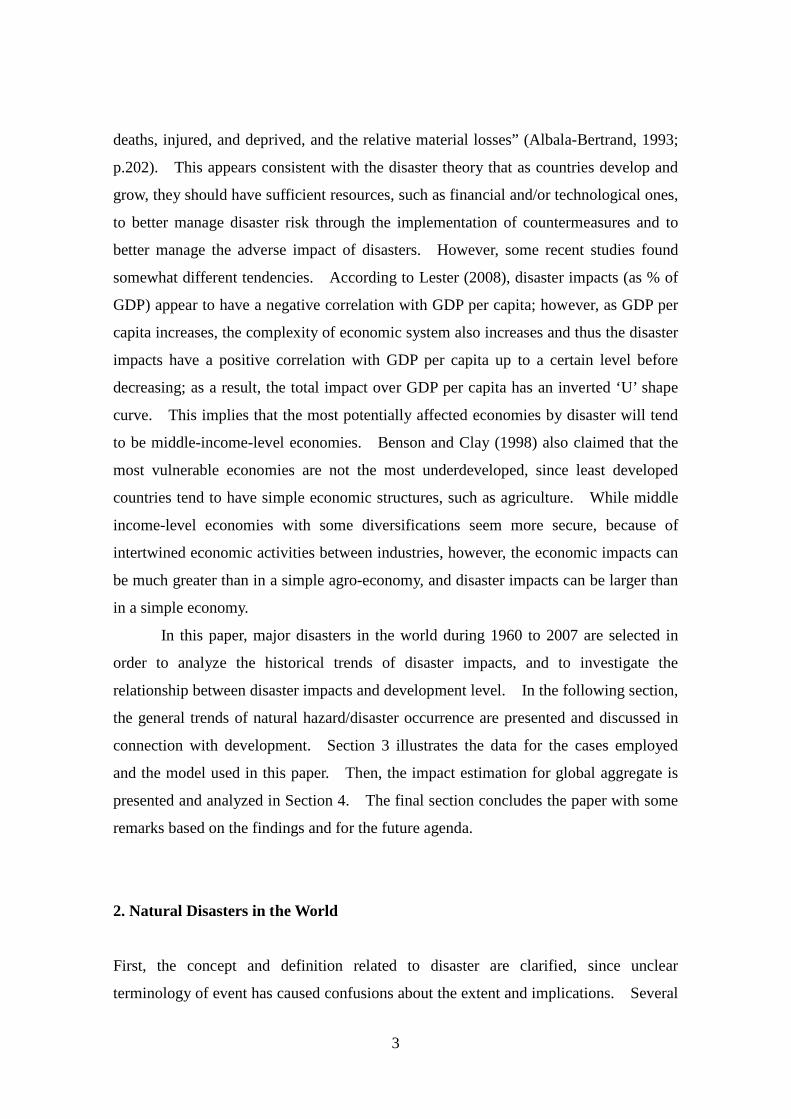
Figure 2-1 indicates the trends of disaster frequency by type between 1900 and 2005.

All types of disaster are increasing, and especially hydro-meteorological ones have

occurred much more frequent than the other two have. On average, 78 disasters per

year had occurred during the 1970s. This number grew to 351 per year during 2000

and 2006. Meanwhile, the average number of people killed in any single disaster has

been declining, making the total number of casualties per year from disasters fairly

constant (UN, 2008).

5

Figure 2-1. Number of Disasters Registered in EMDAT5

5

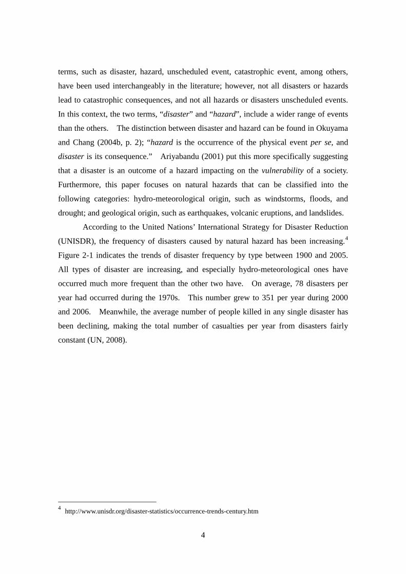
However, economic damages caused by disasters in the world have been also increasing,

especially in the recent years, due partly to more frequent occurrence and also to the

increased complexity of economic structure around the world. Figure 2-2 illustrates

the increasing trends between 1900 and 2008, especially after the mid 1980s, with

several spikes when large-scale disasters occurred. Damages have averaged $83

billion per year since 2000, whereas the average of damages was $12 billion per year

during the 1970s (UN, 2008; constant 2005 US$). These observations lead to the fact

that disasters have become more menacing the well-being of societies, while they have

become less life-threatening.

http://www.unisdr.org/disaster-statistics/occurrence-trends-century.htm; Biological disasters include epidemics and insect infestations.

6

Figure 2-2. Estimated Economic Damage by Disasters Registered in EMDAT6

These observations of the relationship between development level and disaster

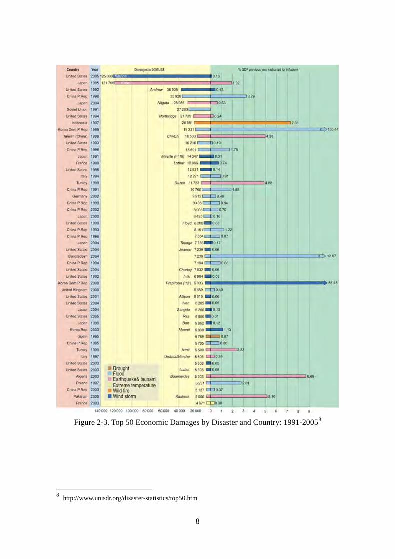
While more than 60% of the total damages caused by disasters occurred in

high-income countries, the estimated damages of disasters as a share of GDP were

significantly greater in less developed (and small) countries (UN, 2008). Figure 2-3

shows the top 50 disasters with largest damages during 1991 and 2005. The largest

damage in this period was the 2005 Hurricane Katrina in the United States, followed by

the 1995 Hanshin-Awaji (Kobe) Earthquake in Japan. While some developing

countries, like China and Indonesia, are included in the top 50 cases, most of the largest

damages occurred in developed countries with relatively small GDP share. In contrast,

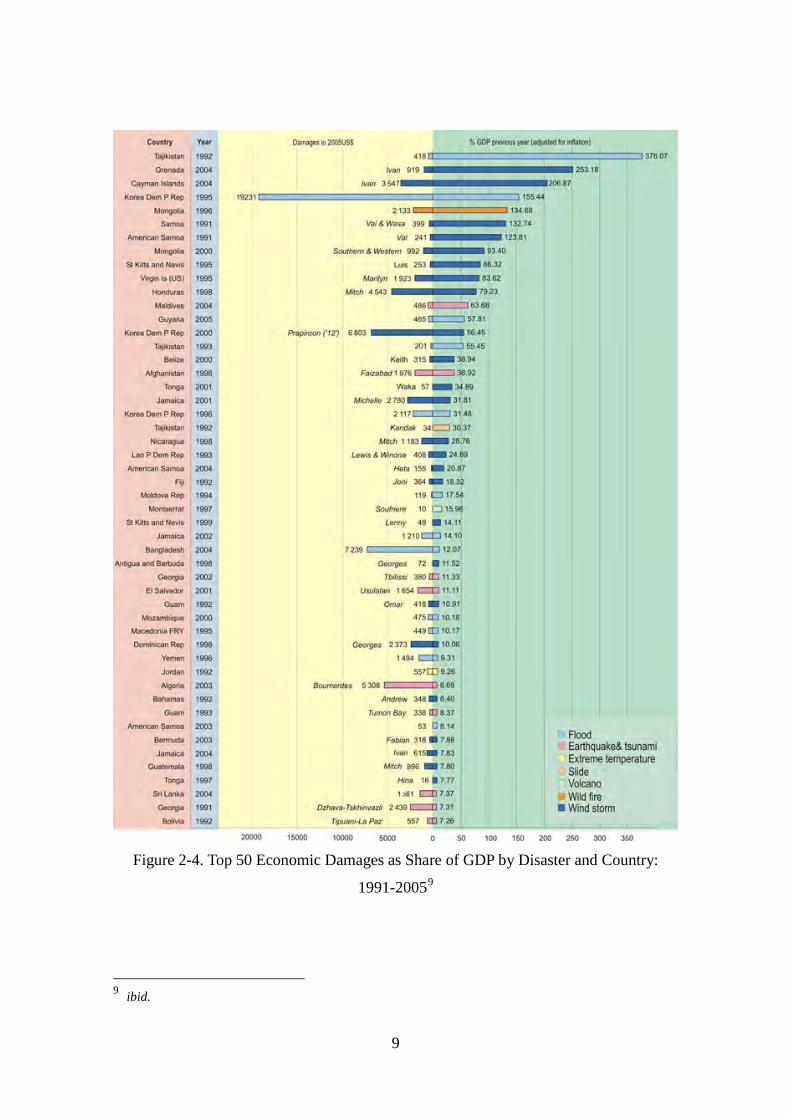
Figure 2-4 presents the top 50 disasters with largest GDP share in the same period. All

the 50 disasters occurred in developing countries, especially in small island countries.

As a matter of fact, no upper middle-income country has been ranked in the top 100 for

most costly disasters as a share of GDP (UN, 2008).

6 http://www.emdat.be/Database/Trends/trends.html

7

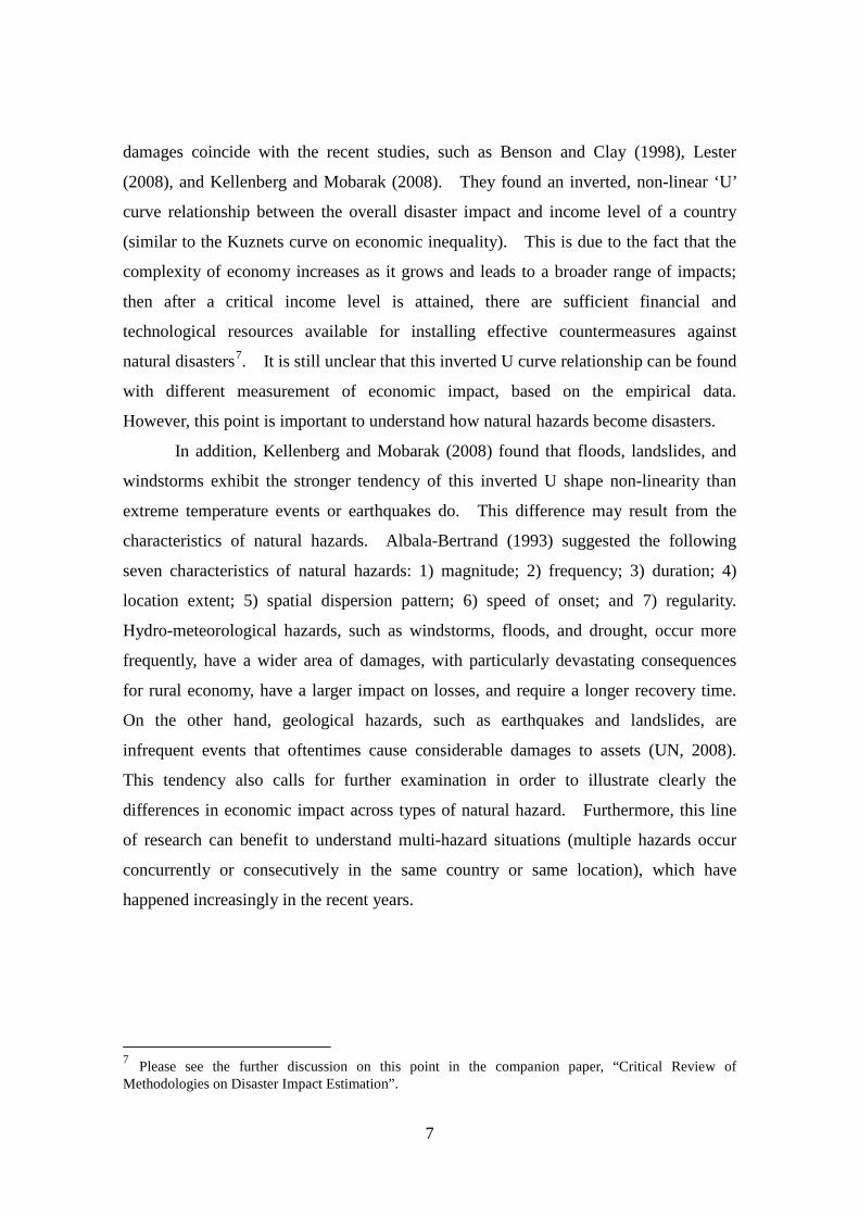
damages coincide with the recent studies, such as Benson and Clay (1998), Lester

(2008), and Kellenberg and Mobarak (2008). They found an inverted, non-linear ‘U’

curve relationship between the overall disaster impact and income level of a country

(similar to the Kuznets curve on economic inequality). This is due to the fact that the

complexity of economy increases as it grows and leads to a broader range of impacts;

then after a critical income level is attained, there are sufficient financial and

technological resources available for installing effective countermeasures against

natural disasters7

7 Please see the further discussion on this point in the companion paper, “Critical Review of Methodologies on Disaster Impact Estimation”.

. It is still unclear that this inverted U curve relationship can be found

with different measurement of economic impact, based on the empirical data.

However, this point is important to understand how natural hazards become disasters.

In addition, Kellenberg and Mobarak (2008) found that floods, landslides, and

windstorms exhibit the stronger tendency of this inverted U shape non-linearity than

extreme temperature events or earthquakes do. This difference may result from the

characteristics of natural hazards. Albala-Bertrand (1993) suggested the following

seven characteristics of natural hazards: 1) magnitude; 2) frequency; 3) duration; 4)

location extent; 5) spatial dispersion pattern; 6) speed of onset; and 7) regularity.

Hydro-meteorological hazards, such as windstorms, floods, and drought, occur more

frequently, have a wider area of damages, with particularly devastating consequences

for rural economy, have a larger impact on losses, and require a longer recovery time.

On the other hand, geological hazards, such as earthquakes and landslides, are

infrequent events that oftentimes cause considerable damages to assets (UN, 2008).

This tendency also calls for further examination in order to illustrate clearly the

differences in economic impact across types of natural hazard. Furthermore, this line

of research can benefit to understand multi-hazard situations (multiple hazards occur

concurrently or consecutively in the same country or same location), which have

happened increasingly in the recent years.

8

Figure 2-3. Top 50 Economic Damages by Disaster and Country: 1991-20058

8 http://www.unisdr.org/disaster-statistics/top50.htm

9

Figure 2-4. Top 50 Economic Damages as Share of GDP by Disaster and Country:

1991-20059

9 ibid.

10

3. Global Aggregation of Disaster Impacts: Data and Methodology

As seen in the previous section, economic damages of disasters have some tendencies

and trends. At the same time, the data for disaster impacts have been still limited and

sometimes confusing due to the use of interchangeable terminologies and to the lack of

standardized definitions. Moreover, while each disaster is unique, economic impacts

of disasters have been analyzed mostly through the case studies of a particular event,

rather than in an aggregated context for the generalized understanding of phenomena.

In this regard, estimating the global aggregate of disaster impacts has been long-sought

in the disaster community. This section presents the data sources for the global

aggregate estimation of disaster impacts in this paper. The data used are mostly

available for public as secondary data, but the definitions and/or extent of disaster

damage data are not standardized to make a direct comparison of the derived impacts

difficult.

3.1. The Case for a Global Aggregate

Natural hazards occur around the world with a wide range of intensities. In order to

set the cases for global aggregate of impact estimation, economic damage, or loss data

of disasters need to be collected. No standardized definitions or frameworks of

economic damage and loss are set so far, except the use of ECLAC methodology (UN

ECLAC, 2003) for recent disasters. Thus, it is difficult to collect the consistent

measurement of economic damage and loss data for past disasters. However, there are

a few sources offer the economic damage or loss data of past disasters: EM-DAT

database by Centre for Research on the Epidemiology of Disasters (CRED) of

Université Catholique de Louvain, NatCat database by Munich Re, and Sigma data base

by Swiss Re.10

The disaster cases are selected from the ones occurred during 1960 to 2007.

As mentioned above, there is no standard definition of economic impact; furthermore,

In this present study, economic damage data are gathered from

EM-DAT and NatCat databases.

10 Some useful comparison of these databases can be found in Guha-Sapir and Below (2002).

11

economic damage, loss, and impact of disasters are used interchangeably in various

documents, including official ones. In fact, EM-DAT uses ‘estimated damage’11

while NatCat’s data is labeled as ‘overall losses’. It is then useful to clarify the

terminology: damages are by economics definition the damages on stocks, which

include physical and human capitals; losses are business interruptions, such as

production and/or consumption, caused by damages and can be considered as first-order

losses; higher-order effects, which take into account the system-wide impact based on

first-order losses through inter-industry relationships; and total impacts are the total of

flow impacts, adding losses (first-order losses) and higher-order effects.12

Then, the disaster cases

Whereas

EM-DAT and NatCat databases used different terms for economic data of disasters, we

consider both of them as damages, i.e. damages on capital stock. 13 are combined between two databases, and are

screened based on the intensity in order to reduce the number of cases by eliminating

smaller cases. The intensity condition is set as: damages should be greater than or

equal to US$ 20 million (current), and either should be greater than 1% of current GDP

for high-income countries or 2% of current GDP for low-income countries. The

number of cases after this screening becomes 184. In order to be used as the input to

estimate total impacts, these damage data were converted first to flow measure, i.e.

losses, using capital-to-output ratio based on the available and estimated capital data14

11 EM-DAT states the definition of estimated damage as: “Several institutions have developed methodologies to quantify these losses in their specific domain. However, there is no standard procedure to determine a global figure for economic impact.” (http://www.emdat.be/ExplanatoryNotes/explanotes.html) 12 Further discussion of terminology can be found in a companion paper, “Critical Review of Methodologies on Disaster Impact Estimation.” 13 These cases include climatological, geophysical, hydrological, and meteorological disasters in EM-DAT definition. 14 Nehru and Dhareshwar (1995), GTAP, and World Bank (2006). Estimation of missing values was carried out using ‘Gross Capital Formation’ data from the World Bank website.

and the current GDP data. The derived losses are further converted to changes in final

demand through dividing losses by the inverse of diagonal terms in the direct input

coefficient matrix. Then, the total impact of each disaster is estimated by plugging this

final demand changes into the respective accounting multiplier matrix, described below.

12

3.2. Economic Impact Estimation Methodology: Social Accounting Matrix

Various methods can be used to estimate higher-order effect of disasters based on

damages and/or losses data, including input-output (IO) table, social accounting matrix

(SAM), and computable general equilibrium (CGE) model.15 Since the cases for

global aggregate include a large group of countries in different years, the data

availability of method becomes one of the key issues for the selection of methodology.

SAM is employed in this study because of its data availability of construction and the

familiarity of use in international development community16

Social accounting matrix (SAM) has been utilized to examine the higher-order

effects across different socio-economic agents, activities, and factors. Notable studies

using a SAM or one of its variants include Cole (1995, 1998, and 2004) among others.

Like IO models, the SAM approach has rigid coefficients and tends to provide upper

bounds of impact estimates. On the other hand, the SAM framework with certain

disaggregation, as well as extended IO model and CGE model, can derive the

distributional impacts of a disaster in order to evaluate equity considerations for public

policies against disasters. In this paper, SAMs were constructed in an aggregated

version for each country and each decade, based on the World Bank data.

.

17

15 A summary and discussion of methodologies on impact estimation can be seen in a companion paper, “Critical Review of Methodologies on Disaster Impact Estimation.” 16 Please see Appendix 1 for detailed description of SAM, and a companion paper, ‘Impact Estimation Methodology: Case Studies.’ 17 SAM structure draws upon the MAMS model (Lofgren and Diaz-Bonilla, 2008), and Lofgren’s SAM template is used to construct SAMs in this exercise (see Hans Lofgren’s course material (2008) on MAMS, for the detail).

Due to the

large number of SAMs that needed to be constructed, and in order to maintain the

consistency of the structure and features among them, the SAMs were constructed in the

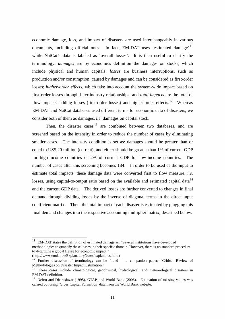
most aggregated way—one sector (one value) for each principal account (see the Figure

3-1). This simple structure is also necessary to suit with the aggregation level of input

data, total damages, for each case.

13

Figure 3-1. Structure of SAM for the Global Aggregate Estimation18

During 1960 to 2007, based on the sampled 184 disasters, total damages on capital

stock were about US$ 742 billion (in 2007 constant value). Estimated losses and total

impacts in this period were US$ 360 billion and US$ 678 billion, respectively. The

impact multiplier from these figures becomes 1.88 (ratio between total impacts and

losses), implying that on average losses from a disaster can be nearly doubled via

4. Analysis of Global Aggregate Disaster Damages, Losses, and Higher-Order

Effects

The economic impact of 184 disasters for the last 50 years are estimated and analyzed in

this section. As described in the previous section, the higher-order effects of these

disasters are derived based on the data from EM-DAT and NatCat and the constructed

SAMs for this study. The historical trends, differences in types of disaster, and the

relationship between disaster impact and development level are investigated below.

4.1. Historical Trends of Impact

18 The highlighted cells are treated as endogenous, and other cells are set as exogenous in this paper.

ProductionActivities Factors Households Other

InstitutionsRest of the

World Total

ProductionActivities

Factors

Households

OtherInstitutions

Rest of theWorld

Total

14

interdependencies in an economy. Table 4-1 shows the distribution of impact across

the types19

19 Climatological disasters include droughts, extreme temperatures, and wildfires; geophysical disasters are earthquakes and volcano eruptions; hydrological disasters are floods and landslides; and meteorological disasters include storms.

of disaster. Over all, geophysical disasters have the largest portion of all

the economic impacts, i.e. damages, losses, and total impacts, with around 40% of the

total impacts. This implies that geophysical disasters cause significant damages on

stock, as well as losses and total impacts. This tendency may result from the fact that

geographical disasters cause the destructions of not only production facilities and

houses but also infrastructure including road networks and lifelines. These damages to

infrastructure propagate economic impacts to a wider extend through economic

interdependencies and may prolong the recovery and reconstruction. Meanwhile,

hydrological and meteorological disasters have the similar shares of economic impacts,

with around 25% of the total. Since these types of disasters have a wider range of

location extent but less destruction of physical assets, the significance of economic

impacts is moderate comparing to geophysical disasters.

15

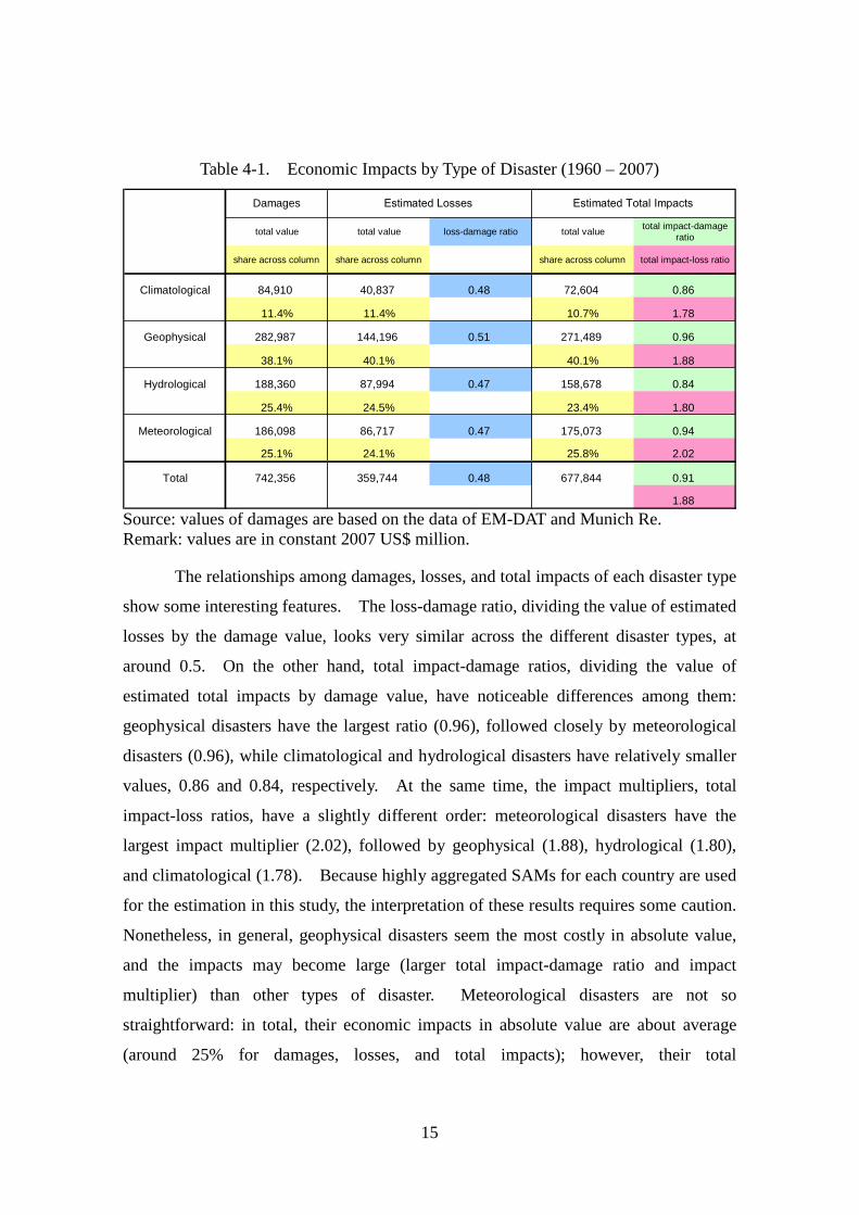
Table 4-1. Economic Impacts by Type of Disaster (1960 – 2007)

Source: values of damages are based on the data of EM-DAT and Munich Re. Remark: values are in constant 2007 US$ million.

The relationships among damages, losses, and total impacts of each disaster type

show some interesting features. The loss-damage ratio, dividing the value of estimated

losses by the damage value, looks very similar across the different disaster types, at

around 0.5. On the other hand, total impact-damage ratios, dividing the value of

estimated total impacts by damage value, have noticeable differences among them:

geophysical disasters have the largest ratio (0.96), followed closely by meteorological

disasters (0.96), while climatological and hydrological disasters have relatively smaller

values, 0.86 and 0.84, respectively. At the same time, the impact multipliers, total

impact-loss ratios, have a slightly different order: meteorological disasters have the

largest impact multiplier (2.02), followed by geophysical (1.88), hydrological (1.80),

and climatological (1.78). Because highly aggregated SAMs for each country are used

for the estimation in this study, the interpretation of these results requires some caution.

Nonetheless, in general, geophysical disasters seem the most costly in absolute value,

and the impacts may become large (larger total impact-damage ratio and impact

multiplier) than other types of disaster. Meteorological disasters are not so

straightforward: in total, their economic impacts in absolute value are about average

(around 25% for damages, losses, and total impacts); however, their total

Damages

total value total value loss-damage ratio total value total impact-damageratio

share across column share across column share across column total impact-loss ratio

Climatological 84,910 40,837 0.48 72,604 0.86

11.4% 11.4% 10.7% 1.78

Geophysical 282,987 144,196 0.51 271,489 0.96

38.1% 40.1% 40.1% 1.88

Hydrological 188,360 87,994 0.47 158,678 0.84

25.4% 24.5% 23.4% 1.80

Meteorological 186,098 86,717 0.47 175,073 0.94

25.1% 24.1% 25.8% 2.02

Total 742,356 359,744 0.48 677,844 0.91

1.88

Estimated Losses Estimated Total Impacts

16

impact-damage ratio and impact multiplier is rather larger, and even the largest. These

imply again that meteorological disasters wipe out a large extent of areas and a large

range of activities resulting in greater total impacts than other types of disasters. In

fact, out of the top ten events with largest impact multipliers, seven events are

meteorological ones (in Madagascar and Guatemala), two are hydrological (in

Madagascar and Bangladesh), and one is geophysical (in Guatemala).

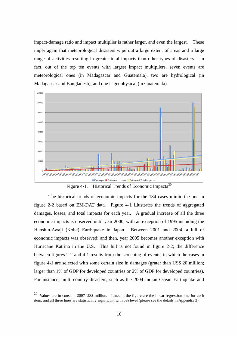
Figure 4-1. Historical Trends of Economic Impacts20

The historical trends of economic impacts for the 184 cases mimic the one in

figure 2-2 based on EM-DAT data. Figure 4-1 illustrates the trends of aggregated

damages, losses, and total impacts for each year. A gradual increase of all the three

economic impacts is observed until year 2000, with an exception of 1995 including the

Hanshin-Awaji (Kobe) Earthquake in Japan. Between 2001 and 2004, a lull of

economic impacts was observed; and then, year 2005 becomes another exception with

Hurricane Katrina in the U.S. This lull is not found in figure 2-2; the difference

between figures 2-2 and 4-1 results from the screening of events, in which the cases in

figure 4-1 are selected with some certain size in damages (grater than US$ 20 million;

larger than 1% of GDP for developed countries or 2% of GDP for developed countries).

For instance, multi-country disasters, such as the 2004 Indian Ocean Earthquake and

20 Values are in constant 2007 US$ million. Lines in the figure are the linear regression line for each item, and all three lines are statistically significant with 5% level (please see the details in Appendix 2).

0

20,000

40,000

60,000

80,000

100,000

120,000

140,000

160,000

1960

1961

1962

1963

1964

1965

1966

1967

1968

1969

1970

1971

1972

1973

1974

1975

1976

1977

1978

1979

1980

1981

1982

1983

1984

1985

1986

1987

1988

1989

1990

1991

1992

1993

1994

1995

1996

1997

1998

1999

2000

2001

2002

2003

2004

2005

2006

2007

Damages Estimated Losses Estimated Total Impacts

17

Tsunami, are separated by affected country and screened; thus, some countries affected

by the events are not included. Therefore, some years in figure 4-1 have much smaller

total damages than in figure 2-2.

The relationships among damages, losses, and total impacts appear different

each year. For example, in 199021, the aggregated total impacts are the largest,

followed by the aggregated losses and the aggregated damages. In 199922

It is a common practice to normalize data in current value with time varying

factors. The analysis above is based on the constant value (in 2007 US$), controlling

inflation over time. In disaster impact analysis, some other factors may need to be

controlled. For instance, Pielke et al. (2008) used the changes in inflation and wealth

at the national level and the changes in population and housing units at coastal county

level for analyzing the trends of hurricane damage in the United States between 1900

, for instance,

the aggregated total impacts are the largest, followed by the aggregated damages and

the aggregated losses. On the other hand, in many years, aggregated damages are the

largest, followed by aggregated total impacts and aggregated losses. Since the

estimation of losses (and of higher-order effects based on losses, and the construction of

SAMs) relies a great deal on capital stock data, which are rarely available and thus are

estimated based mostly on the available data in recent years, and thus the estimated

results are sensitive to capital stock estimation, the above observations of relationship

among these economic impacts cannot be easily generalized. In addition, the

relationship between losses and total impacts needs further attention, because the

damages and/or losses to specific industries can cause different higher-order effects: for

example, damages and/or losses of manufacturing industry may result in a production

bottleneck via forward linkage (supply chain) and backward linkage (demand chain)

and can cause effects in a broader range of industries, depending on how the domestic

(or international) interindustry relationships are intertwined. This kind of

disaggregated analysis of higher-order effects for the recent disasters can be found in a

companion paper, ‘Impact Estimation of Higher-Order Effects: Case Studies’.

21 In 1990, five events are included: floods in Honduras; earthquake in Iran; drought in Mozambique; drought in Namibia; and earthquake in Philippines. 22 Nine events are included in 1999: earthquakes in Columbia, Greece, and Turkey; storms in Denmark and St. Kitts and Nevis; droughts in Iran, Mauritius, and Morocco; and, flood in Venezuela.

18

and 2005. For a cross-country and time-series analysis like this research, it is difficult

to control all the factors; therefore, the Gross World Production (World GDP) is

employed to normalize the disaster impact data by controlling the size of economy in

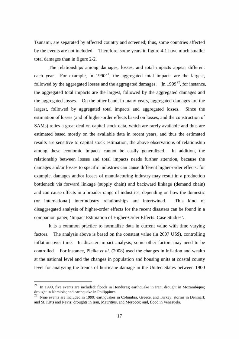
question. Figure 4-2 illustrates the trends of disaster impacts as the share of world

GDP. The trends appear very similar to the ones in absolute value (figure 4-1).

However, the statistical analysis23

Figure 4-2. Historical Trends of Normalized Disaster Impacts

indicates that only the trends of damages and losses

are statistically significant, but being rather weak at 10% level, with a linear trend line

between time and GDP share of total impacts, while the trend of total impacts is not

statistically significant. Not significant trend in total impacts is in fact consistent with

other studies using normalized disaster impact, including abovementioned Pielke et al.

(2008). However, the inconsistency between statistically significant trends of damages

and losses and insignificant total impacts needs to be further investigated, perhaps

including smaller intensity of disasters.

24

The historical trends of normalized economic impacts appear quite different

across the types of disaster (see Figure 4-3). Climatological disasters were increasing

the economic impacts until the early 1980s; and then there was a lull for the remaining

23 Please see the details of statistical analysis with normalized data in Appendix 2. 24 Lines in the figure are the linear regression line for each item, and both lines are statistically significant with 10% level (please see the details in Appendix 2).

0.00%

0.05%

0.10%

0.15%

0.20%

0.25%

0.30%

0.35%

0.40%

1960

1962

1964

1966

1968

1970

1972

1974

1976

1978

1980

1982

1984

1986

1988

1990

1992

1994

1996

1998

2000

2002

2004

2006

Damages Estimated Losses Estimated Total Impacts

19

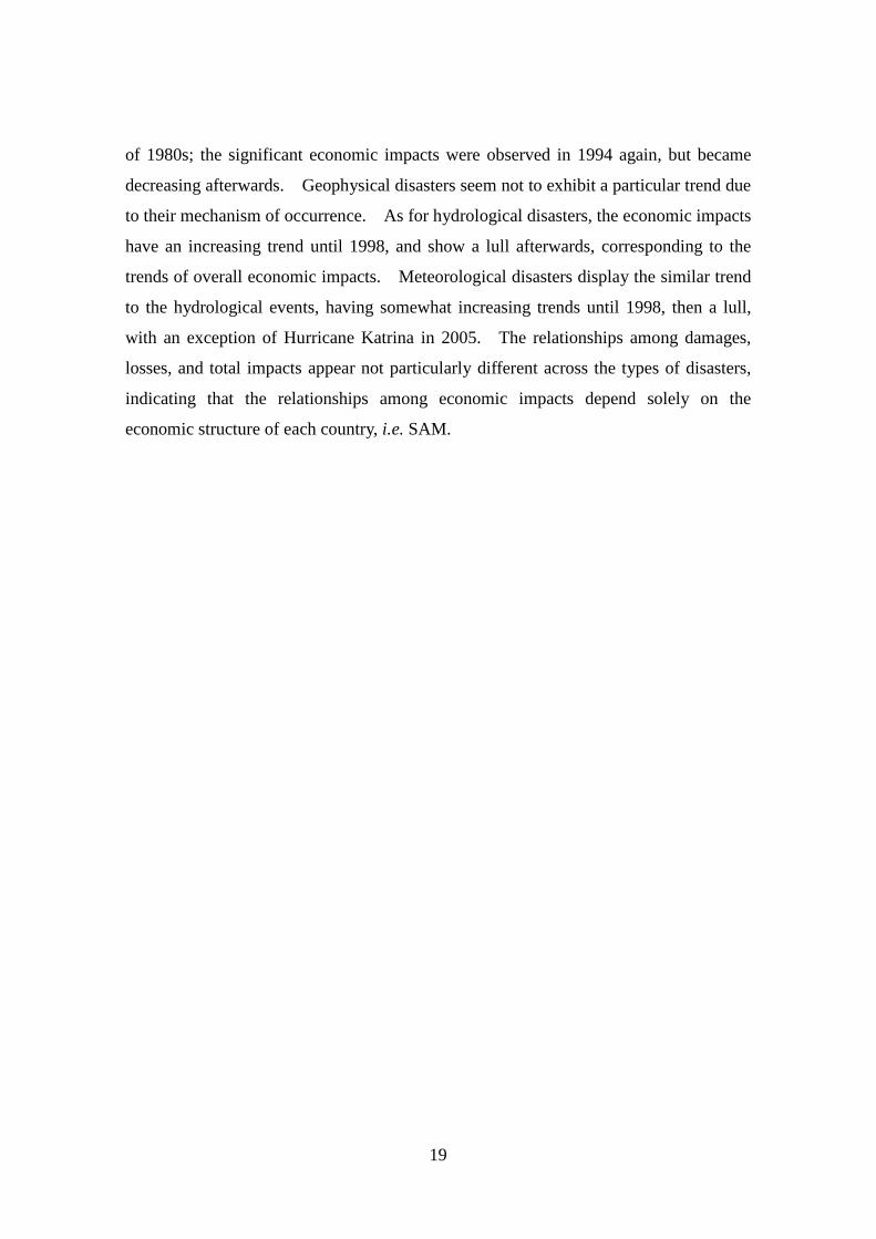
of 1980s; the significant economic impacts were observed in 1994 again, but became

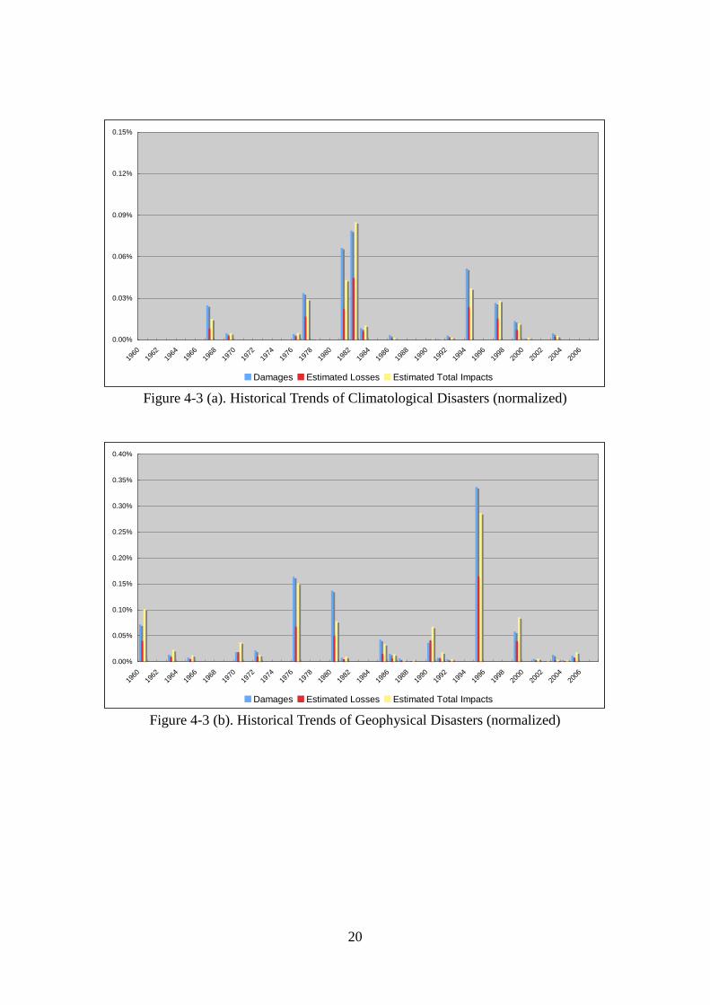
decreasing afterwards. Geophysical disasters seem not to exhibit a particular trend due

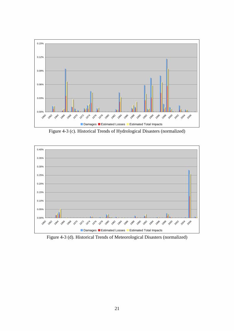
to their mechanism of occurrence. As for hydrological disasters, the economic impacts

have an increasing trend until 1998, and show a lull afterwards, corresponding to the

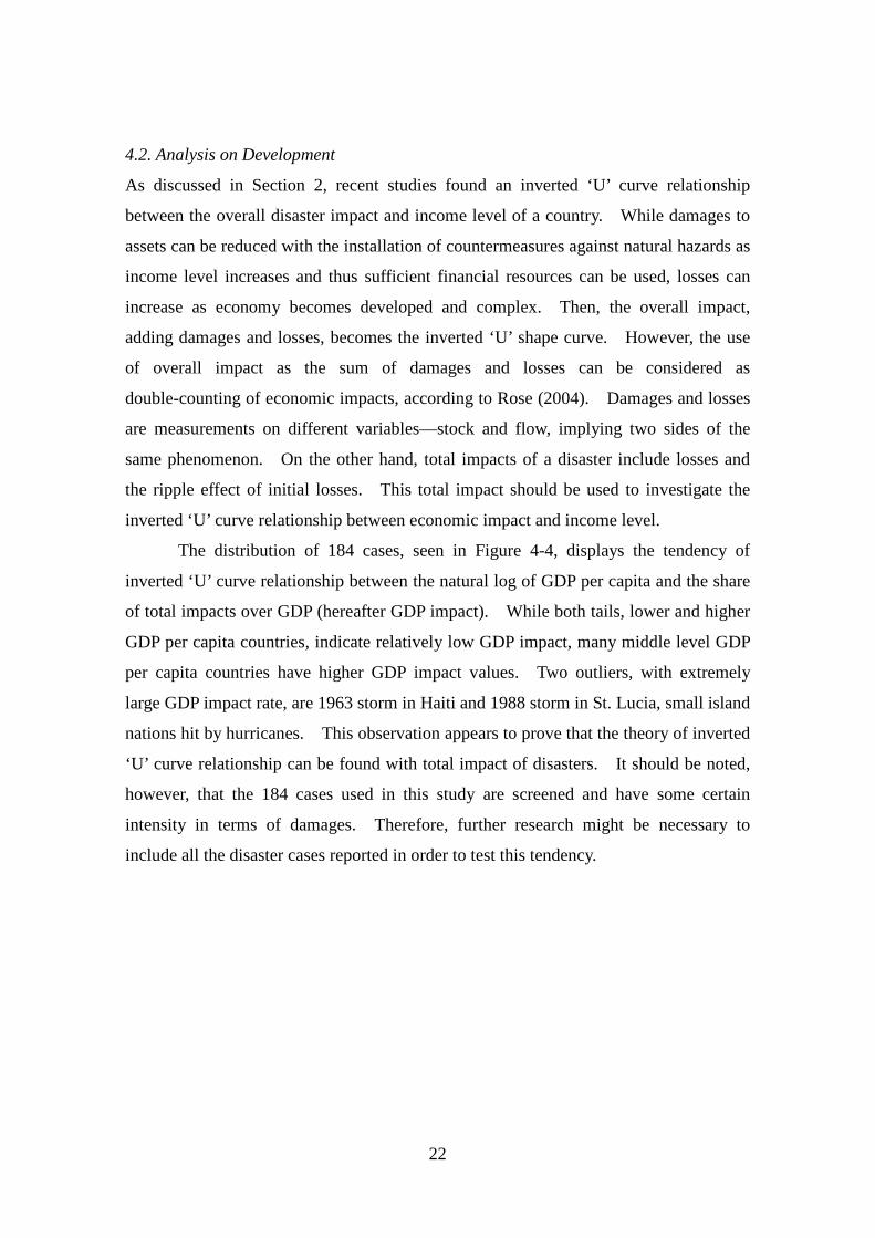
trends of overall economic impacts. Meteorological disasters display the similar trend

to the hydrological events, having somewhat increasing trends until 1998, then a lull,

with an exception of Hurricane Katrina in 2005. The relationships among damages,

losses, and total impacts appear not particularly different across the types of disasters,

indicating that the relationships among economic impacts depend solely on the

economic structure of each country, i.e. SAM.

20

Figure 4-3 (a). Historical Trends of Climatological Disasters (normalized)

Figure 4-3 (b). Historical Trends of Geophysical Disasters (normalized)

0.00%

0.03%

0.06%

0.09%

0.12%

0.15%

1960

1962

1964

1966

1968

1970

1972

1974

1976

1978

1980

1982

1984

1986

1988

1990

1992

1994

1996

1998

2000

2002

2004

2006

Damages Estimated Losses Estimated Total Impacts

0.00%

0.05%

0.10%

0.15%

0.20%

0.25%

0.30%

0.35%

0.40%

1960

1962

1964

1966

1968

1970

1972

1974

1976

1978

1980

1982

1984

1986

1988

1990

1992

1994

1996

1998

2000

2002

2004

2006

Damages Estimated Losses Estimated Total Impacts

21

Figure 4-3 (c). Historical Trends of Hydrological Disasters (normalized)

Figure 4-3 (d). Historical Trends of Meteorological Disasters (normalized)

0.00%

0.03%

0.06%

0.09%

0.12%

0.15%

1960

1962

1964

1966

1968

1970

1972

1974

1976

1978

1980

1982

1984

1986

1988

1990

1992

1994

1996

1998

2000

2002

2004

2006

Damages Estimated Losses Estimated Total Impacts

0.00%

0.05%

0.10%

0.15%

0.20%

0.25%

0.30%

0.35%

0.40%

1960

1962

1964

1966

1968

1970

1972

1974

1976

1978

1980

1982

1984

1986

1988

1990

1992

1994

1996

1998

2000

2002

2004

2006

Damages Estimated Losses Estimated Total Impacts

22

4.2. Analysis on Development

As discussed in Section 2, recent studies found an inverted ‘U’ curve relationship

between the overall disaster impact and income level of a country. While damages to

assets can be reduced with the installation of countermeasures against natural hazards as

income level increases and thus sufficient financial resources can be used, losses can

increase as economy becomes developed and complex. Then, the overall impact,

adding damages and losses, becomes the inverted ‘U’ shape curve. However, the use

of overall impact as the sum of damages and losses can be considered as

double-counting of economic impacts, according to Rose (2004). Damages and losses

are measurements on different variables—stock and flow, implying two sides of the

same phenomenon. On the other hand, total impacts of a disaster include losses and

the ripple effect of initial losses. This total impact should be used to investigate the

inverted ‘U’ curve relationship between economic impact and income level.

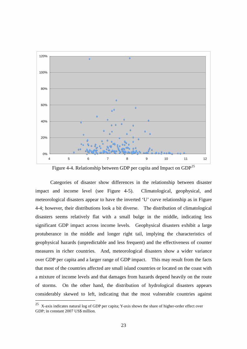
The distribution of 184 cases, seen in Figure 4-4, displays the tendency of

inverted ‘U’ curve relationship between the natural log of GDP per capita and the share

of total impacts over GDP (hereafter GDP impact). While both tails, lower and higher

GDP per capita countries, indicate relatively low GDP impact, many middle level GDP

per capita countries have higher GDP impact values. Two outliers, with extremely

large GDP impact rate, are 1963 storm in Haiti and 1988 storm in St. Lucia, small island

nations hit by hurricanes. This observation appears to prove that the theory of inverted

‘U’ curve relationship can be found with total impact of disasters. It should be noted,

however, that the 184 cases used in this study are screened and have some certain

intensity in terms of damages. Therefore, further research might be necessary to

include all the disaster cases reported in order to test this tendency.

23

Figure 4-4. Relationship between GDP per capita and Impact on GDP25

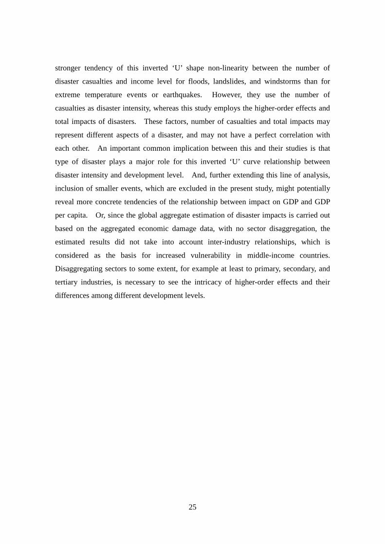
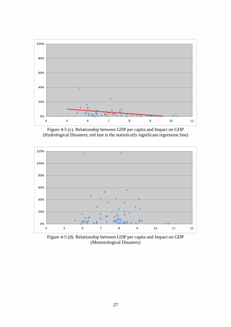
Categories of disaster show differences in the relationship between disaster

impact and income level (see Figure 4-5). Climatological, geophysical, and

meteorological disasters appear to have the inverted ‘U’ curve relationship as in Figure

4-4; however, their distributions look a bit diverse. The distribution of climatological

disasters seems relatively flat with a small bulge in the middle, indicating less

significant GDP impact across income levels. Geophysical disasters exhibit a large

protuberance in the middle and longer right tail, implying the characteristics of

geophysical hazards (unpredictable and less frequent) and the effectiveness of counter

measures in richer countries. And, meteorological disasters show a wider variance

over GDP per capita and a larger range of GDP impact. This may result from the facts

that most of the countries affected are small island countries or located on the coast with

a mixture of income levels and that damages from hazards depend heavily on the route

of storms. On the other hand, the distribution of hydrological disasters appears

considerably skewed to left, indicating that the most vulnerable countries against

25 X-axis indicates natural log of GDP per capita; Y-axis shows the share of higher-order effect over GDP; in constant 2007 US$ million.

0%

20%

40%

60%

80%

100%

120%

4 5 6 7 8 9 10 11 12

24

hydrological disasters are low-income countries. This is because hydrological

disasters, such as floods and landslides, “have a wider impact, with particularly

devastating consequences for rural economy (p. 80)” (UN, 2008). Those countries

having lowest income countries with higher GDP impact are Bangladesh, Mozambique,

and Nepal.

A series of statistical analyses is performed to see whether or not the inverted U

curve relationship actually exists for the above cases26

These results, to some extent, may contradict with Kellenberg and Mobarak’s

(2008) study, in which with the data of 133 countries over 28 years they found the

. The results show that inverted

U curve relationship (non-linear function form) in either all events case or any type of

disasters is not statistically significant, contrary to the above visual inspections. On

the other hand, negative linear relationships are statistically significant with

climatological, geophysical, and hydrological events. For the cases with all the 184

events and with meteorological events, neither linear nor non-linear form is statistically

significant. The negative linear relationship is, in fact, consistent with the traditional

disaster theory, in which as development level, i.e. income level, increases, the risk for

disaster impacts decreases. A striking finding of the statistical analysis is that the

slope of the statistically significant regression line is much steeper in geophysical

disasters than in the other two cases (climatological and hydrological): around two

times steeper. This also signifies the characteristics of disaster. Geophysical

disasters damage mostly the structure of built environment; therefore, as national

income rises, the better structure of buildings and housing can become affordable and

utilized and the total impacts may become relatively small, and the efficacy of such

solid structure appear effective to reduce the impacts of geophysical disasters. On the

other hand, climatic and hydrological disasters may damage the functions of society and

economy in a wide area; thus, national income increase might not have such a direct

improvement. In addition, while statistically insignificant, the results of non-linear

form display some interesting findings. Among four types of disasters, climatological,

geophysical, and meteorological events indicate an inverted U curve relationship, while

hydrological events show a U curve relationship.

26 Please see Appendix 3 for detailed results and discussions.

25

stronger tendency of this inverted ‘U’ shape non-linearity between the number of

disaster casualties and income level for floods, landslides, and windstorms than for

extreme temperature events or earthquakes. However, they use the number of

casualties as disaster intensity, whereas this study employs the higher-order effects and

total impacts of disasters. These factors, number of casualties and total impacts may

represent different aspects of a disaster, and may not have a perfect correlation with

each other. An important common implication between this and their studies is that

type of disaster plays a major role for this inverted ‘U’ curve relationship between

disaster intensity and development level. And, further extending this line of analysis,

inclusion of smaller events, which are excluded in the present study, might potentially

reveal more concrete tendencies of the relationship between impact on GDP and GDP

per capita. Or, since the global aggregate estimation of disaster impacts is carried out

based on the aggregated economic damage data, with no sector disaggregation, the

estimated results did not take into account inter-industry relationships, which is

considered as the basis for increased vulnerability in middle-income countries.

Disaggregating sectors to some extent, for example at least to primary, secondary, and

tertiary industries, is necessary to see the intricacy of higher-order effects and their

differences among different development levels.

26

Figure 4-5 (a). Relationship between GDP per capita and Impact on GDP (Climatological Disasters; red line is the statistically significant regression line)

Figure 4-5 (b). Relationship between GDP per capita and Impact on GDP (Geophysical Disasters; red line is the statistically significant regression line)

0%

20%

40%

60%

80%

100%

4 5 6 7 8 9 10 11

0%

20%

40%

60%

80%

100%

4 5 6 7 8 9 10 11 12

27

Figure 4-5 (c). Relationship between GDP per capita and Impact on GDP (Hydrological Disasters; red line is the statistically significant regression line)

Figure 4-5 (d). Relationship between GDP per capita and Impact on GDP (Meteorological Disasters)

0%

20%

40%

60%

80%

100%

4 5 6 7 8 9 10 11

0%

20%

40%

60%

80%

100%

120%

4 5 6 7 8 9 10 11 12

28

5. Summary and Conclusions

This paper estimated the global aggregate of the economic impact of major disasters

during 1960 to 2007 using SAM methodology and examined the trends of estimated

disaster impact. The results indicate, in total, the global aggregate of damages is about

US$742 billion, losses are US$360 billion, and total impacts are estimated close to

US$680 billion, in 2007 value. While geophysical disasters are most costly in terms of

absolute value for damages, losses, and total impacts, meteorological disasters have the

highest impact multiplier of 2.02, indicating that damages and losses can spread to a

wider extent through interdependency of economic activities. Moreover, the analysis

indicates a growing trend of economic impacts, such as damages, losses, and total

impacts, over time using all the 184 events, whereas the trends of damages and losses

are statistically significant with linear regression lines. The impact multiplier of the

globally aggregated results over the period becomes nearly two, implying that on

average the losses caused by a disaster can become doubled through the

interdependencies of an economy. Furthermore, the investigation of economic impacts

and development level was carried out to see whether or not an inverted ‘U’ curve

relationship between total impacts and income level can be observed. The statistical

analyses, however, found that inverted U curve relationship, or more generally quadratic

relationship, is not statistically significant for total and each type, while climatological,

geophysical, and hydrological disasters show a negative linear relationship, confirming

the traditional disaster theory, indicating lower-income countries are more vulnerable to

higher-order effects than in middle- or higher- income countries. These results conflict

with Kellenberg and Mobarak’s (2008) study, in which they use the number of

casualties as the disaster impact.

The results in this paper were derived from the damage data of EM-DAT and

NatCat database and using SAM for each country in each decade. These damage data

and SAMs are highly aggregated without having any sector-level information. For an

analysis of historical trends and for international comparison, the aggregation level in

this study is acceptable due to the data availability. On the other hand, further detailed

analysis, based on disaggregated sectors and/or space, can reveal a more thorough and

comprehensive figure of disaster impacts, as presented in a companion paper ‘Impact

29

Estimation Methodology: Case Studies.’ While more sophisticated analysis requires

further precise numerical input data (West and Lenze, 1994), some standardized

framework, such as the ECLAC methodology (UN ECLAC, 2003), can guide us on

how to gather the more detailed data in a consistent way for future disasters. And, if

some common economic model of nations, such as SAM with some level of

disaggregation, becomes available, the estimation and examination of disaster impacts

will provide not only a clearer and more complete picture, but also a broader and more

robust picture of what happens during a disaster. In this regard, the role of

international organizations is particularly important.

30

References

Albala-Bertrand, J.M. (1993) The Political Economy of Large Natural Disasters: With Special Reference to Developing Countries (Oxford, UK: Clarendon Press).

Ariyabandu, M.M. (2001) Bringing together disaster and development - concepts and practice, some experience from South Asia, Paper presented at the 5th European Sociological Association Conference, in Helsinki, August 28th-September 1st, 2001.

Benson, C. and Clay, E. (1998) The impact of drought on sub-Saharan African economies, Technical paper 401, Washington DC: World Bank.

Cole, S. (1995) Lifeline and livelihood: a social accounting matrix approach to calamity preparedness, Journal of Contingencies and Crisis Management, 3, pp. 228-40.

Cole, S. (1998) Decision support for calamity preparedness: socioeconomic and interregional impacts, in: M. Shinozuka, A. Rose and R.T. Eguchi (Eds) Engineering and Socioeconomic Impacts of Earthquakes, pp. 125-153 (Buffalo, NY: Multidisciplinary Center for Earthquake Engineering Research).

Cole, S. (2004) Geohazards in social systems: an insurance matrix approach, in: Y. Okuyama and S.E. Chang (Eds) Modeling Spatial and Economic Impacts of Disasters, pp. 103-118 (New York: Springer).

Davis, D.R. and Weinstein, D.E. (2004) A search for multiple equilibria in urban industrial structure, Working Paper 10252, National Bureau of Economic Research.

Guha-Sapir, D. and R. Below (2002) The Quality and Accuracy of Disaster Data: a Comparative Analysis of Three Global Data Sets. A report for the ProVention Consortium, the Disaster Management Facility, the World Bank.

Kellenberg, D.K. and A.M. Mobarak. (2008) Does rising income increase or decrease damage risk from natural disasters? Journal of Urban Economics, 63: 788-802.

Lester, R. (2008) Climate change, development and the insurance sector”, Policy Research Working Paper, World Bank.

Lofgren, H. (2008) Course material “Introduction to Fiscal Policy with MAMS”, Poverty Reduction and Economic Management Network Economic Policy and Dept, March 13, 2008, at The World Bank, Washington D.C.

Lofgren, H. and C. Diaz-Bonilla (2008) “MAMS: An Economy-wide Model for Analysis of MDG Country Strategies – an application to Latin America and the Caribbean”, mimeo, Development Economics Prospects Group, The World Bank.

Nehru, V. and A. Dhareshwar (1995) Physical Capital Stock: Sources, Methodology and Results Dataset, http://econ.worldbank.org/WBSITE/EXTERNAL/EXTDEC/EXTRESEARCH/0,,contentMDK:20699834~pagePK:64214825~piPK:64214943~theSitePK:469382,00.html, accessed on September 26, 2008.

Pielke, R.A., Jr., Gratz, J., Landsea, C.W., Collins, D., Saunders, M.A., and Musulin, R.

31

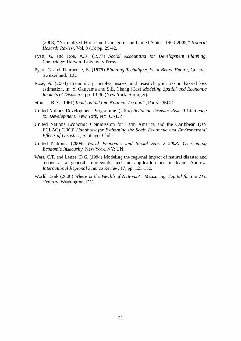
(2008) “Normalized Hurricane Damage in the United States: 1900-2005,” Natural Hazards Review, Vol. 9 (1): pp. 29-42.

Pyatt, G. and Roe, A.R. (1977) Social Accounting for Development Planning, Cambridge: Harvard University Press.

Pyatt, G. and Thorbecke, E. (1976) Planning Techniques for a Better Future, Geneve, Switzerland: ILO.

Rose, A. (2004) Economic principles, issues, and research priorities in hazard loss estimation, in: Y. Okuyama and S.E. Chang (Eds) Modeling Spatial and Economic Impacts of Disasters, pp. 13-36 (New York: Springer).

Stone, J.R.N. (1961) Input-output and National Accounts, Paris: OECD.

United Nations Development Programme. (2004) Reducing Disaster Risk: A Challenge for Development. New York, NY: UNDP.

United Nations Economic Commission for Latin America and the Caribbean (UN ECLAC) (2003) Handbook for Estimating the Socio-Economic and Environmental Effects of Disasters, Santiago, Chile.

United Nations. (2008) World Economic and Social Survey 2008: Overcoming Economic Insecurity. New York, NY: UN.

West, C.T. and Lenze, D.G. (1994) Modeling the regional impact of natural disaster and recovery: a general framework and an application to hurricane Andrew, International Regional Science Review, 17, pp. 121-150.

World Bank (2006) Where is the Wealth of Nations? : Measuring Capital for the 21st Century. Washington, DC.

32

Appendices

Appendix 1. Description of Social Accounting Matrix

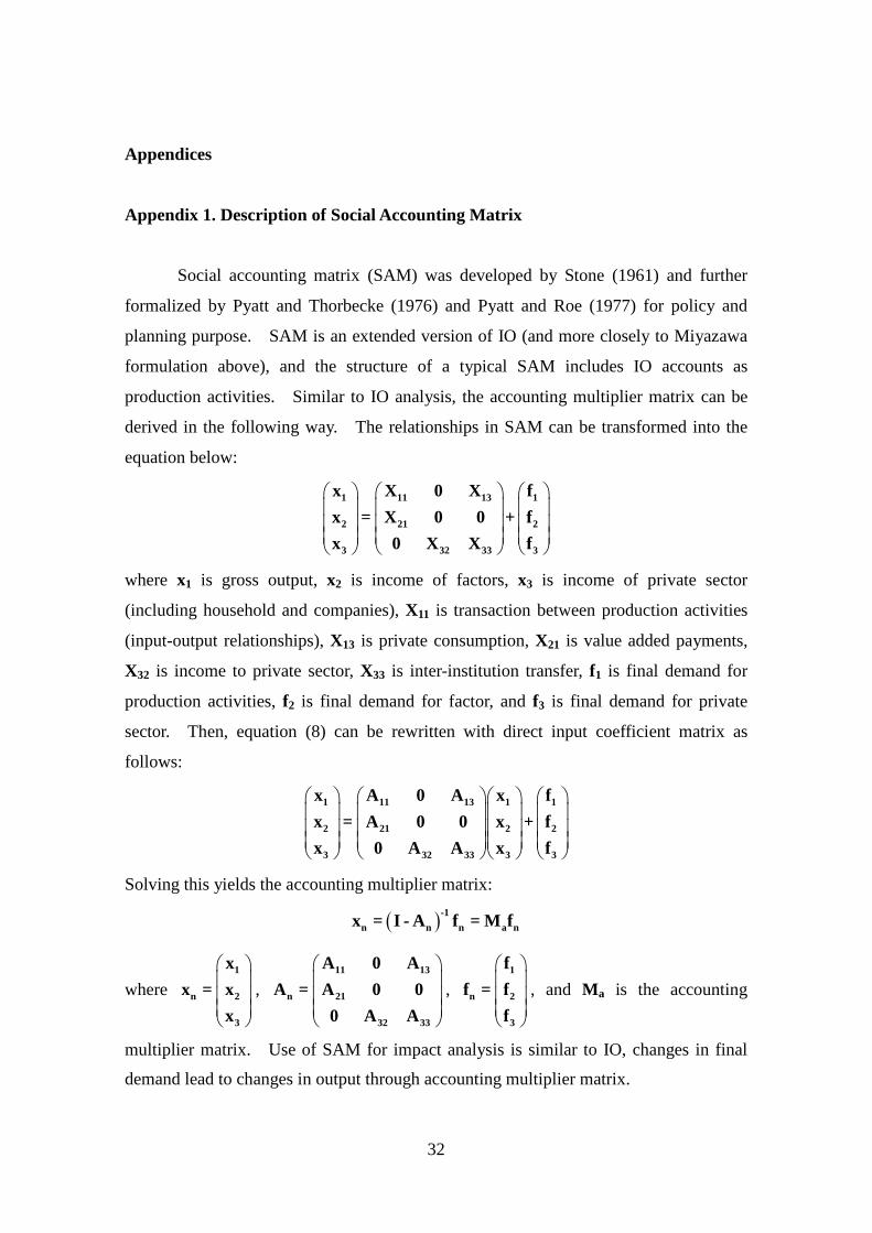
Social accounting matrix (SAM) was developed by Stone (1961) and further

formalized by Pyatt and Thorbecke (1976) and Pyatt and Roe (1977) for policy and

planning purpose. SAM is an extended version of IO (and more closely to Miyazawa

formulation above), and the structure of a typical SAM includes IO accounts as

production activities. Similar to IO analysis, the accounting multiplier matrix can be

derived in the following way. The relationships in SAM can be transformed into the

equation below:

1 11 13 1

2 21 2

3 32 33 3

x X 0 X fx = X 0 0 + fx 0 X X f

where x1 is gross output, x2 is income of factors, x3 is income of private sector

(including household and companies), X11 is transaction between production activities

(input-output relationships), X13 is private consumption, X21 is value added payments,

X32 is income to private sector, X33 is inter-institution transfer, f1 is final demand for

production activities, f2 is final demand for factor, and f3 is final demand for private

sector. Then, equation (8) can be rewritten with direct input coefficient matrix as

follows:

1 11 13 1 1

2 21 2 2

3 32 33 3 3

x A 0 A x fx = A 0 0 x + fx 0 A A x f

Solving this yields the accounting multiplier matrix:

( )-1n n n a nx = I - A f = M f

where

1

n 2

3

xx = x

x,

11 13

n 21

32 33

A 0 AA = A 0 0

0 A A,

1

n 2

3

ff = f

f, and Ma is the accounting

multiplier matrix. Use of SAM for impact analysis is similar to IO, changes in final

demand lead to changes in output through accounting multiplier matrix.

33

Appendix 2. Statistical Analysis of Disaster Impact Trends

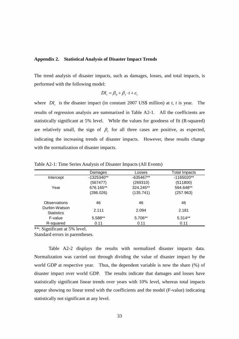
The trend analysis of disaster impacts, such as damages, losses, and total impacts, is

performed with the following model:

0 1t tDI tβ β ε= + ⋅ +

where tDI is the disaster impact (in constant 2007 US$ million) at t, t is year. The

results of regression analysis are summarized in Table A2-1. All the coefficients are

statistically significant at 5% level. While the values for goodness of fit (R-squared)

are relatively small, the sign of 1β for all three cases are positive, as expected,

indicating the increasing trends of disaster impacts. However, these results change

with the normalization of disaster impacts.

Table A2-1: Time Series Analysis of Disaster Impacts (All Events)

**: Significant at 5% level. Standard errors in parentheses.

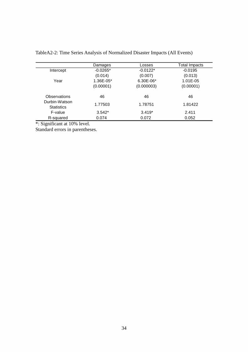
Table A2-2 displays the results with normalized disaster impacts data.

Normalization was carried out through dividing the value of disaster impact by the

world GDP at respective year. Thus, the dependent variable is now the share (%) of

disaster impact over world GDP. The results indicate that damages and losses have

statistically significant linear trends over years with 10% level, whereas total impacts

appear showing no linear trend with the coefficients and the model (F-value) indicating

statistically not significant at any level.

Damages Losses Total ImpactsIntercept -1325340** -635467** -1165020**

(567477) (269310) (511800)Year 676.165** 324.245** 594.648**

(286.026) (135.741) (257.963)

Observations 46 46 46Durbin-Watson

Statistics 2.111 2.094 2.181

F-value 5.588** 5.706** 5.314**R-squared 0.11 0.11 0.11

34

TableA2-2: Time Series Analysis of Normalized Disaster Impacts (All Events)

*: Significant at 10% level. Standard errors in parentheses.

Damages Losses Total ImpactsIntercept -0.0265* -0.0122* -0.0195

(0.014) (0.007) (0.013)Year 1.36E-05* 6.30E-06* 1.01E-05

(0.00001) (0.000003) (0.00001)

Observations 46 46 46Durbin-Watson

Statistics 1.77503 1.78751 1.81422

F-value 3.542* 3.419* 2.411R-squared 0.074 0.072 0.052

35

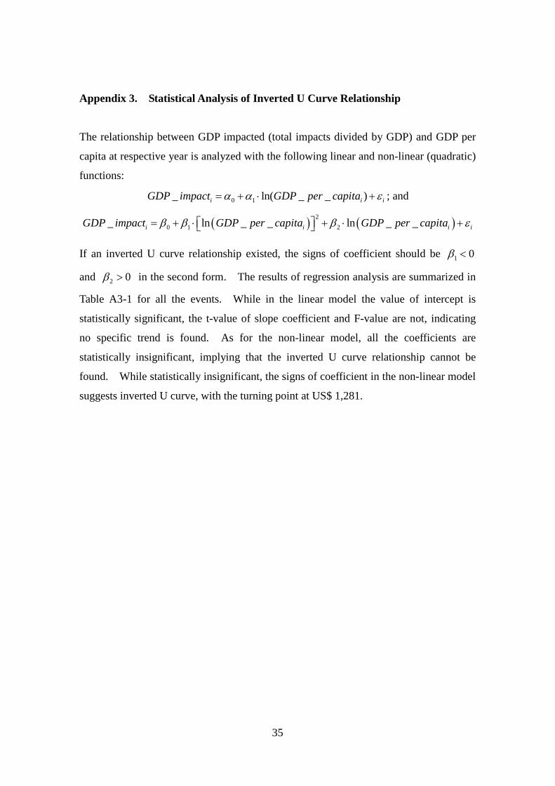
Appendix 3. Statistical Analysis of Inverted U Curve Relationship

The relationship between GDP impacted (total impacts divided by GDP) and GDP per

capita at respective year is analyzed with the following linear and non-linear (quadratic)

functions:

0 1_ ln( _ _ )i i iGDP impact GDP per capitaα α ε= + ⋅ + ; and

( ) ( )20 1 2_ ln _ _ ln _ _i i i iGDP impact GDP per capita GDP per capitaβ β β ε= + ⋅ + ⋅ +

If an inverted U curve relationship existed, the signs of coefficient should be 1 0β <

and 2 0β > in the second form. The results of regression analysis are summarized in

Table A3-1 for all the events. While in the linear model the value of intercept is

statistically significant, the t-value of slope coefficient and F-value are not, indicating

no specific trend is found. As for the non-linear model, all the coefficients are

statistically insignificant, implying that the inverted U curve relationship cannot be

found. While statistically insignificant, the signs of coefficient in the non-linear model

suggests inverted U curve, with the turning point at US$ 1,281.

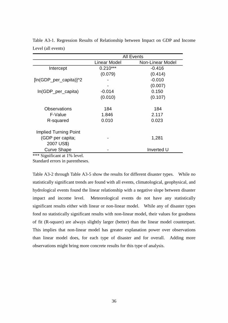
36

Table A3-1. Regression Results of Relationship between Impact on GDP and Income

Level (all events)

*** Significant at 1% level. Standard errors in parentheses.

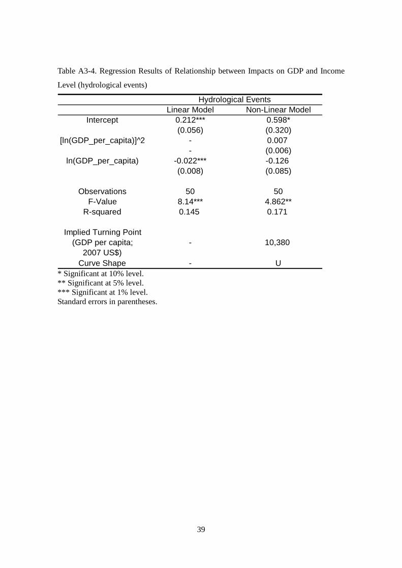
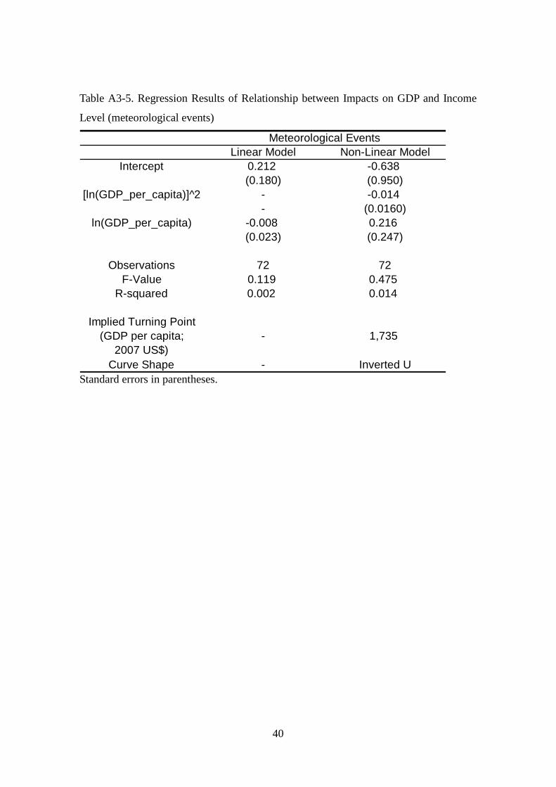
Table A3-2 through Table A3-5 show the results for different disaster types. While no

statistically significant trends are found with all events, climatological, geophysical, and

hydrological events found the linear relationship with a negative slope between disaster

impact and income level. Meteorological events do not have any statistically

significant results either with linear or non-linear model. While any of disaster types

fond no statistically significant results with non-linear model, their values for goodness

of fit (R-square) are always slightly larger (better) than the linear model counterpart.

This implies that non-linear model has greater explanation power over observations

than linear model does, for each type of disaster and for overall. Adding more

observations might bring more concrete results for this type of analysis.

Linear Model Non-Linear ModelIntercept 0.210*** -0.416

(0.079) (0.414)[ln(GDP_per_capita)]^2 - -0.010

- (0.007)ln(GDP_per_capita) -0.014 0.150

(0.010) (0.107)

Observations 184 184F-Value 1.846 2.117

R-squared 0.010 0.023

Implied Turning Point(GDP per capita;

2007 US$)- 1,281

Curve Shape - Inverted U

All Events

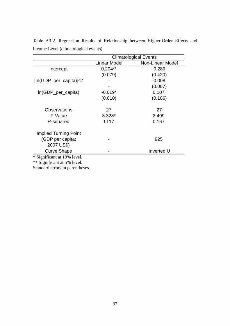
37

Table A3-2. Regression Results of Relationship between Higher-Order Effects and

Income Level (climatological events)

* Significant at 10% level. ** Significant at 5% level. Standard errors in parentheses.

Linear Model Non-Linear ModelIntercept 0.204** -0.289

(0.079) (0.420)[ln(GDP_per_capita)]^2 - -0.008

- (0.007)ln(GDP_per_capita) -0.019* 0.107

(0.010) (0.106)

Observations 27 27F-Value 3.328* 2.409

R-squared 0.117 0.167

Implied Turning Point(GDP per capita;

2007 US$)- 925

Curve Shape - Inverted U

Climatological Events

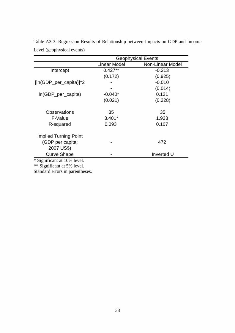
38

Table A3-3. Regression Results of Relationship between Impacts on GDP and Income

Level (geophysical events)

* Significant at 10% level. ** Significant at 5% level. Standard errors in parentheses.

Linear Model Non-Linear ModelIntercept 0.427** -0.213

(0.172) (0.925)[ln(GDP_per_capita)]^2 - -0.010

- (0.014)ln(GDP_per_capita) -0.040* 0.121

(0.021) (0.228)

Observations 35 35F-Value 3.401* 1.923

R-squared 0.093 0.107

Implied Turning Point(GDP per capita;

2007 US$)- 472

Curve Shape - Inverted U

Geophysical Events

39

Table A3-4. Regression Results of Relationship between Impacts on GDP and Income

Level (hydrological events)

* Significant at 10% level. ** Significant at 5% level. *** Significant at 1% level. Standard errors in parentheses.

Linear Model Non-Linear ModelIntercept 0.212*** 0.598*

(0.056) (0.320)[ln(GDP_per_capita)]^2 - 0.007

- (0.006)ln(GDP_per_capita) -0.022*** -0.126

(0.008) (0.085)

Observations 50 50F-Value 8.14*** 4.862**

R-squared 0.145 0.171

Implied Turning Point(GDP per capita;

2007 US$)- 10,380

Curve Shape - U

Hydrological Events

40

Table A3-5. Regression Results of Relationship between Impacts on GDP and Income

Level (meteorological events)

Standard errors in parentheses.

Linear Model Non-Linear ModelIntercept 0.212 -0.638

(0.180) (0.950)[ln(GDP_per_capita)]^2 - -0.014

- (0.0160)ln(GDP_per_capita) -0.008 0.216

(0.023) (0.247)

Observations 72 72F-Value 0.119 0.475

R-squared 0.002 0.014

Implied Turning Point(GDP per capita;

2007 US$)- 1,735

Curve Shape - Inverted U

Meteorological Events