IMF Country Report No. 13/199 CHILE · IMF Country Report No. 13/199 CHILE Selected Issues ......

©2013 International Monetary Fund

IMF Country Report No. 13/199

CHILE

Selected Issues This Selected Issues Paper for Chile was prepared by a staff team of the International Monetary Fund as background documentation for the periodic consultation with the member country. It is based on the information available at the time it was completed on June 17, 2013. The views expressed in this document are those of the staff team and do not necessarily reflect the views of the government of Chile or the Executive Board of the IMF. The policy of publication of staff reports and other documents by the IMF allows for the deletion of market-sensitive information.

Copies of this report are available to the public from

International Monetary Fund Publication Services 700 19th Street, N.W. Washington, D.C. 20431

Telephone: (202) 623-7430 Telefax: (202) 623-7201 E-mail: [email protected] Internet: http://www.imf.org

International Monetary Fund Washington, D.C.

July 2013

CHILE SELECTED ISSUES Approved by The Western Hemisphere Department

Prepared By J. Daniel Rodríguez-Delgado (WHD), Nicolás Arregui (MCM), and Yi Wu (WHD)

A TALE OF TWO RECOVERIES: THE POST-CRISIS EXPERIENCE OF BRAZIL AND CHILE _____________ 3

A. Introduction _____________________________________________________________________________________________ 3

B. Brief Description of Chile and Brazil Crisis and Recovery _______________________________________________ 4

C. Business Cycle Accounting Methodology ______________________________________________________________ 5

D. Results __________________________________________________________________________________________________ 9

E. Concluding Remarks ___________________________________________________________________________________ 11

APPENDIX ________________________________________________________________________________________________ 13

REFERENCES______________________________________________________________________________________________ 14

SYSTEMATIC RISK ASSESSMENT AND MITIGATION IN CHILE _______________________________________ 15

A. Systemic Risk Assessment _____________________________________________________________________________ 15

B. Systemic Risk Mitigation _______________________________________________________________________________ 26

BOXES

1. Developments in Chile’s Housing Sector ______________________________________________________________ 24

2. The Financial Stability Council (FSC) in Chile ___________________________________________________________ 28

FIGURES

1. Assessing Credit Growth _______________________________________________________________________________ 18

2. Broad Credit Growth ___________________________________________________________________________________ 19

3. Credit Growth and Asset Prices ________________________________________________________________________ 21

4. Bank Funding Risks _____________________________________________________________________________________ 25

CONTENTS

June 17, 2013

CHILE

2 INTERNATIONAL MONETARY FUND

ANNEXES

I. Predicting the Probability of a Banking Crisis __________________________________________________________ 29

II. Banking Prudential Toolkit and Governance ___________________________________________________________ 31

ANNEX TABLES

A1.1. Determinants of Systemic Banking Crisis ___________________________________________________________ 30

A2.1. Banking Prudential Toolkit and Governance _______________________________________________________ 31

REFERENCES______________________________________________________________________________________________ 32

WHAT EXPLAINS MOVEMENTS IN THE PESO/DOLLAR EXCHANGE RATE? _________________________ 35

A. Introduction ____________________________________________________________________________________________ 35

B. Possible Determinats of the Peso Exchange Rate ______________________________________________________ 36

C. The Analytical Framework and Data ___________________________________________________________________ 38

D. Empirical Results _______________________________________________________________________________________ 40

E. Summary _______________________________________________________________________________________________ 43

FIGURES

1. Copper Price and the Peso Exchange Rate_____________________________________________________________ 44

2. Capital Flows ___________________________________________________________________________________________ 45

3a.What Explains Peso Movements _______________________________________________________________________ 46

3b.What Explains Peso Movements ______________________________________________________________________ 47

4. Actual vs. 3-Month Dynamic Simulation Forecast _____________________________________________________ 48

TABLES

1. Bilateral Correlations ___________________________________________________________________________________ 49

2. Exchange Rate Regressions: Long-run Dynamics ______________________________________________________ 49

3a. Exchange Rate Regressions: Short-run Dynamics ____________________________________________________ 50

3b. Exchange Rate Regressions: Short-run Dynamics ____________________________________________________ 51

REFERENCES______________________________________________________________________________________________ 52

CHILE

INTERNATIONAL MONETARY FUND 3

80

85

90

95

100

105

75

80

85

90

95

100

105

Sep-08 Apr-09 Nov-09 Jun-10 Jan-11 Aug-11 Mar-12 Oct-12

Emerging Asia Emerging Europe Emerging MCDSouth Africa LA6

Recovery Speed Among Emerging Markets(relative index; 100=observed GDP equal to pre-crisis (2003Q1-2008Q2) trend level)

Sources: Haver Analytics and Fund staff estimates

A TALE OF TWO RECOVERIES: THE POST-CRISIS EXPERIENCE OF BRAZIL AND CHILE1

The recovery from the 2008/2009 global crisis has been markedly different both among advanced and emerging economies. The goal of this chapter is to shed light on some key drivers of this different experience by comparing the cases of Brazil and Chile.

A. Introduction

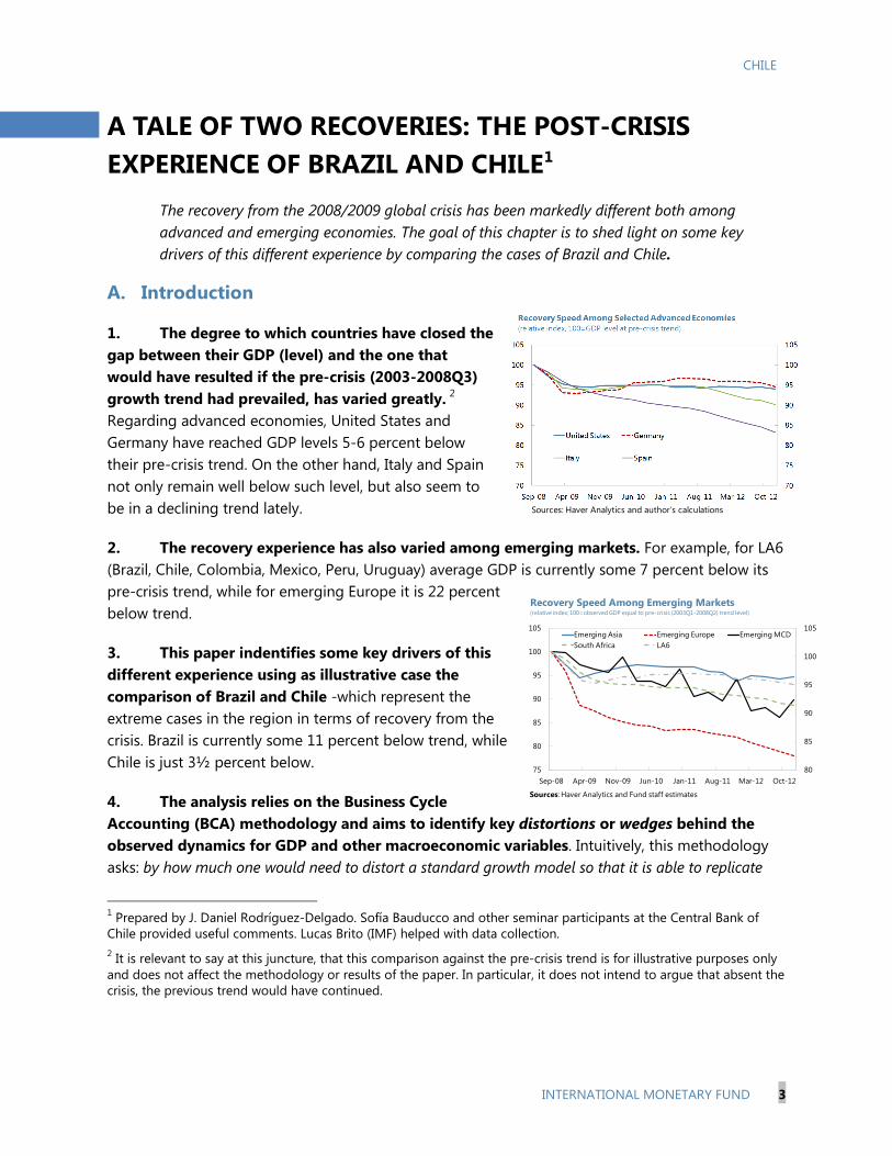
1. The degree to which countries have closed the gap between their GDP (level) and the one that would have resulted if the pre-crisis (2003-2008Q3) growth trend had prevailed, has varied greatly. 2

2. The recovery experience has also varied among emerging markets. For example, for LA6 (Brazil, Chile, Colombia, Mexico, Peru, Uruguay) average GDP is currently some 7 percent below its

Regarding advanced economies, United States and Germany have reached GDP levels 5-6 percent below their pre-crisis trend. On the other hand, Italy and Spain not only remain well below such level, but also seem to be in a declining trend lately.

pre-crisis trend, while for emerging Europe it is 22 percent below trend.

3. This paper indentifies some key drivers of this different experience using as illustrative case the comparison of Brazil and Chile -which represent the extreme cases in the region in terms of recovery from the crisis. Brazil is currently some 11 percent below trend, while Chile is just 3½ percent below.

4. The analysis relies on the Business Cycle Accounting (BCA) methodology and aims to identify key distortions or wedges behind the observed dynamics for GDP and other macroeconomic variables. Intuitively, this methodology asks: by how much one would need to distort a standard growth model so that it is able to replicate

1 Prepared by J. Daniel Rodríguez-Delgado. Sofía Bauducco and other seminar participants at the Central Bank of Chile provided useful comments. Lucas Brito (IMF) helped with data collection. 2 It is relevant to say at this juncture, that this comparison against the pre-crisis trend is for illustrative purposes only and does not affect the methodology or results of the paper. In particular, it does not intend to argue that absent the crisis, the previous trend would have continued.

Sources: Haver Analytics and author’s calculations

CHILE


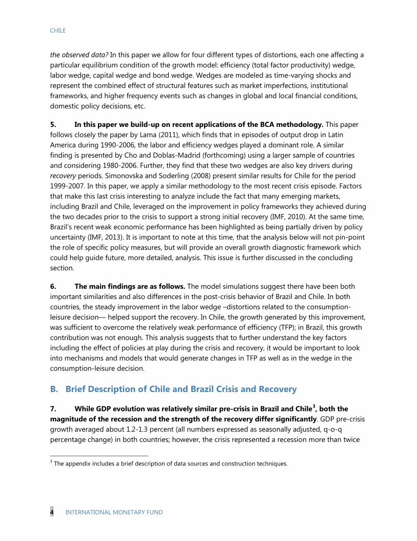
the observed data? In this paper we allow for four different types of distortions, each one affecting a particular equilibrium condition of the growth model: efficiency (total factor productivity) wedge, labor wedge, capital wedge and bond wedge. Wedges are modeled as time-varying shocks and represent the combined effect of structural features such as market imperfections, institutional frameworks, and higher frequency events such as changes in global and local financial conditions, domestic policy decisions, etc.

5. In this paper we build-up on recent applications of the BCA methodology. This paper follows closely the paper by Lama (2011), which finds that in episodes of output drop in Latin America during 1990-2006, the labor and efficiency wedges played a dominant role. A similar finding is presented by Cho and Doblas-Madrid (forthcoming) using a larger sample of countries and considering 1980-2006. Further, they find that these two wedges are also key drivers during recovery periods. Simonovska and Soderling (2008) present similar results for Chile for the period 1999-2007. In this paper, we apply a similar methodology to the most recent crisis episode. Factors that make this last crisis interesting to analyze include the fact that many emerging markets, including Brazil and Chile, leveraged on the improvement in policy frameworks they achieved during the two decades prior to the crisis to support a strong initial recovery (IMF, 2010). At the same time, Brazil’s recent weak economic performance has been highlighted as being partially driven by policy uncertainty (IMF, 2013). It is important to note at this time, that the analysis below will not pin-point the role of specific policy measures, but will provide an overall growth diagnostic framework which could help guide future, more detailed, analysis. This issue is further discussed in the concluding section.

6. The main findings are as follows. The model simulations suggest there have been both important similarities and also differences in the post-crisis behavior of Brazil and Chile. In both countries, the steady improvement in the labor wedge –distortions related to the consumption-leisure decision— helped support the recovery. In Chile, the growth generated by this improvement, was sufficient to overcome the relatively weak performance of efficiency (TFP); in Brazil, this growth contribution was not enough. This analysis suggests that to further understand the key factors including the effect of policies at play during the crisis and recovery, it would be important to look into mechanisms and models that would generate changes in TFP as well as in the wedge in the consumption-leisure decision.

B. Brief Description of Chile and Brazil Crisis and Recovery

7. While GDP evolution was relatively similar pre-crisis in Brazil and Chile3

3 The appendix includes a brief description of data sources and construction techniques.

, both the magnitude of the recession and the strength of the recovery differ significantly. GDP pre-crisis growth averaged about 1.2-1.3 percent (all numbers expressed as seasonally adjusted, q-o-q percentage change) in both countries; however, the crisis represented a recession more than twice

CHILE


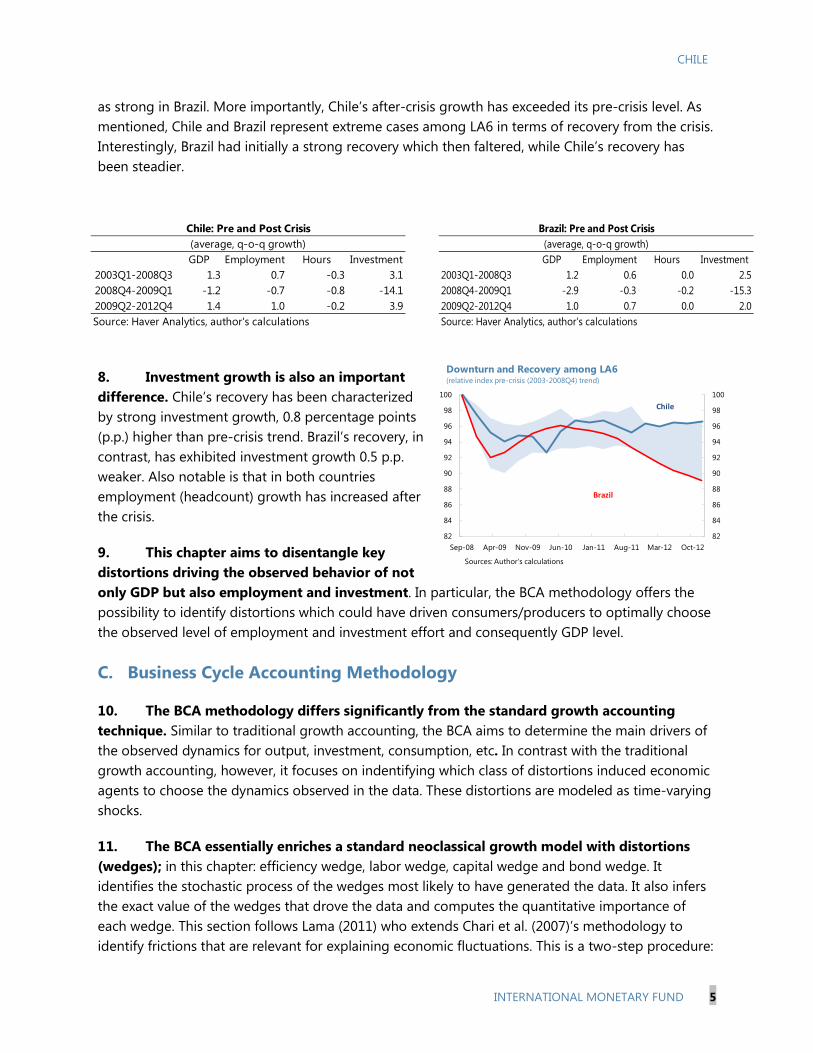
as strong in Brazil. More importantly, Chile’s after-crisis growth has exceeded its pre-crisis level. As mentioned, Chile and Brazil represent extreme cases among LA6 in terms of recovery from the crisis. Interestingly, Brazil had initially a strong recovery which then faltered, while Chile’s recovery has been steadier.

8. Investment growth is also an important difference. Chile’s recovery has been characterized by strong investment growth, 0.8 percentage points (p.p.) higher than pre-crisis trend. Brazil’s recovery, in contrast, has exhibited investment growth 0.5 p.p. weaker. Also notable is that in both countries employment (headcount) growth has increased after the crisis.

9. This chapter aims to disentangle key distortions driving the observed behavior of not only GDP but also employment and investment. In particular, the BCA methodology offers the possibility to identify distortions which could have driven consumers/producers to optimally choose the observed level of employment and investment effort and consequently GDP level.

C. Business Cycle Accounting Methodology

10. The BCA methodology differs significantly from the standard growth accounting technique. Similar to traditional growth accounting, the BCA aims to determine the main drivers of the observed dynamics for output, investment, consumption, etc. In contrast with the traditional growth accounting, however, it focuses on indentifying which class of distortions induced economic agents to choose the dynamics observed in the data. These distortions are modeled as time-varying shocks.

11. The BCA essentially enriches a standard neoclassical growth model with distortions (wedges); in this chapter: efficiency wedge, labor wedge, capital wedge and bond wedge. It identifies the stochastic process of the wedges most likely to have generated the data. It also infers the exact value of the wedges that drove the data and computes the quantitative importance of each wedge. This section follows Lama (2011) who extends Chari et al. (2007)’s methodology to identify frictions that are relevant for explaining economic fluctuations. This is a two-step procedure:

GDP Employment Hours Investment2003Q1-2008Q3 1.3 0.7 -0.3 3.12008Q4-2009Q1 -1.2 -0.7 -0.8 -14.12009Q2-2012Q4 1.4 1.0 -0.2 3.9

Chile: Pre and Post Crisis(average, q-o-q growth)

Source: Haver Analytics, author's calculations

GDP Employment Hours Investment2003Q1-2008Q3 1.2 0.6 0.0 2.52008Q4-2009Q1 -2.9 -0.3 -0.2 -15.32009Q2-2012Q4 1.0 0.7 0.0 2.0Source: Haver Analytics, author's calculations

(average, q-o-q growth)Brazil: Pre and Post Crisis

82

84

86

88

90

92

94

96

98

100

82

84

86

88

90

92

94

96

98

100


Downturn and Recovery among LA6(relative index pre-crisis (2003-2008Q4) trend)

Sources: Author's calculations

Brazil

Chile

CHILE


1) measure the wedges or deviations between the standard neoclassical growth model and the data; 2) evaluate the quantitative relevance of each individual wedge to account for the observed evolution of GDP.

12. While both the growth accounting and the BCA techniques aim to decompose observed dynamics into its subcomponents, there are important differences in how they disentangle the role of “fundamentals”. In short, the BCA aims to incorporate the role of economic agents’ decisions, while the growth accounting technique offers a more algebraic decomposition that abstracts from the fact that agents would have chosen different consumption, investment and labor decisions if the fundamentals were different.

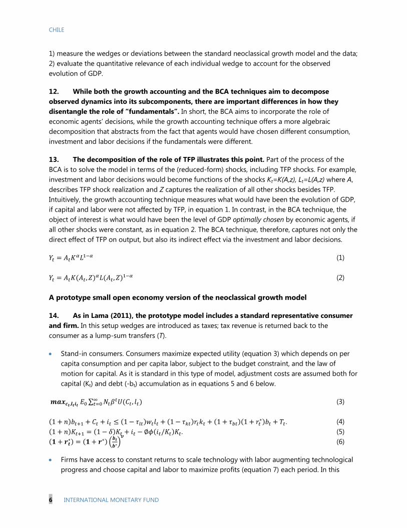
13. The decomposition of the role of TFP illustrates this point. Part of the process of the BCA is to solve the model in terms of the (reduced-form) shocks, including TFP shocks. For example, investment and labor decisions would become functions of the shocks Kt=K(A,z), Lt=L(A,z) where A, describes TFP shock realization and Z captures the realization of all other shocks besides TFP. Intuitively, the growth accounting technique measures what would have been the evolution of GDP, if capital and labor were not affected by TFP, in equation 1. In contrast, in the BCA technique, the object of interest is what would have been the level of GDP optimally chosen by economic agents, if all other shocks were constant, as in equation 2. The BCA technique, therefore, captures not only the direct effect of TFP on output, but also its indirect effect via the investment and labor decisions.

𝑌𝑡 = 𝐴𝑡𝐾𝛼𝐿1−𝛼 (1)

𝑌𝑡 = 𝐴𝑡𝐾(𝐴𝑡,𝑍)𝛼𝐿(𝐴𝑡,𝑍)1−𝛼 (2)

A prototype small open economy version of the neoclassical growth model

14. As in Lama (2011), the prototype model includes a standard representative consumer and firm. In this setup wedges are introduced as taxes; tax revenue is returned back to the consumer as a lump-sum transfers (T).

• Stand-in consumers. Consumers maximize expected utility (equation 3) which depends on per capita consumption and per capita labor, subject to the budget constraint, and the law of motion for capital. As it is standard in this type of model, adjustment costs are assumed both for capital (Kt) and debt (-bt) accumulation as in equations 5 and 6 below.

𝒎𝒂𝒙𝒄𝒕,𝒍𝒕𝒊𝒕 𝐸0 ∑ 𝑁𝑡𝛽𝑡𝑈(𝐶𝑡, 𝑙𝑡∞𝑡=0 ) (3)

(1 + 𝑛)𝑏𝑡+1 + 𝐶𝑡 + 𝑖𝑡 ≤ (1− 𝜏𝑙𝑡)𝑤𝑡𝑙𝑡 + (1− 𝜏𝑘𝑡)𝑟𝑡𝑘𝑡 + (1 + 𝜏𝑏𝑡)(1 + 𝑟𝑡∗)𝑏𝑡 + 𝑇𝑡. (4) (1 + 𝑛)𝐾𝑡+1 = (1− 𝛿)𝐾𝑡 + 𝑖𝑡 − ∅𝜙(𝑖𝑡/𝐾𝑡)𝐾𝑡. (5) (𝟏+ 𝒓𝒕∗) = (𝟏+ 𝒓∗) �𝒃𝒕

𝒃∗�𝒗

(6)

• Firms have access to constant returns to scale technology with labor augmenting technological progress and choose capital and labor to maximize profits (equation 7) each period. In this

CHILE


specification, (1+γ) is the rate of labor augmenting technical progress – assumed to be constant over time. At is the efficiency wedge.

𝜋 = 𝐴𝑡𝐹(𝐾𝑡, (1 + 𝛾)𝑡𝑙𝑡)−𝑤𝑡𝑙𝑡 − 𝑟𝑡𝑘𝑡 (7)

15. The key equilibrium conditions determining the wedges can be summarized by the following equations:

• Investment wedge: distortions to the inter-temporal allocation of consumption and investment. Models in which the availability of financing to capital investors depend on their net worth (e.g. models with default in which a higher net worth would make default less likely) are relevant candidates to generate this type of friction.

)}]1()1{([ 1111 δτβ −+−= ++++ kttktctct FAUEU (8)

• Labor wedge: distortions to the intra-temporal allocation of leisure and consumption. In the literature there a few mechanisms which have been shown to generate this type of distortions including those related to wage markups created by sticky wages or strong labor unions (Chari, et al., 2007). Neumeyer and Perri (2005) put forward an alternative mechanism based on working capital requirements. Under this mechanism, the firms total labor costs would also include a financial component so that more restrictive access to credit would represent a worsening of the labor wedge (Lama, 2011).

lttltct

lt FAUU )1( τ−=− (9)

• Efficiency wedge (TFP): gap between GDP and the combination of capital and labor. This represents the standard exogenous TFP shock commonly used in the literature. However, it is relevant to consider models that would generate this wedge endogenously. For example, trade frictions could limit firms’ exposure to foreign technology and knowledge. Matching/pairing frictions in the labor market could also result in a suboptimal allocation of skills resulting in lower observed TFP. At this moment, it is useful to note that the previous example represents one in which, a labor market-related distortion would manifest itself beyond what in this chapter is labeled as labor wedge.

t

tt F

YA = (10)

• Bond wedge: distortions to the debt accumulation decision. For example, this wedge could reflect risk premium, or the presence of enforcement-related borrowing constraints.

)}]1)(1{([ 1*

11 +++ ++= tbtctct rUEU τβ (11)

16. Although it is useful to think of them as taxes, these wedges could also represent additional factors. That is, wedges are not primitive shocks but rather reduced form representations.

CHILE


Calibration and estimation of the model

17. The calibration and estimation of the model are as follows:

• We assume a Cobb-Douglas production function and a utility function of the form:

𝑈(𝑐, 𝑙) = log 𝑐 + 𝜓log (1− 𝑙) (12)

• The capital adjustment cost is defined by

𝜙 �𝑖𝑘� = 𝑎

2( 𝑖𝑘− 𝛿 − Υ− 𝜂 − 𝑦𝜂)2 (13)

• The stochastic processes is modeled as a VAR (1):

𝑍𝑡 = [log �𝐴𝑡𝐴� , log( 1−𝜏𝑙𝑡

1−𝜏𝑖𝑡), log �1−𝜏𝑘𝑡

1−𝜏𝑘� , log (1+𝜏𝑏𝑡

1+𝜏𝑏)] (14)

𝑍𝑡 = 𝐴𝑍𝑡−1 + 𝜀𝑡 (15)

• The shocks are iid and have a standard normal distribution. From this point forward, all variables are expressed in detrended per capita (in fact, per working age population) terms, with the exception of labor/employment.

18. The general identification strategy is to calibrate the parameters of the model related to technology, preferences, and population growth, and estimate the parameters of the stochastic processes with maximum likelihood. Some of the parameters are calibrated to match the main features of Chile’s and Brazil’s quarterly data; otherwise we use values used in the literature. Ψ is calibrated based on the employment to working age population ratio and hours. The discount factor β is calibrated from the Euler equation (8) at steady state. Capital shares are inferred from Loayza, et al, 2005 (c.f. Sosa, et al, forthcoming). The rate of technological progress (γ) and population growth are calculated from each country’s data. We use a standard annual depreciation rate of 5 percent and calibrate the capital adjustment cost as in Lama (2011). The model is log-linearized around the steady state.

CHILE


D. Results

19. In his section we apply the calibrated and estimated parameters to recover values for the various wedges consistent with the data. We then infer the relative importance of the various wedges to output, employment and investment fluctuations.

20. The simulations depict the counterfactual level of GDP (investment or employment) in the case that only the specified wedge is as estimated, and all others wedges are constant at their steady state level. As explained before, wedges represent reduced-form representations of distortions in the intra and inter-temporal allocation of resources. A model with null-wedges would generate constant series in which each variable (GDP, investment, labor, and consumption) would be equal to its steady state level.

GDP decline and recovery

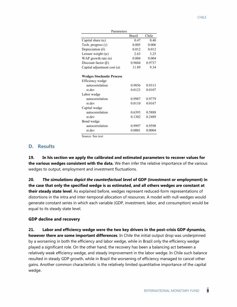
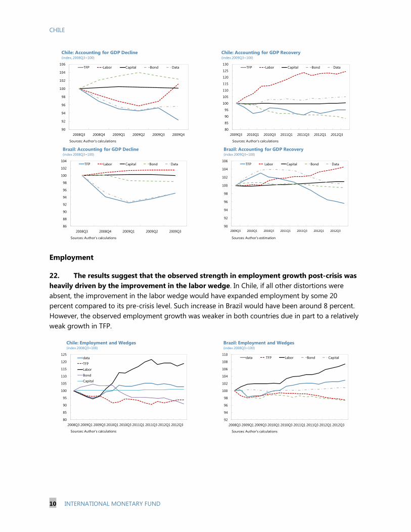
21. Labor and efficiency wedge were the two key drivers in the post-crisis GDP dynamics, however there are some important differences. In Chile the initial output drop was underpinned by a worsening in both the efficiency and labor wedge, while in Brazil only the efficiency wedge played a significant role. On the other hand, the recovery has been a balancing act between a relatively weak efficiency wedge, and steady improvement in the labor wedge. In Chile such balance resulted in steady GDP growth, while in Brazil the worsening of efficiency managed to cancel other gains. Another common characteristic is the relatively limited quantitative importance of the capital wedge.

Brazil ChileCapital share (α) 0.47 0.40Tech. progress (γ) 0.005 0.006Depreciation (δ) 0.012 0.012Leisure weight (ψ) 2.63 3.25WAP growth rate (n) 0.004 0.004Discount factor (β) 0.9604 0.9737Capital adjustment cost (a) 11.89 9.34

Efficiency wedge autocorrelation 0.9856 0.9313st.dev 0.0123 0.0107

Labor wedge autocorrelation 0.9987 0.9779st.dev 0.0110 0.0167

Capital wedge autocorrelation 0.6393 0.5888st.dev 0.1302 0.2489

Bond wedge autocorrelation 0.9997 0.9598st.dev 0.0001 0.0004

Source: See text

Parameters

Wedges Stochastic Process

CHILE


Employment

22. The results suggest that the observed strength in employment growth post-crisis was heavily driven by the improvement in the labor wedge. In Chile, if all other distortions were absent, the improvement in the labor wedge would have expanded employment by some 20 percent compared to its pre-crisis level. Such increase in Brazil would have been around 8 percent. However, the observed employment growth was weaker in both countries due in part to a relatively weak growth in TFP.

90

92

94

96

98

100

102

104

106

2008Q3 2008Q4 2009Q1 2009Q2 2009Q3 2009Q4

TFP Labor Capital Bond Data

Chile: Accounting for GDP Decline(index, 2008Q3=100)


80

85

90

95

100

105

110

115

120

125

130

2009Q3 2010Q1 2010Q3 2011Q1 2011Q3 2012Q1 2012Q3


Chile: Accounting for GDP Recovery(index 2009Q3=100)


86

88

90

92

94

96

98

100

102

104

2008Q3 2008Q4 2009Q1 2009Q2 2009Q3


Brazil: Accounting for GDP Decline(index 2008Q3=100)


90

92

94

96

98

100

102

104

106

2009Q3 2010Q1 2010Q3 2011Q1 2011Q3 2012Q1 2012Q3


Brazil: Accounting for GDP Recovery(index 2009Q3=100)

Sources: Author's estimation

80

85

90

95

100

105

110

115

120

125

2008Q3 2009Q1 2009Q3 2010Q1 2010Q3 2011Q1 2011Q3 2012Q1 2012Q3

data

TFP

Labor

Bond

Capital

Chile: Employment and Wedges(index 2008Q3=100)


92

94

96

98

100

102

104

106

108

110

2008Q3 2009Q1 2009Q3 2010Q1 2010Q3 2011Q1 2011Q3 2012Q1 2012Q3

data TFP Labor Bond Capital

Brazil: Employment and Wedges(index 2008Q3=100)


CHILE


Investment

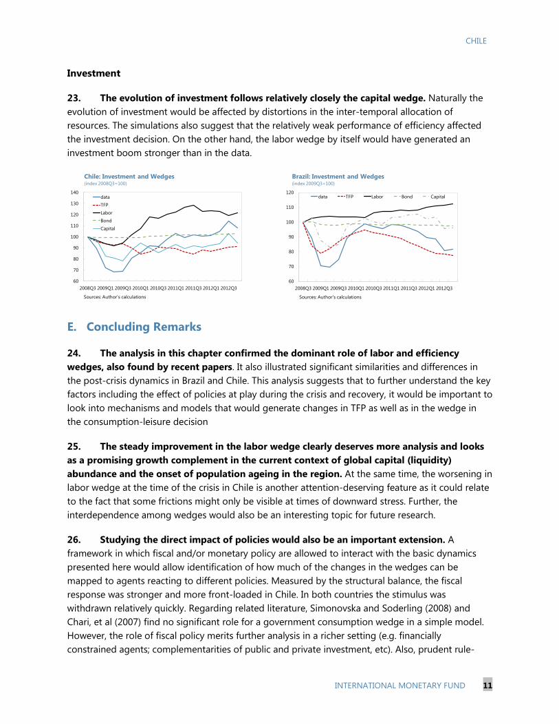
23. The evolution of investment follows relatively closely the capital wedge. Naturally the evolution of investment would be affected by distortions in the inter-temporal allocation of resources. The simulations also suggest that the relatively weak performance of efficiency affected the investment decision. On the other hand, the labor wedge by itself would have generated an investment boom stronger than in the data.

E. Concluding Remarks

24. The analysis in this chapter confirmed the dominant role of labor and efficiency wedges, also found by recent papers. It also illustrated significant similarities and differences in the post-crisis dynamics in Brazil and Chile. This analysis suggests that to further understand the key factors including the effect of policies at play during the crisis and recovery, it would be important to look into mechanisms and models that would generate changes in TFP as well as in the wedge in the consumption-leisure decision

25. The steady improvement in the labor wedge clearly deserves more analysis and looks as a promising growth complement in the current context of global capital (liquidity) abundance and the onset of population ageing in the region. At the same time, the worsening in labor wedge at the time of the crisis in Chile is another attention-deserving feature as it could relate to the fact that some frictions might only be visible at times of downward stress. Further, the interdependence among wedges would also be an interesting topic for future research.

26. Studying the direct impact of policies would also be an important extension. A framework in which fiscal and/or monetary policy are allowed to interact with the basic dynamics presented here would allow identification of how much of the changes in the wedges can be mapped to agents reacting to different policies. Measured by the structural balance, the fiscal response was stronger and more front-loaded in Chile. In both countries the stimulus was withdrawn relatively quickly. Regarding related literature, Simonovska and Soderling (2008) and Chari, et al (2007) find no significant role for a government consumption wedge in a simple model. However, the role of fiscal policy merits further analysis in a richer setting (e.g. financially constrained agents; complementarities of public and private investment, etc). Also, prudent rule-

60

70

80

90

100

110

120

130

140

2008Q3 2009Q1 2009Q3 2010Q1 2010Q3 2011Q1 2011Q3 2012Q1 2012Q3

data

TFP

Labor

Bond

Capital

Chile: Investment and Wedges(index 2008Q3=100)


60

70

80

90

100

110

120

2008Q3 2009Q1 2009Q3 2010Q1 2010Q3 2011Q1 2011Q3 2012Q1 2012Q3

data TFP Labor Bond Capital

Brazil: Investment and Wedges(index 2009Q3=100)


CHILE


based fiscal behavior, as in Brazil and Chile, could be an important determinant of inter-temporal decisions such as investment which could be otherwise being measured in the investment wedge. Regarding monetary policy in Chile, it was first tightened–in the context of relatively high inflation- during September 08-January 09 and later on aggressively loosened; while Brazil had a smoother sequence of rate cuts. Also striking is the strong policy easing since late-2011 in Brazil, while in Chile the rate has been reverted to its pre-crisis level. Financial conditions could be affecting not only the investment wedge but also the labor wedge as explained.

27. The wedges specification can also be enriched. In the framework presented in this chapter, the stochastic process governing the wedges is assumed constant throughout the sample period. However, it would be interesting to explore the role of higher uncertainty or other structural breaks during or after the crisis. Changes in expectations could be an important factor for what is here being measured in this chapter as efficiency and/or investment wedge.

-8

-7

-6

-5

-4

-3

-2

-1

0

1

2

3

-8

-7

-6

-5

-4

-3

-2

-1

0

1

2

3


Chile Brazil

Brazil and Chile: Monetary Policy Response(real policy rates; p.p. deviation from September 08)

Sources: Haver Analytics and Fund staff estimates

-4

-3

-2

-1

0

1

2

3

-4

-3

-2

-1

0

1

2

3

2008 2009 2010 2011 2012 2013

Chile Brazil

Brazil and Chile: Fiscal Policy Respose(change in structural balance, -=expansionary; in percent of GDP)

Sources: World Economic Outlook and Fund staff estimates

CHILE


Appendix

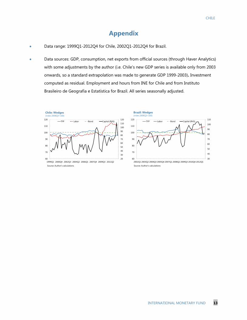
• Data range: 1999Q1-2012Q4 for Chile, 2002Q1-2012Q4 for Brazil.

• Data sources: GDP, consumption, net exports from official sources (through Haver Analytics)

with some adjustments by the author (i.e. Chile’s new GDP series is available only from 2003

onwards, so a standard extrapolation was made to generate GDP 1999-2003). Investment

computed as residual. Employment and hours from INE for Chile and from Instituto

Brasileiro de Geografia e Estatística for Brazil. All series seasonally adjusted.

30

40

50

60

70

80

90

100

110

60

70

80

90

100

110

120

2002Q1 2003Q2 2004Q3 2005Q4 2007Q1 2008Q2 2009Q3 2010Q4 2012Q1

TFP Labor Bond Capital (RHS)

Brazil: Wedges(index 2008Q3=100)

Source: Author's calculations

20

30

40

50

60

70

80

90

100

110

120

60

70

80

90

100

110

120

1999Q1 2000Q4 2002Q3 2004Q2 2006Q1 2007Q4 2009Q3 2011Q2

TFP Labor Bond Capital (RHS)

Chile: Wedges(index 2008Q3=100)

Source: Author's calculations

CHILE


References

Chari, V.V., Kehoe, P.J., McGrattan, E.R., 2007, ”Business Cycle Accounting”. Econometrica 75 (3), 781-836.

Cho, D., Doblas-Madrid, A., forthcoming, “Business cycle accounting East and West: Asian finance and the investment wedge”, Review of Economic Dynamics

IMF, 2010, “World Economic Outlook: Recovery, Risk and Rebalancing.” World Economic and Financial Surveys

IMF, 2013, “World Economic Outlook: Hopes, Reality, Risks.” World Economic and Financial Surveys

Lama, R., 2011, “Accounting for output drops in Latin America”. Review of Economic Dynamics Vol 14, pp. 295-316.

Loayza, N., Fajnzylber, P. and Calderón,C. 2005, Economic Growth in Latin America and the Caribbean: Stylized Facts, Explanations, and Forecasts, World Bank.

Neumeyer, P., Perri, F., 2005. “Business cycles in emerging economies: The role of interest rates”. Journal of Monetary Economics 52, 345–380

Simonovska, I. Soderling, L, 2008, “Business Cycle Accounting for Chile”, IMF Working Papers 08/61

Sosa, S., Tsounta, E., Kim, H., forthcoming, “Is the Growth Momentum in Latin America Sustainable?”, IMF Working Papers.

CHILE


SYSTEMIC RISK ASSESSMENT AND MITIGATION IN CHILE1

Systemic risk assessment and mitigation tools are an integral part of a macroprudential policy framework. This chapter provides a quantitative framework for systemic risk monitoring in Chile and discusses the Chilean macroprudential toolkit.

A. Systemic Risk Assessment

1. This section provides a framework for systemic risk monitoring for Chile. It focuses on quantitative approaches to systemic risk. Two challenges should be acknowledged. First, in practice, these quantitative tools need to be complemented with qualitative assessments. Second, progress in quantitative risk assessments depends on data availability.

2. In monitoring systemic risk, it is important to consider both the time and the cross-sectional dimensions.

• Time dimension. Risk is built up over the macroeconomic cycle with a procyclical bias, as financial institutions tend to take on excessive risks in the upswing of an economic cycle only to become overly risk-averse in a down-swing. This characteristic amplifies the boom and bust cycle.

• Cross-sectional dimension. The growing complexity of the financial system is raising interconnectedness and common exposures conducive to rapid contagion risk when crises occur. Shocks are amplified and transmitted rapidly between financial institutions. Moreover, the failure of one systemically important financial institution can threaten the system as a whole.

3. This chapter focuses on the time dimension of systemic risk. The analysis focuses first on the behavior of credit aggregates, and is then complemented with other macroeconomic and financial variables. For an analysis of the cross-sectional dimension of systemic risk in Chile, see Chan-Lau 2009 and 2010 that focus on price-based and balance-sheet network analysis.

Single indicator (credit)

4. Economic activity and credit fluctuations are closely linked through wealth effects and the financial accelerator mechanism. In an upturn, better growth prospects improve borrower creditworthiness and collateral values. Lenders respond with an increased supply of credit and, sometimes, looser credit standards. More abundant credit allows for greater investment and

1 Prepared by Nicolas Arregui. Alejandro Jara and other seminar participants at the Central Bank of Chile provided useful comments.

CHILE


consumption and further increases collateral values. In a downturn, the process is reversed. Theory has identified several channels that may lead to excessive risk taking during episodes of rapid credit growth.2

5. A large and growing literature identifies credit growth as a powerful predictor of financial crises. The empirical literature identifies credit booms as “significant” deviations above trend using different methodologies to compute the trend and different thresholds that determine a boom. Nonetheless, the finding that credit significantly above trend is a good predictor of financial crises is pretty robust across methodologies and thresholds. This chapter considers a variety of methodologies to measure credit conditions.

Such channels can explain why “the worst loans are made at the top of the business cycle” and justify policy intervention to prevent excessive risk taking during the boom. Also, the rapid growth of the loan base may mask an underlying deterioration of loan quality.

• GFSR (2011) finds that increases in the credit-to-GDP ratio of more than 3 percentage points, year-on-year, is a good early warning signal one to two years before a financial crisis.

• Mendoza and Terrones (2008) identify a credit boom when the deviation from the long–run trend in the logarithm of real credit per capita exceeds 1.75 times the standard deviation of the cyclical component. The long-run trend is calculated using the Hodrick-Prescott (HP) filter with the smoothing parameter set at 100, as is typical for annual data.

• Borio-Lowe-Drehman (2002,2009) conclude that among several variables, the “credit gap”, based on the credit-to-GDP ratio, is the most powerful indicator for banking crises. They estimate such a gap by extracting the trend (interpreted as the equilibrium credit-to GDP ratio) from the ratio using the HP filter with relatively high smoothing parameters (lambda equal to 1600 instead of 100 for annual data).

• Dell’Ariccia et al (2012) define a credit gap measure as the percentage deviation of credit-to-GDP from a backward looking, rolling, cubic trend estimated over the period between t-10 and t. A credit boom occurs when the deviation from trend is greater than 1.5 times its standard deviation and the annual growth rate of the credit-to-GDP ratio exceeds 10 percent or when the annual growth rate of the credit-to-GDP ratio exceeds 20 percent.3

2 Contributing to looser lending standards and greater credit cyclicality may be managerial reputational concerns (Rajan, 1994), improved borrowers’ income prospects (Ruckes, 2004), loss of institutional memory of previous crises (Berger and Udell, 2004), expectations of government bailouts (Rancière, Tornell, and Westermann, 2008), and a decline in adverse selection costs due to improved information symmetry across banks (Dell’Ariccia and Marquez, 2006). In addition, externalities driven by strategic complementarities (such as cycles in collateral values) may lead banks to take excessive or correlated risks during the upswing of a financial cycle (De Nicolò, Favara, and Ratnovski, 2012).

3 When applying their methodology to a sample of 170 countries from 1960 to 2010, Dell’Ariccia et al. (2012) find that one in three booms ends in a banking crisis (as defined in Laeven and Valencia, 2010) within three years.

CHILE


6. Bank credit growth in Chile has been strong in the last two years. The Chilean economy recovered rapidly from the global financial crisis and the February 2010 earthquake. From mid-2010 to June 2011, the central bank raised the policy rate from 0.5 percent to 5.25 percent, helping bring inflation expectations closer to the target. Credit growth strengthened during this period, in line with income. Nominal and real credit growth have been in double digits for most of the last two years.

7. However, bank credit growth has been below most thresholds of credit booms. Credit growth has not been “excessive” as defined by the Borio-Lowe-Drehmann, the Mendoza-Terrones, or the Dell’Ariccia et al. methodologies (Figure 1). However, since September 2011, the increase in the credit-to-GDP ratio has exceeded (or nearly exceeded) the 3 percentage point threshold suggested in IMF (2011b). The GFSR threshold is more conservative than other methodologies in that it flags risks more often, predicting more crises that fail to materialize, but missing fewer crises than other methodologies.4

8. It is also important to look beyond credit extended by banks. A systemic financial risk assessment should look at all institutions that perform critical financial market functions, including credit intermediation, maturity transformation, the provision of savings vehicles, and the support of primary and secondary funding markets. In Chile, banks account for only about half of the financial system as measured by assets. The other half consists mainly of pension funds, insurance companies, and nonbank consumer outfits. The claims on the private sector by pension funds and insurance companies represent roughly 40 percent of the claims on the private sector by banks. Figure 2 applies the GFSR methodology to the broad credit-to-GDP ratio a broad measure of credit

Credit growth has been moderating but authorities should continue to monitor the evolution of credit to GDP ratio and other credit gap measures.

5

to the private sector, comprising banks, insurance companies and pension funds. Broad credit-to-GDP appears growing in line with bank credit. In particular, it has also been increasing above the 3 percentage point threshold suggested by the IMF (2011b) methodology to flag risks.6

4 See IMF (2011b) for comparison with the Borio-Lowe-Drehmann methodology and Arregui and others (forthcoming) for a comparison with the Dell’Ariccia methodology.

The flip side of increases in credit is given by the increased leverage by borrowers. Household leverage (at about

5 The series for credit is “Claims on Private Sector” in the IMF International Financial Statistics (IFS) database. 6 IFS data for Chile does not include investment funds, mutual funds, general funds, housing funds, foreign capital investment funds, factoring societies, leasing companies, and financial auxiliaries.

-4-2024681012141618

-4

-2

0

2

4

6

8

10

12

2007Q1 2008Q1 2009Q1 2010Q1 2011Q1 2012Q1

Policy rateReal GDP Growth (yoy)Real PS Credit Growth (yoy; right)

Monetary policy and growth (in percent)

Sources: IFS

CHILE


36 percent of GDP) has been stable while corporate indebtedness (90 percent of GDP) has risen; both appear in line with Chile’s level of economic development from a cross-country perspective.7

Figure 1. Chile: Assessing Credit Growth

7 Currency mismatches in corporate and household balance sheet are limited and have been broadly stable.

Sources: IFS, WDI and Fund staff calculations.

-5

0

5

10

15

20

25

2000Q12002Q12004Q12006Q12008Q12010Q12012Q1

Nominal credit growthReal credit growth

Credit Growth (yoy; in percent)

-15

-10

-5

0

5

10

15

20

25

1970 1977 1984 1991 1998 2005 2012

3pp threshold

Change in credit-to-GDP

GFSR methodology(in percentage points)

-20

-10

0

10

20

30

40

1970 1977 1984 1991 1998 2005 2012

Lambda=100

Lambda=1600

2pp

10pp

Borio-Lowe-Drehmann methodology(credit to GDP gap; in percentage points)

-15

-10

-5

0

5

10

1970 1977 1984 1991 1998 2005 2012

Cyclical component

1.75 times Std. Dev.

Mendoza-Terrones methodology(real per capita credit; deviation from trend in percent )

-20

-10

0

10

20

30

40

50

60

1971 1978 1985 1992 1999 2006

Credit-to-GDP growth10pp20pp

Dell'Ariccia and others methodology (I)(growth rate in credit to GDP; in percent)

-20

-15

-10

-5

0

5

10

15

20

25

1971 1978 1985 1992 1999 2006

Cyclical component

1.5* std dev of cyclical component

Dell'Aricca and others methodology (II)(credit to GDP gap; in percentage points)

CHILE


Figure 2. Chile: Broad Credit Growth

1/ Narrow credit is defined as Claims on the Private Sector by Other Depository Corporations (ODC). Broad Credit is defined as Claims on the Private Sector by Other Financial Corporations (OFC). In the case of Chile, ODC include banks and OFC include pension funds and insurance companies.

0102030405060708090

100

Chile

Braz

il

Colo

mbi

a

Uru

guay

Mex

ico

Arge

ntin

a

BanksBanks and other financial corporations

Broad and Narrow Credit to Private Sector /1 (in percent of GDP; 2011)

-6

-4

-2

0

2

4

6

8

10

2009Q1 2009Q4 2010Q3 2011Q2 2012Q1

Change in Narrow Credit to GDP (yoy)3 pp thresholdChange in Broad Credit to GDP (yoy)

Change in Broad and Narrow Credit to GDP(yoy change; in percentage points)

36.5

32

33

34

35

36

37

38

2008Q4 2009Q3 2010Q2 2011Q1 2011Q4 2012Q3

Household (includes all liabilities)

Household indebtedness (in percent of annual GDP; data up to 2012Q3)

Sources: IFS and Banco Central de Chile.

89.1

727476788082848688909294

2008Q4 2009Q3 2010Q2 2011Q1 2011Q4 2012Q3

Corporate

Corporate indebtedness (in percent of annual GDP; data up to 2012Q3)

CHILE


Multiple indicators

9. Analyzing the joint behavior of credit and other macroeconomic and financial indicators generally provides a better signal than just looking at credit.

• Borio and Lowe (2002), Borio and Drehmann (2009) and IMF (2011b) show that combinations of credit and asset price deviations from long-term trends are the best leading indicator of banking distress. Reinhart and Rogoff (2009) and Barrel et al (2010) provide further evidence on the ability of housing prices to predict financial crises. GFSR 2011 shows that, in emerging economies, the real effective exchange rate (REER) tends to appreciate rapidly in the run-up to a crisis.

• Kaminsky and Reinhart (1999) and Barrel et al (2010) find evidence that current account deficits can predict banking crises. However, when accounting for both current account deficits and credit growth, Jorda et al (2011) show that credit growth emerges as the single best predictor of financial instability. In recent decades, the correlation between lending booms and current account imbalances has grown much tighter.

10. In Chile, additional macroeconomic and financial indicators do not indicate an elevated systemic risk, but suggest some channels to require continued monitoring by authorities. We follow Borio-Lowe-Drehmann trying to detect the symptoms of the build-up of financial imbalances in monitoring unusually rapid and sustained growth in credit and in asset prices. For some small open economies, the cumulative appreciation of the real exchange rate might also be helpful. It could capture the pressure associated with capital inflows as well as the potential build-up of concomitant foreign exchange mismatches. Because time series for Chile are relatively short8 , this note centers the analysis on growth rates instead of deviations from trend, in line with Fitch Ratings methodology to compute a Macro Prudential Index (MPI).9

• Stock prices. The behavior in the Santiago Stock Exchange IPSA index

Figure 3 shows the growth rates together with the indicative thresholds to flag risks suggested by Fitch ratings.

10

8 Equity price index is available only since 1990 and housing prices are available only since 2002.

does not show any sign of asset boom and does not appear to be an increasing vulnerability that could potentially feed back into the real economy and financial sector.

9 Fitch Ratings computes a Macro Prudential Index (MPI) that identifies the build-up of potential stress in banking systems due to rapid credit growth associated with bubbles in housing markets, equity markets or real exchange rates. High vulnerability to potential systemic stress is defined as: (i) real private sector credit growth exceeding an average 15 percent a year over two years, and; (ii) real property price growth of more than five percent a year in the same period, or; (iii) real effective exchange rate appreciation of more than four percent a year in the same period, or; real equity price growth of more than 17 percent a year (in the preceding two years). 10 The IPSA Index is a Total Return Index and is composed of the 40 stocks with the highest average annual trading volume in the Santiago Stock Exchange (Bolsa de Comercio de Santiago).

CHILE


Figure 3. Chile: Credit Growth and Asset Prices

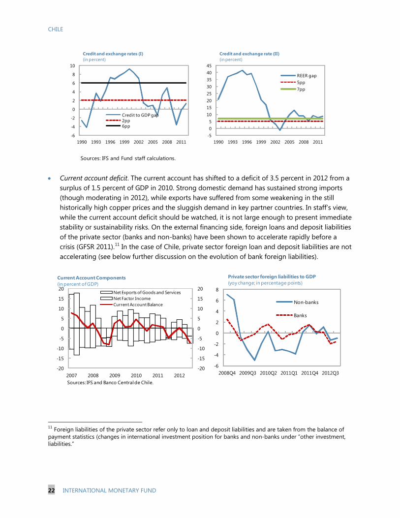
• Real effective exchange rate (REER). The peso is about 10 percent above its 1996-2012 average.

Since REER time series are available back to 1980, the gap analysis in Borio-Lowe-Drehmann can be conducted. Over the last years, the REER gap exceeds the thresholds suggested in Borio-Lowe for all countries (7 percentage points) and for emerging economies (5 percentage points). However, it should be noted that the gap measures when using shorter data series is heavily influenced by the developments in the 80s. Staff analysis (see Chile 2013 IMF Article IV Consultation staff report) finds that the peso is on the strong side though not clearly overvalued.

Source: IFS and Banco Central de Chile.

-4-202468

1012141618

Mar-03 Nov-04 Jul-06 Mar-08 Nov-09 Jul-11

Real credit growth15pp

Real credit growth(yoy; in percent)

-15

-10

-5

0

5

10

15

20


REER appreciation4pp

Real Effective Exchange Rate(yoy; in percent)

-40-30-20-10

0102030405060


IPSA deflated by inflation17pp

Asset Prices (yoy; in percent)

-6

-4

-2

0

2

4

6

8

10

12


Real residential prices (stratified)Greater Santiago real residential prices (hedonic)5pp

Housing Prices (yoy; in percent)

CHILE


• Current account deficit. The current account has shifted to a deficit of 3.5 percent in 2012 from a surplus of 1.5 percent of GDP in 2010. Strong domestic demand has sustained strong imports (though moderating in 2012), while exports have suffered from some weakening in the still historically high copper prices and the sluggish demand in key partner countries. In staff’s view, while the current account deficit should be watched, it is not large enough to present immediate stability or sustainability risks. On the external financing side, foreign loans and deposit liabilities of the private sector (banks and non-banks) have been shown to accelerate rapidly before a crisis (GFSR 2011).11

In the case of Chile, private sector foreign loan and deposit liabilities are not accelerating (see below further discussion on the evolution of bank foreign liabilities).

11 Foreign liabilities of the private sector refer only to loan and deposit liabilities and are taken from the balance of payment statistics (changes in international investment position for banks and non-banks under “other investment, liabilities.”

Sources: IFS and Fund staff calculations.

-6

-4

-2

0

2

4

6

8

10

1990 1993 1996 1999 2002 2005 2008 2011

Credit to GDP gap2pp6pp

Credit and exchange rates (I) (in percent)

-505

1015202530354045

1990 1993 1996 1999 2002 2005 2008 2011

REER gap5pp7pp

Credit and exchange rate (II) (in percent)

-6

-4

-2

0

2

4

6

8

2008Q4 2009Q3 2010Q2 2011Q1 2011Q4 2012Q3

Non-banks

Banks

Private sector foreign liabilities to GDP(yoy change; in percentage points)

-20

-15

-10

-5

0

5

10

15

20

-20

-15

-10

-5

0

5

10

15

20

2007 2008 2009 2010 2011 2012

Net Exports of Goods and ServicesNet Factor IncomeCurrent Account Balance

Current Account Components(in percent of GDP)

Sources: IFS and Banco Central de Chile.

CHILE


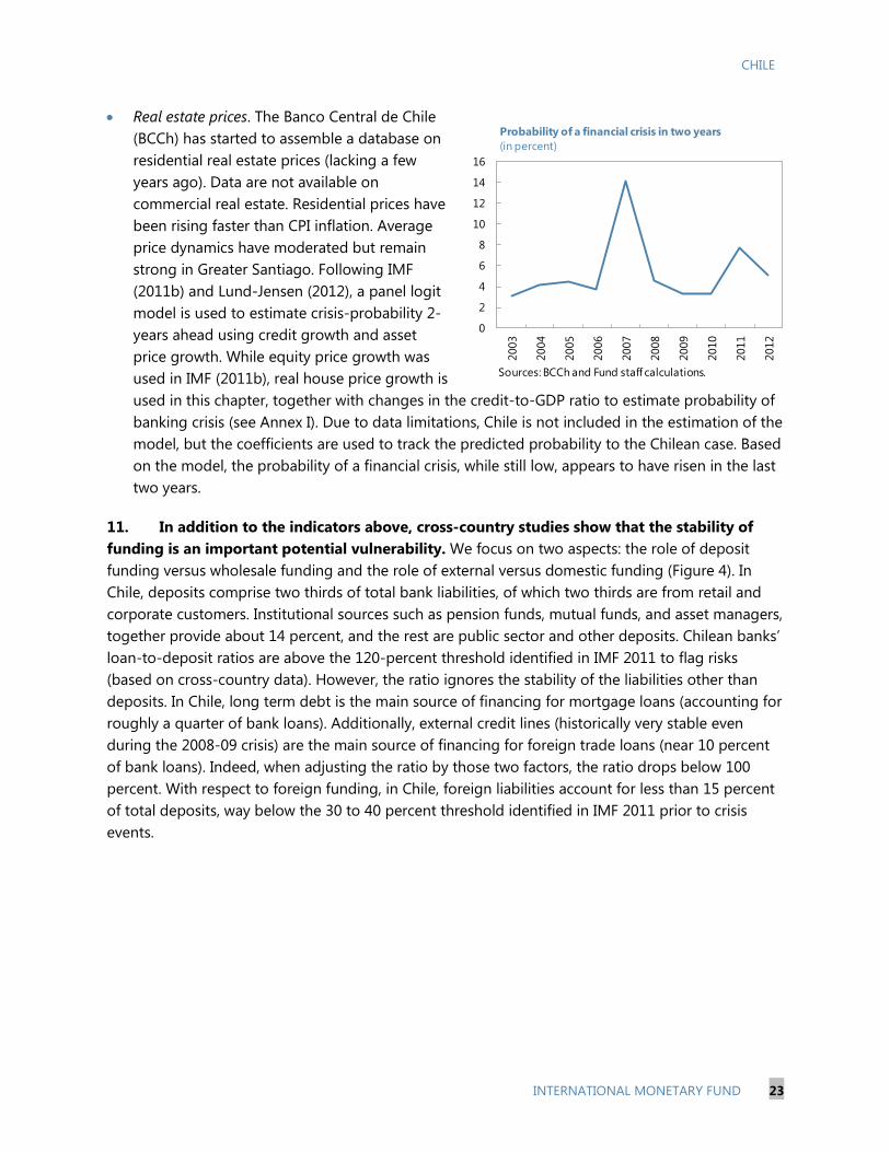
• Real estate prices. The Banco Central de Chile (BCCh) has started to assemble a database on residential real estate prices (lacking a few years ago). Data are not available on commercial real estate. Residential prices have been rising faster than CPI inflation. Average price dynamics have moderated but remain strong in Greater Santiago. Following IMF (2011b) and Lund-Jensen (2012), a panel logit model is used to estimate crisis-probability 2-years ahead using credit growth and asset price growth. While equity price growth was used in IMF (2011b), real house price growth is used in this chapter, together with changes in the credit-to-GDP ratio to estimate probability of banking crisis (see Annex I). Due to data limitations, Chile is not included in the estimation of the model, but the coefficients are used to track the predicted probability to the Chilean case. Based on the model, the probability of a financial crisis, while still low, appears to have risen in the last two years.

11. In addition to the indicators above, cross-country studies show that the stability of funding is an important potential vulnerability. We focus on two aspects: the role of deposit funding versus wholesale funding and the role of external versus domestic funding (Figure 4). In Chile, deposits comprise two thirds of total bank liabilities, of which two thirds are from retail and corporate customers. Institutional sources such as pension funds, mutual funds, and asset managers, together provide about 14 percent, and the rest are public sector and other deposits. Chilean banks’ loan-to-deposit ratios are above the 120-percent threshold identified in IMF 2011 to flag risks (based on cross-country data). However, the ratio ignores the stability of the liabilities other than deposits. In Chile, long term debt is the main source of financing for mortgage loans (accounting for roughly a quarter of bank loans). Additionally, external credit lines (historically very stable even during the 2008-09 crisis) are the main source of financing for foreign trade loans (near 10 percent of bank loans). Indeed, when adjusting the ratio by those two factors, the ratio drops below 100 percent. With respect to foreign funding, in Chile, foreign liabilities account for less than 15 percent of total deposits, way below the 30 to 40 percent threshold identified in IMF 2011 prior to crisis events.

0

2

4

6

8

10

12

14

16

2003

2004

2005

2006

2007

2008

2009

2010

2011

2012

Probability of a financial crisis in two years (in percent)

Sources: BCCh and Fund staff calculations.

CHILE


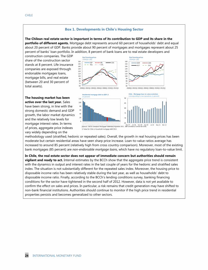
Box 1. Developments in Chile’s Housing Sector The Chilean real estate sector is important in terms of its contribution to GDP and its share in the portfolio of different agents. Mortgage debt represents around 60 percent of households’ debt and equal about 20 percent of GDP. Banks provide about 90 percent of mortgages and mortgages represent about 25 percent of banks’ loan portfolio. In addition, 8 percent of bank loans are to real estate developers and construction companies. The GDP share of the construction sector stands at 8 percent. Life insurance companies are exposed through endorsable mortgages loans, mortgage bills, and real estate (between 20 and 30 percent of total assets).

The housing market has been active over the last year. Sales have been strong, in line with the strong domestic demand and GDP growth, the labor market dynamics and the relatively low levels for mortgage interest rates. In terms of prices, aggregate price indexes vary widely depending on the methodology used (stratified, hedonic or repeated sales). Overall, the growth in real housing prices has been moderate but certain residential areas have seen sharp price increase. Loan-to-value ratios average has increased to around 85 percent (relatively high from cross country comparison). Moreover, most of the existing bank mortgages (85 percent) are non-endorsable mortgage loans, which have no regulatory loan-to-value limit.

In Chile, the real estate sector does not appear of immediate concern but authorities should remain vigilant and ready to act. Internal estimates by the BCCh show that the aggregate price trend is consistent with the dynamics in output and interest rates in the last couple of years for the hedonic and stratified sales index. The situation is not substantially different for the repeated sales index. Moreover, the housing price to disposable income ratio has been relatively stable during the last year, as well as households’ debt to disposable income ratio. Finally, according to the BCCh’s lending conditions survey, banking financing conditions for the sector have tightened in the second half of 2012. However, data is not yet available to confirm the effect on sales and prices. In particular, a risk remains that credit generation may have shifted to non-bank financial institutions. Authorities should continue to monitor if the high price trend in residential properties persists and becomes generalized to other sectors.

60708090

100110120130140150160

2000Q1 2002Q1 2004Q1 2006Q1 2008Q1 2010Q1 2012Q1

ESP IRL USANZL CHL

Real housing prices (2004Q4=100)

60708090

100110120130140150160

2000Q1 2002Q1 2004Q1 2006Q1 2008Q1 2010Q1 2012Q1

KOR CANAUT CHL

Real housing prices(2004Q4=100)

0

20

40

60

80

100

120

Residential mortgage debt to GDP /1(in percent)

65

70

75

80

85

90

Mar-07 Jan-08 Nov-08 Sep-09 Jul-10 May-11 Mar-12

Chile - Mortgage loan-to-value evolution(corresponding to new operations; in percent)

Sources : OECD, European Mortgage Federation Hypostat 2011 , SBIF and Banco Central de Chile. 1/ Value for Chile is Household mortgage debt 2012.

CHILE


Figure 4. Chile: Bank Funding Risks

1.1

1.15

1.2

1.25

1.3

1.35

1.4

1.45

1.5

Jan-00 Sep-01 May-03 Jan-05 Sep-06 May-08 Jan-10 Sep-11

Large Banks

Medium Banks

System

Loan to Deposits(units)

0.7

0.75

0.8

0.85

0.9

0.95

1

1.05

1.1

Jan-00 Sep-01 May-03 Jan-05 Sep-06 May-08 Jan-10 Sep-11

Large Banks

Medium Banks

System

Loan excl. comex to deposits and mortgage financing(units)

Sources: SBIF and Haver Analytics.

0100020003000400050006000700080009000

10000

Mar-00 Dec-01 Sep-03 Jun-05 Mar-07 Dec-08 Sep-10 Jun-12

Currency and depositsLoansMoney market

Bank Short term external debt composition(mn USD)

0

2000

4000

6000

8000

10000

12000

14000

16000

18000


Loans Bonds and notes

Bank long term external debt composition(mn USD)

0

2

4

6

8

10

12

14

16

18

Jan-09 Aug-09 Mar-10 Oct-10 May-11 Dec-11 Jul-12

to total liabilitites

to deposits

Bank foreign liabilities (in percent)

0

5000

10000

15000

20000

25000


Long term Short term

Bank external debt by maturity(mn USD)

CHILE


B. Systemic Risk Mitigation

12. Macroprudential instruments can help address potential sources of risk. Since the world is still gaining experience with macroprudential policies and since, in any event, the appropriate set and design of macroprudential tools depend on country-characteristics, there is no one set of tools and designs that can be seen as “best practice.” That said, countries can learn from budding experience of other countries.12

13. It should be noted that macroprudential policy is not well-suited to control asset prices or exchange rates.

Because the systemic risk assessment in the previous section does not find elevated systemic risks (although some channels and risks require continued monitoring), this section focuses on the development of a macroprudential toolkit and not on the activation of specific macroprudential tools.

13

14. Chile has had experience with some prudential instruments that may be used for macroprudential purposes (e.g. loan-to-value and debt-to-income requirements, liquidity requirements and exposure and currency mismatch limits). Their use for macroprudential purposes would require a more active approach, including periodic recalibration. Other instruments, particularly to address the time dimension of systemic risk (e.g. time varying capital buffers and dynamic provisioning rules), have not been used in Chile and their implementation poses more challenges (Annex II). In particular, two (now) commonly discussed instruments are not part of the Chilean macroprudential toolkit and two other instruments present some limitation that may deserve consideration:

Rather, macroprudential policy can seek to contain the vulnerability of the system to asset price reversals. It is important to distinguish between macroprudential measures and capital flow management measures (CFMs). CFMs are designed to limit capital flows and affect the exchange rate. Macroprudential measures are designed to limit systemic vulnerabilities. These can include vulnerabilities associated with capital inflows and exposure of the financial system to exchange rate shocks, but macroprudential measures do not seek to affect the inflow or the exchange rate per se.

• Dynamic provisioning. Dynamic provisioning is currently limited to voluntary provisions by banks. The individual evaluation models for unimpaired portfolio calculate provisions based on parameters like the probability of default and loss given default. Both parameters are defined in advance by the Supervisor, and are set at long-term estimates (representative of at least one cycle). Chan-Lau (2012) runs a simulation exercise for Chile and finds that Spanish dynamic

12 Lim et al. (2011) find that several macroprudential tools can reduce credit growth procyclicality. Arregui et al. (forthcoming) find that a variety of macroprudential tools has direct impact on banking aggregates such as credit growth. Almeida, Campello and Liu (2005), Wong et al (2011), Ahuja and Nabar (2011), IMF (2011d) and Kuttner and Shim (2012) study the effectiveness of LTV limits. Vandenbussche, Vogel and Detragiache (2012) look at the impact of capital requirements and liquidity measures on house prices. 13 See IMF (forthcoming).

CHILE


provisioning would improve bank’s resilience to adverse shocks but would not reduce procyclicality. To address the latter, other countercyclical measures should be considered.

• Countercyclical capital buffer. A countercyclical capital buffer (CCB) regulation is not in place in Chile. The minimum capital ratio is fixed by the General Banking Act and the BCCh may modify the requirements for market risk. The effectiveness of the CCB in smoothening credit cycles and thus reduce procyclicality in credit will depend on the level of capital that banks hold in excess of what the regulator requires.14

• Risk weights. Active calibration of risk weights is readily available but with limitations, as the Superintendencia de Bancos e Instituciones Financieras (SBIF) may move risk weights up to one notch (with the agreement of the BCCh) and at most once a year.

Chilean banks typically keep capital buffers above the required minimum. However, in order to assess the potential effectiveness of the CCB in Chile, it is important to assess the quality of the capital. The Basel III conservation buffer and the countercyclical “at its maximum” are supposed to be top quality capital (common equity), bringing the Core Tier 1 minimum ratio to 9.5 percent, the Tier I minimum ratio to 11 percent and the Tier 1 plus Tier 2 minimum ratio to 13 percent.

• Loan-to-Value (LTV) and Debt-to-Income (DTI). Chile has four mortgages types that differ in the source of funding and the possibility of originate to distribute. The dominant and fastest growing type (so called non-endorsable mortgages, which account for 85 percent of mortgages) is the only one that has neither LTV nor DTI caps. In the last three quarters average loan-to-value ratios have risen and should be monitored closely (and regulated if necessary).

15. The establishment of the Financial Stability Council (FSC) in 2011 is an important step to ensure close coordination among the institutions involved in Chile’s financial prudential framework. Having several agencies involved (Box 2) can make identification and mitigation of systemic risk less effective and accountability harder to establish. For instance, the decision-power over existing bank prudential tools is divided between the SBIF and the BCCh (Annex II). The BCCh has ownership over capital ratios, liquidity and currency mismatches regulation, reserve requirements, and LTV and DTI for certain types of mortgage loans. The SBIF has ownership on provisioning regulation, LTV and DTI for certain types of mortgage loans, and shared ownership over risk weights (as it requires BCCh approval). The establishment of the Financial Stability Committee – a forum for discussion without decision power- is an important step towards mitigating these risks.

16. In considering macroprudential policies it is important to take a holistic view. Macroprudential policies will lead to market reactions and the effects of the policies will need to be monitored and evaluated regularly. If policies clamp down on banking activities, other institutions may pick up the slack. Two channels of leakages that could potentially be important in

14 With low excess capital, the introduction of the CCB will generate cost for banks provided that issuing new equity is relatively costly in comparison to other sources of funding.

CHILE


Chile are cross-border arbitrage through direct cross-border lending and regulatory arbitrage through the part of the domestic financial sector falling outside the banking regulatory perimeter. In Chile, both channels can be important. The first could be important given the open capital account, the large presence of foreign-owned bank subsidiaries (representing half the system), and the active borrowing by Chilean corporates in international markets. The second could be important given the large size of the non-banking financial sector (accounting for 45 percent of consumer credit). It is therefore essential that the perimeter of systemic risk monitoring (and macroprudential regulation) be defined broadly to include all institutions which perform critical functions in financial markets, including credit intermediation, maturity transformation, the provision of savings vehicles, risk management and savings payments, and the support of primary and secondary funding markets.

Box 2. The Financial Stability Council (FSC) in Chile Objective. The FSC was established in 2011, with a clear a clear mandate for financial stability and macroprudential policy. Until 2011, the BCCh was the only institution with a mandate for financial stability1, in connection with its objectives of ensuring the due operation of both internal and external payments, and preserving the stability of Chile’s currency. The objective of the FSC is to coordinate and propose initiatives to look after the integrity and robustness of the financial system, fostering the coordination mechanisms and information exchange needed to ensure the adequate management of systemic risk, and to coordinate crisis management involving the roles and powers of its constituent bodies.

Membership. The FSC is chaired by the Minister of Finance and includes the Superintendents of the SBIF, SP and SVS. The Governor of the BCCh is invited to attend meetings on a permanent basis, although he is not a formal member to preserve its constitutional autonomy.

Functions and powers. The FSC is in charge of identifying, assessing and requiring the Superintendents to supervise risks to financial stability, reporting the results back to the council. It is vested with powers to obtain information from all financial industries and their participating institutions and to play a coordinating role to secure the consistency of financial stability efforts. It may recommend the implementation of macroprudential policies to the relevant agencies but does not have decision power and is not held accountable. Crisis management powers reside with the individual institutions and the Council operates as a coordination device.

________________________ 1 The Capital Market Committee and the Superintendents’ Committee are important for coordination but do not have a formal legal basis.

CHILE


Annex I. Predicting the Probability of a Banking Crisis

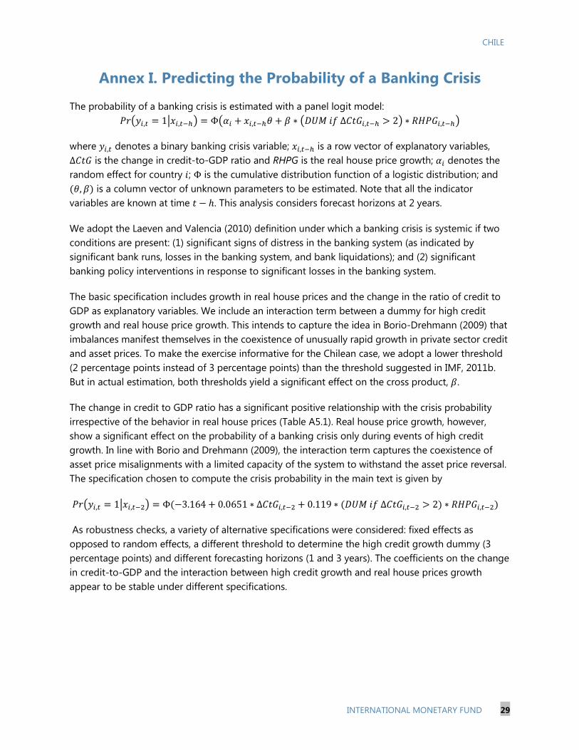
The probability of a banking crisis is estimated with a panel logit model: 𝑃𝑟�𝑦𝑖,𝑡 = 1�𝑥𝑖,𝑡−ℎ� = Φ�𝛼𝑖 + 𝑥𝑖,𝑡−ℎ𝜃 + 𝛽 ∗ �𝐷𝑈𝑀 𝑖𝑓 ∆𝐶𝑡𝐺𝑖,𝑡−ℎ > 2� ∗ 𝑅𝐻𝑃𝐺𝑖,𝑡−ℎ�

where 𝑦𝑖,𝑡 denotes a binary banking crisis variable; 𝑥𝑖,𝑡−ℎ is a row vector of explanatory variables, ∆𝐶𝑡𝐺 is the change in credit-to-GDP ratio and RHPG is the real house price growth; 𝛼𝑖 denotes the random effect for country 𝑖; Φ is the cumulative distribution function of a logistic distribution; and (𝜃,𝛽) is a column vector of unknown parameters to be estimated. Note that all the indicator variables are known at time 𝑡 − ℎ. This analysis considers forecast horizons at 2 years.

We adopt the Laeven and Valencia (2010) definition under which a banking crisis is systemic if two conditions are present: (1) significant signs of distress in the banking system (as indicated by significant bank runs, losses in the banking system, and bank liquidations); and (2) significant banking policy interventions in response to significant losses in the banking system.

The basic specification includes growth in real house prices and the change in the ratio of credit to GDP as explanatory variables. We include an interaction term between a dummy for high credit growth and real house price growth. This intends to capture the idea in Borio-Drehmann (2009) that imbalances manifest themselves in the coexistence of unusually rapid growth in private sector credit and asset prices. To make the exercise informative for the Chilean case, we adopt a lower threshold (2 percentage points instead of 3 percentage points) than the threshold suggested in IMF, 2011b. But in actual estimation, both thresholds yield a significant effect on the cross product, 𝛽.

The change in credit to GDP ratio has a significant positive relationship with the crisis probability irrespective of the behavior in real house prices (Table A5.1). Real house price growth, however, show a significant effect on the probability of a banking crisis only during events of high credit growth. In line with Borio and Drehmann (2009), the interaction term captures the coexistence of asset price misalignments with a limited capacity of the system to withstand the asset price reversal. The specification chosen to compute the crisis probability in the main text is given by

𝑃𝑟�𝑦𝑖,𝑡 = 1�𝑥𝑖,𝑡−2� = Φ(−3.164 + 0.0651 ∗ ∆𝐶𝑡𝐺𝑖,𝑡−2 + 0.119 ∗ (𝐷𝑈𝑀 𝑖𝑓 ∆𝐶𝑡𝐺𝑖,𝑡−2 > 2) ∗ 𝑅𝐻𝑃𝐺𝑖,𝑡−2)

As robustness checks, a variety of alternative specifications were considered: fixed effects as opposed to random effects, a different threshold to determine the high credit growth dummy (3 percentage points) and different forecasting horizons (1 and 3 years). The coefficients on the change in credit-to-GDP and the interaction between high credit growth and real house prices growth appear to be stable under different specifications.

CHILE


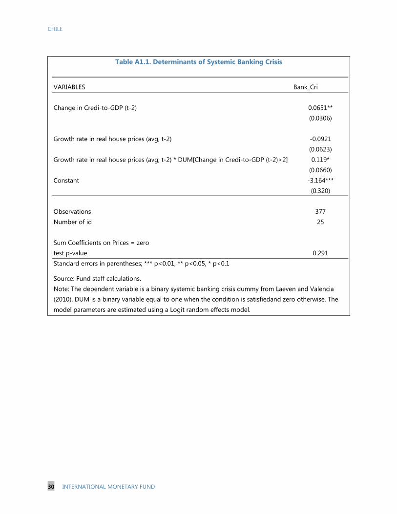
Table A1.1. Determinants of Systemic Banking Crisis

VARIABLES Bank_Cri

Change in Credi-to-GDP (t-2) 0.0651**(0.0306)

Growth rate in real house prices (avg, t-2) -0.0921(0.0623)

Growth rate in real house prices (avg, t-2) * DUM[Change in Credi-to-GDP (t-2)>2] 0.119*(0.0660)

Constant -3.164***(0.320)

Observations 377Number of id 25

Sum Coefficients on Prices = zero test p-value 0.291Standard errors in parentheses; *** p<0.01, ** p<0.05, * p<0.1

Source: Fund staff calculations.Note: The dependent variable is a binary systemic banking crisis dummy from Laeven and Valencia(2010). DUM is a binary variable equal to one when the condition is satisfiedand zero otherwise. The model parameters are estimated using a Logit random effects model.

Annex II. Banking Prudential Toolkit and Governance Table A2.1 Banking Prudential Toolkit and Governance

Readily Available for Active Calibration/Macroprudential Tools Chilean Banking Sector Ownership* Established By Macroprudential Use?

A. LeverageCapital ratio According to Basel I guidelines. Minimum capital ratio of 8%. Adjusted BCCh/SBIF GBA and BCCh norm (III.B.2) Requirements for market risk can be modified

for exposures to market risk. by CBCh; capital ratio is fixed by GBA.

Risk weights Basel I RWs. For mortgages exposures higher RW 60% vs 50% SBIF GBA Yes. GBA allows SBIF to move RWs up to one notch with CBCh authorization.

Provisioning Voluntary additional provisions SBIF SBIF norm Yes

Profit distribution restrictions No restrictions beyond satisfying CAR SBIF GBA No

Credit growthCaps on credit growth No caps # NoCaps on LTV Mortgages exposures:

80% LTV on endorsable mortgage loans SBIF SBIF norm Yes75% LTV on mortgage bills BCCh BCCh norm Yes80% LTV on mortgage loans financed with "mortgage bonds" BCCh BCCh norm YesNo LTV on non-endorsable mortgage loans SBIF SBIF norm Yes.

Other exposures: not in place # NoCaps on DTI 25% Dividend-to-income cap on mortgage bills loans up to UF3000 BCCh BCCh norm Yes

25% Dividend-to-income cap on mortgage loans financed with "mortgage bonBCCh BCCh norm YesGross leverage ratio Minimum core capital to total assets of 3% SBIF GBA No

B. LiquidityLiquidity requirements Sum of mismatches up to 30 days cannot exceed core capital. BCCh BCCh norm (III.B.2) Yes

Sum of mismatches up to 90 days cannot exceed two times core capital. BCCh BCCh norm (III.B.2) Yes

Reserve requirements Reserve requirements : sigh deposits 9%, time deposits 3.6%. BCCh BCCh norm (Cap. 3.1) YesTechnical reserve: sigh deposits that exceed 2.5 times the net worth BCCh GBA Nomust be maintained in cash or in a technical reserve consisting ofdeposits with the CB.

Currency mismatch/open FX position limitNet FX flows up to 30 days cannot exceed core capital and built in to Market RBCCh BCCh norm (III.B.2) Yes

C. InterconnectednessConcentration limits Limits on interbank (established in Chile) loans: may not exceed 30% of SBIF GBA No

bank's creditor capital.

BCCh BCCh norm (III.B.2) Yes

Total lending to related parties (including parents) are limited to SBIF GBA No25 percent of capital (secured) or 5 percent of capital (unsecured).

Concentration limits by economic sector No limits. # No

Systemic capital surcharge Capital surcharges for systemically important entities. Capital ratio up SBIF GBA and BCCh norm (III.B.2) Only for M&A that result in significantto 14 percent. Technical reserve if deposits exceed 1.5 times its core market share. capital. Limit on interbank exposure up to 20% of capital.

* Ownership is defined as the institution that could issue regulation calibrating the instrument (but not relaxing beyond GBA when corresponding).GBA: General Banking Act; BCCh: Central Bank of Chile; SBIF: Superintendence of Banks and Financial Institutions; M&A: Merger and Acquisitions; Monetary Unit (UF) Unidad de Fomento.# Legal changes would be necessary to assign ownership to regulate this as well as to assign ownership to regulators.

Limits on (short-term) obligations with banks: short term obligations with one bank cannot exceed 5% of debtor's current assets (individual limit). The sum of short term obligations with all domestic banks cannot exceed 40% of debtor's current assets (global limit).

CHILE

INTERN

ATION

AL MO

NETARY FU

ND

31

CHILE


References

Ahuja, Ashvin and Malhar Naber, “Safeguarding Banks and Containing Property BoomsL Cross-Country Evidence on Macroprudential Policies and Lessons from Hong Kong SAR”, IMF Working Papers, WP/11/284

Almeida, Heitor, Liu, Crocker H. and Campello, Murillo, 2005, “The Financial Accelerator: Evidence

from International Housing Markets.” Available at SSRN: http://ssrn.com/abstract=348740. Arregui, Nicolas, Jaromir Benes, Ivo Krznar, Srobona Mitra, and Andre Oliveira Santos, 2013,

“Evaluating the Net Benefits of Macroprudential Policy: A Cookbook”, forthcoming (Washington: International Monetary Fund).

Barrell, Ray, E Philip Davis, Dilruba Karim and Iana Liadze, 2010, “Bank regulation, property prices

and early warning systems for banking crises in OECD countries,” Journal of Banking and Finance, Vol. 34, pp. 2255-2264.

Berger, Allen N., and Gregory F. Udell, 2004, “The Institutional Memory Hypothesis and the

Procyclicality of Bank Lending Behavior,” Journal of Financial Intermediation, Vol. 13, pp. 458–95.

Borio, C. and P. Lowe, 2002, “Assessing the risk of banking crises,” BIS Quarterly Review, December, 43–54. _______, and M. Drehmann, 2009, “Assessing the risk of banking crises – revisited,” BIS Quarterly Review, March, 29–46. Chan-Lau, J.A., 2009, “The Global Financial Turmoil and Its Impact on Chilean Banks,” IMF Country

Reports 09/272 (Washington: International Monetary Fund). __________, 2010, “Too Connected to Fail Risk in the Chilean Banking System: a Balance Sheet

Network Analysis,” IMF Country Reports 10/299 (Washington: International Monetary Fund). __________, 2012, “Do Dynamic Provisions Enhance Bank Solvency and Reduce Credit Procyclicality?

A Study of the Chilean Banking System,” IMF Working Papers WP/12/124 (Washington: International Monetary Fund).

Committee on the Global Financial System, 2012, “Operationalising the Selection and Application of

Macroprudential Instruments,” CGFS Papers No. 48. Dell’Ariccia, Giovanni, Deniz Igan, Luc Laeven, and Hui Tong, 2012,“Policies for Macrofinancial

Stability: Options to Deal with Credit Booms,” IMF Staff Discussion Note SDN/12/06 (Washington: International Monetary Fund).

CHILE


Dell’Ariccia, Giovanni, and Robert Marquez, 2006, “Lending Booms and Lending Standards,” Journal of Finance, Vol. 61, No. 5, pp. 2511–546.

De Nicolò, Gianni, Giovanni Favara, and Lev Ratnovski, 2012, “Externalities and Macroprudential

Policy,” IMF Staff Discussion Note, SND/12/05 (Washington: International Monetary Fund). International Monetary Fund, 2008, “Financial Stress and Economic Downturns” World Economic

Outlook, World Economic and Financial Surveys (Washington; October). _____, 2011a, “Macroprudential Policy: An Organizing Framework” IMF Policy Papers (Washington;

March). _____, 2011b, “Toward Operationalizing Macroprudential Policies: When to Act?” Global Financial

Stability Report, World Economic and Financial Surveys (Washington; September). _____, 2011c, “Macroprudential Policy: What Instruments and How to use them? Lessons from

Country Experiences,” IMF Working Papers 11/238 (Washington; September). _____, 2012a, “Republic of Poland: Technical Assistance Report—Macroprudential Framework” IMF

Country Reports 12/276 (Washington: International Monetary Fund). _____, forthcoming, “Key Aspects of Macroprudential Policy” (Washington: International Monetary

Fund). Illing, Mark and Liu, Ying, 2006. "Measuring financial stress in a developed country: An application

to Canada," Journal of Financial Stability, Elsevier, vol. 2(3), pages 243– 65 (October). Jorda, Oscar, Moritz Schularick and Alan Taylor, 2011. "Financial Crises, Credit Booms, and External

Imbalances: 140 Years of Lessons," IMF Economic Review, Palgrave Macmillan, vol. 59(2), pages 340–378 (June). Kaminsky, Graciela, and Carmen Reinhart, 1999, “The Twin Crises: The Causes of Banking and

Balance-of-Payments Problems,” American Economic Review, Vol. 89, pp. 473 500. Kuttner, K and I Shim (2012): “Taming the real estate beast”, mimeo. Laeven, Luc, and Fabian Valencia, 2010, “Resolution of Banking Crises: The Good, the Bad, and the

Ugly,” IMF Working Papers 10/146 (Washington: International Monetary Fund). Lim, Cheng-Hoon, F. Columba, A. Costa, P. Kongsamut, A. Otani, M. Saiyid, T. Wezel, and X. Wu,

2011, “Macroprudential Policy: What Instruments and How to Use Them, Lessons from Country Experiences,” IMF Working Papers 11/238 (Washington: International Monetary Fund).

CHILE


Lund-Jensen, Kasper, 2012, “Monitoring Systemic Risk Using Dynamic Thresholds,” IMF Working

Papers 12/159, (Washington: International Monetary Fund). Mendoza, Enrique G., and Marco E. Terrones, 2008, "An Anatomy Of Credit Booms: Evidence From

Macro Aggregates And Micro Data," NBER Working Papers 14049, National Bureau of Economic Research, Inc.

Rajan, Raghuram G., 1994, “Why Bank Credit Policies Fluctuate: A Theory and Some Evidence,”

Quarterly Journal of Economics, Vol. 109, No. 2, pp. 399–441. Rancière, Romain, Aaron Tornell, and Frank Westermann, 2008, “Systemic Crises and Growth,”

Quarterly Journal of Economics, Vol. 123, No. 1, pp. 359–406. Reinhart, C., and K. Rogoff, 2009, “This Time is Different: Eight Centuries of Financial Folly,”

(Princeton, New Jersey: Princeton University Press). Ruckes, Martin, 2004, “Bank Competition and Credit Standards,” Review of Financial Studies, Vol. 17,

No. 4, pp. 1073-102. Shin, Hyun Song and Shin, Kwanho, 2011, “Procyclicality and Monetary Aggregates,” No 16836,

NBER Working Papers, National Bureau of Economic Research, Inc. Vandenbussche, J., U. Vogel, and E. Detragiache, 2012. "Macroprudential Policies and Housing

Prices-A New Database and Empirical Evidence for Central, Eastern, and Southeastern Europe," IMF Working Papers 12/303, International Monetary Fund.

Wong, T. C., Fong, Tom, Li, Ka-Fai and Choi, Henry, 2011, “Loan-to-Value Ratio as a Macroprudential

Tool - Hong Kong's Experience and Cross-Country Evidence.” Available at SSRN: http://ssrn.com/abstract=1768546.

CHILE


WHAT EXPLAINS MOVEMENTS IN THE PESO/DOLLAR EXCHANGE RATE?1

This chapter examines the factors affecting the peso exchange rate. While copper price is the most important determinant over the long run, other factors including interest rate differential, global financial distress, local pension funds’ derivative position, as well as the Federal Reserve’s quantitative easing also affect the peso in the short run.

A. Introduction

1. The Chilean peso has historically moved closely with copper prices. In 2012, copper accounted for 54 percent of Chile’s exports, 14 percent of fiscal revenue, and 13 percent of nominal GDP. The Chilean peso is one of the so-called “commodity currencies.” While it is notoriously difficult to explain short-term exchange rate movements, the literature has established commodity prices as a robust and exogenous fundamental in explaining the behavior of the commodity currencies (Amano and van Norden, 1993; Cashin, Cespedes, and Sahay, 2004).

2. There are, however, episodes when the peso deviates from copper prices (Figure 1). One such episode began on June 2012: the peso appreciated almost 6 percent against the U.S. dollar (as of May 24) despite a small decline in copper prices. Notwithstanding the recent weakening of the peso (which is also a regional phenomenon), it still appears to be stronger than justified by copper prices. This raises the question what other factors also drive peso’s movements. For example, there have been much public debate in Chile on the influence on the peso from monetary policy in advanced economies and capital flows (Larraín, 2013).

3. This chapter seeks to explain the peso movements, using a simple error-correction model. The study uses weekly dollar/peso exchange rate data from October 1, 1999, when the peso became floating, to May 24, 2013. Weekly data are used because some explanatory variables are only available on weekly basis and because it helps smooth the noisy daily exchange movements. The focus on the nominal exchange rate is because it is available at high frequency.

4. A number of past research examined the peso exchange rate. Cowan, Rappoport, and Selaive (2007) studied the determinants of peso-dollar exchange rate using daily data from 1993 to 2006. They found that copper and oil prices are important determinants of the long and short term dynamics of the peso, and changes in the pension funds’ limits on foreign assets had small and transitory effects. Caputo, Núñez, and Valdés (2008) studied the peso real exchange rate using quarterly data. The Chilean peso is also often included in studies on commodity currencies (e.g., Chen and Rogoff, 2003 and 2012).

1 Prepared by Yi Wu. Diego Gianelli G., Philip Liu, Li Zeng, and seminar participants at the Central Bank of Chile provided very helpful comments and suggestions. Matias Arnal helped with data collection.

CHILE


5. Our model fits the in-sample exchange rate movements well, including for the recent period. It finds that while copper price is the most important driver of peso exchange rate, accounting for the bulk of its long-run movements, other factors including interest rate differential, global financial distress, the Federal Reserve’s quantitative easing (QE), and local pension funds’ foreign exchange derivative position also affect the peso exchange rate in the short run. The strength of the peso since last June seems to be attributable to combination of factors, including the moderation in global financial risks and the QE.

6. This chapter is organized as follows: Section B discusses possible determinants of the peso exchange rate; Section C discusses the framework and data for the empirical test; Section D presents the statistical results; and Section E provides some concluding remarks.

B. Possible Determinants of the Peso Exchange Rate

7. Strong capital inflows seem to have helped support peso. FDI and portfolio inflows, both gross and net, have increased substantially after the 2008/09 global financial crisis (Figure 2), along with a generally strengthening peso. Gross inflows reached historical high in 2012 with record FDI and portfolio inflows. While capital outflows also increased substantially in 2012 (in particular outward investment by Chilean pension funds, leading to decline in net inflows), net capital inflows improved sharply in the second half of the year, coinciding with the strengthening of the peso. It should also be noted that copper prices could affect capital inflows indirectly, e.g., through its impact on domestic demand.

8. Carry trade, one form of capital flows, may also have affected the peso. The main form of carry trade for nonresidents is through the foreign exchange forward market (Chan-Lau, 2009).2 These activities have been particularly volatile in recent months (see more in the next paragraph). Investors would use dollar (which has a lower interest rate) as the funding currency to invest in the peso, where they just hold a long peso position in the forward market, which would lead to a strengthening of the peso in the sport market.3

2 This is partially due to barriers for nonresidents to enter the local bond market. For example, registering to buy bonds in Chile takes about six months (Bloomberg, 2013).

Chile’s onshore forward market is deep with daily transactions averaging $3 billion. Transactions include both deliverable and non-deliverable forward, but the latter is more common. Average daily turnover at the offshore forward market (non-deliverable only) amounts to $0.5-$1 billion (HSBC, 2013). Chile’s onshore spot market is one of Latin America’s most liquid, with an average daily turnover of US$1.8-2.3 billion, and spot transactions can only be done onshore. Investors have also used the peso as the funding currency to invest in the Brazilian real (as interest rates are lower in Chile). In such a case, they would hold a short position in the peso in the forward market,

3 Domestic banks are the counterparty to these long peso positions in the onshore market, and they would sell dollar in the spot market to balance it, strengthening the peso in the spot market.

CHILE


which would weaken the peso in the spot market.4

9. Carry trade seems to contribute to the peso’s weakening since May. While carry traders using dollar as the funding currency would hold a short dollar position, nonresidents as a whole usually hold a net long position in dollar, suggesting that many positions are probably for real hedging needs. However, between November 2012 and February 2013, nonresidents have substantially reduced their long dollar position (by $7.7 billion in the on-shore market, Figure 3a). This is consistent with an increase in carry trade with the peso as the target currency. By November the peso had already appreciated significantly and the subsequent appreciation was moderate. It therefore seems that the impact of carry trade on the peso’s strength before May was probably moderate and “carry traders” were mostly “chasing” the peso’s appreciation.

But compared with carry traders using dollar as the funding currency, the former group appears to be dominant, at least in the recent period.

5

10. Our model controls for interest differentials for the short-run peso dynamics, as the standard practice in the literature, instead of directly controlling for capital flows. There are no direct data on carry trade, and capital flows data are only available on a monthly basis. In addition, estimates directly using capital flows could be more subject to the endogeneity problem. Some factors could by themselves lead to an appreciation of the peso and increased capital inflows, and there could be an endogeneity problem if these factors are not properly accounted for. Capital flows could also be endogenously responding to exchange rate movements. Interest differential is more likely to be exogenous: with the implementation of a full-fledged inflation targeting regime and a floating exchange rate in 1999, Chile’s monetary policy has been mostly responding to inflation (and business cycles), instead of to exchange rate movements (Central Bank of Chile, 2007; McGettigan et al., 2013).

Nonresidents subsequently dramatically reversed their positions, and their net long dollar positions reached $13.2 billion by early June (up from $2.7 billion in mid-April)−the highest since October 2008, when the data first became available. This reversal seems to have contributed to the peso’s deprecation since May.

11. Local institution investors also play an important role in determining the peso exchange rate. This is particularly the case for pension funds. Assets under management of Chilean pension funds amounted to $162 billion at end-2012 (60 percent of GDP), with pension funds’ oversea investment standing at $62 billion. Movements of these assets can have a large impact on local capital markets and interest rate, as well as on the exchange rate. As required by Chilean regulations, pension funds need to hedge part of their oversea investments via holding short dollar positions (about US$10.4 billion as of end-March 2013) in the onshore derivative market.6

4 These investors would hold simultaneous short peso positions vs. dollar and long positions in Brazilian real vs. dollar.

As the hedging is required by

5 This could be a self-enforcing circle: the peso’s appreciation may attract more long peso positions in the forward market, which would strengthen the peso in the spot market further. Granger causality tests do suggest that nonresidents’ forward position and the peso exchange rate have predicting power over each other. 6 Pension funds’ net short dollar positions in the off-shore market were much smaller, at $54 million at the same time. Ideally pension funds’ net transactions in the spot market should also be controlled for, but these are not published (and relatively small).

CHILE


regulation (there are also episodes of regulation changes), it can be considered largely exogenous. The data for pension funds’ derivative position are only available from 2007 onward, it is therefore only included in the robustness checks.

12. The model also accounts for other factors that may affect the peso including Federal Reserve’s quantitative easing (QE) and global financial distress. The QE (November 2008–March 2010, November 2010–July 2011, and since September, 2012) could affect the dollar/peso exchange rate by affecting the interest rate differential (although the U.S. short-term interest rate has been close to zero since late 2008). They could also have impact on commodity prices, including copper. On top of these channels, the size of the Federal Reserve’s balance sheet could have additional impact on the peso exchange rates, e.g., through capital flows and expectations. Our estimations therefore include the balance sheet size of the Federal Reserve and the Central Bank of Chile for the analysis of the short-run dynamics of the exchange rate. The model also includes measures of global and local risks. Finally, since expectations play an important role in exchange rate movements (Dornbusch, 1976), 7

13. We also conduct some simple analysis on the short-run effect of the two latest foreign exchange interventions by the Central Bank of Chile. We use dummy variables to capture the Central Bank’s interventions in 2008 and 2011, when it conducted $50 million daily dollar purchases in the spot market in both cases (fully sterilized). Studies of Chile’s earlier intervention episodes (August 16, 2001–January 1, 2002 and October 10, 2002–February 10, 2003, where the Central Bank sold dollars) found that the most important impact of intervention came from the announcement (De Gregorio and Tokman, 2004; Cowan, Rappoport, and Selaive, 2007). This also seems to be the case in 2011, when the peso weakened by 4½ percent against the U.S. dollar the day after the announcement, and depreciated 6½ percent in the first week (the peso subsequently quickly recovered). A simple dummy variable for the intervention won’t be able to capture all the dynamics, but it would capture the average impact of the invention−while it is in place.

we also include expected future GDP growth in the robustness checks (the data are only available from 2007).

C. The Analytical Framework and Data

14. We use an error-correction model that is similar to what is used in other studies that addresses both the long-run and short-run dynamics of the exchange rate (e.g., Cowan, Rappoport, and Selaive, 2007; Helliwell et al., 2004; Moazzami and Anderson, 2003).

Long-run dynamics EXt = α0+ α1Coppert + α1Oilt + α3Rel-CPIt + et, (1)

7 Which is the reason that Chen, Rogoff, and Rossi (2010) find that commodity currency exchange rates have robust power in predicting global commodity prices, since they already incorporate expectations of future commodity prices.

CHILE


where EXt is the logarithm of the nominal dollar/peso exchange rate, at end-week. All explanatory variables are weekly averages to help reduce endogeneity. The estimates basically capture the contemporaneous effects. Copper denotes the logarithm of copper prices and Oil denotes the logarithm of oil prices. Chile is a net oil importer, 8

Short-run dynamics

and higher oil prices would lead to a deterioration of the terms of trade and thus a likely weakening of the peso. Rel-CPI represents the ratio of U.S. CPI index to that of Chile. Monthly CPI index is converted into weekly index by interpolation. et denotes the error term.

∆EXt = β0 + β1∆Coppert + β2∆Rel-CPIt + β3∆CHL-USt + β4∆BRA-CHLt + β5∆CDS-Chilet + β6∆ESP-DEUt +

β7∆VIXt + β8∆FEDt-9 + β9∆BCCht-9 + β10∆Rel-stockt-9 + β11∆Interve2008t + β12∆Interve2011t

+ β13ECt-1+εt, (2)

∆ denotes the first deference. The oil price is not included in the short-run specification because it turns out to be insignificant in the long-run specification as discussed below. CHL-US is the interest spread between the 90-day Chile and U.S. government bills−the 90-day government bill market is the most liquid in Chile. A higher spread is expected to attract more portfolio and carry trade inflows to Chile, and lead to a stronger peso. BRA-CHL is the difference of the 90-day Brazilian and Chilean government bill yields. This serves as a proxy for alternative investment opportunities for international investors in the region (or among emerging markets), or carry trade opportunities using peso as the funding currency. In both cases, a higher Brazil-Chile interest spread is expected to weaken the peso.

CDS-Chile represents 5-year sovereign credit default swap spread (CDS) for Chile. It measures the perceived risks of investing in Chilean securities. ESP-DEU is the interest spread between 10-year Spanish and German government bonds. It serves as a proxy for financial distress in Europe. VIX is the implied volatility of S&P 500 index options, a common measure of global financial distress.

FED denotes the balance sheet size of the U.S. Federal Reserve (base money) in trillions of dollars. This would capture the impact of the QE on the peso exchange rate in additional to its impact through reducing U.S. interest rates. Unlike the case of interest differential, currency movements in response to monetary expansion need not be instantaneous, and may take place over a more prolonged period (Ghosh and Qureshi, 2013). We therefore used a two-month lag for the Fed’s balance sheet. BCCh denotes the balance sheet size of the Central Bank of Chile in trillions of pesos, also in 2-month lag. The data for BCCh are published for every eight days, which are converted into weekly data by interpolation.

Rel-stock is the ratio of Santiago stock exchange’s IPSA index to the U.S. S&P 500 index. Higher stock market returns are expected to lead to more portfolio inflows. Again a 2-month lag is used. Interve2008 and Interve2011 are dummies for the foreign exchange interventions by the Central Bank

8 Oil imports accounted for 8 percent of total imports in 2012.

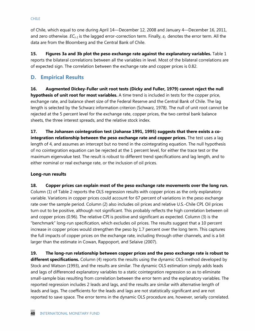
CHILE


of Chile, which equal to one during April 14—December 12, 2008 and January 4—December 16, 2011, and zero otherwise. ECt-1 is the lagged error-correction term. Finally, εt denotes the error term. All the data are from the Bloomberg and the Central Bank of Chile.

15. Figures 3a and 3b plot the peso exchange rate against the explanatory variables. Table 1 reports the bilateral correlations between all the variables in level. Most of the bilateral correlations are of expected sign. The correlation between the exchange rate and copper prices is 0.82.

D. Empirical Results

16. Augmented Dickey-Fuller unit root tests (Dicky and Fuller, 1979) cannot reject the null hypothesis of unit root for most variables. A time trend is included in tests for the copper price, exchange rate, and balance sheet size of the Federal Reserve and the Central Bank of Chile. The lag length is selected by the Schwarz information criterion (Schwarz, 1978). The null of unit root cannot be rejected at the 5 percent level for the exchange rate, copper prices, the two central bank balance sheets, the three interest spreads, and the relative stock index.

17. The Johansen cointegration test (Johanse 1991, 1995) suggests that there exists a co-integration relationship between the peso exchange rate and copper prices. The test uses a lag length of 4, and assumes an intercept but no trend in the cointegrating equation. The null hypothesis of no cointegration equation can be rejected at the 1 percent level, for either the trace test or the maximum eigenvalue test. The result is robust to different trend specifications and lag length, and to either nominal or real exchange rate, or the inclusion of oil prices.

Long-run results

18. Copper prices can explain most of the peso exchange rate movements over the long run. Column (1) of Table 2 reports the OLS regression results with copper prices as the only explanatory variable. Variations in copper prices could account for 67 percent of variations in the peso exchange rate over the sample period. Column (2) also includes oil prices and relative U.S.-Chile CPI. Oil prices turn out to be positive, although not significant. This probably reflects the high correlation between oil and copper prices (0.96). The relative CPI is positive and significant as expected. Column (3) is the “benchmark” long-run specification, which excludes oil prices. The results suggest that a 10 percent increase in copper prices would strengthen the peso by 1.7 percent over the long term. This captures the full impacts of copper prices on the exchange rate, including through other channels, and is a bit larger than the estimate in Cowan, Rappoport, and Selaive (2007).

19. The long-run relationship between copper prices and the peso exchange rate is robust to different specifications. Column (4) reports the results using the dynamic OLS method developed by Stock and Watson (1993), and the results are similar. The dynamic OLS estimation simply adds leads and lags of differenced explanatory variables to a static cointegration regression so as to eliminate small-sample bias resulting from correlation between the error term and the explanatory variables. The reported regression includes 2 leads and lags, and the results are similar with alternative length of leads and lags. The coefficients for the leads and lags are not statistically significant and are not reported to save space. The error terms in the dynamic OLS procedure are, however, serially correlated.

CHILE


The standard errors are therefore estimated using the Newey and West (1987) adjustment with a lag length of up to 2. Column (5) reports the results using log real peso exchange rate (essentially imposing a unit coefficient on the relative CPI), where the coefficient for copper prices is slight larger. Column (6) reports the results for the sample ending at end-2011. Compared with the results reported in Column (3), the coefficient on copper prices is very close, while the coefficient for the error-correction term is a bit larger.

Short-run results

20. Some other explanatory variables are also important in the short run. Column (1) of Table 3a reports the short-run results including all explanatory variables, where the sample size is reduced to 2003 onward. Column (2) then only includes the significant variables: the Chile-U.S. interest differential, VIX, the central bank balance sheets, and the intervention dummies. The data are also available for the whole sample period. We also tried to include one lag of the explanatory variables and the results are reported in Column (3). The lagged variables are insignificant (not reported to save space) except for copper prices. Column (4) of Table 3a reports the results using the real peso-dollar exchange rate as the dependent variable. The results (for the significant variables) are broadly similar across Columns (1) to (4). All short-run regressions are based on corresponding long-run results reported in Table 2.

21. The coefficient on the Chile-U.S. short-term interest is small, while the coefficient on VIX is relatively large. A 100 basis points (bps) increase in the spread would only strengthen the peso by 0.4 percent against the dollar in the short run, using the results form Column (2), which is our benchmark short-run specification.9

22. A larger balance sheet of the Federal Reserve is associated with a peso appreciation against the dollar in the short run. The Federal Reserve’s balance sheet has increased by about $450 billion since September 2012 when QE3 was introduced. The regression results suggest that this expansion would imply a strengthening of the peso by about 2 percent (although there will be a lag for the full impact). The expansion of the Federal Reserve’s balance sheet during the height of the 2008/09 financial crisis and the subsequent QE (in particular QE2 and QE3) may be of different nature. To control for this possibility, we also added the interaction of the Fed’s balance sheet and a dummy variable which equals to 1 after the implementation of QE1 or QE2. This term turns out to be insignificant in either case, while other results remain unchanged (results not reported).

Higher global financial distress, as measured by VIX, would weaken the peso, and the impact is relatively large: a one standard deviation increase in VIX (about 9) would weaken the peso by about 2 percent. The VIX has declined by 12 points between June 2012 and mid-March 2013, and subsequently rose 2 points.

9 Level regression would yield a substantially larger coefficient. The Chile-U.S. interest differential is of the “wrong” sign in Cowan, Rappoport, and Selaive (2007).

CHILE


23. In contrast, a larger balance sheet of the Central Bank of Chile would weaken the peso in the short run, everything else equal. In addition, the Central Bank’s interventions in 2008 and 2011 seem to have a moderate impact on the exchange rate in the short run. The estimates suggest that the peso has been weakened by about 3½ and 2½ percent, by the two interventions, respectively. Finally, the other explanatory variables included in Column (1) are insignificant.10

In-sample forecasts

24. The model fits the in-sample peso exchange rate movements reasonably well. Figure 4 plots the actual dollar/peso exchange rate (in log) vs. the 3-month dynamic simulation forecast, using the coefficients from Column (3) of Table 2 and Colum (2) of Table 3a. The model’s projections are based on dynamic simulations of equations (1) and (2), so the projected value at time t is used to calculate the prediction at t+1, etc., over the next 3 months on a rolling basis. The forecast tracks the actual peso movements relatively well, including for the recent period. The forecast stops at April 2013 since the relative CPI data are only available up to April. Finally, Colum (4) of Table 3a reports the results using the real dollar/peso exchange rate as the dependent variable. The results are very close to those of Column (2).

25. Forecasting using a shorter sample period yield very similar results. Column (1) of Table 2b reports the results for the sub-sample ending in 2011. The result is pretty close to the baseline results, although the coefficient for the balance sheet of Central Bank of Chile becomes statistically insignificant. 3-month dynamic simulation forecast yield almost identical results as those shown in Figure 4.

Adding additional explanatory variables

26. We next add three additional explanatory variables to the short-run equation:

U.S. nominal effective exchange rate. This variable is added to control for the possibility that the movements in the dollar/peso exchange rate simply reflects a U.S. dollar story. The data are only available on monthly basis (and up to March) and are converted into weekly data by interpolation.

Pension funds’ short dollar forward position. This is the short forward dollar position held by the Chilean pension funds in the local foreign derivative market, in billions of dollars. The Central Bank publishes monthly data for 2007-08 and four observations each month since 2009. These are converted into weekly data by interpolation.

Expected growth over the next 12 months. A better growth perspective is expected to lead to a stronger peso. The Central Bank publishes monthly survey to local economists on expected annual growth rate for the current and the next year. The expected growth over the next 12 months is derived, as a proxy,

10We also used the average CDS of European banks to replace Spain-Germany spread as the measures of financial distress in Europe, which is also insignificant.

CHILE


as the weighted average of the expected growth for the current and the next year, using the remaining months of the current year as the weight for the current year. The monthly data are then converted into weekly data by interpolation.

27. The results are broadly similar with the baseline results for the original variables. Column (1) of Table 3b reports the results including the U.S. nominal effective exchange rate as the additional explanatory variable. The U.S. nominal exchange rate is negative and significant as expected, while the coefficients for other variables are broadly similar to the benchmark specification, except that the relative CPI becomes statistically insignificant. Column (2) of Table 3b reports the results adding the pension’s short dollar position and the expected GDP growth, where the sample size is substantially smaller. The pension’s short dollar position is positive as expected and significant at the 1 percent level. The estimate suggests that an increase of local pension funds’ short dollar position by $1 billion would strengthen the peso by 0.4 percent against the dollar. The growth expectation turns out to be negative (although insignificant), even though it has a high positive simple correlation with the peso exchange rate (0.63). This may reflect the fact that the expected growth is highly correlated with copper prices (correlation 0.78) which is already included in the regression. The coefficients for other variables are broadly similar to the benchmark specification, except that the coefficient for the error correction term is a bit larger, and the Chile-U.S. interest rate spread becomes insignificant (p-value is 0.13).

E. Summary

28. This chapter examines the weekly nominal dollar/peso exchange rate between October 1999 and May 2013 using an error-correction model. The model fits the historical exchange rate well. While copper prices can explain the bulk of peso movements over the long run, other factors also play important role in the short run, including interest differential, global financial risks and local pension funds’ foreign exchange derivative position. The QE also seems to lead to a strengthening of the peso. The analysis finds that the Central Bank of Chile’s foreign exchange interventions in 2008 and 2011 had a small impact on the peso.

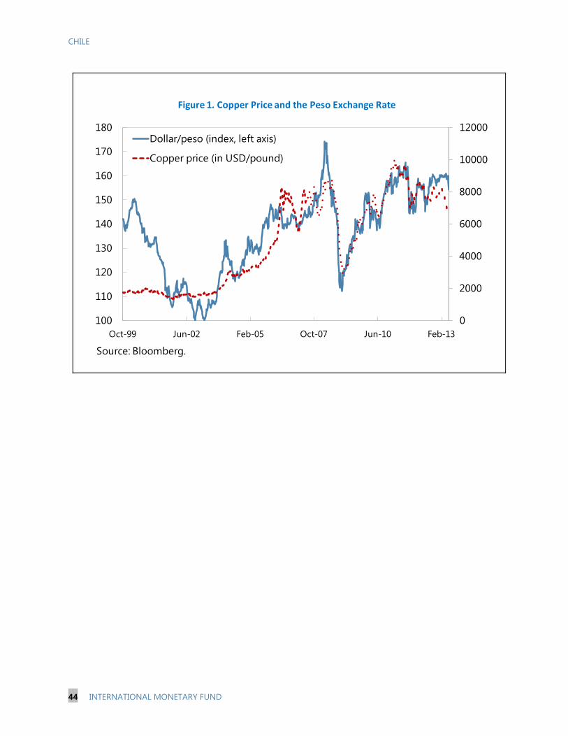
CHILE


0

2000

4000

6000

8000

10000

12000

100

110

120

130

140

150

160

170

180

Oct-99 Jun-02 Feb-05 Oct-07 Jun-10 Feb-13

Dollar/peso (index, left axis)

Copper price (in USD/pound)

Figure 1. Copper Price and the Peso Exchange Rate

Source: Bloomberg.

CHILE


Figure 2. Capital Flows

Source: Central Bank of Chile.

-8

-6

-4

-2

0

2

4

6

8

-8

-6

-4

-2

0

2

4

6

8

Jan-07 Jan-08 Jan-09 Jan-10 Jan-11 Jan-12 Jan-13

NetOutflowsInflows

Financial Account(In billions of U.S. dollars, 3-month moving average)

-5

-4

-3

-2

-1

0

1

2

3

4

5

-5

-4

-3

-2

-1

0

1

2

3

4

5


NetOutflowsInflows

Foreign Direct Investment(In billions of U.S. dollars, 3-month moving average)

-3

-2

-1

0

1

2

3

-3

-2

-1

0

1

2

3


Net

Outflows

Inflows

Portfolio Flows(In billions of U.S. dollars, 3-month moving average)

-4

-3

-2

-1

0

1

2

3

4

-4

-3

-2

-1

0

1

2

3

4


Net

Outflows

Inflows

Other Investments(In billions of U.S. dollars, 3-month moving average)

CHILE


Figure 3a. What Explains Peso Movements

Sources: Bloomberg and Central Bank of Chile.

-4.00

-2.00

0.00

2.00

4.00

6.00

8.00

10.00

12.00

100

110

120

130

140

150

160

170

Oct-08 Apr-10 Oct-11 Apr-13


Long forward position in bil USD by nonresidents

-1

0

1

2

3

4

5

6

7

8

9

100

110

120

130

140

150

160

170

180



Chile-U.S. 90-day interest spread

-1

0

1

2

3

4

5

6

7

100

110

120

130

140

150

160

170

180



Spain-Germany 10-year interest spread

0

0.5

1

1.5

2

2.5

3

100

110

120

130

140

150

160

170

180

Jan-03 Jan-05 Jan-07 Jan-09 Jan-11 Jan-13


CHILE 5-year CDS

0

10

20

30

40

50

60

70

80

100

110

120

130

140

150

160

170

180



VIX


0

0.5

1

1.5

2

2.5

3

3.5

100

110

120

130

140

150

160

170

180


Dollar/peso (index, left axis)FED balance sheet

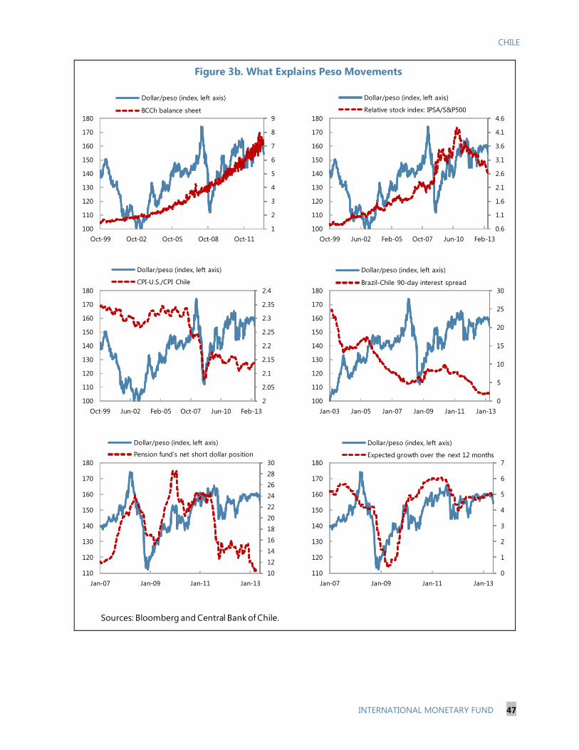
CHILE


Figure 3b. What Explains Peso Movements


1

2

3

4

5

6

7

8

9

100

110

120

130

140

150

160

170

180

Oct-99 Oct-02 Oct-05 Oct-08 Oct-11


BCCh balance sheet

0.6

1.1

1.6

2.1

2.6

3.1

3.6

4.1

4.6

100

110

120

130

140

150

160

170

180



Relative stock index: IPSA/S&P500

2

2.05

2.1

2.15

2.2

2.25

2.3

2.35

2.4

100

110

120

130

140

150

160

170

180



CPI-U.S./CPI Chile

0

5

10

15

20

25

30

100

110

120

130

140

150

160

170

180

Jan-03 Jan-05 Jan-07 Jan-09 Jan-11 Jan-13


Brazil-Chile 90-day interest spread

10

12

14

16

18

20

22

24

26

28

30

110

120

130

140

150

160

170

180

Jan-07 Jan-09 Jan-11 Jan-13


Pension fund's net short dollar position

0

1

2

3

4

5

6

7

110

120

130

140

150

160

170

180

Jan-07 Jan-09 Jan-11 Jan-13


Expected growth over the next 12 months

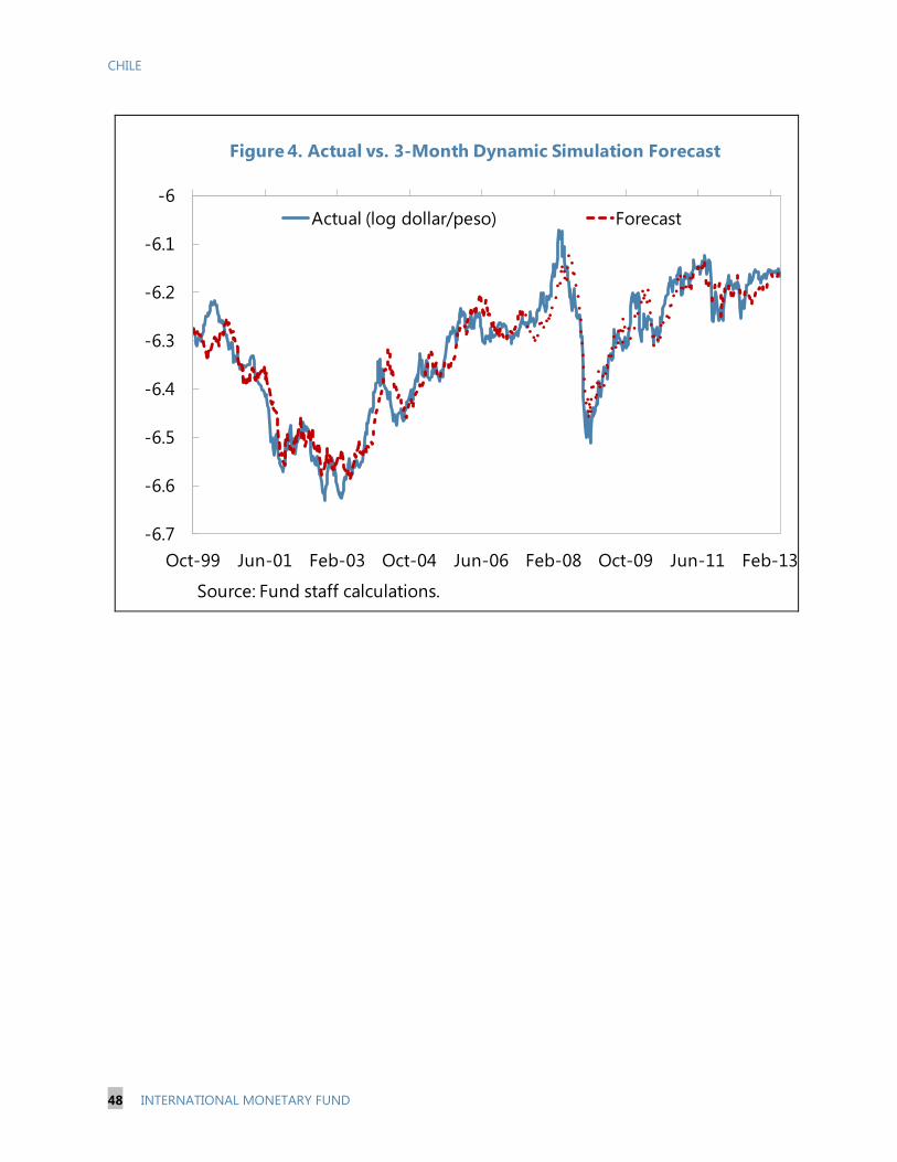
CHILE


-6.7

-6.6

-6.5

-6.4

-6.3

-6.2

-6.1

-6

Oct-99 Jun-01 Feb-03 Oct-04 Jun-06 Feb-08 Oct-09 Jun-11 Feb-13

Actual (log dollar/peso) Forecast

Source: Fund staff calculations.

Figure 4. Actual vs. 3-Month Dynamic Simulation Forecast

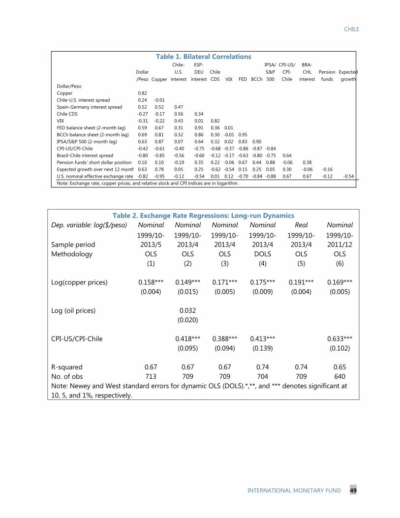
CHILE


Table 1. Bilateral Correlations

Table 2. Exchange Rate Regressions: Long-run Dynamics Dep. variable: log($/peso) Nominal Nominal Nominal Nominal Real Nominal

Sample period 1999/10-2013/5

1999/10-2013/4

1999/10-2013/4

1999/10-2013/4

1999/10-2013/4

1999/10-2011/12

Methodology OLS OLS OLS DOLS OLS OLS

(1) (2) (3) (4) (5) (6)

Log(copper prices) 0.158*** 0.149*** 0.171*** 0.175*** 0.191*** 0.169***

(0.004) (0.015) (0.005) (0.009) (0.004) (0.005)

Log (oil prices)

0.032

(0.020)

CPI-US/CPI-Chile

0.418*** 0.388*** 0.413***

0.633***

(0.095) (0.094) (0.139)

(0.102)

R-squared 0.67 0.67 0.67 0.74 0.74 0.65 No. of obs 713 709 709 704 709 640 Note: Newey and West standard errors for dynamic OLS (DOLS).*,**, and *** denotes significant at 10, 5, and 1%, respectively.

Dollar/Peso Copper

Chile-U.S.

interest

ESP-DEU

interest Chile CDS VIX FED BCCh

IPSA/ S&P 500

CPI-US/ CPI-Chile

BRA-CHL

interest Pension funds

Expected growth

Dollar/PesoCopper 0.82Chile-U.S. interest spread 0.24 -0.01Spain-Germany interest spread 0.52 0.52 0.47Chile CDS -0.27 -0.17 0.56 0.34VIX -0.31 -0.22 0.43 0.01 0.82FED balance sheet (2-month lag) 0.59 0.67 0.31 0.91 0.36 0.01BCCh balance sheet (2-month lag) 0.69 0.81 0.32 0.86 0.30 -0.01 0.95IPSA/S&P 500 (2-month lag) 0.63 0.87 0.07 0.64 0.32 0.02 0.83 0.90CPI-US/CPI-Chile -0.42 -0.61 -0.40 -0.75 -0.68 -0.37 -0.86 -0.87 -0.84Brazil-Chile interest spread -0.80 -0.85 -0.56 -0.60 -0.12 -0.17 -0.63 -0.80 -0.75 0.64Pension funds' short dollar position 0.10 0.10 -0.19 0.35 0.22 -0.06 0.67 0.44 0.88 -0.06 0.38Expected growth over next 12 month 0.63 0.78 0.05 0.25 -0.62 -0.54 0.15 0.25 0.05 0.30 -0.06 -0.16U.S. nominal effective exchange rate -0.82 -0.95 -0.12 -0.54 0.01 0.12 -0.70 -0.84 -0.88 0.67 0.67 -0.12 -0.54Note: Exchange rate, copper prices, and relative stock and CPI indices are in logarithm.

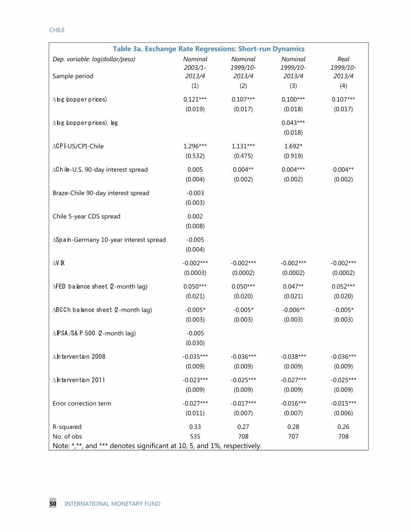
CHILE


Table 3a. Exchange Rate Regressions: Short-run Dynamics Dep. variable: log(dollar/peso) Nominal Nominal Nominal Real

Sample period 2003/1-2013/4

1999/10-2013/4

1999/10-2013/4

1999/10-2013/4

(1) (2) (3) (4)

∆log(copper prices) 0.121*** 0.107*** 0.100*** 0.107***

(0.019) (0.017) (0.018) (0.017)

∆log(copper prices), lag

0.043***

(0.018)

∆CPI-US/CPI-Chile 1.296*** 1.131*** 1.692*

(0.532) (0.475) (0.919)

∆Chile-U.S. 90-day interest spread 0.005 0.004** 0.004*** 0.004**

(0.004) (0.002) (0.002) (0.002)

Braze-Chile 90-day interest spread -0.003

(0.003)

Chile 5-year CDS spread 0.002

(0.008)

∆Spain-Germany 10-year interest spread -0.005

(0.004)

∆VIX -0.002*** -0.002*** -0.002*** -0.002***

(0.0003) (0.0002) (0.0002) (0.0002)

∆FED balance sheet (2-month lag) 0.050*** 0.050*** 0.047** 0.052***

(0.021) (0.020) (0.021) (0.020)

∆BCCh balance sheet (2-month lag) -0.005* -0.005* -0.006** -0.005*

(0.003) (0.003) (0.003) (0.003)

∆IPSA/S& P 500 (2-month lag) -0.005

(0.030)

∆Intervention 2008 -0.035*** -0.036*** -0.038*** -0.036***

(0.009) (0.009) (0.009) (0.009)

∆Intervention 2011 -0.023*** -0.025*** -0.027*** -0.025***

(0.009) (0.009) (0.009) (0.009)

Error correction term -0.027*** -0.017*** -0.016*** -0.015***

(0.011) (0.007) (0.007) (0.006)

R-squared 0.33 0.27 0.28 0.26 No. of obs 535 708 707 708 Note: *,**, and *** denotes significant at 10, 5, and 1%, respectively.

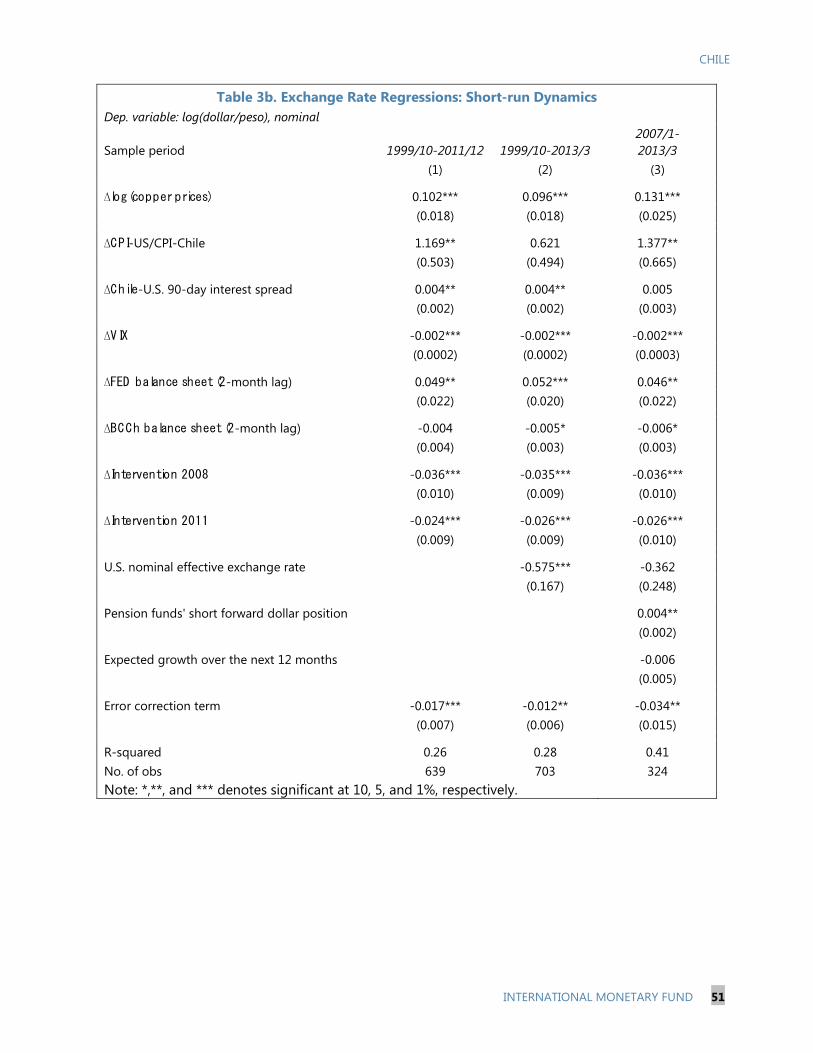
CHILE


Table 3b. Exchange Rate Regressions: Short-run Dynamics Dep. variable: log(dollar/peso), nominal

Sample period 1999/10-2011/12 1999/10-2013/3 2007/1- 2013/3

(1) (2) (3)

∆log(copper prices) 0.102*** 0.096*** 0.131***

(0.018) (0.018) (0.025)

∆CPI-US/CPI-Chile 1.169** 0.621 1.377**

(0.503) (0.494) (0.665)

∆Chile-U.S. 90-day interest spread 0.004** 0.004** 0.005

(0.002) (0.002) (0.003)

∆VIX -0.002*** -0.002*** -0.002***

(0.0002) (0.0002) (0.0003)

∆FED balance sheet (2-month lag) 0.049** 0.052*** 0.046**

(0.022) (0.020) (0.022)

∆BCCh balance sheet (2-month lag) -0.004 -0.005* -0.006*

(0.004) (0.003) (0.003)

∆Intervention 2008 -0.036*** -0.035*** -0.036***

(0.010) (0.009) (0.010)

∆Intervention 2011 -0.024*** -0.026*** -0.026***

(0.009) (0.009) (0.010)

U.S. nominal effective exchange rate

-0.575*** -0.362

(0.167) (0.248)

Pension funds' short forward dollar position

0.004**

(0.002)

Expected growth over the next 12 months

-0.006

(0.005)

Error correction term -0.017*** -0.012** -0.034**

(0.007) (0.006) (0.015)

R-squared 0.26 0.28 0.41 No. of obs 639 703 324 Note: *,**, and *** denotes significant at 10, 5, and 1%, respectively.

CHILE


References

Amano, Robert, and Simon van Norden, 1993, “A Forecasting Equation for the Canada-U.S. Dollar Exchange Rate,” in The Exchange Rate and the Economy, Bank of Canada.

Bloomberg, 2013, “Bernanke-Fueled Rout Avoided by Unwelcoming Chile,” June 5.

Caputo, R., M. Núñez, and R.O. Valdés, 2008, “Análisis del Tipo de Cambio en la Práctica,” Economía Chilena, April, Central Bank of Chile.

Cashin, Paul, Luis F. Cespedes, and Ratna Sahay, 2004, “Commodity Currencies and the Real Exchange Rate,” Journal of Development Economics, Vol. 75, pp.239-268.

Central Bank of Chile, 2007, “Monetary Policy in an Inflation Targeting Framework.”

Chan-Lau, Jorge, 2007, “Foreign Exchange Hedging in Chile,” Derivatives Use, Trading and Regulation, Vol. 12 (3), pp.250-267.

Chen, Yu-Chin, and Kenneth Rogoff, 2003, “Commodity Currencies,” Journal of International Economics, Vol. 60 (1), pp.133-160.

______, 2012, “Are Commodity Currencies an Exception to the Rule?” Journal of Global Economics, Vol. 1 (1).

Chen, Yu-Chin, Kenneth Rogoff, and Barbara Rossi, 2010, “Can Exchange Rates Forecast Commodity Prices?” Quarterly Journal of Economics, Vol. 125, pp.1145-1194.

Cowan, Kevin, David Rappoport, and Jorge Selaive, 2007, “High Frequency Dynamics of The Exchange Rate in Chile,” Central Bank of Chile Working Paper 433.

De Gregorio, José, and Andrea Tokman R, “Flexible exchange rate regime and forex intervention,” Bank for International Settlements Paper 24.

Dickey, D.A. and W.A. Fuller, 1979, “Distribution of Estimators for Autoregressive Time Series with a Unit Root,” Journal of American Statistical Association, Vol. 74, pp.427-431.

Dornbusch, Rudiger, 1976, “Expectations and Exchange Rate Dynamics,” Journal of Political Economy, Vol. 84, pp.1161-1176.

Ghosh, Atish R., and Mahvash S. Qureshi, 2013, “Thinking About Exchange Rates in a World of High Capital Mobility: What We Have Learned in the Past Thirty Years,” International Monetary Fund, memo.

HSBC, 2013, “HSBC’s Emerging Markets Currency Guide 2013.”

CHILE


Helliwell, John, Ramzi Issa, Robert Lafrance, and Qiao Zhang, 2004, “NEMO: An Equation for the Canadian Dollar,” Bank of Canada.

Johansen, Soren, 1991, “Estimation and Hypothesis of Cointegration Vectors in Gaussian Vector Autoregression Models,” Econometrica, Vol. 59, pp.1551-1580.

______, 1995, Likelihood-based Inference in Cointegrated Vector Autoregressive Models Oxford and New York, Oxford University Press.

Larraín, Felipe, 2013, “QE takes a toll on emerging economies,” Financial Times, February 3.

Moazzami, B, and F.J. Anderson, 2003, “Long-term Trend and Short-run Dynamics of the Canadian Dollar: An Error Correction Modeling Approach,” Applied Economics, Vol. 35, pp.1527-1530.

Donal McGettigan, Kenji Moriyama, J. Noah Ndela Ntsama, Francois Painchaud, Haonan Qu, and Chad Steinberg, 2013, “Monetary Policy in Emerging Markets: Taming the Cycle,” International Monetary Fund working paper, forthcoming.

Newey, Whitney K. and Kenneth D. West, 1987, “A Simple Positive Semi-Definite Heteroscedasticity and Autocorrelation Consistent Covariance Matrix.” Econometrica, 55: 703-8.

Stock, J. H., and M. W. Watson, 1993, “A Simple Estimator of Cointegrating Vectors in Higher Order Integrated Systems,” Econometrica, Vol. 61(4): 783-820.

IMF Country Report No. 13/199 CHILE · IMF Country Report No. 13/199 CHILE Selected Issues ......

Documents

Transcript of IMF Country Report No. 13/199 CHILE · IMF Country Report No. 13/199 CHILE Selected Issues ......