Imaris - Bitplane
321
Imaris V 7.2 Reference Manual
Transcript of Imaris - Bitplane
Imaris V 7.2Reference Manual
© Bitplane 2010
1 Preface
This Reference Manual provides a description of all menu entries, display modes, functions and parameters.
Information in this book is subject to change without notice and does not represent a commitment on the partof Bitplane AG. Bitplane AG is not liable for errors contained in this book or for incidental or consequentialdamages in connection with the use of this software.
This document contains proprietary information protected by copyright. No part of this document may bereproduced, translated, or transmitted without the express written permission of Bitplane AG, Zurich,Switzerland.
For further questions or suggestions please visit our web site at: www.bitplane.com or contact [email protected].
Bitplane AGBadenerstrasse 6828048 ZurichSwitzerland
© November 2010, Bitplane AG, Zurich.All rights reserved. Printed in Switzerland.Imaris Reference Manual V 7.2
1.1 Getting Familiar
Today, all optical microscopes commercially available can record several channels simultaneously toproduce multi-channel images. Imaris is an application designed to visualize such microscopic data. Imarisuses a special file format to store images with parameters and can incorporate image files for all majormicroscopes and image acquisition systems. The images can be viewed in several different ways andprocessed to provide the optimum amount of information from 2D or 3D still images, time series, andanimations.
Once a data set has been loaded into Imaris, individual parameters such as channel colors, geometricalsettings or voxel sizes can be adjusted. Imaris has a variety of tools available, such as cropping, thresholdcutting and filters for processing the images to bring out the required details.
It provides 8 different viewing functions for the visualization and production of high quality images forpresentation and storage:
· A Slice viewer.· A Section viewer for simultaneous viewing along three coordinate axes.· A Gallery viewer for slice image overview and selection.· The Easy 3D viewer provides a quick image view.· The Surpass viewer, which offers numerous tools for data preparation, presentation and manipulation of
different types of data display as well as any combination of them and the ability to define, combine andgroup an arbitrary number of objects out of a set of viewing objects.
· Animations can be created from the Slice and 3D modes, or with the key frame animator in Surpass.· InMotion is a 3D viewing and precise interaction mode. Imaris produces a real 3D impression by a smooth
animation of the view. · A viewer for Colocalization computation.
It is easy to navigate within the Imaris modules because the frequently used toolbars, menus, and interactivecontrols remain the same, and can all be operated with the mouse buttons.
Imaris Reference Manual
1.2 Getting Started
The software is delivered on a standard CD or downloaded from www.bitplane.com. The CD includes a foldercontaining the necessary manuals, or the manuals can be downloaded.
Minimum hardware/software requirements are:
· Windows NT 4.0, or a more recent version, Windows 2000, XP, Vista, MacOS X 10.5.0 (Leopard) orhigher
· CD-ROM· Graphics card with 3D accelerator· Network facilities for image import from the microscope· 512 MB RAM (> 1 GB recommended)
Bitplane also recommends:
· A database for storing images (e.g., Image Access)
Installation
To install the software, please proceed as follows:
· Insert your Imaris CD-Rom in the computer.· Follow the instructions on the screen.· The installation is completed automatically.
Licensing
To run the Imaris system, the appropriate licenses for the required modules, such as the Imaris base(including Surpass), ImarisTime, ImarisColoc or Imaris MeasurementPro. Without licenses, the Imaris canonly be run in a restricted mode. In case of any license problems, please refer to the support information onour website www.bitplane.com for detailed instructions.
Starting Imaris
Imaris can be started by one of the following methods:
· Double-click on the Imaris icon (we recommend copying the icon to the desktop).· Drag the icon of an image or a file to the Imaris program icon.· Imaris can be started directly from the Image Access database.
The software opens with the main screen.
Supported File Formats
Imaris (as of version 6.0.0) can read the following file formats, i.e. it can read the image and the parameters.
· Andor: Multi-TIFF series (*.tif, *.tiff)· Andor: MM (*.kinetic)· Applied Precision, Inc: DeltaVision (*.r3d, *.dv)· Biorad: MRC-600, MRC-1024 (series)(*.pic)· BioVision: IPLab Mac (*.ipm)· Bitplane: Imaris 5.5 (*.ims)· Bitplane: Imaris 3.0 (*.ims)· Bitplane: Imaris 2.7 Classic/Old (*.ims)· Bitplane: Imaris Scene File (*.imx)· Carl Zeiss: LSM 510 (*.lsm)· Carl Zeiss: LSM 410, LSM 310 (*.tif, *.tiff)· Carl Zeiss: Axiovision (*.zvi)
© Bitplane 2010
· Compix:Simple PCI (*.cdx)· Image Cytometry Standard: ICS - used by Nikon, Huygens, and others (*.ics, *.ids)· Gatan Digital Micrograph (serie):(*.dm3) · Leica: TCS-NT (*.tif, *.tiff)· Leica: LCS (*.lei, *.raw, *.tif, *.tiff)· Leica: series (*.inf, *.info, *.tif, *.tiff)· Leica: Image File Format (*.lif)· MetaSystem: Meta Viewer (*.imv)· Molecular Devices: Metamorph STK (series) (*.stk)· MRC - primarily electron density volumes as in cryo-EM (*.mrc, *.st, *.rec)· Olympus: FluoViewTIFF (*.tif, *.tiff)· Olympus: 1000 OIF (*.oif)· Olympus: 1000 OIB (*.oib)· Olympus: Cell^R 1.1/standard (*.tif, *.tiff)· Olympus:Virtual Slide Image (*.vsi)· Opellab: liff (series) (*.liff)· Openlab: raw (*.raw)· Open Microscopy Environment XML (*.ome)· Open Microscopy Environment TIF (*.tif, *.tiff)· Perkin Elmer: UltraView (*.tim, *.zpo)· Prairie Technologies: Prairie (*.xml, *.cfg, *.tif, *.tiff)· Scanalytics: IPLab (*.ipl)· TILL Photonics: TILLvisION (*.rbinf)
Plus it can read general TIFF series (or BMP series) of the format aaaNNN.tif (where a is a character and Nis a number).
2 Menu File
Open... Ctrl + ORevert to File Ctrl + RSaveSave as... Ctrl + S
Batch Convert...Scene Viewer...
Batch
Import Scene... Ctrl + LExport Scene... Ctrl + E
Snapshot... Ctrl + T
Exit Ctrl + Q
See also:Addendum - Mouse & Keyboard Mac
2.1 Open
Data sets can be loaded from various file formats.
Image File Series
If the data set consists of a whole series of images, each stored as individual file, select only one file to open
Imaris Reference Manual
and the system will automatically load the rest of the images that belong to the data set.
· In the menu select File – Open.· Select file type from the Files of Type pull-down menu.· Select a file name from the list and click Open or double-click on the requested file entry. The file is loaded.
iQ files in Imaris
To open iQ files in Imaris locate and select the DisckInfo5.kinetic file. Clicking on the ‘Settings’ button opens a new window with a list of images and image information. Check the box Thumbnail Preview to activate an image preview. Select the required image and click on the OK button. Than click again on the Open button. This will instantly create 3D volume rendered image of the selecteddata set.
Button Add to Batch Add to Batch button places the command into Batch coordinator.
See also:Menu File - Batch Convert ...
2.1.1 Reader Configuration
Read only one Time Point
Loads a single time point of a time series.
Resampling Open...
The Resampling Open dialog box can be used as preview before loading a data set and allows you tochange the resolution of the data (subsampling) and to select only a part of the data set (cropping) byspecifying parameters in the Resampling Open dialog box. Both options reduce the size of the data set,decreasing the time needed to read the file and speeding up any operations on the data. This can beparticularly important when reading large data sets over a network.
The revision applies to all views in Imaris and in Surpass.
· Select menu File - Open or click on the button Open in the Main toolbar.· Click on a file to highlight it and click on the button Resampling File Open ... .
Image PreviewThe view on the right side displays as image preview a single time point of the data set. Right-click in theview and move the mouse pointer to the right to increase brightness. Move the pointer upwards to increasecontrast.
Original SizeDisplay of the original file size.
Subsampling Factor
X,Y,Z, Ch, TYou have the option to specify the Subsampling Factor, i.e., the fraction of data points to be retained. Thesubsampling factor can be specified for the x-, y-, z-directions, the channels (Ch), and the time points (T).
Crop Limits (Min/Max)
X, Y, Z, Ch, T, From, ToThe Crop Limits (Min/Max) for the x-, y-, z-directions, the channels (Ch), and the time points (T) can also bespecified.
© Bitplane 2010
Resampled SizeDisplay of the resampled file size.
· Click on OK and the data set is cropped and resampled while loading.
See also:Menu Edit - Image Properties... - GeometryMenu Edit - Crop Time...Menu Edit - Resample Time... Menu Edit - Crop 3D...Menu Edit - Resample 3D...
2.1.2 Settings
In the Settings you specify options for reading certain file formats.
Leica LCS Settings
A LeicaLCS data set consists of a number of image stacks (or experiments). A dialog box can be opened toselect a specific image stack.
· Select File - Open or click Open in the Main toolbar. · Select Files of Type: Leica LCS.· Click on the *.lei file to highlight it and click Settings. A new window appears with a list of images and image information (Name, Description, Recording Date,Data Type, Size, Time Points, Channels, Size (MB), voxel size).
By checking the box Thumbnail Preview possibility of activating an image preview is available. Theindividual images that belong to that stack will display on the left side.
Select the required image stack on the left side of the dialog box.· Click OK to open the image.
Leica LIF Settings
A LeicaLIF data set consists of a number of image stacks (or experiments). A dialog box can be opened toselect a specific image stack.
· Select File - Open or click Open in the Main toolbar. · Select Files of Type: Leica LIF.· Click on the *.lif file to highlight it and click Settings.
A new window appears with a list of images and image information (Name, Description, Recording Date,Data Type, Size, Time Points, Channels, Size (MB), voxel size).
By checking the box Thumbnail Preview the possibility of activating an image preview is available. Theindividual images that belong to that stack will display on the left side.
Select the required image stack on the left side of the dialog box.· Click OK to open the image.
Adjustable Tiff Series Reader Settings
If the data set consists of a series of images, individual images can be sorted according to variousdimensions (i.e., slices, channels, time points, dimension sequence). The selected sequence is shown in theFile Arrangement panel. The reader can handle tiff series with single and multiple running numbers.
· Select the menu File - Open or click Open in the Main toolbar. · Select Files of Type: Tiff (adjustable file series) and not Tiff (series) from the drop-down list.· Open the folder containing the series.
Imaris Reference Manual
· Click Settings, which is grayed out if the file type selector is on automatic or if the current directory does notcontain a series.
· Use Apply Automatic File Filter, Apply, Dimensions, Dimension Sequence, described as follows, to definethe series.
Apply Automatic File
This is activated automatically when the dialog is opened. It has the same logics as the classic TIFF seriesreader of Imaris and will pre-select the first series detected in the directory. Be aware that you may not see allfiles in the directory.
Button ApplyPress this button to use the regular expression to the left and select all files in the current directory thatmatch the criterion, i.e.
· *.tif selects all files with the ending *.tif.· myfile*.tif selects all files that start with ''myfile'' and are followed by any letter or digit and by the extension
*.tif.· myfile??.tif selects all files that start with ''myfile'' and are followed by two letters or digits and by the
extension *.tif.
Please note: Depending on the filter, not all files in the directory may be visible. Selecting the required filemay take some time because every file is opened but only files with identical xy-dimension are chosen.
Dimensions· Define the dimensions of the image starting with Slices (Z), Channels (Ch), and Time Points (T).
Please note: The total number of files in the series, as defined by your selection criteria, displays below theTime Points input box. Selecting the required file may take some time because every file is opened but onlyfiles with identical xy-dimension are chosen.
Dimension Sequence· Defines how the individual images, which are sorted alphabetically, are to be assigned to Slices (Z),
Channels (Ch), and Time Points (T).· Click OK to return to the Open dialog window.· Click Resampling Open to open the Resampling dialog box or click Open to open the image.
2.2 Open in new Window...
This command allows you to open multiple Imaris files.
2.3 Open iQ File ...
Clicking on the Open iQ files opens the Image Selection window with a list of images and imageinformation. Check the box Thumbnail Preview to activate an image preview.Select the required image and click on the OK button. This will instantly create a 3D volume rendered image of the selected data set.
Search File NameSearch for all files that meet a desired criteria
Resample Open ButtonResampling Open...
The Resampling Open dialog box can be used as preview before loading a data set and allows you tochange the resolution of the data (subsampling) and to select only a part of the data set (cropping) byspecifying parameters in the Resampling Open dialog box. Both options reduce the size of the data set,
© Bitplane 2010
decreasing the time needed to read the file and speeding up any operations on the data.
Image PreviewThe view on the right side displays as image preview a single time point of the data set. Right-click in theview and move the mouse pointer to the right to increase brightness. Move the pointer upwards to increasecontrast.
Original SizeDisplay of the original file size.
Subsampling Factor
X,Y,Z, Ch, TYou have the option to specify the Subsampling Factor, i.e., the fraction of data points to be retained. Thesubsampling factor can be specified for the x-, y-, z-directions, the channels (Ch), and the time points (T).
Crop Limits (Min/Max)
X, Y, Z, Ch, T, From, ToThe Crop Limits (Min/Max) for the x-, y-, z-directions, the channels (Ch), and the time points (T) can also bespecified.
Resampled SizeDisplay of the resampled file size.
· Click on OK and the data set is cropped and resampled while loading.
2.4 Revert to File
Re-opens the actual data set.
2.5 Save
To save an existing dataset click Save in the File menu or Save icon on the Main toolbar.
2.6 Save as ...
Saving in Imaris format is recommended whenever the data set is cropped or the parameters changed.Saving a data set in Imaris file format provides the advantage of a faster loading process and the possibilityof using thumbnails. In addition, parameters are saved with the images.The standard way to save your data and Imaris scene is simply to choose Save as from the File menu andgive an appropriate name. The file extension, suggested as the default, is *.ims. The single created Imarisfile contains both the image and the scene data. You can save the file when you are done or if you want you can stop in the middle and resume work later.Simply, choose Save as from the File menu and give the file a name you will remember. If you then close thefile and reopen it at a later time, you can resume work from where you left off.
· In the menu bar select File - Save as.... The Save as window displays.· Select the directory and enter the name for the file to be saved or confirm the suggestion.· Select the requested file format and click OK.
The data set is saved.
Available File Formats in Imaris
Bitplane: Imaris 5.5 (*.ims)Bitplane: Imaris 3.0 (*.ims)Bitplane: Imaris 2.7 (Classic)(*.ims)
Imaris Reference Manual
Tiff (series)(*.tif *.tiff)RGBA-Tiff (series)(*.tif *.tiff)ICS file (*.ics *.ids)Olympus: cell^R 1.1/standard (*.tif *.tiff)Open Microscopy Environment XML (*.ome)Open Microscopy Environment Tiff (*.tif *.tiff)BMP (series)(*.bmp)Move file (slice animation) (*.avi, *.mov, *.tif, *.tiff)
Export and Import Scene File
The actual Imaris configuration (including Surpass Tree and all existing Items) in the Surpass view is calledSurpass Scene and can be stored in a Scene file with the extension *.imx. The Surpass Scene can be loadedagain to the same data set or to another data set. For details please refer to chapter Surpass View -Overview - Scene File Concept.
Button Add to Batch Add to Batch button places the command into Batch coordinator.
See also:Menu File - Batch Convert...
2.6.1 Advanced Save Options
Button Format Settings...A click on the button Format Settings... opens the Imaris Save Options window.
Window: Save OptionsBitplane: Imaris 5.5 (*.ims)
Enable Compression Check the box to use compression.
Export Scene Check the box to save the Imaris scene.
Bitplane: Imaris 3.0 (*.ims)
Time SeriesSave as Single FileThe time series are saved in a single file.
Save as Multiple FilesFor each time point a new file is generated.
CompressionLZW CompressionCheck the box to use an LZW compression.
Add to ImageAccess Database
Check the box to add the file to the ImageAccess database.
2.7 Batch Convert ...
With the Imaris File Converter you can convert various image file formats to the Imaris file format *.ims.Select the menu entry Batch Convert... and the Imaris File Converter window displays. From the WindowsStart menu select "ImarisFileConverter".
© Bitplane 2010
Input
Drag & Drop Files, or click the Button below to add Files.
Button Add Files ...The window Select Files for Conversion displays. Choose the respective file and click on the Add Files...button.
Thumbnail
Here you can select the appearance of the thumbnail in Imaris.
Middle SliceThumbnail is the middle slice.
MIPThumbnail in the display mode Maximum Intensity Projection. A Maximum Intensity Projection is a computervisualization method for 3D data that projects in the visualization plane the voxels with maximum intensitythat fall in the way of parallel rays traced from the viewpoint to the plane of projection.
Blend Thumbnail in blend projection. Blends all values along the viewing direction and includes their transparency.
Output
Same Folder as Input FileYou find the converted image(s) in the same folder as the input files.
Special FolderHere you can select another folder for the converted image(s). Either type in the respective path or use thebutton Browse.
Button BrowseClick on this button to browse for the special folder.
Button Set for AllClick on this button and all converted image(s) are saved in the designated folder.
FormatHere you can select the format of the output files.The standard formats are:Bitplane: Imaris 5.5 (*.ims)Bitplane: Imaris 3.0 (*.ims)Bitplane: Imaris 2.7 (Classic)(*.ims)
To add additional formats please refer to chapter Menu File - Batch Convert ... - Preferences.
Input
Here you find the selected input file path(s).
Click on the input path to open the window Series Reading Sequences to adjust additional parameters for theconversion. Please refer to chapter Menu File - Open - Settings for details.
Output
Here you find the selected output file path(s).
Click on the output path to open the window Imaris Save Options to adjust additional parameters for theconversion. Please refer to chapter Menu File - Save as ... - Advanced Save Options for details.
Imaris Reference Manual
Clear Row
To clear a row click on the red cross at the end of the row.
Button ClearClick on this button to clear all rows in the table.
Button StartClick on this button to start the conversion.
See also:Menu File - Open - Reader ConfigurationMenu File - Open - SettingsMenu File - Save as ... - Advanced Save OptionsMenu File - Batch Convert ... - Preferences
2.7.1 Preferences
Button PreferencesClick on this button to open the Preferences window.
Window: Preferences
Data Cache
Imaris utilizes advanced data caching mechanism that allows you to process images that are significantlylarger than the physical memory (RAM) installed in the computer system. This mechanism writes image datablocks to the disk and reads them back into the physical memory when they are needed. Cache File Paths displays the cache file location.
Please note: Setting the Cache File location to an unused disc, improves the performance when working onlarger images. This benefits a lot from a fast SSD with a minimum size of 10 times the biggest dataset, whichwill be used.
Memory Limit (MB)The value of Data cache limit controls the amount of data blocks Imaris will keep in memory at any time.
File Paths:Display of the cache file paths.
Button AddYou can use the buttons to add file paths in the list.
Button RemoveYou can use the buttons to remove file paths in the list.
Output Formats
If you want to extend the list of output formats you have to check the following parameter and enter a validlicense in the next step. Find your licence number in Imaris as follows: Click on the menu Help, select themenu entry Licenses and copy the license number (in the License Path at the bottom of the window, next tolast enter field).
Include Image FilenamesSelect this option and the output file names are assigned by using a default-naming rule.
Suffix AlphabeticThe output file inherits the input file name followed by the successive alphabetic letter.
Suffix Numeric
© Bitplane 2010
The output file inherits the input file name followed by the number of the output files being created(consecutive integer numbers).
All Imaris Output File FormatsCheck this box to extend the output file formats.
License LocationType in your license number or use the button Browse.
Button BrowseClick on this button and select the license path.
Button OKClick on this button and all available Imaris output formats are available.
Standard formats:Bitplane: Imaris 5.5 (*.ims)Bitplane: Imaris 3.0 (*.ims)Bitplane: Imaris 2.7 (Classic)(*.ims)
Additional formats:Tiff (series)(*.tif *.tiff)RGBA-Tiff (series)(*.tif *.tiff)ICS file (*.ics *.ids)Olympus: cell^R 1.1/standard (*.tif *.tiff)Open Microscopy Environment XML (*.ome)Open Microscopy Environment Tiff (*.tif *.tiff)BMP (series)(*.bmp)
See also:Menu File - Save as ...
2.8 Scene Viewer...
To start Imaris Scene Viewer from Imaris click on the Scene Viewer option.
2.9 Batch
To start Imaris Batch Coordinator from Imaris click on the Batch option.
2.10 Inport Scene ...
A Scene comprises the Surpass Tree including all existing Items. The Scene can be loaded again to thesame data set or to another data set. The Scene can be loaded as an Imaris Scene File with the extension *.imx or as an Imod Binary File with theextension *.imod and *.mod. The Imod Scene, with *.imod and *.mod extensions, contains Surpass objects: Spots, Surfaces andContour Surfaces.
Load Imaris Scene...
Select the directory and requested file to be loaded, and click OK. The Scene File is loaded.
To adjust which objects of the Imod scene are loaded, select the Edit menu- Preference-AdvancedParameters – FileLoading.To control which part of the imod scene is loaded, alter the setting of the parameters (true / false):ImodSceneLoadContourImodSceneLoadWildContoursImodSceneLoadSurfaces
Imaris Reference Manual
See also:Menu File - Export Scene...Surpass View - Overview - Surpass TreeSurpass View - Overview - Scene File Concept
2.11 Export Scene
A Scene comprises the Surpass Tree including all existing Items. This Scene can be saved as an ImarisScene File with the extension *.imx. The Scene can be loaded again to the same data set or to another dataset.
Save Imaris Scene
Select the directory and enter the Scene File name and click OK. The Surpass Tree Items are saved asImaris Scene File.
See also:Menu File - Import Scene... ...Surpass View - Overview - Surpass TreeSurpass View - Overview - Scene File Concept
2.12 Snapshot
Snapshot captures a 2D image of the 2D, 3D or 4D image data as it currently appears in the viewing area. Itcreates a new file containing your image as well any scale information, measurements data, and ROI that aredisplayed. The snapshots can be (1) stored in TIFF-Format, (2) saved as database records in ImageAccessin order to manage them more efficiently or else (3) copied to the clipboard.
The Image Size settings specify the size of a Snapshot. The snapshot size (in pixels) is equal to the settingsin the width/height numerical fields. The default setting for snapshot size is the Snapshot size from window size option. To modify and customizesnapshot dimensions you can either select the predefined sets from the drop-down list or manually adjust the Width and Height values.Adjusting the width or height settings for the snapshot changes the number of pixels in the snapshot, byresampling and/or cropping/expanding the image in the viewing area to match the specified pixel dimensions.The placement of the snapshot borders (cropping or expansion) depends on the aspect ratio of the viewingarea compared to the snapshot aspect ratio, and the setting called Crop to fill whole snapshot area (seebelow). Changing the snapshot dimensions scales the input image, so that none of its dimensions are greater thanthe corresponding snapshot (output image) dimension. The scaled image is centered within the newsnapshot size. In other words, the zoom of the input image is automatically scaled to better fit the availablepixels in the snapshot. Depending on the settings used, some of the background color might also beconsidered to be part of the input image.When the aspect ratio of the viewing area does not match the aspect ratio of the snapshot, the snapshot issurrounded with bars in the color of the Imaris screen background. There are two options allowing the user toadjust the content of the snapshot and to eliminate the Imaris screen background. The image can be eitherscaled to fit the selected snapshot dimensions (by adjusting the zoom in the viewing area) or else the Crop tofill whole snapshot area option can be used.
Snapshot preview
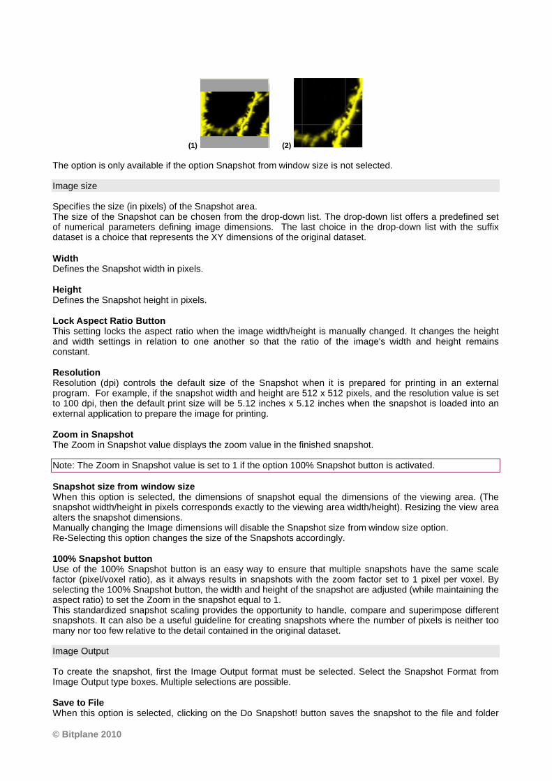
Snapshot preview offers a view of the snapshot content, as it will look when finalized. Crop to fill whole snapshot area This option crops the image to fit the snapshot specified Width and Height values. The option sets an imageso that one dimension fits the snapshots viewing area, while the overflow of the other dimension is cut off,respecting image aspect ratio. The images below illustrate Pyramidal cell image Snapshots taken with the various settings. (1) Disparitybetween image size and snapshot intended dimensions, (2) Crop to fill whole snapshot area.
© Bitplane 2010
(1) (2)
The option is only available if the option Snapshot from window size is not selected.
Image size
Specifies the size (in pixels) of the Snapshot area. The size of the Snapshot can be chosen from the drop-down list. The drop-down list offers a predefined setof numerical parameters defining image dimensions. The last choice in the drop-down list with the suffixdataset is a choice that represents the XY dimensions of the original dataset.
WidthDefines the Snapshot width in pixels.
HeightDefines the Snapshot height in pixels.
Lock Aspect Ratio ButtonThis setting locks the aspect ratio when the image width/height is manually changed. It changes the heightand width settings in relation to one another so that the ratio of the image's width and height remainsconstant.
Resolution Resolution (dpi) controls the default size of the Snapshot when it is prepared for printing in an externalprogram. For example, if the snapshot width and height are 512 x 512 pixels, and the resolution value is setto 100 dpi, then the default print size will be 5.12 inches x 5.12 inches when the snapshot is loaded into anexternal application to prepare the image for printing.
Zoom in SnapshotThe Zoom in Snapshot value displays the zoom value in the finished snapshot.
Note: The Zoom in Snapshot value is set to 1 if the option 100% Snapshot button is activated.
Snapshot size from window size When this option is selected, the dimensions of snapshot equal the dimensions of the viewing area. (Thesnapshot width/height in pixels corresponds exactly to the viewing area width/height). Resizing the view areaalters the snapshot dimensions. Manually changing the Image dimensions will disable the Snapshot size from window size option.Re-Selecting this option changes the size of the Snapshots accordingly.
100% Snapshot buttonUse of the 100% Snapshot button is an easy way to ensure that multiple snapshots have the same scalefactor (pixel/voxel ratio), as it always results in snapshots with the zoom factor set to 1 pixel per voxel. Byselecting the 100% Snapshot button, the width and height of the snapshot are adjusted (while maintaining theaspect ratio) to set the Zoom in the snapshot equal to 1.This standardized snapshot scaling provides the opportunity to handle, compare and superimpose differentsnapshots. It can also be a useful guideline for creating snapshots where the number of pixels is neither toomany nor too few relative to the detail contained in the original dataset.
Image Output
To create the snapshot, first the Image Output format must be selected. Select the Snapshot Format fromImage Output type boxes. Multiple selections are possible.
Save to FileWhen this option is selected, clicking on the Do Snapshot! button saves the snapshot to the file and folder
Imaris Reference Manual
specified in the snapshot name field. You can either accept the automatic naming suggestion or enter a newname for the image the name field.
Copy to ClipboardWhen this option is selected, clicking on the Do Snapshot! button copies the snapshot to the clipboard.Open another application and use the paste function.
Add to ImageAccess DatabaseMake sure that the database ImageAccess is started. In ImageAccess, select the requested directory andenter a name for the image. Then in Imaris click on the Do Snapshot! button and the image is saved on thedisk and an entry is added to the database.
Snapshot nameThis field specifies under which folder and filename the snapshot will be saved. Initially, the automaticnaming suggestion is displayed. Snapshots are automatically placed in the same directory with the samename as the original dataset and a sequential number is inserted at the end of the name. This 3-digit trailingnumber will automatically increment by one each time you click Do Snapshot!, to save the user the trouble ofmanually typing a new filename each time.
Do Snapshot! buttonClick on the Do Snapshot! button to create the image snapshot.
See also:Menu Edit - Copy Snapshot ImageMenu Edit - Preferences - Display - Off Screen RenderingToolbars - Main Toolbar - Snapshot
2.13 Exit
Terminates Imaris and returns to the desktop.
3 Menu Edit
Undo Ctrl + ZCopy Snapshot Image Ctrl + C
Image Properties... Ctrl + IShow Display Adjustment Ctrl + D
InPress Ctrl + Shift + P
Add Time Points...Delete Time Points...Add Channels... Ctrl + Shift + ADelete Channels... Ctrl + Shift + BAdd Slices...Delete Slices...
Crop Time...Resample Time...Crop 3D... Ctrl + WResample 3D...Change Data Type...
Preferences... Ctrl + PFile Type Associations...
© Bitplane 2010
See also:Addendum - Mouse & Keyboard Mac
3.1 Undo
The Undo command reverses the last action, when necessary. It supports multiple undo actions, starting withthe most recent one and working backwards in sequence.
All actions in the Draw , Edit and Edit Tracks tabs as well as the image processing functions can beundone by selecting the Undo command or by pressing Ctrl+Z.The number of any previously applied command that can be Undone/Redone is defined in the Editmenu-Preferences-Calculations-Maximum Number of Commands in History filed. By default, the numberof steps is 4.
3.2 Redo
The Redo command repeats the last action, if appropriate. The command supports multiple redo actions,starting with the most recent one and working backwards in sequence.
All action in the Edit, Edit tracks, and Draw tabs as well as image processing functions can be redone byselecting the Redo command or by pressing Ctrl+Y.
The number of any previously applied command that can be Undo/Redo is defined in the Editmenu-Preferences-Calculations-Maximum Number of Commands in History filed.
3.3 Copy Snapshot Image
When an image is ready to be stored, make sure that it is fully visible on the screen and not obstructed byany other windows or displays. To save the image, Imaris reads from the internal buffer, so other objects onthe screen would appear superimposed on the image.
· Select Edit - Copy Snapshot Image and the image is copied to the clipboard.
Open another application and select the paste function. The image is pasted into the new application.
See also:Menu File - Snapshot
3.4 Image Properties...
GeometryData SetChannels (Channel 1...n)ThumbnailParameters
When opening a data set, the following parameters should be checked or modified:
· Name and Description (in Data Set).· Voxel Sizes (in Geometry).· Channel Colors (in Channel 1...n).
Imaris Reference Manual
3.4.1 Geometry
The geometrical settings of the actual data set are displayed.
Type
Data TypeDisplay of the image type.
Size
Size X, Y, Z, TDisplay of the image size.
Coordinates
Voxel Size, X, Y, ZThe voxel sizes directly influence the views because they control the height of the image relative to its width.Check the parameters and adjust the Voxel Size and/or other settings if necessary.
Min, X, Y, ZThe minimum value of the coordinate axes.
Max, X, Y, ZThe maximum value of the coordinate axes.
Unit, nm, um, mm, m, unknownHere you can select the unit.
Button Add to Batch Add to Batch button places the command into Batch coordinator.
Time Point
First BoxSelect the time point.
DateEnter the collection data.
Time Enter the collection time.
Button All Equidistant...If the data set is a time series, enter the date/time for each time point or click All Equidistant to open the SetEquidistant Time Points dialog box.
· Enter the Start Date and Start Time and the Time Interval.· Click OK when finished. Imaris will calculate the time for each time point in the series.
The data set must be saved to retain the changes. Click OK when finished or select another heading forfurther adjustments.
Button OKTo apply the changes click on OK.
Button Add to Batch Add to Batch button places the command into Batch coordinator.
Button CancelIf you do not want to save the changes click on Cancel.
© Bitplane 2010
3.4.2 Data Set
Name
Data field to type in a data set name.
Description
Data field to type in a data set description.
Numerical Aperture (N.A.)
Reads out the numerical aperture (as defined in the menu Edit - Image Properties... - Parameters).
Log
Display of processing steps.
Button OKTo apply the changes click on OK.
Button CancelIf you do not want to save the changes click on Cancel.
3.4.3 Channels
There is no parameter on this card.
3.4.4 Channel 1...n
In the Index of the Image Properties box click the Channel entry (Channel 1, Channel 2 etc.) to select therequired channel.
Name
Data field to type in the channel name.
Description
Data field to type in a channel description.
Emission Wavelength
Reads out the emission wavelength.
Excitation Wavelength
Reads out the excitation wavelength.
Pinhole Radius
Reads out the pinhole radius.
Button OKTo apply the changes click on OK.
Imaris Reference Manual
Button CancelIf you do not want to save the changes click on Cancel.
3.4.4.1 Tab Base Color
Red, Green, BlueReads out the assigned color. To change the color either adjust the values or move the square in the colorcircle.
To apply the changes click on OK.
3.4.4.2 Tab Mapped Color
Selected Color
Button Edit...Click on a square in the grid and click on the button Edit... . Select a color and click on OK. The selectedcolor is displayed in the square.
Button CopyClick on a square in the grid and then on the button Copy to copy the color.
Button PasteClick on a square in the grid and then on the button Paste to paste the color.
Interpolation
ColorspaceRGBThe RGB color model is an additive model in which red, green and blue are combined in various ways toreproduce other colors.
HSVThe HSV (Hue, Saturation, Value) model, defines a color space in terms of three constituent components.
· Hue, the color type.· Saturation, the vibrancy of the color.· Value, the brightness of the color.
Button InterpolateSelect two squares in the grid and click on the button Interpolate. The colors between the two selectedsquares are interpolated.
Color Table File
Button Import ...Imaris comes with a set of pre-defined color tables. Click on Import... to open the Import Color Table Filewindow. Select a color table file and click on OK.
Button Export...Click on the button Export... to open the Export Color Table File window. Select a destination and click onSave.
To apply the changes click on OK.
© Bitplane 2010
3.4.4.3 Tab Coloc Statistics
The tab Coloc Statistics is available when a data set contains a Coloc channel and the Coloc channel isselected in the channel selection of the Image Properties.
All statistics about the resulting colocalized volume are displayed. Definitions of the displayed values andfurther information are given in chapter Coloc - Volume Statistics.
Button Export...Click on the button Export... to open the Export Color Table File window. Select a destination and click onSave.
See also:Coloc - Volume Statistics
3.4.5 Thumbnail
Type
NoneSelect None if no thumbnail should be displayed.
Middle SliceThumbnail is the middle slice.
MIPThumbnail in the display mode Maximum Intensity Projection. A Maximum Intensity Projection is a computervisualization method for 3D data that projects in the visualization plane the voxels with maximum intensitythat fall in the way of parallel rays traced from the viewpoint to the plane of projection.
Blend Thumbnail in blend projection. Blends all values along the viewing direction and includes their transparency.
Preview
Displays a preview of the thumbnail image.
Button OKTo apply the changes click on OK.
Button CancelIf you do not want to save the changes click on Cancel.
3.4.6 Parameters
A set of informational parameters is appended to the image file.
Button Add Group...Opens a dialog to add a new group.
Button Delete Group...Deletes a group.
Button Add Parameter...Opens a dialog to add a new parameter to the group.
Button Delete Parameter...Deletes a parameter.
Imaris Reference Manual
Button OKTo apply the changes click on OK.
Button CancelIf you do not want to save the changes click on Cancel.
3.5 Show Display Adjustments
The Display Adjustment function lets you choose the channel visibility as well as improve the image displayby concentrating on a limited color contrast range of voxels. Usually the color contrast values of the voxelsstretch over a wide range (e.g. 0 - 255).
The Display Adjustment function lets you set an upper limit for maximum color and a lower limit for minimumcolor (i.e., black). The range between these two limits is then extrapolated in a linear mode to the full data setrange and the new voxel values are calculated.
Display Adjustment Dialog (one for each channel)
Switch the individual channels on or off. · Check or un-check the required channel check-box to switch the channel visibility.
Change the channel parameters such as name, color and description. · Click on the channel name to open the Image Properties. For a detailed description please refer to chapter
Menu Edit - Image Properties - Channels 1...n.
Button AdvancedClick on the button to open the Advanced settings (see below).
Select all ChannelsCheck Select all Channels to apply the settings to all channels.
Advanced Settings
MinMax· Enter direct values in the Min (lower limit for minimum color) and Max (upper limit for maximum color)
fields. · Alternatively drag in the display adjustment dialog the upper or lower handle of the adjustment line to adjust
the Min and Max limits. The effect of the change can be seen on the channels (channels appear brighter or darker).
GammaThe default value of the gamma correction is 1 (the range between lower and upper limit is extrapolated in alinear mode to the full data set range). Enter a value below 1 and the linear mode is transferred to a nonlinearmode, the lower intensities appear brighter. The effect of the change is directly visible in the viewing area. · Enter the value in the respective field.· Alternatively click onto the middle triangle in the display adjustment dialog and drag it to the left to increase
brightness/to the right to decrease brightness.
OpacityThe blend opacity adjustment allows you to change the opacity in real-time in blend projections in Section,Full 3D, and Surpass Volume views. · Drag the blend opacity slider bar to adjust the blend opacity.
Moving the slider to the left reduces the blend opacity, moving it to the right increase blend opacity.· Alternatively right-click in the display adjustment dialog and drag the mouse to adjust the values.The effect of the change can be seen on the channels (channels appear more or less transparent).
List of Shortcuts in the Display Adjustment Dialog
© Bitplane 2010
Please refer to chapter Menu Edit - Show Display Adjustments - Mouse & Keyboard PC.Please refer to chapter Menu Edit - Show Display Adjustments - Mouse & Keyboard Mac.
Button ResetClick the Reset button to set the image back to the original values.
Button AutoWhen clicking the button Auto the system detects the real high and low values (e.g. 10 - 150) and sets theMax. and Min. limits automatically to these values. If you check the parameter Select all Channels (see above) all channels are calculated consecutively.
Button Auto BlendThis button is useful if you display your data in the Blend mode (item Volume - tab Settings - Mode Blend). Click on this button and Imaris automatically calculates the optimized Min. and Max. limits. A good portion ofthe selected image channel becomes transparent.If you check the parameter Select all Channels (see above), all channels are calculated consecutively.
Button Add to Batch Add to Batch button places the command into Batch coordinator.
Histogram
A histogram is a statistical data analysis, representing linear voxel within an image of the selected channel.
Change Channel Color
Click on the channel name to switch directly to the channel properties (Menu Edit - Image Properties -Channels 1...n).
See also:Menu Edit - Image Properties... - Channel 1...nMenu Edit - Show Display Adjustments - Mouse & Keyboard PCMenu Edit - Show Display Adjustments - Mouse & Keyboard Mac
3.5.1 Mouse & Keyboard PC
Mouse & Keyboard Functions in the Display Adjustments Window
Ctrl + D Shows the Display Adjustment windowLeft-click Select channelLeft-click onmiddle triangle anddrag
Adjust Gamma Correction
Ctrl + left-click Add channel to selection, or remove channel from selectionLeft-click & drag Move left: make image channel brighter
Move right: make image channel darkerMove up: increase image channel contrastMove down: decrease image channel contrast
Right-click & drag Move left: make image channel transparentMove right: make image channel opaque
Ctrl + right-click Automatic range for Min and Max
See also:Addendum - Mouse & Keyboard PC
3.5.2 Mouse & Keyboard Mac
Mouse & Keyboard Functions in the Display Adjustments Window
Imaris Reference Manual
Command + D Shows the Display Adjustment windowClick Select channelLeft-click on middletriangle and drag
Adjust Gamma Correction
Command + click Add channel to selection, or remove channel from selectionClick & drag Move left: make image channel brighter
Move right: make image channel darkerMove up: increase image channel contrastMove down: decrease image channel contrast
Ctrl + click & drag Move left: make image channel transparentMove right: make image channel opaque
Command + Ctrl + click Automatic range for Min and Max
See also:Addendum - Mouse & Keyboard Mac
3.6 InPress
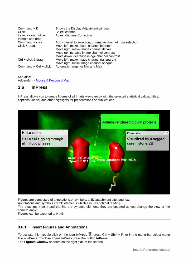
InPress allows you to create figures of all Imaris views ready with the selected statistical values, titles,captions, labels, and other highlights for presentations or publications.
Figures are composed of annotations or symbols, a 3D attachment site, and text.Annotations and symbols are 2D elements which assures optimal reading.The attachment point and the line are dynamic elements they are updated as you change the view or thecamera angle.Figures can be exported to Html.
3.6.1 Insert Figures and Annotations
To activate this module click on the Icon InPress , press Ctrl + Shift + P, or in the menu bar select menuFile – InPress. To close Imaris InPress press the button InPress.The Figures window appears on the right side of the screen.
© Bitplane 2010
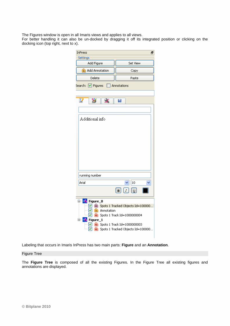
The Figures window is open in all Imaris views and applies to all views.For better handling it can also be un-docked by dragging it off its integrated position or clicking on thedocking icon (top right, next to x).
Labeling that occurs in Imaris InPress has two main parts: Figure and an Annotation.
Figure Tree
The Figure Tree is composed of all the existing Figures. In the Figure Tree all existing figures andannotations are displayed.
Imaris Reference Manual
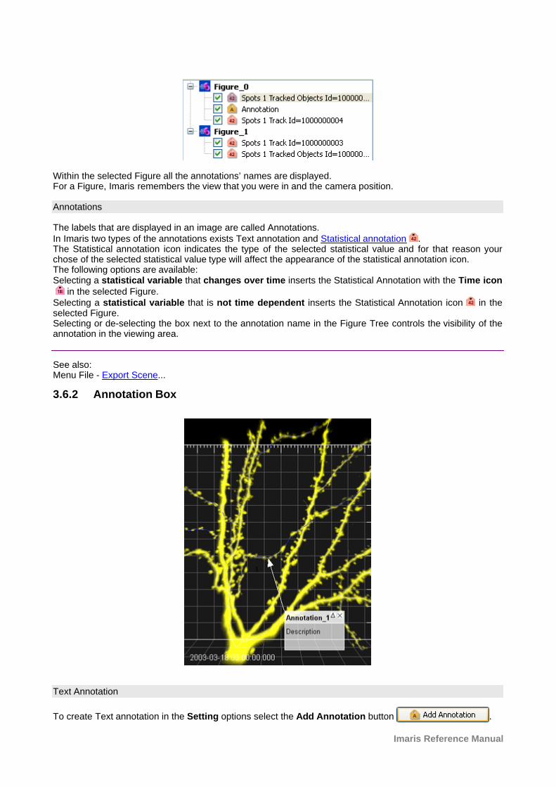
Within the selected Figure all the annotations’ names are displayed.For a Figure, Imaris remembers the view that you were in and the camera position.
Annotations
The labels that are displayed in an image are called Annotations.In Imaris two types of the annotations exists Text annotation and Statistical annotation .The Statistical annotation icon indicates the type of the selected statistical value and for that reason yourchose of the selected statistical value type will affect the appearance of the statistical annotation icon. The following options are available:Selecting a statistical variable that changes over time inserts the Statistical Annotation with the Time icon in the selected Figure. Selecting a statistical variable that is not time dependent inserts the Statistical Annotation icon in theselected Figure. Selecting or de-selecting the box next to the annotation name in the Figure Tree controls the visibility of theannotation in the viewing area.
See also:Menu File - Export Scene...
3.6.2 Annotation Box
Text Annotation
To create Text annotation in the Setting options select the Add Annotation button .
© Bitplane 2010
To create Text annotation box click in the image to set the 3D anchor point. Move the mouse to elongate the line. With the second click you fix the top left corner of the text box. Move the mouse to adjust the text box size. With the third click you fix the text box size.
Statistical Annotations
By default, statistical annotations are presented in the viewing area without an annotation box. To createthe annotation box for the statistical annotations select the annotation in the Figure Tree, and then activate
the Text box option under the Style tab .
The position of the statistical annotations can be adjusted by moving the annotation box and the anchor area.
The statistical annotation is assigned to the selected objects in the image and the anchor point cannot beplaced on another object.
Once created the annotation box and anchor point can be moved to the preferred location.
Move Annotation Point, Box, Number
To move the 3D anchor point set the mouse over the anchor point (until it changes to a cross) then click &drag to a new location.To move the annotation box set the mouse on the upper region of the box (until it changes to a cross) thenclick & drag to a new location.To move the annotation number set the mouse over it (until it changes to a cross) then click & drag to anew location.
Resize the Annotation Box
To resize the annotation box set the mouse to an edge of the box (until the mouse changes to a resize icon)and then click & drag the edge.
Annotation Visibility
The description area of the annotation can be closed (hidden) or expanded (shown) by clicking the triangleon the top right of any annotation box.The annotation can be hidden by clicking the “X” on the top right corner of the box. Selecting or de-selecting the box next to the annotation name in the Figure tree controls the visibility of theannotation in the viewing area.
Save Figures and Annotations in Scene File
The figure legends are saved in the scene file of a data set.
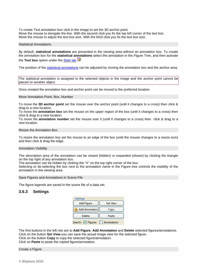
3.6.3 Settings
The first buttons in the left row are to Add Figure, Add Annotation and Delete selected figures/annotations. Click on the button Set View you can save the actual image view for the selected figure. Click on the button Copy to copy the selected figure/annotation. Click on Paste to paste the copied figure/annotation.
Create a Figure
Imaris Reference Manual
Click on Add Figure. In the first row of the tab Text the standard text header Figure_0 is displayed. To namea figure type the name in the text box. In the second row you can add a figure description. A figure label appears in the Imaris InPress Tree. To jump to the view and camera position associated with a figure double-click the figure name in the FigureTree. To change the view associated with a particular figure, highlight the name of the figure in the list, moveto the Imaris view of interest, and press the button Set View from the Settings of Imaris InPress
How to Create Text Annotations
Annotations can be added to any figure you want to create. First you have to select the Figure name in the Figure Tree.The Figure name is highlighted. Click on Add Annotation. In the first row of the tab Text the standard text header Annotation_0 is displayed. To edit the annotation title select the Text tab . In the Annotation title description window write newdescription. In the second row you can add an annotation text.
Search for Figures and Annotations
You can search for the initials in the title field (first row on the tab Text) of a Figure or Annotation.
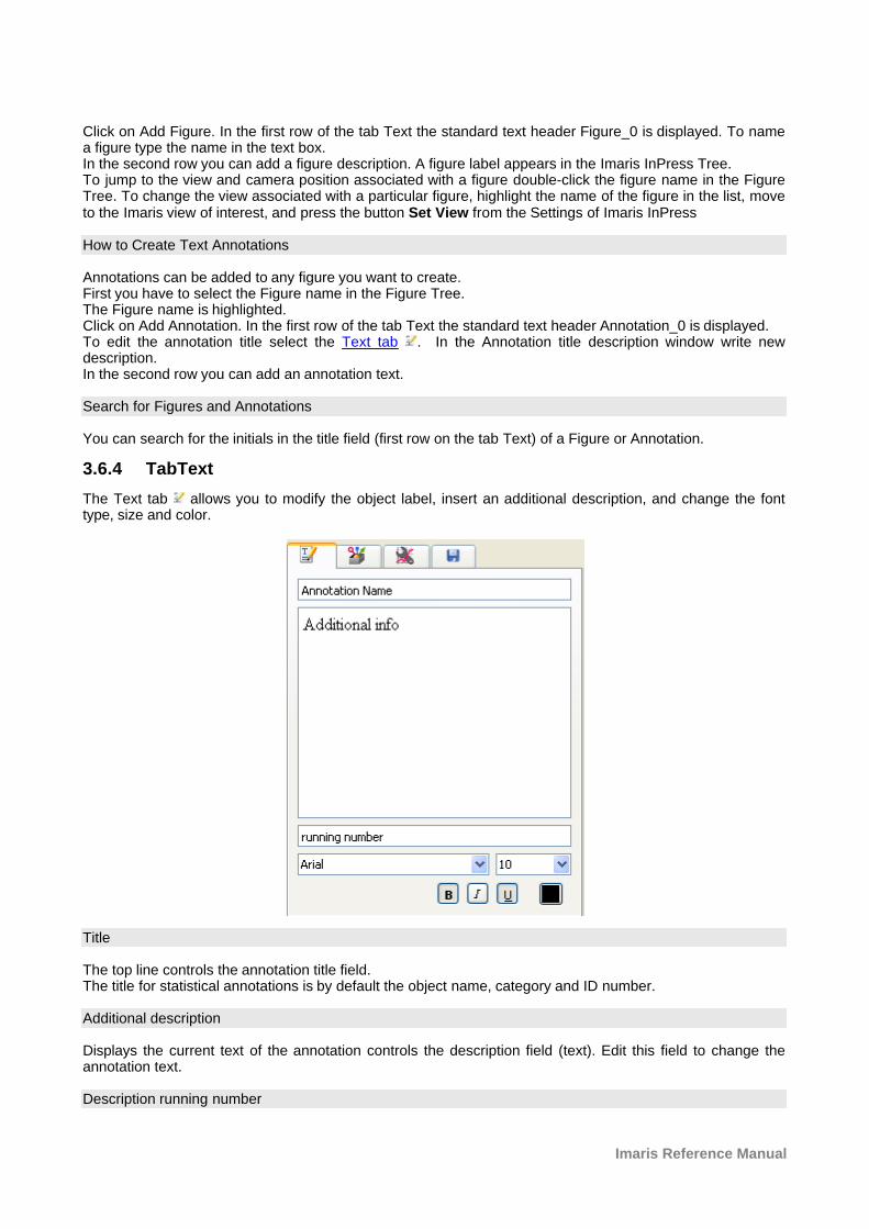
3.6.4 TabText
The Text tab allows you to modify the object label, insert an additional description, and change the fonttype, size and color.
Title
The top line controls the annotation title field.The title for statistical annotations is by default the object name, category and ID number.
Additional description
Displays the current text of the annotation controls the description field (text). Edit this field to change theannotation text.
Description running number
© Bitplane 2010
The third box by default contains the annotation running number (legend). To remove the number from theimage, delete it from the text field
FontSelect this option to adjust the appearance of the text.The parameter specifies the name of the font to use for the text. This font must be supported on your system,in order to be displayed and printed properly. The default font is Arial. This value specifies the font size. Thedefault size is 10.
All changes made in the Text Tab are applied for all time points.
To display the default settings click on the menu Edit - Preferences... and select InPress.
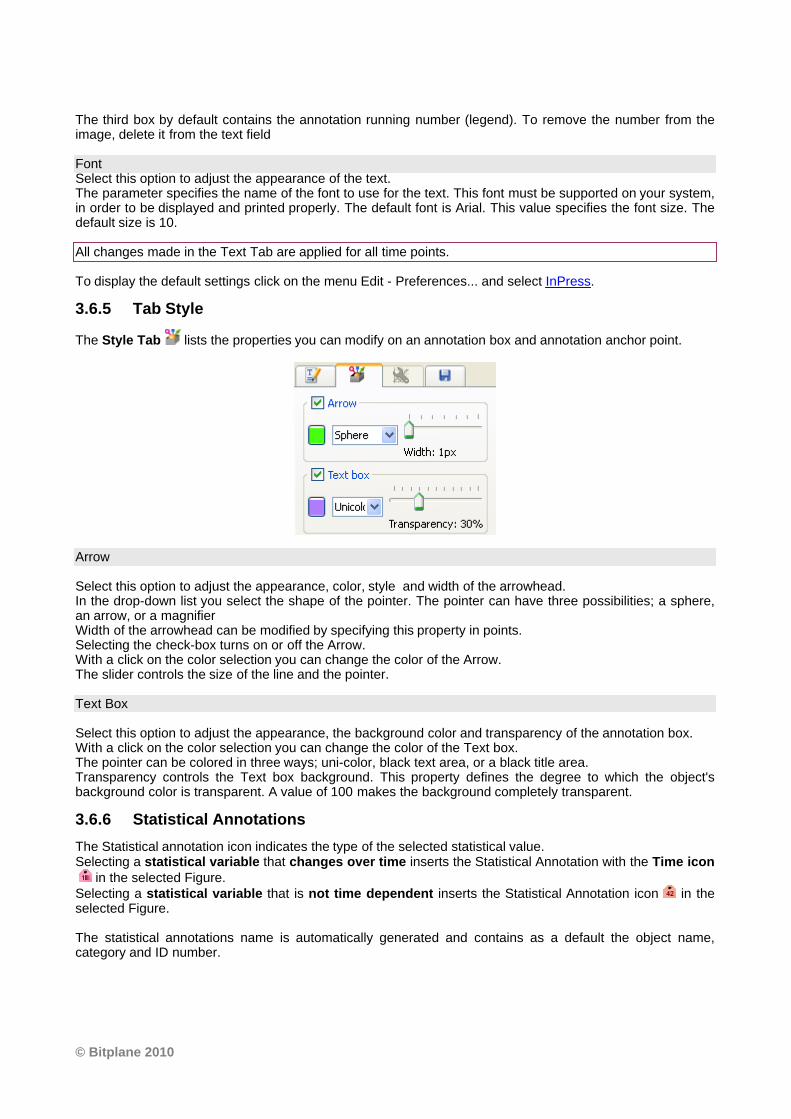
3.6.5 Tab Style
The Style Tab lists the properties you can modify on an annotation box and annotation anchor point.
Arrow
Select this option to adjust the appearance, color, style and width of the arrowhead. In the drop-down list you select the shape of the pointer. The pointer can have three possibilities; a sphere,an arrow, or a magnifierWidth of the arrowhead can be modified by specifying this property in points.Selecting the check-box turns on or off the Arrow.With a click on the color selection you can change the color of the Arrow.The slider controls the size of the line and the pointer.
Text Box
Select this option to adjust the appearance, the background color and transparency of the annotation box.With a click on the color selection you can change the color of the Text box.The pointer can be colored in three ways; uni-color, black text area, or a black title area.Transparency controls the Text box background. This property defines the degree to which the object'sbackground color is transparent. A value of 100 makes the background completely transparent.
3.6.6 Statistical Annotations
The Statistical annotation icon indicates the type of the selected statistical value.Selecting a statistical variable that changes over time inserts the Statistical Annotation with the Time icon in the selected Figure. Selecting a statistical variable that is not time dependent inserts the Statistical Annotation icon in theselected Figure.
The statistical annotations name is automatically generated and contains as a default the object name,category and ID number.
Imaris Reference Manual
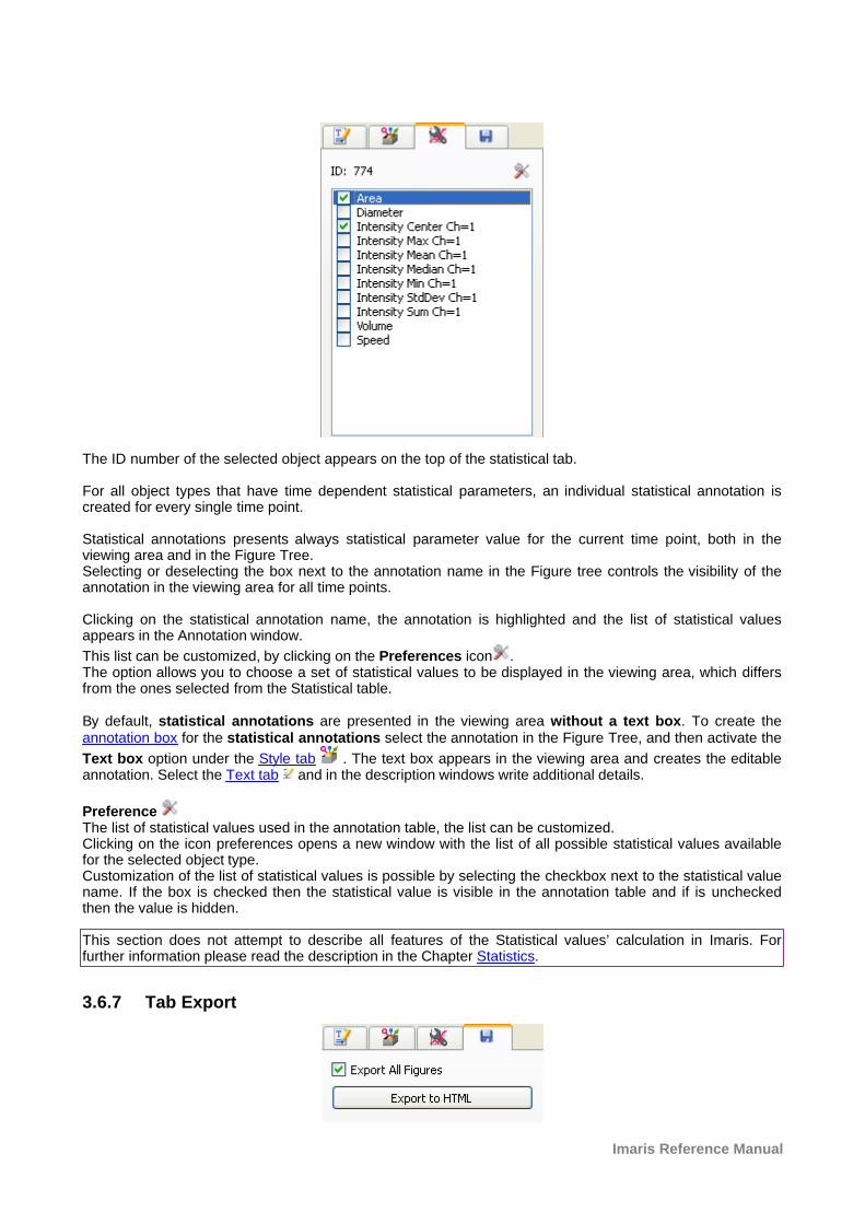
The ID number of the selected object appears on the top of the statistical tab.
For all object types that have time dependent statistical parameters, an individual statistical annotation iscreated for every single time point.
Statistical annotations presents always statistical parameter value for the current time point, both in theviewing area and in the Figure Tree. Selecting or deselecting the box next to the annotation name in the Figure tree controls the visibility of theannotation in the viewing area for all time points.
Clicking on the statistical annotation name, the annotation is highlighted and the list of statistical valuesappears in the Annotation window.
This list can be customized, by clicking on the Preferences icon .The option allows you to choose a set of statistical values to be displayed in the viewing area, which differsfrom the ones selected from the Statistical table.
By default, statistical annotations are presented in the viewing area without a text box. To create theannotation box for the statistical annotations select the annotation in the Figure Tree, and then activate the
Text box option under the Style tab . The text box appears in the viewing area and creates the editableannotation. Select the Text tab and in the description windows write additional details.
Preference The list of statistical values used in the annotation table, the list can be customized. Clicking on the icon preferences opens a new window with the list of all possible statistical values availablefor the selected object type.Customization of the list of statistical values is possible by selecting the checkbox next to the statistical valuename. If the box is checked then the statistical value is visible in the annotation table and if is uncheckedthen the value is hidden.
This section does not attempt to describe all features of the Statistical values’ calculation in Imaris. Forfurther information please read the description in the Chapter Statistics.
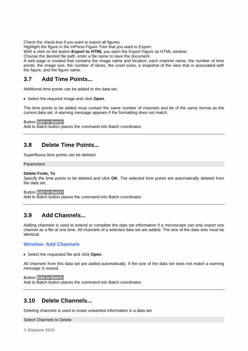
3.6.7 Tab Export
© Bitplane 2010
Check the check-box if you want to export all figures. Highlight the figure in the InPress Figure Tree that you want to Export.With a click on the button Export to HTML you open the Export Figure as HTML window.Choose the desired file path, enter a file name to save the document.A web page is created that contains the image name and location, each channel name, the number of timepoints, the image size, the number of slices, the voxel sizes, a snapshot of the view that is associated withthe figure, and the figure name.
3.7 Add Time Points...
Additional time points can be added to the data set.
· Select the required image and click Open.
The time points to be added must contain the same number of channels and be of the same format as thecurrent data set. A warning message appears if the formatting does not match.
Button Add to Batch Add to Batch button places the command into Batch coordinator.
3.8 Delete Time Points...
Superfluous time points can be deleted.
Parameters
Delete From, ToSpecify the time points to be deleted and click OK. The selected time points are automatically deleted fromthe data set.
Button Add to Batch Add to Batch button places the command into Batch coordinator.
3.9 Add Channels...
Adding channels is used to extend or complete the data set information if a microscope can only export onechannel as a file at one time. All channels of a selected data set are added. The size of the data sets must beidentical.
Window: Add Channels
· Select the requested file and click Open.
All channels from this data set are added automatically. If the size of the data set does not match a warningmessage is issued.
Button Add to Batch Add to Batch button places the command into Batch coordinator.
3.10 Delete Channels...
Deleting channels is used to erase unwanted information in a data set.
Select Channels to Delete
Imaris Reference Manual
Channel 1...nSelect the channel to be deleted in the Delete Channels box and click OK. The effect is immediately visibleon the image.
Button Add to Batch Add to Batch button places the command into Batch coordinator.
See also:Menu File - Open - Reader Configuration
3.11 Add Slices...
Adding slices may become necessary if through manipulation or during file export or formatting the data setconsists of less than the originally acquired number of slices.
Window: Add Slices
· Select the requested file and click Open.
All slices from this data set are added automatically. The x-, and y-values of the two data sets must beidentical and the same number of channels is required.
Button Add to Batch Add to Batch button places the command into Batch coordinator.
3.12 Delete Slices...
Parameters
Slice number [1...n]Specify the slice to be deleted and click OK. The slice is automatically deleted from the data set.
Button Add to Batch Add to Batch button places the command into Batch coordinator.
3.13 Crop Time...
The total number of time points can be reduced at the beginning or end of the series of images.
Parameters
From, ToEnter the time points to be included in the data set and click OK. All other time points are deleted from thedata set.
Button Add to Batch Add to Batch button places the command into Batch coordinator.
See also:Menu File - Open - Reader Configuration
© Bitplane 2010
3.14 Resample Time...
The total number of time points can be reduced to display the images at a faster speed.
Parameters
New Number of Time PointsSpecify the number of time points needed and click OK.
The process of resampling the time points takes a while. When the process is finished, the time bar displaysthe new number of time points.
Button Add to Batch Add to Batch button places the command into Batch coordinator.
See also:Menu File - Open - Reader Configuration
3.15 Crop 3D...
Cropping the data set allows you to crop the images down to the region of interest. Cropping reduces the sizeof the data set and makes it easier and faster to handle the viewing and storing of the images.
Preview
Display of a sectional view of the actual image (current time point). A rectangle, representing the region ofinterest (ROI), is overlaid on all three views.
Select Crop Dimensions
X, Y, Z, From, To, SizeModify the size and the position of the region of interest by entering the direct values in the corresponding x-,y-, and z-fields or as follows:
· To move the ROI, click inside the rectangle, hold the mouse button down & drag the entire ROI around.· To shape the ROI, click on a handle, hold the mouse button it down and reshape the ROI. Side handles
affect one direction, corner handles two directions.
The modifications apply to all slices and all time points of the image.
Click OK when finished. The data set is cut down to the marked ROI. The rest is erased.
Button Add to Batch Add to Batch button places the command into Batch coordinator.
See also:Menu File - Open - Reader Configuration
3.16 Resample 3D...
Resampling reduces the voxel density in a data set to fasten its processing. Reducing the data size alsodeteriorates the resolution. Resampling reduces the number of voxels in a grid but keeps the originalrelationship between the voxels.
New Size
X, Y, ZThe fields display the current x-, y-, and z-values. The requested values can be directly entered in the fields.
Imaris Reference Manual
Aspect Ratio
Fixed Ratio X/YFixed Ratio X/Y/ZThe Aspect Ratio of the data set’s dimensions can be kept by checking the respective Fixed Ratio options.Clicking the OK button resamples the data set to the entered values.
Use a Gaussian filter as low-pass before sampling down an image.
Button Add to Batch Add to Batch button places the command into Batch coordinator.
See also:Menu File - Open - Reader ConfigurationMenu Image Processing - Smoothing - Gaussian Filter
3.17 Change Data Type...
Type
FromDisplays the current data set type.
ToDrop-down list to select the requested data set type from the supported types:
· unsigned 8 bit for the range 0...255.· unsigned 16 bit (0...65535).· 32 bit float.
Range Adjustment
Check field to determine how the data values are translated during the change.
NoneData values are imported in the new type.
Source Range to Target Range Maximum data values are scaled to the new range (e.g., 0...255 to 0...65535).
Data Range to Target RangeActual data range values are interpolated to the new range (e.g., 0...150 to 0...65535).
Button Add to Batch Add to Batch button places the command into Batch coordinator.
3.18 Preferences...
The adjustable parameters in the preferences are application specific and Imaris stores this preferences foran individual user.
SystemDisplayLoadingCalculationTimeSurpassStatistics
© Bitplane 2010
Custom ToolsLicencesUpdateUsage Data3D CursorInPressAdvanced
3.18.1 System
Displays the basic system parameters of your Windows computer. Processor
Number of ProcessorProcessor ArchitectureProcessor SpeedInformation about the number of Processors, Processor Type and Processor Speed.
Graphics
OpenGL RendererOpenGL VersionPixel ShaderOpenGL ExtensionsInformation about the OpenGL Renderer, OpenGL Version, Pixel Shader, and OpenGL Extensions.
Operating System
OSVersion (Build)Service PackInformation about the operating system, the installed Version and the service pack.
Memory Status
Physical Memory installedPhysical Memory availableInformation about the available amount of internal memory.
Window: Hardware Settings
Data Cache
Memory LimitThe memory limit defines how much RAM memory Imaris can use before caching on the disk starts. Thevalue must stay below the total amount of installed RAM on the system to work properly. 32-bit systems cannot handle more than 2-3 GB per application.
Display
Texture Cache LimitThe texture cache limit defines how much VideoRAM, RAM Imaris can use for textures. This should be set tothe same value as the amount of VideoRAM on your graphics board.
Open GL Test The result of the open GL test displays on the right hand side.· Congratulations, your graphics board is able to display huge data.
Imaris Reference Manual
· Your graphics board is not capable of displaying huge data. Some features will be unavailable.
Button OKTo apply the changes click on OK.
Button CancelIf you do not want to save the changes click on Cancel.
3.18.2 Display
Select the viewing properties and the basic colors for the backgrounds and selection in the gallery. Display
InterpolateIf checked, the images are automatically interpolated for a smoother display.
Texture Cache Limit (MB)Before displaying any image data, Imaris converts the data into a configuration (called textures) that isoptimized by the graphics hardware. The value of the Texture Cache Limit determines how many texturescan be stored in RAM. Set the value to the memory of your graphics card.
Colors
Background ColorThe background color appears when there is no image to be displayed or when the displayed image does notfill the whole View Area.
Please note: The background color setting has not effect on the MIP mode. The default color for MIP(max) isblack and MIP(min) is white.
Button Select...Click on this button to open the color selection window to change the respective color.
Background Color 2Background marking the original position if an image is moved.
Button Select...Click on this button to open the color selection window to change the respective color.
Checkered Background for BlendingWhen using the blending mode, a checkered background displays in Full 3D blend and in Surpass.
Tile SizeAllows definition of the tile size for a checkered background.
Linear Color Progress for BlendingThe background displays a color gradient in blend progress projections and in Surpass.
Selection ColorColor of selection frame and drawing lines in contour surfaces.
Button Select...Click on this button to open the color selection window to change the respective color.
Measurement ColorColor of measurements points and lines visible in the image (in the Slice view and the Surpass view).
Button Select...
© Bitplane 2010
Click on this button to open the color selection window to change the respective color.
Coordinate Axis/Scale Bar
Show Coordinates AxisShow DateShow Scale BarShow TimeShow Scale Bar LabelShow relative Time
These options change the display of the scale bar, labels and time information in the Slice, Selection, Galleryand Surpass View. To choose the style of timestamp to be displayed select either Show Times or Show relative Time. Show Times option display the acquisition time. Show relative TimedThe option display timestamps for the image time series. The first time point is designated as time zero andall other times are displayed relative to that.
Select options to display coordinate axis, date, scale bar, scale bar label or time on screen in the ViewingArea.
Please note: To display the Coordinates Axis in the Surpass view the option Axis Labels in the Frame-TabSetting must be also selected.
Adjusting Scale BarYou can alter the length, width, location and font size of the interactive scale bar. All changes are instantlydisplayed in the viewing area.Extend or shorten the scale bar by clicking and dragging one end of it.Move the scale bar to any location in the viewing by dragging itZooming in or out of the image the scale bars are automatically updated.
Off Screen Rendering (for saving Snapshots and Movies)Check this box to save only the viewing area. For the Snapshot and Movie Imaris hides additional controlelements. If you un-check this box the actual screen display is saved, e.g. if the window Display Adjustmentsis in front of the viewing area this window is saved as well.
Show System MonitorsCheck this box to display the system monitors in the Status Bar at the bottom of the screen. The first windowdisplays the "reads per sec", the second the "writes per sec", the third the "write requests in queue" and thelast the "percentage read cache hits". These are useful information especially if you work with huge datasets.
Button OKTo apply the changes click on OK.
Button CancelIf you do not want to save the changes click on Cancel.
See also: Menu File - Snapshot
3.18.3 Loading
Allows you to select the color assignment method used when loading data sets and to define the defaultcolors. Images in Imaris format will display in the colors defined in the image file.
Take Colors from:
Default ColorsUse the default color selection to display the loaded data set. The parameter set Default Colors (see below)
Imaris Reference Manual
is available.
File Colors (color table or base color if available, otherwise default colors)Use the original color definition of the loaded data set (usually stored in a lookup table). The parameter setDefault Colors (see below) is not available.
Emission Wavelength (from file if available, otherwise default colors)Use the color according to the emitted wavelength from the file (corresponds to the appearance under themicroscope). The parameter set Default Colors (see below) is not available.
Please note that not all file formats support lookup tables and emission wavelength.
Default Colors
The parameter set Default Colors is available, if you select Default Colors in the parameter set Take Colorsfrom (see above).
First CannelSecond ChannelThird ChannelOther ChannelsDisplay of the defined color.
iQ Disk Image File
Either type in the location of the DisckInfo5.kinetic file or use the browse button to find it. Use the Browse button to find and select the DisckInfo5.kinetic file.Open iQ files’ Clicking on the ‘Open iQ files’ opens the Image Selection window with a list of images and imageinformation. Check the box Thumbnail Preview to activate an image preview.Select the required image and click on the OK button. This will instantly create a 3D volume rendered image of the selected data set.
Browse ButtonUse the Browse button to find and select the DisckInfo5.kinetic file.
Select... ButtonClick on this button to open the color selection window to change the respective color.
OK Button To apply the changes click on OK.
Button CancelIf you do not want to save the changes click on Cancel.
3.18.4 Calculation
Calculation
Number of ProcessorsSpecify the number of processors used in calculations. See maximum number of available processors in theSystem box.
Image Processing History
Maximum Number of Commands in HistoryDefines the maximum number of operations that can be undone/redone.
Please note: Each level of image processing requires an additional copy of the full image in memory. If your

© Bitplane 2010
machine runs out of memory, set Maximum Number of Commands in History to 1.
Data Cache
Imaris uses a data caching mechanism that allows you to process images that are significantly larger thanthe physical memory (RAM) installed in the computer system. This mechanism writes image data blocks tothe disk and reads them back into the physical memory when they are needed.
Memory Limit (MB)The value of data cache limit controls the amount of data blocks Imaris will keep in memory at any time.Enter a value based on the following table.
PC32 bit Physical memory installed x 0,5; but not higher than 1.2 GB64 bit Physical memory installed x 0,5
Mac32 bit Physical memory installed x 0,5; but not higher than 2 GB
Button ApplyPress this button to apply the changes.
Cache File Paths:Imaris utilize advanced cashing when working with large images. Cache File Paths display of the paths tothe temporary files (Scratch-disks).
Please note: Setting the Cache File location to a otherwise not used disc, improves the performance whenworking on larger images. This benefits a lot from a fast SSD with minimum size 10 times the biggest datasetwhich will be used.
Button AddButton RemoveYou can use the buttons to add or remove file paths in the list.
Button OKTo apply the changes click on OK.
Button CancelIf you do not want to save the changes click on Cancel.
3.18.5 Time
These are the default parameter settings for the Time Bar.
Play Back
Specify the play back mode for the Time Bar.
Play One TimeAll time points of the data set are shown one time. The play back stops when the last time point is reached.
Repeat ForeverOnce the play back has reached the last time point, it starts at the first time point again (never ending).
Swing Back and Forth ForeverWhen the last time point is reached, the time sequence is shown in reverse until the first time point isreached.
Frame Rate: ... Frames per Second
Imaris Reference Manual
You can further specify the frame rate, i.e. the number of frames per second.
Button OKTo apply the changes click on OK.
Button CancelIf you do not want to save the changes click on Cancel.
See also:Toolbars - Time Bar
3.18.6 Surpass
Object Creation Buttons
Check the icons to be displayed on the Objects toolbar in the Surpass View.
Button Move UpButton Move DownHighlight an icon and click Move Up or Move Down to define the order of the icons in the Objects toolbar.
Key Frame Interpolation
Object Rotation Center (optimizing default user interaction)This is the default parameter, select Object Rotation Center to create a rotated animation. The distance fromthe camera to the object rotation center is always the same.
Camera Rotation Center (optimizing fly through animation)Select Camera Rotation Center to create a fly through animation. The distance from camera to object isalways the same, the rotation is not around a fixed rotation center.
Key Frame Animation
Specify the play back mode for the Key Frame Animation.
Play One TimeAll time points of the data set are shown one time. The play back stops when the last time point is reached.
Repeat ForeverOnce the play back has reached the last time point, it starts at the first time point again (never ending).
Frame Rate ... Frames per SecondYou can further specify the frame rate, i.e. the number of frames per second.
Button OKTo apply the changes click on OK.
Button CancelIf you do not want to save the changes click on Cancel.
See also:Surpass View - Overview - Surpass Tree (Objects toolbar)
3.18.7 Statistics
Show Statistic Values
The most desired set of statistics values can be specified (for display, export to MS Excel, or sorting). Checkthe values to be displayed when you open the tab Statistics in the Surpass View.

© Bitplane 2010
Show AllCheck this box and all statistical values are selected. Un-check the box and all statistical values areun-selected.
For details please refer to the respective chapter:
Menu Edit - Preferences ... - Statistics - CellMenu Edit - Preferences ... - Statistics - FilamentMenu Edit - Preferences ... - Statistics - Measurement PointsMenu Edit - Preferences ... - Statistics - SpotsMenu Edit - Preferences ... - Statistics - SurfacesMenu Edit - Preferences ... - Statistics - Volume
Button OKTo apply the changes click on OK.
Button CancelIf you do not want to save the changes click on Cancel.
See also:Surpass View - Overview - Properties Area (Tab Statistics)Coloc - Volume Statistics
3.18.7.1 Cells Statistics
ImarisCell is an Imaris module that performs automated 2D and 3D time-resolved cell image analysis. Itextracts a full spectrum of relevant information, present in the dataset, which provides a wide range ofoptions to analyze 3D and 4D image data.ImarisCell detects some features that are not easily detected by a human observer, which can lead to thecorrelation of potential important and otherwise missed variations in the cell structure and function.Cells statistics are automatically computed for each Cell object.
Show Statistic Values - Cell
Cells- Cell Acceleration Acceleration is the change in the Cell velocity over time.
Cells -Cell AreaThe sum of the surface triangles forming the Cell object.
Cells - Cell Center of Homogeneous Mass XCells - Cell Center of Homogeneous Mass YCells - Cell Center of Homogeneous Mass ZThe voxel intensity values are taken to be the ‘mass’ of each voxel.The Center of Mass is a point in which it is possible to replace the entire mass of object with a point massthat is equal to the objects mass.The Center of Image Mass is calculated by considering the equal voxel intensity distribution of all channels.
R : center of homogeneous mass (x y z)ri : center of a voxel (xi yi zi)
n : number of i Î Cell
Cells - Cell Center of Image Mass X Cells - Cell Center of Image Mass YCells - Cell Center of Image Mass Z
Imaris Reference Manual
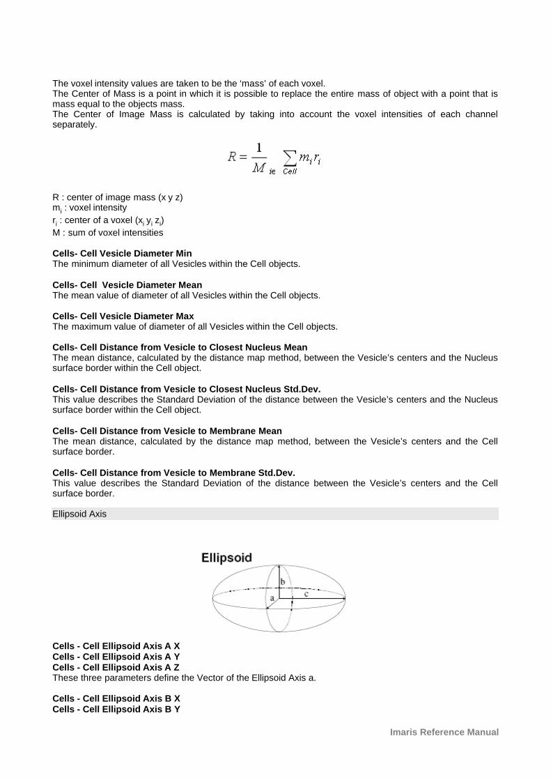
The voxel intensity values are taken to be the ‘mass’ of each voxel.The Center of Mass is a point in which it is possible to replace the entire mass of object with a point that ismass equal to the objects mass.The Center of Image Mass is calculated by taking into account the voxel intensities of each channelseparately.
R : center of image mass (x y z)mi : voxel intensity
ri : center of a voxel (xi yi zi)
M : sum of voxel intensities
Cells- Cell Vesicle Diameter Min The minimum diameter of all Vesicles within the Cell objects.
Cells- Cell Vesicle Diameter MeanThe mean value of diameter of all Vesicles within the Cell objects.
Cells- Cell Vesicle Diameter Max The maximum value of diameter of all Vesicles within the Cell objects.
Cells- Cell Distance from Vesicle to Closest Nucleus MeanThe mean distance, calculated by the distance map method, between the Vesicle’s centers and the Nucleussurface border within the Cell object.
Cells- Cell Distance from Vesicle to Closest Nucleus Std.Dev.This value describes the Standard Deviation of the distance between the Vesicle’s centers and the Nucleussurface border within the Cell object.
Cells- Cell Distance from Vesicle to Membrane MeanThe mean distance, calculated by the distance map method, between the Vesicle’s centers and the Cellsurface border.
Cells- Cell Distance from Vesicle to Membrane Std.Dev.This value describes the Standard Deviation of the distance between the Vesicle’s centers and the Cellsurface border.
Ellipsoid Axis
Cells - Cell Ellipsoid Axis A XCells - Cell Ellipsoid Axis A YCells - Cell Ellipsoid Axis A ZThese three parameters define the Vector of the Ellipsoid Axis a.
Cells - Cell Ellipsoid Axis B XCells - Cell Ellipsoid Axis B Y
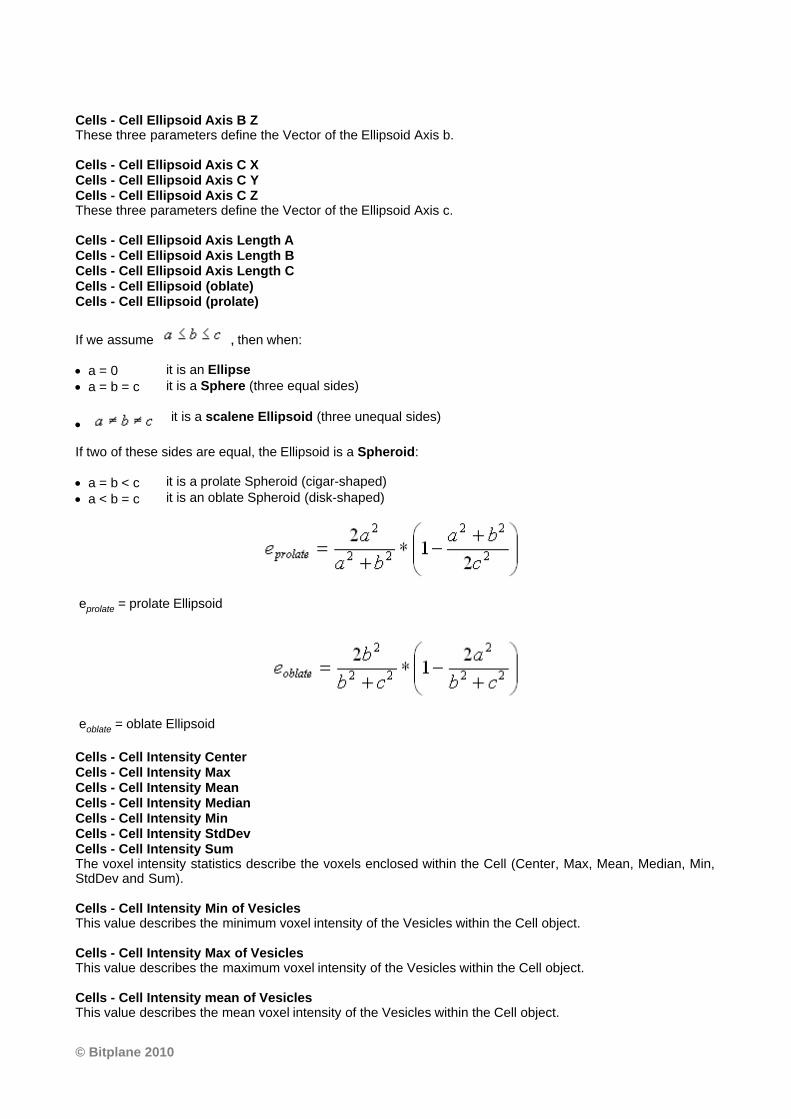
© Bitplane 2010
Cells - Cell Ellipsoid Axis B ZThese three parameters define the Vector of the Ellipsoid Axis b.
Cells - Cell Ellipsoid Axis C XCells - Cell Ellipsoid Axis C YCells - Cell Ellipsoid Axis C ZThese three parameters define the Vector of the Ellipsoid Axis c.
Cells - Cell Ellipsoid Axis Length ACells - Cell Ellipsoid Axis Length BCells - Cell Ellipsoid Axis Length CCells - Cell Ellipsoid (oblate)Cells - Cell Ellipsoid (prolate)
If we assume , then when:
· a = 0 it is an Ellipse
· a = b = c it is a Sphere (three equal sides)
·it is a scalene Ellipsoid (three unequal sides)
If two of these sides are equal, the Ellipsoid is a Spheroid:
· a = b < c it is a prolate Spheroid (cigar-shaped)
· a < b = c it is an oblate Spheroid (disk-shaped)
eprolate = prolate Ellipsoid
eoblate = oblate Ellipsoid
Cells - Cell Intensity CenterCells - Cell Intensity MaxCells - Cell Intensity MeanCells - Cell Intensity MedianCells - Cell Intensity MinCells - Cell Intensity StdDevCells - Cell Intensity SumThe voxel intensity statistics describe the voxels enclosed within the Cell (Center, Max, Mean, Median, Min,StdDev and Sum).
Cells - Cell Intensity Min of VesiclesThis value describes the minimum voxel intensity of the Vesicles within the Cell object.
Cells - Cell Intensity Max of VesiclesThis value describes the maximum voxel intensity of the Vesicles within the Cell object.
Cells - Cell Intensity mean of VesiclesThis value describes the mean voxel intensity of the Vesicles within the Cell object.
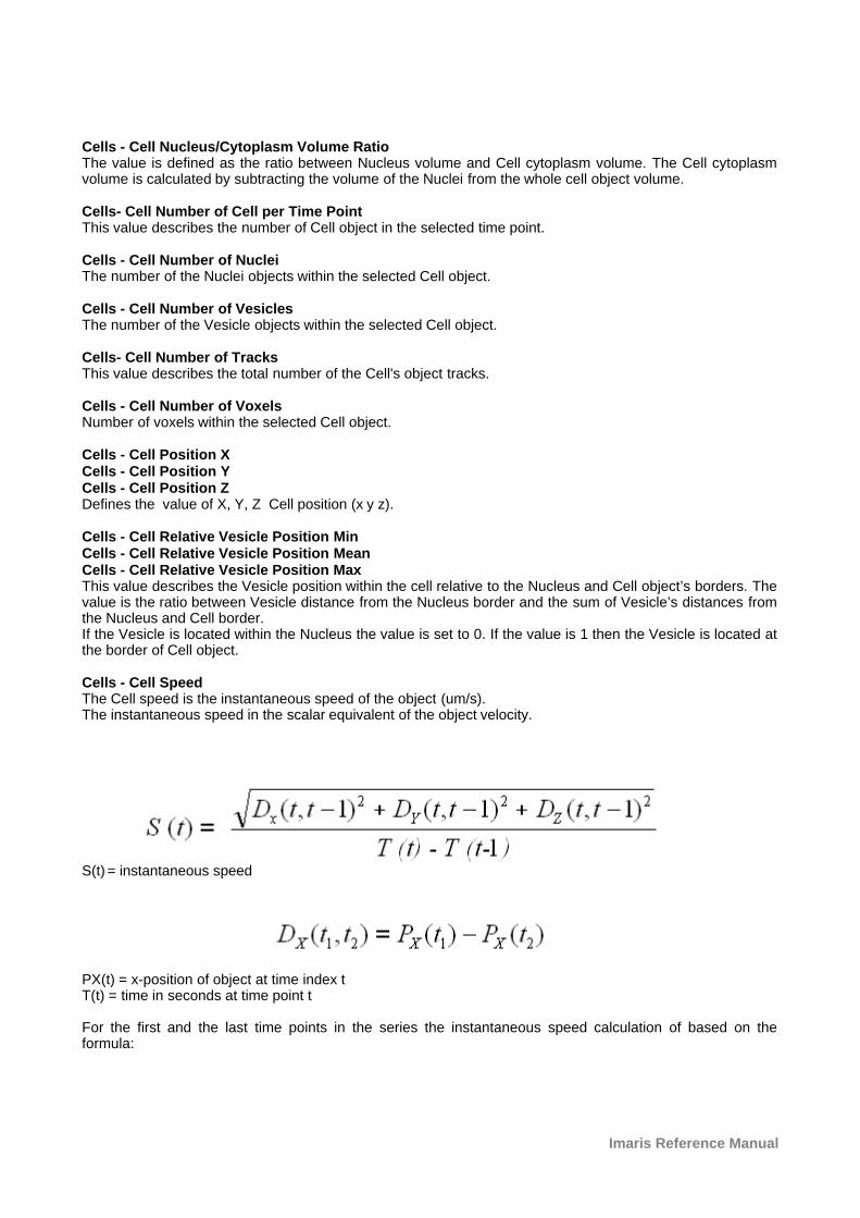
Imaris Reference Manual
Cells - Cell Nucleus/Cytoplasm Volume RatioThe value is defined as the ratio between Nucleus volume and Cell cytoplasm volume. The Cell cytoplasmvolume is calculated by subtracting the volume of the Nuclei from the whole cell object volume.
Cells- Cell Number of Cell per Time PointThis value describes the number of Cell object in the selected time point.
Cells - Cell Number of NucleiThe number of the Nuclei objects within the selected Cell object.
Cells - Cell Number of VesiclesThe number of the Vesicle objects within the selected Cell object.
Cells- Cell Number of TracksThis value describes the total number of the Cell's object tracks.
Cells - Cell Number of VoxelsNumber of voxels within the selected Cell object.
Cells - Cell Position XCells - Cell Position YCells - Cell Position ZDefines the value of X, Y, Z Cell position (x y z).
Cells - Cell Relative Vesicle Position MinCells - Cell Relative Vesicle Position MeanCells - Cell Relative Vesicle Position MaxThis value describes the Vesicle position within the cell relative to the Nucleus and Cell object’s borders. Thevalue is the ratio between Vesicle distance from the Nucleus border and the sum of Vesicle’s distances fromthe Nucleus and Cell border. If the Vesicle is located within the Nucleus the value is set to 0. If the value is 1 then the Vesicle is located atthe border of Cell object.
Cells - Cell SpeedThe Cell speed is the instantaneous speed of the object (um/s).The instantaneous speed in the scalar equivalent of the object velocity.
S(t) = instantaneous speed
PX(t) = x-position of object at time index tT(t) = time in seconds at time point t
For the first and the last time points in the series the instantaneous speed calculation of based on theformula:
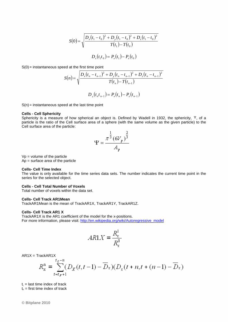
© Bitplane 2010
( )( ) ( ) ( )
( ) ( )01
2
01
2
01
2
010
tTtT
ttDttDttDS
zyx
-
-+-+-=
( ) ( ) ( )0101 tPtPttD xxx -=
S(0) = instantaneous speed at the first time point
( )( ) ( ) ( )
( ) ( )1
2
1
2
1
2
1
-
---
-
-+-+-=
nn
nnznnynnx
tTtT
ttDttDttDnS
( ) ( ) ( )11 -- -= nxnxnnxtPtPttD
S(n) = instantaneous speed at the last time point
Cells - Cell SphericitySphericity is a measure of how spherical an object is. Defined by Wadell in 1932, the sphericity, , of aparticle is the ratio of the Cell surface area of a sphere (with the same volume as the given particle) to theCell surface area of the particle:
Vp = volume of the particle Ap = surface area of the particle
Cells- Cell Time IndexThe value is only available for the time series data sets. The number indicates the current time point in theseries for the selected object.
Cells - Cell Total Number of VoxelsTotal number of voxels within the data set.
Cells- Cell Track AR1MeanTrackAR1Mean is the mean of TrackAR1X, TrackAR1Y, TrackAR1Z.
Cells- Cell Track AR1 XTrackAR1X is the AR1 coefficient of the model for the x-positions. For more information, please visit: http://en.wikipedia.org/wiki/Autoregressive_model
AR1X = TrackAR1X
tL = last time index of tracktF = first time index of track
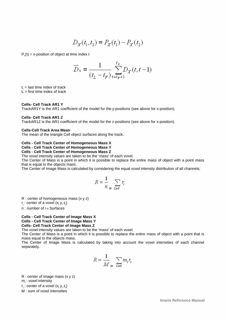
Imaris Reference Manual
PX(t) = x-position of object at time index t
tL = last time index of tracktF = first time index of track
Cells- Cell Track AR1 YTrackAR1Y is the AR1 coefficient of the model for the y-positions (see above for x-position).
Cells- Cell Track AR1 ZTrackAR1Z is the AR1 coefficient of the model for the z-positions (see above for x-position).
Cells-Cell Track Area MeanThe mean of the triangle Cell object surfaces along the track.
Cells - Cell Track Center of Homogeneous Mass XCells - Cell Track Center of Homogeneous Mass YCells - Cell Track Center of Homogeneous Mass ZThe voxel intensity values are taken to be the ‘mass’ of each voxel.The Center of Mass is a point in which it is possible to replace the entire mass of object with a point massthat is equal to the objects mass.The Center of Image Mass is calculated by considering the equal voxel intensity distribution of all channels.
R : center of homogeneous mass (x y z)ri : center of a voxel (xi yi zi)
n : number of i ÎSurfaces
Cells - Cell Track Center of Image Mass XCells - Cell Track Center of Image Mass YCells- Cell Track Center of Image Mass ZThe voxel intensity values are taken to be the ‘mass’ of each voxel.The Center of Mass is a point in which it is possible to replace the entire mass of object with a point that ismass equal to the objects mass.The Center of Image Mass is calculated by taking into account the voxel intensities of each channelseparately.
R : center of image mass (x y z)mi : voxel intensity
ri : center of a voxel (xi yi zi)
M : sum of voxel intensities
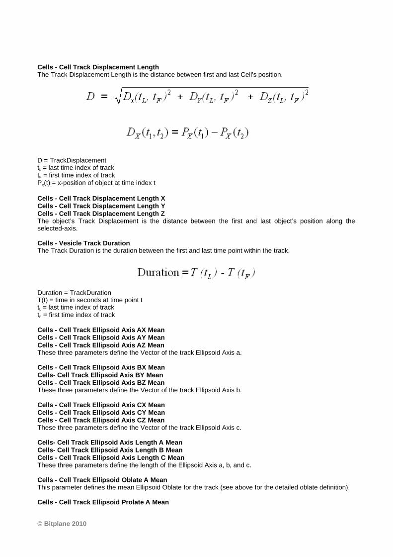
© Bitplane 2010
Cells - Cell Track Displacement LengthThe Track Displacement Length is the distance between first and last Cell's position.
D = TrackDisplacementtL = last time index of tracktF = first time index of trackPX(t) = x-position of object at time index t
Cells - Cell Track Displacement Length XCells - Cell Track Displacement Length YCells - Cell Track Displacement Length ZThe object’s Track Displacement is the distance between the first and last object’s position along theselected-axis.
Cells - Vesicle Track DurationThe Track Duration is the duration between the first and last time point within the track.
Duration = TrackDurationT(t) = time in seconds at time point ttL = last time index of tracktF = first time index of track
Cells - Cell Track Ellipsoid Axis AX MeanCells - Cell Track Ellipsoid Axis AY MeanCells - Cell Track Ellipsoid Axis AZ MeanThese three parameters define the Vector of the track Ellipsoid Axis a.
Cells - Cell Track Ellipsoid Axis BX MeanCells- Cell Track Ellipsoid Axis BY MeanCells - Cell Track Ellipsoid Axis BZ MeanThese three parameters define the Vector of the track Ellipsoid Axis b.
Cells - Cell Track Ellipsoid Axis CX MeanCells - Cell Track Ellipsoid Axis CY MeanCells - Cell Track Ellipsoid Axis CZ MeanThese three parameters define the Vector of the track Ellipsoid Axis c.
Cells- Cell Track Ellipsoid Axis Length A MeanCells- Cell Track Ellipsoid Axis Length B MeanCells - Cell Track Ellipsoid Axis Length C MeanThese three parameters define the length of the Ellipsoid Axis a, b, and c.
Cells - Cell Track Ellipsoid Oblate A MeanThis parameter defines the mean Ellipsoid Oblate for the track (see above for the detailed oblate definition).
Cells - Cell Track Ellipsoid Prolate A Mean
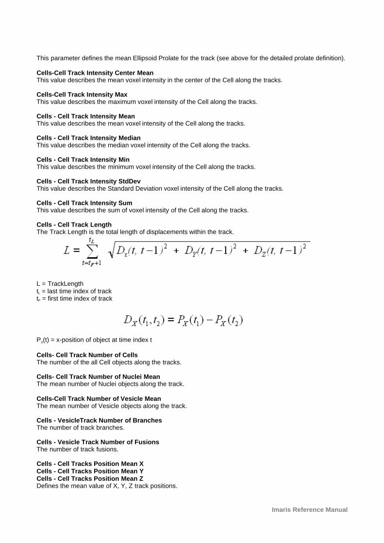
Imaris Reference Manual
This parameter defines the mean Ellipsoid Prolate for the track (see above for the detailed prolate definition).
Cells-Cell Track Intensity Center MeanThis value describes the mean voxel intensity in the center of the Cell along the tracks.
Cells-Cell Track Intensity MaxThis value describes the maximum voxel intensity of the Cell along the tracks.
Cells - Cell Track Intensity MeanThis value describes the mean voxel intensity of the Cell along the tracks.
Cells - Cell Track Intensity MedianThis value describes the median voxel intensity of the Cell along the tracks.
Cells - Cell Track Intensity MinThis value describes the minimum voxel intensity of the Cell along the tracks.
Cells - Cell Track Intensity StdDevThis value describes the Standard Deviation voxel intensity of the Cell along the tracks.
Cells - Cell Track Intensity SumThis value describes the sum of voxel intensity of the Cell along the tracks.
Cells - Cell Track LengthThe Track Length is the total length of displacements within the track.
L = TrackLengthtL = last time index of tracktF = first time index of track
PX(t) = x-position of object at time index t
Cells- Cell Track Number of CellsThe number of the all Cell objects along the tracks.
Cells- Cell Track Number of Nuclei MeanThe mean number of Nuclei objects along the track.
Cells-Cell Track Number of Vesicle MeanThe mean number of Vesicle objects along the track.
Cells - VesicleTrack Number of BranchesThe number of track branches.
Cells - Vesicle Track Number of FusionsThe number of track fusions.
Cells - Cell Tracks Position Mean XCells - Cell Tracks Position Mean YCells - Cell Tracks Position Mean ZDefines the mean value of X, Y, Z track positions.
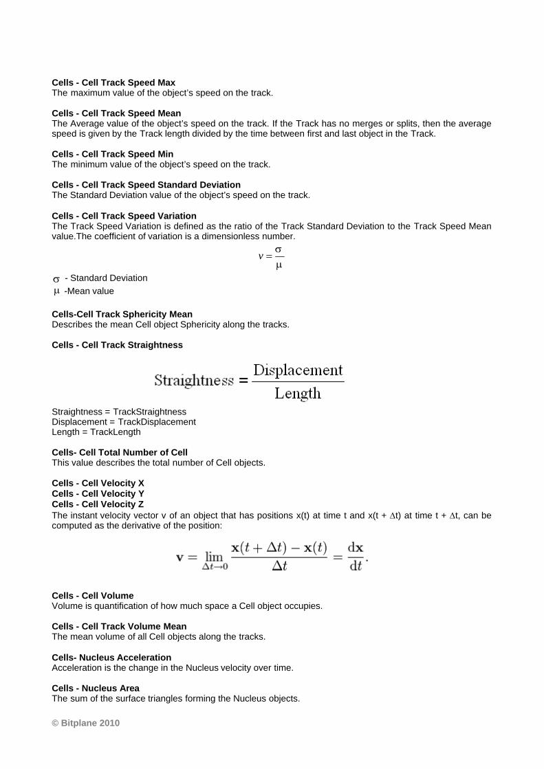
© Bitplane 2010
Cells - Cell Track Speed MaxThe maximum value of the object’s speed on the track.
Cells - Cell Track Speed Mean The Average value of the object’s speed on the track. If the Track has no merges or splits, then the averagespeed is given by the Track length divided by the time between first and last object in the Track.
Cells - Cell Track Speed MinThe minimum value of the object’s speed on the track.
Cells - Cell Track Speed Standard DeviationThe Standard Deviation value of the object’s speed on the track.
Cells - Cell Track Speed VariationThe Track Speed Variation is defined as the ratio of the Track Standard Deviation to the Track Speed Meanvalue.The coefficient of variation is a dimensionless number.
m
s=v
s - Standard Deviation
m -Mean value
Cells-Cell Track Sphericity MeanDescribes the mean Cell object Sphericity along the tracks.
Cells - Cell Track Straightness
Straightness = TrackStraightnessDisplacement = TrackDisplacementLength = TrackLength
Cells- Cell Total Number of CellThis value describes the total number of Cell objects.
Cells - Cell Velocity XCells - Cell Velocity YCells - Cell Velocity ZThe instant velocity vector v of an object that has positions x(t) at time t and x(t + Dt) at time t + Dt, can becomputed as the derivative of the position:
Cells - Cell VolumeVolume is quantification of how much space a Cell object occupies.
Cells - Cell Track Volume MeanThe mean volume of all Cell objects along the tracks.
Cells- Nucleus Acceleration Acceleration is the change in the Nucleus velocity over time.
Cells - Nucleus AreaThe sum of the surface triangles forming the Nucleus objects.
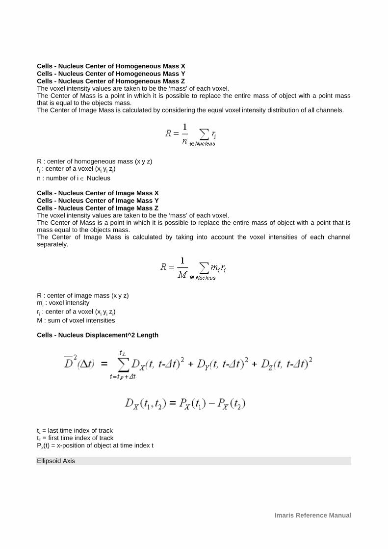
Imaris Reference Manual
Cells - Nucleus Center of Homogeneous Mass XCells - Nucleus Center of Homogeneous Mass YCells - Nucleus Center of Homogeneous Mass ZThe voxel intensity values are taken to be the ‘mass’ of each voxel.The Center of Mass is a point in which it is possible to replace the entire mass of object with a point massthat is equal to the objects mass.The Center of Image Mass is calculated by considering the equal voxel intensity distribution of all channels.
R : center of homogeneous mass (x y z)ri : center of a voxel (xi yi zi)
n : number of i Î Nucleus
Cells - Nucleus Center of Image Mass X Cells - Nucleus Center of Image Mass YCells - Nucleus Center of Image Mass ZThe voxel intensity values are taken to be the ‘mass’ of each voxel.The Center of Mass is a point in which it is possible to replace the entire mass of object with a point that ismass equal to the objects mass.The Center of Image Mass is calculated by taking into account the voxel intensities of each channelseparately.
R : center of image mass (x y z)mi : voxel intensity
ri : center of a voxel (xi yi zi)
M : sum of voxel intensities
Cells - Nucleus Displacement^2 Length
tL = last time index of tracktF = first time index of trackPX(t) = x-position of object at time index t
Ellipsoid Axis
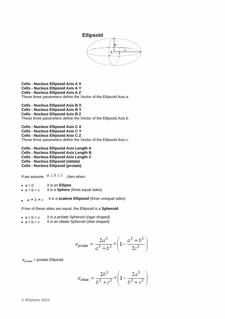
© Bitplane 2010
Cells - Nucleus Ellipsoid Axis A XCells - Nucleus Ellipsoid Axis A YCells - Nucleus Ellipsoid Axis A ZThese three parameters define the Vector of the Ellipsoid Axis a.
Cells - Nucleus Ellipsoid Axis B XCells - Nucleus Ellipsoid Axis B YCells - Nucleus Ellipsoid Axis B ZThese three parameters define the Vector of the Ellipsoid Axis b.
Cells - Nucleus Ellipsoid Axis C XCells - Nucleus Ellipsoid Axis C YCells - Nucleus Ellipsoid Axis C ZThese three parameters define the Vector of the Ellipsoid Axis c.
Cells - Nucleus Ellipsoid Axis Length ACells - Nucleus Ellipsoid Axis Length BCells - Nucleus Ellipsoid Axis Length CCells - Nucleus Ellipsoid (oblate)Cells - Nucleus Ellipsoid (prolate)
If we assume , then when:
· a = 0 it is an Ellipse
· a = b = c it is a Sphere (three equal sides)
·it is a scalene Ellipsoid (three unequal sides)
If two of these sides are equal, the Ellipsoid is a Spheroid:
· a = b < c it is a prolate Spheroid (cigar-shaped)
· a < b = c it is an oblate Spheroid (disk-shaped)
eprolate = prolate Ellipsoid
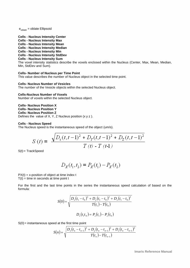
Imaris Reference Manual
eoblate = oblate Ellipsoid
Cells - Nucleus Intensity CenterCells - Nucleus Intensity MaxCells - Nucleus Intensity MeanCells - Nucleus Intensity MedianCells - Nucleus Intensity MinCells - Nucleus Intensity StdDevCells - Nucleus Intensity SumThe voxel intensity statistics describe the voxels enclosed within the Nucleus (Center, Max, Mean, Median,Min, StdDev and Sum).
Cells- Number of Nucleus per Time PointThis value describes the number of Nucleus object in the selected time point.
Cells- Nucleus Number of VesiclesThe number of the Vesicle objects within the selected Nucleus object.
Cells-Nucleus Number of VoxelsNumber of voxels within the selected Nucleus object.
Cells- Nucleus Position XCells- Nucleus Position YCells- Nucleus Position ZDefines the value of X, Y, Z Nucleus position (x y z ).
Cells - Nucleus SpeedThe Nucleus speed is the instantaneous speed of the object (um/s).
S(t) = TrackSpeed
PX(t) = x-position of object at time index tT(t) = time in seconds at time point t
For the first and the last time points in the series the instantaneous speed calculation of based on theformula:
( )( ) ( ) ( )
( ) ( )01
2
01
2
01
2
010
tTtT
ttDttDttDS
zyx
-
-+-+-=
( ) ( ) ( )0101 tPtPttD xxx -=
S(0) = instantaneous speed at the first time point
( )( ) ( ) ( )
( ) ( )1
2
1
2
1
2
1
-
---
-
-+-+-=
nn
nnznnynnx
tTtT
ttDttDttDnS
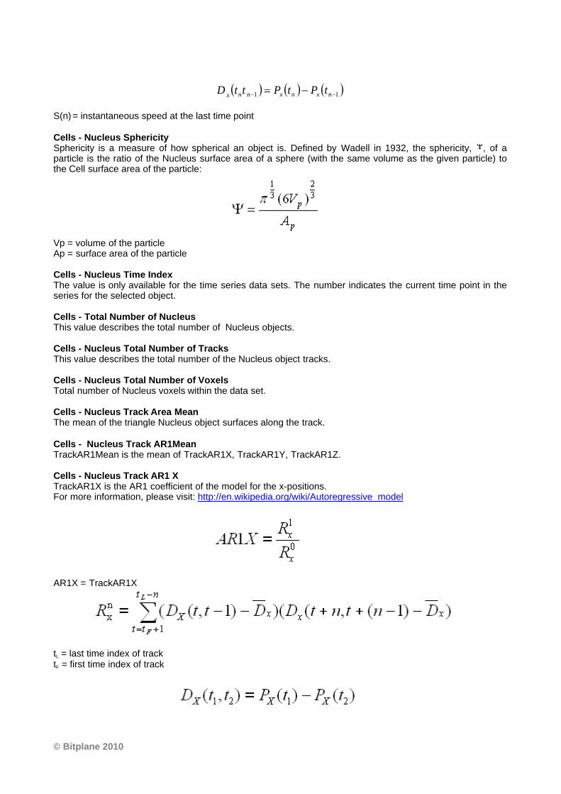
© Bitplane 2010
( ) ( ) ( )11 -- -= nxnxnnxtPtPttD
S(n) = instantaneous speed at the last time point
Cells - Nucleus SphericitySphericity is a measure of how spherical an object is. Defined by Wadell in 1932, the sphericity, , of aparticle is the ratio of the Nucleus surface area of a sphere (with the same volume as the given particle) tothe Cell surface area of the particle:
Vp = volume of the particle Ap = surface area of the particle
Cells - Nucleus Time IndexThe value is only available for the time series data sets. The number indicates the current time point in theseries for the selected object.
Cells - Total Number of NucleusThis value describes the total number of Nucleus objects.
Cells - Nucleus Total Number of TracksThis value describes the total number of the Nucleus object tracks.
Cells - Nucleus Total Number of VoxelsTotal number of Nucleus voxels within the data set.
Cells - Nucleus Track Area MeanThe mean of the triangle Nucleus object surfaces along the track.
Cells - Nucleus Track AR1MeanTrackAR1Mean is the mean of TrackAR1X, TrackAR1Y, TrackAR1Z.
Cells - Nucleus Track AR1 XTrackAR1X is the AR1 coefficient of the model for the x-positions. For more information, please visit: http://en.wikipedia.org/wiki/Autoregressive_model
AR1X = TrackAR1X
tL = last time index of tracktF = first time index of track
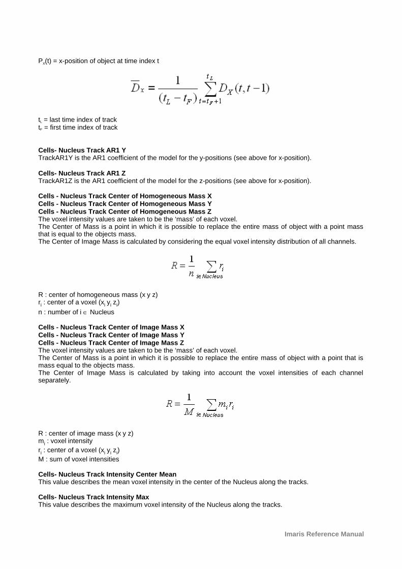
Imaris Reference Manual
PX(t) = x-position of object at time index t
tL = last time index of tracktF = first time index of track
Cells- Nucleus Track AR1 YTrackAR1Y is the AR1 coefficient of the model for the y-positions (see above for x-position).
Cells- Nucleus Track AR1 ZTrackAR1Z is the AR1 coefficient of the model for the z-positions (see above for x-position).
Cells - Nucleus Track Center of Homogeneous Mass XCells - Nucleus Track Center of Homogeneous Mass YCells - Nucleus Track Center of Homogeneous Mass ZThe voxel intensity values are taken to be the ‘mass’ of each voxel.The Center of Mass is a point in which it is possible to replace the entire mass of object with a point massthat is equal to the objects mass.The Center of Image Mass is calculated by considering the equal voxel intensity distribution of all channels.
R : center of homogeneous mass (x y z)ri : center of a voxel (xi yi zi)
n : number of i Î Nucleus
Cells - Nucleus Track Center of Image Mass XCells - Nucleus Track Center of Image Mass YCells - Nucleus Track Center of Image Mass ZThe voxel intensity values are taken to be the ‘mass’ of each voxel.The Center of Mass is a point in which it is possible to replace the entire mass of object with a point that ismass equal to the objects mass.The Center of Image Mass is calculated by taking into account the voxel intensities of each channelseparately.
R : center of image mass (x y z)mi : voxel intensity
ri : center of a voxel (xi yi zi)
M : sum of voxel intensities
Cells- Nucleus Track Intensity Center MeanThis value describes the mean voxel intensity in the center of the Nucleus along the tracks.
Cells- Nucleus Track Intensity MaxThis value describes the maximum voxel intensity of the Nucleus along the tracks.

© Bitplane 2010
Cells - Nucleus Track Intensity MeanThis value describes the mean voxel intensity of the Nucleus along the tracks.
Cells - Nucleus Track Intensity MedianThis value describes the median voxel intensity of the Nucleus along the tracks.
Cells - Nucleus Track Intensity MinThis value describes the minimum voxel intensity of the Nucleus along the tracks.
Cells - Nucleus Track Intensity StdDevThis value describes the Standard Deviation voxel intensity of the Nucleus along the tracks.
Cells - Nucleus Track Intensity SumThis value describes the sum of voxel intensity of the Nucleus along the tracks.
Cells - Nucleus Track LengthThe Track Length is the total length of displacements within the track.
L = TrackLengthtL = last time index of tracktF = first time index of track
PX(t) = x-position of object at time index t
Cells- Nucleus Track Displacement Length XCells- Nucleus Track Displacement Length YCells- Nucleus Track Displacement Length ZThe object’s Track Displacement is the distance between the first and last object’s position along theselected-axis.
Cells - Nucleus Track DurationThe Track Duration is the duration between the first and last time point within the track.
Duration = TrackDurationT(t) = time in seconds at time point ttL = last time index of tracktF = first time index of track
Cells - Nucleus Track Ellipsoid Axis AX MeanCells - Nucleus Track Ellipsoid Axis AY MeanCells - Nucleus Track Ellipsoid Axis AZ MeanThese three parameters define the Vector of the track Ellipsoid Axis a.
Cells - Nucleus Track Ellipsoid Axis BX MeanCells - Nucleus Track Ellipsoid Axis BY MeanCells - Nucleus Track Ellipsoid Axis BZ MeanThese three parameters define the Vector of the track Ellipsoid Axis b.
Imaris Reference Manual
Cells - Nucleus Track Ellipsoid Axis CX MeanCells - Nucleus Track Ellipsoid Axis CY MeanCells - Nucleus Track Ellipsoid Axis CZ MeanThese three parameters define the Vector of the track Ellipsoid Axis c.
Cells- Track Ellipsoid Axis Length A MeanCells- Track Ellipsoid Axis Length B MeanCells - Track Ellipsoid Axis Length C MeanThese three parameters define the length of the Ellipsoid Axis a, b, and c.
Cells - Nucleus Track Ellipsoid Oblate A MeanThis parameter defines the mean Ellipsoid Oblate for the track (see above for the detailed oblate definition).
Cells- Nucleus Track Ellipsoid Prolate A MeanThis parameter defines the mean Ellipsoid Prolate for the track (see above for the detailed prolate definition).
Cells - Nucleus Track Number of BranchesThe number of track branches.
Cells - Nucleus Track Number of FusionsThe number of track fusions.
Cells- Track Number of NucleusThe number of the all Nucleus objects along the tracks.
Cells - Nucleus Tracks Position Mean XCells - Nucleus Tracks Position Mean YCells - Nucleus Tracks Position Mean ZDefines the mean value of X, Y, Z Nucleus track positions.
Cells - Nucleus Track Speed MaxThe maximum value of the object’s speed on the track.
Cells - Nucleus Track Speed Mean The Average value of the object’s speed on the track. If the Track has no merges or splits, then the averagespeed is given by the Track length divided by the time between first and last object in the Track.
Cells - Nucleus Track Speed MinThe minimum value of the object’s speed on the track.
Cells - Nucleus Track Speed Standard DeviationThe Standard Deviation value of the object’s speed on the track.
Cells - Nucleus Track Speed VariationThe Track Speed Variation is defined as the ratio of the Track Standard Deviation to the Track Speed Meanvalue.The coefficient of variation is a dimensionless number.
m
s=v
s - Standard Deviation
m -Mean value
Cells- Nucleus Track Sphericity MeanDescribes the mean Nucleus object Sphericity along the tracks.
Cells - Nucleus Track Straightness
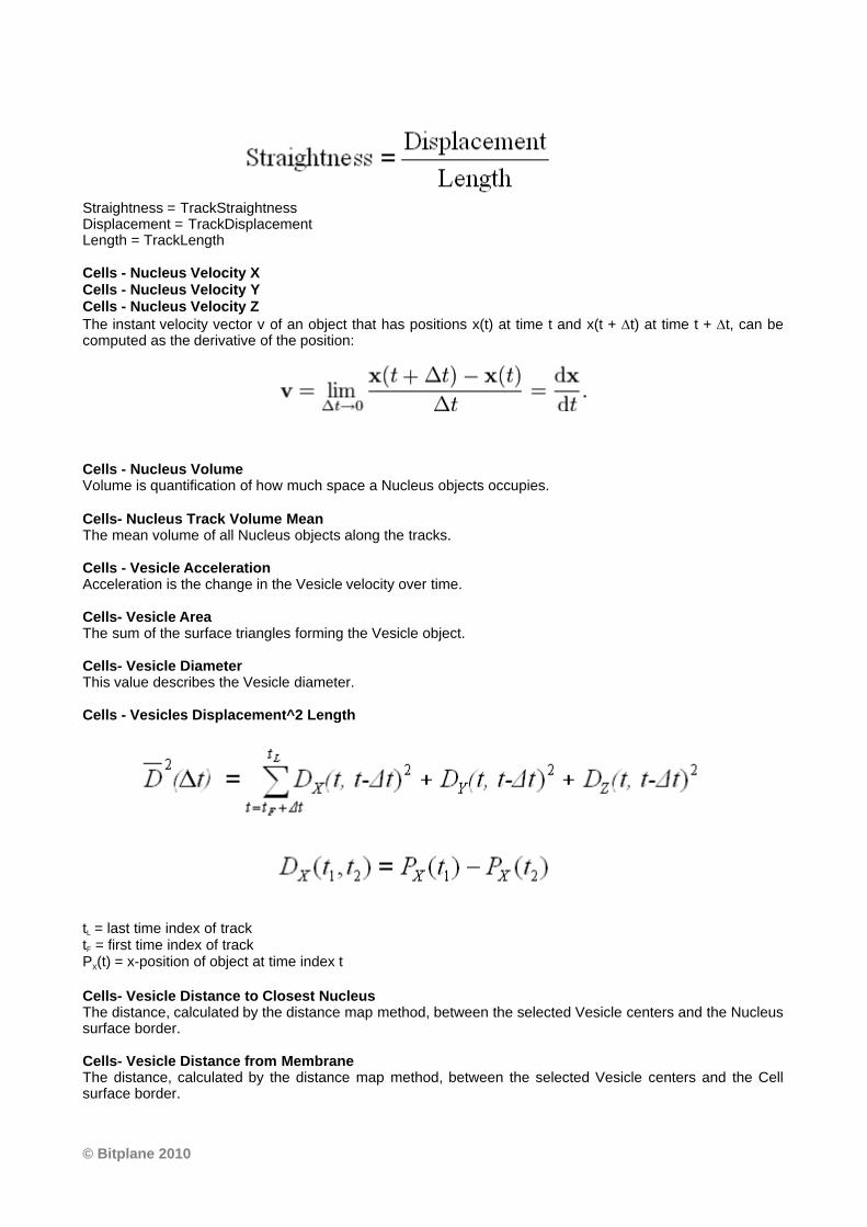
© Bitplane 2010
Straightness = TrackStraightnessDisplacement = TrackDisplacementLength = TrackLength
Cells - Nucleus Velocity XCells - Nucleus Velocity YCells - Nucleus Velocity ZThe instant velocity vector v of an object that has positions x(t) at time t and x(t + Dt) at time t + Dt, can becomputed as the derivative of the position:
Cells - Nucleus VolumeVolume is quantification of how much space a Nucleus objects occupies.
Cells- Nucleus Track Volume MeanThe mean volume of all Nucleus objects along the tracks.
Cells - Vesicle Acceleration Acceleration is the change in the Vesicle velocity over time.
Cells- Vesicle AreaThe sum of the surface triangles forming the Vesicle object.
Cells- Vesicle DiameterThis value describes the Vesicle diameter.
Cells - Vesicles Displacement^2 Length
tL = last time index of tracktF = first time index of trackPX(t) = x-position of object at time index t
Cells- Vesicle Distance to Closest NucleusThe distance, calculated by the distance map method, between the selected Vesicle centers and the Nucleussurface border.
Cells- Vesicle Distance from Membrane The distance, calculated by the distance map method, between the selected Vesicle centers and the Cellsurface border.
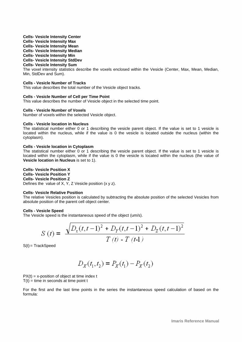
Imaris Reference Manual
Cells- Vesicle Intensity CenterCells- Vesicle Intensity MaxCells- Vesicle Intensity MeanCells- Vesicle Intensity MedianCells- Vesicle Intensity MinCells- Vesicle Intensity StdDevCells- Vesicle Intensity SumThe voxel intensity statistics describe the voxels enclosed within the Vesicle (Center, Max, Mean, Median,Min, StdDev and Sum).
Cells - Vesicle Number of TracksThis value describes the total number of the Vesicle object tracks.
Cells - Vesicle Number of Cell per Time PointThis value describes the number of Vesicle object in the selected time point.
Cells - Vesicle Number of VoxelsNumber of voxels within the selected Vesicle object.
Cells - Vesicle location in NucleusThe statistical number either 0 or 1 describing the vesicle parent object. If the value is set to 1 vesicle islocated within the nucleus, while if the value is 0 the vesicle is located outside the nucleus (within thecytoplasm).
Cells - Vesicle location in CytoplasmThe statistical number either 0 or 1 describing the vesicle parent object. If the value is set to 1 vesicle islocated within the cytoplasm, while if the value is 0 the vesicle is located within the nucleus (the value ofVesicle location in Nucleus is set to 1).
Cells- Vesicle Position XCells- Vesicle Position YCells- Vesicle Position ZDefines the value of X, Y, Z Vesicle position (x y z).
Cells- Vesicle Relative PositionThe relative Vesicles position is calculated by subtracting the absolute position of the selected Vesicles fromabsolute position of the parent cell object center.
Cells - Vesicle SpeedThe Vesicle speed is the instantaneous speed of the object (um/s).
S(t) = TrackSpeed
PX(t) = x-position of object at time index tT(t) = time in seconds at time point t
For the first and the last time points in the series the instantaneous speed calculation of based on theformula:
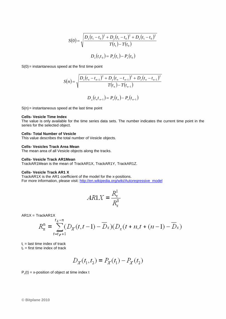
© Bitplane 2010
( )( ) ( ) ( )
( ) ( )01
2
01
2
01
2
010
tTtT
ttDttDttDS
zyx
-
-+-+-=
( ) ( ) ( )0101 tPtPttD xxx -=
S(0) = instantaneous speed at the first time point
( )( ) ( ) ( )
( ) ( )1
2
1
2
1
2
1
-
---
-
-+-+-=
nn
nnznnynnx
tTtT
ttDttDttDnS
( ) ( ) ( )11 -- -= nxnxnnxtPtPttD
S(n) = instantaneous speed at the last time point
Cells- Vesicle Time IndexThe value is only available for the time series data sets. The number indicates the current time point in theseries for the selected object.
Cells- Total Number of VesicleThis value describes the total number of Vesicle objects.
Cells- Vesicles Track Area MeanThe mean area of all Vesicle objects along the tracks.
Cells- Vesicle Track AR1MeanTrackAR1Mean is the mean of TrackAR1X, TrackAR1Y, TrackAR1Z.
Cells- Vesicle Track AR1 XTrackAR1X is the AR1 coefficient of the model for the x-positions. For more information, please visit: http://en.wikipedia.org/wiki/Autoregressive_model
AR1X = TrackAR1X
tL = last time index of tracktF = first time index of track
PX(t) = x-position of object at time index t
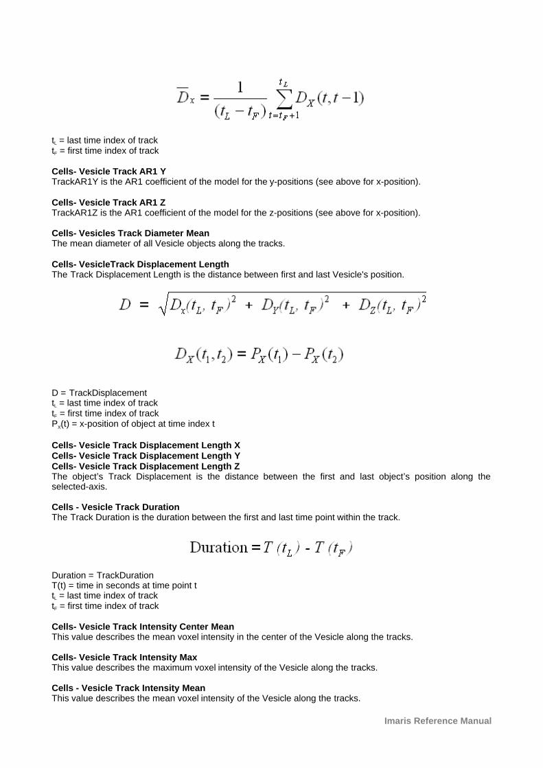
Imaris Reference Manual
tL = last time index of tracktF = first time index of track
Cells- Vesicle Track AR1 YTrackAR1Y is the AR1 coefficient of the model for the y-positions (see above for x-position).
Cells- Vesicle Track AR1 ZTrackAR1Z is the AR1 coefficient of the model for the z-positions (see above for x-position).
Cells- Vesicles Track Diameter MeanThe mean diameter of all Vesicle objects along the tracks.
Cells- VesicleTrack Displacement LengthThe Track Displacement Length is the distance between first and last Vesicle's position.
D = TrackDisplacementtL = last time index of tracktF = first time index of trackPX(t) = x-position of object at time index t
Cells- Vesicle Track Displacement Length XCells- Vesicle Track Displacement Length YCells- Vesicle Track Displacement Length ZThe object’s Track Displacement is the distance between the first and last object’s position along theselected-axis.
Cells - Vesicle Track DurationThe Track Duration is the duration between the first and last time point within the track.
Duration = TrackDurationT(t) = time in seconds at time point ttL = last time index of tracktF = first time index of track
Cells- Vesicle Track Intensity Center MeanThis value describes the mean voxel intensity in the center of the Vesicle along the tracks.
Cells- Vesicle Track Intensity MaxThis value describes the maximum voxel intensity of the Vesicle along the tracks.
Cells - Vesicle Track Intensity MeanThis value describes the mean voxel intensity of the Vesicle along the tracks.
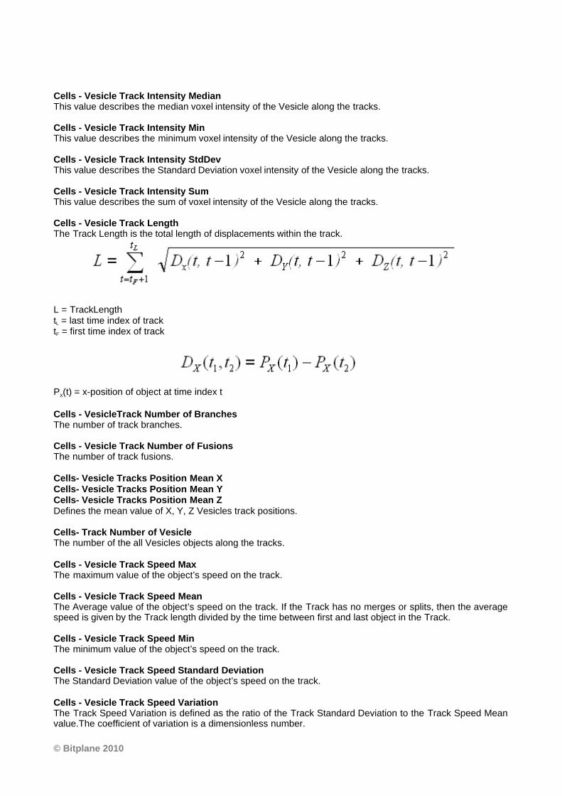
© Bitplane 2010
Cells - Vesicle Track Intensity MedianThis value describes the median voxel intensity of the Vesicle along the tracks.
Cells - Vesicle Track Intensity MinThis value describes the minimum voxel intensity of the Vesicle along the tracks.
Cells - Vesicle Track Intensity StdDevThis value describes the Standard Deviation voxel intensity of the Vesicle along the tracks.
Cells - Vesicle Track Intensity SumThis value describes the sum of voxel intensity of the Vesicle along the tracks.
Cells - Vesicle Track LengthThe Track Length is the total length of displacements within the track.
L = TrackLengthtL = last time index of tracktF = first time index of track
PX(t) = x-position of object at time index t
Cells - VesicleTrack Number of BranchesThe number of track branches.
Cells - Vesicle Track Number of FusionsThe number of track fusions.
Cells- Vesicle Tracks Position Mean XCells- Vesicle Tracks Position Mean YCells- Vesicle Tracks Position Mean ZDefines the mean value of X, Y, Z Vesicles track positions.
Cells- Track Number of VesicleThe number of the all Vesicles objects along the tracks.
Cells - Vesicle Track Speed MaxThe maximum value of the object’s speed on the track.
Cells - Vesicle Track Speed Mean The Average value of the object’s speed on the track. If the Track has no merges or splits, then the averagespeed is given by the Track length divided by the time between first and last object in the Track.
Cells - Vesicle Track Speed MinThe minimum value of the object’s speed on the track.
Cells - Vesicle Track Speed Standard DeviationThe Standard Deviation value of the object’s speed on the track.
Cells - Vesicle Track Speed VariationThe Track Speed Variation is defined as the ratio of the Track Standard Deviation to the Track Speed Meanvalue.The coefficient of variation is a dimensionless number.
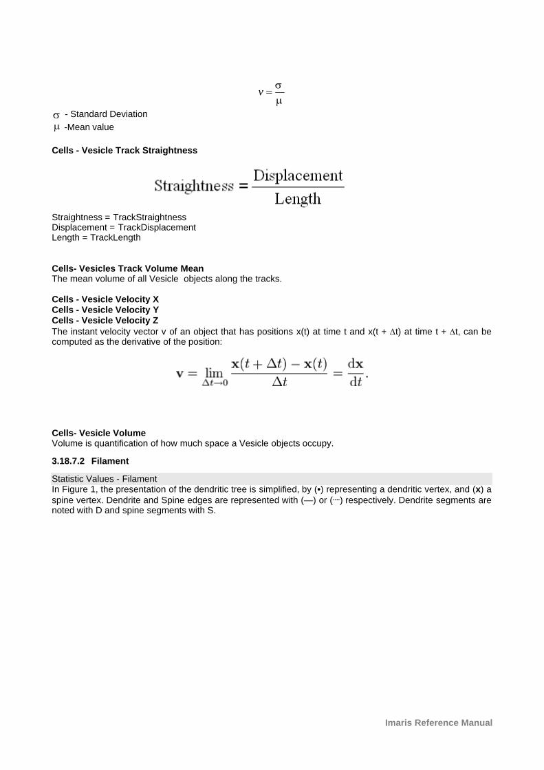
Imaris Reference Manual
m
s=v
s - Standard Deviation
m -Mean value
Cells - Vesicle Track Straightness
Straightness = TrackStraightnessDisplacement = TrackDisplacementLength = TrackLength
Cells- Vesicles Track Volume MeanThe mean volume of all Vesicle objects along the tracks.
Cells - Vesicle Velocity XCells - Vesicle Velocity YCells - Vesicle Velocity ZThe instant velocity vector v of an object that has positions x(t) at time t and x(t + Dt) at time t + Dt, can becomputed as the derivative of the position:
Cells- Vesicle Volume Volume is quantification of how much space a Vesicle objects occupy.
3.18.7.2 Filament
Statistic Values - FilamentIn Figure 1, the presentation of the dendritic tree is simplified, by (•) representing a dendritic vertex, and (x) aspine vertex. Dendrite and Spine edges are represented with (—) or (....) respectively. Dendrite segments arenoted with D and spine segments with S.
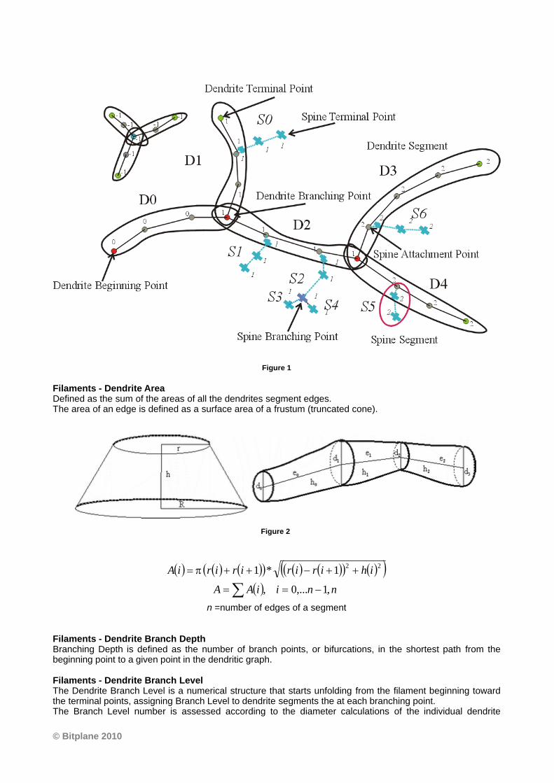
© Bitplane 2010
Figure 1
Filaments - Dendrite AreaDefined as the sum of the areas of all the dendrites segment edges.The area of an edge is defined as a surface area of a frustum (truncated cone).
Figure 2
( ) ( ) ( )( ) ( ) ( )( ) ( )( )221*1 ihiririririA ++-++= p
( ) nniiAA ,1,...0, -== å n =number of edges of a segment
Filaments - Dendrite Branch DepthBranching Depth is defined as the number of branch points, or bifurcations, in the shortest path from thebeginning point to a given point in the dendritic graph.
Filaments - Dendrite Branch LevelThe Dendrite Branch Level is a numerical structure that starts unfolding from the filament beginning towardthe terminal points, assigning Branch Level to dendrite segments the at each branching point. The Branch Level number is assessed according to the diameter calculations of the individual dendrite
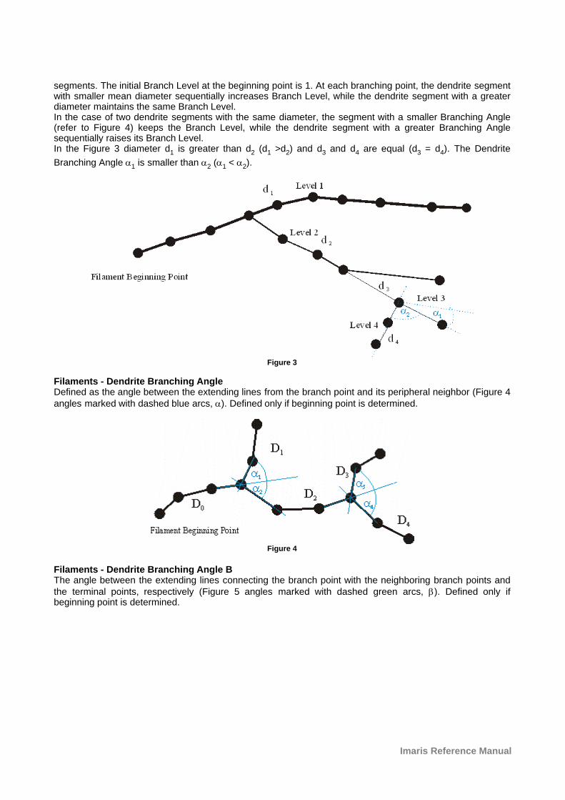
Imaris Reference Manual
segments. The initial Branch Level at the beginning point is 1. At each branching point, the dendrite segmentwith smaller mean diameter sequentially increases Branch Level, while the dendrite segment with a greaterdiameter maintains the same Branch Level. In the case of two dendrite segments with the same diameter, the segment with a smaller Branching Angle(refer to Figure 4) keeps the Branch Level, while the dendrite segment with a greater Branching Anglesequentially raises its Branch Level. In the Figure 3 diameter d1 is greater than d2 (d1 >d2) and d3 and d4 are equal (d3 = d4). The Dendrite
Branching Angle a1 is smaller than a2 (a1 < a2).
Figure 3
Filaments - Dendrite Branching AngleDefined as the angle between the extending lines from the branch point and its peripheral neighbor (Figure 4angles marked with dashed blue arcs, a). Defined only if beginning point is determined.
Figure 4
Filaments - Dendrite Branching Angle BThe angle between the extending lines connecting the branch point with the neighboring branch points andthe terminal points, respectively (Figure 5 angles marked with dashed green arcs, b). Defined only ifbeginning point is determined.
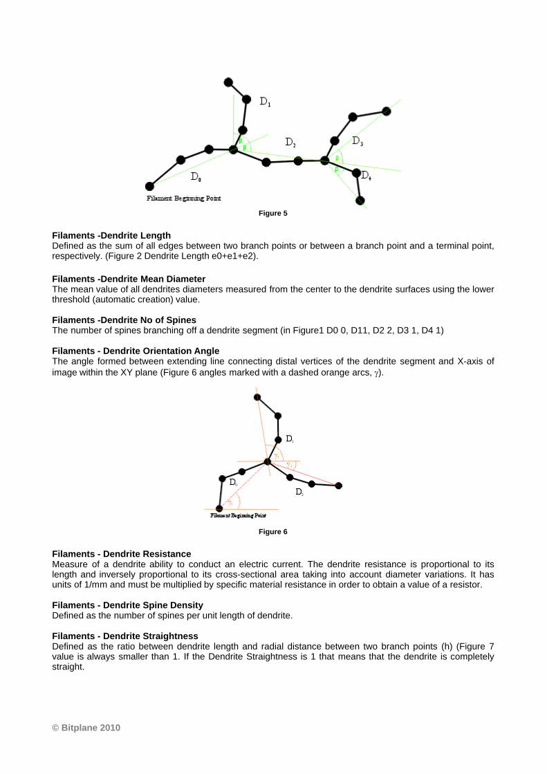
© Bitplane 2010
Figure 5
Filaments -Dendrite LengthDefined as the sum of all edges between two branch points or between a branch point and a terminal point,respectively. (Figure 2 Dendrite Length e0+e1+e2).
Filaments -Dendrite Mean Diameter The mean value of all dendrites diameters measured from the center to the dendrite surfaces using the lowerthreshold (automatic creation) value.
Filaments -Dendrite No of SpinesThe number of spines branching off a dendrite segment (in Figure1 D0 0, D11, D2 2, D3 1, D4 1)
Filaments - Dendrite Orientation AngleThe angle formed between extending line connecting distal vertices of the dendrite segment and X-axis ofimage within the XY plane (Figure 6 angles marked with a dashed orange arcs, g).
Figure 6
Filaments - Dendrite ResistanceMeasure of a dendrite ability to conduct an electric current. The dendrite resistance is proportional to itslength and inversely proportional to its cross-sectional area taking into account diameter variations. It hasunits of 1/mm and must be multiplied by specific material resistance in order to obtain a value of a resistor.
Filaments - Dendrite Spine Density Defined as the number of spines per unit length of dendrite.
Filaments - Dendrite StraightnessDefined as the ratio between dendrite length and radial distance between two branch points (h) (Figure 7value is always smaller than 1. If the Dendrite Straightness is 1 that means that the dendrite is completelystraight.
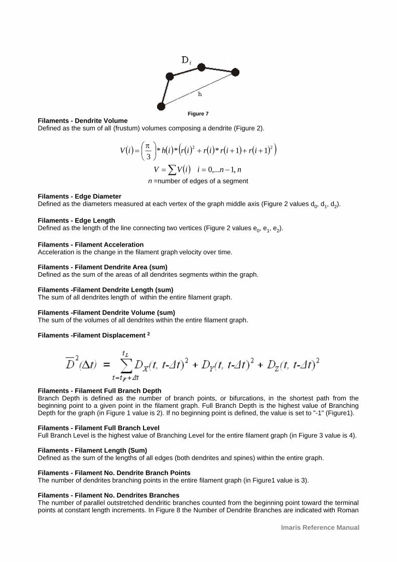
Imaris Reference Manual
Figure 7
Filaments - Dendrite Volume Defined as the sum of all (frustum) volumes composing a dendrite (Figure 2).
( ) ( ) ( ) ( ) ( ) ( )( )2211***
3++++÷
ø
öçè
æ= iririririhiV
p
( ) nniiVV ,1,...0 -== ån =number of edges of a segment
Filaments - Edge Diameter Defined as the diameters measured at each vertex of the graph middle axis (Figure 2 values d0, d1, d2).
Filaments - Edge LengthDefined as the length of the line connecting two vertices (Figure 2 values e0, e1, e2).
Filaments - Filament AccelerationAcceleration is the change in the filament graph velocity over time.
Filaments - Filament Dendrite Area (sum)Defined as the sum of the areas of all dendrites segments within the graph.
Filaments -Filament Dendrite Length (sum)The sum of all dendrites length of within the entire filament graph.
Filaments -Filament Dendrite Volume (sum)The sum of the volumes of all dendrites within the entire filament graph.
Filaments -Filament Displacement 2
Filaments - Filament Full Branch Depth Branch Depth is defined as the number of branch points, or bifurcations, in the shortest path from thebeginning point to a given point in the filament graph. Full Branch Depth is the highest value of BranchingDepth for the graph (in Figure 1 value is 2). If no beginning point is defined, the value is set to "-1" (Figure1).
Filaments - Filament Full Branch LevelFull Branch Level is the highest value of Branching Level for the entire filament graph (in Figure 3 value is 4).
Filaments - Filament Length (Sum)Defined as the sum of the lengths of all edges (both dendrites and spines) within the entire graph.
Filaments - Filament No. Dendrite Branch PointsThe number of dendrites branching points in the entire filament graph (in Figure1 value is 3).
Filaments - Filament No. Dendrites BranchesThe number of parallel outstretched dendritic branches counted from the beginning point toward the terminalpoints at constant length increments. In Figure 8 the Number of Dendrite Branches are indicated with Roman
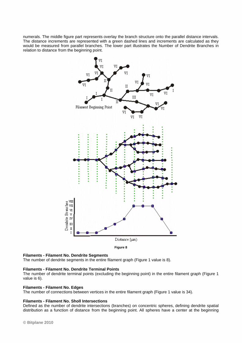
© Bitplane 2010
numerals. The middle figure part represents overlay the branch structure onto the parallel distance intervals.The distance increments are represented with a green dashed lines and increments are calculated as theywould be measured from parallel branches. The lower part illustrates the Number of Dendrite Branches inrelation to distance from the beginning point.
Figure 8
Filaments - Filament No. Dendrite SegmentsThe number of dendrite segments in the entire filament graph (Figure 1 value is 8).
Filaments - Filament No. Dendrite Terminal PointsThe number of dendrite terminal points (excluding the beginning point) in the entire filament graph (Figure 1value is 6).
Filaments - Filament No. EdgesThe number of connections between vertices in the entire filament graph (Figure 1 value is 34).
Filaments - Filament No. Sholl IntersectionsDefined as the number of dendrite intersections (branches) on concentric spheres, defining dendrite spatialdistribution as a function of distance from the beginning point. All spheres have a center at the beginning
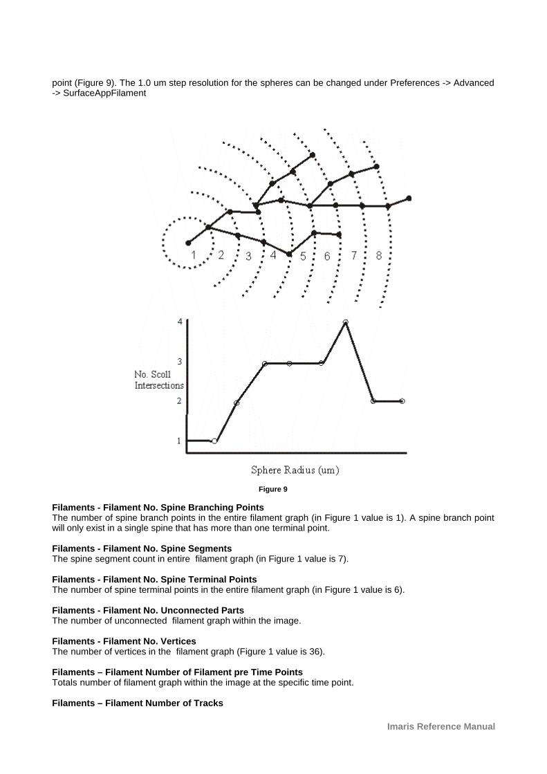
Imaris Reference Manual
point (Figure 9). The 1.0 um step resolution for the spheres can be changed under Preferences -> Advanced-> SurfaceAppFilament
Figure 9
Filaments - Filament No. Spine Branching PointsThe number of spine branch points in the entire filament graph (in Figure 1 value is 1). A spine branch pointwill only exist in a single spine that has more than one terminal point.
Filaments - Filament No. Spine SegmentsThe spine segment count in entire filament graph (in Figure 1 value is 7).
Filaments - Filament No. Spine Terminal PointsThe number of spine terminal points in the entire filament graph (in Figure 1 value is 6).
Filaments - Filament No. Unconnected PartsThe number of unconnected filament graph within the image.
Filaments - Filament No. VerticesThe number of vertices in the filament graph (Figure 1 value is 36).
Filaments – Filament Number of Filament pre Time PointsTotals number of filament graph within the image at the specific time point.
Filaments – Filament Number of Tracks
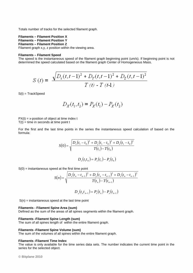
© Bitplane 2010
Totals number of tracks for the selected filament graph.
Filaments – Filament Position XFilaments – Filament Position YFilaments – Filament Position ZFilament graph x,y, z position within the viewing area.
Filaments – Filament SpeedThe speed is the instantaneous speed of the filament graph beginning point (um/s). If beginning point is notdetermined the speed calculated based on the filament graph Center of Homogeneous Mass.
S(t) = TrackSpeed
PX(t) = x-position of object at time index tT(t) = time in seconds at time point t
For the first and the last time points in the series the instantaneous speed calculation of based on theformula:
( )( ) ( ) ( )
( ) ( )01
2
01
2
01
2
010
tTtT
ttDttDttDS
zyx
-
-+-+-=
( ) ( ) ( )0101 tPtPttD xxx -=
S(0) = instantaneous speed at the first time point
( )( ) ( ) ( )
( ) ( )1
2
1
2
1
2
1
-
---
-
-+-+-=
nn
nnznnynnx
tTtT
ttDttDttDnS
( ) ( ) ( )11 -- -= nxnxnnxtPtPttD
S(n) = instantaneous speed at the last time point
Filaments - Filament Spine Area (sum)Defined as the sum of the areas of all spines segments within the filament graph.
Filaments -Filament Spine Length (sum)The sum of all spines length of within the entire filament graph.
Filaments -Filament Spine Volume (sum)The sum of the volumes of all spines within the entire filament graph.
Filaments -Filament Time IndexThe value is only available for the time series data sets. The number indicates the current time point in theseries for the selected object.
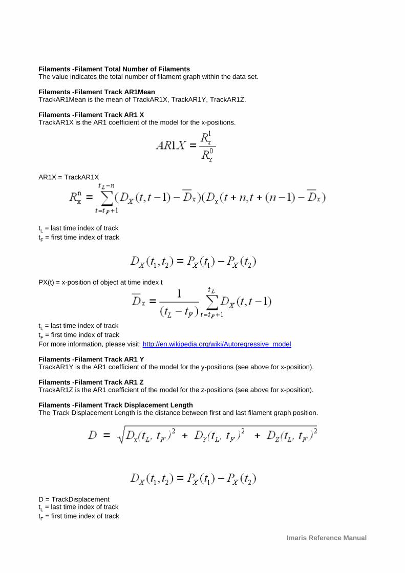
Imaris Reference Manual
Filaments -Filament Total Number of FilamentsThe value indicates the total number of filament graph within the data set.
Filaments -Filament Track AR1MeanTrackAR1Mean is the mean of TrackAR1X, TrackAR1Y, TrackAR1Z.
Filaments -Filament Track AR1 XTrackAR1X is the AR1 coefficient of the model for the x-positions.
AR1X = TrackAR1X
tL = last time index of track
tF = first time index of track
PX(t) = x-position of object at time index t
tL = last time index of track
tF = first time index of track
For more information, please visit: http://en.wikipedia.org/wiki/Autoregressive_model
Filaments -Filament Track AR1 YTrackAR1Y is the AR1 coefficient of the model for the y-positions (see above for x-position).
Filaments -Filament Track AR1 ZTrackAR1Z is the AR1 coefficient of the model for the z-positions (see above for x-position).
Filaments -Filament Track Displacement LengthThe Track Displacement Length is the distance between first and last filament graph position.
D = TrackDisplacementtL = last time index of track
tF = first time index of track
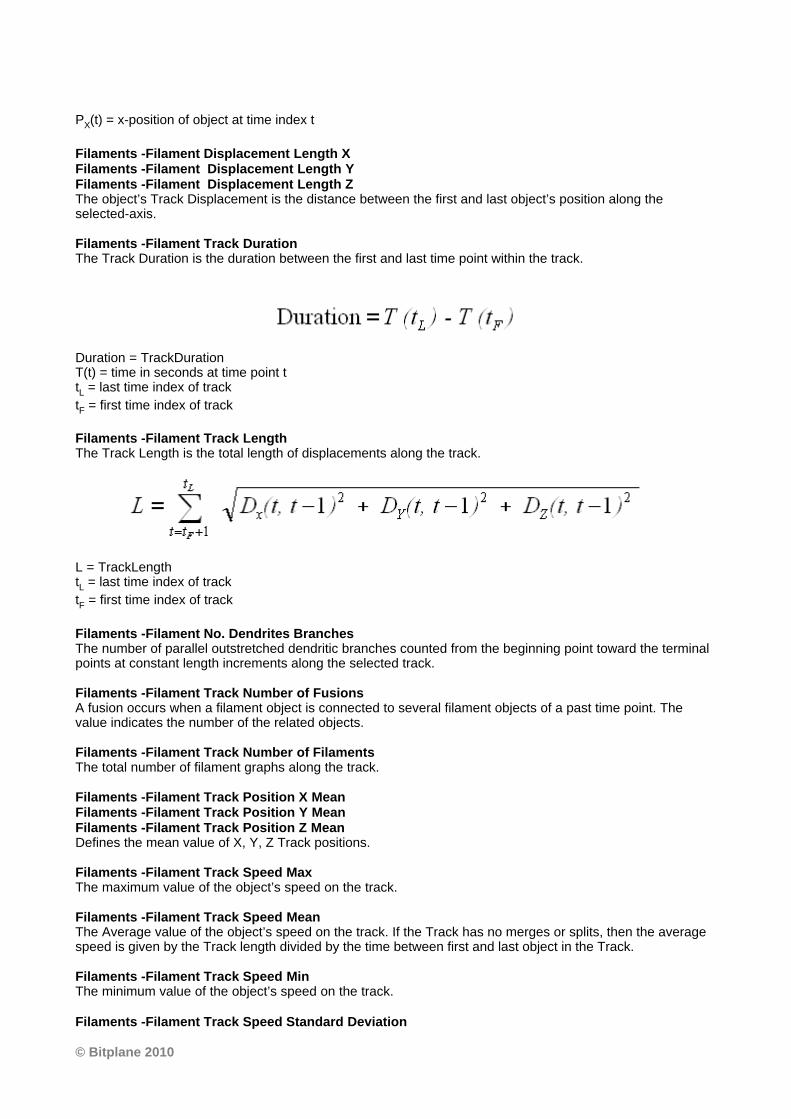
© Bitplane 2010
PX(t) = x-position of object at time index t
Filaments -Filament Displacement Length XFilaments -Filament Displacement Length YFilaments -Filament Displacement Length ZThe object’s Track Displacement is the distance between the first and last object’s position along theselected-axis.
Filaments -Filament Track DurationThe Track Duration is the duration between the first and last time point within the track.
Duration = TrackDurationT(t) = time in seconds at time point ttL = last time index of track
tF = first time index of track
Filaments -Filament Track LengthThe Track Length is the total length of displacements along the track.
L = TrackLengthtL = last time index of track
tF = first time index of track
Filaments -Filament No. Dendrites BranchesThe number of parallel outstretched dendritic branches counted from the beginning point toward the terminalpoints at constant length increments along the selected track.
Filaments -Filament Track Number of FusionsA fusion occurs when a filament object is connected to several filament objects of a past time point. Thevalue indicates the number of the related objects.
Filaments -Filament Track Number of FilamentsThe total number of filament graphs along the track.
Filaments -Filament Track Position X MeanFilaments -Filament Track Position Y MeanFilaments -Filament Track Position Z MeanDefines the mean value of X, Y, Z Track positions.
Filaments -Filament Track Speed MaxThe maximum value of the object’s speed on the track.
Filaments -Filament Track Speed MeanThe Average value of the object’s speed on the track. If the Track has no merges or splits, then the averagespeed is given by the Track length divided by the time between first and last object in the Track.
Filaments -Filament Track Speed MinThe minimum value of the object’s speed on the track.
Filaments -Filament Track Speed Standard Deviation
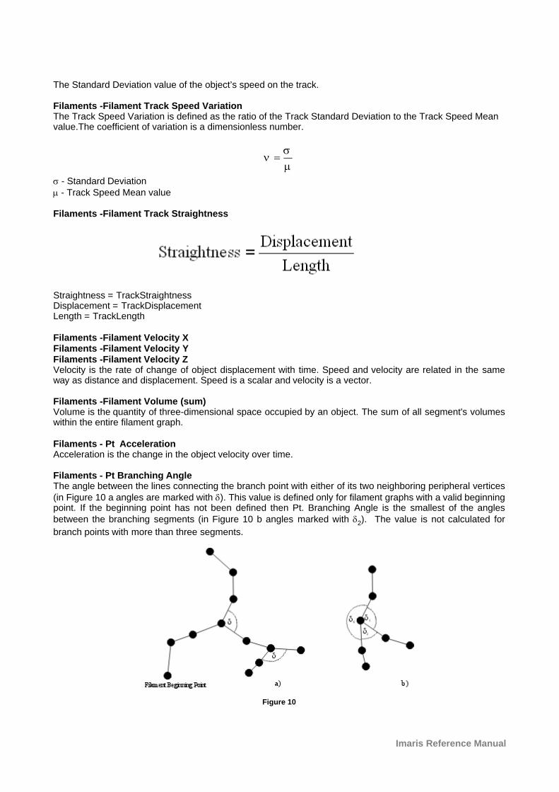
Imaris Reference Manual
The Standard Deviation value of the object’s speed on the track.
Filaments -Filament Track Speed Variation The Track Speed Variation is defined as the ratio of the Track Standard Deviation to the Track Speed Meanvalue.The coefficient of variation is a dimensionless number.
m
sn =
s - Standard Deviationm - Track Speed Mean value
Filaments -Filament Track Straightness
Straightness = TrackStraightnessDisplacement = TrackDisplacementLength = TrackLength
Filaments -Filament Velocity XFilaments -Filament Velocity YFilaments -Filament Velocity ZVelocity is the rate of change of object displacement with time. Speed and velocity are related in the sameway as distance and displacement. Speed is a scalar and velocity is a vector.
Filaments -Filament Volume (sum)Volume is the quantity of three-dimensional space occupied by an object. The sum of all segment's volumeswithin the entire filament graph.
Filaments - Pt AccelerationAcceleration is the change in the object velocity over time.
Filaments - Pt Branching Angle The angle between the lines connecting the branch point with either of its two neighboring peripheral vertices(in Figure 10 a angles are marked with d). This value is defined only for filament graphs with a valid beginningpoint. If the beginning point has not been defined then Pt. Branching Angle is the smallest of the anglesbetween the branching segments (in Figure 10 b angles marked with d2). The value is not calculated for
branch points with more than three segments.
Figure 10
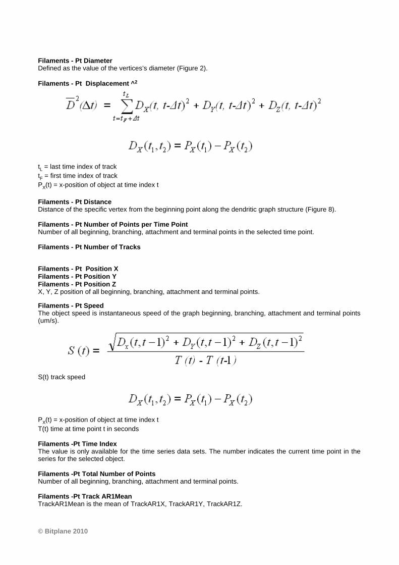
© Bitplane 2010
Filaments - Pt DiameterDefined as the value of the vertices’s diameter (Figure 2).
Filaments - Pt Displacement ^2
tL = last time index of track
tF = first time index of track
PX(t) = x-position of object at time index t
Filaments - Pt DistanceDistance of the specific vertex from the beginning point along the dendritic graph structure (Figure 8).
Filaments - Pt Number of Points per Time PointNumber of all beginning, branching, attachment and terminal points in the selected time point.
Filaments - Pt Number of Tracks
Filaments - Pt Position XFilaments - Pt Position YFilaments - Pt Position ZX, Y, Z position of all beginning, branching, attachment and terminal points.
Filaments - Pt SpeedThe object speed is instantaneous speed of the graph beginning, branching, attachment and terminal points(um/s).
S(t) track speed
PX(t) = x-position of object at time index t
T(t) time at time point t in seconds
Filaments -Pt Time IndexThe value is only available for the time series data sets. The number indicates the current time point in theseries for the selected object.
Filaments -Pt Total Number of PointsNumber of all beginning, branching, attachment and terminal points.
Filaments -Pt Track AR1MeanTrackAR1Mean is the mean of TrackAR1X, TrackAR1Y, TrackAR1Z.
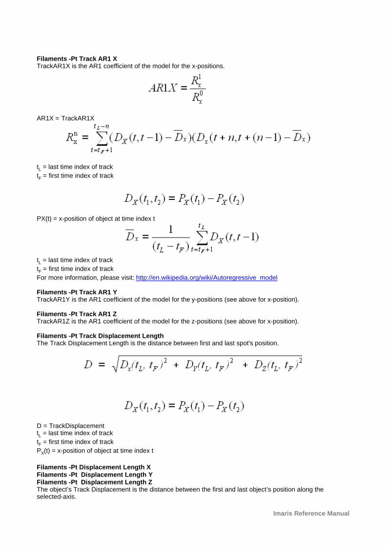
Imaris Reference Manual
Filaments -Pt Track AR1 XTrackAR1X is the AR1 coefficient of the model for the x-positions.
AR1X = TrackAR1X
tL = last time index of track
tF = first time index of track
PX(t) = x-position of object at time index t
tL = last time index of track
tF = first time index of track
For more information, please visit: http://en.wikipedia.org/wiki/Autoregressive_model
Filaments -Pt Track AR1 YTrackAR1Y is the AR1 coefficient of the model for the y-positions (see above for x-position).
Filaments -Pt Track AR1 ZTrackAR1Z is the AR1 coefficient of the model for the z-positions (see above for x-position).
Filaments -Pt Track Displacement LengthThe Track Displacement Length is the distance between first and last spot's position.
D = TrackDisplacementtL = last time index of track
tF = first time index of track
PX(t) = x-position of object at time index t
Filaments -Pt Displacement Length XFilaments -Pt Displacement Length YFilaments -Pt Displacement Length ZThe object’s Track Displacement is the distance between the first and last object’s position along theselected-axis.

© Bitplane 2010
Filaments -Pt Track DurationThe Track Duration is the duration between the first and last time point within the track.
Duration = TrackDurationT(t) = time in seconds at time point ttL = last time index of track
tF = first time index of track
Filaments -Pt Track LengthThe Track Length is the total length of displacements along the track.
L = TrackLengthtL = last time index of track
tF = first time index of track
Filaments -Pt Track No. Dendrites BranchesThe number of parallel outstretched dendritic branches counted from the beginning point toward the terminalpoints at constant length increments along the selected track.
Filaments -Pt Track Number of FusionsA fusion occurs when a filament graph beginning, branching, attachment and terminal points are connectedto several graph key points of a past time point. The value indicates the number of the related objects alongthe selected track.
Filaments -Pt Track Number of PointsThe total number of points (beginning, branching, attachment and terminal) along the track.
Filaments -Pt Track Position X MeanFilaments -Pt Track Position Y MeanFilaments -Pt Track Position Z MeanDefines the mean value of X, Y, Z Track positions.
Filaments -Pt Track Speed MaxThe maximum value of the object’s speed on the track.
Filaments -Pt Track Speed MeanThe Average value of the object’s speed on the track. If the Track has no merges or splits, then the averagespeed is given by the Track length divided by the time between first and last object in the Track.
Filaments -Pt Track Speed MinThe minimum value of the object’s speed on the track.
Filaments -Pt Track Speed Standard DeviationThe Standard Deviation value of the object’s speed on the track.
Filaments -Pt Track Speed Variation The Track Speed Variation is defined as the ratio of the Track Standard Deviation to the Track Speed Meanvalue.The coefficient of variation is a dimensionless number.
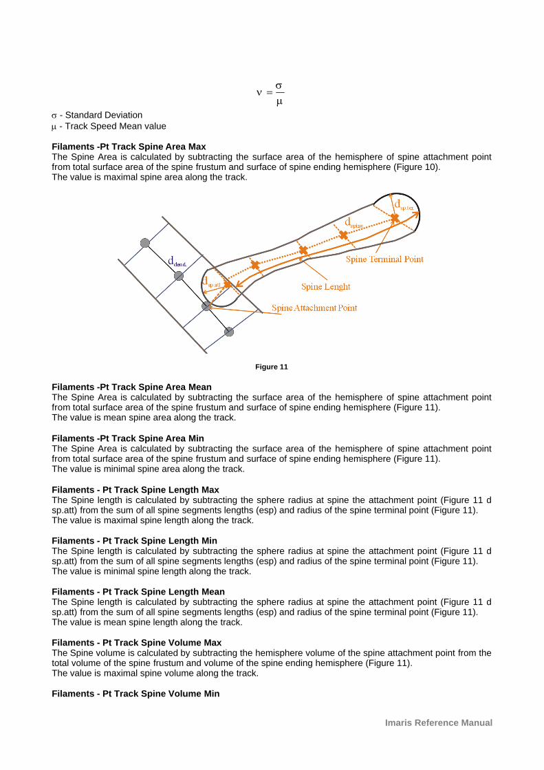
Imaris Reference Manual
m
sn =
s - Standard Deviationm - Track Speed Mean value
Filaments -Pt Track Spine Area MaxThe Spine Area is calculated by subtracting the surface area of the hemisphere of spine attachment pointfrom total surface area of the spine frustum and surface of spine ending hemisphere (Figure 10). The value is maximal spine area along the track.
Figure 11
Filaments -Pt Track Spine Area MeanThe Spine Area is calculated by subtracting the surface area of the hemisphere of spine attachment pointfrom total surface area of the spine frustum and surface of spine ending hemisphere (Figure 11). The value is mean spine area along the track.
Filaments -Pt Track Spine Area MinThe Spine Area is calculated by subtracting the surface area of the hemisphere of spine attachment pointfrom total surface area of the spine frustum and surface of spine ending hemisphere (Figure 11). The value is minimal spine area along the track.
Filaments - Pt Track Spine Length MaxThe Spine length is calculated by subtracting the sphere radius at spine the attachment point (Figure 11 dsp.att) from the sum of all spine segments lengths (esp) and radius of the spine terminal point (Figure 11).The value is maximal spine length along the track.
Filaments - Pt Track Spine Length MinThe Spine length is calculated by subtracting the sphere radius at spine the attachment point (Figure 11 dsp.att) from the sum of all spine segments lengths (esp) and radius of the spine terminal point (Figure 11).The value is minimal spine length along the track.
Filaments - Pt Track Spine Length MeanThe Spine length is calculated by subtracting the sphere radius at spine the attachment point (Figure 11 dsp.att) from the sum of all spine segments lengths (esp) and radius of the spine terminal point (Figure 11).The value is mean spine length along the track.
Filaments - Pt Track Spine Volume MaxThe Spine volume is calculated by subtracting the hemisphere volume of the spine attachment point from thetotal volume of the spine frustum and volume of the spine ending hemisphere (Figure 11).The value is maximal spine volume along the track.
Filaments - Pt Track Spine Volume Min
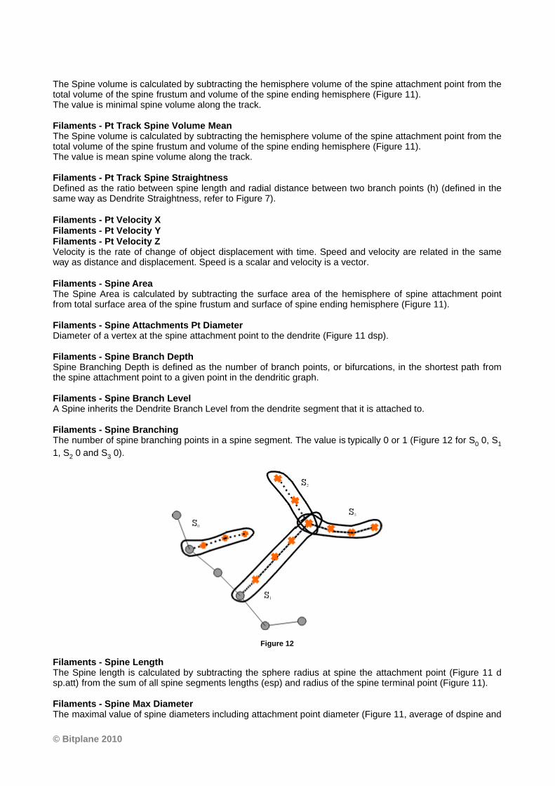
© Bitplane 2010
The Spine volume is calculated by subtracting the hemisphere volume of the spine attachment point from thetotal volume of the spine frustum and volume of the spine ending hemisphere (Figure 11).The value is minimal spine volume along the track.
Filaments - Pt Track Spine Volume MeanThe Spine volume is calculated by subtracting the hemisphere volume of the spine attachment point from thetotal volume of the spine frustum and volume of the spine ending hemisphere (Figure 11).The value is mean spine volume along the track.
Filaments - Pt Track Spine StraightnessDefined as the ratio between spine length and radial distance between two branch points (h) (defined in thesame way as Dendrite Straightness, refer to Figure 7).
Filaments - Pt Velocity XFilaments - Pt Velocity YFilaments - Pt Velocity ZVelocity is the rate of change of object displacement with time. Speed and velocity are related in the sameway as distance and displacement. Speed is a scalar and velocity is a vector.
Filaments - Spine Area The Spine Area is calculated by subtracting the surface area of the hemisphere of spine attachment pointfrom total surface area of the spine frustum and surface of spine ending hemisphere (Figure 11).
Filaments - Spine Attachments Pt DiameterDiameter of a vertex at the spine attachment point to the dendrite (Figure 11 dsp).
Filaments - Spine Branch DepthSpine Branching Depth is defined as the number of branch points, or bifurcations, in the shortest path fromthe spine attachment point to a given point in the dendritic graph.
Filaments - Spine Branch LevelA Spine inherits the Dendrite Branch Level from the dendrite segment that it is attached to.
Filaments - Spine BranchingThe number of spine branching points in a spine segment. The value is typically 0 or 1 (Figure 12 for S0 0, S1
1, S2 0 and S3 0).
Figure 12
Filaments - Spine LengthThe Spine length is calculated by subtracting the sphere radius at spine the attachment point (Figure 11 dsp.att) from the sum of all spine segments lengths (esp) and radius of the spine terminal point (Figure 11).
Filaments - Spine Max DiameterThe maximal value of spine diameters including attachment point diameter (Figure 11, average of dspine and
Imaris Reference Manual
all dsp.att ).
Filaments - Spine Min DiameterThe minimal value of spine diameters including attachment point diameter (Figure 11, average of dspine andall dsp.att ).
Filaments - Spine Mean DiameterThe mean value of spine diameters including attachment point diameter (Figure 11, average of dspine and alldsp.att ).
Filaments - Spine Neck Max DiameterFilaments - Spine Neck Mean DiameterFilaments - Spine Neck Min DiameterMaximum, Mean and Minimum value of the spine neck diameter (excluding the spine attachment andterminal pints diameters).
Filaments - Spine Neck Volume The Spine Neck volume is calculated by subtracting the volume of the spine-ending hemispheres(attachment and terminal point) from the spine volume.
Filaments - Spine Orientation AngleThe angle formed between the extending line connecting distal spine vertices in the spine segment andX-axis of the image within the XY plane (defined in the same way as Dendrite Orientation Angle, refer toFigure 6).
Filaments - Spine ResistanceMeasure of a spine's ability to conduct an electric current. The spine's resistance is proportional to its lengthand inversely proportional to its cross-sectional area taking into account the diameter variations. It has unitsof 1/um and must be multiplied by specific material resistance in order to obtain a value of resistor (defined inthe same way as Dendrite Resistance).
Filaments - Spine StraightnessDefined as the ratio between spine length and radial distance between two branch points (h) (defined in thesame way as Dendrite Straightness, refer to Figure 7).
Filaments - Spine Terminal Point DiameterDiameter of a vertex at the spine terminal point (Figure 11 dsp.ter.)
Filaments - Spine Terminal Pt Intensity CenterDefined as the intensity of the spine terminal center voxel.
Filaments -Spine Terminal Pt. VolumeSpine Terminal Pt. Volume is calculated as a volume of the sphere with the diameter of a spine terminal pointvertex (Figure 11).
Filaments - Spine VolumeThe Spine volume is calculated by subtracting the hemisphere volume of the spine attachment point from thetotal volume of the spine frustum and volume of the spine ending hemisphere (Figure 11).
See also:Surpass View - Filament - Tab Statistics
3.18.7.3 Measurement Points
Measurement Point statistics are automatically computed for each Measurement Point.
Show Statistic Values - Measurement Points
Measurement Points - DistanceDistance between the measurement points.
Measurement Points - Distance Sum
© Bitplane 2010
Sum of all measured distances.
Measurement Points - Number of PointsNumber of measurement points.
Measurement Points - Point Intensity CenterValue of the point intensity center (average) in the different channels.
Measurement Points - Point Position XPoint position in x-axis.
Measurement Points - Point Position YPoint position in y-axis.
Measurement Points - Point Position ZPoint position in z-axis.
See also:Surpass View - Measurement Points - Tab Statistics
3.18.7.4 Spots
Spots statistics are automatically computed for each Spots object. To each Spot belongs a spatial positionalong the x-, y-, and z-axis, as well as the intensity of the point it represents.
Show Statistic Values - Spots
Spots- Acceleration Acceleration is the change in the Spot(s) velocity over time.
Spots - AreaThe sum of the triangle surfaces.
Spots - DiameterThe spots diameter.
Spots - Intensity CenterIntensity of the voxel in the Spot(s) center.
Spots - Intensity MaxSpots - Intensity MeanSpots - Intensity MedianSpots - Intensity MinSpots - Intensity StdDevSpots - Intensity SumThe voxel intensity statistics describe the voxels enclosed within the Spots (Max, Mean, Median, Min, StdDevand Sum).
Spots - Number of Points per Time PointNumber of points per time point.
Spots - Number of TracksNumber of tracks.
Spots - Number of VoxelsNumber of voxels within the selected Spot objects.
Spots - Position XSpots - Position YSpots - Position ZSpots position (x y z).
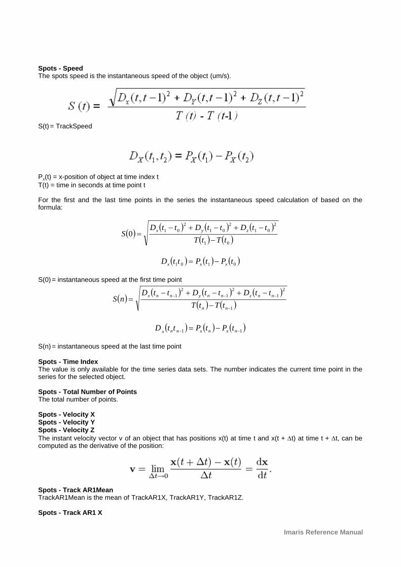
Imaris Reference Manual
Spots - SpeedThe spots speed is the instantaneous speed of the object (um/s).
S(t) = TrackSpeed
PX(t) = x-position of object at time index tT(t) = time in seconds at time point t
For the first and the last time points in the series the instantaneous speed calculation of based on theformula:
( )( ) ( ) ( )
( ) ( )01
2
01
2
01
2
010
tTtT
ttDttDttDS
zyx
-
-+-+-=
( ) ( ) ( )0101 tPtPttD xxx -=
S(0) = instantaneous speed at the first time point
( )( ) ( ) ( )
( ) ( )1
2
1
2
1
2
1
-
---
-
-+-+-=
nn
nnznnynnx
tTtT
ttDttDttDnS
( ) ( ) ( )11 -- -= nxnxnnxtPtPttD
S(n) = instantaneous speed at the last time point
Spots - Time IndexThe value is only available for the time series data sets. The number indicates the current time point in theseries for the selected object.
Spots - Total Number of PointsThe total number of points.
Spots - Velocity XSpots - Velocity YSpots - Velocity ZThe instant velocity vector v of an object that has positions x(t) at time t and x(t + Dt) at time t + Dt, can becomputed as the derivative of the position:
Spots - Track AR1MeanTrackAR1Mean is the mean of TrackAR1X, TrackAR1Y, TrackAR1Z.
Spots - Track AR1 X
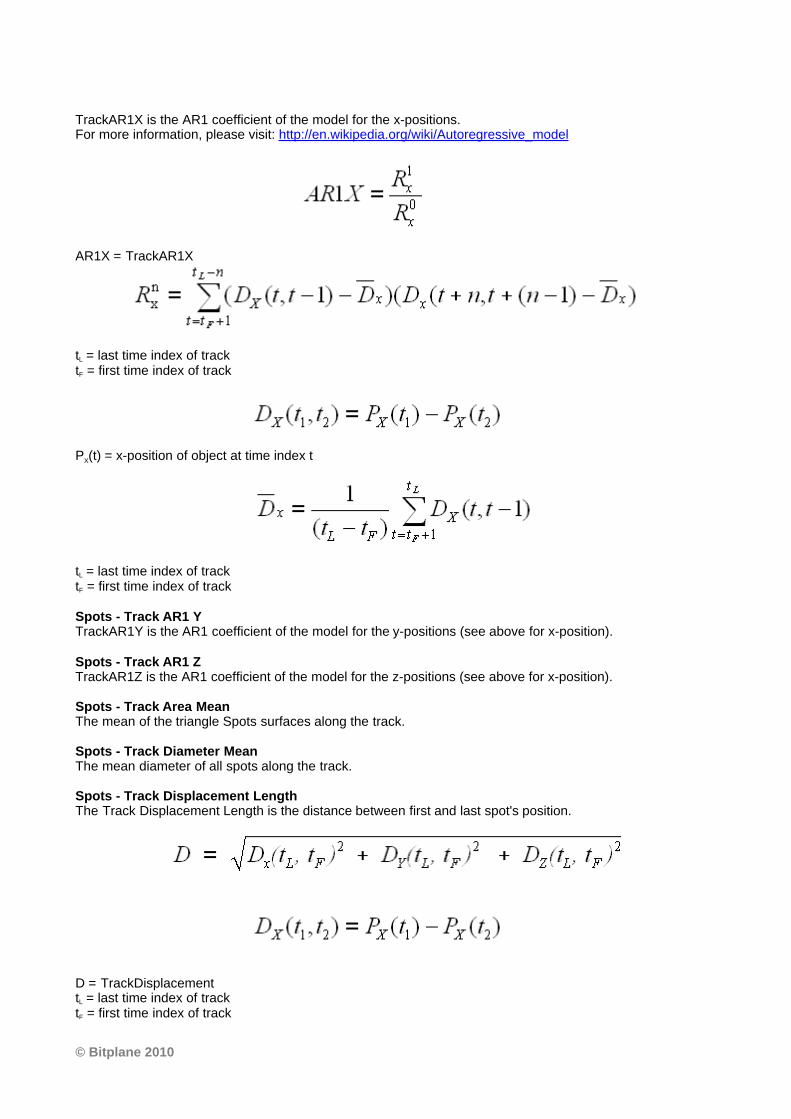
© Bitplane 2010
TrackAR1X is the AR1 coefficient of the model for the x-positions. For more information, please visit: http://en.wikipedia.org/wiki/Autoregressive_model
AR1X = TrackAR1X
tL = last time index of tracktF = first time index of track
PX(t) = x-position of object at time index t
tL = last time index of tracktF = first time index of track
Spots - Track AR1 YTrackAR1Y is the AR1 coefficient of the model for the y-positions (see above for x-position).
Spots - Track AR1 ZTrackAR1Z is the AR1 coefficient of the model for the z-positions (see above for x-position).
Spots - Track Area MeanThe mean of the triangle Spots surfaces along the track.
Spots - Track Diameter MeanThe mean diameter of all spots along the track.
Spots - Track Displacement LengthThe Track Displacement Length is the distance between first and last spot's position.
D = TrackDisplacementtL = last time index of tracktF = first time index of track

Imaris Reference Manual
PX(t) = x-position of object at time index t
Spots-Track Displacement Length XSpots-Track Displacement Length YSpots-Track Displacement Length ZThe object’s Track Displacement is the distance between the first and last object’s position along theselected-axis.
Spots - Track DurationThe Track Duration is the duration between the first and last time point within the track.
Duration = TrackDurationT(t) = time in seconds at time point ttL = last time index of tracktF = first time index of track
Spots - Track Intensity Center MeanThe mean center intensity of all spots along the track.
Spots - Track Intensity MaxThe max intensity of all spots along the track.
Spots - Track Intensity MeanThe mean intensity of all spots along the track.
Spots - Track Intensity MedianThe median track intensity of all spots along the track.
Spots - Track Intensity MinThe min track intensity of all spots along the track.
Spots - Track Intensity StdDevThe standard deviation track intensity of all spots along the track.
Spots - Track Intensity SumThe sum of the track intensity of all spots along the track. Spots - Track LengthThe Track Length is the total length of displacements within the track.
L = TrackLengthtL = last time index of tracktF = first time index of track
PX(t) = x-position of object at time index t
Spots - Track Number of BranchesThe number of track branches.
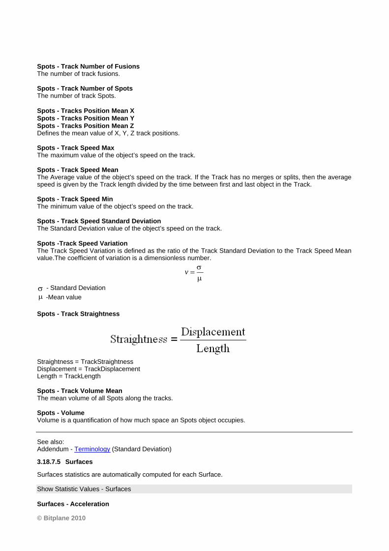
© Bitplane 2010
Spots - Track Number of FusionsThe number of track fusions.
Spots - Track Number of SpotsThe number of track Spots.
Spots - Tracks Position Mean XSpots - Tracks Position Mean YSpots - Tracks Position Mean ZDefines the mean value of X, Y, Z track positions.
Spots - Track Speed MaxThe maximum value of the object’s speed on the track.
Spots - Track Speed Mean The Average value of the object’s speed on the track. If the Track has no merges or splits, then the averagespeed is given by the Track length divided by the time between first and last object in the Track.
Spots - Track Speed MinThe minimum value of the object’s speed on the track.
Spots - Track Speed Standard DeviationThe Standard Deviation value of the object’s speed on the track.
Spots -Track Speed VariationThe Track Speed Variation is defined as the ratio of the Track Standard Deviation to the Track Speed Meanvalue.The coefficient of variation is a dimensionless number.
m
s=v
s - Standard Deviation
m -Mean value
Spots - Track Straightness
Straightness = TrackStraightnessDisplacement = TrackDisplacementLength = TrackLength
Spots - Track Volume MeanThe mean volume of all Spots along the tracks.
Spots - VolumeVolume is a quantification of how much space an Spots object occupies.
See also:Addendum - Terminology (Standard Deviation)
3.18.7.5 Surfaces
Surfaces statistics are automatically computed for each Surface.
Show Statistic Values - Surfaces
Surfaces - Acceleration
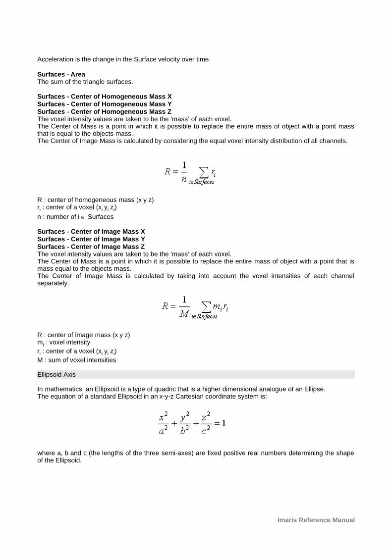
Imaris Reference Manual
Acceleration is the change in the Surface velocity over time.
Surfaces - AreaThe sum of the triangle surfaces.
Surfaces - Center of Homogeneous Mass XSurfaces - Center of Homogeneous Mass YSurfaces - Center of Homogeneous Mass ZThe voxel intensity values are taken to be the ‘mass’ of each voxel.The Center of Mass is a point in which it is possible to replace the entire mass of object with a point massthat is equal to the objects mass.The Center of Image Mass is calculated by considering the equal voxel intensity distribution of all channels.
R : center of homogeneous mass (x y z)ri : center of a voxel (xi yi zi)
n : number of i Î Surfaces
Surfaces - Center of Image Mass X Surfaces - Center of Image Mass YSurfaces - Center of Image Mass ZThe voxel intensity values are taken to be the ‘mass’ of each voxel.The Center of Mass is a point in which it is possible to replace the entire mass of object with a point that ismass equal to the objects mass.The Center of Image Mass is calculated by taking into account the voxel intensities of each channelseparately.
R : center of image mass (x y z)mi : voxel intensity
ri : center of a voxel (xi yi zi)
M : sum of voxel intensities
Ellipsoid Axis
In mathematics, an Ellipsoid is a type of quadric that is a higher dimensional analogue of an Ellipse. The equation of a standard Ellipsoid in an x-y-z Cartesian coordinate system is:
where a, b and c (the lengths of the three semi-axes) are fixed positive real numbers determining the shapeof the Ellipsoid.
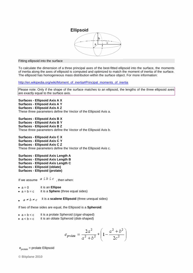
© Bitplane 2010
Fitting ellipsoid into the surface
To calculate the dimension of a three principal axes of the best-fitted ellipsoid into the surface, the momentsof inertia along the axes of ellipsoid is computed and optimized to match the moment of inertia of the surface.The ellipsoid has homogeneous mass distribution within the surface object. For more information:
http://en.wikipedia.org/wiki/Moment_of_inertia#Principal_moments_of_inertia
Please note: Only if the shape of the surface matches to an ellipsoid, the lengths of the three ellipsoid axesare exactly equal to the surface axis.
Surfaces - Ellipsoid Axis A XSurfaces - Ellipsoid Axis A YSurfaces - Ellipsoid Axis A ZThese three parameters define the Vector of the Ellipsoid Axis a.
Surfaces - Ellipsoid Axis B XSurfaces - Ellipsoid Axis B YSurfaces - Ellipsoid Axis B ZThese three parameters define the Vector of the Ellipsoid Axis b.
Surfaces - Ellipsoid Axis C XSurfaces - Ellipsoid Axis C YSurfaces - Ellipsoid Axis C ZThese three parameters define the Vector of the Ellipsoid Axis c.
Surfaces - Ellipsoid Axis Length ASurfaces - Ellipsoid Axis Length BSurfaces - Ellipsoid Axis Length CSurfaces - Ellipsoid (oblate)Surfaces - Ellipsoid (prolate)
If we assume , then when:
· a = 0 it is an Ellipse
· a = b = c it is a Sphere (three equal sides)
·it is a scalene Ellipsoid (three unequal sides)
If two of these sides are equal, the Ellipsoid is a Spheroid:
· a = b < c it is a prolate Spheroid (cigar-shaped)
· a < b = c it is an oblate Spheroid (disk-shaped)
eprolate = prolate Ellipsoid
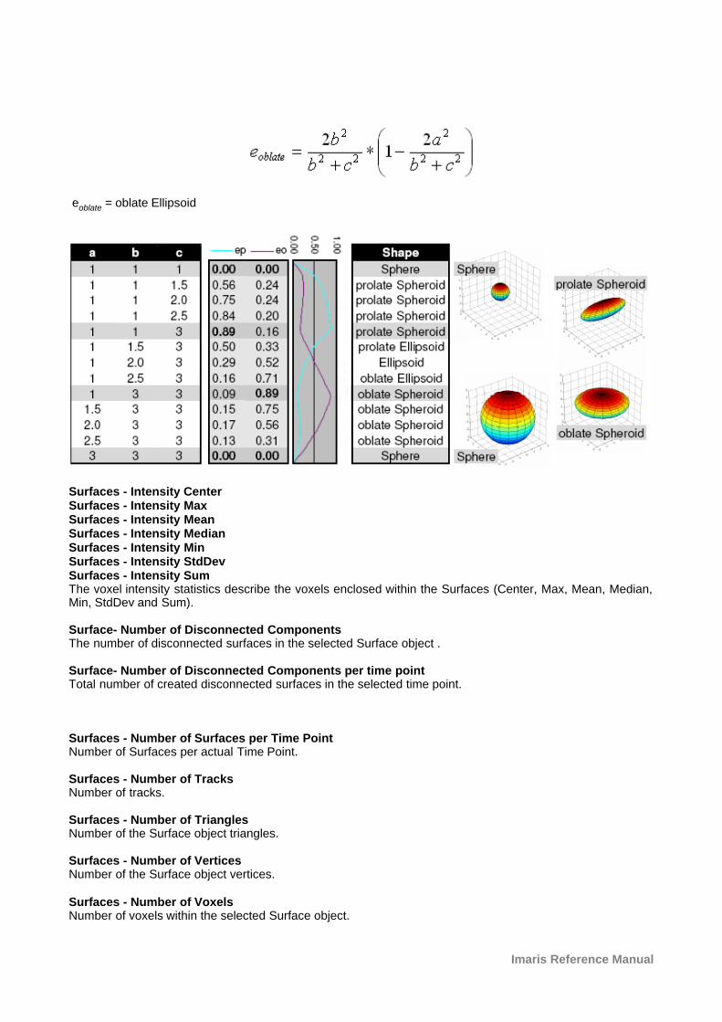
Imaris Reference Manual
eoblate = oblate Ellipsoid
Surfaces - Intensity CenterSurfaces - Intensity MaxSurfaces - Intensity MeanSurfaces - Intensity MedianSurfaces - Intensity MinSurfaces - Intensity StdDevSurfaces - Intensity SumThe voxel intensity statistics describe the voxels enclosed within the Surfaces (Center, Max, Mean, Median,Min, StdDev and Sum).
Surface- Number of Disconnected ComponentsThe number of disconnected surfaces in the selected Surface object .
Surface- Number of Disconnected Components per time pointTotal number of created disconnected surfaces in the selected time point.
Surfaces - Number of Surfaces per Time PointNumber of Surfaces per actual Time Point.
Surfaces - Number of TracksNumber of tracks.
Surfaces - Number of TrianglesNumber of the Surface object triangles.
Surfaces - Number of VerticesNumber of the Surface object vertices.
Surfaces - Number of VoxelsNumber of voxels within the selected Surface object.
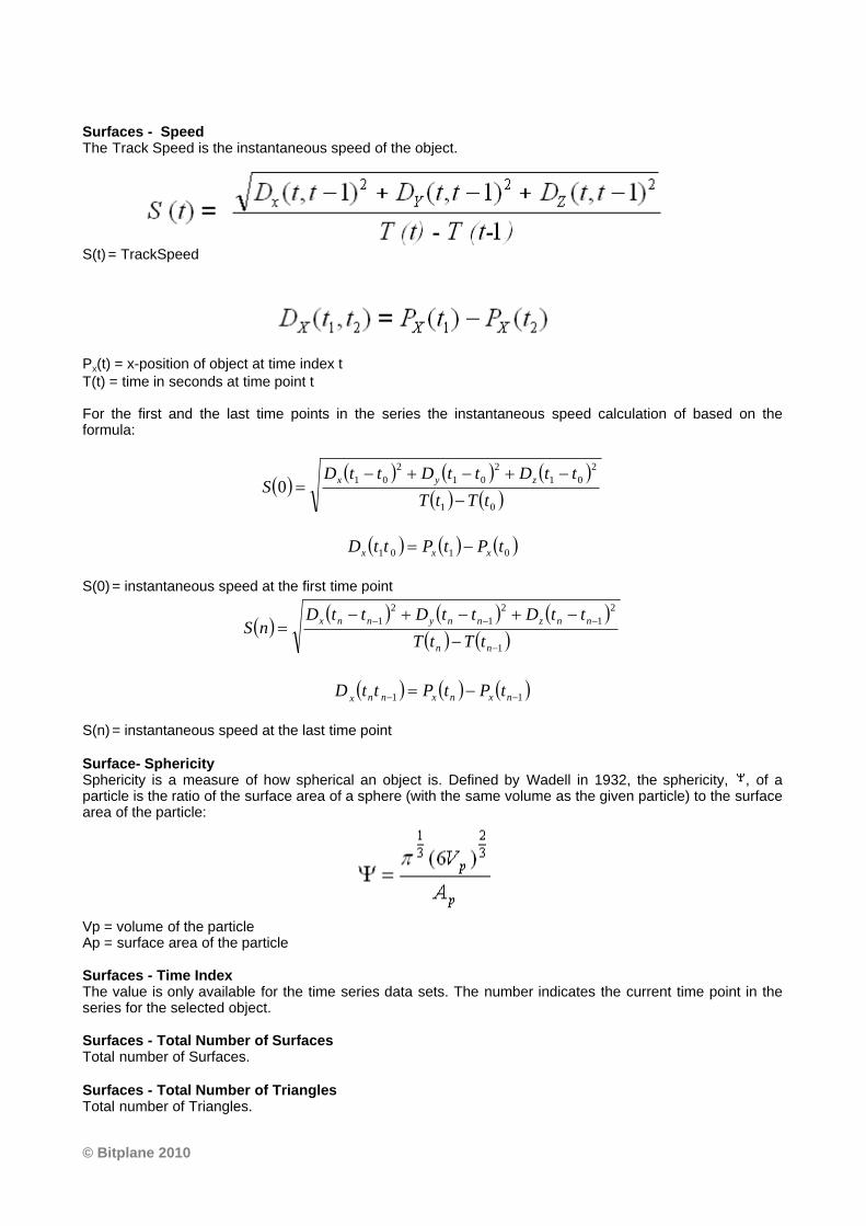
© Bitplane 2010
Surfaces - SpeedThe Track Speed is the instantaneous speed of the object.
S(t) = TrackSpeed
PX(t) = x-position of object at time index tT(t) = time in seconds at time point t
For the first and the last time points in the series the instantaneous speed calculation of based on theformula:
( )( ) ( ) ( )
( ) ( )01
2
01
2
01
2
010
tTtT
ttDttDttDS
zyx
-
-+-+-=
( ) ( ) ( )0101 tPtPttD xxx -=
S(0) = instantaneous speed at the first time point
( )( ) ( ) ( )
( ) ( )1
2
1
2
1
2
1
-
---
-
-+-+-=
nn
nnznnynnx
tTtT
ttDttDttDnS
( ) ( ) ( )11 -- -= nxnxnnxtPtPttD
S(n) = instantaneous speed at the last time point
Surface- SphericitySphericity is a measure of how spherical an object is. Defined by Wadell in 1932, the sphericity, , of aparticle is the ratio of the surface area of a sphere (with the same volume as the given particle) to the surfacearea of the particle:
Vp = volume of the particle Ap = surface area of the particle
Surfaces - Time IndexThe value is only available for the time series data sets. The number indicates the current time point in theseries for the selected object.
Surfaces - Total Number of SurfacesTotal number of Surfaces.
Surfaces - Total Number of TrianglesTotal number of Triangles.
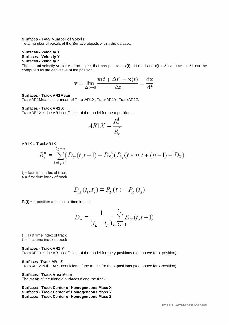
Imaris Reference Manual
Surfaces - Total Number of VoxelsTotal number of voxels of the Surface objects within the dataset.
Surfaces - Velocity XSurfaces - Velocity YSurfaces - Velocity ZThe instant velocity vector v of an object that has positions x(t) at time t and x(t + Dt) at time t + Dt, can becomputed as the derivative of the position:
Surfaces - Track AR1MeanTrackAR1Mean is the mean of TrackAR1X, TrackAR1Y, TrackAR1Z.
Surfaces - Track AR1 XTrackAR1X is the AR1 coefficient of the model for the x-positions.
AR1X = TrackAR1X
tL = last time index of tracktF = first time index of track
PX(t) = x-position of object at time index t
tL = last time index of tracktF = first time index of track
Surfaces - Track AR1 YTrackAR1Y is the AR1 coefficient of the model for the y-positions (see above for x-position).
Surfaces- Track AR1 ZTrackAR1Z is the AR1 coefficient of the model for the z-positions (see above for x-position).
Surfaces - Track Area MeanThe mean of the triangle surfaces along the track.
Surfaces - Track Center of Homogeneous Mass XSurfaces - Track Center of Homogeneous Mass YSurfaces - Track Center of Homogeneous Mass Z
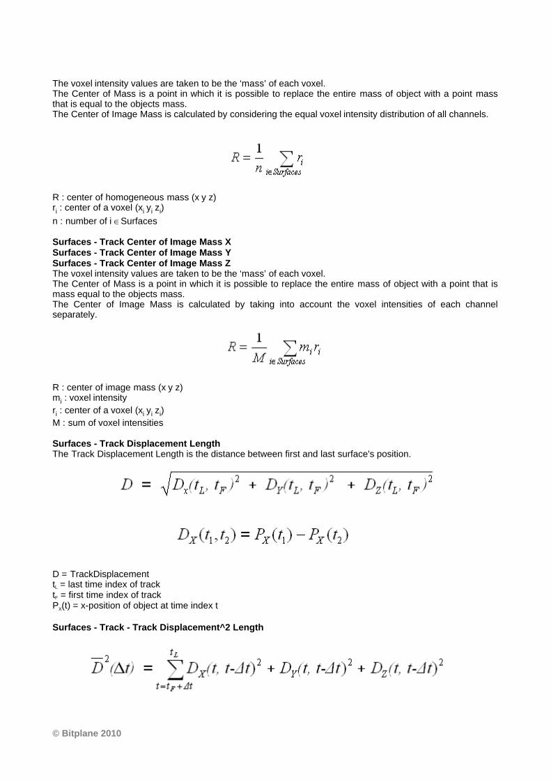
© Bitplane 2010
The voxel intensity values are taken to be the ‘mass’ of each voxel.The Center of Mass is a point in which it is possible to replace the entire mass of object with a point massthat is equal to the objects mass.The Center of Image Mass is calculated by considering the equal voxel intensity distribution of all channels.
R : center of homogeneous mass (x y z)ri : center of a voxel (xi yi zi)
n : number of i ÎSurfaces
Surfaces - Track Center of Image Mass XSurfaces - Track Center of Image Mass YSurfaces - Track Center of Image Mass ZThe voxel intensity values are taken to be the ‘mass’ of each voxel.The Center of Mass is a point in which it is possible to replace the entire mass of object with a point that ismass equal to the objects mass.The Center of Image Mass is calculated by taking into account the voxel intensities of each channelseparately.
R : center of image mass (x y z)mi : voxel intensity
ri : center of a voxel (xi yi zi)
M : sum of voxel intensities
Surfaces - Track Displacement LengthThe Track Displacement Length is the distance between first and last surface's position.
D = TrackDisplacementtL = last time index of tracktF = first time index of trackPX(t) = x-position of object at time index t
Surfaces - Track - Track Displacement^2 Length
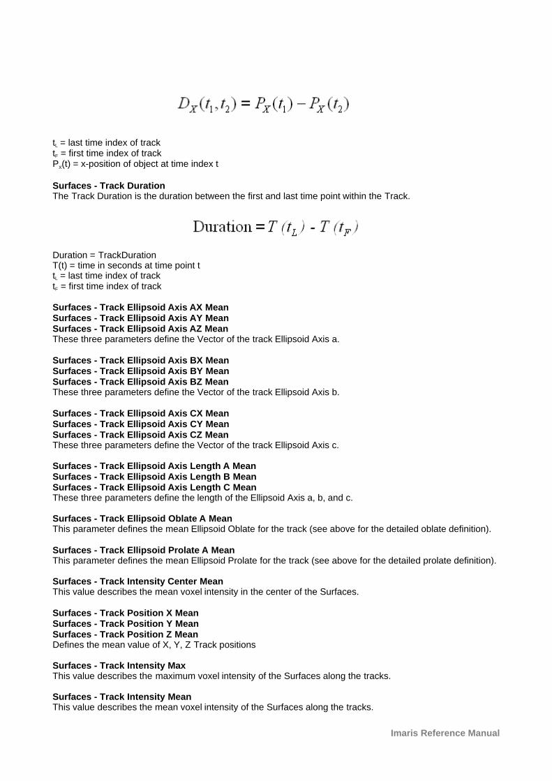
Imaris Reference Manual
tL = last time index of tracktF = first time index of trackPX(t) = x-position of object at time index t
Surfaces - Track DurationThe Track Duration is the duration between the first and last time point within the Track.
Duration = TrackDurationT(t) = time in seconds at time point ttL = last time index of tracktF = first time index of track
Surfaces - Track Ellipsoid Axis AX MeanSurfaces - Track Ellipsoid Axis AY MeanSurfaces - Track Ellipsoid Axis AZ MeanThese three parameters define the Vector of the track Ellipsoid Axis a.
Surfaces - Track Ellipsoid Axis BX MeanSurfaces - Track Ellipsoid Axis BY MeanSurfaces - Track Ellipsoid Axis BZ MeanThese three parameters define the Vector of the track Ellipsoid Axis b.
Surfaces - Track Ellipsoid Axis CX MeanSurfaces - Track Ellipsoid Axis CY MeanSurfaces - Track Ellipsoid Axis CZ MeanThese three parameters define the Vector of the track Ellipsoid Axis c.
Surfaces - Track Ellipsoid Axis Length A MeanSurfaces - Track Ellipsoid Axis Length B MeanSurfaces - Track Ellipsoid Axis Length C MeanThese three parameters define the length of the Ellipsoid Axis a, b, and c.
Surfaces - Track Ellipsoid Oblate A MeanThis parameter defines the mean Ellipsoid Oblate for the track (see above for the detailed oblate definition).
Surfaces - Track Ellipsoid Prolate A MeanThis parameter defines the mean Ellipsoid Prolate for the track (see above for the detailed prolate definition).
Surfaces - Track Intensity Center MeanThis value describes the mean voxel intensity in the center of the Surfaces.
Surfaces - Track Position X Mean Surfaces - Track Position Y Mean Surfaces - Track Position Z Mean Defines the mean value of X, Y, Z Track positions
Surfaces - Track Intensity MaxThis value describes the maximum voxel intensity of the Surfaces along the tracks.
Surfaces - Track Intensity MeanThis value describes the mean voxel intensity of the Surfaces along the tracks.
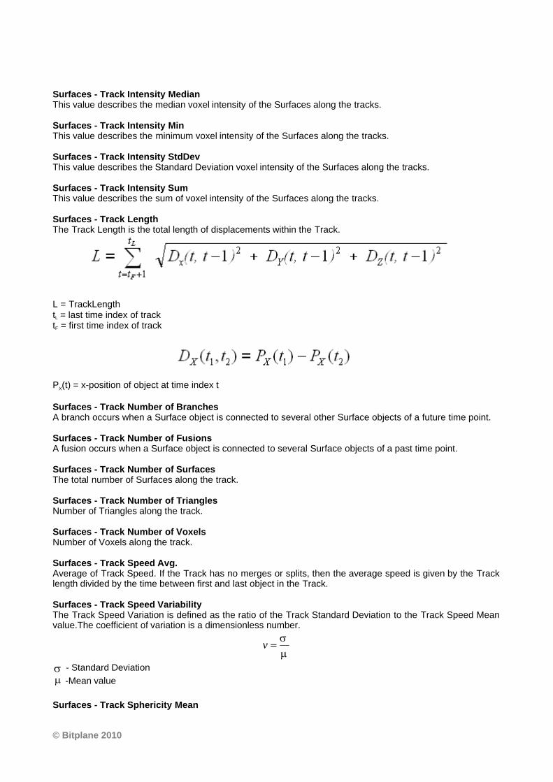
© Bitplane 2010
Surfaces - Track Intensity MedianThis value describes the median voxel intensity of the Surfaces along the tracks.
Surfaces - Track Intensity MinThis value describes the minimum voxel intensity of the Surfaces along the tracks.
Surfaces - Track Intensity StdDevThis value describes the Standard Deviation voxel intensity of the Surfaces along the tracks.
Surfaces - Track Intensity SumThis value describes the sum of voxel intensity of the Surfaces along the tracks. Surfaces - Track LengthThe Track Length is the total length of displacements within the Track.
L = TrackLengthtL = last time index of tracktF = first time index of track
PX(t) = x-position of object at time index t
Surfaces - Track Number of BranchesA branch occurs when a Surface object is connected to several other Surface objects of a future time point.
Surfaces - Track Number of FusionsA fusion occurs when a Surface object is connected to several Surface objects of a past time point.
Surfaces - Track Number of SurfacesThe total number of Surfaces along the track.
Surfaces - Track Number of TrianglesNumber of Triangles along the track.
Surfaces - Track Number of VoxelsNumber of Voxels along the track.
Surfaces - Track Speed Avg. Average of Track Speed. If the Track has no merges or splits, then the average speed is given by the Tracklength divided by the time between first and last object in the Track.
Surfaces - Track Speed VariabilityThe Track Speed Variation is defined as the ratio of the Track Standard Deviation to the Track Speed Meanvalue.The coefficient of variation is a dimensionless number.
m
s=v
s - Standard Deviation
m -Mean value
Surfaces - Track Sphericity Mean
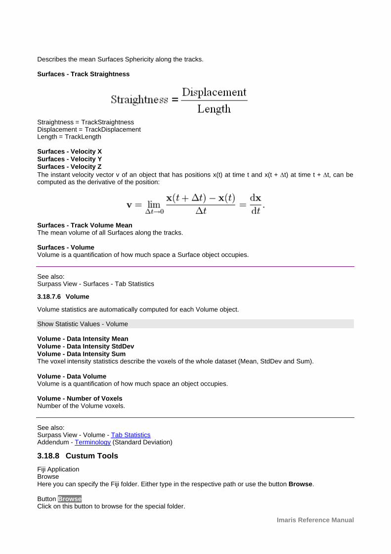
Imaris Reference Manual
Describes the mean Surfaces Sphericity along the tracks.
Surfaces - Track Straightness
Straightness = TrackStraightnessDisplacement = TrackDisplacementLength = TrackLength
Surfaces - Velocity XSurfaces - Velocity YSurfaces - Velocity ZThe instant velocity vector v of an object that has positions x(t) at time t and x(t + Dt) at time t + Dt, can becomputed as the derivative of the position:
Surfaces - Track Volume MeanThe mean volume of all Surfaces along the tracks.
Surfaces - VolumeVolume is a quantification of how much space a Surface object occupies.
See also:Surpass View - Surfaces - Tab Statistics
3.18.7.6 Volume
Volume statistics are automatically computed for each Volume object.
Show Statistic Values - Volume
Volume - Data Intensity MeanVolume - Data Intensity StdDevVolume - Data Intensity SumThe voxel intensity statistics describe the voxels of the whole dataset (Mean, StdDev and Sum).
Volume - Data VolumeVolume is a quantification of how much space an object occupies.
Volume - Number of VoxelsNumber of the Volume voxels.
See also:Surpass View - Volume - Tab StatisticsAddendum - Terminology (Standard Deviation)
3.18.8 Custum Tools
Fiji ApplicationBrowseHere you can specify the Fiji folder. Either type in the respective path or use the button Browse.
Button BrowseClick on this button to browse for the special folder.
© Bitplane 2010
Button OKTo apply the changes click on OK.
Button CancelIf you do not want to save the changes click on Cancel.
3.18.9 Licenses
Here you can adjust the default license settings.
Available Licenses/Licenses Found
Feature LicensesDisplay of all existing Imaris licenses on the system. If a particular license is currently not available (anothercomputer is probably using it), it will be displayed grayed. You can select with which license(s) your Imarisshould start per default. Any change will require a new start of Imaris.
Check/Uncheck AllCheck this box and all available Imaris licenses on the system are selected.
File Reader LicensesDisplay of the actual available file reader licenses on the system.
Check/Uncheck AllCheck this box and all available file reader licenses on the system are selected.
InformationInformation text field how to configure the settings.
Button OKTo apply the changes click on OK.
Button CancelIf you do not want to save the changes click on Cancel.
See also:Menu Help - License...
3.18.10 Update
Here you can adjust the default update settings.
How often should be searched for updates?
DailyWeeklyNeverSelect either daily, weekly, or never.
Button OKTo apply the changes click on OK.
Button CancelIf you do not want to save the changes click on Cancel.
Imaris Reference Manual
3.18.11 Usage Data
Here you can enable the capturing of data usage .
Button OKTo apply the changes click on OK.
Button CancelIf you do not want to save the changes click on Cancel.
3.18.12 3D Cursor
Here you can adjust the default 3D Cursor settings.
3D Cursor
BoxSphereCrossTorusHere you can select the shape of the 3D Cursor.
SizeColorHere you can select the size and color of the 3D Cursor.
Animation
This are the default animation parameters for the function InMotion.
FrequencyAdjust the animation frequency.
Amplitude XAmplitude YAdjust the amplitude in x-, and y-direction.
ShearRotateSelect shear or rotate as animation mode.
ContinuousDiscreteSelect continuous or discrete as animation sequence.
Button OKTo apply the changes click on OK.
Button CancelIf you do not want to save the changes click on Cancel.
See also:InMotion
3.18.13 InPress
Here you can adjust the default InPress settings.
Format
© Bitplane 2010
Title FormatText Format Legend FormatChoose title format, text format or legend format and adjust the following parameter set.
Title, Text or Legend
FontFont SizeColorFormatBoldItalicUnderlinedThe font, font size, color, and format can be selected (from any installed system font).
Button Select...Click on this button to open the color selection window to change the respective color.
Style
Arrow ColorArrow WidthArrow StyleText Box ColorText Box TransparencyText Box StyleYou can adjust the arrow color, width and style (Sphere, Arrow, Magnifier), text box color, transparency andstyle (Unicolor, Black Text, Black Title).
Button Select...Click on this button to open the color selection window to change the respective color.
Button OKTo apply the changes click on OK.
Button CancelIf you do not want to save the changes click on Cancel.
3.18.14 Advanced
Displays a window similar to the parameters window. It shows internal settings and parameters in groups andparameter lists.
Please keep in mind: Changing the advanced parameter settings may endanger your system and lead toerroneous shutdowns!
Button Reset RegistryClick on this button reset registry values to their default settings.
Button OKTo apply the changes click on OK.
Button CancelIf you do not want to save the changes click on Cancel.
Imaris Reference Manual
3.19 File Type Associations...
The file association dialog for the thumbnail creator (window Imaris Icon and Thumbnail Settings) isdisplayed.
File Extensions
Thumbnails will be created and MetaData will be extracted from all checked file types.
Please note: The feature of the thumbnailextractor is not available for the Macintosh users.
.ims Imaris Series, Imaris Classic
.imx Imaris Scene
.ics .idsNikon ICS
.lsmZeiss LSM510
.zviZeiss Axiovision
.leiLeica LCS
.lifLeica LIF
.picBiorad MRC 1024/600
.rbinf TILLvisION
.stkMetaMorph STK
.r3d .dvDelta Vision
.oib .oifOlympus OIB/OIF
.iplScanalytics IPLab
.omeOpen Microscopy Environment XML
.inf .infoLeica Series
.tif .tiffZeiss LSM 410, Zeiss LSM 310, Leica TCS-NT, Leica Series, Leica LCS, Olympus FluoView, Olympus cellR,PerkinElmer, TIFF series
More

© Bitplane 2010
Separated by spaces: e.g. ".ims .ics .lsm .zvi".
2D/3D Indicator
The generated thumbnails are created with or without a 2D/3D indicator.
ShowCheck this box to show the indicator at the left upper corner of the thumbnail. There are four different iconsto indicate the image type:
· 2D Image (colored square). · 2D Time Image (pink square and bars).· 3D Image (green cube).· 3D Time Image (blue cube and bars).
4 Menu View
Please refer to chapter:
Slice Ctrl + 1 Slice ViewSection Ctrl + 2 Section ViewGallery Ctrl + 3 Gallery ViewEasy 3D Ctrl + 4 Easy 3D ViewSurpass Ctrl + 5 Surpass ViewAnimation Ctrl + 6 AnimationInMotion Ctrl + 7 InMotionColoc Ctrl + 8 Coloc
Fit Ctrl + B100% Ctrl + AFull Screen F11Navi Ctrl + N
Origin Bottom LeftOrigin Top LeftOrigin Bottom RightOrigin Top Right
Status Bar Toolbars - Status Bar
Refresh Ctrl + F
See also:Addendum - Mouse & Keyboard Mac
4.1 Fit
Fits the entire scene into the view.
In the Status Bar you find the respective button Fit.
See also:Toolbars - Status Bar
Imaris Reference Manual
4.2 100%
Select 100% to rotate the image to the original position, center the image in the middle and set the zoomfactor to one pixel per voxel.In the Status Bar you find the respective button 100%.
See also:Toolbars - Status Bar
4.3 Full Screen
Displays the viewing area to full size of the monitor. To return to the standard window, click on the button FullScreen in the lower left corner.
In the Status Bar you find the respective button Full Screen.
See also:Toolbars - Status Bar
4.4 Navi
The Navigation window displays an overview of the data set in the upper right corner of the viewing area. Ifyou move the data set the overview updates in real-time. You can activate the Navigation window individuallyfor each Imaris view.
In the Status Bar you find the respective button Navi.
Change Position
· In the pointer mode Select you can click & drag the Navigation window to any desired corner.· Double-click onto the Navigation window in order to switch off the automatic "snap-to-corner-mode". You
can drag it to any desired location. Re-double-click onto the Navigation window to switch the automatic"snap-to-corner-mode" on again.
· Right-click into the Navigation window in order to pan to the clicked position (moves the small yellowwindow).
In the Section view the position of the Navigation window is fixed (lower right corner) and can not be moved.
See also:Section ViewToolbars - Status BarSurpass View - Overview - Camera Toolbar (Pointer Select)
4.5 Origin
The location of the coordinate system origin can be set to any corner of all the views. It can be set to: BottomLeft (default), Top Left, Bottom Right, or Top Right.A selection is stored and used each time you start Imaris.
4.6 Refresh
Refresh the screen.
© Bitplane 2010
5 Menu Image Processing
The Image Processing menu provides a range of functions to change the image data. Frequently usedfunctions are Baseline Subtraction, and Threshold Cutoff from the Image Thresholding submenu or theGaussian Filter from the Image Smoothing submenu.
Button ApplyIf a time series is loaded, clicking Apply applies the image processing function to the current time pointdisplayed on the screen.
Button OKClicking OK applies the image processing function to all time points.
Flip ...Rotate...Channel Shift...Swap Time and ZSwap Time and Channels
SmoothingGaussian Filter...Median Filter...
ThresholdingBaseline Subtraction...Threshold Cutoff...Background Subtraction...Connective Baseline...
Contrast RangeLinear Stretch...Gamma Correction...Invert...Normalize Layers...Histogram Equalization
AutoDeblur...
5.1 Flip...
The channels can be flipped together or separately.
On the left hand side of the window Flip Channel(s) the actual channel(s) are displayed. Select the channelsto be flipped by marking the check-box on the left.
All Channel(s)
Direction X, Y, ZCheck the requested Direction box.
Button ApplyButton OKButton CancelClick the Apply button. The effect of the change can be seen in the image. If necessary, change thedirection. When the results are satisfactory, click the OK button. The data set is modified. Click Cancel toreturn to the original image.
Button Add to Batch Add to Batch button places the command into Batch coordinator.
Imaris Reference Manual
5.2 Rotate...
Rotate direction applies to all channels together. Single channel application is not possible.
All Channel(s)
Axis X, Y, ZEnter the requested axis.
OrientationCounter Clockwise, ClockwiseSelect the respective orientation.
Button ApplyButton OKButton CancelClick the Apply button. The effect result can be seen in the image. If necessary, change the direction. Whenthe results are satisfactory, click the OK button. The data set is modified. Click Cancel to return to theoriginal image.
Button Add to Batch Add to Batch button places the command into Batch coordinator.
5.3 Free Rotate
The Free Rotation function rotates an image by any degree and offers additional image resizing options. Thecamera location determines the rotation angles and directions. The center of the image is the center point ofthe rotation. The operation is preformed for every time point and channel. Please note selecting just one channel for free rotation will create two data sets.
X, Y, Z
These fields display the current x-, y-, and z-values. To alter the image position you can write the values directly into the fields or you can as well adjust the imageposition in the Surpass View.
Angle
This field displays the current value of the angle of rotation.
Coordinate resize factor
The image and voxel values define the size of the new data set after free rotation. These values are used to build a map of all the co-ordinates that will be used to display the newly rotatedimage.
Free rotation can be an expensive memory operation. Adjusting the image dimensions can reduce the size ofthe data set, decreasing the time needed to read the file and speeding up calculation. This can be particularlyimportant when reading large data sets.
Voxel
Changing the x, y, and z values creates a new image with different voxel spacing.These values determine the resampling points. Resampling reduces or increases the voxel density in a dataset.Reducing the resampling points deteriorates the image but speed up any operations on the data.
© Bitplane 2010
X, Y, ZIn the Voxel X, Y and Z fields, enter the factor by which to multiply the current resampling interval.For decimation (fewer samples), enter a factor greater than 1 to increase the sampling interval by this factor.For interpolation (more samples), enter a factor less than 1 to decrease the sampling interval by this factor.
Image
If the border of the new image needs to be adjusted, change the x, y, and z values and create a new imagewith the different image size. This option helps you to crop (minimize the size) the dataset without loosingsignificant data.
X, Y, ZThe parameters X, Y and Z allow you to specify the size of a rotated image by defining the range of anoriginal image. In the Image X, Y and Z fields, enter the crop factor of the lower and upper image range. The values of X, Y and Z should be in the range between 0 and 1.
Padding Intensity
When you create a new image with free rotation some of the new voxel surroundings are included with thedataset. The padding voxels define an area between the previous outside boundary of the original image andnewly rotated image content.This padding intensity field lets you edit the newly created pad voxel intensity.
Linear interpolation
After rotation and data size adjustment, a new image with different voxel spacing is created and the newvoxel coordinates need to be calculated.The difference between the voxel spacing on the new and old image means that an interpolation scheme isrequired as the new image's voxels are unlikely to coincide with those in the old image.The Linear interpolation box allows you to select the interpolation method.If the box is selected for new voxel coordinates then the tri-linear interpolation method is used (allsurrounding values are used for calculations).If the box is not selected the voxel spacing will be calculated based on the nearest neighbor interpolationDepending on the dataset and parameter values the interpolation algorithm could involve some rather timeintensive internal calculations. When speed is favored, please consider selecting the less-time costlyinterpolation method (nearest-neighbor).
5.4 Channel Shift...
The Channel Shift function allows to move channels relative to one another.
On the left hand side of the window Channel Shift the actual channel(s) are displayed. Select the channelsthat should be moved relative to the remaining channels.
Pixel Shift for All Selected Channel(s)
X, Y, ZThe translation is specified in terms of integer numbers of voxels to move along each of the x-, y-, andz-directions.
Button Add to Batch Add to Batch button places the command into Batch coordinator.
5.5 Swap Time and Z
Exchange the t-axis and the z-axis and re-format the image in such a way that the time dimension is mappedonto the z-axis and the z-dimension is mapped onto the t-axis. The section viewer now shows x-t-, and
Imaris Reference Manual
y-t-views.
Start Function
· Select in the menu Image Processing - Swap Time and Z.
The z-, and t-axes are exchanged. This allows you to play the images over z and t.
Play the Series
· Click on Start (arrow to the right) in the Time Bar to play the series of images along the z-axis.
The Time Bar is visible in all display modes (Slice, Section, Gallery 3D Preview, and Surpass). It allows youto view a particular Time Point or to automatically play 4D images. The views change when selecting a newTime Point.
Example:Your data set has four Time Points, each Time Point has one Slice in z-dimension. Then you swap time andz. The result is a new data set with one Time Point and four Slices in z-dimension.
Button Add to Batch Add to Batch button places the command into Batch coordinator.
See also:Toolbars - Time Bar
5.6 Swap Time and Channels
Exchange the t-axis and the channels and re-format the image.
Start Function
· Select in the menu Image Processing - Swap Time and Channels.
The t-axes and the channels are exchanged.
Example:Your data set has four Time Points, each Time Point has one channel. Then you swap time and channel.The result is a new data set with one Time Point and four channels.
Button Add to Batch Add to Batch button places the command into Batch coordinator.
See also:Menu Edit - Image Properties - Channel 1 ... nMenu Edit - Show Display Adjustment
5.7 Extract Channel
The Extract Channels compare the color content of an image to reference color information. This functionextracts and displays color data from the image referent point and use it as a representative color, for a newcolor channel creation. The new channel is generated based on the difference in the reference color pointand the whole image color values. The difference relates how closely the color information in the region matches the information represented bythe color reference point, assigning the higher intensity for smaller difference.The result of the ExtractChannel is a separate channel, which can be processed and viewed as any originally acquired channel inImaris and used for easier segmentation of similarly colored multi-channel data sets.
- Click on the Slice icon in the Main toolbar.
© Bitplane 2010
- Change pointer mode from Navigate to Select.- Select the referent color and click on it. - Clink on the Get value from the last measurement point Button displays associated RGB values in thenumerical fields.- Specify Color Difference by selecting the color space (either RGB or Perceptual).- Select the Apply button. The effect of the change can be seen on the screen.- When the results are satisfactory, click the OK button. - The new channel is created and it’s a part of the data set. - To restore the initial image click Cancel.
The new extracted channel can be visualized like any other channel in Imaris by selecting the Edit menu andchoosing the option Display Adjustment Window. In the Display Adjustment Window un-check originalchannels, select the newly created channel and adjust its setting.
ChannelsThe channels can be selected by clicking on the check box.
Color of InterestThe Color of Interest option allows the reference color point to be present either as separate value for redgreen and blue or as the intensity value for a selected channel. The reference color point is shown within the color wheel.
RGBRGB triple value is displayed for the color reference point.
IntensityIntensity of the selected channel is displayed for the color reference point. Get value from the last measurement point ButtonClicking this button calculates the RGB or intensity values according to the selected color reference point.
Color differenceThis option defines the color space of a newly created channel.
RGBThe RGB color space is an additive color model in which Red, Green and Blue are combined together toreproduce an array of colors.
PerceptualImplements the color extraction using Lab color space. The Lab color model provides a perceptually uniformcolor space. A perceptually uniform color space indicates that a change in a color value produces a changeof about the same visual importance. Lab color is designed to approximate human vision.For more specific information about Lab color space: http://en.wikipedia.org/wiki/Lab_color_space
5.8 Smoothing
Whether or not images need to be smoothed depends on their quality. Inspect the image to see if anysmoothing is required. For image smoothing several different filters are available:
· Gaussian Filter· Median Filter
5.8.1 Gaussian Filter
User Interface
The Gaussian filter for a data set can have only one value. This value can be applied separately to any onechannel or to all channels. Structures smaller than the filter width will be removed.
· Select the menu Image Processing - Image Smoothing - Gaussian Filter. The Gaussian Filter box is
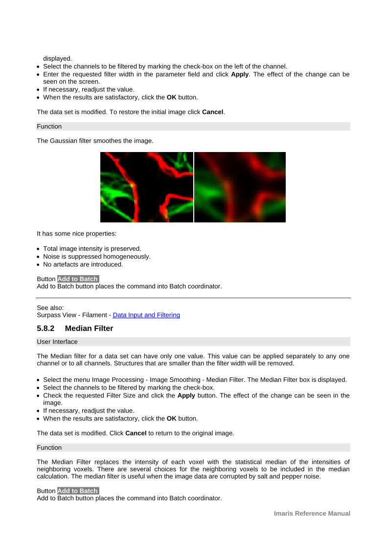
Imaris Reference Manual
displayed.· Select the channels to be filtered by marking the check-box on the left of the channel. · Enter the requested filter width in the parameter field and click Apply. The effect of the change can be
seen on the screen.· If necessary, readjust the value.· When the results are satisfactory, click the OK button.
The data set is modified. To restore the initial image click Cancel.
Function
The Gaussian filter smoothes the image.
It has some nice properties:
· Total image intensity is preserved.· Noise is suppressed homogeneously.· No artefacts are introduced.
Button Add to Batch Add to Batch button places the command into Batch coordinator.
See also:Surpass View - Filament - Data Input and Filtering
5.8.2 Median Filter
User Interface
The Median filter for a data set can have only one value. This value can be applied separately to any onechannel or to all channels. Structures that are smaller than the filter width will be removed.
· Select the menu Image Processing - Image Smoothing - Median Filter. The Median Filter box is displayed.· Select the channels to be filtered by marking the check-box. · Check the requested Filter Size and click the Apply button. The effect of the change can be seen in the
image.· If necessary, readjust the value.· When the results are satisfactory, click the OK button.
The data set is modified. Click Cancel to return to the original image.
Function
The Median Filter replaces the intensity of each voxel with the statistical median of the intensities ofneighboring voxels. There are several choices for the neighboring voxels to be included in the mediancalculation. The median filter is useful when the image data are corrupted by salt and pepper noise.
Button Add to Batch Add to Batch button places the command into Batch coordinator.
© Bitplane 2010
5.9 Thresholding
Whether or not it is necessary to apply a thresholding function to an image depends on its quality. Inspect theimage to see if any action is required.
For image thresholding a number of functions are available. The following paragraphs describe the userinterface to the following filters:
· Threshold Cutoff· Baseline Subtraction· Background Subtraction· Connective Baseline
5.9.1 Threshold Cutoff
Threshold Cutoff compares the intensity of every voxel in the image to the threshold value. If the intensity isgreater than the threshold, it remains unchanged. If a voxels has an intensity less than the threshold value itis assigned a new intensity value. This value is 0 by default. The Threshold Cutoff values for the channelsmay differ.
· Select the menu Image Processing - Image Thresholding - Threshold Cutoff. The Threshold Cutoff box isdisplayed, showing a histogram of the voxels in the data set.
· Select the channels to be cut by marking the check-box to the left of the channel bar. · Highlight a channel.· A colored bar in the histogram shows which channel has been selected.· Enter the requested values for that channel in the Threshold field or drag the bar in the histogram.· Repeat for each channel (if applicable).· Click Apply. The effect of the changes can be seen in the image.· If necessary, readjust the value.· When the results are satisfactory, click the OK button.
Button Add to Batch Add to Batch button places the command into Batch coordinator.
The data set is modified. Click Cancel to return to the original image.
5.9.2 Baseline Subtraction
Baseline Subtraction subtracts the baseline value from the intensity of every voxel in the image. If the resultis positive, this is the new intensity value, if it is negative, the voxels intensity is set to zero. The BaselineSubtraction values for the channels may differ.
· Select the menu Image Processing - Image Thresholding - Baseline Subtraction. The Baseline Subtractionbox is displayed, showing a histogram of the voxels in the data set.
· Select the channels to be cut by marking the check-box to the left of the channel bar. · Highlight a channel.· A colored bar in the histogram shows which channel has been selected.· Enter the requested value for that channel in the Baseline field or drag the bar in the histogram.· Repeat for each channel (if applicable).· Click Apply. The effect of the changes can be seen in the image.· If necessary, readjust the value.· When the results are satisfactory, click the OK button.
Imaris Reference Manual
Button Add to Batch Add to Batch button places the command into Batch coordinator.
The data set is modified. Click Cancel to return to the original image.
5.9.3 Background Subtraction
Background Subtraction applies a Gaussian filter to define the background at each voxel and then performsa Baseline Subtraction of this variable background. The filter width is the only parameter of the backgroundsubtraction method.
· Select the menu Image Processing - Thresholding - Background Subtraction. The Background Subtractionbox is displayed.
· Select the channels by marking the check-box on the left of the channel. · Enter the requested filter width in the parameter field and click Apply. The effect of the change can be
seen on the screen.· If necessary, readjust the value.· When the results are satisfactory, click the OK button.
Button Add to Batch Add to Batch button places the command into Batch coordinator.
5.9.4 Connective Baseline
The Connective Baseline works with two threshold values, a lower and an upper threshold. It applies thesethresholds to divide the image into regions and then processes each region with a Baseline Subtraction usingeither the lower or the upper threshold. The three types of regions the method creates are the following:
· Connected region of voxels where the intensity of every voxel within the region is below the lower threshold(Type A).
· Connected region of voxels where the intensity of every voxel within the region is greater than the lowerthreshold and no voxel within the region has an intensity greater than the upper threshold (Type B).
· Connected region of voxels where the intensity of every voxel within the region is greater than the lowerthreshold and at least one voxel within the region has an intensity greater than the upper threshold (TypeC).
The intensities of voxels from regions of type A are set to zero, as are the intensities of voxels from regionsof type B. Only voxels from regions of type C retain a nonzero intensity, namely the original intensity less thelower threshold value.
Button Add to Batch Add to Batch button places the command into Batch coordinator.
See also:Surpass View - Filament - Data Input
5.10 Contrast Change
For image Contrast Change a number of functions are available. Linear Stretch...Gamma Correction...Invert...Normalize Layer(s)Histogram Equalization
© Bitplane 2010
5.10.1 Linear Stretch...
Linear stretching may be necessary whenever 12 bit data is read in the 16 bit mode. Then the contrast canbe extended to the new limits. Picture data is changed when stretching. Linear stretching results in a picturedisplaying dense data in a wider contrast range.
· Select the menu Image Processing - Contrast Change - Linear Stretch. The Linear Stretch box isdisplayed.
· Select the channels to be stretched by marking the check-box. · Enter the requested values in the parameter fields New Maximum and New Minimum and click the Apply
button. The effect of the change can be seen in the image.· If necessary, readjust the value.· When the results are satisfactory, click the OK button.
The data set is modified. Click Cancel to return to the original image.
Button Add to Batch Add to Batch button places the command into Batch coordinator.
5.10.2 Gamma Correction...
The Gamma correction function lets you improve the image display by intensifying the gray value of a specificrange of voxels. Usually the color contrast values of the voxels stretch linear over a wide range (e.g. 0 - 255).The Gamma correction function lets you set a new gamma value according to which the gamma curve forthe voxels is calculated automatically. Thus the brightness of the voxels can be intensified or weakened incertain areas.
· Select the menu Image Processing - Contrast Change - Gamma Correction. The Gamma Correction boxis displayed with the default Gamma Value set to 1, therefore showing a straight line as a linear voxelrepresentation.
· Select the requested channels by clicking marking the check-box. · Enter the requested value in the Gamma value field or click directly in the gray Gamma Curve area to set
the new gamma value point. The curve and the field value are set accordingly and the effect of the changecan be seen on the channels (channels appear differently).
· Click the Apply button· If necessary, readjust the value.· When the results are satisfactory, click the OK button.
Button Add to Batch Add to Batch button places the command into Batch coordinator.
The data set is modified. Click Cancel to return to the original image
5.10.3 Invert...
The channels can be inverted together or separately.
· Select the menu Image Processing - Contrast Change - Invert. The Invert box is displayed.· Select the channels to be inverted by marking the check-box on the left. The effect of the change can be
seen in the image.· When the results are satisfactory, click the OK button.
The data set is modified.
Button Add to Batch Add to Batch button places the command into Batch coordinator.
Click Cancel to return to the original data set.
Imaris Reference Manual
5.10.4 Normalize Layer(s)
This normalization adjusts brightness and contrast of individual z-slices to a uniform level. It is most useful forcorrecting illumination variations of scans from physical sections, and in some cases it can also reduceattenuation effects from z-stacks. This image processing function first computes the mean and standard deviation values of the intensity for anentire image z-stack. Then it computes mean and Std.dev. for all individual z-slices. Finally, it adjusts theintensities of each z-slice with a linear transformation, to match the overall mean and Std.dev. value.This procedure is applied for all z-slices of the dataset, for all time points and for each channelindependently.Voxels with zero intensity are excluded from this calculation - they are interpreted as background.
· Select the menu Image Processing - Contrast Change - Normalize. · Select the channels to be inverted by marking the check-box on the left and click on the button Apply.· When the results are satisfactory, click the OK button.
The data set is modified.
Button Add to Batch Add to Batch button places the command into Batch coordinator.
Click Cancel to return to the original data set.
5.10.5 Histogram Equalization
Histogram equalization is a method of image processing by contrast adjustment using the image's histogram.The method is useful in images with close contrast values; in particular, this method can lead to better viewsof electron microscopy images.Through this adjustment, the dynamic range and contrast of an image is altered. The resulting imagefeatures the highest possible contrast, uniformly distributed over the whole contrast range. This method increases the global contrast by adjusting the distribution of the intensities on the histogram byspreading out the most frequent values. In histogram equalization, each pixel is assigned a new intensityvalue based on its previous intensity level so that the output image contains a uniform distribution ofintensities. This allows for areas of lower local contrast to gain a higher contrast without affecting the globalcontrast.
Current minimum/maximumThese values define the limits of dataset intensities. Intensities below the Current minimum will be set to the
new minimum and intensities above the Current maximum will be set to the new maximum. New minimum/maximumThese values define the intensity range of the output dataset. By default, they are set to theminimum/maximum achievable intensities of the data set.
To perform histogram equalization on the data set perform the following steps:
· Select the menu Image Processing - Contrast Change - Histogram Equalization. · The Equalize Channel Histogram(s) window is displayed · Select the channels to be processed by marking the check-box · Enter the requested values in the parameter fields Current Minimum/Maximum, New Maximum/Minimum
or accept the automatically optimized Min. and Max. limits.· Click the Apply button.· If necessary, readjust the value.· When the results are satisfactory, click the OK button.
Add to Batch Button Add to Batch button places the command into Batch coordinator.
Click Cancel to return to the original data set.
© Bitplane 2010
5.11 Auto Deblur ...
The AutoDeblur deconvolution software is integrated into Imaris. It requires a separate license. The pathwayto AutoDeblur must be set in the menu Edit - Preferences... - Advanced - Files - AutoDeblurExeFileName.
When opening AutoDeblur, the software will prompt for a destination for the file that is transferred toAutoDeblur and will automatically create an image in the ids/ics format and open it in AutoDeblur.
· Select the menu Image Processing - AutoDeblur ....
An error message appears if the program is not installed or the pathway is not set.
6 Fiji
Imaris Fiji compatible plugins are aimed at performing additional image processing and offering a solution forspecific problems with image analysis. The Imaris Fiji menu allows you to use your current Fiji routines and still continue with your work within theImaris. The Fiji plugins are integrated into Imaris and they can be executed from and within the application,enhancing and extending the functions of Imaris. In the Fiji menu you can find a list of plugins organized into a menu structure. Each plugin collection isdisplayed as a sub menu on this menu. The plugins and macros are stored and run from the Fiji folder.
Image From FijiImage To FijiFileImageProcessAnalyzePluginsOptions...Help..
Please note: This is not an Fiji tutorial. These chapters describe only the usage of Fiji as an integrated part ofImaris.
6.1 Fiji-Imaris
In this chapter you will learn how to integrate Fuji plugins in Imaris by means of the Fiji menu and how toestablish connections between the Fiji and Imaris.
If you already have Fiji installed, skip down directly to the to the Options… section. If you don't have Fiji atall, you have to install it. The latest version can be downloaded from the following locations:
Fiji: http://pacific.mpi-cbg.de/wiki/index.php/Downloads
Depending upon your operating system select the appropriate link. To complete download follow the specific download instructions.
Options...
The first step of integrating the Fiji plugins within Imaris is to specify the folder with the Fiji.exe file. To do thatopen the Fiji menu and choose the last item in the list Options...The Custom Tools window opens. In the field Fiji application either type in the respective path or use thebutton Browse.Specify the Fiji folder and select the .exe file. Click on the OK button.
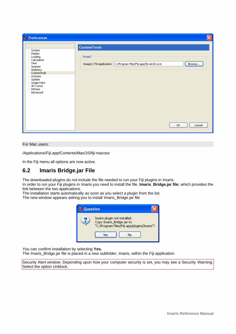
Imaris Reference Manual
For Mac users:
/Applications/Fiji.app/Contents/MacOS/fiji-macosx
In the Fiji menu all options are now active.
6.2 Imaris Bridge.jar File
The downloaded plugins do not include the file needed to run your Fiji plugins in Imaris. In order to run your Fiji plugins in Imaris you need to install the file, Imaris_Bridge.jar file; which provides thelink between the two applications. The installation starts automatically as soon as you select a plugin from the list. The new window appears asking you to install Imaris_Bridge.jar file
You can confirm installation by selecting Yes.The Imaris_Bridge.jar file is placed in a new subfolder, Imaris, within the Fiji application.
Security Alert window: Depending upon how your computer security is set, you may see a Security Warning.Select the option Unblock.
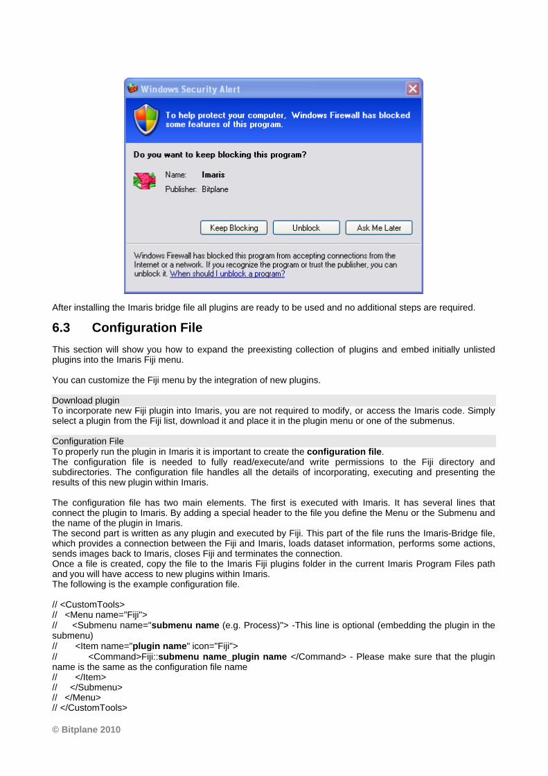
© Bitplane 2010
After installing the Imaris bridge file all plugins are ready to be used and no additional steps are required.
6.3 Configuration File
This section will show you how to expand the preexisting collection of plugins and embed initially unlistedplugins into the Imaris Fiji menu.
You can customize the Fiji menu by the integration of new plugins.
Download plugin To incorporate new Fiji plugin into Imaris, you are not required to modify, or access the Imaris code. Simplyselect a plugin from the Fiji list, download it and place it in the plugin menu or one of the submenus.
Configuration FileTo properly run the plugin in Imaris it is important to create the configuration file. The configuration file is needed to fully read/execute/and write permissions to the Fiji directory andsubdirectories. The configuration file handles all the details of incorporating, executing and presenting theresults of this new plugin within Imaris.
The configuration file has two main elements. The first is executed with Imaris. It has several lines thatconnect the plugin to Imaris. By adding a special header to the file you define the Menu or the Submenu andthe name of the plugin in Imaris. The second part is written as any plugin and executed by Fiji. This part of the file runs the Imaris-Bridge file,which provides a connection between the Fiji and Imaris, loads dataset information, performs some actions,sends images back to Imaris, closes Fiji and terminates the connection.Once a file is created, copy the file to the Imaris Fiji plugins folder in the current Imaris Program Files pathand you will have access to new plugins within Imaris.The following is the example configuration file.
// <CustomTools>// <Menu name="Fiji">// <Submenu name="submenu name (e.g. Process)"> -This line is optional (embedding the plugin in thesubmenu) // <Item name="plugin name" icon="Fiji">// <Command>Fiji::submenu name_plugin name </Command> - Please make sure that the pluginname is the same as the configuration file name// </Item>// </Submenu>// </Menu>// </CustomTools>
Imaris Reference Manual
call("Imaris_Bridge.In", getArgument()); run("plugin name");call("Imaris_Bridge.Out", getArgument()); call("Imaris_Bridge.Terminate", getArgument());
Save the file, and copy it to the special folder:'' C:\Program Files\Bitplane\Imaris version number\imageJPlugins\configurations
Please note: The Imaris version cannot be set differently than the currently running version.
Restart Imaris and the newly inserted plugin will appear in the Fiji menu.
Please note: Imaris Fiji compatible plugins are plugins that provide image data as a result.
6.4 Image From Fiji
Transfer the image to Imaris by selecting the Image From Fiji option.
6.5 Image To Fiji
Transfer the image to Fiji by selecting the Image to Fiji option.
6.6 Initially Installed Plugins
File Open Save
ImageAdjust
Brightness/ contrastColor balanceWindow/Level
ProcessFind EdgesSharpen If you would like to find out more about these plugins, additional information is available in the form the Fijiwebsite.
AnalyzeColor inspector 3D
PluginsLOCI
Plugins are not only used to implement new processing functions, they are also used to support reading andwriting file formats, which are not normally supported by Imaris.
Process
For the detail description it is recommend to visit the Fiji website. There are a lot of examples and tutorials, which could help you to understand the features of these plugins. http://pacific.mpi-cbg.de/wiki/index.php/Fiji's_Menu
RegistrationCorrect 3D DriftLinear Stack Alignment with SIFT
SkeletonAnalyze Skeleton

© Bitplane 2010
http://imagejdocu.tudor.lu/doku.php?id=plugin:analysis:analyzeskeleton:startSkeletonize (2D/3D)
http://imagejdocu.tudor.lu/doku.php?id=plugin:morphology:skeletonize3d:start
6.7 Options...
Custom ToolsHere you can specify the Fiji folder. Either type in the respective path or use the button Browse.
6.8 Fiji Help
Select Help to directly open the Fiji chapter in the Reference Manual.
7 Menu Surpass
Please refer to chapter:
Clipping Plane Surpass View - Clipping PlaneExternal Object Surpass View - External ObjectFilament Surpass View - FilamentFrame Surpass View - FrameGroup Surpass View - GroupLight Source Surpass View - Light SourceMeasurement Point Surpass View - Measurement PointOblique Slicer Surpass View - Oblique SlicerOrtho Slicer Surpass View - Ortho SlicerSpots Surpass View - SpotsSurfaces Surpass View - SurfacesVolume Surpass View - Volume
Export Selected Objects...Delete Selected Objects... Del
Switch View Mode Esc
7.1 Export Selected Objects...
In the Surpass Tree highlight all Items to be exported. To export all Surfaces, Contours, and External objects,select the Export Selected Objects... .
· Select menu Surpass - Export Selected Objects... .
The Save selection as External Objects box is displayed.
· Select the directory and enter the name for the file to be saved and click OK. The object is saved as eitheras an Inventor file with the extension *.iv or as VRML2 file with extension *.vrml. The saved object can beloaded as External objects to another data set.
See also:Surpass View - Overview - Scene File ConceptSurpass View - External Object
7.2 Delete Selected Objects ...
In the Surpass Tree highlight all Items to be deleted. To delete all Surfaces, Spots, Contours, and Externalobjects, select the entire Surpass Scene folder.
Imaris Reference Manual
· Select menu Surpass - Delete Selected Objects.
The Delete selection window with a confirmation question is displayed.
See also:Surpass View - Overview - Surpass Tree - Objects toolbar - Button Delete ...Surpass View - Overview - Scene File Concept
7.3 Switch View Mode
In the Surpass view there are two viewing modes: Select and Navigate.
Select The cursor becomes an arrow. You use the pointer mode Select whenever you want to mark something inthe image, e.g. to set some Measurement Points on the object surface.
NavigateThe cursor becomes two turning arrows. You use the pointer mode Navigate to move, rotate or zoom theimage in the viewing area.
Tip: You can easily switch between the two pointer modes using the ESC-Key. The effect is directly visible onscreen by the altered mouse pointer display.
See also:Surpass View - Overview - Camera Toolbar (Pointer Select or Navigate)
8 Menu Help
Quick Start Tutorials Ctrl + F1Keyboard and Mouse F1Reference ManualProgramming Interface
License... F2Check for Updates now... F3
BitplaneAbout Imaris...
How to find the pdf based help for PC Users:
To open the pdf help file in Imaris first select Start- All Programs – Imaris. The pdf version of the Reference Manual and Quick Start Tutorials are located there.
How to find the pdf based help for Mac Users:
To open the pdf help file in Imaris first locate and select the Imaris application file. By default, the file is in the Application folder and the file name is Imaris 7.2.app. With the right click select the option Show Package Contents. The new window will open. Select the Contents folder and with a double click select the Shared Support folder. The pdf version of the Reference Manual and Quick Start Tutorials are located there.
See also:Addendum - Mouse & Keyboard Mac
© Bitplane 2010
8.1 Quick Start Tutorials
The Quick Start Tutorials provide you with the basic information how-to-use Imaris but may also show yetunrecognized new features of the software to the advanced user.
The tutorials are designed to be followed sequentially, but if you are already familiar with Imaris the basiclessons may be skipped. The tutorials are cross-referenced by hyperlinks highlighted in blue underlined font.The Table of Contents and the Index provide further support for navigation in the tutorials.
Each tutorial is a hands-on seminar, therefore move Imaris to the left hand side of the screen and adjust theonline tutorial on the right hand side of the screen and practice step-by-step.
8.2 Keyboard and Mouse
Click on this menu entry and the Reference Manual opens in the actual browser. The page for the globalMouse & Keyboard functions displays.
Global Mouse & Keyboard Functions
For PC User:
Addendum - Mouse & Keyboard PC
For Mac User:
Addendum - Mouse & Keyboard Mac
8.3 Reference Manual
The Reference Manual provides you with the basic information about Imaris: The menu(s), the differentImaris views and all adjustable parameters in the program.
To find a specific parameter use the "Search function" in the online version of the Reference Manual.
Context Sensitive Help
For PC User:
With a right-click on a toolbar, a tab, or a parameter set the message Show Help... appears. With a left-clickon the massage the Reference Manual opens in the actual browser and displays the corresponding page.
For Mac User:
With a Ctrl + click on a toolbar, a tab, or a parameter set the message Show Help... appears. With a click onthe massage the Reference Manual opens in the actual browser and displays the corresponding page.
8.4 Programming Interface
Select Programming Interface to open the Imaris COM Interface Documentation for ImarisXT.
Imaris Reference Manual
8.5 License...
Two different licensing schemes are available for the software, node-locked and floating. Node-lockedlicenses grant permission to run the licensed software on one computer (node) only. Floating licenses grantpermission to run the licensed software on several computers. One floating license can activate only oneinstance of the program at any given time.
Node-locked licenses are the easiest way to license the software. The installation of node-locked licenses isguided by the Imaris software itself.
Floating licenses require the installation of a separate license server that can run either on a Windows or onan Irix computer. The server installation requires more technical know how.
Install and Upgrade Product Licenses for this Computer
If this computer is connected to the Internet, Imaris can directly download the license informationfrom "www.bitplane.com". Press the "Online" button and follow the instructions.
Button Online...Press this button and follow the instructions.
If this computer has no Internet access you can download the license information via anothercomputer with Internet access. Press the "Offline" button and follow the instructions.
Button Offline...Press this button and follow the instructions.
If this computer should apply license information from a floating license server, or if you would liketo configure a special license file, press this button and follow the instructions.
Button Config...Press this button and follow the instructions.
Button NextPress this button and the window for the Hardware Settings displays (see below). The button Next is onlyavailable after the initial installation of a new Imaris version.
Window: Hardware Settings
The window for the hardware settings is only available after the initial installation of a new Imaris version (seeabove) when you click on the button Next. Imaris will try to figure out the optimal settings for your system anddisplays the values in the fields. You can edit the values. To insert the calculated values again press thebutton Set Default. The hardware settings are adjustable for each user individually. If you want to change thelimits afterwards please go for the Memory Limit to the menu Edit - Preferences... - Calculation and for theTexture Cache Limit to the menu Edit - Preferences... - Display.
Data Cache
Memory LimitThe memory limit defines how much RAM memory Imaris can use before caching on the disk starts. Thevalue must stay below the total amount of installed RAM on the system to work properly. 32-bit systems cannot handle more than 2-3 GB per application.
Display
Texture Cache LimitThe texture cache limit defines how much VideoRAM, RAM Imaris can use for textures. This should be set tothe same value as the amount of VideoRAM on your graphics board.
Open GL Test
© Bitplane 2010
The result of the open GL test displays on the right hand side.· Congratulations, your graphics board is able to display huge data.· Your graphics board is not capable of displaying huge data. Some features will be unavailable.
Automatic Updates
EnableCheck this box and Imaris will look for available updates once a week.
Button Set DefaultClick on this button to insert the calculated values (see above).
Licenses Running on this Computer
NameDisplay of all existing Imaris products and their names.
TypeDisplay of the status of the corresponding license on the computer.
License PathDisplay of the license path. Editable text field.
Button ClearClick on this button to clear the license path.
Host IDDisplay of the host ID. Editable text field.
See also:Menu Edit - Preferences... - CalculationMenu Edit - Preferences... - LicensesMenu Edit - Preferences... - Display
8.6 Check for Updates now ...
If your computer is connected to the Internet, Imaris can directly check, if a software Update is available.
8.7 Bitplane AG
If your computer is connected to the Internet, Imaris can directly open the Bitplane AG homepage (www.bitplane.com).
8.8 About Imaris...
The Imaris start screen displays.
ImarisVersion number and release date.
Copyright 1993-2009 Bitplane AGAll rights reserved
European Patent Registry No. 05009677.7Patent Pending.
Imaris Reference Manual
Using XML parser expat: Copyright1998, 1999, 2000. Thai Open SourceSoftware Center Ltd and Clark Cooper
9 Toolbars
In the standard Imaris view there are three different toolbars available. The Main Toolbar, the Status Bar andthe Time Bar.
See also:Surpass View - Overview - Camera Toolbar
9.1 Main Toolbar
Please refer to chapter:
Open Menu File - OpenSave Menu File- SaveSave as Menu File - Save asSnapshot Menu File - SnapshotInPress Menu File - InPress
The display modes Slice, Section, Gallery and Easy 3D are in one icon group. Click on the arrow to select therespective mode.
Please refer to chapter:
Slice Slice ViewSection Section ViewGallery Gallery ViewEasy 3D Easy 3D View
Surpass Surpass ViewAnimation AnimationInMotion InMotionBatch starts Imaris Batch CoordinatorColoc Coloc
Bitplane AG Menu Help - Bitplane AG
9.2 Status Bar
At the bottom of the screen you find the Status Bar.
Zoom %Imaris lets you enlarge or reduce the view of your data set with the Zoom. You can zoom from 10% to1000%. To go to a predefined zoom level, click the percentage of enlargement or reduction you want. Tospecify a custom level, type a zoom value.
Mouse Clicks to Zoom
With a three-button mouse:
© Bitplane 2010
· Click with the middle mouse button on the image, hold down the middle mouse button, and drag themouse up or down.
· Hold the Shift-key and click with the right mouse button on the image, and drag the mouse up or down.
Tip: In the Surpass view be sure that the mouse is in the pointer mode Navigate. Switch between the twopointer modes Select/Navigate with the ESC-key.
Button 100%Click on this button to rotate the image to the original position, center the image in the middle and set thezoom factor to one pixel per voxel.
Button FitClick on this button to pan the position to best fit in the window and adjust the zoom factor.
Button Full ScreenClick on this button to maximize the viewing area to full size of the monitor. To return to the standard window,click on the button Full Screen in the lower left corner.
Button NaviClick on this button to toggle the display of the Navigation window of the data set in the upper right corner ofthe viewing area. If you move the data set, the overview updates in real-time. In the pointer mode Select youcan click & drag the Navigation window to another position in the viewing area. The Navigation window isplaced to the nearest corner.
Change Position of the Navigation Window
· In the pointer mode Select you can click & drag the Navigation window to any desired corner.· Double-click onto the Navigation window in order to switch off the automatic "snap-to-corner-mode". You
can drag it to any desired location. Re-double-click onto the Navigation window to switch the automatic"snap-to-corner-mode" on again.
· Right-click into the Navigation window in order to pan to the clicked position (moves the small yellowwindow).
In the Section view the position of the Navigation window is fixed (lower right corner) and can not be moved.
See also:Menu View - FitMenu View - 100%Menu View - Full ScreenMenu View - NaviSection ViewSurpass View - Overview - Camera Toolbar (Pointer Navigate/Select)
9.3 Time Bar
If a time series is loaded, a Time Bar displays at the bottom of the main window. It contains a slider showingall Time Points in the series, a Time Settings button, Play and Pause button (arrow to the right), and aRecord button (red dot).
The Time Bar is visible in the display modes Slice, Section, Gallery 3D Preview, and Surpass. It allows you toview a particular Time Point or to automatically play 4D images. The views change when selecting a newTime Point.
Play and Record Time Series
Button Time Settings...Click on this button and you open directly the Time default parameter settings.
Button >Click on this button to play the time series. To pause the continuous display through all the Time Points in the
Imaris Reference Manual
time series re-click on the button.
Button OTo record the time series as movie click on the button Record (red dot). The Save As Movie window isdisplayed (see below).
SliderTo inspect any the Time Point in the time series manually navigate the slider as follows (be sure that thePointer is in the Select mode):
· Drag the slider handle to the left or right.· Moving the slider to the left reduces the time point, moving it to the right increase time point.· Select the slider handle with a left mouse click and then use the Arrow-keys to the left/to the right on the
keyboard.· Select the slider handle with a left mouse click and then press the Home-key or the End-key to display the
first respectively last Time Point.
The respective Time Point number is displayed on the right hand side of the slider in the number field.
Window: Save as Movie
File nameEnter a file name.
Save as typeSelect the desired file type (QuickTimeMovie, TIFF series, or AVI).
Movie Settings
Compression FactorSelect a compression factor between 0 (High Quality) and 100 (Low Quality), the default setting is 5. Use theslider to set the compression factor between 0 and 100. Moving the slider to the left reduces the compressionpoint, moving it to the right increase compression pint. A lower factor results in a lower compression andtherefore a better quality, but also in a larger movie file.
Frame RateDefine how many frames are displayed per second.
Add to ImageAccess databaseCheck the box to add the file to the ImageAccess database.
Play Movie with default Media Player when finishedCheck the box to play the movie with the default media player when finished.
QTVR Settings
The QuickTimeVR Settings are not available.
See also:Menu Edit - Preferences ... - Time (default parameter settings)Surpass View - Overview - Camera Toolbar (Pointer Select)Surpass View - Overview - Camera Toolbar - QuickTimeVR
10 Slice View
How to Open the Slice View?
· Click on the icon in the Main toolbar. If the icon Slice is not displayed click on the arrow in the group:
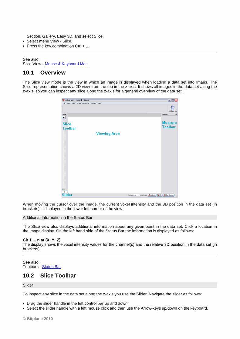
© Bitplane 2010
Section, Gallery, Easy 3D, and select Slice.· Select menu View - Slice.· Press the key combination Ctrl + 1.
See also:Slice View - Mouse & Keyboard Mac
10.1 Overview
The Slice view mode is the view in which an image is displayed when loading a data set into Imaris. TheSlice representation shows a 2D view from the top in the z-axis. It shows all images in the data set along thez-axis, so you can inspect any slice along the z-axis for a general overview of the data set.
When moving the cursor over the image, the current voxel intensity and the 3D position in the data set (inbrackets) is displayed in the lower left corner of the view.
Additional Information in the Status Bar
The Slice view also displays additional information about any given point in the data set. Click a location inthe image display. On the left hand side of the Status Bar the information is displayed as follows:
Ch 1 ... n at (X, Y, Z)The display shows the voxel intensity values for the channel(s) and the relative 3D position in the data set (inbrackets).
See also:Toolbars - Status Bar
10.2 Slice Toolbar
Slider
To inspect any slice in the data set along the z-axis you use the Slider. Navigate the slider as follows:
· Drag the slider handle in the left control bar up and down.· Select the slider handle with a left mouse click and then use the Arrow-keys up/down on the keyboard.
Imaris Reference Manual
· Select the slider handle with a left mouse click and then press the Home-key or the End-key to display thefirst respectively last slice.
· Select the slider handle with a left mouse click and then press the PageDown-key or the PageUp-key todisplay the first respectively last slice.
· Enter the desired slice number in the number field at the bottom of the slider.
Button >Click on the Play/Pause button to see a continuous display through all the slices in the stack. To pausere-click on the button.
Slice Number Field The respective slice number is displayed on the bottom of the slider in the number field.
10.3 Measure Toolbar
Type
LineSet the two Measurement Points with two consecutive clicks. The result is displayed in the status fieldDistance. PolygonAll Measurement Points are consecutively connected by lines and the displayed distance is the sum of thedistances between the points.
GridCheck this box to display a grid in the image.
DistanceThe result of the measurement is displayed in the status field distance.
Button DeleteClick on Delete to clear the status field and start a new measurement.
10.4 Mouse & Keyboard PC
Mouse & Keyboard Functions in the Slice View
Ctrl + 1 Activates the Slice viewLeft-click Set a measurement pointMiddle-click & drag Move up: zoom out
Move down: zoom inShift + right-click & drag Move up: zoom out
Move down: zoom inRight-click & drag Pan image
See also:Addendum - Mouse & Keyboard PC
10.5 Mouse & Keyboard Mac
Mouse & Keyboard Functions in the Slice View
Command + 1 Activates the Slice viewClick Set a measurement point
© Bitplane 2010
With a one-button mouse:
Shift + Ctrl + click & drag Move up: zoom outMove down: zoom in
Ctrl + click & drag Pan image
With a three-button mouse:
To configure a three button mouse on a Mac do the following:· Open the Apple-menu, select System Preferences... . · Click on the button Keyboard & Mouse.· Select the OS X mouse properties.· Change the middle button to "Button 3".
Please note: Combined mouse buttons (e.g. left + middle mouse button) do not work in Imaris.
Middle-click & drag Move up: zoom outMove down: zoom in
Right-click & drag Pan image
See also:Addendum - Mouse & Keyboard Mac
11 Section View
How to Open the Section View?
· Click on the icon in the Main toolbar. If the icon Section is not displayed click on the arrow in the group:Slice, Gallery, Easy 3D, and select Section.
· Select menu View - Section.· Press the key combination Ctrl + 2.
See also:Section View - Mouse & Keyboard Mac
11.1 Overview
The Section view lets you inspect the environment of any given point within the data set by showing the cutthrough the point in the x-, y-, and z-axes or a defined portion of the data set (several slices together).
The illustration below shows the coordinates in the three different display areas of the section view.
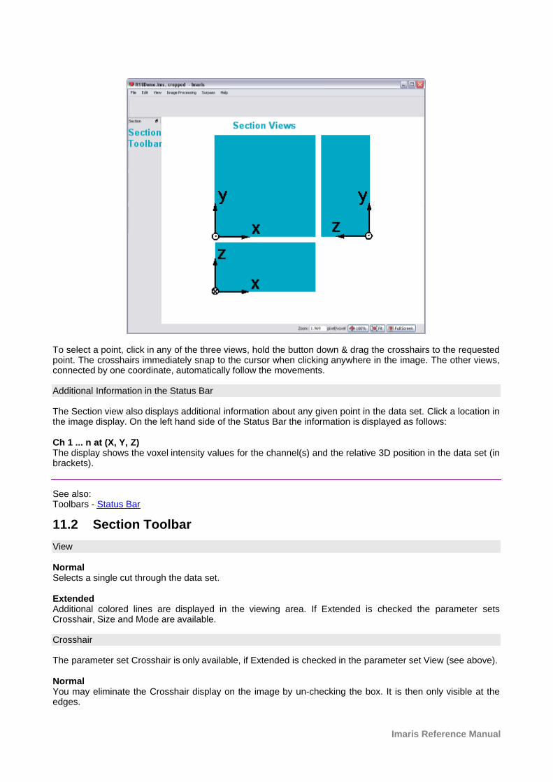
Imaris Reference Manual
To select a point, click in any of the three views, hold the button down & drag the crosshairs to the requestedpoint. The crosshairs immediately snap to the cursor when clicking anywhere in the image. The other views,connected by one coordinate, automatically follow the movements.
Additional Information in the Status Bar
The Section view also displays additional information about any given point in the data set. Click a location inthe image display. On the left hand side of the Status Bar the information is displayed as follows:
Ch 1 ... n at (X, Y, Z)The display shows the voxel intensity values for the channel(s) and the relative 3D position in the data set (inbrackets).
See also:Toolbars - Status Bar
11.2 Section Toolbar
View
NormalSelects a single cut through the data set.
ExtendedAdditional colored lines are displayed in the viewing area. If Extended is checked the parameter setsCrosshair, Size and Mode are available.
Crosshair
The parameter set Crosshair is only available, if Extended is checked in the parameter set View (see above).
NormalYou may eliminate the Crosshair display on the image by un-checking the box. It is then only visible at theedges.
© Bitplane 2010
ExtendedSelect a portion of the data set in the x-, y-, and z-direction to be displayed. In the main screen, separate thetwo crosshairs. The planes between the crosshairs are rendered in the views showing the other axis. Thisallows you to see only certain interior structures without both the top and the bottom.
· The image shows the white crosshair line together with colored focus range lines.· The focus range can be set in any of the three directions as follows: Move the cursor on a colored line. The
cursor changes its form to a straight arrow with a bar.· Drag the line in the respective direction. The range is extended or reduced. Its depth is reflected in the x-,
y-, and z-fields in the Size display. The Size values are indicated in the data set’s dimensions, e.g., in mm. Itcan also be adjusted directly by entering values in the Size fields (see below) or by means of their up anddown arrows.
Un-check the Crosshair – Normal and/or Crosshair – Extended boxes to eliminate the crosshair and/or thefocus range lines display on the image.
Size fields
The parameter set Size is only available, if Extended is checked in the parameter set View (see above).Display of the actual x-, y-, and z-position of the extended Crosshair. The positions can also be adjusteddirectly by entering values in the fields or by means of their up and down arrows.
Mode
The parameter set Mode is only available, if Extended is checked in the parameter set View (see above).Here you may choose the best display mode for the slice portion.
MIPCalculated maximum over all slices in the range.
MeanCalculated mean value over all slices in the range.
BlendCalculated upon the transparency of the slices.
11.3 Mouse & Keyboard PC
Mouse & Keyboard Functions in the Section View
Ctrl + 2 Activates the Section viewLeft-click Set the section centerMiddle-click & drag Move up: zoom out
Move down: zoom inShift + right-click & drag Move up: zoom out
Move down: zoom inRight-click & drag Pan image
See also:Addendum - Mouse & Keyboard PC
11.4 Mouse & Keyboard Mac
Mouse & Keyboard Functions in the Section View
Command + 2 Activates the Section viewClick Set the section center
Imaris Reference Manual
With a one-button mouse:
Shift + Ctrl + click & drag Move up: zoom outMove down: zoom in
Ctrl + click & drag Pan image
With a three-button mouse:
To configure a three button mouse on a Mac do the following:· Open the Apple-menu, select System Preferences... . · Click on the button Keyboard & Mouse.· Select the OS X mouse properties.· Change the middle button to "Button 3".
Please note: Combined mouse buttons (e.g. left + middle mouse button) do not work in Imaris.
Middle-click & drag Move up: zoom outMove down: zoom in
Right-click & drag Pan image
See also:Addendum - Mouse & Keyboard Mac
12 Gallery View
How to Open the Gallery View?
· Click on the icon in the Main toolbar. If the icon Gallery is not displayed click on the arrow in the group:Section, Slice, Easy 3D, and select Gallery.
· Select menu View - Gallery.· Press the key combination Ctrl + 3.
See also:Gallery View - Mouse & Keyboard Mac
12.1 Overview
The Gallery view displays all available slice images of the data set. In the Gallery view you can adapt thedisplay to your needs to gain more information from the slice series. When the Gallery view is selected, allslices are displayed. Click on images to select or deselect them. Selected images are marked with a coloredframe. Holding the Shift-key lets you select a continuous series of images. Hold the Ctrl-key to select variousimages spread over the gallery.
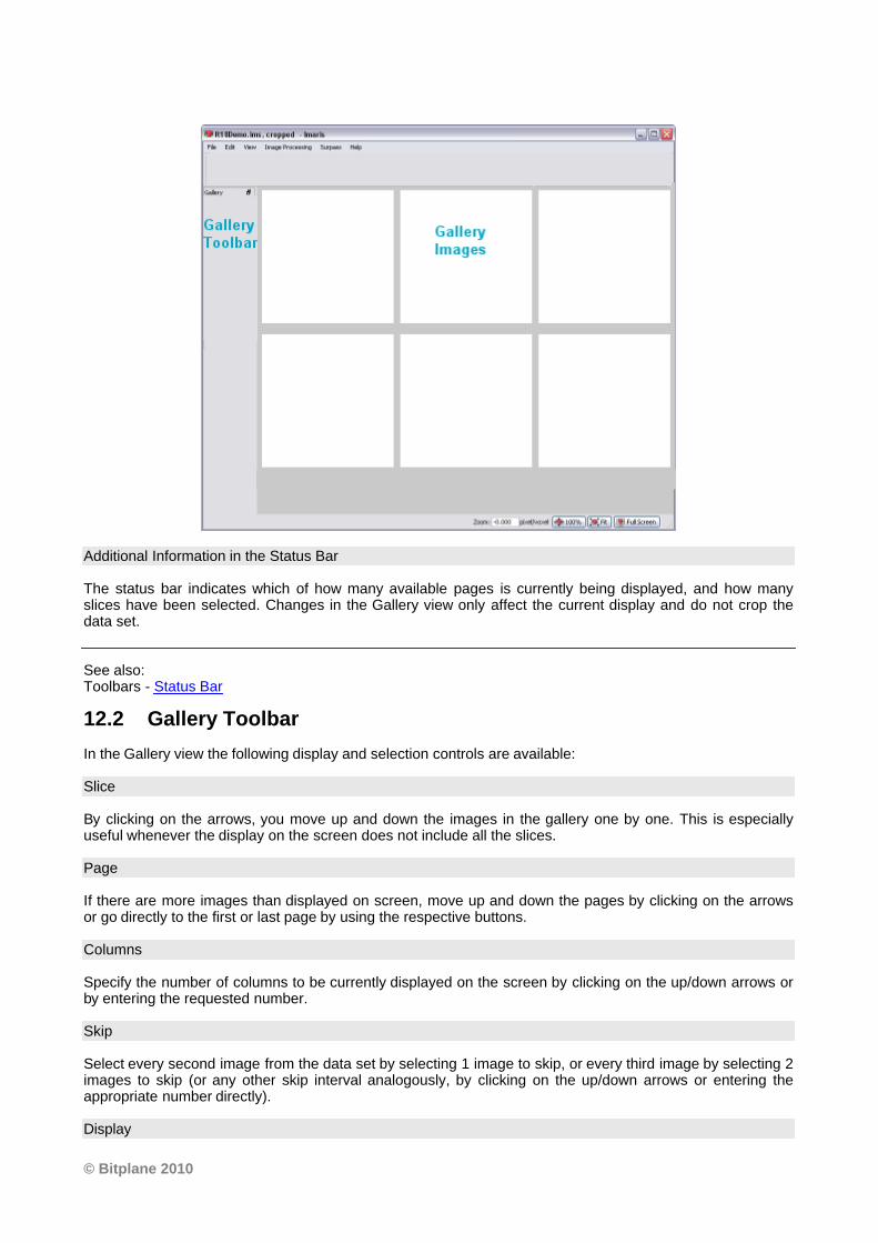
© Bitplane 2010
Additional Information in the Status Bar
The status bar indicates which of how many available pages is currently being displayed, and how manyslices have been selected. Changes in the Gallery view only affect the current display and do not crop thedata set.
See also:Toolbars - Status Bar
12.2 Gallery Toolbar
In the Gallery view the following display and selection controls are available:
Slice
By clicking on the arrows, you move up and down the images in the gallery one by one. This is especiallyuseful whenever the display on the screen does not include all the slices.
Page
If there are more images than displayed on screen, move up and down the pages by clicking on the arrowsor go directly to the first or last page by using the respective buttons.
Columns
Specify the number of columns to be currently displayed on the screen by clicking on the up/down arrows orby entering the requested number.
Skip
Select every second image from the data set by selecting 1 image to skip, or every third image by selecting 2images to skip (or any other skip interval analogously, by clicking on the up/down arrows or entering theappropriate number directly).
Display
Imaris Reference Manual
Button Select...Highlight image(s) and click on the button Select... . Only the selected image(s) is(are) displayed in thegallery. Re-click on the button Select... and all images are displayed in the Gallery.
Slice Number Display
The slice number is displayed beneath each slice.
12.3 Mouse & Keyboard PC
Mouse & Keyboard Functions in the Gallery View
Ctrl + 3 Activates the Gallery viewLeft-click Select sliceCtrl + left-click Add single slice to selectionMiddle-click & drag Move up: zoom out
Move down: zoom inShift + right-click & drag Move up: zoom out
Move down: zoom inRight-click & drag Pan image
See also:Addendum - Mouse & Keyboard PC
12.4 Mouse & Keyboard Mac
Mouse & Keyboard Functions in the Gallery View
Command + 3 Activates the Gallery viewClick Select sliceShift + click Add slices to selectionCommand-click Add single slice to selection
With a one-button mouse:
Shift + Ctrl + click & drag Move up: zoom outMove down: zoom in
Ctrl + click & drag Pan image
With a three-button mouse:
To configure a three button mouse on a Mac do the following:· Open the Apple-menu, select System Preferences... . · Click on the button Keyboard & Mouse.· Select the OS X mouse properties.· Change the middle button to "Button 3".
Please note: Combined mouse buttons (e.g. left + middle mouse button) do not work in Imaris.
Middle-click & drag Move up: zoom outMove down: zoom in
Right-click & drag Pan image
See also:Addendum - Mouse & Keyboard Mac
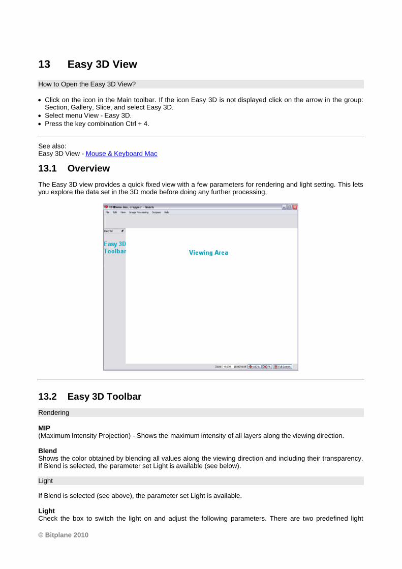
© Bitplane 2010
13 Easy 3D View
How to Open the Easy 3D View?
· Click on the icon in the Main toolbar. If the icon Easy 3D is not displayed click on the arrow in the group:Section, Gallery, Slice, and select Easy 3D.
· Select menu View - Easy 3D.· Press the key combination Ctrl + 4.
See also:Easy 3D View - Mouse & Keyboard Mac
13.1 Overview
The Easy 3D view provides a quick fixed view with a few parameters for rendering and light setting. This letsyou explore the data set in the 3D mode before doing any further processing.
13.2 Easy 3D Toolbar
Rendering
MIP(Maximum Intensity Projection) - Shows the maximum intensity of all layers along the viewing direction.
BlendShows the color obtained by blending all values along the viewing direction and including their transparency.If Blend is selected, the parameter set Light is available (see below).
Light
If Blend is selected (see above), the parameter set Light is available.
LightCheck the box to switch the light on and adjust the following parameters. There are two predefined light
Imaris Reference Manual
setting parameters in Easy 3D Blend to choose from.
Left Light from the left, shadow to the right.
Right Light from the right, shadow to the left.
Button Settings...In Blend mode, with light enabled, click the button Settings.... The Easy 3D Settings dialog box displays (seebelow).
Calculate
AutoThe image is calculated and displayed automatically.
ManualThe image calculation starts after you click on the button Calculate. If you select Manual as calculationmode, the button Calculate is available.
Button CalculateClick on this button to start the calculation for the Easy 3D image view. The button is only available, if youselect Manual as calculation mode.
Window: Easy 3D Settings
Light
Directional Intensity Controls the brightness of structures that are illuminated from the light source.
Ambient Intensity Controls the brightness of structures that are in the shadow. The default (0) means that structures completelyin the shadow are black. The higher the value the brighter the picture and the lower the shadowing contrasts.
Channel Opacity Combination
Allows you to control the opacity of the image.
OpaqueTranslucentCustomSelect Opaque, Transparent, or Custom opacity. It affects only the behavior of interleaving structures of twoor more channels.
13.3 Mouse & Keyboard PC
Mouse & Keyboard Functions in the Easy 3D View
Ctrl + 4 Activates the Easy 3D viewMiddle-click & drag Move up: zoom out
Move down: zoom inShift + right-click & drag Move up: zoom out
Move down: zoom inRight-click & drag Pan image
See also:
© Bitplane 2010
Addendum - Mouse & Keyboard PC
13.4 Mouse & Keyboard Mac
Mouse & Keyboard Functions in the Easy 3D View
Command + 4 Activates the Easy 3D view
With a one-button mouse:
Shift + Ctrl + click & drag Move up: zoom outMove down: zoom in
Ctrl + click & drag Pan image
With a three-button mouse:
To configure a three button mouse on a Mac do the following:· Open the Apple-menu, select System Preferences... . · Click on the button Keyboard & Mouse.· Select the OS X mouse properties.· Change the middle button to "Button 3".
Please note: Combined mouse buttons (e.g. left + middle mouse button) do not work in Imaris.
Middle-click & drag Move up: zoom outMove down: zoom in
Right-click & drag Pan image
See also:Addendum - Mouse & Keyboard Mac
14 Surpass View
The Surpass view provides extended functions for visualization, including:
· A large viewing area with numerous tools for data preparation, presentation and manipulation.· A selection of different types of data display as well as any combination of them.· The possibility of loading additional External objects for comparison.· Grouping functions.
How to Open the Surpass View?
· Click on the icon in the Main toolbar.· Select menu View - Surpass.· Press the key combination Ctrl + 5.
Save and Load Surpass Configuration
The actual Imaris configuration (including Surpass Tree and all existing Items) in the Surpass view is calledSurpass Scene and can be stored in a Scene file with the extension *.imx. The Surpass Scene can be loadedagain to the same data set or to another data set. For details please refer to chapter Surpass View -Overview - Scene File Concept.
See also:Surpass View - Overview - Mouse & Keyboard MacSurpass View - Ortho SliceSurpass View - CellsSurpass View - Clipping PlaneSurpass View - Filament
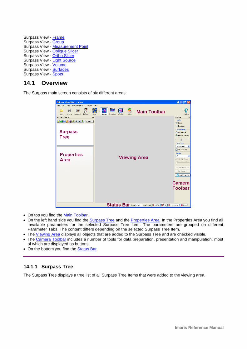
Imaris Reference Manual
Surpass View - FrameSurpass View - GroupSurpass View - Measurement PointSurpass View - Oblique SlicerSurpass View - Ortho SlicerSurpass View - Light SourceSurpass View - VolumeSurpass View - SurfacesSurpass View - Spots
14.1 Overview
The Surpass main screen consists of six different areas:
· On top you find the Main Toolbar.· On the left hand side you find the Surpass Tree and the Properties Area. In the Properties Area you find all
available parameters for the selected Surpass Tree Item. The parameters are grouped on differentParameter Tabs. The content differs depending on the selected Surpass Tree Item.
· The Viewing Area displays all objects that are added to the Surpass Tree and are checked visible.· The Camera Toolbar includes a number of tools for data preparation, presentation and manipulation, most
of which are displayed as buttons.· On the bottom you find the Status Bar.
14.1.1 Surpass Tree
The Surpass Tree displays a tree list of all Surpass Tree Items that were added to the viewing area.
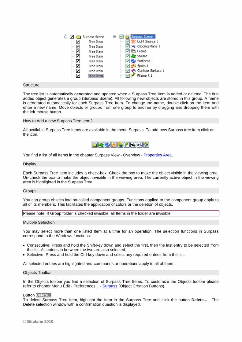
© Bitplane 2010
Structure
The tree list is automatically generated and updated when a Surpass Tree Item is added or deleted. The firstadded object generates a group (Surpass Scene). All following new objects are stored in this group. A nameis generated automatically for each Surpass Tree Item. To change the name, double-click on the item andenter a new name. Move objects or groups from one group to another by dragging and dropping them withthe left mouse button.
How to Add a new Surpass Tree Item?
All available Surpass Tree Items are available in the menu Surpass. To add new Surpass tree item click onthe icon.
You find a list of all Items in the chapter Surpass View - Overview - Properties Area.
Display
Each Surpass Tree Item includes a check-box. Check the box to make the object visible in the viewing area.Un-check the box to make the object invisible in the viewing area. The currently active object in the viewingarea is highlighted in the Surpass Tree.
Groups
You can group objects into so-called component groups. Functions applied to the component group apply toall of its members. This facilitates the application of colors or the deletion of objects.
Please note: If Group folder is checked invisible, all Items in the folder are invisible.
Multiple Selection
You may select more than one listed Item at a time for an operation. The selection functions in Surpasscorrespond to the Windows functions:
· Consecutive: Press and hold the Shift-key down and select the first, then the last entry to be selected fromthe list. All entries in between the two are also selected.
· Selective: Press and hold the Ctrl-key down and select any required entries from the list.
All selected entries are highlighted and commands or operations apply to all of them.
Objects Toolbar
In the Objects toolbar you find a selection of Surpass Tree Items. To customize the Objects toolbar pleaserefer to chapter Menu Edit - Preferences... - Surpass (Object Creation Buttons).
Button Delete...To delete Surpass Tree Item, highlight the Item in the Surpass Tree and click the button Delete... . TheDelete selection window with a confirmation question is displayed.
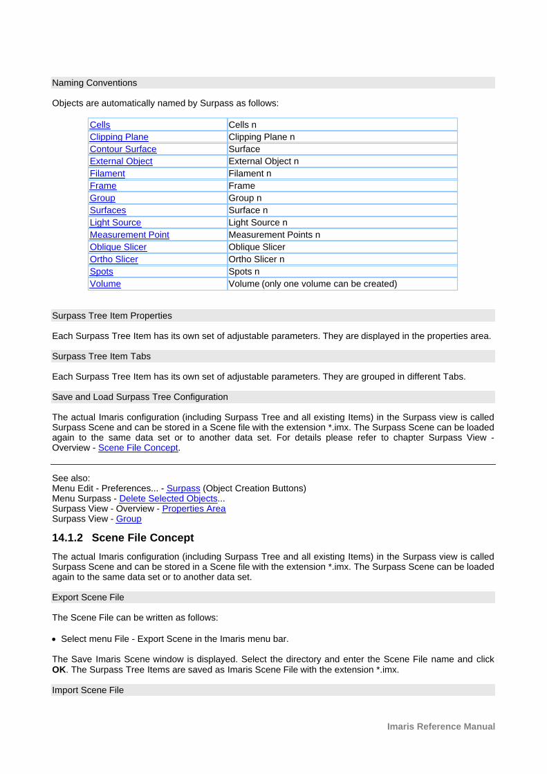
Imaris Reference Manual
Naming Conventions
Objects are automatically named by Surpass as follows:
Cells Cells n
Clipping Plane Clipping Plane n
Contour Surface Surface
External Object External Object n
Filament Filament n
Frame Frame
Group Group n
Surfaces Surface n
Light Source Light Source n
Measurement Point Measurement Points n
Oblique Slicer Oblique Slicer
Ortho Slicer Ortho Slicer n
Spots Spots n
Volume Volume (only one volume can be created)
Surpass Tree Item Properties
Each Surpass Tree Item has its own set of adjustable parameters. They are displayed in the properties area.
Surpass Tree Item Tabs
Each Surpass Tree Item has its own set of adjustable parameters. They are grouped in different Tabs.
Save and Load Surpass Tree Configuration
The actual Imaris configuration (including Surpass Tree and all existing Items) in the Surpass view is calledSurpass Scene and can be stored in a Scene file with the extension *.imx. The Surpass Scene can be loadedagain to the same data set or to another data set. For details please refer to chapter Surpass View -Overview - Scene File Concept.
See also:Menu Edit - Preferences... - Surpass (Object Creation Buttons)Menu Surpass - Delete Selected Objects... Surpass View - Overview - Properties AreaSurpass View - Group
14.1.2 Scene File Concept
The actual Imaris configuration (including Surpass Tree and all existing Items) in the Surpass view is calledSurpass Scene and can be stored in a Scene file with the extension *.imx. The Surpass Scene can be loadedagain to the same data set or to another data set.
Export Scene File
The Scene File can be written as follows:
· Select menu File - Export Scene in the Imaris menu bar.
The Save Imaris Scene window is displayed. Select the directory and enter the Scene File name and clickOK. The Surpass Tree Items are saved as Imaris Scene File with the extension *.imx.
Import Scene File
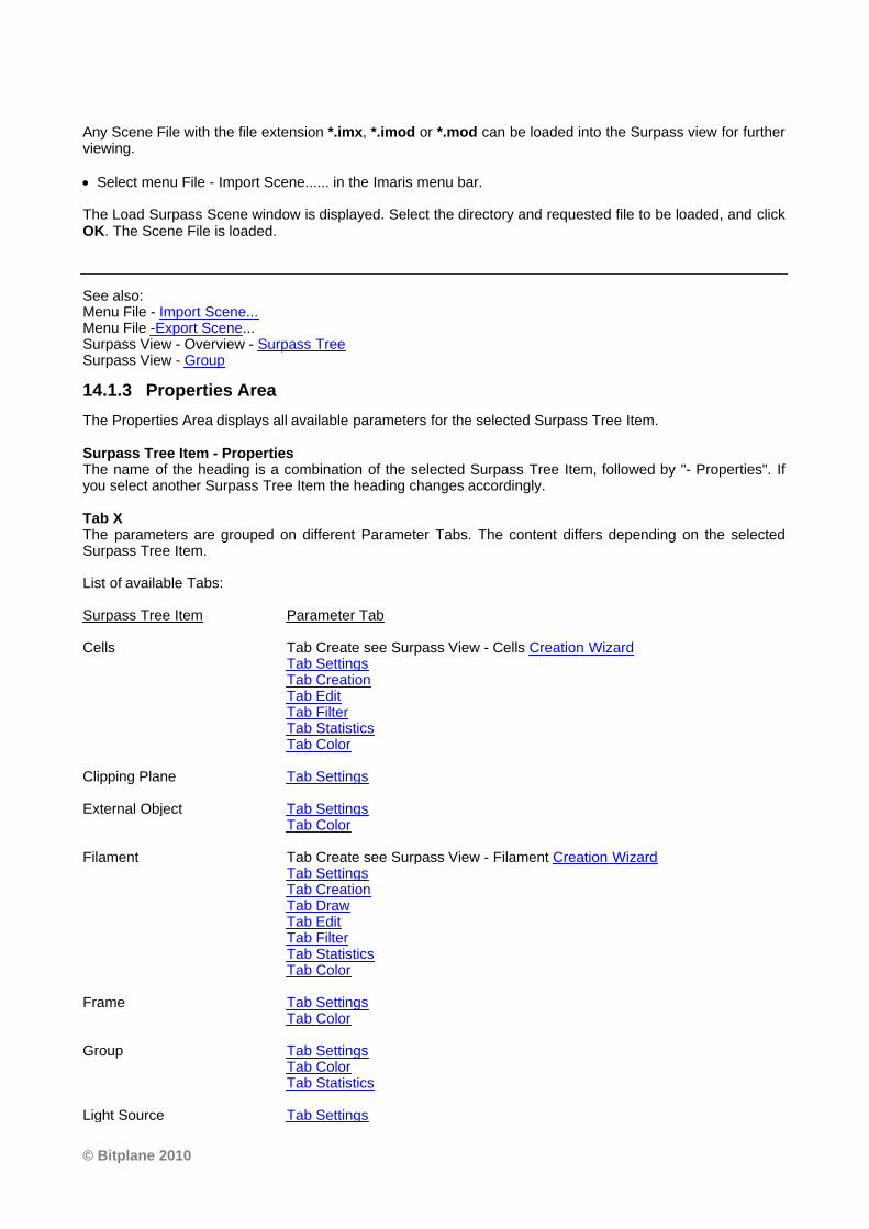
© Bitplane 2010
Any Scene File with the file extension *.imx, *.imod or *.mod can be loaded into the Surpass view for furtherviewing.
· Select menu File - Import Scene...... in the Imaris menu bar.
The Load Surpass Scene window is displayed. Select the directory and requested file to be loaded, and clickOK. The Scene File is loaded.
See also:Menu File - Import Scene...Menu File -Export Scene...Surpass View - Overview - Surpass TreeSurpass View - Group
14.1.3 Properties Area
The Properties Area displays all available parameters for the selected Surpass Tree Item.
Surpass Tree Item - PropertiesThe name of the heading is a combination of the selected Surpass Tree Item, followed by "- Properties". Ifyou select another Surpass Tree Item the heading changes accordingly.
Tab X The parameters are grouped on different Parameter Tabs. The content differs depending on the selectedSurpass Tree Item.
List of available Tabs:
Surpass Tree Item Parameter Tab
Cells Tab Create see Surpass View - Cells Creation WizardTab SettingsTab CreationTab EditTab FilterTab StatisticsTab Color
Clipping Plane Tab Settings
External Object Tab SettingsTab Color
Filament Tab Create see Surpass View - Filament Creation WizardTab SettingsTab CreationTab DrawTab EditTab FilterTab StatisticsTab Color
Frame Tab SettingsTab Color
Group Tab SettingsTab ColorTab Statistics
Light Source Tab Settings
Imaris Reference Manual
Tab Color
Measurement Point Tab SettingsTab EditTab IntensityTab StatisticsTab Color
Ortho Slicer Tab Settings
Oblique Slicer Tab Settings
Spots Tab Create see Surpass View - Spots Creation WizardTab SettingsTab CreationTab EditTab FilterTab StatisticsTab Color
Surfaces Tab Create see Surpass View - Surfaces - Creation WizardTab SettingsTab CreationTab DrawTab EditTab FilterTab StatisticsTab Color
Volume Tab SettingsTab DrawTab Statistics
See also:Surpass View - Overview - Surpass Tree
14.1.4 Creation Wizards
A Creation Wizard is a user interface element where you are led through a sequence of dialogs. In a CreationWizard you are forced to perform a task in a specific sequence.
Examples for Creation Wizards in Imaris are the Cells Creation Wizard, the Filament Creation Wizard, theSpots Creation Wizard, and the Surfaces Creation Wizard. Once you insert an new Item Filament, Spots, orSurfaces you are automatically on the Tab Create in the Properties Area.
See also:Surpass View - Cells - Creation WizardSurpass View - Filament - Creation WizardSurpass View - Spots - Creation WizardSurpass View - Surfaces - Creation Wizard
14.1.5 Viewing Area
Pan
To move the image within the Surpass view (pan the object) choose the mouse pointer mode Navigate. Clickand hold the right mouse button while dragging the mouse. Release right mouse button to place the image.
On a PC or with a three-button mouse or on a Mac:
Right-click & drag Pan image
© Bitplane 2010
On a Mac with a one-button mouse:
Ctrl + click & drag Pan image
Rotate
Rotating an image allows to change the viewing angle on a three-dimensional object.
Choose the mouse pointer mode Navigate. Click with the left mouse button in the image and hold the buttondown while moving the mouse (hold left + drag). The image on screen is rotated towards the direction themouse is dragged. Be sure to hold the left mouse button down during the whole rotation. Stop moving themouse and release the left mouse button to stop the rotation.
On a PC or with a three-button mouse or on a Mac:
Left-click & drag Rotate image
On a Mac with a one-button mouse:
Click & drag Rotate image
How to Keep the Image Continuously Rotated?
Choose the mouse pointer mode Navigate. Click with the left mouse button in the image and hold the buttondown while you move the mouse (hold left + drag). The image on screen is rotated towards the direction themouse is dragged. Release the left mouse button while still dragging the mouse. The result is a continuedrotation (speed of the rotation according to prior mouse motion). To stop the continued rotation re-click in theimage area.
Zoom
In the Surpass view you zoom the image either by using the mouse or by selecting one of the buttons in theStatus Bar at the bottom of the screen.
Using the Mouse
Choose the mouse pointer mode Navigate. To zoom in on the image hold the middle mouse button and dragit towards you. To zoom out from the image hold the middle mouse button and drag it away from you.
On a PC or with a three-button mouse or on a Mac:
Middle-click & drag Move up: zoom outMove down: zoom in
On a Mac with a one-button mouse:
Shift + Ctrl + click & drag Move up: zoom outMove down: zoom in
Using the Buttons in the Status Bar
Zoom %Imaris lets you enlarge or reduce the view of your data set with the Zoom. You can zoom from 10% to1000%. To go to a predefined zoom level, click the percentage of enlargement or reduction you want. Tospecify a custom level, just type a zoom value.
Button 100%Click on this button to rotate the image to the original position, center the image in the middle and set thezoom factor to one pixel per voxel.
Button Fit
Imaris Reference Manual
Click on this button to pan the position to best fit in the window and adjust the zoom factor.
Button Full ScreenClick on this button to maximize the viewing area to full size of the monitor. To return to the standard windowre-click on the button Full Screen in the lower right corner.
See also:Menu ViewToolbars - Status BarSurpass View - Overview - Camera Toolbar (Pointer Navigate)
14.1.6 Camera Toolbar
Pointer
Select The cursor becomes an arrow. You use the pointer mode Select whenever you want to mark something inthe image, e.g. to set some Measurement Points on the object surface.
NavigateThe cursor becomes two turning arrows. You use the pointer mode Navigate to move, rotate or zoom theimage in the viewing area.
Tip: You can easily switch between the two pointer modes using the ESC-key. The effect is directly visible onscreen by the altered mouse pointer display.
Camera Type
Orthogonal Orthogonal display using parallel lines.
Perspective X°Perspective projection is a type of drawing, or rendering, that graphically approximates on a planar(two-dimensional) surface. If you select Perspective the slider (see below) is active.
Slider X°If you select as camera type Perspective X° (see above) the slider is active. Drag the slider to adjust thevertical aperture angle of the camera.
Draw Style
Select the draw style of the object from the drop-down list.
Full Feature Shows all objects as they are.
WireframeDraws Surface objects, Surfaces, Spots, Filaments, and Measurement Points as red colored wireframemodels.
Hidden Lines Draws Surfaces as wireframe models and hides all background lines.
Please note: Set Volume and OrthoSlicer objects invisible before selecting Hidden Lines.
No Texture Draws objects without textures.
Bounding BoxShows only the boxes surrounding the objects.
© Bitplane 2010
Wireframe OverlayLays a red wireframe model over Surface objects, Surfaces, Spots, Filaments, and Measurement Points.
Low ResolutionNot yet implemented.
PointsDraws Surfaces as a point model.
Smooth Lines Check the box to freeze the object in the view area and to prevent movement.
Stereo
OffNo stereo display in the viewing area.
Red/Cyan AnaglyphThis display mode requires colored glasses.
Quad BufferThis display mode requires shutter glasses.
Interleaved RowsThis display mode requires a screen with a lenticular plastic sheet, that overlays the image. The sheet ismolded to have the form of dozens of tiny lenses or prisms per inch.
Interleaved ColumnsThis display mode requires a screen with a lenticular plastic sheet, that overlays the image. The sheet ismolded to have the form of dozens of tiny lenses or prisms per inch.
OffsetDisplay of the offset (0...5).
SliderAdjust the offset to get an optimized 3D effect. Use a small offset if you are far away from the screen, use abig offset, if you are close to the screen. Click on the slider handle and move it to the desired position.
Button Center to SelectionClick on the button Center to Selection to move the selection in the center of the viewing area.
Button Set Center...Use this button to select a new center of rotation. Click on the button Set Center... and then onto theSurpass Scene to define the new center on which the camera zooms in.
Please note: Rotation centers can be set on Surfaces, Contour Surface, Ortho Slicer and External objects
Button Quick Time VRPlease refer to the next chapter: Surpass View - Overview - QuickTimeVR.
14.1.7 QuickTimeVR
You find the Quick Time VR button in the Camera toolbar on the right hand side of the Surpass View.
Button Quick Time VRQuickTimeVR animations show a display rotating around the horizontal or vertical axis, allowing a choice ofthe direction and the angle of rotation. Click on this button to open the Save As Movie window.
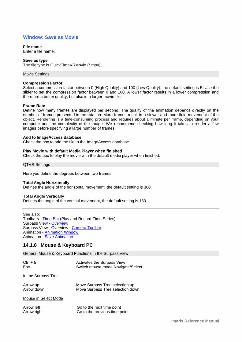
Imaris Reference Manual
Window: Save as Movie
File nameEnter a file name.
Save as typeThe file type is QuickTimeVRMovie (*.mov).
Movie Settings
Compression FactorSelect a compression factor between 0 (High Quality) and 100 (Low Quality), the default setting is 5. Use theslider to set the compression factor between 0 and 100. A lower factor results in a lower compression andtherefore a better quality, but also in a larger movie file.
Frame RateDefine how many frames are displayed per second. The quality of the animation depends directly on thenumber of frames presented in the rotation. More frames result in a slower and more fluid movement of theobject. Rendering is a time-consuming process and requires about 1 minute per frame, depending on yourcomputer and the complexity of the image. We recommend checking how long it takes to render a fewimages before specifying a large number of frames.
Add to ImageAccess databaseCheck the box to add the file to the ImageAccess database.
Play Movie with default Media Player when finishedCheck the box to play the movie with the default media player when finished.
QTVR Settings
Here you define the degrees between two frames.
Total Angle HorizontallyDefines the angle of the horizontal movement, the default setting is 360.
Total Angle Vertically Defines the angle of the vertical movement, the default setting is 180.
See also:Toolbars - Time Bar (Play and Record Time Series)Surpass View - OverviewSurpass View - Overview - Camera ToolbarAnimation - Animation WindowAnimation - Save Animation
14.1.8 Mouse & Keyboard PC
General Mouse & Keyboard Functions in the Surpass View
Ctrl + 5 Activates the Surpass ViewEsc Switch mouse mode Navigate/Select
In the Surpass Tree
Arrow up Move Surpass Tree selection upArrow down Move Surpass Tree selection down
Mouse in Select Mode
Arrow left Go to the next time pointArrow right Go to the previous time point

© Bitplane 2010
Alt Temporary activate Navigate mode (until key is released)Left-click Select objectCtrl + left-click Add object to selection/remove object from selection
Mouse in Navigate Mode
S Set center (on Surfaces, Contour Surface, Ortho Slicer and External objects)Arrow left Go to the next time pointArrow right Go to the previous time pointLeft-click & drag Rotate image (scene)Right-click & drag Pan imageMiddle-click & drag Move up: zoom out
Move down: zoom inShift + right-click & drag Move up: zoom out
Move down: zoom in
See also:Addendum - Mouse & Keyboard PC
14.1.9 Mouse & Keyboard Mac
General Mouse & Keyboard Functions in the Surpass View
Command + 5 Activates the Surpass ViewEsc Switch mouse mode Navigate/Select
In the Surpass Tree
Arrow up Move Surpass Tree selection upArrow down Move Surpass Tree selection down
Mouse in Select Mode
Arrow left Go to the next time pointArrow right Go to the previous time pointClick Select objectCommand-click Add object to selection/remove object from selection
Mouse in Navigate Mode
S Set center (on Surfaces, Contour Surface, Ortho Slices and Externalobjects)
Arrow left Go to the next time pointArrow right Go to the previous time point
With a one-button mouse:
Shift + Ctrl + click & drag Move up: zoom outMove down: zoom in
Ctrl + click & drag Pan imageClick & drag Rotate image
With a three-button mouse:
To configure a three button mouse on a Mac do the following:· Open the Apple-menu, select System Preferences... . · Click on the button Keyboard & Mouse.· Select the OS X mouse properties.· Change the middle button to "Button 3".
Please note: Combined mouse buttons (e.g. left + middle mouse button) do not work in Imaris.
Imaris Reference Manual
Middle-click & drag Move up: zoom outMove down: zoom in
Right-click & drag Pan imageClick & drag Rotate image
See also:Addendum - Mouse & Keyboard Mac
14.2 Cells
ImarisCell is an Imaris module designed specifically to identify, segment, track, measure and analyze Cell,Nucleus and Vesicles in the 2D and 3D time-resolved images. ImarisCell provides simultaneous detection,measurement and analysis of cell objects combined with the interactive identification in the viewing area. ImarisCell calculates and displays detailed statistics values for all the cell’s components and their tracks.Interactive image exploration, simultaneous measurement and analysis of the many features in the imageprovide quick, accurate, quantitative and reproducible results.
How to Add new Cells?
· Select menu Surpass - Cells.
The Surpass Tree list is automatically updated and the first window of the Creation Wizard displays in theCells - Properties.
See also:Surpass View - Cells - Creation Wizard
14.2.1 Creation Wizard
In the first window of the Cells Creation Wizard you find the algorithm settings. Here you have to decide, ifyou want to segment only a Region of Interest (ROI), create Tracks after the Cells objects detection orSkip automatic creation.If you do not want to use the automatic Cell creation wizard select the Skip automatic creation, editmanually button.
Skip automatic creation, edit manually Button Terminates the creation wizard and activates the manual Cells creation.
The Creation Wizard consists of the following steps:AlgorithmRegion of Interest (ROI)DetectionThresholdClassifyTrackingClassify TracksComplete ROI
For further details please refer to Chapters Algorithm, Region of Interest, Detection, Threshold, Classify,Tracking, Classify Tracks, and Complete ROI.
14.2.1.1 Algorithm
Algorithm Settings
Segment only a Region of InterestProcess entire Image Finally
© Bitplane 2010
Track Cells (over time)
If you do not want to use the automatic Cells creation wizard select the Skip automatic creation, editmanually button.
Skip automatic creation, edit manually Button Terminates the creation wizard and activates the Edit options.
Algorithm
Segment only a Region of InterestA Region of Interest (ROI) is a selected sub-region of an image identified for particular processes andanalyzes. Defining and processing ROI allows other parts of an image to be unchanged.Check this box if you want to segment only a Region of Interest. If option Segment only a Region of Interestis selected, in the last step of the Creation Wizard only the region of interest is processed.
Process entire Image finallyThis option appears only, if Segment only a Region of Interest is checked.Check this box and in the last step of the Creation Wizard the entire image is processed with the adjustedparameters (Complete ROI). Un-check this box and only the region of interest is processed.
Track Cells (over Time)Check this box if you want to track the resulting Cells over time, for details please refer to the Tracking Tab.
Cells Wizard Buttons
Button NextPress Next to proceed with the next window of the Creation Wizard.
Button FinishClick on Finish to calculate the desired Cells and display the Cells objects in the viewing area.
Button CancelIf you do not want to create the Cell objects click on Cancel.
14.2.1.2 Region of Interest
Here you define the region of interest (ROI). Parameters such as width, height and location of the ROI areused to directly specify the area to work on.
X, Y, Z, TimeMin, Max, SizeMinimum, maximum and Size of ROI coordinate values can be specified either by entering the value in thevalue fields or by changing the values by clicking on the up-and down arrows on the right hand side of thevalue fields.Alternatively the location and size of the ROI can be adjusted directly in the viewing area. Size of the ROI:1. Click on the ROI preview rectangle arrows (change to the pointer mode Select) 2. Drag the arrows to define new coordinates for X ,Y and Z. Location of the ROI: 1.Click inside the ROI preview rectangle 2. Drag the entire rectangle (with mouse button held) to the chosen image location. The numbers in the value fields are updated automatically.
Memory Usage:Display of the memory usage for the image size within the ROI.
Regions of Interest
To select a particular ROI, left-click on its name in the list and the selected ROI will be highlighted within animage and its properties can be adjusted.
Imaris Reference Manual
Button AddClick on this button and a new region of interest appears in the list. To adjust this ROI you have to select theROI with a left mouse click.
Button DeleteSelect a ROI in the list with a left mouse click and click on this button to delete the ROI.
Total Memory Usage:Display of the memory usage for the image size within the ROI.
Cells Wizard Buttons
Button BackWith Back you return to the previous window of the Creation Wizard.
Button NextPress Next to proceed with the next window of the Creation Wizard.
Button FinishClick on Finish to calculate the desired Cells and display the Cell in the viewing area.
Button CancelIf you do not want to create Cells click on Cancel.
14.2.1.3 Detection
Cell Detection
Source Channel
Select the respective source channel, from which the Cells are to be computed.
Smooth
Check the Smooth option to set up the smoothness of the resulting area. Smoothing applies a Gaussian filterto the data set. Smoothing may require a great deal of memory if the dataset is very large. Un-check the check box or usesmaller ROI if your system does not have enough memory. If the option Smooth is selected then the Filter Width value should be determined. Use either theautomatically given value or type in a new value in the data field.
Filter Width
The value of the Filter Width determines the Gaussian filter width. The value is either automatically calculated from the voxel sizes (oriented at the largest voxel dimension) or itcan be directly entered into the numerical field. The value calculates image coordinates and not voxelsfraction .
Background Subtraction
Background Subtraction applies a Gaussian filter to estimate the background intensity value of each voxel.This variable background is then subtracted from every voxel in the image; Baseline Subtraction isperformed. The width of the Gaussian filter is calculated by subtracting the diameter of the largest sphere that fits intothe Object from the intensity of the original channel.If the option Background Subtraction is selected then the Sphere Diameter should be determined.
Sphere Diameter
The image is processed based on the specified minimum of the object diameter that you have entered. Use
© Bitplane 2010
either the automatically given value or set a new measured value. The value of Sphere Diameter should beslightly larger than the diameter of the largest object expected to be found in the dataset.If the option Background Subtraction is not selected, the Absolute Intensity threshold is performed.
Detect Nuclei
Select this option and the Nucleus objects are included in the automatic creation process.
Source Channel
Select the respective source channel, from which the Nuclei are to be computed.
Smooth
Check the Smooth option to set up the smoothness of the resulting area. Smoothing applies a Gaussian filterto the data set. Smoothing may require a great deal of memory if the dataset is very large. Un-check the check box or usesmaller ROI if your system does not have enough memory. If the option Smooth is selected then the Filter Width value should be determined. Use either theautomatically given value or type in a new value in the data field.
Filter Width
The value of the Filter Width determines the Gaussian filter width. The value is either automatically calculated from the voxel sizes (oriented at the largest voxel dimension) or itcan be directly entered into the numerical field. The value is calculated into image coordinates and not intofraction of voxels.
Background Subtraction
Background Subtraction applies a Gaussian filter to estimate the background intensity value of each voxel.This variable background is then subtracted from every voxel in the image; Baseline Subtraction isperformed. The width of the Gaussian filter is calculated by subtracting the diameter of the largest sphere that fits intothe Object from the intensity of the original channel.If the option Background Subtraction is selected then the Sphere Diameter should be determined.
Sphere Diameter
The image is processed based on the specified minimum of the object diameter that you have entered. Useeither the automatically given value or set a new measured value. The value of Sphere Diameter should beslightly larger than the diameter of the largest object expected to be found in the dataset.If the option Background Subtraction is not selected, the Absolute Intensity threshold is performed.
Detect Vesicles
Select this option to start the automatic creation process for Vesicles.
Source Channel
Select the respective source channel, from which the Vesicles are to be computed.
Estimated Diameter
Objects with size smaller than specified Estimated Diameter are not detected.
Background Subtraction
If checked, the background will be removed prior to Vesicle detection. Technically the backgroundsubtraction is used to smooth the image. The intensity equals the Gaussian filtered channel (Gaussianfiltered by 3/4) minus the intensity of the original channel Gaussian filtered by 8/9 of sphere radius.
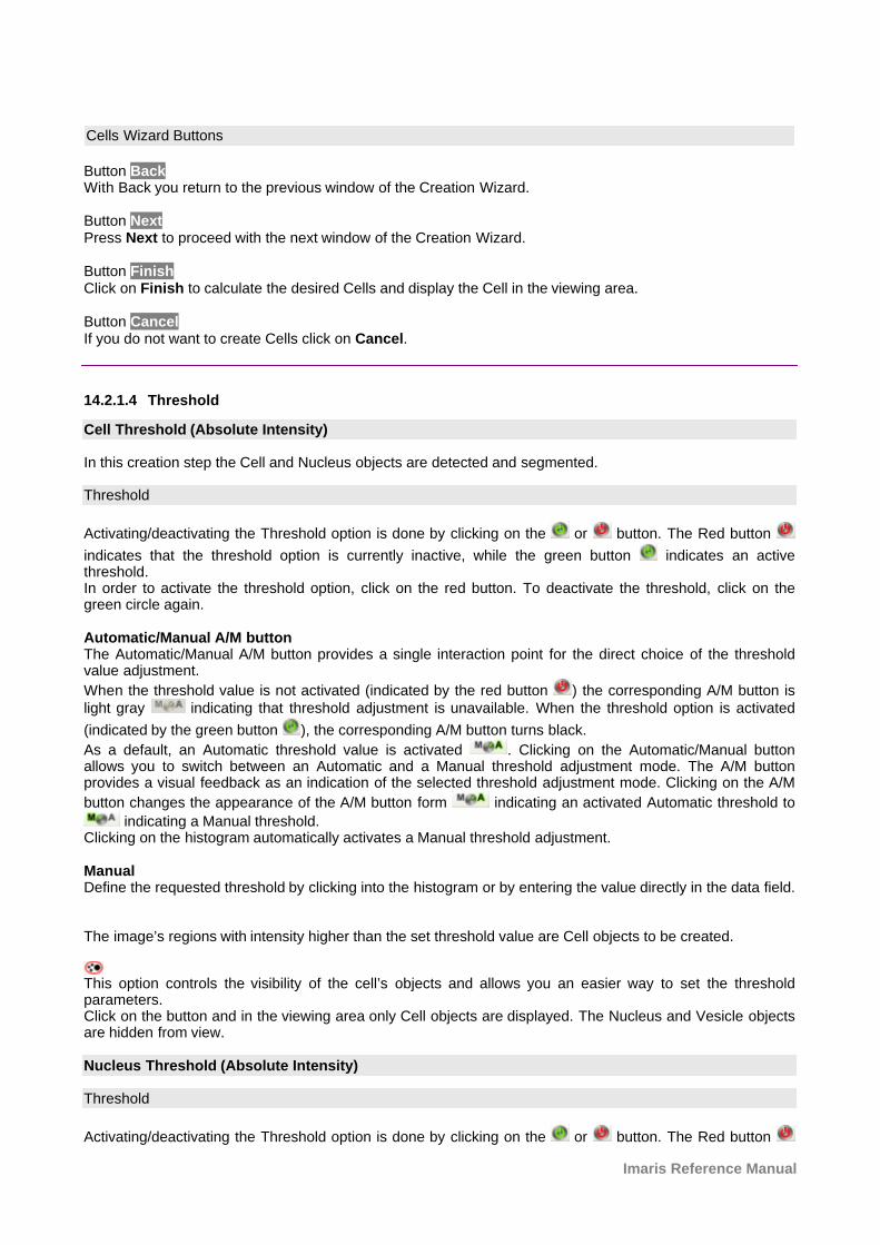
Imaris Reference Manual
Cells Wizard Buttons
Button BackWith Back you return to the previous window of the Creation Wizard.
Button NextPress Next to proceed with the next window of the Creation Wizard.
Button FinishClick on Finish to calculate the desired Cells and display the Cell in the viewing area.
Button CancelIf you do not want to create Cells click on Cancel.
14.2.1.4 Threshold
Cell Threshold (Absolute Intensity)
In this creation step the Cell and Nucleus objects are detected and segmented.
Threshold
Activating/deactivating the Threshold option is done by clicking on the or button. The Red button
indicates that the threshold option is currently inactive, while the green button indicates an activethreshold.In order to activate the threshold option, click on the red button. To deactivate the threshold, click on thegreen circle again.
Automatic/Manual A/M buttonThe Automatic/Manual A/M button provides a single interaction point for the direct choice of the thresholdvalue adjustment.
When the threshold value is not activated (indicated by the red button ) the corresponding A/M button islight gray indicating that threshold adjustment is unavailable. When the threshold option is activated
(indicated by the green button ), the corresponding A/M button turns black.
As a default, an Automatic threshold value is activated . Clicking on the Automatic/Manual buttonallows you to switch between an Automatic and a Manual threshold adjustment mode. The A/M buttonprovides a visual feedback as an indication of the selected threshold adjustment mode. Clicking on the A/M
button changes the appearance of the A/M button form indicating an activated Automatic threshold to
indicating a Manual threshold. Clicking on the histogram automatically activates a Manual threshold adjustment.
ManualDefine the requested threshold by clicking into the histogram or by entering the value directly in the data field.
The image’s regions with intensity higher than the set threshold value are Cell objects to be created.
This option controls the visibility of the cell’s objects and allows you an easier way to set the thresholdparameters. Click on the button and in the viewing area only Cell objects are displayed. The Nucleus and Vesicle objectsare hidden from view.
Nucleus Threshold (Absolute Intensity)
Threshold
Activating/deactivating the Threshold option is done by clicking on the or button. The Red button
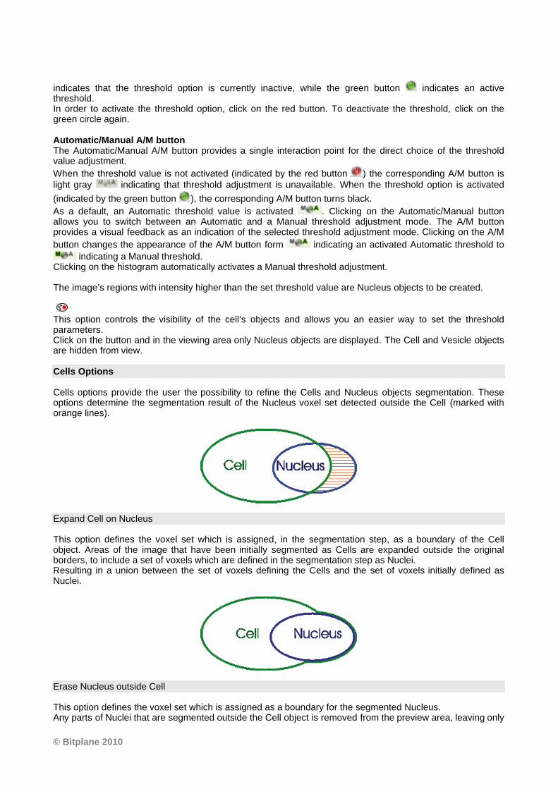
© Bitplane 2010
indicates that the threshold option is currently inactive, while the green button indicates an activethreshold.In order to activate the threshold option, click on the red button. To deactivate the threshold, click on thegreen circle again.
Automatic/Manual A/M buttonThe Automatic/Manual A/M button provides a single interaction point for the direct choice of the thresholdvalue adjustment.
When the threshold value is not activated (indicated by the red button ) the corresponding A/M button islight gray indicating that threshold adjustment is unavailable. When the threshold option is activated
(indicated by the green button ), the corresponding A/M button turns black.
As a default, an Automatic threshold value is activated . Clicking on the Automatic/Manual buttonallows you to switch between an Automatic and a Manual threshold adjustment mode. The A/M buttonprovides a visual feedback as an indication of the selected threshold adjustment mode. Clicking on the A/M
button changes the appearance of the A/M button form indicating an activated Automatic threshold to
indicating a Manual threshold. Clicking on the histogram automatically activates a Manual threshold adjustment.
The image’s regions with intensity higher than the set threshold value are Nucleus objects to be created.
This option controls the visibility of the cell’s objects and allows you an easier way to set the thresholdparameters. Click on the button and in the viewing area only Nucleus objects are displayed. The Cell and Vesicle objectsare hidden from view.
Cells Options
Cells options provide the user the possibility to refine the Cells and Nucleus objects segmentation. Theseoptions determine the segmentation result of the Nucleus voxel set detected outside the Cell (marked withorange lines).
Expand Cell on Nucleus
This option defines the voxel set which is assigned, in the segmentation step, as a boundary of the Cellobject. Areas of the image that have been initially segmented as Cells are expanded outside the originalborders, to include a set of voxels which are defined in the segmentation step as Nuclei. Resulting in a union between the set of voxels defining the Cells and the set of voxels initially defined asNuclei.
Erase Nucleus outside Cell
This option defines the voxel set which is assigned as a boundary for the segmented Nucleus.Any parts of Nuclei that are segmented outside the Cell object is removed from the preview area, leaving only
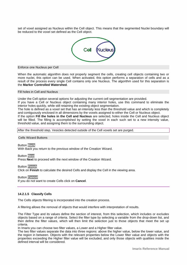
Imaris Reference Manual
set of voxel assigned as Nucleus within the Cell object. This means that the segmented Nuclei boundary willbe reduced to the voxel set defined as the Cell object.
Enforce one Nucleus per Cell
When the automatic algorithm does not properly segment the cells, creating cell objects containing two ormore nuclei, this option can be used. When activated, this option performs a separation of cells and as aresult of the process every single Cell contains only one Nucleus. The algorithm used for this separation isthe Marker Controlled Watershed.
Fill holes in Cell and Nucleus
Under the Cell option several options for adjusting the current cell segmentation are provided. If you have a Cell or Nucleus object containing many interior holes, use this command to eliminate theinterior holes quickly, while still retaining the existing object segmentation. The hole is defined as a voxel set that has an intensity less than the threshold value and which is completelyand contiguously enclosed in all dimensions by the voxels assigned to either the Cell or Nucleus object. If the option Fill the holes in the Cell and Nucleus are selected, holes inside the Cell and Nucleus objectwill be filled. The filling is accomplished by setting the voxel in each such set to a new intensity value,threshold value, and assigning them to the surrounding object.
After the threshold step, Vesicles detected outside of the Cell voxels set are purged.
Cells Wizard Buttons
Button BackWith Back you return to the previous window of the Creation Wizard.
Button NextPress Next to proceed with the next window of the Creation Wizard.
Button FinishClick on Finish to calculate the desired Cells and display the Cell in the viewing area.
Button CancelIf you do not want to create Cells click on Cancel.
14.2.1.5 Classify Cells
The Cells objects filtering is incorporated into the creation process.
A filtering allows the removal of objects that would interfere with interpretation of results.
The Filter Type and its values define the section of interest, from this selection, which includes or excludesobjects based on a range of criteria. Select the filter type by selecting a variable from the drop-down list, andthen define the filter values, which will then limit the selection just to those objects that meet the set upcriteria. In Imaris you can choose two filter values, a Lower and a Higher filter value. The two filter values separate the data into three regions: above the higher value, below the lower value, andthe region in between. Objects with the relevant properties below the Lower filter value and objects with theproperties exceeding the Higher filter value will be excluded, and only those objects with qualities inside thedefined interval will be considered.
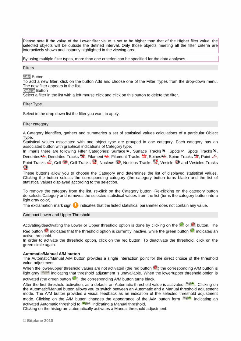
© Bitplane 2010
Please note if the value of the Lower filter value is set to be higher than that of the Higher filter value, theselected objects will be outside the defined interval. Only those objects meeting all the filter criteria areinteractively shown and instantly highlighted in the viewing area.
By using multiple filter types, more than one criterion can be specified for the data analyses.
Filters
Add ButtonTo add a new filter, click on the button Add and choose one of the Filter Types from the drop-down menu.The new filter appears in the list.Delete ButtonSelect a filter in the list with a left mouse click and click on this button to delete the filter.
Filter Type
Select in the drop down list the filter you want to apply.
Filter category
A Category identifies, gathers and summaries a set of statistical values calculations of a particular ObjectType. Statistical values associated with one object type are grouped in one category. Each category has anassociated button with graphical indications of Category type.In Imaris there are following Filter Categories: Surface , Surface Tracks , Spots , Spots Tracks ,
Dendrites , Dendrites Tracks , Filament , Filament Tracks , Spines , Spine Tracks , Point ,
Point Tracks , Cell , Cell Tracks , Nucleus , Nucleus Tracks , Vesicle and Vesicles Tracks
. These buttons allow you to choose the Category and determines the list of displayed statistical values.Clicking the button selects the corresponding category (the category button turns black) and the list ofstatistical values displayed according to the selection.
To remove the category from the list, re-click on the Category button. Re-clicking on the category buttonde-selects Category and removes the selected statistical values from the list (turns the category button into alight gray color).
The exclamation mark sign indicates that the listed statistical parameter does not contain any value.
Compact Lower and Upper Threshold
Activating/deactivating the Lower or Upper threshold option is done by clicking on the or button. The
Red button indicates that the threshold option is currently inactive, while the green button indicates anactive threshold.In order to activate the threshold option, click on the red button. To deactivate the threshold, click on thegreen circle again.
Automatic/Manual A/M buttonThe Automatic/Manual A/M button provides a single interaction point for the direct choice of the thresholdvalue adjustment.
When the lower/upper threshold values are not activated (the red button ) the corresponding A/M button islight gray indicating that threshold adjustment is unavailable. When the lower/upper threshold option is
activated (the green button ), the corresponding A/M button turns black.
After the first threshold activation, as a default, an Automatic threshold value is activated . Clicking onthe Automatic/Manual button allows you to switch between an Automatic and a Manual threshold adjustmentmode. The A/M button provides a visual feedback as an indication of the selected threshold adjustment
mode. Clicking on the A/M button changes the appearance of the A/M button form indicating an
activated Automatic threshold to indicating a Manual threshold. Clicking on the histogram automatically activates a Manual threshold adjustment.
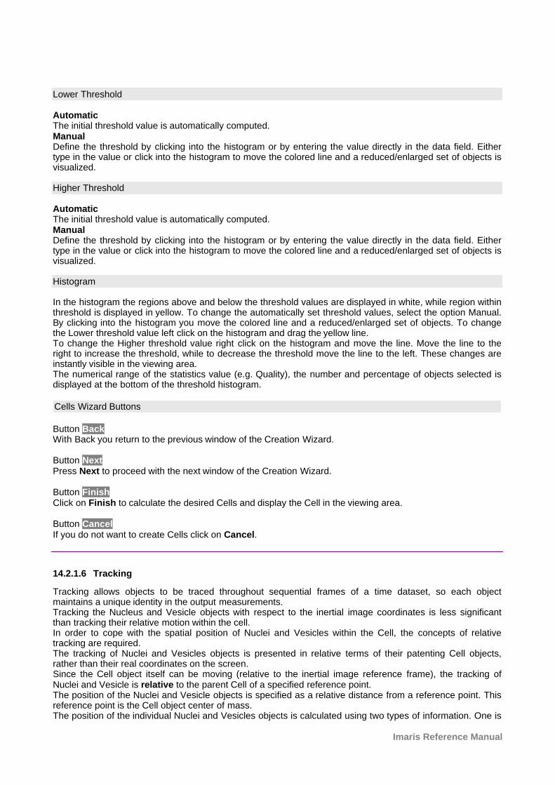
Imaris Reference Manual
Lower Threshold
AutomaticThe initial threshold value is automatically computed.ManualDefine the threshold by clicking into the histogram or by entering the value directly in the data field. Eithertype in the value or click into the histogram to move the colored line and a reduced/enlarged set of objects isvisualized.
Higher Threshold
AutomaticThe initial threshold value is automatically computed.ManualDefine the threshold by clicking into the histogram or by entering the value directly in the data field. Eithertype in the value or click into the histogram to move the colored line and a reduced/enlarged set of objects isvisualized.
Histogram
In the histogram the regions above and below the threshold values are displayed in white, while region withinthreshold is displayed in yellow. To change the automatically set threshold values, select the option Manual.By clicking into the histogram you move the colored line and a reduced/enlarged set of objects. To changethe Lower threshold value left click on the histogram and drag the yellow line. To change the Higher threshold value right click on the histogram and move the line. Move the line to theright to increase the threshold, while to decrease the threshold move the line to the left. These changes areinstantly visible in the viewing area.The numerical range of the statistics value (e.g. Quality), the number and percentage of objects selected isdisplayed at the bottom of the threshold histogram.
Cells Wizard Buttons
Button BackWith Back you return to the previous window of the Creation Wizard.
Button NextPress Next to proceed with the next window of the Creation Wizard.
Button FinishClick on Finish to calculate the desired Cells and display the Cell in the viewing area.
Button CancelIf you do not want to create Cells click on Cancel.
14.2.1.6 Tracking
Tracking allows objects to be traced throughout sequential frames of a time dataset, so each objectmaintains a unique identity in the output measurements.Tracking the Nucleus and Vesicle objects with respect to the inertial image coordinates is less significantthan tracking their relative motion within the cell. In order to cope with the spatial position of Nuclei and Vesicles within the Cell, the concepts of relativetracking are required.The tracking of Nuclei and Vesicles objects is presented in relative terms of their patenting Cell objects,rather than their real coordinates on the screen. Since the Cell object itself can be moving (relative to the inertial image reference frame), the tracking ofNuclei and Vesicle is relative to the parent Cell of a specified reference point. The position of the Nuclei and Vesicle objects is specified as a relative distance from a reference point. Thisreference point is the Cell object center of mass.The position of the individual Nuclei and Vesicles objects is calculated using two types of information. One is
© Bitplane 2010
the absolute position of the selected object in terms of the inertial image reference coordinates and the otheris the absolute position of the parent Cell object center. The relative Nuclei and Vesicles object’s position iscalculated by subtracting these two positional differences and is then tracked. This concept of relative tracking allows direct measurements and statistical data comparison betweenmoving cells to be calculated.
Track (Autoregressive Motion)
Track Nucleus
Select this option and the Nucleus objects will be tracked.
Track Vesicles
Select this option and the Vesicles objects will be tracked.
Autoregressive MotionThis algorithm models the motion of each object as an autoregressive AR1 process. This model isappropriate if object perform any kind of continuous motion. The AR1 model looks back to one time-point,and predicts that the object will move again the same distance and in the same direction. The user specifiesthe value of maximum distance. This value is the distance in which the object is allowed to deviate from thepredicted position. Some changes in direction are tolerated because of the value of the maximum distanceparameter, and because the AR1 algorithm performs correlations only to one previous time-point.
Parameters
Max Distance CellThe value of the Max Distance specifies the maximum distance that a track Cell object could possibly movebetween two consecutive time points. This parameter disallows connections between a Cell and a candidatematch if the distance between the predicted future position of the Cell and the candidate position exceeds themaximum distance.
Max Relative Distance NucleusThe value of the Max Distance specifies the maximum distance that a track Nucleus could possibly movebetween two consecutive time points, relative to the parenting Cell center of mass.
Max Relative Distance VesiclesThe value of the Max Distance specifies the maximum distance that a track Vesicles could possibly movebetween two consecutive time points, relative to the parenting Cell center of mass.
Options
It can happens that the object segmentation fails for some time points. This can break a Track apart into twoTracks. The gap-closing algorithm tries to continue the movement of a disappearing object and connects theTracks if it reappears.
Close GapSelect this option and the gap-closing algorithm is implemented.Max Gap SizeThe maximum gap size value defines the maximum consecutive time points until the object re-appears.
Cells Wizard Buttons
Button BackWith Back you return to the previous window of the Creation Wizard.
Button NextPress Next to proceed with the next window of the Creation Wizard.
Button FinishClick on Finish to calculate the desired Cells and display the Cell in the viewing area.
Imaris Reference Manual
Button CancelIf you do not want to create Cells click on Cancel.
14.2.1.7 Classify Tracks
The Tracks filtering is incorporated into the creation process. This tab only appears, if Track Cells (overTime) is checked (Algorithm).
A filtering allows the removal of objects that would interfere with interpretation of results.
The Filter Type and its values define the section of interest, from this selection, which includes or excludesobjects based on a range of criteria. Select the filter type by selecting a variable from the drop-down list, andthen define the filter values, which will then limit the selection just to those objects that meet the set upcriteria. In Imaris you can choose two filter values, a Lower and a Higher filter value. The two filter values separate the data into three regions: above the higher value, below the lower value, andthe region in between. Objects with the relevant properties below the Lower filter value and objects with theproperties exceeding the Higher filter value will be excluded, and only those objects with qualities inside thedefined interval will be considered.
Please note if the value of the Lower filter value is set to be higher than that of the Higher filter value, theselected objects will be outside the defined interval. Only those objects meeting all the filter criteria areinteractively shown and instantly highlighted in the viewing area.
By using multiple filter types, more than one criterion can be specified for the data analyses.
Filters
Add ButtonTo add a new filter, click on the button Add and choose one of the Filter Types from the drop-down menu.The new filter appears in the list.Delete ButtonSelect a filter in the list with a left mouse click and click on this button to delete the filter.
Filter Type
Select in the drop down list the filter you want to apply.
Filter category
A Category identifies, gathers and summaries a set of statistical values calculations of a particular ObjectType. Statistical values associated with one object type are grouped in one category. Each category has anassociated button with graphical indications of Category type.In Imaris there are following Filter Categories: Surface , Surface Tracks , Spots , Spots Tracks ,
Dendrites , Dendrites Tracks , Filament , Filament Tracks , Spines , Spine Tracks , Point ,
Point Tracks , Cell , Cell Tracks , Nucleus , Nucleus Tracks , Vesicle and Vesicles Tracks
. These buttons allow you to choose the Category and determines the list of displayed statistical values.Clicking the button selects the corresponding category (the category button turns black) and the list ofstatistical values is displayed according to the selection.To remove the category from the list, re-click on the Category button. Re-clicking on the category buttonde-selects Category and removes the selected statistical values from the list (turns the category button into alight gray color).
The exclamation mark sign indicates that the listed statistical parameter does not contain any value.
Compact Lower and Upper Threshold
© Bitplane 2010
Activating/deactivating the Lower or Upper threshold option is done by clicking on the or button. The
Red button indicates that the threshold option is currently inactive, while the green button indicates anactive threshold.In order to activate the threshold option, click on the red button. To deactivate the threshold, click on thegreen circle again.
Automatic/Manual A/M buttonThe Automatic/Manual A/M button provides a single interaction point for the direct choice of the thresholdvalue adjustment.
When the lower/upper threshold values are not activated (the red button ) the corresponding A/M button islight gray indicating that threshold adjustment is unavailable. When the lower/upper threshold option is
activated (the green button ), the corresponding A/M button turns black.
After the first threshold activation, as a default, an Automatic threshold value is activated . Clicking onthe Automatic/Manual button allows you to switch between an Automatic and a Manual threshold adjustmentmode. The A/M button provides a visual feedback as an indication of the selected threshold adjustment
mode. Clicking on the A/M button changes the appearance of the A/M button form indicating an
activated Automatic threshold to indicating a Manual threshold. Clicking on the histogram automatically activates a Manual threshold adjustment.
Lower Threshold
AutomaticThe initial threshold value is automatically computed.ManualDefine the threshold by clicking into the histogram or by entering the value directly in the data field. Eithertype in the value or click into the histogram to move the colored line and a reduced/enlarged set of objects isvisualized.
Higher Threshold
AutomaticThe initial threshold value is automatically computed.ManualDefine the threshold by clicking into the histogram or by entering the value directly in the data field. Eithertype in the value or click into the histogram to move the colored line and a reduced/enlarged set of objects isvisualized.
Histogram
In the histogram the regions above and below the threshold values are displayed in white, while the regionwithin the threshold is displayed in yellow. To change the automatically set threshold values, select the optionManual. By clicking into the histogram you move the colored line and a reduced/enlarged set of objects. Tochange the Lower threshold value left click on the histogram and drag the yellow line. To change the Higher threshold value right click on the histogram and move the line. Move the line to theright to increase the threshold, while to decrease the threshold move the line to the left. These changes areinstantly visible in the viewing area.The numerical range of the statistics value (e.g. Quality), the number and percentage of objects selected(e.g. Tracks) is displayed at the bottom of the threshold histogram.
Surfaces Wizard Buttons
Button BackWith Back you return to the previous window of the Creation Wizard.
Button NextPress Next to proceed with the next window of the Creation Wizard.
Button FinishClick on Finish to calculate the desired Surfaces and display the Surfaces in the viewing area.
Imaris Reference Manual
Button CancelIf you do not want to create Surfaces click on Cancel.
14.2.1.8 Complete ROI
This tab only appears, if Process entire Image finally is checked (Algorithm).
Region of Interest
The parameters you have set up will now be used to compute Spots (and Tracks) for the entire data set.Depending on the size of the data set this may take a while.
Surfaces Wizard Buttons
Button BackWith Back you return to the previous window of the Creation Wizard.
Button FinishClick on Finish to end the calculation and display the results in the viewing area.
Button CancelIf you do not want to create Surfaces click on Cancel.
14.2.2 Tab Settings
On the tab Settings you can choose the rendering methods and adjust the rendering quality to produce fasterperformance of the display.
Object Type
A choice of Object types is presented. For time series images the choice of the Object Type is in the dropdown list. After choosing the Object type, a selection of the Setting Tab is listed.
Cell visibleThis option shows or hides the Cell objects in the viewing area.Nucleus visibleThis option shows or hides the Nucleus objects in the viewing area.
Cell and Nuclei Style
Ortho SlicerOrtho Slicer represents an orthogonal plane (orthogonal to the coordinate axis of the data set) that can bemoved within the data set. Three orthoslicer planes show their intersection with a plane perpendicular to twoof the coordinate axesChange the slice direction if required by selecting the adequate plane.The check buttons labeled as XY, XZ and YZ direction, are used to select the visibility of the correspondingslice.
The position of slices can be changed in the viewing area. Switch the pointer to the Select mode and thenclick on the plane and drag it to a new position.
Dataset visible (slicers only)This option is available only if orthoslicer options are selected. When this option is selected the dataset isshown on the slicers in addition to the Cell/Nucleus objects.
Oblique slicerThe Oblique Slicer represents a plane that can be freely moved and rotated within the data set and allows the
© Bitplane 2010
user to look inside any object. The Oblique Slicer consists of a colored frame with a white double rod in themiddle.The position of the Oblique Slicer can be changed. Choose the pointer mode Select, highlight the ObliqueSlicer in the viewing area and click on the bigger diameter rod. It will appear highlighted as it is selected,allowing you to move it and to set the Oblique Slicer to the required position.The Oblique Slicer can be rotated around the x-, y-, and the z-axes. In the Select mode click the smallerdiameter rod and it will be highlighted as it is selected. To rotate the Oblique Slicer, move the smaller rod.
MIP RenderingThis option visualizes the cells and nuclei as Maximum Intensity Projection (MIP). A Maximum IntensityProjection is a method for 3D data visualization. The MIP Rendering method uses the intensity value of thebrightest voxel along the ray path traced from the viewpoint to the plane of projection.
Volume RenderingThis option performs a three-dimensional volume rendering and illustrates a 3D structure of the objects.Volume rendering enhances 3D structures compared to slice display and facilitates understanding of spatialrelationship.
Vesicles Style/Quality
On the tab Settings you can adjust the rendering style or quality.
Center PointsThis option displays the Vesicles as center points.
OffSelect this option to disable the visualization of the Vesicles.
SphereSelect this option to display the Vesicles as spheres.
Radius Scale boxThe size of the Vesicles can be changed via the Radius Scale box.
The Render QualityThe Render Quality is adjustable using the slider. When the number of Vesicles is very large, adjust theRender Quality,to produce a faster display performance.
Cell/Nucleus/Vesicles Tracks
Tracks Style/Quality
The box Style/Quality has settings that determine the display of the connections between the Track objects.
CylinderSelect this option to display the tracks connections as cylinders.
LineSelect this option to display the tracks connections as lines.
OffSelect this option to disable the visualization of the Tracks.
WidthDiameter/Render qualityDepending on the previous selection you can either adjust the width of the line or the diameter of the cylinder.
DisplacementCheck the box Displacement to show the displacement of a Track as an arrow. To assign another color, clickon the Color symbol to open the Color Editor.
Imaris Reference Manual
Radius ScaleAn Edit field for the displacement vector radius.
Dragon TailCheck the box Dragon Tail and instead of showing a Track in its entire length on all time points, only parts ofit are shown depending on the selected time points. The number of time points is determined with the sliderposition.
SliderThe Dragon Tail length can be adjusted using the slider. The slider determines the number of time points inthe length of the Dragon Tail.
14.2.3 Tab Creation
Rebuild
Imaris stores the list of operations and the mapping of parameters. Select from the list, which step of the CellCreation Wizard you want to re-enter.
For details please refer to chapter:Menu Surpass - Cells - AlgorithmMenu Surpass - Cells – Tracking
Button Rebuild ObjectsClick on this button to start the rebuild.
Creation Parameters
The Creation Wizard saves parameters and processing instructions so that the Cell computation can berepeated for the same region, a different region, or the entire image. The Creation Parameters are listed asthe table.
Button Add to Batch
The Add to Batch button places the command into the Batch coordinator with all the adjusted parametervalues.
14.2.4 Tab Edit
Once the Cell creation wizard is completed, use these buttons for manual editing of the Cell objects. It allowsyou:1. To import Surfaces or Spots and incorporate them in the Cells analysis.2. To export objects from the Cells.3. To clear the selection or delete all selected component of the cell object.
Import
Import Surface to CellTo import the Surface as the Cell or the Nuclei Objects, click on this button. The window, Import to CellObject, will appear.
Import Spots to VesiclesTo import the Spots as the Vesicles, click on this button. The window, Import to Cell Object, will appear.
Import to Cell Object window
Choose one of the objects from the drop-down menu. Choose how the selected object type is to be importedand specify the selection and the time. The Surface can be imported either as the Cell or the Nuclei.
© Bitplane 2010
The Spots can be imported only as the Vesicles.The user can decide either to import the Selection or the All objects of the specified component. The time point of the object selected can be imported either as the Current time point or the All timepoints.
Export
SelectionThe Selection checkbox is used to export only the currently selected object.
All Timepoints The All Timepoints checkbox is used to export the object for all time points.
Export Cells to Surface With a click on this button you export the Cell objects to a Surface object. The Surpass Tree list is
automatically updated with the new item with the automatically generated name Cells n Cell Export. Theexported objects can be then manually edited.
Export Nuclei to SurfaceWith a click on this button you export the Nuclei objects to a Surface object. The Surpass Tree list is
automatically updated with the new item with the automatically generated name Cells n Nucleus Export.The exported objects can be then manually edited.
Export Vesicles to Spots With a click on this button you export the Vesicles to a Spots object. The Surpass Tree list is automatically
updated with the new item with the automatically generated name Cells n Vesicles Export. The exportedobjects can be then manually edited.
Full Export With a click on this button you export all the Cell objects. The Cell and Nuclei objects are exported toSurface, while the Vesicles objects are exported to Spots.The Surpass Tree list is updated and three new surpass objects are generated (two Surface items and oneSpot item) with the automatically generated names Cells n object-name Export. Pressing this button hasthe same effect as pressing the three buttons above.
Process Selection
Clear ButtonClick this button to clear the current object selection.
Delete ButtonClick on this button to delete all the currently selected components.
All actions in the Draw , Edit and Edit Tracks tabs can be Undone/Redone by selecting the Undo/Redo command or by pressing Ctrl+Z/Ctrl+Y.
14.2.5 Tab Edit Tracks
Table Layout
In the track editor a horizontal line represents each track. Each horizontal line is composed of circles,representing objects, and line segments which connect a sequence of objects.The first row of the track-editing table displays the timeline. Each number represents a time point in theseries.The second row of the track-editing table displays the object name. Multiple object types can be tracked easily since every object type appears in different colors.
Object ID
Imaris Reference Manual
If the mouse pointer is on the object, a tooltip appears that identifies the object ID. The ID numbers of theobjects are sequentially ordered column-wise from the top to the bottom of the table. The object maintains itsunique ID number independent of the track being allocated to. If the mouse pointer is on the connection, a tooltip appears that identifies the track ID number.
Interactive Selection
When you click on an individual row, the editing table highlights the corresponding object in the image.Similarly, by clicking on an object within the image (while the pointer is in Select mode) the correspondingtrack (row in table) is highlighted. In addition, the Statistical and Filter Tab can be used to select tracks for editing. By clicking on the value inthe statistical table, the corresponding object in the viewing area as well as the track in the track-editing tableis selected.For multiple selections press Ctrl+click (Mac: Command+click).
Visualization options
ZoomMoving the mouse up and down while pressing the middle mouse button allows you to see more ("zoom out")or less ("zoom in") of the track-editing table. Using the mouse wheel will have the same affect.PanTo move the track editing table click and hold the right mouse button while dragging the mouse. Release theright mouse button to place the table on the chosen location.
Time indicatorThe first row of the track-editing table displays the timeline. Each number represents a time point in theseries. The current time point is indicated by vertical line highlighted with in current selection color.
To modify the time point, do one of the following: 1. Moving the slider in the Time bar modifies its position in time and changes the time point in the trackeditor. 2. Clicking on the time point within the track-editing table automatically moves the time line indicator to thecorresponding point.Double clicking on the time indicator, fixes the position of the current time point at the center of thetrack-editing table, regardless of the selected zoom or pan options)
Editing
Track Editor has several features that help you modify your tracks
Add tracks
To set the starting point of a new connection first you have to select the object. Shift+left-click followed by a mouse movement on the object creates the new connection. To establish a connection, drag the edge to the target object. If valid, the target object is highlighted (red). Release the mouse button and the line segment clips automatically onto the new object, creating a newconnection between the two objects.
Please note: The new connection is only possible between the objects of the same type. If you release themouse button without being on a target object, the edge will disappear and a new connection will not beestablished.
A connection between objects of the same time point is also invalid.
Delete Tracks Edges
TracksSelect the track and press backspace to delete the whole track.
ConnectionsTo delete the connection, select the connection and press shift-click. The selected connection is deleted.
© Bitplane 2010
The process of deleting the connection splits the track. The first track part remains with the same ID numberand stops at the time point of the deletion. The second part consists of the remaining deleted objects and theconnections between them. It is automatically shifted to the bottom of the track-editing table and assigned anew track ID number.
Connect unconnected components
Manually added, or previously untracked objects are displayed as separated circles. The procedure ofcreating new connections and connecting the objects is unchanged.
Show selection (working set)
This option allows you to work on subset of tracks.
Connect Track Button
Click this button to connect two existing tracks. Select two Spots in two different tracks at the subsequenttime points (just one Spot per time point) and click on the button Connect Track. The connection isautomatically created between all selected objects.
Disconnect Track Button
Select a object and click on the button Disconnect Track. The connection from the selected object to the nextobject in time sequence is deleted.
Correct Drift
If you have an object drift (e.g. a cell drift) during the image acquisition you can use the Correct Drift button tocorrect the drift for the whole data set.
The ImarisTrack tracks all objects in an image, even the objects that should be stationary.The Correct Drift function gives the user the opportunity:
1) to specify the tracks related to the stationary objects 2) to assign these objects as stationary objects and 3) to adjust the position of the rest of the image objects based on this selection.
As a result of drift correction, the entire image is transformed in such a way that the selected objects remainstationary and within the new image each objects’ position (changes) based on the correct draft algorithm.Within the new image, the true movement of the objects can be then detected relative to the stationaryobjects.
In the accordance with the selected for Result DataSets options. the new image coordinates are calculatedand displayed.
To make the Drift Correction on the data set the following steps are completed:· Select the tracks associated with the stationary objects· Select the algorithm for drift correction · Select the option for the Result data sets · Verify the selection and click on the OK button.
Please note: The drift correction changes the data set.
Based on the provided the track sub-selection the algorithm determines the new objects position for all timepoints.If the tracks are selected, the algorithm will be performed on the sub selection. Otherwise, every track of theimage is considered for calculations.
Algorithms
The Drift Correction is calculated based on the two algorithms, Translation and translation and rotation.
Imaris Reference Manual
Translation
Upon translation, the object position is transformed to a straight line of identical orientation. Within the sametime point the relative distance of the objects is preserved.
Translation and rotation
Upon translation and rotation, the object position is transformed based on the image polar coordinates.Within the same time point the relative distance of the objects is preserved.
Please note: The number of the selected tracks affects the algorithm calculation.
Selection of a single track gives a complete description of a translation.Selection of a two tracks gives a minimum description of a translation and rotation algorithm (planar rotation). A better fit between the time points is achieved when three or more tracks are selected.
Result DataSet size
After completion of the drift correction, the algorithm uses the final position of the initial and resulting imageto create a final image. The new image coordinates are calculated in accordance with the size of the originaland new image.Select the Result data set option to determine which new image part will be displayed.
Crop largest common region
The final image will be the size of the common overlap between the original and the drift corrected image.Areas of the image that have been shifted outside these boundaries (to allow alignment) will be cropped fromthe final result.
New size equal to current size The final image will be the same size as the original image. Areas of the image that have been shiftedoutside these boundaries (to allow alignment) will be cropped from the final result.
Include entire result
The final image will be the size of the combined area of the original and corrected image.Selecting the appropriate Result dataset size may speed up the data visualization. This is especiallyimportant with (with large data sets.)
Correct spots positions
Activate this parameter and the spots are automatically re-positioned after the drift correction. If this option isnot activated only the image volume is aligned.
All actions in the Draw , Edit and Edit Tracks tabs can be Undone/Redone by selecting the Undo/Redo command or by pressing Ctrl+Z/Ctrl+Y.
14.2.6 Tab Filter
Please note: Before using you have to add a filter to the list (see below: button Add)!
The Filter Type and its values define the section of interest, from this selection, which includes or excludesobjects based on a range of criteria. Select the filter type by selecting a variable from the drop-down list, andthen define the filter values, which will then limit the selection just to those objects that meet the set upcriteria. In Imaris you can choose two filter values, a Lower and a Higher filter value. The two filter values separate the data into three regions: above the higher value, below the lower value, andthe region in between. Objects with the relevant properties below the Lower filter value and objects with theproperties exceeding the Higher filter value will be excluded, and only those objects with qualities inside thedefined interval will be considered.
© Bitplane 2010
Please note if the value of the Lower filter value is set to be higher than that of the Higher filter value, theselected objects will be outside the defined interval. Only those objects meeting all the filter criteria areinteractively shown and instantly highlighted in the viewing area.
By using multiple filter types, more than one criterion can be specified for the data analyses.
Filters
Add ButtonTo add a new filter, click on the button Add and choose one of the Filter Types from the drop-down menu.Select the filtering type to be used in order to classify objects and specify the measurement of the criteria tobe used. The new filter appears in the list.
Delete ButtonSelect a filter in the list with a left mouse click and click on this button to delete the filter.
Filter Type
Select in the drop down list the filter you want to apply.
Filter category
A Category identifies, gathers and summaries a set of statistical values calculations of a particular ObjectType. Statistical values associated with one object type are grouped in one category. Each category has anassociated button with graphical indications of Category type.In Imaris there are following Filter Categories: Surface , Surface Tracks , Spots , Spots Tracks ,
Dendrites , Dendrites Tracks , Filament , Filament Tracks , Spines , Spine Tracks , Point ,
Point Tracks , Cell , Cell Tracks , Nucleus , Nucleus Tracks , Vesicle and Vesicles Tracks
. These buttons allow you to choose the Category and determines the list of displayed statistical values.Clicking the button selects the corresponding category (the category button turns black) and the list ofstatistical values is displayed according to the selection.To remove the category from the list, re-click on the Category button. Re-clicking on the category buttonde-selects Category and removes the selected statistical values from the list (turns the category button into alight gray color).
The exclamation mark sign indicates that the listed statistical parameter does not contain any value.
Compact Lower and Upper Threshold
Activating/deactivating the Lower or Upper threshold option is done by clicking on the or button. The
Red button indicates that the threshold option is currently inactive, while the green button indicates anactive threshold.In order to activate the threshold option, click on the red button. To deactivate the threshold, click on thegreen circle again.
Automatic/Manual A/M buttonThe Automatic/Manual A/M button provides a single interaction point for the direct choice of the thresholdvalue adjustment.
When the lower/upper threshold values are not activated (the red button ) the corresponding A/M button islight gray indicating that threshold adjustment is unavailable. When the lower/upper threshold option is
activated (the green button ), the corresponding A/M button turns black.
After the first threshold activation, as a default, an Automatic threshold value is activated . Clicking onthe Automatic/Manual button allows you to switch between an Automatic and a Manual threshold adjustmentmode. The A/M button provides a visual feedback as an indication of the selected threshold adjustment
mode. Clicking on the A/M button changes the appearance of the A/M button form indicating an
activated Automatic threshold to indicating a Manual threshold. Clicking on the histogram automatically activates a Manual threshold adjustment.
Imaris Reference Manual
Lower Threshold
AutomaticThe initial threshold value is automatically computed.ManualDefine the threshold by clicking into the histogram or by entering the value directly in the data field. Eithertype in the value or click into the histogram to move the colored line and then a reduced/enlarged set ofobjects are visualized.
Higher Threshold
AutomaticThe initial threshold value is automatically computed.ManualDefine the threshold by clicking into the histogram or by entering the value directly in the data field. Eithertype in the value or click into the histogram to move the colored line and then a reduced/enlarged set ofobjects are visualized.
Histogram
In the histogram the regions above and below the threshold values are displayed in white, while the regionwithin the threshold is displayed in yellow. To change the automatically set threshold values, select the optionManual. By clicking into the histogram you move the colored line and the reduced/enlarged set of objects. Tochange the Lower threshold value left click on the histogram and drag the yellow line. To change the Higher threshold value right click on the histogram and move the line. Move the line to theright to increase the threshold and to decrease the threshold move the line to the left. These changes areinstantly visible in the viewing area.The numerical range of the statistics value (e.g. Quality)and the number and percentage of objects that fallinto the particular filtering class are displayed at the bottom of the threshold histogram.
Duplicate Selection to New Surfaces ButtonClick on this button and all selected objects are copied to a new group. The new group displays in theSurpass Tree.
14.2.7 Tab Statistics
Cells statistics are automatically computed. For the statistical values please refer to the chapter Menu Edit -Preferences... - Statistics - Cells. The Statistics tab collects and displays the image's statistical values inImaris. The Statistics tab enables us to understand and compare different datasets through summarizedstatistical values and graphical data presentations. Several types of statistical tools enable convenient organization and analysis of heterogeneous statisticaldata. The Statistics View is configured as follows: a) Overall b) Detailedc) SelectionIn the statistical dataset the first column contains the name of the variable, followed by columns withcalculated statistical data. Corresponding statistical variable values are presented in rows. To sort the columns click on the arrow in column heading. Click again to reverse the sort.
Overall Tab
Output of the Overall statistics provides an overview of the image's single determining variables. Onlystatistics that are not measured on a per-object basis are displayed here.
Category
A Category identifies, gathers and summaries a set of statistical values calculations of a particular ObjectType.
© Bitplane 2010
Statistical values associated with one object type are grouped in one category. Each category has anassociated button with graphical indications of Category type.In Imaris there are following Filter Categories: Surface , Surface Tracks , Spots , Spots Tracks ,
Dendrites , Dendrites Tracks , Filament , Filament Tracks , Spines , Spine Tracks , Point ,
Point Tracks , Cell , Cell Tracks , Nucleus , Nucleus Tracks , Vesicle and Vesicles Tracks
. These buttons allow you to choose the Category and determines the list of displayed statistical values.Clicking the button selects the corresponding category (the category button turns black) and the list ofstatistical values is displayed according to the selection.To remove the category from the list, re-click on the Category button. Re-clicking on the category buttonde-selects Category and removes the selected statistical values from the list (turns the category button into alight gray color).
The exclamation mark sign indicates that the listed statistical parameter does not contain any value.
Detailed Tab
Tables in the Detailed Tab are showing a statistical data collected from all of the objects within the image. Apull down list offers three types of Detailed statistical calculations: Specific ValuesAverage ValuesAll Values
Time Plots The values displayed are always for the current time point. Selecting a variable that changes over timecreates a plot of selected values as a time function. The statistical variable value is plotted on the verticalaxis and the time is plotted on the horizontal axis. The current time point is indicated with a black vertical line.Each time value is displayed as a point. Click inside the plot and move the time line. Moving the line changesthe time point. Altering the time point changes the variable value and the image.Multiple value selection, available by Ctrl+ click, will plot a superimposed second selected value over the firstone.
Interactive two-way SelectionA click on an individual row of the table highlights the corresponding object in the image. Similarly, by clickingon an element in the image (while the pointer is in Select mode) the corresponding row in table will behighlighted. A possibility of multiple selections is available by pressing Ctrl+click (Mac: Command+click).
Specific Values In the Specific Values, a second pull down list at the top of the window displays available specific statisticalvalues. Select the variable and a list of values will be displayed. Object Statistical Annotation option is available for Specific values parameters.
Average valuesThe Average table contains values determined on the basis of all values within a set of the selected variable.Columns are labeled as follows:Min (Minimum)- the smallest value within a set of values of the selected variable Max (Maximum)- the largest value within a set of values of the selected variable Mean – value of the sum of all values divided by number of values within a set Std Dev (Standard deviation)- a measure of the values distribution around the mean values Median- the middle value of the sorted set of variablesSum- the sum of all values within a variable setCount- number of values within a setUnit- variable unit Level/Distance
The black line on the time plot indicates where the mean value lies, the red indicates the median, the lightgray area shows the range between the min and max values and dark gray region labels the standarddeviation range with error bars.
Statistical variable classification: 1. Statistical variables associated with objects (Cells, Nucleus, Vesicles -volume, area, intensity values,
Imaris Reference Manual
position, speed, displacement) have values at every time point. Therefore for these variables the Averagevalues are displayed per time point. Changing the time points, statistical variable values and images areconsequently changed.2. Statistical values with data associated with Tracks (track duration, track volume mean, track displacementlength, track intensity) are not time dependent.
All valuesIf the option All values is selected for the detailed tab, all values will be displayed. Even though this option isalways readily available, it is discouraged to use it in order to avoid data clutter.Object Statistical Annotation option is available for Specific values parameters.
Selection Tab
Statistical tables for a selected object will be displayed. Change to the pointer mode Select and click on animage element that has been detected/segmented. A possibility of multiple selections is available byCtrl+click (Mac: Command-click).A pull down list offers three types of statistical calculations from a Selection:Specific ValuesAverage ValuesAll Values
Time Plots The values displayed are always for the current time point. Selecting a variable that changes over timecreates a plot of selected values as a time function. The statistical variable value is plotted on the verticalaxis and the time is plotted on the horizontal axis. The current time point is indicated with a black vertical line.Each time value is displayed as a point. Click inside the plot and move the time line. Moving the line changesthe time point. Altering the time point changes the variable value and the image.Multiple value selection, available by Ctrl+ click, will plot a superimposed second selected value over the firstone.
Interactive two-way SelectionA click on an individual row of the table highlights the corresponding object in the image. Similarly, by clickingon an element in the image (while the pointer is in Select mode) the corresponding row in table will behighlighted. A possibility of multiple selections is available by pressing Ctrl+click (Mac: Command+click).
Specific valuesIn the Specific Values, a second pull down list at the top of the window displays available specific statisticalvalues. Select the variable and a list of values will be displayed.Object Statistical Annotation option is available for Specific values parameters.
Average valuesThe Average table contains values determined on the basis of all the values within a set of the selectedvariables for the selected image element(s). For further explanation see Average values Detailed statistics.This choice only makes sense in the context of the Selection Tab if you have selected more than oneelement from the image.
The black line on the time plot indicates where the mean value lies, the red indicates the median, the lightgray area shows the range between the min and max values and dark gray region labels the standarddeviation range with error bars.
All valuesIf the option All values is selected, all statistical values will be displayed for the selected image element. Object Statistical Annotation option is available for Specific values parameters.
Buttons Overview
PC: Mac: Select Cells Left-click Click Select multiple Cells Ctrl + left-click Command + click
© Bitplane 2010
Buttons at the bottom of the Statistics tab
Button Settings -Configure a List of visible statistics values. Click on the button Settings and you switch to the window Preferences - Statistics - Cells.
Button Search - Search by object ID.Type in the object ID in the data field. Click on the button Search. · Highlights the object in the viewing area· Highlights the object on the Detailed Tab· Displays of the values on the Selection Tab
Button Cells - Duplicate Selection to new Cells.Click on this button and all selected elements are copied to a new Cell. The new Cell appears in the SurpassTree, and the old one is hidden, but still available.
Button Statistical Annotation Click this button and an object statistical annotation will be automatically generated in the viewing area. Thisoption is available only when Specific or All Values are selected
Button Export - Export Statistics on Tab Display to File. Only the statistics that are shown within the current tab will be exported.
Button Export - Export selected Data for plottingExports the selected statistical value for plotting. The selected value has to be time dependent.With a click on the button Export the Export Statistics window opens. Select the file type (CommaSeparated Values *.csv, Excel file *.xls, or Excel XML *.xlm). If you select MS Excel as file type, the programstarts automatically.
Button Export - Export All Statistics to File. All of the statistics (that are enabled in the statistics settings) will be exported.With a click on the button Export the Export Statistics window opens. Select the file type (CommaSeparated Values *.csv, Excel file *.xls, or Excel XML *.xlm). If you select MS Excel as file type, the programstarts automatically and the sheets show up one after another (this will take several seconds).
See also:Menu Edit - Preferences... - Statistics - Cells
14.2.7.1 Statistical Annotations
Statistical annotations provides the opportunity to view and annotate image objects with the statistical datavalues. Using this function, the individual objects in an image are labeled with the specified statistical valuesand the statistical data is displayed directly in the viewing area Imaris objects can be labeled with a set of any number of the user-defined statistical values.The Statistical Annotation button provides a convenient interface to label the object with the statisticaldata. Click this button and an object statistical annotation will be automatically generated in the viewingarea. The selected object is annotated for all time points with the specified statistical values.
How to add Statistical Annotation
In the Statistical tab choose the Detailed or Selection Tab. In the viewing area select the object or group of objects. Change to the pointer mode Select and click on animage object that has been detected/segmented. For multiple selections press Ctrl+click (Mac:Command-click)In the Detailed or Selection Tab a pull down list offers Specific Values or All values as types of statisticalparameters. Select the statistical value associated with the particular object type you are working with.Press the Statistical Annotation button .
In the viewing area the object label appears showing selected statistical values as a statistical annotation.
The statistical annotation shows by default the name of the selected statistical parameter and its value.
Imaris Reference Manual
The color white displays the text of annotations associated with statistical values.
For a single object, all selected statistical parameters are placed in the same annotation box. Once the objectis labeled, selecting the additional statistical parameter updates the object statistical annotation; the newparameter and its value is added in the viewing area.If the image is a time series, the statistical annotation will be visible in the viewing area for all time points.Selecting a statistical variable that changes over time creates an statistical annotation that consequentlychanges with every time point.The statistical annotation displays values always for the current time point.
The InPress options will allow you to modify and specify the contents and format of the object labels.
To modify and adjust the statistical label click on the Icon InPress , press Ctrl + Shift + P, or in the menubar select File – InPress.
14.2.8 Tab Color
Choice of the Object type is presented in a drop down window. Select Cell, Cell Tracks, Nucleus, NucleusTracks, Vesicle or Vesicle Tracks.Depending on the chosen object type selection of the variables is listed.
The tree color types are available:BaseStatistics CodedTime Mapped
14.2.8.1 Tab Color-Base
RGB
The RGB color model is an additive color model in which Red, Green and Blue are combined together toreproduce an array of colors. The color values may be changed either by clicking on the color wheel to selecta color or by direct numeric entry for the Red, Blue or Green component (values range from 0 to 1).
Light reflection
Quality of the object material is further characterized by reflection properties. Diffusion- diffuses reflection of a matte, uneven material.Specular- defines reflection of highly reflective materials. The brighter a specular map is, the more shine isapplied to the object. Default setting has no specular intensity.Emission- light emitted from the material defines the self-illumination. Default setting emits no light.
Transparency
Transparency- defines the amount of light allowed to pass through an object. Click this tool to change thepercentage from 0% (complete opacity) to 100% (complete image transparency).
Palette
Palette- this option provides a system of preset colors organized into color schemes. In the Palette, colors are labeled and grouped together. The scrolling window contains the 14 colorcombination groups (Custom, artdeco, autumn, glass, metal, neon, rococo, santafe, sheen, silky, spring,summer, tropical, winter). Examples of colors in a selected group are displayed in the attached rectangulararea. If a custom color has been defined on the RGB tab, it can be added to the Custom palette with the Addto Palette button. After being added, these color choices are stored and can be used with other Imarisobjects.
14.2.8.2 Tab Color-Statistics Coded
Depending on the chosen object type the Statistical variable selection is listed in the drop down window. Forexample, if Cell/Nuclei/Vesicle is chosen as the Object type, available Statistical data will be theCell/Nuclei/Vesicle linked variable. Similarly, variables for Tracks will be listed, if the object type is selected tobe Tracks.
© Bitplane 2010
Statistics Colorbar Properties
Statistics colorbar are displayed in the viewing area. The upper one is the colorbar range forCel/Nucleus/Vesicles and lower one is the colorbar for the Tracks.
Show ColorbarCheck the box to see the statistics colorbar in the viewing area.
Show TitleCheck this box to see the title in the statistics colorbar.
Show RangeCheck this box to see the range in the statistics colorbar.
Font color in colorbar is adjustable by selecting a color within the color map.
Colormap
Button ResetClick the Reset button to set the image back to the original values.
Button Load …Click on the button Load to display the Import Color Table File color window. Enter the path and therequested File name and/or File type and click Open. The selected file is loaded and displayed.
Colormap range
Colormap range-specify the limits for the colorbar. Min - lower color limitMax - upper color limitButton AutoClick the button Auto and the system detects the real min and max values and sets the Max. and Min. limitsautomatically to these values.
Transparency
Transparency defining amount of light allowed to pass through. Click this tool to change the percentagefrom 0% (complete opacity) to 100% (complete image transparency).
14.2.8.3 Tab Color-Time Mapped
This option is only available when Tracks (see above) is selected as an Object Type. The color range for theTracks goes from blue to white to the range of time points.
Transparency
Transparency defining amount of light allowed to pass through. Click this tool to change the percentagefrom 0% (complete opacity) to 100% (complete image transparency).
14.3 Clipping Plane
The Clipping Plane cuts away objects on one side of the plane. It can be freely moved and rotated in thescene and allows you to look inside any object. The Clipping Plane consists of a colored frame with a whitedouble rod in the middle.To change the position and orientation of the Clapping Plane in the View Area the Pointer must be in Selectmode.
How to Add a new Clipping Plane?
· Select menu Surpass - Clipping Plane.
Imaris Reference Manual
The Surpass Tree list is automatically updated and in the Clipping Plane - Properties the Settings parameterare displayed. The Clipping Plane is displayed in the viewing area.
To clip another object, this object must be placed behind the clipping plane within the Surpass Tree. It mustbe in the same group as the Clipping Plane and it must be placed below the Clipping Plane.
Change Position of Clipping Plane
The position of the Clipping Plane can be changed. Choose the pointer mode Select, highlight the ClippingPlane in the viewing area and click on the bigger diameter rod. It will turn colored as it is selected, move it toset the Clipping Plane to the required position.
Rotate Clipping Plane around Axes
The Clipping Plane can be rotated around the x-, y-, and the z-axes. In Select mode click the smallerdiameter rod. It will turn colored as it is selected, move it to rotate the Clipping Plane.
See also:Surpass View - Overview - Camera Toolbar - Pointer (Mode Select)
14.3.1 Tab Settings
Position
Button RecenterThe Clipping Plane center is moved to the data set center.
Orientation
Button YZ PlaneButton XZ PlaneButton XY PlaneThe Clipping Plane is oriented parallel to either the yz-plane, the xz-plane or the xy-plane.
Button FlipClick on the Flip button to flip the orientation of the clipping plane.
Configuration
Button StoreButton RecallAfter changing the position and/or orientation of the Clipping Plane, the new configuration can be stored byclicking on the Store button. The position previously stored can be recalled by selecting the Recall button.
Camera
Button Orthogonal ViewThe camera is set to a position which is perpendicular to the Clipping Plane.
Show FrameTo make the frame visible, check this box.
Perpendicular Movement
The pointer must be in the pointer mode Select. Place the mouse within the image. To change the orientationof the rod press the Ctrl button. The Clipping Plane is moved in the directions parallel to the plane.
See also:Surpass View - Overview - Camera Toolbar - Pointer (Mode Select)
© Bitplane 2010
14.3.2 Mouse & Keyboard PC
Clipping Plane Mouse & Keyboard Functions
Left-click on plane & drag Move plane to desired positionLeft-click on the bigger diameter rod & drag Move plane to desired positionLeft-click on the smaller diameter rod & dragRotate plane to desired position
See also:Addendum - Mouse & Keyboard PC
14.3.3 Mouse & Keyboard Mac
Clipping Plane Mouse & Keyboard Functions
Click on plane & drag Move plane to desired positionClick on the bigger diameter rod & drag Move plane to desired positionClick on the smaller diameter rod & drag Rotate plane to desired position
See also:Addendum - Mouse & Keyboard Mac
14.4 External Object
Surpass provides the ability to import External objects (both, non-Imaris and Imaris objects) and display themconcurrently with a Surpass object for comparison.
Only the External objects with the extension *.iv (Inventor file) or with extension *.vrml (VRML2 files) can beimported.
The imported External objects can be rotated, scaled and translated.
For example, previously calculated Surfaces, which have been exported as Inventor files, can be imported toanother data set.
How to Add a new External Object?
· Select menu Surpass - External Object.
The Surpass Tree list is automatically updated and in the External object - Properties the Settings parameterare displayed.
See also:Menu Surpass - Export Selected Objects ...
14.4.1 Tab Settings
The object properties area displays a number of parameters for the positioning and display of the Externalobject. The following display/handling options can be checked:
Box HandleThe object shows a surrounding box with handles. These handles allow to transform/distort the object in thex-, y-, and z-direction.
TrackballThe object shows surrounding circular lines. These lines allow rotation of the External object in any direction.
File Path FieldDisplay of the file path (to load the object, see below).
Imaris Reference Manual
Button Load...To select and load a data set as a External object click on the button Load... and the Load External ObjectFile window is displayed. Select the file to be loaded as External object. The External object will be onlyloaded if the selected files have the extension *.iv (Inventor file) or *.vrml (VRML2 files). Click on the buttonOpen.
Button Reset Size and LocationClicking this button sets the External object back to its original size and position before any translational,scaling or rotational operations have been performed.
Fix RatioIf this option is checked and if scaling is performed on the External object by entering a value, the samescaling factor is applied to all three dimensions.
Position/Scaling
The following positional/scaling options are available:
TranslationUse these fields to move the External object in the x-, y-, or z-direction.
RotationUse this field to rotate the External object around the x-, y-, or z-axis.
ScalingUse this field to scale the External object in one of the dimensions (or all together if Fix Ratio, see above, ischecked). Fix Ratio is only valid with this method of scaling.
See also:Menu Surpass - Export Selected Objects ...
14.4.2 Tab Color
Color Tab edit, manage and assign material colors of an Object.
RGB
The RGB color model is an additive color model in which Red, Green and Blue are combined together toreproduce an array of colors. The color values may be changed either by clicking on the color wheel to selecta color or by direct numeric entry for the Red, Blue or Green component (values range from 0 to 1).
Light reflection
Quality of the object material is further characterized by reflection properties. Diffusion- diffuses reflection of a matte, uneven material.Specular- defines reflection of highly reflective materials. The brighter a specular map is, the more shine isapplied to the object. Default setting has no specular intensity.Emission- light emitted from the material defines the self-illumination. Default setting emits no light.
Transparency
Transparency- defines the amount of light allowed to pass through an object. Click this tool to change thepercentage from 0% (complete opacity) to 100% (complete image transparency).
Palette
Palette- this option provides a system of preset colors organized into color schemes. In the Palette, colors are labeled and grouped together. The scrolling window contains the 14 colorcombination groups (Custom, artdeco, autumn, glass, metal, neon, rococo, santafe, sheen, silky, spring,summer, tropical, winter). Examples of colors in a selected group are displayed in the attached rectangular
© Bitplane 2010
area. If a custom color has been defined on the RGB tab, it can be added to the Custom palette with the Addto Palette button. After being added, these color choices are stored and can be used with other Imarisobjects.
14.4.3 Mouse & Keyboard PC
External Object Mouse & Keyboard Functions
Left-click white box & drag Scale object from centerLeft-click white box + Ctrl & drag Scale object from opposite cornerLeft-click trackball & drag Rotate objectShift + left-click trackball & drag Set up a rotation axis
See also:Addendum - Mouse & Keyboard PC
14.4.4 Mouse & Keyboard Mac
External Object Mouse & Keyboard Functions
Click white box & drag Scale object from centerClick white box + Ctrl & drag Scale object from opposite cornerClick trackball & drag Rotate objectShift + click trackball & drag Set up a rotation axis
See also:Addendum - Mouse & Keyboard Mac
14.5 Filament
General
In IMARIS the dendritic trees are represented by a set of vertices and edges. The Vertex is drawn as anode or a dot and defines the center axis of the dendrites. An edge is presented as a line connecting twovertices. The entity of vertices and edges is referred to as filament graph. Parts of the filament graph can be classified as spines either collectively, based on some statistical values, orindividually by the user, by determined specifications.Starting, ending and branching vertices are classified into dendrite beginning point, dendrite branchpoint, dendrite terminal point, spine attachment point, spine branch point, and spine terminal pointdepending on their position in the graph (refer to the picture below). Segments are defined as the collection of edges between two starting, ending, or branching vertices.Segments are classified either as dendrite segments or spine segments. In a dendrite the edge is called adendrite edge, in a spine it is called a spine edge.
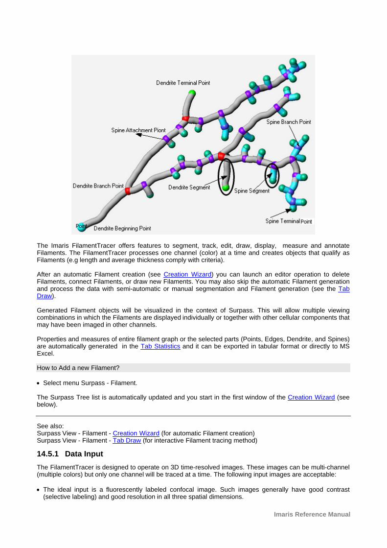
Imaris Reference Manual
The Imaris FilamentTracer offers features to segment, track, edit, draw, display, measure and annotateFilaments. The FilamentTracer processes one channel (color) at a time and creates objects that qualify asFilaments (e.g length and average thickness comply with criteria).
After an automatic Filament creation (see Creation Wizard) you can launch an editor operation to deleteFilaments, connect Filaments, or draw new Filaments. You may also skip the automatic Filament generationand process the data with semi-automatic or manual segmentation and Filament generation (see the TabDraw).
Generated Filament objects will be visualized in the context of Surpass. This will allow multiple viewingcombinations in which the Filaments are displayed individually or together with other cellular components thatmay have been imaged in other channels.
Properties and measures of entire filament graph or the selected parts (Points, Edges, Dendrite, and Spines)are automatically generated in the Tab Statistics and it can be exported in tabular format or directly to MSExcel.
How to Add a new Filament?
· Select menu Surpass - Filament.
The Surpass Tree list is automatically updated and you start in the first window of the Creation Wizard (seebelow).
See also:Surpass View - Filament - Creation Wizard (for automatic Filament creation)Surpass View - Filament - Tab Draw (for interactive Filament tracing method)
14.5.1 Data Input
The FilamentTracer is designed to operate on 3D time-resolved images. These images can be multi-channel(multiple colors) but only one channel will be traced at a time. The following input images are acceptable:
· The ideal input is a fluorescently labeled confocal image. Such images generally have good contrast(selective labeling) and good resolution in all three spatial dimensions.
© Bitplane 2010
· 3D images can also be acquired using a standard microscope (non-confocal) equipped with a CCDcamera and a stepper motor. Non-confocal optical arrangements do not provide resolution along theoptical axis which is why every single plane consists of in-focus components and out-of-focus components.These images require deconvolution prior to tracing. The technique of deconvolution uses informationabout the imaging process (the point spread function) to remove the out-of-focus components from everysection.
· Finally there are 3D images taken in transmission light microscopy. Staining is usually less specific than inthe fluorescent case and it will be more difficult to automatically segment the Filament. Deconvolution canalso be applied to transmission images although - theoretically - its performance is weaker than in thefluorescent case.
14.5.2 Creation Wizard
The automatic filament graph compilation (creation) is guided by a wizard-like user interface and consistsessentially of five steps.
· Select the appropriate algorithm (or quit the automatic filament creation and draw the filamentsinteractively).
· Define a Region of Interest · Select source channel and do some pre-processing.· Segmentation to specify filamentous and non filamentous parts.· Graph compilation and finishing.
The Creation Wizard allows to go forth and back until the optimal parameters are found.
See also:Surpass View - Filament - Creation Wizard - AlgorithmSurpass View - Filament - Creation Wizard - PreprocessingSurpass View - Filament - Tab Draw (for interactive filament tracing method)
14.5.2.1 Algorithm
In this first window of the Creation Wizard you decide, if you want to go for an fully automated filamentcreation using one of the two predefined algorithms (AutoPath-no loops or Threshold-loops, see below); or ifyou want to draw the filaments interactively. If you do not want to use the automatic filament creation wizard select the Skip automatic creation, editmanually button.
Skip automatic creation, edit manually Button Terminates the creation wizard and activates the interactive filament tracing method.
Select Algorithm
The automatic filament creation provides two algorithms to choose from:AutoPath (no loops)Threshold (loops)
AutoPath (no loops)The automated AutoPath Algorithm:· Produces a tree-like filament· Is based on local intensity contrast· Connects large start- and small end-points
If you select this algorithm please refer to chapter: Surpass View - Filament - Creation Wizard - AutopathAlgorithm (no loops)
Threshold (loops)The Threshold based Algorithm:
Imaris Reference Manual
· Produces a filament with loops· Is based on an absolute intensity threshold· Thinning to a skeleton
If you select this algorithm please refer to chapter Surpass View - Filament - Creation Wizard - ThresholdAlgorithm (loops)
Calculate Diameter of Filament from Image
Check this box and the Filament diameter is calculated based on the image data. Un-check the box and the Filament diameter will taper smoothly from the starting point to the end points.
Region of Interest-ROI
A Region of Interest (ROI) is a selected sub-region of an image identified for particular processes andanalyzes. Defining and processing ROI allows other parts of an image to be unchanged.
Build Filament for All Time Points
The option is available only if you work with a time data set. Check the box if you want to create a filamentover all time points.
Track (over time)
Check this box if you want to track Filament over time, for details please refer to the tab Tracking.
Filament Wizard Buttons
Button Next Press Next to proceed with the next of the Creation Wizard.
Button FinishPress Finish and based on the selected algorithm (see above) Imaris runs through all parameters (comingon the following windows of the Creation Wizard) using the default settings. At the end of the calculation theFilaments are displayed in the viewing area.
Button CancelClick on this button if you do not want to use the automatic graph compilation. Use instead the interactivefilament tracing method. The parameters on the tab Settings are displayed in the properties area. Pleaserefer to chapter Surpass View - Filament - Tab Draw to adjust the parameters.
14.5.2.2 Autopath Algorithm (no loops)
The Autopath (no loops) algorithm consists of the following steps:
Region of InterestDendrite Points DiameterClassify Dendrite PointsDendrite DiameterSpine Points DiameterClassify Spine PointsSpine DiameterTrackingFinish
14.5.2.3 ROI
Region of Interest 1
Here you define the region of interest (ROI). Parameters such as width, height and location of the ROI areused to directly specify the area to work on.
© Bitplane 2010
X, Y, Z, TimeMin, Max, SizeMinimum, maximum and Size of ROI coordinate values, can be specified either by entering the value in thevalue fields or changing the values by clicking on up-and down arrows at the right hand side of the valuefields.Alternatively the location and size of the ROI can be adjusted directly in the viewing area. Size of the ROI:1. Click on the ROI preview rectangle arrows (change to the pointer mode Select) 2. Drag the arrows to define new coordinates for X ,Y and Z. Location of the ROI: 1.Click inside the ROI preview rectangle 2. Drag the entire rectangle (with mouse button held) to the chosen image location. The numbers in the value fields are updated automatically.
Memory Usage:Display of the memory usage for the image size within the ROI.
Regions of Interest
To select a particular ROI, left-click on its name in the list and the selected ROI will be highlighted within animage and its properties can be adjusted.
Button AddClick on this button and a new region of interest appears in the list. To adjust this ROI you have to select theROI with a left mouse click.
Button DeleteSelect a ROI in the list with a left mouse click and click on this button to delete the ROI.
Total Memory Usage:Display of the memory usage for the image size within the ROI.
Filament Wizard Buttons
Button BackWith Back you return to the previous window of the Creation Wizard.
Button NextPress Next to proceed with the next window of the Creation Wizard.
Button FinishClick on Finish to calculate the desired Filament and display the Filament in the viewing area.
Button CancelIf you do not want to create Filament automatically click on Cancel.
14.5.2.4 Dendrite Points Diameter
Select Source Channel
Select the respective source channel, from which the Dendrite structure is to be computed.
Starting Points
Detect a new starting point -a new starting point of the filament will be determined, based on the valuegiven for the largest diameter.
(largest Diameter: e.g. Dendrite Beginning)Enter a value of the maximum (largest) diameter of dendrite to specify the Starting point diameter.
Seed Points
Imaris Reference Manual
(Thinnest Diameter e.g. Dendrite Ending)Enter a value of the minimum (smallest) diameter of dendrite to specify the Seed points diameter.
Rebuild Options
As part of the rebuilding process in step three of the Creation wizard – Dendrite Point Diameter, a new optionexists for selecting a Starting Point.
Use Existing Dendrite
Use Existing Dendrite- the previously determined dendrite points will be used in the creation of new startingpoint. Therefore, in the next creation step (Starting point threshold) an option for Manual Start point editing in(shift+right click) will not be available.
Filament Wizard Buttons
Button BackWith Back you return to the previous window of the Creation Wizard.
Button NextPress Next to proceed with the next window of the Creation Wizard.
Button FinishPress Finish and Imaris runs through all parameters (coming on the following windows of the CreationWizard) using the default settings. At the end of the calculation the Filaments are displayed in the viewingarea.
Button CancelClick on this button if you do not want to use the automatic graph compilation. Use instead the interactivefilament tracing method. The parameters on the tab Settings are displayed in the properties area. Switch tothe tab Draw and please refer to chapter Surpass View - Filament - Tab Draw to adjust the parameters.
By reentering the Creation Wizard, either after selecting Rebuilding Algorithm or for Processing additionalROI(s) a new option exists for selecting a Starting Point.
See also:Surpass View - Filament - Tab SettingsSurpass View - Filament - Tab Draw (for interactive filament tracing method)
14.5.2.5 Classify Dendrite Points
Thresholds are used to classify the detected dendrite’s starting points and seed points.The detected dendrite starting point(s) are visualized in the image by different colors. The respectivehistograms are displayed. The threshold can be set manually or automatically.
Compact Lower and Upper Threshold
Activating/deactivating the Lower or Upper threshold option is done by clicking on the or button. The
Red button indicates that the threshold option is currently inactive, while the green button indicates anactive threshold.In order to activate the threshold option, click on the red button. To deactivate the threshold, click on thegreen circle again.
Automatic/Manual A/M buttonThe Automatic/Manual A/M button provides a single interaction point for the direct choice of the thresholdvalue adjustment.
When the lower/upper threshold values are not activated (the red button ) the corresponding A/M button islight gray indicating that threshold adjustment is unavailable. When the lower/upper threshold option is
© Bitplane 2010
activated (the green button ), the corresponding A/M button turns black.
After the first threshold activation, as a default, an Automatic threshold value is activated . Clicking onthe Automatic/Manual button allows you to switch between an Automatic and a Manual threshold adjustmentmode. The A/M button provides a visual feedback as an indication of the selected threshold adjustment
mode. Clicking on the A/M button changes the appearance of the A/M button form indicating an
activated Automatic threshold to indicating a Manual threshold. Clicking on the histogram automatically activates a Manual threshold adjustment.
Starting Points Threshold
Display of the starting points threshold and the respective histogram. The threshold can be adjusted byentering a new value in the data field or by moving the colored threshold line (click & drag) in the histogram.The updated points are visualized in the viewing area.
Manual Starting Points addition/deletion in Creation Wizard
Manual addition of starting points in the filament structure is available by pressing Shift+ right-click. Shift+right-click on an existing filament start point (created either automatically or manually added) and theselected starting point will be deleted.
Seed Points Threshold
Display of the end points threshold and the respective histogram. The threshold can be adjusted by enteringa new value in the data field or by moving the colored threshold line (click & drag) in the histogram. Theupdated points will be visualized in the viewing area.
Manual Seed Points Addition/Deletion in Creation Wizard
Manual Addition of Seed points in the filament structure is available by Shift+ left-click. Shift+ left-click on anexisting point, (created either automatically or manually added) and the selected point will be deleted.
Remove Seed Points Around Starting Point(s)
Check the box and all seed points located within the radius of the sphere centered at the starting point areremoved. The boundary of the sphere is defined by the value Diameter of Sphere Region(s).
Diameter of Sphere Region(s)Enter the diameter of the sphere centered at the beginning point. Default value set to twofold of the startingpoints diameter.
Filament Wizard Buttons
Button BackWith Back you return to the previous window of the Creation Wizard.
Button NextPress Next to proceed with the next window of the Creation Wizard.
Button FinishClick on Finish to calculate the desired Filament and display the Filament in the viewing area.
Button CancelIf you do not want to create a Filament automatically click on Cancel.
14.5.2.6 Dendrite Diameter
The option is only available if in the step Algorithm the Calculate Diameter form the image is selected.The threshold value is based on the local contrast and the respective histogram is displayed.
Imaris Reference Manual
The defined threshold value is used for the dendrite diameter calculation.
Compact Lower and Upper Threshold
Activating/deactivating the Lower or Upper threshold option is done by clicking on the or button. The
Red button indicates that the threshold option is currently inactive, while the green button indicates anactive threshold.In order to activate the threshold option, click on the red button. To deactivate the threshold, click on thegreen circle again.
Automatic/Manual A/M buttonThe Automatic/Manual A/M button provides a single interaction point for the direct choice of the thresholdvalue adjustment.
When the lower/upper threshold values are not activated (the red button ) the corresponding A/M button islight gray indicating that threshold adjustment is unavailable. When the lower/upper threshold option is
activated (the green button ), the corresponding A/M button turns black.
After the first threshold activation, as a default, an Automatic threshold value is activated . Clicking onthe Automatic/Manual button allows you to switch between an Automatic and a Manual threshold adjustmentmode. The A/M button provides a visual feedback as an indication of the selected threshold adjustment
mode. Clicking on the A/M button changes the appearance of the A/M button form indicating an
activated Automatic threshold to indicating a Manual threshold. Clicking on the histogram automatically activates a Manual threshold adjustment.
The effect of changing the threshold value is directly visible in the viewing area.
Algorithm
The Algorithm provides two methods to calculate dendrite diameter.
Shortest distance from distance map The dendrite diameter is calculated as the shortest distance between dendrite center point and dendritesurface.
Approximate circle of cross section areaThe diameter of the approximate circle of cross-sectional area is determined as a value of the dendritediameter.
Filament Wizard Buttons
Button BackWith Back you return to the previous window of the Creation Wizard.
Button NextPress Next to proceed with the next window of the Creation Wizard.
Button FinishClick on Finish to calculate the desired Filament and display the Filament in the viewing area.
Button CancelIf you do not want to create a Filament automatically click on Cancel.
14.5.2.7 Spine Points Diameter
Spine
Detect Spines Check this box to Optimize the Creation wizard for Spine Detection; creating the highly branched filamentstructure.Un-check the box Detect Spines and the Spine channel selection and the Seed Points diameter are disabled.Spines detection and creation are not performed in the following creation procedure.
© Bitplane 2010
Select Source Channel
Select the respective source channel, from which the spines are to be computed. The default channel is thesame as for the dendrite detection.
Seed Points
(Thinnest Diameter e.g. Small Spine Head)Enter a value of the minimum (smallest) diameter of spine head to specify the Seed points diameter.
Maximum Length
The Maximum Length is estimated spine length, the length from the dendrite center to the furthest Spineseed point.
Allow Branch SpinesCheck the Allow Branch Spines option to allow formation of the spines's bifurcation points. To formbifurcation point the two spine's vertices have to be in the vicinity of 1 voxel.
Filament Wizard Buttons
Button BackWith Back you return to the previous window of the Creation Wizard.
Button NextPress Next to proceed with the next window of the Creation Wizard.
Button FinishClick on Finish to calculate the desired Filament and display the Filament in the viewing area.
Button CancelIf you do not want to create a Filament automatically click on Cancel.
14.5.2.8 Classify Spine Points
The option is only available if in the step Points Diameter the Detect Spine option is selected.
Spine
Seed Points Threshold
Thresholds is used to classify the spines seed points. The detected Spine seed points are visualized in theimage. The respective histogram is displayed. The threshold can be set manually or automatically.
Compact Lower and Upper Threshold
Activating/deactivating the Lower or Upper threshold option is done by clicking on the or button. The
Red button indicates that the threshold option is currently inactive, while the green button indicates anactive threshold.In order to activate the threshold option, click on the red button. To deactivate the threshold, click on thegreen circle again.
Automatic/Manual A/M buttonThe Automatic/Manual A/M button provides a single interaction point for the direct choice of the thresholdvalue adjustment.
When the lower/upper threshold values are not activated (the red button ) the corresponding A/M button islight gray indicating that threshold adjustment is unavailable. When the lower/upper threshold option is
activated (the green button ), the corresponding A/M button turns black.
Imaris Reference Manual
After the first threshold activation, as a default, an Automatic threshold value is activated . Clicking onthe Automatic/Manual button allows you to switch between an Automatic and a Manual threshold adjustmentmode. The A/M button provides a visual feedback as an indication of the selected threshold adjustment
mode. Clicking on the A/M button changes the appearance of the A/M button form indicating an
activated Automatic threshold to indicating a Manual threshold. Clicking on the histogram automatically activates a Manual threshold adjustment.
The threshold can be adjusted by entering a new value in the data field or by moving the colored thresholdline (click & drag) in the histogram. The updated points are visualized in the viewing area.The effect of changing the threshold value is directly visible in the viewing area.
Filament Wizard Buttons
Button BackWith Back you return to the previous window of the Creation Wizard.
Button NextPress Next to proceed with the next window of the Creation Wizard.
Button FinishClick on Finish to calculate the desired Filament and display the Filament in the viewing area.
Button CancelIf you do not want to create a Filament automatically click on Cancel.
14.5.2.9 Spine Diameter
The option is only available if in the step Points Diameter the Detect Spine option is selected.The threshold value is based on the local contrast and the respective histogram is displayed.The defined threshold value is used for the Spine diameter calculation.
Compact Lower and Upper Threshold
Activating/deactivating the Lower or Upper threshold option is done by clicking on the or button. The
Red button indicates that the threshold option is currently inactive, while the green button indicates anactive threshold.In order to activate the threshold option, click on the red button. To deactivate the threshold, click on thegreen circle again.
Automatic/Manual A/M buttonThe Automatic/Manual A/M button provides a single interaction point for the direct choice of the thresholdvalue adjustment.
When the lower/upper threshold values are not activated (the red button ) the corresponding A/M button islight gray indicating that threshold adjustment is unavailable. When the lower/upper threshold option is
activated (the green button ), the corresponding A/M button turns black.
After the first threshold activation, as a default, an Automatic threshold value is activated . Clicking onthe Automatic/Manual button allows you to switch between an Automatic and a Manual threshold adjustmentmode. The A/M button provides a visual feedback as an indication of the selected threshold adjustment
mode. Clicking on the A/M button changes the appearance of the A/M button form indicating an
activated Automatic threshold to indicating a Manual threshold. Clicking on the histogram automatically activates a Manual threshold adjustment.
The effect of changing the threshold value is directly visible in the viewing area.
Algorithm
The Algorithm provides two methods to calculate Spine diameter.
Shortest Distance From Distance Map The Spine diameter is calculated as the shortest distance between dendrite center point and spine surface.
© Bitplane 2010
Approximate Circle of Cross Section AreaThe diameter of the approximate circle of cross-sectional area is determined as a value of the spinediameter.
Filament Wizard Buttons
Button BackWith Back you return to the previous window of the Creation Wizard.
Button NextPress Next to proceed with the next window of the Creation Wizard.
Button FinishClick on Finish to calculate the desired Filament and display the Filament in the viewing area.
Button CancelIf you do not want to create a Filament automatically click on Cancel.
14.5.2.10 Tracking
The filament object consists of a set of the dendrites, the spine points and the connection between them.Tracking allows objects to be traced throughout sequential frames of time dataset. Each object maintains anunique identity in the output measurements.
This tab only appears, if the Track Filament (over Time) is checked (Algorithm Settings).
The Filament tracking tab provides Autoregressive Motion algorithms, which model the filament movement. The algorithm utilizes the object’s direction and speed information from one single time point to predict thebest potential object position at the next time point.Based on the tracking of the entire Filament graph, the algorithm predicts the future positions of the DendriteBeginning Point, Branching and Terminal Points as well as the Spine Attachments, Spine Terminal PointsBased on these predicted positions, the best matches to the candidate points can be determined. Thealgorithms use a Linear Assignment algorithm and a Total Cost function to find the best track connections.The total cost computation is based on the change in distance.
Autoregressive Motion
This algorithm models the motion of the filament graph’s center of gravity as an autoregressive AR1 process. The AR1 model looks back to previous time-point, and predicts that the filament object will move again thesame distance and in the same direction. The user-specified maximum distance value is the distance inwhich object is allowed to deviate from the predicted position. Some changes in direction are tolerateddepending on the setting of the Max. Dist. parameter. and because the AR1algoritham calculates the positionbased on only one time-point.
Max Distance
The value of the Max Distance specifies the maximum distance between a predicted object location and itsactual location for two consecutive time points. This parameter does not allow connections between aFilament graph and a candidate match when the distance between the predicted future position of theFilament graph and the candidate position exceeds the maximum distance.It can happen that the object segmentation fails for some time points, which can break a Track apart into twoTracks. The gap-closing algorithm tries to continue the movement of a disappearing object and connects theTracks if they reappear.
Close Gap
Select this option and the gap-closing algorithm will be implemented.
Max Gap Size
Imaris Reference Manual
The maximum gap size value defines the maximum of the consecutive time points until the objectre-appears.
Track Dendrites
Select this option and the Dendrite points will be tracked.When the Track Dendrite option is not selected the drop-down list remains inactive.
From the drop-down list you can select the type of Dendrite points to be tracked. There are two options:· Dendrite Branch Points · Dendrite Terminal Points
Please note: The tracking of the Dendrite Beginning point is automatically computed based on the tracking ofthe entire Filament structure.
Enable track
Check the box to enable the selected Dendrite points to be traced.
Please note: The spine tracking options are only available if the spines have been previously created.
Track Spines
Select this option and the Spine points will be tracked.From the drop down list select the type of Spine points to be tracked. There are three options:· Spine Attachment Points· Spine Branch Points · Spine Terminal Points
Enable track
Check the box to enable the selected Spine points to be traced.
Close Gap
Select this option and the gap-closing algorithm will be implemented.
Max Gap Size
The maximum gap size value defines the maximum of the consecutive time points until the objectre-appears.
Filament Wizard Buttons
Button BackWith Back you return to the previous window of the Creation Wizard.
Button FinishClick on Finish to calculate the desired Filament and display the Filament in the viewing area.
Button CancelIf you do not want to create a Filament automatically click on Cancel.
14.5.2.11 Finish ROI Processing
The selected parameters will be used to complete the computation of a Filament structure in an image. Byselecting one of six finishing options a Filament structure will be created in the following ways:
1. Entire Image in This Time Point - the entire image is processed with the same set of parameters usedfor the ROI processing and the filament structure is created for the entire image and the selected time point.Only available if you work with a time data set.
© Bitplane 2010
2. Additional Region in This Time Point - re-enters creation process (in step two-ROI) and uses the samethe same set of parameters for a new ROI to create the filament structure only for the selected time point.Only available if you work with a time data set.
3. Additional Regions in Other Time Point - re-enters creation process (in step two-ROI) and uses thesame set of parameters for a new ROI to create the filament structure for the new time point. Only available ifyou work with a time data set. When the data set contains multiple time points, the Filament Creation Wizardcan create Filament objects for each time point with the same set of parameters.
4. Current Region in All Time Points - re-enters creation process (in step two-ROI) and uses the samecreation algorithm for a new ROI to creates the filament structure for all time points. Only available if youwork with a time data set. When the data set contains multiple time points, the Filament Creation Wizard cancreate Filament objects for each time point with the same set of parameters.
5. Entire Image in All Time Points- the entire image is processed with the same parameters used for theROI processing and the filament structure is created for the entire image and all time points. Only available ifyou work with a time data set. When the data set contains multiple time points, the Filament Creation Wizardcan create Filament objects for each time point with the same set of parameters.
6. All Done- creates a filament structure only within an ROI.
Please refer to Tab Creation. In step three of the Creation wizard – Point Diameter, an option exists forselecting a Starting Point (Use existing filament or Detect a new starting point).
Note: The Use Existing Filament option requires that the new ROI overlaps with some portion of the existingfilament.
Filament Wizard Buttons
Button BackWith Back you return to the previous window of the Creation Wizard.
Button NextPress Next to proceed with the next window of the Creation Wizard.
Button FinishClick on Finish to calculate the desired Filament and display the Filament in the viewing area.
Button CancelIf you do not want to create a Filament automatically click on Cancel.
14.5.2.12 Threshold Algorithm (loops)
The threshold (loops) algorithm consists of the following steps:PreprocessingSegmentationGraph CompilationFinish
14.5.2.13 Preprocessing
Source Channel
Select the respective source channel, from which the Filament structure is to be computed.
Feature Preprocessing
Enable Feature PreprocessingCheck the box and the following parameters are adjustable. Un-check the box and the following parametersare grayed. Preprocessing is not necessary if the data is already deconvolved or if the noise has alreadybeen removed by a Gaussian filter. The preprocessing will be applied to the source channel and the result
Imaris Reference Manual
will be added as new Filament Working channel in the Display Adjustments.
Appr. Filament DiameterAn approximate minimal Filament diameter has to be provided.
Preserve EdgesYou can also enable an edge preserving preprocessing to maintain filamentous structures.
Before continuing you can inspect the result of the previous step with any viewer of Imaris: Slice, Section,Gallery, Easy3D, Surfaces etc.
Filament Wizard Buttons
Button BackWith Back you return to the previous window of the Creation Wizard.
Button NextPress Next to proceed with the next window of the Creation Wizard.
Button FinishPress Finish and Imaris runs through all parameters (coming on the following windows of the CreationWizard) using the default settings. At the end of the calculation the Filaments are displayed in the viewingarea.
Button CancelClick on this button if you do not want to use the automatic graph compilation. Use instead the interactivefilament tracing method. The parameters on the tab Settings are displayed in the properties area. Switch tothe tab Draw and please refer to chapter Surpass View - Filament - Tab Draw to adjust the parameters.
See also:Menu Edit - Show Display AdjustmentMenu Image Processing - Thresholding - Connective BaselineSurpass View - Filament - Tab Draw (for interactive filament tracing method)
14.5.2.14 Segmentation
Segmentation
Fill Cavities (fully enclosed volumes)Check this box to avoid hollow regions. These regions would be enclosed by a Filament mesh, which is notdesired in most of the cases.
Connective BaselineType in two values for the lower threshold (colored line) and upper threshold (red line). You can also click intothe histogram. Left mouse button for lower, right mouse button for upper threshold or you can click & dragthe respective line.
Simple thresholding methods classify voxels purely based on a single intensity value. This approach oftendoes not lead to good results because the staining, the illumination, and the detection operate within aprecision range. The connective thresholding scheme takes care of this and searches for object voxels usingan intensity range rather than a single intensity.
You must provide two threshold values. The lower threshold (colored line) is the intensity below which a voxelis recognized as part of the background, the upper threshold (red line) is the minimal intensity for a voxel tobe part of the Filament object. Voxels with an intensity value between the two thresholds are treated as partof the Filament object if and only if they are connected to a voxel within intensity above the upper threshold("double thresholding" with "feature-AND").
The result of the segmentation process described above is a clean image where the non-zero voxels aredescribing the objects (Filaments and some non-filamentous structures). Because such a description of thedata is not suitable for morphometric analysis the structures are converted. Graph compilation is a process
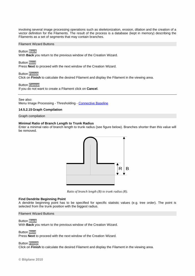
© Bitplane 2010
involving several image processing operations such as skeletonization, erosion, dilation and the creation of avector definition for the Filaments. The result of the process is a database (kept in memory) describing theFilaments as a set of segments that may contain branches.
Filament Wizard Buttons
Button BackWith Back you return to the previous window of the Creation Wizard.
Button NextPress Next to proceed with the next window of the Creation Wizard.
Button FinishClick on Finish to calculate the desired Filament and display the Filament in the viewing area.
Button CancelIf you do not want to create a Filament click on Cancel.
See also:Menu Image Processing - Thresholding - Connective Baseline
14.5.2.15 Graph Compilation
Graph compilation
Minimal Ratio of Branch Length to Trunk RadiusEnter a minimal ratio of branch length to trunk radius (see figure below). Branches shorter than this value willbe removed.
R B
Ratio of branch length (B) to trunk radius (R).
Find Dendrite Beginning PointA dendrite beginning point has to be specified for specific statistic values (e.g. tree order). The point isselected from the trunk position with the biggest radius.
Filament Wizard Buttons
Button BackWith Back you return to the previous window of the Creation Wizard.
Button NextPress Next to proceed with the next window of the Creation Wizard.
Button FinishClick on Finish to calculate the desired Filament and display the Filament in the viewing area.
Imaris Reference Manual
Button CancelIf you do not want to create a Filament click on Cancel.
14.5.2.16 Finish
Finish
To validate the automatically generated graph and the prior segmentation, you can inspect the result togetherwith numerous Surpass modules: Ortho Slicer, Volume, Surfaces etc. You can optionally superimpose thesegments with the original slices of the image stack using Imaris OrthoSlicers. OrthoSlicers are planes,which are perpendicular to any of the three spatial axes and extend throughout the entire image volume.
Build Filaments for all Time PointsOnly available if you work with a time data set. When the data set contains multiple time points, the FilamentCreation Wizard can create Filament objects for each time point with the same set of parameters. They willbe visible within the Surpass Tree. However the 3D Filament graph is only visible according to its time point.
Delete Working ChannelThe Filament Working channel can be kept for other use. Principally it is not needed any more when finishingthe Filament graph.
Filament Wizard Buttons
Button BackWith Back you return to the previous window of the Creation Wizard.
Button NextThis button is grayed in the last window of the Creation Wizard.
Button FinishClick on Finish to end the calculation and display the results in the viewing area.
Button CancelIf you do not want to create Filaments click on Cancel.
14.5.3 Filament Properties
When the creation process is finished, the tab Create disappears while some other property Tabs appear.They allow the manipulation of the filament graph:
Tab CreateOnly appears when you Add a new Filament.
Tab SettingsChange Filament appearance and inspect selection statistics.
Tab CreationRe-enter the creation process.
Tab DrawManually draw filaments and connections.
Tab EditSelect automatically filament parts and delete or smooth them.
Tab StatisticsInspect all statistic values.
© Bitplane 2010
Tab ColorChange the color appearance (material) of the filament.
See also:Surpass View - Filament (Add a new Filament)Surpass View - Filament - Tab SettingsSurpass View - Filament - Tab CreationSurpass View - Filament - Tab DrawSurpass View - Filament - Tab EditSurpass View - Filament - Tab StatisticsSurpass View - Filament - Tab Color
14.5.4 Tab Settings
On the tab Settings you can edit and adjust the display options.Select Filament to adjust quality and style of the filament graph. Select Filament Tracks and you can edit and adjust settings that determine the display of connectionsbetween the Track filament graphs.
14.5.4.1 Filament
Style
LineCylinderConeThe visualization of the graph is done as lines with a specified thickness (pixel), as cylinders (with a defineddiameter), or cones (using the measured graph diameter).
Show Dendrites
Check the box in the heading to highlight dendrite points in the filament. The special points are highlightedwith color-coded spheres.
Beginning PointCheck this box to highlight the dendrite beginning points.
Branch PointsCheck this box to highlight the dendrite branch points.
Terminal PointsCheck this box to highlight the dendrite terminal points.
Show Spines
Check the box in the heading to highlight spine points in the filament. The special points are highlighted withcolor-coded spheres.
Attachment PointsCheck this box to highlight the spine attachment points.
Branch PointsCheck this box to highlight the spine branch points.
Terminal PointsCheck this box to highlight the spine terminal points.
Imaris Reference Manual
Render Quality
With the slider you can adjust the render quality of the filament. Moving the slider to the left reduces therender quality, moving it to the right increase render quality.
14.5.4.2 Filament Track
Tracks Style/Quality
The box Style/Quality has settings that determine the display of connections between the Track objects.
OffSelect this option to disable the visualization of the Tracks.
LineThis option displays the tracks connections dawn as lines.
CylinderThis option displays the tracks connections dawn as cylinders.
WidthDiameterDepending on the previous selection you adjust the width of the line or diameter of the cylinder.
Render QualityWhen you select Cylinder (see above) the Render Quality is adjustable using the slider.
Filament Tracks
DisplacementCheck the box Displacement to show the displacement of a Track as an arrow. To assign another color clickon the Color symbol to open the Color Editor.
Radius ScaleEdit field for the displacement vector radius.
Color EditorSelect a desired color for the displacement arrow.
Dragon TailCheck the box Dragon Tail and instead of showing a Track in its entire length on all time points, only parts ofit are shown depending on the selected time points.
SliderAdjust the number of time points using the slider.
14.5.5 Tab Creation
Rebuild
Imaris stores the list of operations and the mapping of parameters. Click on drop down window and six choices are available for re-entering the Filament Creation Wizard.
Rebuild AllRebuild DendriteRebuild Dendrite DiameterRebuild SpineRebuild Spine DiameterRebuild Tracks
Select the rebuild algorithm to be applied from the list. As you select the rebuild algorithm, the creation
© Bitplane 2010
wizard is re-entered in appropriate step.The wizard retains all the prior parameters allowing you either to reused or edit them while re-creating thefilament structure.
The Creation Wizard is using previous parameter settings as initial values. You can easily change just a fewparameters without going in detail through all the parameters.
Spine Rebuilding
The spine rebuilding options are only available if in the spines are previously created.
The spines can be created at any later time by re-entering the creation wizard, since the spine detection andcreation is the default last step of the Filament Creation Wizard.
Keep Data
The option Keep Data should be selected depending on whether the existing Filament graph should bediscarded, or re-used in the Filament rebuild process.If this option is selected, the previously created filament structure is kept. The Wizard creates a newly addedfilament that is merged with the existing one.If the option is not selected, the previously created filament structure is discarded and the Wizard creates anew filament structure.
All Time Points
The option All Time Points should be selected depending on whether the parameters used for creating theFilament structure should be applied to the selected time point only or to all time points.If this option is selected, the same set of creation parameters used for selected time point is reused to thecreate filament structure for all time points. If the option is not selected, the creation parameters are used only for the selected time point.
All Time Point is an option available only with time resolved datasets.
In the rebuild process the following structure of the filament creation is applied: 1. According to the setting of the Keep Data option the existing Filament structure is discarded or
re-used2. The selected Rebuild algorithm is completed 3. In the case of the time resolved data sets, according to the setting of All Time Points options, the
parameters are either used to create the filament structure for the selected time point only or tocreate the filament structure for all time points.
Button Rebuild ObjectsClick on this button to start the rebuild.
Creation Parameters
The Creation Wizard saves parameters and processing instructions so the Filament computation can berepeated for the same region, a different region, or the entire image. The Creation Parameters values arelisted as a table.
In step three of the Creation wizard – Dendrite Point Diameter, a new option exists for selecting a StartingPoint.
Use existing filamentDetect a new starting point
Use existing filament- the previously determined starting point will be used in the new filament structure.Therefore, in the next creation step (Starting point threshold) an option for Manual Start point editing in(shift+right click) will not be available.
Detect a new starting point -a new starting point of the filament will be determined, based on the value
Imaris Reference Manual
given for the largest diameter.
14.5.6 Tab Draw
Method
When it is not possible to use Imaris automatic filament creation algorithms, either semi-automatic or manualcreation will allow you to create filament objects by manually marking the object location in using methodAutoPath, AutoDepth or Manual. AutoPathThe AutoPath function automatically computes all the paths from a user-defined starting point to the end ofthe structure. If you select AutoPath the button Set Starting Point is available. If you select this methodplease refer to chapter AutoPath (Surpass View - Filament - Draw - AutoPath).
AutoDepthThe AutoDepth function adds the automatic computation of the depth while doing manual segmentation (e.g.if the manual segmentation is done while looking at xy-plane, z-coordinate will be automatically computed). Ifyou select this method please refer to chapter AutoDepth (Surpass View - Filament - Draw - AutoDepth).
ManualThe manual segmentation feature is used to edit automatically traced Filaments or to build the Filamentsmanually from the image template. If you select this method please refer to chapter Manual (Surpass View -Filament - Draw - Manual).
Diameter
Here you adjust the filament diameter.
Type
DendriteSpineSelect as draw type Dendrite or Spine.
Button Set Selection as Starting Point(s)If you select as Method AutoPath (see above, selection of the drawing Method) the button Set Selection asStarting Point(s) is available.
Select a point and click on this button to define the starting point of the filament.
Slice
If you select as Method Manual (see above, selection of the drawing Method) the Slice parameter settingsare available.
YZ PlaneXZ PlaneXY PlaneSelect the plane orientation of the drawing board: yz, xz, xy.
Automatic PlacementWhen this parameter is activated, the position is set automatically to the location of the highest data intensity.In order to avoid unwanted horizontal or vertical drawing offsets, the camera is set to a perpendicular positionwith an orthogonal projection. In this case the camera can only zoom or pan but not rotate.
x ... umDisplay of the Slice the position.
Slider
© Bitplane 2010
The position of the drawing board can be altered in perpendicular direction by the Slice slider. The same isachieved using the Arrow-keys of the keyboard (Arrow up, Arrow down).
All actions in the Draw , Edit and Edit Tracks tabs can be Undone/Redone by selecting the Undo/Redo command or by pressing Ctrl+Z/Ctrl+Y.
See also:Menu Edit - Show Display AdjustmentSurpass View - Overview - Camera Toolbar - PointerSurpass View - Filament - Draw - AutoPathSurpass View - Filament - Draw - AutoDepthSurpass View - Filament - Draw - Manual
14.5.6.1 AutoPath
The AutoPath function automatically computes all the paths from a user-defined starting point to the end ofthe structure. If you select AutoPath the button Set Starting Point is available.
Drawing in AutoPath Mode on a PC:
· Select AutoPath and Shift + right-click on the desired starting point of your structure (e.g. in a neuronpicture it would typically be the nucleus). The automatic computation of all the possible paths is thencompleted.
· Place the mouse cursor at the ends of the structure. The computed path is displayed. · Shift + click and the displayed path is definitely drawn.
If some false paths appear you can change the Starting Point at any time by repeating the procedure orswitch to AutoDepth/Manual mode to make corrections. It is very useful to use a Volume object to helpdrawing the desired Filaments.
PC Mouse & Keyboard Function Overview in the AutoPath Mode
Shift + right-click Set a starting point into volumeSet starting point, then move mouseDisplay the path to the end pointShift + left-click The displayed path is definitely drawnMouse wheel Change the "pencil" diameter for drawing the filament
Drawing in AutoPath Mode on a Mac:
· Select AutoPath and Shift + Ctrl + click on the desired starting point of your structure (e.g. in a neuronpicture it would typically be the nucleus). The automatic computation of all the possible paths is thencompleted.
· Place the mouse cursor at the ends of the structure. The computed path is displayed. · Shift + click and the displayed path is definitely drawn.
If some false paths appear you can change the Starting Point at any time by repeating the procedure orswitch to AutoDepth/Manual mode to make corrections. It is very useful to use a Volume object to helpdrawing the desired Filaments.
Mac Mouse & Keyboard Function Overview in the AutoPath Mode
Shift + Ctrl + click Set a starting point into volumeSet starting point, then move mouse Display the path to the end pointShift + click The displayed path is definitely drawnMouse wheel Change the "pencil" diameter for drawing the filament
All actions in the Draw , Edit and Edit Tracks tabs can be Undone/Redone by selecting the Undo/Redo command or by pressing Ctrl+Z/Ctrl+Y.

Imaris Reference Manual
14.5.6.2 AutoDepth
The AutoDepth function adds the automatic computation of the depth while doing manual segmentation (e.g.if the manual segmentation is done while looking at xy-plane, z-coordinate will be automatically computed).
Drawing in AutoDepth Mode on a PC:
· Select AutoDepth, press the Shift-key and hold down the left mouse button to draw a Filament. The depthis automatically computed by comparing local intensities.
Drawing in AutoDepth mode is then similar to drawing in Manual mode. In order to fully use the potential ofthe AutoDepth mode, the pictures should not be too noisy. A pre-filtering would be then necessary.
PC Mouse & Keyboard Function Overview in the AutoDepth Mode
Shift + left-click & drag Draw a filament into the volumeMouse wheel Change the "pencil" diameter for drawing the filament
Drawing in AutoDepth Mode on a Mac:
· Select AutoDepth, press the Shift-key and hold down the mouse button to draw a Filament. The depth isautomatically computed by comparing local intensities.
Drawing in AutoDepth mode is then similar to drawing in Manual mode. In order to fully use the potential ofthe AutoDepth mode, the pictures should not be too noisy. A pre-filtering would be then necessary.
All actions in the Draw , Edit and Edit Tracks tabs can be Undone/Redone by selecting the Undo/Redo command or by pressing Ctrl+Z/Ctrl+Y.
Mac Mouse & Keyboard Function Overview in the AutoDepth Mode
Shift + click & drag Draw a filament into the volumeMouse wheel Change the "pencil" diameter for drawing the filament
14.5.7 Tab Edit
Up to this point in the analysis process, most steps have been carried out automatically. You have influencedthe tracing process by specifying a set of parameters. The Tab Edit allows you to make changes to the graphtopology and the number of nodes and segments in the filament graph. You make these changes directly byprocessing part or all of the existing filament graph, or by operating on the 3D view of the graph.
Mouse Selects
Selecting a tool will change how the mouse interacts with the objects within the viewing area to match theproperties of that selection. Specify how to select parts of the Filament by a single mouse click on theFilament graph.
Please Note: The selection of the filament type can be very different depending on which selection is chosenin the Track Edit tab. Selection is governed by the selection mode under both the Edit and Track Edit tab.The basis for the selection is Mouse Selection mode fined under in the Edit tab.
PointPoint selects the smallest part of the segmented filament graph, only the position nearest to the mousepointer.
Segment
© Bitplane 2010
Segment selects the graph section between two key vertices (branch points, beginning point, or endingpoints) of the same class, ether dendrites or spines.
- Between the dendrite beginning point and dendrite branch point- Between the dendrite branch points- Between the dendrite branch point and dendrite terminal point- Between the spine attachment point and spine terminal point- Between the spine attachment point and spine branch point- Between the spine branch point and spine terminal point
BranchBranch selects the graph starting from the selected point to all the connected terminal points of the sameclass (a beginning point should be defined first for this mode). Between the Dendrite Attachment or Dendrite Branch point to the Dendrite Terminal point for Dendrites.Between the Spine Attachment point or Spine Branching point to the Spine Terminal point for Spines.
FilamentThe Filament option selects the entire Filament graph.
Select Parts from Filament
There are various methods to make automatic selections on the whole Filament graph.
Button Rel. Branch...Rel. Branch selects short parts of the Filament defined by the ratio of the branch length to trunk radius B/R(see figure above).
Button Loops...Loops finds circular closed Filaments limited by a maximum length.
Button InvertInvert selects all unselected parts of the graph and de-selects all selected parts.
Button Abs. BranchAbs Branch selects all branches shorter than an absolute length B.
Button PathPath requires at least two selected points from the Filament graph. The shortest path between these twopoints will be selected.
Button ClearClear removes the selection.
Process Selection
The following buttons apply only to the previously selected parts (see above) of the Filament.
Button Assign as DendriteClick on this button to assign the selection as dendrite.
Button Assign as SpineClick on this button to assign the selection as spine.
Button Assign as Dendrite Beginning PointClick on this button to assign the selection as dendrite beginning point.
Button SmoothRemoves the roughness of the current selection. It affects the position and the diameter of all segmentsexcept the branch points and end points.
Button Center
Imaris Reference Manual
Click on this button to re-center the filament. The position of the center axis is refined according to the peakintensity in the vicinity of the initial position.
Button Diameter...Click on this button to recalculate the filament diameter. The window Calculate Diameter (see below) opens.
Button DuplicateClick on this button to copy the selection into a new Filament item. The new Filament item appears in theSurpass Tree.
Button JoinClick on this button to join two unconnected filament points or segments. Select the objects to be joined inthe image by Ctrl + left-click (Mac: Command+ left-click). The selected point or segment will be highlighted,then click Join. A new filament structure will be created structurally joining previously unconnected points orsegments.
Button DeleteClick on this button to delete the current selection.
Window: Calculate Diameter
Small Diameter Type-in the smallest Filament diameter in the selected region.
Large DiameterType-in the largest Filament diameter in the selected region.
Contrast ThresholdType-in the contrast threshold in the selected region.
Process Filament
The following buttons apply to the entire Filament.
Button SmoothSmooth removes roughness from the Filament path. It affects the position and the diameter of all segmentsexcept the branch points and end points.
Button CenterClick on this button to re-center the filament. The position of the center axis is refined according to the peakintensity in the vicinity of the initial position.
Button Diameter...Click on this button to recalculate the Filament diameter. The window Calculate Diameter (see above) opens.
Button SplitUnconnected parts of the Filament can be split into separate Filament objects. The new objects will appearas new Items in the Surpass Tree. This allows individual coloring and individual statistics.
Button Merge...In Imaris it its possible to merge two or several Filament objects into one Filament objects. This button is onlyavailable if you have two or more Filament items in the Surpass Tree. Click on this button and the windowMerge selected Objects to "Filament X" displays (see below).
Button ExportThe whole Filament graph can be stored in the Neuron file format (*.hoc). The Neuron application is free andis able to do electrical simulations.
Window: Merge selected Objects to "Filament X"
Check the boxes in front of the desired Filaments or use the button Select All.
© Bitplane 2010
Button Clear AllUse this button to clear the Filaments selection.
Button OKIf you want to merge the Filaments click on OK.
Button CancelIf you do not want to merge the Filaments click on Cancel.
Connect & Translate selected Edges (Vertices)Check this box to connect and translate selected edges.
All actions in the Draw , Edit and Edit Tracks tabs can be Undone/Redone by selecting the Undo/Redo command or by pressing Ctrl+Z/Ctrl+Y.
14.5.7.1 Manual
The manual segmentation feature is used to edit automatically traced Filaments or to build the Filamentsmanually from the image template. Essentially you draw the Filaments onto the image, which serves as avisual reference (template). Drawing is done in the xy-plane. For z-positioning in the image you can chooseto change planes manually (Arrow-keys or mouse) or to have the system change the planes automatically insuch a way that the center of the Filament is kept in focus.
An orthogonal section plane appears within the Surpass viewer. Use the channel visibility and the DisplayAdjustments to optimize the section viewing. In order to draw Filaments onto the drawing plane switch themode for the mouse pointer from Navigate to Select.
If you select Manual the Slice parameter settings are available.
Drawing in Manual Mode on a PC:
· Select Manual in the Draw box and press the Shift-key and hold down the left mouse button to begindrawing. The circle on the drawing plane indicates the Filament diameter.
The diameter can also be changed using the mouse wheel. To make a connection to an existing Filament,start painting on this Filament. If the filamentous structure runs perpendicular to the drawing plane, use theright mouse button to alter the plane orientation.
All actions in the Draw , Edit and Edit Tracks tabs can be Undone/Redone by selecting the Undo/Redo command or by pressing Ctrl+Z/Ctrl+Y.
PC Mouse & Keyboard Function Overview in the Manual Mode
Left-click plane & drag Change plane position perpendicular to its orientationShift + left-click Set a filament vertexShift + left-click plane & drag Draw a filamentRight-click plane Change the plane orientation (from XY to YZ to XZ)Mouse wheel Change the "pencil" diameter for drawing the filamentPageUp Increase the "pencil" diameter for drawing the filamentPageDown Decrease the "pencil" diameter for drawing the filamentNum plus Increase the extended section (of the drawing plane)Num minus Decrease the extended section (of the drawing plane)Arrow up Change slice position upArrow down Change slice position downX Set the plane orientation to YZY Set the plane orientation to XZZ Set the plane orientation to XY
Imaris Reference Manual
Drawing in Manual Mode on a Mac:
· Select Manual in the Draw box and press the Shift-key and hold down the mouse button to begin drawing.The circle on the drawing plane indicates the Filament diameter.
The diameter can also be changed using the mouse wheel. To make a connection to an existing Filament,start painting on this Filament. If the filamentous structure runs perpendicular to the drawing plane, use theright mouse button to alter the plane orientation.
Mac Mouse & Keyboard Function Overview in the Manual Mode
Click plane & drag Change plane position perpendicular to its orientationShift + click Set a filament vertexShift + click plane & drag Draw a filamentCtrl + click plane Change the plane orientation (from XY to YZ to XZ)Mouse wheel Change the "pencil" diameter for drawing the filamentPageUp Increase the "pencil" diameter for drawing the filamentPageDown Decrease the "pencil" diameter for drawing the filamentNum plus Increase the extended section (of the drawing plane)Num minus Decrease the extended section (of the drawing plane)X Set the plane orientation to YZY Set the plane orientation to XZZ Set the plane orientation to XY
14.5.8 Tab Edit Tracks
Mouse Selects
This option allows you to select an object within an image according to its object type by a single mouse click.To edit the properties of multiple objects simultaneously, select the required object type. There are two options:FilamentTrack
Please Note: The selection of the filament type can be very different depending on which selection is chosenin the Track Edit tab. Selection is governed by the selection mode under both the Edit and Track Edit tab.
How to use the Selection ToolsSelection of different filament elements and tacks can be made within the Edit and Track Edit Tabs.
To make a suitable selection for time resolved filament images, you may need to make the object selectionby clicking on the Mouse Selection options both under the Edit and Tack Edit tabs. Once you have selected the Filament graph element under the Edit tab you can also use the selectionoptions under the Track Edit tab to decide whether the object to be selected is just for a single time point orfor all time points.
Under the Track Edit tab you can decide either to select objects for a single time point by choosing theoption Filament or for all time points along the selected track by selecting the option Track.
For example, if under the Edit tab the mouse pointer is the Segment option and under the Edit Track tab themouse selection is the Filament option, then the Segment will be selected for a single time point. However, if you alter the selection under the Track Edit tab to the Track option, the particular Segment will beselected for all time points along that track.
Table Layout
In the track editor a horizontal line represents each track. Each horizontal line is composed of circles,representing objects, and line segments which connect a sequence of objects.The first row of the track-editing table displays the timeline. Each number represents a time point in the
© Bitplane 2010
series.The second row of the track-editing table displays the object name. Multiple object types can be tracked easily since every object type appears in different colors.
Object ID
If the mouse pointer is on the object, a tooltip appears that identifies the object ID. The ID numbers of theobjects are sequentially ordered column-wise from the top to the bottom of the table. The object maintains itsunique ID number independent of the track being allocated to. If the mouse pointer is on the connection, a tooltip appears that identifies the track ID number.
Interactive Selection
When you click on an individual row, the editing table highlights the corresponding object in the image.Similarly, by clicking on an object within the image (while the pointer is in Select mode) the correspondingtrack (row in table) is highlighted. In addition, the Statistical Tab and Filter Tab can be used to select tracks for editing. By clicking on the valuein the statistical table, the corresponding object in the viewing area as well as the track in the track-editingtable is selected.For multiple selections press Ctrl+click (Mac: Command+click).
Visualization options
ZoomMoving the mouse up and down while pressing the middle mouse button allows you to see more ("zoom out")or less ("zoom in") of the track-editing table. Using the mouse wheel will have the same affect.PanTo move the track editing table click and hold the right mouse button while dragging the mouse. Release theright mouse button to place the table on the chosen location.
Time indicatorThe first row of the track-editing table displays the timeline. Each number represents a time point in theseries. The current time point is indicated by vertical line highlighted with in current selection color.
To modify the time point, do one of the following: 1. Moving the slider in the Time bar modifies its position in time and changes the time point in the trackeditor. 2. Clicking on the time point within the track-editing table automatically moves the time line indicator to thecorresponding point.Double clicking on the time indicator, fixes the position of the current time point at the center of thetrack-editing table, regardless of the selected zoom or pan options)
Editing
Track Editor has several features that help you modify your tracks
Add tracks
To set the starting point of a new connection first you have to select the object. Shift+left-click followed by a mouse movement on the object creates the new connection. To establish a connection, drag the edge to the target object. If valid, the target object is highlighted (red). Release the mouse button and the line segment clips automatically onto the new object, creating a newconnection between the two objects.
Please note: The new connection is only possible between the objects of the same type. If you release themouse button without being on a target object, the edge will disappear and a new connection will not beestablished.
A connection between objects of the same time point is also invalid.
Delete Tracks Edges
Imaris Reference Manual
TracksSelect the track and press backspace to delete the whole track.
ConnectionsTo delete the connection, select the connection and press shift-click. The selected connection is deleted.
The process of deleting the connection splits the track. The first track part remains with the same ID numberand stops at the time point of the deletion. The second part consists of the remaining deleted objects and theconnections between them. It is automatically shifted to the bottom of the track-editing table and assigned anew track ID number.
Connect unconnected components
Manually added, or previously untracked objects are displayed as separated circles. The procedure ofcreating new connections and connecting the objects is unchanged.
Show selection (build working set)
This option allows you to work on subset of tracks.Connect Track Button
Click this button to connect two existing tracks. Select two Spots in two different tracks at the subsequenttime points (just one Spot per time point) and click on the button Connect Track. The connection isautomatically created between all selected objects.
Disconnect Track Button
Select a object and click on the button Disconnect Track. The connection from the selected object to the nextobject in time sequence is deleted.
Correct Drift
If you have an object drift (e.g. a cell drift) during the image acquisition you can use the Correct Drift button tocorrect the drift for the whole data set.
The ImarisTrack tracks all objects in an image, even the objects that should be stationary.The Correct Drift function gives the user the opportunity:
1) to specify the tracks related to the stationary objects 2) to assign these objects as stationary objects and 3) to adjust the position of the rest of the image objects based on this selection.
As a result of drift correction, the entire image is transformed in such a way that the selected objects remainstationary and within the new image each objects’ position (changes) based on the correct draft algorithm.Within the new image, the true movement of the objects can be then detected relative to the stationaryobjects.
In the accordance with the selected for Result DataSets options. the new image coordinates are calculatedand displayed.
To make the Drift Correction on the data set the following steps are completed:· Select the tracks associated with the stationary objects· Select the algorithm for drift correction · Select the option for the Result data sets · Verify the selection and click on the OK button.
Please note: The drift correction changes the data set.
Based on the provided the track sub-selection the algorithm determines the new objects position for all timepoints.If the tracks are selected, the algorithm will be performed on the sub selection. Otherwise, every track of the
© Bitplane 2010
image is considered for calculations.
Algorithms
The Drift Correction is calculated based on the two algorithms, Translation and translation and rotation.
Translation
Upon translation, the object position is transformed to a straight line of identical orientation. Within the sametime point the relative distance of the objects is preserved.
Translation and rotation
Upon translation and rotation, the object position is transformed based on the image polar coordinates.Within the same time point the relative distance of the objects is preserved.
Please note: The number of the selected tracks affects the algorithm calculation.
Selection of a single track gives a complete description of a translation.Selection of a two tracks gives a minimum description of a translation and rotation algorithm (planar rotation). A better fit between the time points is achieved when three or more tracks are selected.
Result DataSet size
After completion of the drift correction, the algorithm uses the final position of the initial and resulting imageto create a final image. The new image coordinates are calculated in accordance with the size of the originaland new image.Select the Result data set option to determine which new image part will be displayed.
Crop largest common region
The final image will be the size of the common overlap between the original and the drift corrected image.Areas of the image that have been shifted outside these boundaries (to allow alignment) will be cropped fromthe final result.
New size equal to current size
The final image will be the same size as the original image. Areas of the image that have been shiftedoutside these boundaries (to allow alignment) will be cropped from the final result.
Include entire result
The final image will be the size of the combined area of the original and corrected image.Selecting the appropriate Result dataset size may speed up the data visualization. This is especiallyimportant with (with large data sets.)
Correct spots positions
Activate this parameter and the spots are automatically re-positioned after the drift correction. If this option isnot activated only the image volume is aligned.
All actions in the Draw , Edit and Edit Tracks tabs can be Undone/Redone by selecting the Undo/Redo command or by pressing Ctrl+Z/Ctrl+Y.
14.5.9 Tab Filter
Please note: Before using you have to add a filter to the list (see below: button Add)!
The Filter Type and its values define the section of interest, from this selection, which includes or excludesobjects based on a range of criteria. Select the filter type by selecting a variable from the drop-down list, andthen define the filter values, which will then limit the selection just to those objects that meet the set up
Imaris Reference Manual
criteria. In Imaris you can choose two filter values, a Lower and a Higher filter value. The two filter values separate the data into three regions: above the higher value, below the lower value, andthe region in between. Objects with the relevant properties below the Lower filter value and objects with theproperties exceeding the Higher filter value will be excluded, and only those objects with qualities inside thedefined interval will be considered.
Please note if the value of the Lower filter value is set to be higher than that of the Higher filter value, theselected objects will be outside the defined interval. Only those objects meeting all the filter criteria areinteractively shown and instantly highlighted in the viewing area.
By using multiple filter types, more than one criterion can be specified for the data analyses.
Filters
Add ButtonTo add a new filter, click on the button Add and choose one of the Filter Types from the drop-down menu.Select the filtering type to be used in order to classify objects and specify the measurement of the criteria tobe used. The new filter appears in the list.
Delete ButtonSelect a filter in the list with a left mouse click and click on this button to delete the filter.
Filter Type
Select in the drop down list the filter you want to apply.
Category
A Category identifies, gathers and summaries a set of statistical values calculations of a particular ObjectType. Statistical values associated with one object type are grouped in one category. Each category has anassociated button with graphical indications of Category type.In Imaris there are following Filter Categories: Surface , Surface Tracks , Spots , Spots Tracks ,
Dendrites , Dendrites Tracks , Filament , Filament Tracks , Spines , Spine Tracks , Point ,
Point Tracks , Cell , Cell Tracks , Nucleus , Nucleus Tracks , Vesicle and Vesicles Tracks
. These buttons allow you to choose the Category and determines the list of displayed statistical values.Clicking the button selects the corresponding category (the category button turns black) and the list ofstatistical values is displayed according to the selection.To remove the category from the list, re-click on the Category button. Re-clicking on the category buttondeselects Category and removes the selected statistical values from the list (turns the category button into alight gray color).
The exclamation mark sign indicates that the listed statistical parameter does not contain any value.
Lower Threshold
AutomaticThe initial threshold value is automatically computed.ManualDefine the threshold by clicking into the histogram or by entering the value directly in the data field. Eithertype in the value or click into the histogram to move the colored line and a reduced/enlarged set of objects isvisualized.
Higher Threshold
AutomaticThe initial threshold value is automatically computed.Manual
© Bitplane 2010
Define the threshold by clicking into the histogram or by entering the value directly in the data field. Eithertype in the value or click into the histogram to move the colored line and a reduced/enlarged set of objects isvisualized.
Histogram
In the histogram the regions above and below the threshold values are displayed in white, while region withinthreshold is displayed in yellow. To change the automatically set threshold values, select the option Manual.By clicking into the histogram you move the colored line and a reduced/enlarged set of objects. To changethe Lower threshold value left click on the histogram and drag the yellow line. To change the Higher threshold value right click on the histogram and move the line. Move the line to theright to increase the threshold, while to decrease the threshold move the line to the left. These changes areinstantly visible in the viewing area.The numerical range of the statistics value (e.g. Quality), the number and percentage of objects selected(e.g. Dendrite) is displayed at the bottom of the threshold histogram.
Duplicate Selection to New Filament ButtonClick on this button and all selected objects are copied to a new group. The new group displays in theSurpass Tree.
See also:Surpass View - Overview - Surpass Tree
14.5.10 Tab Statistics
Filament statistics are automatically computed. For the statistical values please refer to the chapter MenuEdit - Preferences... - Statistics - Filament. The Statistics tab collects and displays the image's statisticalvalues in Imaris. The Statistics tab enables us to understand and compare different datasets throughsummarized statistical values and graphical data presentations. Several types of statistical tools enable convenient organization and analysis of heterogeneous statisticaldata. The Statistics View is configured as follows: a) Overall b) Detailedc) SelectionIn the statistical dataset the first column contains the name of the variable, followed by columns withcalculated statistical data. Corresponding statistical variable values are presented in rows. To sort the columns click on the arrow in column heading. Click again to reverse the sort.
Overall Tab
Output of the Overall statistics provides an overview of the image's single determining variables. Onlystatistics that are not measured on a per-object basis are displayed here.
Category
A Category identifies, gathers and summaries a set of statistical values calculations of a particular ObjectType. Statistical values associated with one object type are grouped in one category. Each category has anassociated button with graphical indications of Category type.In Imaris there are following Filter Categories: Surface , Surface Tracks , Spots , Spots Tracks ,
Dendrites , Dendrites Tracks , Filament , Filament Tracks , Spines , Spine Tracks , Point ,
Point Tracks , Cell , Cell Tracks , Nucleus , Nucleus Tracks , Vesicle and Vesicles Tracks
. These buttons allow you to choose the Category and determines the list of displayed statistical values.Clicking the button selects the corresponding category (the category button turns black) and the list ofstatistical values is displayed according to the selection.To remove the category from the list, re-click on the Category button. Re-clicking on the category buttonde-selects Category and removes the selected statistical values from the list (turns the category button into alight gray color).
The exclamation mark sign indicates that the listed statistical parameter does not contain any value.
Imaris Reference Manual
Detailed Tab
A pull down list offers three types of Detailed statistical calculations: Specific ValuesAverage ValuesAll Values
Time Plots The values displayed are always for the current time point. Selecting a variable that changes over timecreates a plot of selected values as a time function. The statistical variable value is plotted on the verticalaxis and the time is plotted on the horizontal axis. The current time point is indicated with a black vertical line.Each time value is displayed as a point. Click inside the plot and move the time line. Moving the line changesthe time point. Altering the time point changes the variable value and the image.Multiple value selection, available by Ctrl+ click, will plot a superimposed second selected value over the firstone.
Interactive two-way SelectionA click on an individual row of the table highlights the corresponding object in the image. Similarly, by clickingon an element in the image (while the pointer is in Select mode) the corresponding row in table will behighlighted. A possibility of multiple selections is available by pressing Ctrl+click (Mac: Command+click).
Specific Values In the Specific Values, a second pull down list at the top of the window displays available specific statisticalvalues. Select the variable and a list of values will be displayed.
Average valuesThe Average table contains values determined on the basis of all values within a set of the selected variable.Columns are labeled as follows:Min (Minimum)- the smallest value within a set of values of the selected variable Max (Maximum)- the largest value within a set of values of the selected variable Mean – value of the sum of all values divided by number of values within a set Std Dev (Standard deviation)- a measure of the values distribution around the mean values Median- the middle value of the sorted set of variablesSum- the sum of all values within a variable setCount- number of values within a setUnit- variable unit Level/Distance
The black line on the time plot indicates where the mean value lies, the red indicates the median, the lightgray area shows the range between the min and max values and dark gray region labels the standarddeviation range with error bars.
All valuesIf the option All values is selected for the detailed tab, all values will be displayed. Even though this option isalways readily available, it is discouraged to use it in order to avoid data clutter.
Selection Tab
Statistical tables for a selected object will be displayed. Change to the pointer mode Select and click on animage elementthat has been detected/segmented. A possibility of multiple selections is available by Ctrl+click(Mac: Command-click).A pull down list offers three types of statistical calculations from a Selection:Specific ValuesAverage ValuesAll Values
Time Plots The values displayed are always for the current time point. Selecting a variable that changes over timecreates a plot of selected values as a time function. The statistical variable value is plotted on the verticalaxis and the time is plotted on the horizontal axis. The current time point is indicated with a black vertical line.
© Bitplane 2010
Each time value is displayed as a point. Click inside the plot and move the time line. Moving the line changesthe time point. Altering the time point changes the variable value and the image.Multiple value selection, available by Ctrl+ click, will plot a superimposed second selected value over the firstone.
Interactive two-way SelectionA click on an individual row of the table highlights the corresponding object in the image. Similarly, by clickingon an element in the image (while the pointer is in Select mode) the corresponding row in table will behighlighted. A possibility of multiple selections is available by pressing Ctrl+click (Mac: Command+click).
Specific valuesIn the Specific Values, a second pull down list at the top of the window displays available specific statisticalvalues. Select the variable and a list of values will be displayed.
Average valuesThe Average table contains values determined on the basis of all the values within a set of the selectedvariables for the selected image element(s). For further explanation see Average values Detailed statistics.This choice only makes sense in the context of the Selection Tab if you have selected more than oneelement from the image.
The black line on the time plot indicates where the mean value lies, the red indicates the median, the lightgray area shows the range between the min and max values and dark gray region labels the standarddeviation range with error bars.
All valuesIf the option All values is selected, all statistical values will be displayed for the selected image element.
Buttons at the bottom of the Statistics tab
Button Settings -Configure a List of visible statistics values. Click on the button Settings and you switch to the window Preferences - Statistics - Filament.
Button Search - Search by object ID.Type in the object ID in the data field. Click on the button Search. · Highlights the object in the viewing area· Highlights the object on the Detailed Tab· Displays of the values on the Selection Tab
Button Filament - Duplicate Selection to new Filament.Click on this button and all selected elements are copied to a new Filament object. The new Filamentappears in the Surpass Tree, and the old one is hidden, but still available.
Button Statistical Annotation Click this button and an object statistical annotation will be automatically generated in the viewing area. Thisoption is available only when Specific or All Values are selected
Button Export - Export Statistics on Tab Display to File. Only the statistics that are shown within the current tab will be exported.
Button Export - Export selected Data for plottingExports the selected statistical value for plotting. The selected value has to be time dependent.With a click on the button Export the Export Statistics window opens. Select the file type (CommaSeparated Values *.csv, Excel file *.xls, or Excel XML *.xlm). If you select MS Excel as file type, the programstarts automatically.
Button Export - Export All Statistics to File. All of the statistics (that are enabled in the statistics settings) will be exported.With a click on the button Export the Export Statistics window opens. Select the file type (CommaSeparated Values *.csv, Excel file *.xls, or Excel XML *.xlm). If you select MS Excel as file type, the programstarts automatically and the sheets show up one after another (this will take several seconds).
Imaris Reference Manual
See also:Menu Edit - Preferences... - Statistics - Filament
14.5.11 Tab Color
Tab Color edit, manage and assign colors material to the Filament object.
Object Type
Choice of Object type is presented in drop down window. Select either Dendrite or Spine and depending onthe chosen object type selection of the variables is listed.
The Two color types are available:BaseStatistics Coded
14.5.11.1 Color Type-Base
RGB
The RGB color model is an additive color model in which Red, Green and Blue are combined together toreproduce an array of colors. The color values may be changed either by clicking on the color wheel to selecta color or by direct numeric entry for the Red, Blue or Green component (values range from 0 to 1).
Light reflection
Quality of the object material is further characterized by reflection properties. Diffusion- diffuses reflection of a matte, uneven material.Specular- defines reflection of highly reflective materials. The brighter a specular map is, the more shine isapplied to the object. Default setting has no specular intensity.Emission- light emitted from the material defines the self-illumination. Default setting emits no light.
Transparency
Transparency- defines the amount of light allowed to pass through an object. Click this tool to change thepercentage from 0% (complete opacity) to 100% (complete image transparency).
Palette
Palette- this option provides a system of preset colors organized into color schemes. In the Palette, colors are labeled and grouped together. The scrolling window contains the 14 colorcombination groups (Custom, artdeco, autumn, glass, metal, neon, rococo, santafe, sheen, silky, spring,summer, tropical, winter). Examples of colors in a selected group are displayed in the attached rectangulararea. If a custom color has been defined on the RGB tab, it can be added to the Custom palette with the Addto Palette button. After being added, these color choices are stored and can be used with other Imarisobjects.
14.5.11.2 Color Type-Statistics Coded
Statistics Coded
Depending on the object type selection the Statistical variable selection is listed in the drop down window. Forexample, if Dendrite is chosen as the Object type, available Statistical type will be the Dendrite linkedvariable.
Statistics Colorbar Properties
Statistics colorbar are displayed in the viewing area.
Show Colorbar
© Bitplane 2010
Check the box to see the statistics colorbar in the viewing area.
Show TitleCheck this box to see the title in the statistics colorbar.
Show RangeCheck this box to see the range in the statistics colorbar.
Font color in colorbar is adjustable by selecting a color within the color map.
Colormap
Button ResetClick the Reset button to set the image back to the original values.
Button Load …Click on the button Load to display the Import Color Table File color window. Enter the path and therequested File name and/or File type and click Open. The selected file is loaded and displayed.
Colormap range
Colormap range-specify the limits for colorbar. Min - lower color limitMax - upper color limit
Button AutoClick the button Auto to detect the system the real min and max values and sets the Max. and Min. limitsautomatically to these values.
Transparency
Transparency defining amount of light allowed to pass through. Click this tool to change the percentagefrom 0% (complete opacity) to 100% (complete image transparency).
14.5.12 Mouse & Keyboard PC
Filament Mouse & Keyboard Functions on the Tab Draw
AutoPath Mode
Shift + right-click Set a starting point into volumeSet starting point, then move mouse
Display the path to the end point
Shift + left-click The displayed path is definitely drawnMouse wheel Change the filament diameter (to visualize change to Style Cone - Tab Settings)
AutoDepth Mode
Shift + left-click & drag Draw a filament into the volumeMouse wheel Change the filament diameter (to visualize change to Style Cone - Tab Settings)
Manual Mode
Left-click plane & drag Change plane position perpendicular to its orientationShift + left-click Set a filament vertexShift + left-click plane &drag
Draw a filament
Right-click plane Change the plane orientation (from XY to YZ to XZ)Mouse wheel Change the filament diameter (to visualize change to Style Cone - Tab Settings)PageUp Increase the filament diameter (to visualize change to Style Cone - Tab Settings)PageDown Decrease the filament diameter (to visualize change to Style Cone - Tab Settings)Num plus Increase the extended section (of the drawing plane)
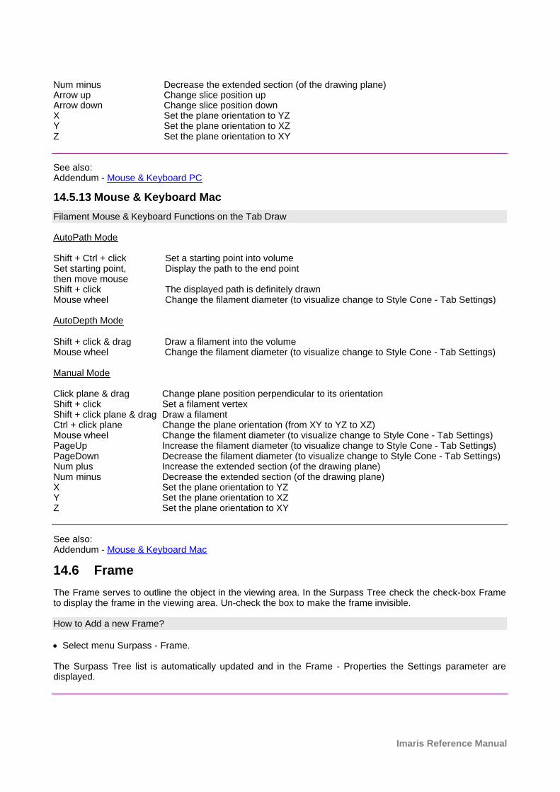
Imaris Reference Manual
Num minus Decrease the extended section (of the drawing plane)Arrow up Change slice position upArrow down Change slice position downX Set the plane orientation to YZY Set the plane orientation to XZZ Set the plane orientation to XY
See also:Addendum - Mouse & Keyboard PC
14.5.13 Mouse & Keyboard Mac
Filament Mouse & Keyboard Functions on the Tab Draw
AutoPath Mode
Shift + Ctrl + click Set a starting point into volumeSet starting point, then move mouse
Display the path to the end point
Shift + click The displayed path is definitely drawnMouse wheel Change the filament diameter (to visualize change to Style Cone - Tab Settings)
AutoDepth Mode
Shift + click & drag Draw a filament into the volumeMouse wheel Change the filament diameter (to visualize change to Style Cone - Tab Settings)
Manual Mode
Click plane & drag Change plane position perpendicular to its orientationShift + click Set a filament vertexShift + click plane & drag Draw a filamentCtrl + click plane Change the plane orientation (from XY to YZ to XZ)Mouse wheel Change the filament diameter (to visualize change to Style Cone - Tab Settings)PageUp Increase the filament diameter (to visualize change to Style Cone - Tab Settings)PageDown Decrease the filament diameter (to visualize change to Style Cone - Tab Settings)Num plus Increase the extended section (of the drawing plane)Num minus Decrease the extended section (of the drawing plane)X Set the plane orientation to YZY Set the plane orientation to XZZ Set the plane orientation to XY
See also:Addendum - Mouse & Keyboard Mac
14.6 Frame
The Frame serves to outline the object in the viewing area. In the Surpass Tree check the check-box Frameto display the frame in the viewing area. Un-check the box to make the frame invisible.
How to Add a new Frame?
· Select menu Surpass - Frame.
The Surpass Tree list is automatically updated and in the Frame - Properties the Settings parameter aredisplayed.
© Bitplane 2010
14.6.1 Tab Settings
Highlight Frame in the Surpass Tree and click on the tab Settings. The Frame Settings display in theproperties area.
Box and Time Settings
BoxCheck the parameter to display a box around the Frame.
Line WidthAdjust the box line width with the respective slider.Moving the slider to the left reduces the line width, movingit to the right increase line width.
ShadingCheck this parameter to display a shading. Use the slider to adjust the shade contrast.
ShadowThe entire Surpass scene can produce shadows on the three planes of the Frame object. Check this box todisplay the shadows. Use the Shading slider (see above) to adjust the contrast. The rendering is done inreal-time, and it requires a good performance of the graphics board (depending on the complexity of thescene).
Time ColorbarOnly available if you work with a time data set. Check this box and the Time Colorbar displays in the lowerleft corner of the viewing area.
Grid and Tickmarks Settings
GridCheck the box Grid to display a grid. Use the slider to adjust the grid width.Scale is shown using a grid behind the object. The frame moves to stay behind the object as it is rotated. Thedistance represented by each square in the grid, the scale bar, is shown in the bottom right corner of thescreen.
TickmarksCheck the box Tickmarks to display tickmarks on the edges of the frame.
Fix to Data SetCheck Fix to Data Set to fix the Frame to the same side when navigating the object.
SpacingSpecify the grid and tickmark spacing.
Labels Settings
Axis LabelsCheck the box Axis Labels to display the x, y, and z axes to clearly show the orientation of the object. If thisbox is checked the parameter Label Color and Label Font is available (see below).
Label ColorOnly available if the parameter Axis Labels (see above) is checked. Click on the icon to open the Color Editorwindow to change the color of the label on the coordinate axes.
Label FontOnly available if the parameter Axis Labels (see above) is checked. Click on the icon to open the Font Editorwindow to change the font to label the coordinate axes.
Imaris Reference Manual
14.6.2 Tab Color
Tab Color edit, manage and assign colors material to the Frame.
14.7 Group
Groups are folders in the Surpass Tree that contain other Surpass objects. They are visible in the objectsarea and allow you to create a treelike hierarchy of Surpass objects. When the first Surpass object iscreated, it is automatically placed in a Group called Surpass Scene. Additional Groups can be created inorder to sort objects of the scene.
How to Add a new Group?
· Select menu Surpass - Group.
The Surpass Tree list is automatically updated and in the Group - Properties the Settings parameter aredisplayed.
How to Add Items in a new Group?
· Click on an Item in the Surpass Tree list and drag it onto the Group object. Once released, the Item isadded to the Group.
Like all other objects, Groups have a visibility check-box. This box affects the visibility of all objects in theGroup.
See also:Surpass View - Overview - Surpass TreeSurpass View - Overview - Scene File Concept
14.7.1 Tab Settings
Number of ObjectsDisplays the number of objects in the Group.
Button Show AllIf you click this button the check-box(es) of the Item(s) in the Group are checked.
Button Hide AllIf you click this button the check-box(es) of the Item(s) in the Group are un-checked.
14.7.2 Tab Color- Base
Color Tab edit, manage and assign material colors of an Object.
RGB
The RGB color model is an additive color model in which Red, Green and Blue are combined together toreproduce an array of colors. The color values may be changed either by clicking on the color wheel to selecta color or by direct numeric entry for the Red, Blue or Green component (values range from 0 to 1).
Light reflection
Quality of the object material is further characterized by reflection properties. Diffusion- diffuses reflection of a matte, uneven material.Specular- defines reflection of highly reflective materials. The brighter a specular map is, the more shine is
© Bitplane 2010
applied to the object. Default setting has no specular intensity.Emission- light emitted from the material defines the self-illumination. Default setting emits no light.
Transparency
Transparency- defines the amount of light allowed to pass through an object. Click this tool to change thepercentage from 0% (complete opacity) to 100% (complete image transparency).
Palette
Palette- this option provides a system of preset colors organized into color schemes. In the Palette, colors are labeled and grouped together. The scrolling window contains the 14 colorcombination groups (Custom, artdeco, autumn, glass, metal, neon, rococo, santafe, sheen, silky, spring,summer, tropical, winter). Examples of colors in a selected group are displayed in the attached rectangulararea. If a custom color has been defined on the RGB tab, it can be added to the Custom palette with the Addto Palette button. After being added, these color choices are stored and can be used with other Imarisobjects.
14.7.3 Tab Statistics
The Statistics tab enables us to understand and compare different datasets through summarized statisticalvalues and graphical data presentations. To perform further analysis of large amounts of statistical data, usethe Group Level Statistic. The Statistics tab collects and displays the Group's statistical values, which arelists of the statistical value summaries of all created objects contained in the specified Group.For further analysis select the Export button and the statistic values of all objects are exported as a singlefile.
Several types of statistical tools enable convenient organization and analysis of heterogeneous statisticaldata. The Statistics View is configured as follows: a) Overall b) Detailed
In the statistical dataset the first column contains the name of the variable, followed by columns withcalculated statistical data. Corresponding statistical variable values are presented in rows.
Overall Tab
Output of the Overall statistics provides an overview of the image's single determining variables. Onlystatistics that are not measured on a per-object basis are displayed here.
Detailed Tab
A pull down list offers three types of Detailed statistical calculations: Specific ValuesAverage ValuesAll Values
Time Plots The values displayed are always for the current time point. Selecting a variable that changes over timecreates a plot of selected values as a time function. The statistical variable value is plotted on the verticalaxis and the time is plotted on the horizontal axis. The current time point is indicated with a black vertical line.Each time value is displayed as a point. Click inside the plot and move the time line. Moving the line changesthe time point. Altering the time point changes the variable value and the image.Multiple value selection, available by Ctrl+ click, will plot a superimposed second selected value over the firstone.
Interactive two-way SelectionA click on an individual row of the table highlights the corresponding object in the image. Similarly, by clickingon an element in the image (while the pointer is in Select mode) the corresponding row in table will behighlighted. A possibility of multiple selections is available by pressing Ctrl+click (Mac: Command+click).
Specific Values
Imaris Reference Manual
In the Specific Values, a second pull down list at the top of the window displays available specific statisticalvalues. Select the variable and a list of values will be displayed.
Average valuesThe Average table contains values determined on the basis of all values within a set of the selected variable.Columns are labeled as follows:Min (Minimum)- the smallest value within a set of values of the selected variable Max (Maximum)- the largest value within a set of values of the selected variable Mean – value of the sum of all values divided by number of values within a set Std Dev (Standard deviation)- a measure of the values distribution around the mean values Median- the middle value of the sorted set of variablesSum- the sum of all values within a variable setCount- number of values within a setUnit- variable unit Level/Distance
The black line on the time plot indicates where the mean value lies, the red indicates the median, the lightgray area shows the range between the min and max values and dark gray region labels the standarddeviation range with error bars.
Settings Button -Configure a List of visible statistics valuesClick on the button Settings and switch to the window Preferences
Search Button - Search by object IDType in the object ID in the data field. Click on the button Search. Highlights the object in the viewing areaHighlights the object on the Detailed TabDisplays of the values on the Selection Tab
Export Button - Export Statistics on Tab Display to FileOnly the statistics that are shown within the current tab will be exported.
Button Export - Export selected Data for plottingExports the selected statistical value for plotting. The selected value has to be time dependent.With a click on the button Export the Export Statistics window opens. Select the file type (CommaSeparated Values *.csv, Excel file *.xls, or Excel XML *.xlm). If you select MS Excel as file type, the programstarts automatically.
Export Button - Export All Statistics to FileAll of the statistics (that are enabled in the statistics settings) will be exported.With a click on the button Export the window Export Statistics opens. Select the file type (Comma SeparatedValues *.csv, Excel file *.xls, or Excel XML *.xlm). If you select MS Excel as file type, the program startsautomatically and the sheets show up one after another (this will take several seconds).
14.8 Light Source
A Light Source serves to illuminate objects in the viewing area. A light source node serves as the locationand orientation of a light source.
How to Add a new Light Source?
· Select menu Surpass - Light Source.
The Surpass Tree list is automatically updated and in the Light Source - Properties the Settings parameterare displayed. Multiple light sources can be added in the Surpass Tree.
Move Light Source
To change the Light Source position and direction, choose the pointer mode Select and drag the cone or line.
Light Intensity
© Bitplane 2010
Click on the cylinder above the cone and move it closer or further away from the object to change the lightintensity.
See also:Surpass View - Overview - Surpass Tree Surpass View - Overview - Camera Toolbar - Pointer (Mode Select)
14.8.1 Tab Settings
Fix to Data SetCheck the box to fix the Light Source to the same side when navigating the object. When the box isun-checked, the light source is fixed to a particular position in space and remains in place when the objectmoves or rotates.
14.8.2 Tab Color
Color Tab edit, manage and assign material colors of an Object.
RGB
The RGB color model is an additive color model in which Red, Green and Blue are combined together toreproduce an array of colors. The color values may be changed either by clicking on the color wheel to selecta color or by direct numeric entry for the Red, Blue or Green component (values range from 0 to 1).
Palette
Palette- this option provides a system of preset colors organized into color schemes. In the Palette, colors are labeled and grouped together. The scrolling window contains the 14 colorcombination groups (Custom, artdeco, autumn, glass, metal, neon, rococo, santafe, sheen, silky, spring,summer, tropical, winter). Examples of colors in a selected group are displayed in the attached rectangulararea. If a custom color has been defined on the RGB tab, it can be added to the Custom palette with the Addto Palette button. After being added, these color choices are stored and can be used with other Imarisobjects.
14.8.3 Mouse & Keyboard PC
Light Source Mouse & Keyboard Functions
Left-click cone (or line) & drag Change directionLeft-click cylinder & drag Change intensity
See also:Addendum - Mouse & Keyboard PC
14.8.4 Mouse & Keyboard Mac
Light Source Mouse & Keyboard Functions
Click cone (or line) & drag Change directionClick cylinder & drag Change intensity
See also:Addendum - Mouse & Keyboard Mac
Imaris Reference Manual
14.9 Measurement Point
How to Add a new Measurement Point?
· Select menu Surpass - Measurement Point.
The Surpass Tree list is automatically updated and in the Measurement Point - Properties the Editparameters are displayed.
14.9.1 Tab Settings
Point Shape
TetrahedronCubeSphereHere you can choose from three different shapes for the Measurement Points (tetrahedron, cube, or sphere).
FilledCheck the box and the point shape is solid.
Point Diameter
Here you can define the Measurement Point diameter.
Point Labels
NameCheck the check-box to display the name of a Measurement Point in the viewing area.
IntensityCheck the check-box to display the intensity of a Measurement Point in the viewing area. The intensity of thechannel is displayed in brackets.
Line Mode
Pairs (AB, CD, ...)Any two consecutive points are connected by a line.
Polygon (ABCD ...)All points in the Group are connected consecutively (P1-P2-P3-P4, etc.).
Line Width
Here you define the line width.
Line Labels
DistanceThe measured distance between two points is displayed next to the line connecting the two MeasurementPoints. Check the check-box to display the distances in the viewing area.
VelocityOnly accessible if you have a time data set. Check the box to display the speediness between twoMeasurement Points.
Tip: If you do not have the module ImarisTrack you can easily use the velocity function to track single objectsover several time points and measure the velocity.

© Bitplane 2010
Button ColorButton Font Label Color and FontTo change the color or font of the label (display of the line length) click on the respective icon.
Tip: You can find the parameters to change the color of the Measurement Points and connecting lines on thetab Colors.
Visible for all Time PointsOnly accessible if you have a time data set. Check the box to display the inserted Measurement Points, lines,and annotations at all time points.
See also:Surpass View - Measurement Point - Tab Color
14.9.2 Tab Edit
Autodepth Position
In the mouse pointer mode Select:Shift-click with the left mouse button to add a new point. Left-click to select an existing point. Shift-left-click to reposition a selected point.
Intersect with
The first two parameters are relevant if you want to insert Measurement Points in a volume rendered dataset. For the rest the last parameter is crucial.
all visible ChannelIn the Display Adjustments you decide, whether a channel is visible or not in the viewing area. Select thisparameter and all visible channel are relevant for the placement of the Measurement Points.
specific ChannelsIn the Display Adjustments you decide, whether a channel is visible or not in the viewing area. Select thisoption and choose the channel directly from the drop down list. The selected channel is relevant for the placement of the Measurement Points.
solid ObjectsCheck this box and the Measurement Points are placed on the surface of an object. Un-check the box andyou can also place Measurement Points in an object.
Button Delete All PointsClick on this button to delete all Measurement Points. Alternatively click on the Delete-key on the keyboard.
Selected Point
Click to select an existing point. If no point is selected the following parameters are grayed. Re-click on aselected point to un-select the point.
Button DeleteClick on this button to delete the selected Measurement Point.
NameText field to edit the Measurement Point name.
PositionXYZTData field of the x-, y-, z- and t-coordinates.
Imaris Reference Manual
See also:Menu Edit - Show Display AdjustmentSurpass View - Overview - Camera Toolbar (Pointer Select)
14.9.3 Tab Intensity
Imaris reads out the intensity profile of each voxel against the distance. Here you select the channels thatshould be displayed in the histogram and you choose the desired connecting lines between the MeasurementPoints.
Histogram
The histogram displays the intensity profile along the lines. The labeled lines represent the MeasurementPoints. The x-axis represents the length of the profile. On the left hand side of the histogram you find thedisplay of the channel(s) intensity range. The channel selection is located below the histogram. Here you canswitch channels in the intensity profile on or off. Below the channel selection you find the profile selection. Inthe drop-down list select the desired line and the histogram updates accordingly.
Button SnapshotClick on this button to do a Snapshot of the histogram. The window Save Snapshot as... opens.
See also:Menu File - Save as... Snapshot
14.9.4 Tab Statistics
Measurement Point statistics are automatically computed. For the statistical values please refer to thechapter Menu Edit - Preferences... - Statistics - Measurement Points. The Statistics tab collects and displaysthe image's statistical values in Imaris. The Statistics tab enables us to understand and compare differentdatasets through summarized statistical values and graphical data presentations. Several types of statistical tools enable convenient organization and analysis of heterogeneous statisticaldata. The Statistics View is configured as follows: a) Overall b) Detailedc) SelectionIn the statistical dataset the first column contains the name of the variable, followed by columns withcalculated statistical data. Corresponding statistical variable values are presented in rows. To sort the columns click on the arrow in column heading. Click again to reverse the sort.
Overall Tab
Output of the Overall statistics provides an overview of the image's single determining variables. Onlystatistics that are not measured on a per-object basis are displayed here.
Category
A Category identifies, gathers and summaries a set of statistical values calculations of a particular ObjectType. Statistical values associated with one object type are grouped in one category. Each category has anassociated button with graphical indications of Category type.In Imaris there are following Filter Categories: Surface , Surface Tracks , Spots , Spots Tracks ,
Dendrites , Dendrites Tracks , Filament , Filament Tracks , Spines , Spine Tracks , Point ,
Point Tracks , Cell , Cell Tracks , Nucleus , Nucleus Tracks , Vesicle and Vesicles Tracks
. These buttons allow you to choose the Category and determines the list of displayed statistical values.Clicking the button selects the corresponding category (the category button turns black) and the list ofstatistical values is displayed according to the selection.To remove the category from the list, re-click on the Category button. Re-clicking on the category button
© Bitplane 2010
deselects Category and removes the selected statistical values from the list (turns the category button into alight gray color).
The exclamation mark sign indicates that the listed statistical parameter does not contain any value.
Detailed Tab
A pull down list offers three types of Detailed statistical calculations: Specific ValuesAverage ValuesAll Values
Time Plots The values displayed are always for the current time point. Selecting a variable that changes over timecreates a plot of selected values as a time function. The statistical variable value is plotted on the verticalaxis and the time is plotted on the horizontal axis. The current time point is indicated with a black vertical line.Each time value is displayed as a point. Click inside the plot and move the time line. Moving the line changesthe time point. Altering the time point changes the variable value and the image.Multiple value selection, available by Ctrl+ click, will plot a superimposed second selected value over the firstone.
Interactive two-way SelectionA click on an individual row of the table highlights the corresponding object in the image. Similarly, by clickingon an element in the image (while the pointer is in Select mode) the corresponding row in table will behighlighted. A possibility of multiple selections is available by pressing Ctrl+click (Mac: Command+click).
Specific Values In the Specific Values, a second pull down list at the top of the window displays available specific statisticalvalues. Select the variable and a list of values will be displayed.
Average valuesThe Average table contains values determined on the basis of all values within a set of the selected variable.Columns are labeled as follows:Min (Minimum)- the smallest value within a set of values of the selected variable Max (Maximum)- the largest value within a set of values of the selected variable Mean – value of the sum of all values divided by number of values within a set Std Dev (Standard deviation)- a measure of the values distribution around the mean values Median- the middle value of the sorted set of variablesSum- the sum of all values within a variable setCount- number of values within a setUnit- variable unit Level/Distance
The black line on the time plot indicates where the mean value lies, the red indicates the median, the lightgray area shows the range between the min and max values and dark gray region labels the standarddeviation range with error bars.
All valuesIf the option All values is selected for the detailed tab, all values will be displayed. Even thought this option isalways readily available, it is discouraged to use it in order to avoid data clutter.
Selection Tab
Statistical tables for a selected object will be displayed. Change to the pointer mode Select and click on animage elementthat has been detected/segmented. A possibility of multiple selections is available by Ctrl+click(Mac: Command-click).A pull down list offers three types of statistical calculations from a Selection:Specific ValuesAverage ValuesAll Values
Imaris Reference Manual
Time Plots The values displayed are always for the current time point. Selecting a variable that changes over timecreates a plot of selected values as a time function. The statistical variable value is plotted on the verticalaxis and the time is plotted on the horizontal axis. The current time point is indicated with a black vertical line.Each time value is displayed as a point. Click inside the plot and move the time line. Moving the line changesthe time point. Altering the time point changes the variable value and the image.Multiple value selection, available by Ctrl+ click, will plot a superimposed second selected value over the firstone.
Interactive two-way SelectionA click on an individual row of the table highlights the corresponding object in the image. Similarly, by clickingon an element in the image (while the pointer is in Select mode) the corresponding row in table will behighlighted. A possibility of multiple selections is available by pressing Ctrl+click (Mac: Command+click).
Specific valuesIn the Specific Values, a second pull down list at the top of the window displays available specific statisticalvalues. Select the variable and a list of values will be displayed.
Average valuesThe Average table contains values determined on the basis of all the values within a set of the selectedvariables for the selected image element(s). For further explanation see Average values Detailed statistics.This choice only makes sense in the context of the Selection Tab if you have selected more than oneelement from the image.
The black line on the time plot indicates where the mean value lies, the red indicates the median, the lightgray area shows the range between the min and max values and dark gray region labels the standarddeviation range with error bars.
Buttons at the bottom of the Statistics tab
Button Settings -Configure a List of visible statistics values. Click on the button Settings and you switch to the window Preferences - Statistics - Measurement Points.
Button Search - Search by object ID.Type in the object ID in the data field. Click on the button Search. · Highlights the object in the viewing area· Highlights the object on the Detailed Tab· Displays of the values on the Selection Tab
Button Measurement Points - Duplicate Selection to new Measurement Points.Click on this button and all selected elements are copied to a new object. The new Measurement Pointsappears in the Surpass Tree, and the old one is hidden, but still available.
Button Export - Export Statistics on Tab Display to File. Only the statistics that are shown within the current tab will be exported.
Button Export - Export selected Data for plottingExports the selected statistical value for plotting. The selected value has to be time dependent.With a click on the button Export the Export Statistics window opens. Select the file type (CommaSeparated Values *.csv, Excel file *.xls, or Excel XML *.xlm). If you select MS Excel as file type, the programstarts automatically.
Button Export - Export All Statistics to File. All of the statistics (that are enabled in the statistics settings) will be exported.With a click on the button Export the Export Statistics window opens. Select the file type (CommaSeparated Values *.csv, Excel file *.xls, or Excel XML *.xlm). If you select MS Excel as file type, the programstarts automatically and the sheets show up one after another (this will take several seconds).

© Bitplane 2010
Buttons Overview
PC: Mac: Select Spot Left-click Click Select multiple Spots Ctrl + left-click Command + click
See also:Menu Edit - Preferences... - Statistics - Measurement Points
14.9.5 Tab Color
Color Tab edit, manage and assign material colors of an Object.
RGB
The RGB color model is an additive color model in which Red, Green and Blue are combined together toreproduce an array of colors. The color values may be changed either by clicking on the color wheel to selecta color or by direct numeric entry for the Red, Blue or Green component (values range from 0 to 1).
Light reflection
Quality of the object material is further characterized by reflection properties. Diffusion- diffuses reflection of a matte, uneven material.Specular- defines reflection of highly reflective materials. The brighter a specular map is, the more shine isapplied to the object. Default setting has no specular intensity.Emission- light emitted from the material defines the self-illumination. Default setting emits no light.
Transparency
Transparency- defines the amount of light allowed to pass through an object. Click this tool to change thepercentage from 0% (complete opacity) to 100% (complete image transparency).
Palette
Palette- this option provides a system of preset colors organized into color schemes. In the Palette, colors are labeled and grouped together. The scrolling window contains the 14 colorcombination groups (Custom, artdeco, autumn, glass, metal, neon, rococo, santafe, sheen, silky, spring,summer, tropical, winter). Examples of colors in a selected group are displayed in the attached rectangulararea. If a custom color has been defined on the RGB tab, it can be added to the Custom palette with the Addto Palette button. After being added, these color choices are stored and can be used with other Imarisobjects.
14.9.6 Mouse & Keyboard PC
Measurement Point Mouse & Keyboard Functions on the Tab Edit
Shift + left-click Add a new measurement pointShift + left-click Reposition selected measurement pointLeft-click on existing point Select measurement pointMouse wheel in Add mode Turn wheel up: Increase size of next measurement point
Turn wheel down: Decrease size of next measurement point
Depending on the depth of the structure where you want to put the next Measurement Point, the size of theshape around the mouse pointer changes accordingly. This helps a lot in handling 3D data sets.
See also:Menu Edit - Preferences ... - 3D Cursor (adjust 3D Cursor Shape) Addendum - Mouse & Keyboard PC
Imaris Reference Manual
14.9.7 Mouse & Keyboard Mac
Measurement Point Mouse & Keyboard Functions on the Tab Edit
Shift + click Add a new measurement pointShift + click Reposition selected measurement pointClick on existing point Select measurement point
Depending on the depth of the structure where you want to put the next Measurement Point, the size ofshape around the mouse pointer changes accordingly. This helps a lot in handling 3D data sets.
See also:Menu Edit - Preferences ... - 3D Cursor (adjust 3D Cursor Shape)Addendum - Mouse & Keyboard Mac
14.10 Oblique Slicer
The Oblique Slicer represents a plane that can be freely moved and rotated within the data set and allowsyou to look inside any object. The Oblique Slicer consists of a colored frame with a white double rod in themiddle.
How to Add a new Ortho Slicer?
· Select menu Surpass - Oblique Slicer.
The Surpass Tree list is automatically updated and in the Oblique Slicer - Properties the Settings parameterare displayed. The Oblique Slicer is displayed in the viewing area (depending on the default parameter on thetab Settings).
Change Position of the Oblique Slicer
You can change the position of the Oblique Slicer. Choose the pointer mode Select, highlight the ObliqueSlicer in the viewing area and click on the bigger diameter rod. It will turn colored as it is selected, move it toset the Oblique Slicer to the required position.
Rotate Oblique Slicer around Axes
The Oblique Slicer can be rotated around the x-, y-, and the z-axes. In Select mode click the smallerdiameter rod. It will be highlighted as it is selected. To rotate the Oblique Slicer, move the smaller rod.
See also:Surpass View - Overview - Camera Toolbar - Pointer (Mode Select)Surpass View - Ortho Slicer - Tab Settings
14.10.1 Tab Settings
Orientation
Button YZ PlaneButton XZ PlaneButton XY PlaneChange the Slicer direction, if required, by selecting the adequate plane.
Position
Button RecenterClick on this button to re-center the Slicer.
Extended Section
© Bitplane 2010
The section is a single cut through the data set, the highlighted lines indicate the frame around the activeslice. In the data field you can adjust the distance between the two lines.
Show FrameCheck the box to display a colored frame around the Slicer.
Camera
Button Orthogonal ViewThe camera is set to a position which is perpendicular to the Slicer.
14.10.2 Mouse & Keyboard PC
Oblique Slicer Mouse & Keyboard Functions
Left-click on the bigger diameter rod & drag Move plane to desired positionLeft-click on the smaller diameter rod & drag Rotate plane to desired position
See also:Addendum - Mouse & Keyboard PC
14.10.3 Mouse & Keyboard Mac
Oblique Slicer Mouse & Keyboard Functions
Click on the bigger diameter rod & drag Move plane to desired positionClick on the smaller diameter rod &drag
Rotate plane to desired position
See also:Addendum - Mouse & Keyboard Mac
14.11 Ortho Slicer
Ortho Slicer represent an orthogonal plane (orthogonal to the coordinate axis of the data set) that can bemoved within the data set. When adding slices, Surpass suggests per default the directions z, x, and y assequence for the first three and all subsequent slices.
How to Add a new Ortho Slicer?
· Select menu Surpass - Ortho Slicer.
The Surpass Tree list is automatically updated and in the Ortho Slicer - Properties the Settings parameter aredisplayed. The first Slice is displayed in the viewing area (depending on the default parameter on the tabSettings).
See also:Surpass View - Ortho Slicer - Tab Settings
14.11.1 Tab Settings
Slice Orientation
YZ PlaneXZ PlaneXY PlaneThe check XY, XZ and YZ plane, to select the visibility of the corresponding slice.
Imaris Reference Manual
Extended Section
The section is a single cut through the data set, the colored lines indicate the frame around the active slice.In the data field you can adjust the distance between the two lines.
Show FrameCheck the box to display a colored frame around the active slice.
Slice Position
SliderChoose the relative position of the Slice in the data set by means of the slider or a direct entry of the sliceposition given as the offset distance from the data set origin (equals the absolute coordinates).
14.11.2 Mouse & Keyboard PC
Ortho Slicer Mouse & Keyboard Functions
Left-click plane & drag Change slice positionRight-click plane Change slice orientationNum plus Increase the extended sectionNum minus Decrease the extended sectionArrow up Change slice position upArrow down Change slice position down
See also:Addendum - Mouse & Keyboard PC
14.11.3 Mouse & Keyboard Mac
Ortho Slicer Mouse & Keyboard Functions
Click plane & drag Change slice positionCtrl + click plane Change slice orientationNum plus Increase the extended sectionNum minus Decrease the extended section
See also:Addendum - Mouse & Keyboard Mac
14.12 Spots
The Spots object is available to model point-like structures in the data. It provides a procedure toautomatically detect point-like structures, an editor to manually correct detection errors, a viewer to visualizethe point-like structures as spheres, and statistics output.
How to Add new Spots?
· Select menu Surpass - Spots.
The Surpass Tree list is automatically updated and the first window of the Creation Wizard displays in theSpots - Properties.
See also:Suprass View - Spots - Creation Wizard
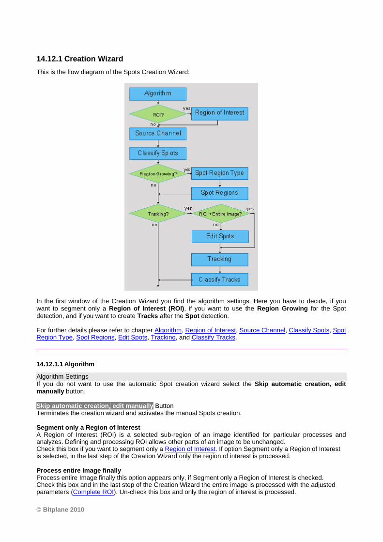
© Bitplane 2010
14.12.1 Creation Wizard
This is the flow diagram of the Spots Creation Wizard:
In the first window of the Creation Wizard you find the algorithm settings. Here you have to decide, if youwant to segment only a Region of Interest (ROI), if you want to use the Region Growing for the Spotdetection, and if you want to create Tracks after the Spot detection.
For further details please refer to chapter Algorithm, Region of Interest, Source Channel, Classify Spots, SpotRegion Type, Spot Regions, Edit Spots, Tracking, and Classify Tracks.
14.12.1.1 Algorithm
Algorithm SettingsIf you do not want to use the automatic Spot creation wizard select the Skip automatic creation, editmanually button.
Skip automatic creation, edit manually Button Terminates the creation wizard and activates the manual Spots creation.
Segment only a Region of InterestA Region of Interest (ROI) is a selected sub-region of an image identified for particular processes andanalyzes. Defining and processing ROI allows other parts of an image to be unchanged.Check this box if you want to segment only a Region of Interest. If option Segment only a Region of Interestis selected, in the last step of the Creation Wizard only the region of interest is processed.
Process entire Image finallyProcess entire Image finally this option appears only, if Segment only a Region of Interest is checked.Check this box and in the last step of the Creation Wizard the entire image is processed with the adjustedparameters (Complete ROI). Un-check this box and only the region of interest is processed.
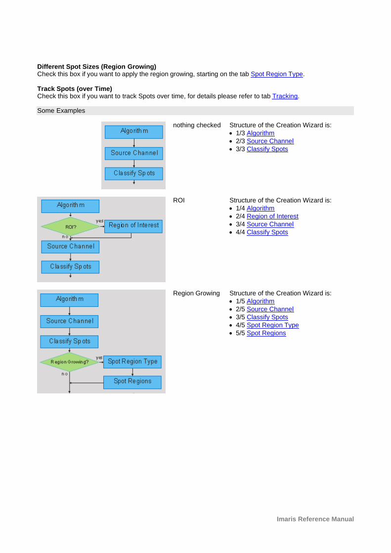
Imaris Reference Manual
Different Spot Sizes (Region Growing)Check this box if you want to apply the region growing, starting on the tab Spot Region Type.
Track Spots (over Time)Check this box if you want to track Spots over time, for details please refer to tab Tracking.
Some Examples
nothing checked Structure of the Creation Wizard is: · 1/3 Algorithm· 2/3 Source Channel· 3/3 Classify Spots
ROI Structure of the Creation Wizard is:· 1/4 Algorithm· 2/4 Region of Interest· 3/4 Source Channel· 4/4 Classify Spots
Region Growing Structure of the Creation Wizard is:· 1/5 Algorithm· 2/5 Source Channel· 3/5 Classify Spots· 4/5 Spot Region Type· 5/5 Spot Regions
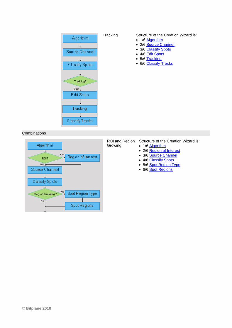
© Bitplane 2010
Tracking Structure of the Creation Wizard is:· 1/6 Algorithm· 2/6 Source Channel· 3/6 Classify Spots· 4/6 Edit Spots· 5/6 Tracking· 6/6 Classify Tracks
Combinations
ROI and RegionGrowing
Structure of the Creation Wizard is: · 1/6 Algorithm· 2/6 Region of Interest· 3/6 Source Channel· 4/6 Classify Spots· 5/6 Spot Region Type· 6/6 Spot Regions
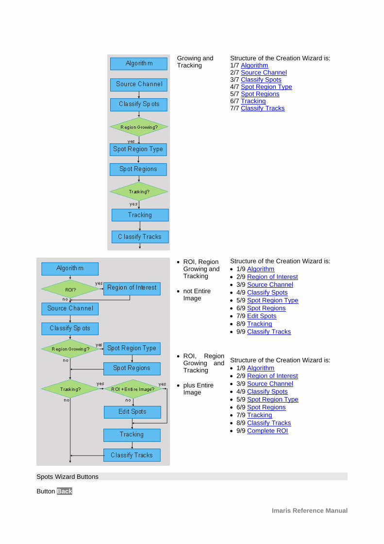
Imaris Reference Manual
Growing andTracking
Structure of the Creation Wizard is: 1/7 Algorithm2/7 Source Channel3/7 Classify Spots4/7 Spot Region Type5/7 Spot Regions6/7 Tracking7/7 Classify Tracks
· ROI, RegionGrowing andTracking
· not EntireImage
· ROI, RegionGrowing andTracking
· plus EntireImage
Structure of the Creation Wizard is:· 1/9 Algorithm· 2/9 Region of Interest· 3/9 Source Channel· 4/9 Classify Spots· 5/9 Spot Region Type· 6/9 Spot Regions· 7/9 Edit Spots· 8/9 Tracking· 9/9 Classify Tracks
Structure of the Creation Wizard is:· 1/9 Algorithm· 2/9 Region of Interest· 3/9 Source Channel· 4/9 Classify Spots· 5/9 Spot Region Type· 6/9 Spot Regions· 7/9 Tracking· 8/9 Classify Tracks· 9/9 Complete ROI
Spots Wizard Buttons
Button Back
© Bitplane 2010
This button is grayed in the first window of the Creation Wizard.
Button NextPress Next to proceed with the next window of the Creation Wizard.
Button FinishClick on Finish to calculate the desired Spots and display the Spots in the viewing area.
Button CancelIf you do not want to create Spots click on Cancel.
14.12.1.2 Region of Interest
Region of Interest 1
Here you define the region of interest (ROI). Parameters such as width, height and location of the ROI areused to directly specify the area to work on.
X, Y, Z, TimeMin, Max, SizeMinimum, maximum and Size of ROI coordinate values, can be specified either by entering the value in thevalue fields or changing the values by clicking on up-and down arrows at the right hand side of the valuefields.Alternatively the location and size of the ROI can be adjusted directly in the viewing area. Size of the ROI:1. Click on the ROI preview rectangle arrows (change to the pointer mode Select) 2. Drag the arrows to define new coordinates for X ,Y and Z. Location of the ROI: 1.Click inside the ROI preview rectangle 2. Drag the entire rectangle (with mouse button held) to the chosen image location. The numbers in the value fields are updated automatically.
Memory Usage:Display of the memory usage for the image size within the ROI.
Regions of Interest
To select a particular ROI, left-click on its name in the list and the selected ROI will be highlighted within animage and its properties can be adjusted.
Button AddClick on this button and a new region of interest appears in the list. To adjust this ROI you have to select theROI with a left mouse click.
Button DeleteSelect a ROI in the list with a left mouse click and click on this button to delete the ROI.
Total Memory Usage:Display of the memory usage for the image size within the ROI.
Spots Wizard Buttons
Button BackWith Back you return to the previous window of the Creation Wizard.
Button NextPress Next to proceed with the next window of the Creation Wizard.
Button FinishClick on Finish to calculate the desired Spots and display the Spots in the viewing area.
Imaris Reference Manual
Button CancelIf you do not want to create Spots automatically click on Cancel.
See also:Surpass View - Overview - Camera Toolbar (change to pointer mode Select)
14.12.1.3 Source Channel
Source Channel
Select the respective source channel, from which the Spots are to be computed.
Spot Detection
Estimated DiameterObjects with size smaller than specified Estimated Diameter are not detected. This is also the diameter ofthe inserted Spots.
Background Object SubtractionIf checked, the background will be removed prior to spot detection. Technically background subtractionsmoothes the image. The intensity is the one of a Gaussian filtered channel (Gaussian filtered by 3/4) minusthe intensity of the original channel Gaussian filtered by 8/9 of sphere radius.
Spots Wizard Buttons
Button BackWith Back you return to the previous window of the Creation Wizard.
Button NextPress Next to proceed with the next window of the Creation Wizard.
Button FinishClick on Finish to calculate the desired Spots and display the Spots in the viewing area.
Button CancelIf you do not want to create Spots click on Cancel.
14.12.1.4 Classify Spots
The Spots filtering is incorporated into the creation process.
A filtering allows the removal of objects that would interfere with interpretation of results.
Quality: The 'Quality' is the intensity at the center of the spot in the channel the spot was detected.
If 'Background Subtraction' was not checked this is the intensity of the channel Gaussian filtered by 3/4 ofspot radius. If 'Background Subtraction' was active the intensity is the one of a Gaussian filtered channel from aboveminus the intensity of the original channel Gaussian filtered by 8/9 of spot radius.
The Filter Type and its values define the section of interest, from this selection, which includes or excludesobjects based on a range of criteria. Select the filter type by selecting a variable from the drop-down list, andthen define the filter values, which will then limit the selection just to those objects that meet the set upcriteria. In Imaris you can choose two filter values, a Lower and a Higher filter value. The two filter values separate the data into three regions: above the higher value, below the lower value, andthe region in between. Objects with the relevant properties below the Lower filter value and objects with theproperties exceeding the Higher filter value will be excluded, and only those objects with qualities inside the
© Bitplane 2010
defined interval will be considered.
Please note if the value of the Lower filter value is set to be higher than that of the Higher filter value, theselected objects will be outside the defined interval. Only those objects meeting all the filter criteria areinteractively shown and instantly highlighted in the viewing area.
By using multiple filter types, more than one criterion can be specified for the data analyses.
Filters
Add ButtonTo add a new filter, click on the button Add and choose one of the Filter Types from the drop-down menu.Select the filtering type to be used in order to classify objects and specify the measurement of the criteria tobe used. The new filter appears in the list.
Delete ButtonSelect a filter in the list with a left mouse click and click on this button to delete the filter.
Filter Type
Select in the drop down list the filter you want to apply.
Filter category
A Category identifies, gathers and summaries a set of statistical values calculations of a particular ObjectType. Statistical values associated with one object type are grouped in one category. Each category has anassociated button with graphical indications of Category type.In Imaris there are following Filter Categories: Surface , Surface Tracks , Spots , Spots Tracks ,
Dendrites , Dendrites Tracks , Filament , Filament Tracks , Spines , Spine Tracks , Point ,
Point Tracks , Cell , Cell Tracks , Nucleus , Nucleus Tracks , Vesicle and Vesicles Tracks
. These buttons allow you to choose the Category and determines the list of displayed statistical values.Clicking the button selects the corresponding category (the category button turns black) and the list ofstatistical values is displayed according to the selection.To remove the category from the list, re-click on the Category button. Re-clicking on the category buttonde-selects Category and removes the selected statistical values from the list (turns the category button into alight gray color).
The exclamation mark sign indicates that the listed statistical parameter does not contain any value.
Lower and Upper Threshold
Activating/deactivating the Lower or Upper threshold option is done by clicking on the or button. The
Red button indicates that the threshold option is currently inactive, while the green button indicates anactive threshold.In order to activate the threshold option, click on the red button. To deactivate the threshold, click on thegreen circle again.
Automatic/Manual A/M buttonThe Automatic/Manual A/M button provides a single interaction point for the direct choice of the thresholdvalue adjustment.
When the lower/upper threshold values are not activated (the red button ) the corresponding A/M button islight gray indicating that threshold adjustment is unavailable. When the lower/upper threshold option is
activated (the green button ), the corresponding A/M button turns black.
After the first threshold activation, as a default, an Automatic threshold value is activated . Clicking onthe Automatic/Manual button allows you to switch between an Automatic and a Manual threshold adjustmentmode. The A/M button provides a visual feedback as an indication of the selected threshold adjustment
mode. Clicking on the A/M button changes the appearance of the A/M button form indicating an
Imaris Reference Manual
activated Automatic threshold to indicating a Manual threshold. Clicking on the histogram automatically activates a Manual threshold adjustment.
Lower Threshold
AutomaticThe initial threshold value is automatically computed.
ManualDefine the threshold by clicking into the histogram or by entering the value directly in the data field. Eithertype in the value or click into the histogram to move the colored line and a reduced/enlarged set of objects isvisualized.
Higher Threshold
AutomaticThe initial threshold value is automatically computed.
ManualDefine the threshold by clicking into the histogram or by entering the value directly in the data field. Eithertype in the value or click into the histogram to move the colored line and a reduced/enlarged set of objects isvisualized.
Histogram
In the histogram the regions above and below the threshold values are displayed in white, while region withinthreshold is displayed in yellow. To change the automatically set threshold values, select the option Manual.By clicking into the histogram you move the colored line and the reduced/enlarged set of objects. To changethe Lower threshold value left click on the histogram and drag the yellow line.To change the Higher threshold value right click on the histogram and move the line. Move the line to theright to increase the threshold, while to decrease the threshold move the line to the left. These changes areinstantly visible in the viewing area.The numerical range of the statistics value (e.g. Quality), the number and percentage of objects selected(e.g. Surfaces) is displayed at the bottom of the threshold histogram.
Spots Wizard Buttons
Button BackWith Back you return to the previous window of the Creation Wizard. Button NextPress Next to proceed with the next window of the Creation Wizard.
Button FinishClick on Finish to calculate the desired Spots and display the Spots in the viewing area.
Button CancelIf you do not want to create Spots click on Cancel.
14.12.1.5 Spot Region Type
This tab only appears, if Different Spot Sizes (Region Growing) is checked (Algorithm Settings).
The region method for segmentation in Imaris starts with defined seed points. You use Spots as seed pointsfor the region growing that is performed in the next steps. During the region growing process around eachseed point the region grows until a border stops the growing.
Spot Regions from
Absolute Intensity
© Bitplane 2010
Local ContrastYou can set the border using the Absolute Intensity or the Local Contrast as criteria. In both cases as nextstep the selected channel is displayed in the viewing area.
Spots Wizard Buttons
Button BackWith Back you return to the previous window of the Creation Wizard.
Button NextPress Next to proceed with the next window of the Creation Wizard.
Button FinishClick on Finish to calculate the desired Spots and display the Spots in the viewing area.
Button CancelIf you do not want to create Spots click on Cancel.
14.12.1.6 Spot Region
This tab only appears, if Different Spot Sizes (Region Growing) is checked (Algorithm Settings).
Spot Regions
The working channel is visualized in the viewing area, the histogram is displayed in the properties area.Regions above the threshold are displayed in white, regions below threshold are displayed in black.Depending on the previously selected detection method (Absolute Intensity or Local Contrast) refer toAbsolute Intensity or Local Contrast.
Compact Lower and Upper Threshold
Activating/deactivating the Lower or Upper threshold option is done by clicking on the or button. The
Red button indicates that the threshold option is currently inactive, while the green button indicates anactive threshold.In order to activate the threshold option, click on the red button. To deactivate the threshold, click on thegreen circle again.
Automatic/Manual A/M buttonThe Automatic/Manual A/M button provides a single interaction point for the direct choice of the thresholdvalue adjustment.
When the lower/upper threshold values are not activated (the red button ) the corresponding A/M button islight gray indicating that threshold adjustment is unavailable. When the lower/upper threshold option is
activated (the green button ), the corresponding A/M button turns black.
After the first threshold activation, as a default, an Automatic threshold value is activated . Clicking onthe Automatic/Manual button allows you to switch between an Automatic and a Manual threshold adjustmentmode. The A/M button provides a visual feedback as an indication of the selected threshold adjustment
mode. Clicking on the A/M button changes the appearance of the A/M button form indicating an
activated Automatic threshold to indicating a Manual threshold. Clicking on the histogram automatically activates a Manual threshold adjustment.
Absolute Intensity
AutomaticIn the working channel a copy of the intensity histogram of the source channel is displayed. Regions abovethe threshold are displayed in white. Now you adjust the threshold of the working channel. Edit the data fieldor adjust the threshold manually using the mouse (click & drag the line in the histogram). In the next step theregions will grow until they fill the white regions and reach the border.
Imaris Reference Manual
Local Contrast
AutomaticIn the selected channel the regions with a local contrast brighter than the background are displayed in white.Now you adjust the threshold value of the local contrast channel. Edit the data field or adjust the thresholdmanually using the mouse (click & drag the line in the histogram). In the next step the regions will grow untilthey fill the white regions and reach the border.
Diameter from
Region VolumeThe Spot(s) radius is calculated from the region volume (the region volume and the Spot volume are equal).
Region BorderThe radius of the calculated Spot(s) is the smallest distance from each Spot center to the region border.
Create Color Coded Region ChannelAdditional to the Spots the Region Channel is displayed. Each region has a different color.
Preview
Here you select the preview settings.
Ortho SlicerCheck this box if you want to see the ortho slicer in the preview.
Volume RenderingCheck this box if you want to see a volume rendering in the preview.
Slicer Plane XY, XZ, YZIf you check the box Ortho Slicer (see above) these radio buttons are available to select the slicer plane.
Show SpotsCheck this box to see the spots in the preview.
Button Change Regions ColorClick on this button to change the regions color.
Spots Wizard Buttons
Button BackWith Back you return to the previous window of the Creation Wizard.
Button NextPress Next to proceed with the next window of the Creation Wizard.
Button FinishClick on Finish to calculate the desired Spots and display the Spots in the viewing area.
Button CancelIf you do not want to create Spots click on Cancel.
14.12.1.7 Edit Spots
Tip: In the Surpass view be sure that the mouse is in the pointer mode Navigate. Switch between the twopointer modes Select/Navigate with the ESC-key.
Autodepth Draw
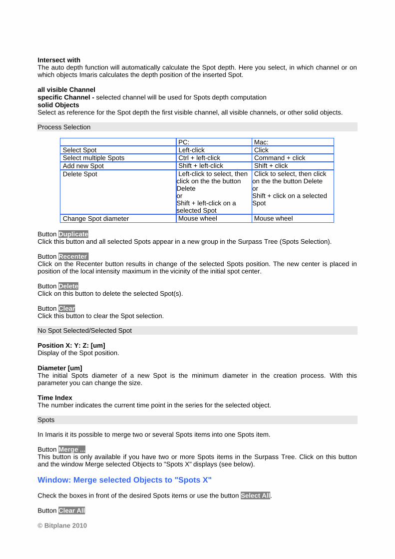
© Bitplane 2010
Intersect withThe auto depth function will automatically calculate the Spot depth. Here you select, in which channel or onwhich objects Imaris calculates the depth position of the inserted Spot.
all visible Channelspecific Channel - selected channel will be used for Spots depth computationsolid ObjectsSelect as reference for the Spot depth the first visible channel, all visible channels, or other solid objects.
Process Selection
PC: Mac: Select Spot Left-click Click Select multiple Spots Ctrl + left-click Command + click Add new Spot Shift + left-click Shift + click
Delete Spot Left-click to select, thenclick on the the buttonDeleteor Shift + left-click on aselected Spot
Click to select, then clickon the the button DeleteorShift + click on a selectedSpot
Change Spot diameter Mouse wheel Mouse wheel
Button DuplicateClick this button and all selected Spots appear in a new group in the Surpass Tree (Spots Selection).
Button Recenter Click on the Recenter button results in change of the selected Spots position. The new center is placed inposition of the local intensity maximum in the vicinity of the initial spot center.
Button DeleteClick on this button to delete the selected Spot(s).
Button ClearClick this button to clear the Spot selection.
No Spot Selected/Selected Spot
Position X: Y: Z: [um]Display of the Spot position.
Diameter [um]The initial Spots diameter of a new Spot is the minimum diameter in the creation process. With thisparameter you can change the size.
Time IndexThe number indicates the current time point in the series for the selected object.
Spots
In Imaris it its possible to merge two or several Spots items into one Spots item.
Button Merge ...This button is only available if you have two or more Spots items in the Surpass Tree. Click on this buttonand the window Merge selected Objects to "Spots X" displays (see below).
Window: Merge selected Objects to "Spots X"
Check the boxes in front of the desired Spots items or use the button Select All.
Button Clear All
Imaris Reference Manual
Use this button to clear the Spots selection.
Button OKIf you want to merge the Spots click on OK.
Button CancelIf you do not want to merge the Spots click on Cancel.
Spots Wizard Buttons
Button BackWith Back you return to the previous window of the Creation Wizard.
Button NextPress Next to proceed with the next window of the Creation Wizard.
Button FinishClick on Finish to calculate the desired Spots and display the Spots in the viewing area.
Button CancelIf you do not want to create Tracks click on Cancel.
See also:Surpass View - Overview - Camera Toolbar (Pointer Navigate/Select)
14.12.1.8 Tracking
Tracking allows objects to be traced throughout sequential frames of a time datasets, so each objectmaintains a unique identity in the output measurements. This tab only appears, if Track Spots (over Time) is checked (Algorithm Settings).
Algorithm
The Tracking tab provides several tracking algorithms to choose from. The motion models are used topredict the future positions of Spots. Based on these predicted positions, the best matches to candidateSpots can be determined. All of the algorithms except for Connected Components use a Linear Assignmentalgorithm and Total Cost function to find the best track connections. The first two algorithms compute costbased on change in position (distance), while Autoregressive Expert mode combines changes in position andintensity to compute total cost.
Brownian MotionThis algorithm models the motion of each Spot as a Brownian motion. This model is appropriate if your Spotsperform similar to a Brownian motion (the random movement of Spots with very frequent changes in directionand no discernable pattern). The only prediction applied is that the Spot does not move further than the specified speed allows, so themaximum speed constrains the distance from one time-point to the next.
Autoregressive MotionThis algorithm models the motion of each Spot as an autoregressive AR1 process. This model is appropriateif your Spots perform any kind of continuous motion. The AR1 model looks back to one time-point, andpredicts that the Spot will move again the same distance and in the same direction. The user-specifiedmaximum distance value is the distance in which the Spot is allowed to deviate from the predicted position.Some changes in direction are tolerated because of the maximum distance parameter, and because AR1does not remember farther back than one time-point.
Autoregressive Motion ExpertThis algorithm models the motion of each Spot as an autoregressive AR1 process (see above). It is suitablefor tracing of multiple objects with adjacent or crossing paths, especially if the neighboring objects have astable (but different) intensity. In Autoregressive Motion Expert the algorithm called Total Cost determines the
© Bitplane 2010
most appropriate connections for tracks by seeking the lowest Total Cost. In this case, the Total Costalgorithm combines Intensity Cost and Distance Cost functions (see Intensity Weight below).
Connected ComponentsFor this algorithm, Spots in adjacent time-points are considered connected if the Spot spheres occupy someof the same space (the spheres would overlap if two time-points were merged into one). It compares theamount of overlaps between identified objects in the previous frame with those in the current frame. Theobject with the greatest amount of overlap will be assigned the same track ID. This is the only algorithm that automatically handles lineage (spots that split or merge). It will only work withimages that have excellent time resolution, because the Spot cannot ever jump a distance larger than its ownsize.
Parameters
Max Distance
The maximum search distance that a tracked object are looked for is specified with the Max Distance value.This parameter disallows connections between a Spot and a candidate match if the distance between thepredicted future position of the Spot and the candidate position exceeds the maximum distance. The parameter is only available if you select Brownian Motion, Autoregressive Motion, or AutoregressiveMotion Expert (see above).
Max Gap SizeIt can happen that the object segmentation fails for some time points. This can break a Track apart into twoTracks. The gap-closing algorithm tries to continue the movement of a disappearing object and connects theTrack if it reappears. The number defines the maximum consecutive time points until the object re-appears.This parameter is only available if you select Autoregressive Motion or Autoregressive Motion Expert (seeabove).
Intensity WeightBased on the information obtained from the measured Spots intensity and position, the Intensity Weightfunction is used to balance the relative influence of the Intensity and Distance costs. The Total Cost isdetermined by combining the Intensity term and Distance term, and minimization of the Total Cost is used todetermine the best track from all feasible ones.
TotalCost = S(all connections) DistanceCost + IntensityWeight * IntensityCost
The parameter is only available if you select Autoregressive Motion Expert (see above). Spots Wizard Buttons
Button BackWith Back you return to the previous window of the Creation Wizard.
Button NextPress Next to proceed with the next window of the Creation Wizard.
Button FinishClick on Finish to calculate the desired Spots and display the Spots in the viewing area.
Button CancelIf you do not want to create Tracks automatically click on Cancel.
14.12.1.9 Classify Tracks
The Tracks filtering is incorporated into the creation process. This tab only appears, if Track Spots (overTime) is checked (Algorithm Settings).
The Filter Type and its values define the section of interest, from this selection, which includes or excludesobjects based on a range of criteria. Select the filter type by selecting a variable from the drop-down list, andthen define the filter values, which will then limit the selection just to those objects that meet the set up
Imaris Reference Manual
criteria. In Imaris you can choose two filter values, a Lower and a Higher filter value. The two filter values separate the data into three regions: above the higher value, below the lower value, andthe region in between. Objects with the relevant properties below the Lower filter value and objects with theproperties exceeding the Higher filter value will be excluded, and only those objects with qualities inside thedefined interval will be considered.
Please note if the value of the Lower filter value is set to be higher than that of the Higher filter value, theselected objects will be outside the defined interval. Only those objects meeting all the filter criteria areinteractively shown and instantly highlighted in the viewing area.
By using multiple filter types, more than one criterion can be specified for the data analyses.
Filters
Add ButtonTo add a new filter, click on the button Add and choose one of the Filter Types from the drop-down menu.Select the filtering type to be used in order to classify objects and specify the measurement of the criteria tobe used. The new filter appears in the list.
Delete ButtonSelect a filter in the list with a left mouse click and click on this button to delete the filter.
Filter Type
Select in the drop down list the filter you want to apply.
Filter category
A Category identifies, gathers and summaries a set of statistical values calculations of a particular ObjectType. Statistical values associated with one object type are grouped in one category. Each category has anassociated button with graphical indications of Category type.In Imaris there are following Filter Categories: Surface , Surface Tracks , Spots , Spots Tracks ,
Dendrites , Dendrites Tracks , Filament , Filament Tracks , Spines , Spine Tracks , Point ,
Point Tracks , Cell , Cell Tracks , Nucleus , Nucleus Tracks , Vesicle and Vesicles Tracks
. These buttons allow you to choose the Category and determines the list of displayed statistical values.Clicking the button selects the corresponding category (the category button turns black) and the list ofstatistical values is displayed according to the selection.To remove the category from the list, re-click on the Category button. Re-clicking on the category buttonde-selects Category and removes the selected statistical values from the list (turns the category button into alight gray color).
The exclamation mark sign indicates that the listed statistical parameter does not contain any value.
Lower and Upper Threshold
Activating/deactivating the Lower or Upper threshold option is done by clicking on the or button. The
Red button indicates that the threshold option is currently inactive, while the green button indicates anactive threshold.In order to activate the threshold option, click on the red button. To deactivate the threshold, click on thegreen circle again.
Automatic/Manual A/M buttonThe Automatic/Manual A/M button provides a single interaction point for the direct choice of the thresholdvalue adjustment.
When the lower/upper threshold values are not activated (the red button ) the corresponding A/M button islight gray indicating that threshold adjustment is unavailable. When the lower/upper threshold option is
activated (the green button ), the corresponding A/M button turns black.
© Bitplane 2010
After the first threshold activation, as a default, an Automatic threshold value is activated . Clicking onthe Automatic/Manual button allows you to switch between an Automatic and a Manual threshold adjustmentmode. The A/M button provides a visual feedback as an indication of the selected threshold adjustment
mode. Clicking on the A/M button changes the appearance of the A/M button form indicating an
activated Automatic threshold to indicating a Manual threshold. Clicking on the histogram automatically activates a Manual threshold adjustment.
Lower Threshold
AutomaticThe initial threshold value is automatically computed.
ManualDefine the threshold by clicking into the histogram or by entering the value directly in the data field. Eithertype in the value or click into the histogram to move the colored line and a reduced/enlarged set of objects isvisualized.
Higher Threshold
AutomaticThe initial threshold value is automatically computed.
ManualDefine the threshold by clicking into the histogram or by entering the value directly in the data field. Eithertype in the value or click into the histogram to move the colored line and a reduced/enlarged set of objects isvisualized.
Histogram
In the histogram the regions above and below the threshold values are displayed in white, while region withinthreshold is displayed in yellow. To change the automatically set threshold values, select the option Manual.By clicking into the histogram you move the colored line and the reduced/enlarged set of objects. To changethe Lower threshold value left click on the histogram and drag the yellow line.To change the Higher threshold value right click on the histogram and move the line. Move the line to theright to increase the threshold, while to decrease the threshold move the line to the left. These changes areinstantly visible in the viewing area.The numerical range of the statistics value (e.g. Quality), the number and percentage of objects selected(e.g. Surfaces) is displayed at the bottom of the threshold histogram.
Spots Wizard Buttons
Button BackWith Back you return to the previous window of the Creation Wizard.
Button NextPress Next to proceed with the next window of the Creation Wizard.
Button FinishClick on Finish to calculate the desired Spots and display the Spots in the viewing area.
Button CancelIf you do not want to create Tracks click on Cancel.
14.12.1.10Complete ROI
This tab only appears, if Process entire Image finally is checked (Algorithm Settings).
Region of Interest
Imaris Reference Manual
The parameters you have set up will now be used to compute Spots (and Tracks) for the entire data set.Depending on the size of the data set this may take a while.
Spots Wizard Buttons
Button BackWith Back you return to the previous window of the Creation Wizard.
Button NextThis button is grayed in the last window of the Creation Wizard.
Button FinishClick on Finish to end the calculation and display the results in the viewing area.
Button CancelIf you do not want to create Spots/Tracks click on Cancel.
14.12.2 Tab Settings
On the tab Settings you can adjust the rendering quality to produce faster performance of the display whenthe number of Spots is very large. The size of the Spots can be changed via the Radius Scale box.
Spots Style/Quality
OffSelect this option to disable the visualization of the Spots.
SphereThis option displays the Spots as as spheres.
Center PointThis option displays the Spots as center points.
Please note: The computation of Spheres is time consuming. If you have many Spots in your data set Imarisautomatically switches to the display mode Center Points. If you would like to switch to the Spheres modeagain select Sphere and confirm the changes.
Tracks Style/Quality
The box Style/Quality has settings that determine the display of connections between the Track objects.
OffSelect this option to disable the visualization of the Tracks.
LineThis option displays the tracks connections dawn as lines.
CylinderThis option displays the tracks connections dawn as cylinders.
WidthDiameterDepending on the previous selection you adjust the width of the line or diameter of the cylinder.
Render QualityWhen you select Cylinder (see above) the Render Quality is adjustable using the slider.
Tracks Path
Color Editor
© Bitplane 2010
Select a desired color for the Track display.
DisplacementCheck the box Displacement to show the displacement of a Track as an arrow. To assign another color clickon the Color symbol to open the Color Editor.
Radius ScaleEdit field for the displacement vector radius.
Color EditorSelect a desired color for the displacement arrow.
Dragon TailCheck the box Dragon Tail and instead of showing a Track in its entire length on all time points, only parts ofit are shown depending on the selected time points.
SliderAdjust the number of time points using the slider.
14.12.3 Tab Creation
Rebuild
Imaris stores the list of operations and the mapping of parameters. Select from the list on which step of theSpots Creation Wizard you want to re-enter the creation process.
For details please refer to chapter:Menu Surpass - Spots - Creation Wizard - AlgorithmMenu Surpass - Spots - Creation Wizard - Region GrowingMenu Surpass - Spots - Creation Wizard - Tracking
Button Rebuild ObjectsClick on this button to start the rebuild.
Creation Parameters
The Creation Wizard saves parameters and processing instructions so the Spots computation can berepeated for the same region, a different region, or the entire image. Creation Parameters commands arelisted.
Button Add to Batch Add to Batch button places the command into Batch coordinator with all adjusted parameter values.
14.12.4 Tab Edit
Tip: In the Surpass view be sure that the mouse is in the pointer mode Navigate. Switch between the twopointer modes Select/Navigate with the ESC-key.
Autodepth Draw
Intersect withThe auto depth function will automatically calculate the Spot depth. Here you select, in which channel or onwhich objects Imaris calculates the depth position of the inserted Spot.
all visible Channelspecific Channel - selected channel will be used for Spots computationsolid ObjectsSelect as reference for the Spot depth the first visible channel, all visible channels, or other solid objects.
Imaris Reference Manual
Selection
PC: Mac: Select Spot Left-click Click Select multiple Spots Ctrl + left-click Command + click Add new Spot Shift + left-click Shift + click
Delete Spot Left-click to select, thenclick on the the buttonDeleteor Shift + left-click on aselected Spot
Click to select, then clickon the the button DeleteorShift + click on a selectedSpot
Change Spot diameter Mouse wheel Mouse wheel
Duplicate ButtonClick this button and all selected Spots appear in a new group in the Surpass Tree (Spots Selection).
Recenter ButtonClicking on the Recenter button changes the position of the selected Spots. The new center is placed in theposition of the local intensity maximum, which is in the vicinity of the initial spot center.
Button DeleteClick on this button to delete the selected Spot(s).
Button ClearClick this button to clear the Spot selection.
No Spot Selected/Selected Spot
Position X: Y: Z: [um]Display of the Spot position.
Diameter [um]The initial Spots diameter of a new Spot is the minimum diameter in the creation process. With thisparameter you can change the size.
Time IndexThe number indicates the current time point in the series for the selected object.
Spots
In Imaris it its possible to merge two or several Spots items into one Spots item.
Create Track from Selection... ButtonClicking this button creates a track for the selected Spot(s).
- Set the Mouse selects option to Spots. - Add new Spot with Shift+ left click or select the already created one.- Clicking on the Create Track from Selection button brings up the Create track from Selection Window
Create track from Selection Window1. Select the Source channel
2. Spot DetectionEstimated DiameterThis is the diameter of the inserted Spots. Spots with a diameter smaller than this are not detected.There are two options for a Surface creation Threshold:Background SubtractionIf checked, the background will be removed prior to spot detection.
© Bitplane 2010
3.Tracking algorithmThe Tracking tab provides several tracking algorithms to choose from. The motion models are used topredict the future positions of Spots. Based on these predicted positions the best matches to candidate Spotscan be determined There are two algorithms to choose from:Brownian MotionThis algorithm models the motion of each Spot as a Brownian motion. This model is appropriate if your Spotsperform similar to a Brownian motion (the random movement of Spots with very frequent changes in directionand no discernable pattern). The only prediction applied is that the Spot does not move further than the specified speed allows, so themaximum speed constrains the distance from one time-point to the next.Autoregressive MotionThis algorithm models the motion of each Spot as an autoregressive AR1 process. This model is appropriateif your Spots perform any kind of continuous motion. The AR1 model looks back to one time-point, andpredicts that the Spot will move again the same distance and in the same direction . The user-specifiedmaximum distance value is the distance in which the Spot is allowed to deviate from the predicted position.Some changes in direction are tolerated because of the maximum distance parameter, and because AR1does not remember farther back than one time-point.
4. Max DistanceThe maximum search distance that a tracked object are looked for is specified with the Max Distance value.The parameter Maximum Distance disallows connections between a Spot and a candidate match if thedistance between the predicted future position of the Spot and the candidate position exceeds the maximumdistance.
5. Max Gap SizeIt can happen that the object segmentation fails for some time points. This can break a Track apart into twoTracks. The gap-closing algorithm tries to continue the movement of a disappearing object and connects theTrack if it reappears. The number defines the maximum consecutive time points until the object re-appears.
6. End Time PointThe parameter specifies the last time point for the tracking algorithm implementation.
OK ButtonCancel Button
Button Merge ...This button is only available if you have two or more Spots items in the Surpass Tree. Click on this buttonand the window Merge selected Objects to "Spots X" displays (see below).
Window: Merge selected Objects to "Spots X"
Check the boxes in front of the desired Spots items or use the button Select All.
Button Clear AllUse this button to clear the Spots selection.
Button OKIf you want to merge the Spots click on OK.
Button CancelIf you do not want to merge the Spots click on Cancel.
All actions in the Draw , Edit and Edit Tracks tabs can be Undone/Redone by selecting the Undo/Redo command or by pressing Ctrl+Z/Ctrl+Y.
See also:Surpass View - Overview - Camera Toolbar (Pointer Navigate/Select)
Imaris Reference Manual
14.12.5 Tab Edit Tracks
Mouse Selects
This option allows you to select an object within an image according to its object type by a single mouse click.To edit the properties of multiple objects simultaneously, select the required object type. There are two options:SpotsTrack
Table Layout
In the track editor a horizontal line represents each track. Each horizontal line is composed of circles,representing objects, and line segments which connect a sequence of objects.The first row of the track-editing table displays the timeline. Each number represents a time point in theseries.The second row of the track-editing table displays the object name. Multiple object types can be tracked easily since every object type appears in different colors.
Object ID
If the mouse pointer is on the object, a tooltip appears that identifies the object ID. The ID numbers of theobjects are sequentially ordered column-wise from the top to the bottom of the table. The object maintains itsunique ID number independent of the track being allocated to. If the mouse pointer is on the connection, a tooltip appears that identifies the track ID number.
Interactive Selection
When you click on an individual row, the editing table highlights the corresponding object in the image.Similarly, by clicking on an object within the image (while the pointer is in Select mode) the correspondingtrack (row in table) is highlighted. In addition, the Statistical Tab and Filter Tab can be used to select tracks for editing. By clicking on the valuein the statistical table, the corresponding object in the viewing area as well as the track in the track-editingtable is selected.For multiple selections press Ctrl+click (Mac: Command+click).
Visualization options
ZoomMoving the mouse up and down while pressing the middle mouse button allows you to see more ("zoom out")or less ("zoom in") of the track-editing table. Using the mouse wheel will have the same affect.PanTo move the track editing table click and hold the right mouse button while dragging the mouse. Release theright mouse button to place the table on the chosen location.
Time indicatorThe first row of the track-editing table displays the timeline. Each number represents a time point in theseries. The current time point is indicated by vertical line highlighted with in current selection color.
To modify the time point, do one of the following: 1. Moving the slider in the Time bar modifies its position in time and changes the time point in the trackeditor. 2. Clicking on the time point within the track-editing table automatically moves the time line indicator to thecorresponding point.Double clicking on the time indicator, fixes the position of the current time point at the center of thetrack-editing table, regardless of the selected zoom or pan options)
Editing
Track Editor has several features that help you modify your tracks
© Bitplane 2010
Add tracks
To set the starting point of a new connection first you have to select the object. Shift+left-click followed by a mouse movement on the object creates the new connection. To establish a connection, drag the edge to the target object. If valid, the target object is highlighted (red). Release the mouse button and the line segment clips automatically onto the new object, creating a newconnection between the two objects.
Please note: The new connection is only possible between the objects of the same type. If you release themouse button without being on a target object, the edge will disappear and a new connection will not beestablished.
A connection between objects of the same time point is also invalid.
Delete Tracks Edges
TracksSelect the track and press backspace to delete the whole track.
ConnectionsTo delete the connection, select the connection and press shift-click. The selected connection is deleted.
The process of deleting the connection splits the track. The first track part remains with the same ID numberand stops at the time point of the deletion. The second part consists of the remaining deleted objects and theconnections between them. It is automatically shifted to the bottom of the track-editing table and assigned anew track ID number.
Connect unconnected components
Manually added, or previously untracked objects are displayed as separated circles. The procedure ofcreating new connections and connecting the objects is unchanged.
Show Selection (build working set)
This option allows you to work on subset of tracks.
Connect Track Button
Click this button to connect two existing tracks. Select two Spots in two different tracks at the subsequenttime points (just one Spot per time point) and click on the button Connect Track. The connection isautomatically created between all selected objects.
Disconnect Track Button
Select a object and click on the button Disconnect Track. The connection from the selected object to the nextobject in time sequence is deleted.
Correct Drift
If you have an object drift (e.g. a cell drift) during the image acquisition you can use the Correct Drift button tocorrect the drift for the whole data set.
The ImarisTrack tracks all objects in an image, even the objects that should be stationary.The Correct Drift function gives the user the opportunity:
1) to specify the tracks related to the stationary objects 2) to assign these objects as stationary objects and 3) to adjust the position of the rest of the image objects based on this selection.
As a result of drift correction, the entire image is transformed in such a way that the selected objects remainstationary and within the new image each objects’ position (changes) based on the correct draft algorithm.Within the new image, the true movement of the objects can be then detected relative to the stationaryobjects.
Imaris Reference Manual
In the accordance with the selected for Result DataSets options. the new image coordinates are calculatedand displayed.
To make the Drift Correction on the data set the following steps are completed:· Select the tracks associated with the stationary objects· Select the algorithm for drift correction · Select the option for the Result data sets · Verify the selection and click on the OK button.
Please note: The drift correction changes the data set.
Based on the provided the track sub-selection the algorithm determines the new objects position for all timepoints.If the tracks are selected, the algorithm will be performed on the sub selection. Otherwise, every track of theimage is considered for calculations.
Algorithms
The Drift Correction is calculated based on the two algorithms, Translation and translation and rotation.
Translation
Upon translation, the object position is transformed to a straight line of identical orientation. Within the sametime point the relative distance of the objects is preserved.
Translation and rotation
Upon translation and rotation, the object position is transformed based on the image polar coordinates.Within the same time point the relative distance of the objects is preserved.
Please note: The number of the selected tracks affects the algorithm calculation.
Selection of a single track gives a complete description of a translation.Selection of a two tracks gives a minimum description of a translation and rotation algorithm (planar rotation). A better fit between the time points is achieved when three or more tracks are selected.
Result DataSet size
After completion of the drift correction, the algorithm uses the final position of the initial and resulting imageto create a final image. The new image coordinates are calculated in accordance with the size of the originaland new image.Select the Result data set option to determine which new image part will be displayed.
Crop largest common region
The final image will be the size of the common overlap between the original and the drift corrected image.Areas of the image that have been shifted outside these boundaries (to allow alignment) will be cropped fromthe final result.
New size equal to current size
The final image will be the same size as the original image. Areas of the image that have been shiftedoutside these boundaries (to allow alignment) will be cropped from the final result.
Include entire result
The final image will be the size of the combined area of the original and corrected image.Selecting the appropriate Result dataset size may speed up the data visualization. This is especiallyimportant with (with large data sets.)
© Bitplane 2010
Correct spots positions
Activate this parameter and the spots are automatically re-positioned after the drift correction. If this option isnot activated only the image volume is aligned.
All actions in the Draw , Edit and Edit Tracks tabs can be Undone/Redone by selecting the Undo/Redo command or by pressing Ctrl+Z/Ctrl+Y.
14.12.6 Tab Filter
Please note: Before using you have to add a filter to the list (see below: button Add)!
The Filter Type and its values define the section of interest, from this selection, which includes or excludesobjects based on a range of criteria. Select the filter type by selecting a variable from the drop-down list, andthen define the filter values, which will then limit the selection just to those objects that meet the set upcriteria. In Imaris you can choose two filter values, a Lower and a Higher filter value. The two filter values separate the data into three regions: above the higher value, below the lower value, andthe region in between. Objects with the relevant properties below the Lower filter value and objects with theproperties exceeding the Higher filter value will be excluded, and only those objects with qualities inside thedefined interval will be considered.
Please note if the value of the Lower filter value is set to be higher than that of the Higher filter value, theselected objects will be outside the defined interval. Only those objects meeting all the filter criteria areinteractively shown and instantly highlighted in the viewing area.
By using multiple filter types, more than one criterion can be specified for the data analyses.
Filters
Add ButtonTo add a new filter, click on the button Add and choose one of the Filter Types from the drop-down menu.Select the filtering type to be used in order to classify objects and specify the measurement of the criteria tobe used. The new filter appears in the list.
Delete ButtonSelect a filter in the list with a left mouse click and click on this button to delete the filter.
Filter Type
Select in the drop down list the filter you want to apply.
Filter category
A Category identifies, gathers and summaries a set of statistical values calculations of a particular ObjectType. Statistical values associated with one object type are grouped in one category. Each category has anassociated button with graphical indications of Category type.In Imaris there are following Filter Categories: Surface , Surface Tracks , Spots , Spots Tracks ,
Dendrites , Dendrites Tracks , Filament , Filament Tracks , Spines , Spine Tracks , Point ,
Point Tracks , Cell , Cell Tracks , Nucleus , Nucleus Tracks , Vesicle and Vesicles Tracks
. These buttons allow you to choose the Category and determines the list of displayed statistical values.Clicking the button selects the corresponding category (the category button turns black) and the list ofstatistical values is displayed according to the selection.To remove the category from the list, re-click on the Category button. Re-clicking on the category buttondeselects Category and removes the selected statistical values from the list (turns the category button into alight gray color).
The exclamation mark sign indicates that the listed statistical parameter does not contain any value.
Imaris Reference Manual
Lower and Upper Threshold
Activating/deactivating the Lower or Upper threshold option is done by clicking on the or button. The
Red button indicates that the threshold option is currently inactive, while the green button indicates anactive threshold.In order to activate the threshold option, click on the red button. To deactivate the threshold, click on thegreen circle again.
Automatic/Manual A/M buttonThe Automatic/Manual A/M button provides a single interaction point for the direct choice of the thresholdvalue adjustment.
When the lower/upper threshold values are not activated (the red button ) the corresponding A/M button islight gray indicating that threshold adjustment is unavailable. When the lower/upper threshold option is
activated (the green button ), the corresponding A/M button turns black.
After the first threshold activation, as a default, an Automatic threshold value is activated . Clicking onthe Automatic/Manual button allows you to switch between an Automatic and a Manual threshold adjustmentmode. The A/M button provides a visual feedback as an indication of the selected threshold adjustment
mode. Clicking on the A/M button changes the appearance of the A/M button form indicating an
activated Automatic threshold to indicating a Manual threshold. Clicking on the histogram automatically activates a Manual threshold adjustment.
Lower Threshold
AutomaticThe initial threshold value is automatically computed.ManualDefine the threshold by clicking into the histogram or by entering the value directly in the data field. Eithertype in the value or click into the histogram to move the colored line and a reduced/enlarged set of objects isvisualized.
Higher Threshold
AutomaticThe initial threshold value is automatically computed.ManualDefine the threshold by clicking into the histogram or by entering the value directly in the data field. Eithertype in the value or click into the histogram to move the colored line and a reduced/enlarged set of objects isvisualized.
Histogram
In the histogram the regions above and below the threshold values are displayed in white, while the regionwithin the threshold is displayed in yellow. To change the automatically set threshold values, select the optionManual. By clicking into the histogram you move the colored line and a reduced/enlarged set of the selectedobjects. To change the Lower threshold value left click on the histogram and drag the yellow line. To change the Higher threshold value right click on the histogram and move the line. Move the line to theright to increase the threshold, while to decrease the threshold move the line to the left. These changes areinstantly visible in the viewing area.The numerical range of the statistics value (e.g. Quality), the number and percentage of objects selected(e.g. Spots) is displayed at the bottom of the threshold histogram.
Button Duplicate Selection to New SpotsClick on this button and all selected objects are copied to a new group. The new group displays in theSurpass Tree.
See also:Surpass View - Overview - Surpass Tree
© Bitplane 2010
14.12.7 Tab Statistics
Spots statistics are automatically computed. For the statistical values please refer to the chapter Menu Edit -Preferences... - Statistics -Spots. The Statistics tab collects and displays the image's statistical values inImaris. The Statistics tab enables us to understand and compare different datasets through summarizedstatistical values and graphical data presentations. Several types of statistical tools enable convenient organization and analysis of heterogeneous statisticaldata. The Statistics View is configured as follows: a) Overall b) Detailedc) SelectionIn the statistical dataset the first column contains the name of the variable, followed by columns withcalculated statistical data. Corresponding statistical variable values are presented in rows. To sort the columns click on the arrow in column heading. Click again to reverse the sort.
Overall Tab
Output of the Overall statistics provides an overview of the image's single determining variables. Onlystatistics that are not measured on a per-object basis are displayed here.
Category
A Category identifies, gathers and summaries a set of statistical values calculations of a particular ObjectType. Statistical values associated with one object type are grouped in one category. Each category has anassociated button with graphical indications of Category type.In Imaris there are following Filter Categories: Surface , Surface Tracks , Spots , Spots Tracks ,
Dendrites , Dendrites Tracks , Filament , Filament Tracks , Spines , Spine Tracks , Point ,
Point Tracks , Cell , Cell Tracks , Nucleus , Nucleus Tracks , Vesicle and Vesicles Tracks
. These buttons allow you to choose the Category and determines the list of displayed statistical values.Clicking the button selects the corresponding category (the category button turns black) and the list ofstatistical values is displayed according to the selection.To remove the category from the list, re-click on the Category button. Re-clicking on the category buttondeselects Category and removes the selected statistical values from the list (turns the category button into alight gray color).
The exclamation mark sign indicates that the listed statistical parameter does not contain any value.
Detailed Tab
A pull down list offers three types of Detailed statistical calculations: Specific ValuesAverage ValuesAll Values
Time Plots The values displayed are always for the current time point. Selecting a variable that changes over timecreates a plot of selected values as a time function. The statistical variable value is plotted on the verticalaxis and the time is plotted on the horizontal axis. The current time point is indicated with a black vertical line.Each time value is displayed as a point. Click inside the plot and move the time line. Moving the line changesthe time point. Altering the time point changes the variable value and the image.Multiple value selection, available by Ctrl+ click, will plot a superimposed second selected value over the firstone.
Interactive two-way SelectionA click on an individual row of the table highlights the corresponding object in the image. Similarly, by clickingon an element in the image (while the pointer is in Select mode) the corresponding row in table will behighlighted. A possibility of multiple selections is available by pressing Ctrl+click (Mac: Command+click).
Specific Values
Imaris Reference Manual
In the Specific Values, a second pull down list at the top of the window displays available specific statisticalvalues. Select the variable and a list of values will be displayed.Object Statistical Annotation option is available for Specific values parameters.
Average valuesThe Average table contains values determined on the basis of all values within a set of the selected variable.Columns are labeled as follows:Min (Minimum)- the smallest value within a set of values of the selected variable Max (Maximum)- the largest value within a set of values of the selected variable Mean – value of the sum of all values divided by number of values within a set Std Dev (Standard deviation)- a measure of the values distribution around the mean values Median- the middle value of the sorted set of variablesSum- the sum of all values within a variable setCount- number of values within a setUnit- variable unit Level/Distance
The black line on the time plot indicates where the mean value lies, the red indicates the median, the lightgray area shows the range between the min and max values and dark gray region labels the standarddeviation range with error bars.
Statistical variable classification:
1. Statistical variables associated with objects (Cells, Nucleus, Vesicles -volume, area, intensity values,position, speed, displacement) have values at every time point. Therefore for these variables the Averagevalues are displayed per time point. The changing the time points, statistical variable values and images areconsequently changed.2. Statistical values with data associated with Tracks (track duration, track volume mean, track displacementlength, track intensity) are not time dependent.
All valuesIf the option All values is selected for the detailed tab, all values will be displayed. Even though this option isalways readily available, it is discouraged to use it in order to avoid data clutter.Object Statistical Annotation option is available for Specific values parameters.
Selection Tab
A pull down list offers three types of statistical calculations from a Selection:Specific ValuesAverage ValuesAll Values
Time Plots The values displayed are always for the current time point. Selecting a variable that changes over timecreates a plot of selected values as a time function. The statistical variable value is plotted on the verticalaxis and the time is plotted on the horizontal axis. The current time point is indicated with a black vertical line.Each time value is displayed as a point. Click inside the plot and move the time line. Moving the line changesthe time point. Altering the time point changes the variable value and the image.Multiple value selection, available by Ctrl+ click, will plot a superimposed second selected value over the firstone.
Interactive two-way SelectionA click on an individual row of the table highlights the corresponding object in the image. Similarly, by clickingon an element in the image (while the pointer is in Select mode) the corresponding row in table will behighlighted. A possibility of multiple selections is available by pressing Ctrl+click (Mac: Command+click).
Specific valuesIn the Specific Values, a second pull down list at the top of the window displays available specific statisticalvalues. Select the variable and a list of values will be displayed.Object Statistical Annotation option is available for Specific values parameters.
© Bitplane 2010
Average valuesThe Average table contains values determined on the basis of all the values within a set of the selectedvariables for the selected image element(s). For further explanation see Average values Detailed statistics.This choice only makes sense in the context of the Selection Tab if you have selected more than oneelement from the image.
All valuesIf the option All values is selected, all statistical values will be displayed for the selected image element. Object Statistical Annotation option is available for Specific values parameters.
The black line on the time plot indicates where the mean value lies, the red indicates the median, the lightgray area shows the range between the min and max values and dark gray region labels the standarddeviation range with error bars.
Buttons Overview
PC: Mac: Select Spot Left-click Click Select multiple Spots Ctrl + left-click Command + click
Buttons at the bottom of the Statistics tab
Button Settings -Configure a List of visible statistics values. Click on the button Settings and you switch to the window Preferences - Statistics - Spots.
Button Search - Search by object ID.Type in the object ID in the data field. Click on the button Search. · Highlights the object in the viewing area· Highlights the object on the Detailed Tab· Displays of the values on the Selection Tab
Button Spots - Duplicate Selection to new Spots.Click on this button and all selected elements are copied to a new Spots object. The new Spots appears inthe Surpass Tree, and the old one is hidden, but still available.
Button Statistical Annotation Click this button and an object statistical annotation will be automatically generated in the viewing area. Thisoption is available only when Specific or All Values are selected.
Button Export - Export Statistics on Tab Display to File. Only the statistics that are shown within the current tab will be exported.
Button Export - Export selected Data for plottingExports the selected statistical value for plotting. The selected value has to be time dependent.With a click on the button Export the Export Statistics window opens. Select the file type (CommaSeparated Values *.csv, Excel file *.xls, or Excel XML *.xlm). If you select MS Excel as file type, the programstarts automatically.
Button Export - Export All Statistics to File. All of the statistics (that are enabled in the statistics settings) will be exported.With a click on the button Export the Export Statistics window opens. Select the file type (CommaSeparated Values *.csv, Excel file *.xls, or Excel XML *.xlm). If you select MS Excel as file type, the programstarts automatically and the sheets show up one after another (this will take several seconds).
See also:Menu Edit - Preferences... - Statistics - Spots
Imaris Reference Manual
14.12.7.1 Statistical Annotations
Statistical annotations provides the opportunity to view and annotate image objects with the statistical datavalues. Using this function, the individual objects in an image are labeled with the specified statistical valuesand the statistical data is displayed directly in the viewing area Imaris objects can be labeled with a set of any number of the user-defined statistical values.The Statistical Annotation button provides a convenient interface in order to label the object with thestatistical data. Click this button and an object statistical annotation will be automatically generated in theviewing area. The selected object is annotated for all time points with the specified statistical values.
How to add Statistical Annotation
In the Statistical tab choose the Detailed or Selection Tab. In the viewing area select the object or group of objects. Change to the pointer mode Select and click on animage object that has been detected/segmented. For multiple selections press Ctrl+click (Mac:Command-click)In the Detailed or Selection Tab a pull down list offers Specific Values or All values as types of statisticalparameters. Select the statistical value associated with the particular object type you are working with.Press the Statistical Annotation button .
In the viewing area the object label appears showing selected statistical values as a statistical annotation.
The statistical annotation shows by default the name of the selected statistical parameter and its value.The color white displays the text of annotations associated with statistical values.
For a single object, all selected statistical parameters are placed in the same annotation box. Once the objectis labeled, selecting the additional statistical parameter updates the object statistical annotation; the newparameter and its value is added in the viewing area.If the image is a time series, the statistical annotation will be visible in the viewing area for all time points.Selecting a statistical variable that changes over time creates an statistical annotation that consequentlychanges with every time point.The statistical annotation displays values always for the current time point.
The InPress options will allow you to modify and specify the contents and format of the object labels.
To modify and adjust the statistical label click on the Icon InPress , press Ctrl + Shift + P, or in the menubar select File – InPress.
14.12.8 Tab Color
Tab Color edit, manage and assign colors material to the Spots or Tracks.
Object Type
Choice of the Object type is presented in a drop down window. Select either Point (for Spots) or Tracks anddepending on the chosen object type selection of the variables is listed.
For Object Type Points two color types are available:BaseStatistics Coded
For Object Type Tracks three color types are available:BaseStatistics CodedTime Mapped
14.12.8.1 Color Type-Base
BaseAssign the Spots/Track color via the Color Editor. Tab Color edit, manage and assign material colors of aSpots/Track.

© Bitplane 2010
RGB
The RGB color model is an additive color model in which Red, Green and Blue are combined together toreproduce an array of colors. The color values may be changed either by clicking on the color wheel to selecta color or by direct numeric entry for the Red, Blue or Green component (values range from 0 to 1).
Light reflection
Quality of the object material is further characterized by reflection properties. Diffusion- diffuses reflection of a matte, uneven material.Specular- defines reflection of highly reflective materials. The brighter a specular map is, the more shine isapplied to the object. Default setting has no specular intensity.Emission- light emitted from the material defines the self-illumination. Default setting emits no light.
Transparency
Transparency- defines the amount of light allowed to pass through an object. Click this tool to change thepercentage from 0% (complete opacity) to 100% (complete image transparency).
Palette
Palette- this option provides a system of preset colors organized into color schemes. In the Palette, colors are labeled and grouped together. The scrolling window contains the 14 colorcombination groups (Custom, artdeco, autumn, glass, metal, neon, rococo, santafe, sheen, silky, spring,summer, tropical, winter). Examples of colors in a selected group are displayed in the attached rectangulararea. If a custom color has been defined on the RGB tab, it can be added to the Custom palette with the Addto Palette button. After being added, these color choices are stored and can be used with other Imarisobjects.
14.12.8.2 Color Type-Statistics Coded
Statistics Coded
Depending on the chosen object type the Statistical variable selection is listed in the drop down window. Forexample, if Point is chosen as the object type, available Statistical data will be Point linked variable. Similarly,variables for Tracks will be listed, if the object type is selected to be Tracks.
Statistics Colorbar Properties
Statistics colorbar are displayed in the viewing area. The upper one is the colorbar range for Points and lowerone is the colorbar for the Tracks.
Show ColorbarCheck the box to see the statistics colorbar in the viewing area.
Show TitleCheck this box to see the title in the statistics colorbar.
Show RangeCheck this box to see the range in the statistics colorbar.
Font color in colorbar is adjustable by selecting a color within the color map.
Colormap
Button ResetClick the Reset button to set the image back to the original values.
Button Load …Click on the button Load to display the Import Color Table File color window. Enter the path and therequested File name and/or File type and click Open. The selected file is loaded and displayed.
Imaris Reference Manual
Colormap range
Colormap range-specify the limits for the colorbar. Min - lower color limitMax - upper color limitButton AutoClick the button Auto and the system detects the real min and max values and sets the Max. and Min. limitsautomatically to these values.
Transparency
Transparency defining amount of light allowed to pass through. Click this tool to change the percentagefrom 0% (complete opacity) to 100% (complete image transparency).
14.12.8.3 Color Type-Time Mapped
Time MappedThis option is only available when Tracks (see above) is selected as Object Type. The color range for theTracks goes from blue to white to the range of time points.
Transparency
Transparency defining amount of light allowed to pass through. Click this tool to change the percentagefrom 0% (complete opacity) to 100% (complete image transparency).
14.12.9 Mouse & Keyboard PC
Spots Mouse & Keyboard Functions on the Tab Edit
Select Spot Left-clickSelect multiple Spots Ctrl + left-clickAdd new Spot Shift + left-clickDelete Spot Left-click to select, then click on the the
button DeleteChange Spot diameter Mouse wheel
See also:Addendum - Mouse & Keyboard PC
14.12.10Mouse & Keyboard Mac
Spots Mouse & Keyboard Functions on the Tab Edit
Select Spot ClickSelect multiple Spots Command + clickAdd new Spot Shift + clickDelete Spot Click to select, then click on the the button
DeleteChange Spot diameter Mouse wheel
See also:Addendum - Mouse & Keyboard Mac
14.13 Surfaces
The Surfaces visualization is a computer-generated representation of a specified gray value range in the dataset. It creates an artificial solid object in order to visualize the range of interest of a volume object.
How to Add a new item Surfaces?
© Bitplane 2010
· Select menu Surpass - Surfaces.
The Surpass Tree list is automatically updated and the first window of the Creation Wizard displays in theSurfaces - Properties.
See also:Surpass View - Overview - Surpass TreeSurpass View - Surfaces - Creation Wizard
14.13.1 Creation Wizard
In the first window of the Creation Wizard you find the algorithm settings. Here you have to decide, if youwant to segment only a Region of Interest (ROI), use the Seeded Region Growing for the Surfacesdetection, create Tracks after the Surfaces detection or Skip automatic creation, or create Contour Surfacedrawing . If you do not want to use the automatic Surface creation wizard select the Skip automatic creation, editmanually button.
Skip automatic creation, edit manually Button Terminates the creation wizard and activates the manual Surface creation.
For further details please refer to chapter Algorithm, Region of Interest, Source Channel, Threshold, Splittouching Objects (Region Growing), Classify Seed Points, Classify Surfaces, Tracking, Edit Surfaces,Classify Tracks, and Complete ROI.
14.13.1.1 Algorithm
If you do not want to use the automatic Surface creation wizard select the Skip automatic creation, editmanually button.
Skip automatic creation, edit manually Button Terminates the creation wizard and activates the manual Surface creation.
Algorithm
Segment only a Region of InterestA Region of Interest (ROI) is a selected sub-region of an image identified for particular processes andanalyzes. Defining and processing ROI allows other parts of an image to be unchanged.Check this box if you want to segment only a Region of Interest. If option Segment only a Region of Interestis selected, in the last step of the Creation Wizard only the region of interest is processed.
Process entire Image finallyProcess entire Image finally this option appears only, if Segment only a Region of Interest is checked.Check this box and in the last step of the Creation Wizard the entire image is processed with the adjustedparameters (Complete ROI). Un-check this box and only the region of interest is processed.
Track Surfaces (over Time)Check this box if you want to track the resulting Surfaces over time, for details please refer to tab Tracking.
Some Examples
IntensityThreshold
Structure of the Creation Wizard is:· 1/4 Algorithm· 2/4 Source Channel· 3/4 Threshold· 4/4 Classify Surfaces
IntensityThreshold
Structure of the Creation Wizard is:· 1/5 Algorithm
Imaris Reference Manual
+ROI
· 2/5 Region of Interest· 3/5 Source Channel· 4/5 Threshold· 5/5 Classify Surfaces
Seeded RegionGrowing
Structure of the Creation Wizard is:· 1/7 Algorithm· 2/7 Source Channel· 3/7 Threshold· 4/7 Split touching Objects (Region Growing)· 5/7 Region Seed Points· 6/7 Classify Seed Points· 7/7 Classify Surfaces
IntensityThreshold +Tracking
Structure of the Creation Wizard is:· 1/7 Algorithm· 2/7 Source Channel· 3/7 Threshold· 4/7 Classify Surfaces· 5/7 Edit Surfaces· 6/7 Tacking· 7/7 Classify Tracks
ROI+Seeded RegionGrowing
Structure of the Creation Wizard is: · 1/11 Algorithm· 2/11 Region of Interest· 3/11 Source Channel· 4/11 Threshold· 5/11 Split Touching Objects (Region Growing)· 6/11 Region Seed Points· 7/11 Classify Seed Points· 8/11 Classify Surfaces· 9/11 Edit Surfaces· 10/11 Tacking· 11/11 Classify Tracks
Seeded RegionGrowing +Tracking
Structure of the Creation Wizard is:· 1/10 Algorithm· 2/10 Source Channel· 3/10 Threshold· 4/10 Classify Surfaces· 5/10 Split touching Objects (Region Growing)· 6/10 Region Seed Points· 6/10 Classify Seed Points· 7/10 Edit Surfaces· 8/10 Tacking· 9/10 Classify Tracks
Surfaces Wizard Buttons
Button BackThis button is grayed in the first window of the Creation Wizard.
Button NextPress Next to proceed with the next window of the Creation Wizard.
Button FinishClick on Finish to calculate the desired Surfaces and display the Surfaces in the viewing area.

© Bitplane 2010
Button CancelIf you do not want to create Surfaces click on Cancel.
14.13.1.2 Region of Interest
Region of Interest 1
Here you define the region of interest (ROI). Parameters such as width, height and location of the ROI areused to directly specify the area to work on.
X, Y, Z, TimeMin, Max, SizeMinimum, maximum and Size of ROI coordinate values, can be specified either by entering the value in thevalue fields or changing the values by clicking on up-and down arrows at the right hand side of the valuefields.Alternatively the location and size of the ROI can be adjusted directly in the viewing area. Size of the ROI:1. Click on the ROI preview rectangle arrows (change to the pointer mode Select) 2. Drag the arrows to define new coordinates for X ,Y and Z. Location of the ROI: 1.Click inside the ROI preview rectangle 2. Drag the entire rectangle (with mouse button held) to the chosen image location. The numbers in the value fields are updated automatically.
Memory Usage:Display of the memory usage for the image size within the ROI.
Regions of Interest
To select a particular ROI, left-click on its name in the list and the selected ROI will be highlighted within animage and its properties can be adjusted.
Button AddClick on this button and a new region of interest appears in the list. To adjust this ROI you have to select theROI with a left mouse click.
Button DeleteSelect a ROI in the list with a left mouse click and click on this button to delete the ROI.
Total Memory Usage:Display of the memory usage for the image size within the ROI.
Button CancelIf you do not want to create Surface click on Cancel.
Surfaces Wizard Buttons
Button BackWith Back you return to the previous window of the Creation Wizard.
Button NextPress Next to proceed with the next window of the Creation Wizard.
Button FinishClick on Finish to calculate the desired Surfaces and display the Surfaces in the viewing area.
Button CancelIf you do not want to create Surfaces click on Cancel.
Imaris Reference Manual
See also:Surpass View - Overview - Camera Toolbar (change to pointer mode Select)
14.13.1.3 Source Channel
Source Channel
Select the respective source channel, from which the Surfaces are to be computed.
Smooth
Check the Smooth option to set up the smoothness of the resulting area. Smoothing applies a Gaussian filterto the data set. Smoothing may require a great deal of memory if the dataset is very large. Un-check the check box or usesmaller ROI if your system does not have enough memory.
If the option Smooth is selected then the Surface Area Detailed Level value should be determined. Useeither the automatically given value or type in a new value in the data field.
Threshold
There are two options for Surface creation Threshold:
Absolute Intensity Background Subtraction (Local Contrast)
Background Subtraction
Background Subtraction applies a Gaussian filter to estimate the background intensity value of each voxel.This variable background is then subtracted from every voxel in the image; Baseline Subtraction isperformed. The width of the Gaussian filter is calculated by subtracting the diameter of the largest sphere that fits intothe Object from the intensity of the original channel.If the option Background Subtraction is selected then the Sphere Diameter should be determined.
Sphere Diameter
The image is processed based on the specified minimum of the object diameter that you have entered. Useeither the automatically given value or set a new measured value. The value of Sphere Diameter should beslightly larger than the diameter of the largest object expected to be found in the dataset.If the option Background Subtraction is not selected, the Absolute Intensity threshold is performed.
Surfaces Wizard Buttons
Button BackWith Back you return to the previous window of the Creation Wizard.
Button NextPress Next to proceed with the next window of the Creation Wizard.
Button FinishClick on Finish to calculate the desired Surfaces and display the Surfaces in the viewing area.
Button CancelIf you do not want to create Surfaces click on Cancel.
14.13.1.4 Threshold
Threshold
© Bitplane 2010
Activating/deactivating the threshold option is done by clicking on the or button. The Red button
indicates that the threshold option is currently inactive, while the green button indicates an activethreshold.In order to activate the threshold option, click on the red button. To deactivate the threshold, click on thegreen circle again.
Automatic/Manual A/M buttonThe Automatic/Manual A/M button provides a single interaction point for the direct choice of the thresholdvalue adjustment.
When the threshold values are not activated (the red button ) the corresponding A/M button is light gray indicating that threshold adjustment is unavailable. When the threshold option is activated (the green
button ), the corresponding A/M button turns black.
After the first threshold activation, as a default, an Automatic threshold value is activated . Clicking onthe Automatic/Manual button allows you to switch between an Automatic and a Manual threshold adjustmentmode. The A/M button provides a visual feedback as an indication of the selected threshold adjustment
mode. Clicking on the A/M button changes the appearance of the A/M button form indicating an
activated Automatic threshold to indicating a Manual threshold. Clicking on the histogram automatically activates a Manual threshold adjustment.
General
AutomaticThe initial threshold value is automatically computed using an algorithm based on [T.W. Ridler and S.Calvard, "Picture thresholding using an iterative selection method", IEEE Trans. System, Man andCybernetics, SMC-8 (1978) 630-632].
ManualDefine the requested threshold by clicking into the histogram or by entering the value directly in the data field.
Seeded Region Growing
If you want to apply the seeded region growing for the Surfaces creation check the respective option on thefirst window of the Surfaces Creation Wizard, tab Algorithm Settings. During the region growing processaround each seed point the region grows until a border stops the growing. The threshold you set above is theborder of the region growing.
Surfaces Wizard Buttons
Button BackWith Back you return to the previous window of the Creation Wizard. Button NextPress Next to proceed with the next window of the Creation Wizard.
Button FinishClick on Finish to calculate the desired Surfaces and display the Surfaces in the viewing area.
Button CancelIf you do not want to create Surfaces click on Cancel.
14.13.1.5 Split touching Objects (Region Growing)
This tab only appears, if Split touching Objects (Region Growing) is checked (Algorithm Settings).This option supports the separation of two or more objects that are in the Threshold step has identified asone. The region method for segmentation in Imaris starts with defined seed points. You use Surfaces as seedpoints for the region growing that is performed in the next steps. During the region growing process around
Imaris Reference Manual
each seed point the region grows until a border stops the growing.
Surfaces Wizard Buttons
Button BackWith Back you return to the previous window of the Creation Wizard.
Button NextPress Next to proceed with the next window of the Creation Wizard.
Button FinishClick on Finish to calculate the desired Surfaces and display the Surfaces in the viewing area.
Button CancelIf you do not want to create Surfaces click on Cancel.
14.13.1.6 Region Seed Points
Seed Detection
Estimated DiameterType in the estimated diameter of a seed point.
14.13.1.7 Classify Seed Points
The Seed Points filtering is incorporated into the creation process. This tab only appears, if Split touchingObjects (Region Growing) is checked (Algorithm Settings).
A filtering allows the removal of objects that would interfere with interpretation of results.
The Filter Type and its values define the section of interest, from this selection, which includes or excludesobjects based on a range of criteria. Select the filter type by selecting a variable from the drop-down list, andthen define the filter values, which will then limit the selection just to those objects that meet the set upcriteria. In Imaris you can choose two filter values, a Lower and a Higher filter value. The two filter values separate the data into three regions: above the higher value, below the lower value, andthe region in between. Objects with the relevant properties below the Lower filter value and objects with theproperties exceeding the Higher filter value will be excluded, and only those objects with qualities inside thedefined interval will be considered.
Please note if the value of the Lower filter value is set to be higher than that of the Higher filter value, theselected objects will be outside the defined interval. Only those objects meeting all the filter criteria areinteractively shown and instantly highlighted in the viewing area.
By using multiple filter types, more than one criterion can be specified for the data analyses.
Filters
Add ButtonTo add a new filter, click on the button Add and choose one of the Filter Types from the drop-down menu.Select the filtering type to be used in order to classify objects and specify the measurement of the criteria tobe used. The new filter appears in the list.
Delete ButtonSelect a filter in the list with a left mouse click and click on this button to delete the filter.
Filter Type
Select in the drop down list the filter you want to apply.
© Bitplane 2010
Filter category
A Category identifies, gathers and summaries a set of statistical values calculations of a particular ObjectType. Statistical values associated with one object type are grouped in one category. Each category has anassociated button with graphical indications of Category type.In Imaris there are following Filter Categories: Surface , Surface Tracks , Spots , Spots Tracks ,
Dendrites , Dendrites Tracks , Filament , Filament Tracks , Spines , Spine Tracks , Point ,
Point Tracks , Cell , Cell Tracks , Nucleus , Nucleus Tracks , Vesicle and Vesicles Tracks
. These buttons allow you to choose the Category and determines the list of displayed statistical values.Clicking the button selects the corresponding category (the category button turns black) and the list ofstatistical values is displayed according to the selection.To remove the category from the list, re-click on the Category button. Re-clicking on the category buttonde-selects Category and removes the selected statistical values from the list (turns the category button into alight gray color).
The exclamation mark sign indicates that the listed statistical parameter does not contain any value.
Lower and Upper Threshold
Activating/deactivating the Lower or Upper threshold option is done by clicking on the or button. The
Red button indicates that the threshold option is currently inactive, while the green button indicates anactive threshold.In order to activate the threshold option, click on the red button. To deactivate the threshold, click on thegreen circle again.
Automatic/Manual A/M buttonThe Automatic/Manual A/M button provides a single interaction point for the direct choice of the thresholdvalue adjustment.
When the lower/upper threshold values are not activated (the red button ) the corresponding A/M button islight gray indicating that threshold adjustment is unavailable. When the lower/upper threshold option is
activated (the green button ), the corresponding A/M button turns black.
After the first threshold activation, as a default, an Automatic threshold value is activated . Clicking onthe Automatic/Manual button allows you to switch between an Automatic and a Manual threshold adjustmentmode. The A/M button provides a visual feedback as an indication of the selected threshold adjustment
mode. Clicking on the A/M button changes the appearance of the A/M button form indicating an
activated Automatic threshold to indicating a Manual threshold. Clicking on the histogram automatically activates a Manual threshold adjustment.
Lower Threshold
AutomaticThe initial threshold value is automatically computed.
ManualDefine the threshold by clicking into the histogram or by entering the value directly in the data field. Eithertype in the value or click into the histogram to move the colored line and a reduced/enlarged set of objects isvisualized.
Higher Threshold
AutomaticThe initial threshold value is automatically computed.
ManualDefine the threshold by clicking into the histogram or by entering the value directly in the data field. Eithertype in the value or click into the histogram to move the colored line and a reduced/enlarged set of objects isvisualized.
Imaris Reference Manual
Histogram
In the histogram the regions above and below the threshold values are displayed in white, while region withinthreshold is displayed in yellow. To change the automatically set threshold values, select the option Manual.By clicking into the histogram you move the colored line and the reduced/enlarged set of objects. To changethe Lower threshold value left click on the histogram and drag the yellow line.To change the Higher threshold value right click on the histogram and move the line. Move the line to theright to increase the threshold, while to decrease the threshold move the line to the left. These changes areinstantly visible in the viewing area.The numerical range of the statistics value (e.g. Quality), the number and percentage of objects selected(e.g. Surfaces) is displayed at the bottom of the threshold histogram.
Surfaces Wizard Buttons
Button BackWith Back you return to the previous window of the Creation Wizard.
Button NextPress Next to proceed with the next window of the Creation Wizard.
Button FinishClick on Finish to calculate the desired Surfaces and display the Surfaces in the viewing area.
Button CancelIf you do not want to create Surfaces click on Cancel.
14.13.1.8 Classify Surfaces
The Surfaces filtering is incorporated into the creation process.
A filtering allows the removal of objects that would interfere with interpretation of results.
The Filter Type and its values define the section of interest, from this selection, which includes or excludesobjects based on a range of criteria. Select the filter type by selecting a variable from the drop-down list, andthen define the filter values, which will then limit the selection just to those objects that meet the set upcriteria. In Imaris you can choose two filter values, a Lower and a Higher filter value. The two filter values separate the data into three regions: above the higher value, below the lower value, andthe region in between. Objects with the relevant properties below the Lower filter value and objects with theproperties exceeding the Higher filter value will be excluded, and only those objects with qualities inside thedefined interval will be considered.
Please note if the value of the Lower filter value is set to be higher than that of the Higher filter value, theselected objects will be outside the defined interval. Only those objects meeting all the filter criteria areinteractively shown and instantly highlighted in the viewing area.
By using multiple filter types, more than one criterion can be specified for the data analyses.
Filters
Add ButtonTo add a new filter, click on the button Add and choose one of the Filter Types from the drop-down menu.Select the filtering type to be used in order to classify objects and specify the measurement of the criteria tobe used. The new filter appears in the list.
Delete ButtonSelect a filter in the list with a left mouse click and click on this button to delete the filter.
Filter Type
© Bitplane 2010
Select in the drop down list the filter you want to apply.
Filter category
A Category identifies, gathers and summaries a set of statistical values calculations of a particular ObjectType. Statistical values associated with one object type are grouped in one category. Each category has anassociated button with graphical indications of Category type.In Imaris there are following Filter Categories: Surface , Surface Tracks , Spots , Spots Tracks ,
Dendrites , Dendrites Tracks , Filament , Filament Tracks , Spines , Spine Tracks , Point ,
Point Tracks , Cell , Cell Tracks , Nucleus , Nucleus Tracks , Vesicle and Vesicles Tracks
. These buttons allow you to choose the Category and determines the list of displayed statistical values.Clicking the button selects the corresponding category (the category button turns black) and the list ofstatistical values is displayed according to the selection.To remove the category from the list, re-click on the Category button. Re-clicking on the category buttonde-selects Category and removes the selected statistical values from the list (turns the category button into alight gray color).
The exclamation mark sign indicates that the listed statistical parameter does not contain any value.
Lower and Upper Threshold
Activating/deactivating the Lower or Upper threshold option is done by clicking on the or button. The
Red button indicates that the threshold option is currently inactive, while the green button indicates anactive threshold.In order to activate the threshold option, click on the red button. To deactivate the threshold, click on thegreen circle again.
Automatic/Manual A/M buttonThe Automatic/Manual A/M button provides a single interaction point for the direct choice of the thresholdvalue adjustment.
When the lower/upper threshold values are not activated (the red button ) the corresponding A/M button islight gray indicating that threshold adjustment is unavailable. When the lower/upper threshold option is
activated (the green button ), the corresponding A/M button turns black.
After the first threshold activation, as a default, an Automatic threshold value is activated . Clicking onthe Automatic/Manual button allows you to switch between an Automatic and a Manual threshold adjustmentmode. The A/M button provides a visual feedback as an indication of the selected threshold adjustment
mode. Clicking on the A/M button changes the appearance of the A/M button form indicating an
activated Automatic threshold to indicating a Manual threshold. Clicking on the histogram automatically activates a Manual threshold adjustment.
Lower Threshold
AutomaticThe initial threshold value is automatically computed.
ManualDefine the threshold by clicking into the histogram or by entering the value directly in the data field. Eithertype in the value or click into the histogram to move the colored line and a reduced/enlarged set of objects isvisualized.
Higher Threshold
AutomaticThe initial threshold value is automatically computed.
ManualDefine the threshold by clicking into the histogram or by entering the value directly in the data field. Either

Imaris Reference Manual
type in the value or click into the histogram to move the colored line and a reduced/enlarged set of objects isvisualized.
Histogram
In the histogram the regions above and below the threshold values are displayed in white, while region withinthreshold is displayed in yellow. To change the automatically set threshold values, select the option Manual.By clicking into the histogram you move the colored line and the reduced/enlarged set of objects. To changethe Lower threshold value left click on the histogram and drag the yellow line.To change the Higher threshold value right click on the histogram and move the line. Move the line to theright to increase the threshold, while to decrease the threshold move the line to the left. These changes areinstantly visible in the viewing area.The numerical range of the statistics value (e.g. Quality), the number and percentage of objects selected(e.g. Surfaces) is displayed at the bottom of the threshold histogram.
Surfaces Wizard Buttons
Button BackWith Back you return to the previous window of the Creation Wizard. Button NextPress Next to proceed with the next window of the Creation Wizard.
Button FinishClick on Finish to calculate the desired Surfaces and display the Surfaces in the viewing area.
Button CancelIf you do not want to create Surfaces click on Cancel.
14.13.1.9 Edit Surfaces
Here you find the manual editing tools for the Surfaces.
Tip: In the Surpass view be sure that the mouse is in the pointer mode Navigate. Switch between the twopointer modes Select/Navigate with the ESC-key.
Edit Mode
Add/DeleteThis activates a semi-automatic surface segmentation (see below). Single objects can be added by onemouse click. If you select Add/Delete as edit mode, the Add/Delete Properties are available (see below).
CutThis activates the Surface Scissors function (see below). You can manually split two touching surfaceobjects. If you select Cut as edit mode, the Cut Properties are available (see below).
Autodepth Draw
The auto depth function will automatically calculate the Surface depth. Here you select, in which channel oron which objects Imaris calculates the depth position of the inserted Surface.
Intersect with:all visible Channelsspecific Channelsolid ObjectsSelect as reference for the Spot depth the first visible channel, all visible channels, or other solid objects.
Add/Delete Properties
The Add/Delete Properties are only available, if you select Add/Delete as edit mode (see above).
© Bitplane 2010
There are two different techniques available:
Marching CubesOptimized for objects with a complex rough surface. It runs a marching cube type surface generation processin the bounding box around the mouse (automatic threshold).· Position the autodepth cursor to the center of the object. · Adjust the size of the box to the approximate size of the object (use the mouse wheel). · Shift + click to create the new object.
Magic WandOptimized for single, complex objects, which are located over a larger region of the image. The Magic Wandalgorithm is ideal for the global detection of arbitrarily-shaped objects. It reads the threshold from the cursorposition and creates a surface (same as marching cube but on entire image).
· Position the autodepth cursor to the border of the object (the size of the box does not influence the result). · Shift + click to create the new object.
Process Selection
Button ClearClick this button to clear the Surfaces selection.
Button DuplicateClick this button and all selected Surfaces appear in a new group in the Surpass Tree (Surfaces Selection).
Button DeleteSelect a Surface and click on this button to delete the Surfaces.
Duplicate to all TimepointsIf you check this box the selection is not only active for the current time point but for all time points in whichthe object appears.
PC: Mac: Select Surfaces Left-click Click Select multiple Surfaces Ctrl + left-click Command + click Add new Surfaces Shift + left-click Shift + click
Delete Surfaces Left-click to select, thenclick on the button Deleteor Shift + left-click on aselected Surface
Click to select, then clickon the the button Deleteor Shift + click on a selectedSurface
Change Surfaces diameter Mouse wheel Mouse wheel
Scissors Properties
Use the Surface Scissors to manually split two touching Surface objects.
Tip: You can easily switch between the two pointer modes using the ESC-key. The effect is directly visible onscreen by the altered mouse pointer display.
· Change to the pointer mode Select.· Select as Edit Mode the mode Cut (see above). · Shift + click on the Surface object.· A colored line indicates the cut in the viewing area (the scissors tool cuts the Surface object perpendicular)
.· Click on the button Cut Surface (see below) and the object splits into two individual Surface objects with
two different colors.
Imaris Reference Manual
Button CutClick on this button to cut the Surface object along the line. The object splits into two individual Surfaceobjects. This is not directly visible on the screen. To check the cutting select/highlight the new object.
Button ClearClick on this button to clear the selection.
Close BordersCheck this box to add a surface along the cutting line and close the surface.
Mask Properties
Sometimes it is useful to apply a certain function not on the entire image but only in a region of interest (ROI).As region of interest you can choose Surfaces.
Button Mask All...Button Mask Selection ...Here you decide, if the masking is based on selected objects or on all objects. The window Mask Channeldisplays (see below).
Surfaces
In Imaris it its possible to merge two or several Surfaces items into one Surfaces item.
Button Merge ...This button is only available if you have two or more Surface items in the Surpass Tree. Click on this buttonand the window Merge selected Objects to "Surfaces X" displays (see below).
Window: Mask Channel
Channel Selection
Select the channel (destination channel) you want to mask with the Surfaces (ROI).
Duplicate Channel before applying MaskWhen this option is selected, the channel will be duplicated before applying Mask.
Mask Settings
Random Color MapConstant Inside/OutsideDefine, if you want to use a random color map or if you want to set a constant inside/outside.
Set Voxels outside Surface to:The default value is 0.000, no voxels outside the region of interest are displayed.
Set Voxels inside Surface to:If you leave the box un-checked the original channel intensities inside the region of interest are displayed. Ifyou check the box and type in 0.000, no voxels inside the region of interest are displayed (no masking!).
Apply to all Time PointsOnly available if you work with a time data set. Check the box if you want to apply the mask to all time points.If the Surfaces changes size and position through the time points the applied mask changes size andposition, respectively.
Button OKIf you want to apply the mask click on OK.
Button CancelIf you do not want to apply the mask click on Cancel.
© Bitplane 2010
Window: Merge selected Objects to "Surfaces X"
Check the boxes in front of the desired Surfaces or use the button Select All.
Button Clear AllUse this button to clear the Surfaces selection.
Button OKIf you want to merge the Surfaces click on OK.
Button CancelIf you do not want to merge the Surfaces click on Cancel.
Surfaces Wizard Buttons
Button BackWith Back you return to the previous window of the Creation Wizard.
Button NextPress Next to proceed with the next window of the Creation Wizard.
Button FinishClick on Finish to calculate the desired Surfaces and display the Surfaces in the viewing area.
Button CancelIf you do not want to create Surfaces click on Cancel.
14.13.1.10Tracking
Tracking allows objects to be traced throughout sequential frames of a time datasets, so each objectmaintains a unique identity in the output measurements. This tab only appears, if Track Surfaces (over Time) is checked (Algorithm Settings).
Algorithm
The Tracking tab provides several tracking algorithms to choose from. The motion models are used topredict the future positions of Surfaces. Based on these predicted positions the best matches to candidateSurfaces can be determined. All of the algorithms except for Connected Components use a Linear Assignment algorithm and Total Cost function to find the best track connections. The first two algorithmscompute cost based on change in position (distance), while Autoregressive Expert mode combines changesin position and intensity to compute total cost.
Brownian MotionThis algorithm models the motion of each Spot as a Brownian motion. This model is appropriate if yourSurface perform similar to a Brownian motion (the random movement of Surface with very frequent changesin direction and no discernable pattern). The only prediction applied is that the Surface does not move further than the specified speed allows, so themaximum speed constrains the distance from one time-point to the next.
Autoregressive MotionThis algorithm models the motion of each Surface as an autoregressive AR1 process. This model isappropriate if your Surface perform any kind of continuous motion. The AR1 model looks back to onetime-point, and predicts that the Surface will move again the same distance and in the same direction. Theuser-specified maximum distance value is the distance in which the Surface is allowed to deviate from thepredicted position. Some changes in direction are tolerated because of the maximum distance parameter,and because AR1 does not remember farther back than one time-point.
Autoregressive Motion ExpertThis algorithm models the motion of each Surface as an autoregressive process. This model is appropriate if
Imaris Reference Manual
your Surfaces perform any kind of continuous motion. In the expert mode the tracks are predicted by theadditionally established algorithm called Intensity Weight (see below).
Connected ComponentsFor this algorithm, Surfaces in adjacent time-points are considered connected if the Surface spheres occupysome of the same space (the spheres would overlap if two time-points were merged into one). It comparesthe amount of overlaps between identified objects in the previous frame with those in the current frame. Theobject with the greatest amount of overlap will be assigned the same ID. This is the only algorithm that automatically handles lineage (spots that split or merge). It will only work withimages that have excellent time resolution, because the Surface cannot ever jump a distance larger than itsown size.
Parameters
Max DistanceThe maximum search distance that a tracked object are looked for is specified with the Max Distance value.This parameter disallows connections between a Surface and a candidate match if the distance between thepredicted future position of the Surface and the candidate position exceeds the maximum distance. The parameter is only available if you select Brownian Motion, Autoregressive Motion, or AutoregressiveMotion Expert (see above).
Max Gap SizeIt happens that the object segmentation fails for some time points. This can break a Track apart into twoTracks. The gap-closing algorithm tries to continue the movement of a disappearing object and connects theTracks if it reappears. The number defines the maximum consecutive time points until the object re-appears.The parameter is only available if you select Autoregressive Motion or Autoregressive Motion Expert (seeabove).
Intensity WeightTracks are computed by minimization of a cost function that combines distance based and intensity basedcosts. "Intensity Weight" is the factor by which IntensityCost is taken into account: TotalCost = sum_(all connections) DistanceCost + IntensityWeith * IntensityCostThe parameter is only available if you select Autoregressive Motion Expert (see above).
Surfaces Wizard Buttons
Button BackWith Back you return to the previous window of the Creation Wizard.
Button NextPress Next to proceed with the next window of the Creation Wizard.
Button FinishClick on Finish to calculate the desired Surfaces and display the Surfaces in the viewing area.
Button CancelIf you do not want to create Surfaces click on Cancel.
14.13.1.11Classify Tracks
The Tracks filtering is incorporated into the creation process. This tab only appears, if Track Surfaces (overTime) is checked (Algorithm Settings).
A filtering allows the removal of objects that would interfere with interpretation of results.
The Filter Type and its values define the section of interest, from this selection, which includes or excludesobjects based on a range of criteria. Select the filter type by selecting a variable from the drop-down list, andthen define the filter values, which will then limit the selection just to those objects that meet the set upcriteria. In Imaris you can choose two filter values, a Lower and a Higher filter value.

© Bitplane 2010
The two filter values separate the data into three regions: above the higher value, below the lower value, andthe region in between. Objects with the relevant properties below the Lower filter value and objects with theproperties exceeding the Higher filter value will be excluded, and only those objects with qualities inside thedefined interval will be considered.
Please note if the value of the Lower filter value is set to be higher than that of the Higher filter value, theselected objects will be outside the defined interval. Only those objects meeting all the filter criteria areinteractively shown and instantly highlighted in the viewing area.
By using multiple filter types, more than one criterion can be specified for the data analyses.
Filters
Add ButtonTo add a new filter, click on the button Add and choose one of the Filter Types from the drop-down menu.Select the filtering type to be used in order to classify objects and specify the measurement of the criteria tobe used. The new filter appears in the list.
Delete ButtonSelect a filter in the list with a left mouse click and click on this button to delete the filter.
Filter Type
Select in the drop down list the filter you want to apply.
Filter category
A Category identifies, gathers and summaries a set of statistical values calculations of a particular ObjectType. Statistical values associated with one object type are grouped in one category. Each category has anassociated button with graphical indications of Category type.In Imaris there are following Filter Categories: Surface , Surface Tracks , Spots , Spots Tracks ,
Dendrites , Dendrites Tracks , Filament , Filament Tracks , Spines , Spine Tracks , Point ,
Point Tracks , Cell , Cell Tracks , Nucleus , Nucleus Tracks , Vesicle and Vesicles Tracks
. These buttons allow you to choose the Category and determines the list of displayed statistical values.Clicking the button selects the corresponding category (the category button turns black) and the list ofstatistical values is displayed according to the selection.To remove the category from the list, re-click on the Category button. Re-clicking on the category buttonde-selects Category and removes the selected statistical values from the list (turns the category button into alight gray color).
The exclamation mark sign indicates that the listed statistical parameter does not contain any value.
Lower and Upper Threshold
Activating/deactivating the Lower or Upper threshold option is done by clicking on the or button. The
Red button indicates that the threshold option is currently inactive, while the green button indicates anactive threshold.In order to activate the threshold option, click on the red button. To deactivate the threshold, click on thegreen circle again.
Automatic/Manual A/M buttonThe Automatic/Manual A/M button provides a single interaction point for the direct choice of the thresholdvalue adjustment.
When the lower/upper threshold values are not activated (the red button ) the corresponding A/M button islight gray indicating that threshold adjustment is unavailable. When the lower/upper threshold option is
activated (the green button ), the corresponding A/M button turns black.
After the first threshold activation, as a default, an Automatic threshold value is activated . Clicking onthe Automatic/Manual button allows you to switch between an Automatic and a Manual threshold adjustment
Imaris Reference Manual
mode. The A/M button provides a visual feedback as an indication of the selected threshold adjustment
mode. Clicking on the A/M button changes the appearance of the A/M button form indicating an
activated Automatic threshold to indicating a Manual threshold. Clicking on the histogram automatically activates a Manual threshold adjustment.
Lower Threshold
AutomaticThe initial threshold value is automatically computed.
ManualDefine the threshold by clicking into the histogram or by entering the value directly in the data field. Eithertype in the value or click into the histogram to move the colored line and a reduced/enlarged set of objects isvisualized.
Higher Threshold
AutomaticThe initial threshold value is automatically computed.
ManualDefine the threshold by clicking into the histogram or by entering the value directly in the data field. Eithertype in the value or click into the histogram to move the colored line and a reduced/enlarged set of objects isvisualized.
Histogram
In the histogram the regions above and below the threshold values are displayed in white, while region withinthreshold is displayed in yellow. To change the automatically set threshold values, select the option Manual.By clicking into the histogram you move the colored line and the reduced/enlarged set of objects. To changethe Lower threshold value left click on the histogram and drag the yellow line.To change the Higher threshold value right click on the histogram and move the line. Move the line to theright to increase the threshold, while to decrease the threshold move the line to the left. These changes areinstantly visible in the viewing area.The numerical range of the statistics value (e.g. Quality), the number and percentage of objects selected(e.g. Surfaces) is displayed at the bottom of the threshold histogram.
Surfaces Wizard Buttons
Button BackWith Back you return to the previous window of the Creation Wizard.
Button NextPress Next to proceed with the next window of the Creation Wizard.
Button FinishClick on Finish to calculate the desired Surfaces and display the Surfaces in the viewing area.
Button CancelIf you do not want to create Surfaces click on Cancel.
14.13.1.12Complete ROI
This tab only appears, if Process entire Image finally is checked (Algorithm Settings).
Region of Interest
The parameters you have set up will now be used to compute Spots (and Tracks) for the entire data set.Depending on the size of the data set this may take a while.
© Bitplane 2010
Surfaces Wizard Buttons
Button BackWith Back you return to the previous window of the Creation Wizard.
Button NextThis button is grayed in the last window of the Creation Wizard.
Button FinishClick on Finish to end the calculation and display the results in the viewing area.
Button CancelIf you do not want to create Surfaces click on Cancel.
14.13.2 Tab Settings
Surfaces Style/Quality
SurfaceSelect this option and the created Surfaces is displayed in the viewing area.
Center PointThis option displays the Surfaces as center points.
OffSelect this option to disable the visualization of the Surfaces.
Tracks Style/Quality
The box Style/Quality has settings that determine the display of connections between the Track objects.
OffSelect this option to disable the visualization of the Tracks.
LineThis option displays the tracks connections dawn as lines.
CylinderThis option displays the tracks connections dawn as lines.
WidthDiameterDepending on the previous selection you adjust the width of the line or diameter of the cylinder.
Render QualityWhen you select Cylinder (see above) the Render Quality is adjustable using the slider.
Tracks Path
DisplacementCheck the box Displacement to show the displacement of a Track as an arrow. To assign another color clickon the Color symbol to open the Color Editor.
Color EditorSelect a desired color for the displacement arrow.
Time ColorSelecting Time Color draws lines, cylinders or truncated cones in colors with a range from blue to white anddark to bright corresponding to the range of time points. Alternatively it is possible to assign a single color via

Imaris Reference Manual
the Color Editor. Deselect Time Color and click on the Color symbol to open the Color Editor.
Color EditorSelect a desired color for the Track display.
Radius ScaleEdit field for the displacement vector radius.
Dragon TailCheck the box Dragon Tail and instead of showing a Track in its entire length on all time points, only parts ofit are shown depending on the selected time points.
SliderAdjust the number of time points using the slider.
See also:Surpass View - Surfaces - Creation Wizard
14.13.3 Tab Creation
Rebuild
Imaris stores the list of operations and the mapping of parameters. Select from the list on which step of theSurfaces Creation Wizard you want to re-enter the creation process.
For details please refer to chapter:Menu Surpass - Surfaces - AlgorithmMenu Surpass - Surfaces - Tracking
Button Rebuild ObjectsClick on this button to start the rebuild.
Creation Parameters
The Creation Wizard saves parameters and processing instructions so the Surfaces computation can berepeated for the same region, a different region, or the entire image. Creation Parameters commands arelisted.
Button Add to Batch Add to Batch button places the command into Batch coordinator with all adjusted parameter values.
14.13.4 Tab Draw
The Draw tab allows the user to semi-automatically create further Surface objects.The Draw tab has two sub tabs:Add/DeleteContour
All actions in the Draw , Edit and Edit Tracks tabs can be Undone/Redone by selecting the Undo/Redo command or by pressing Ctrl+Z/Ctrl+Y.
14.13.4.1 Add/Delete
Add/DeleteThis activates a semi-automatic surface segmentation. Here you select, in which channel or on which objects Imaris calculates the depth position of the insertedSurface.
Intersect with:all visible Channels
© Bitplane 2010
specific Channelsolid ObjectsSelect as reference for the Surface depth the first visible channel, all visible channels, or other solid objects.
Add Surface using:
There are two different techniques available for adding the Surface Objects:
Marching CubesOptimized for objects with a complex rough surface. It runs a marching cube type surface generation processin the bounding box around the mouse (automatic threshold).· Position the cursor to the center of the object. · Adjust the size of the box to the approximate size of the object (use the mouse wheel). · Shift + click to create the new object.
Magic WandOptimized for single, complex objects, which are located over a larger region of the image. The Magic Wandalgorithm is ideal for the global detection of arbitrarily-shaped objects. It reads the threshold from the cursorposition and creates a surface (same as marching cube but on entire image).
· Position the cursor to the border of the object (the size of the box does not influence the result). · Shift + click to create the new object.
14.13.4.2 Contour Surface
The Contour Surface allows you to extract a 3D object by manually drawing the object contours on 2D slices.You can employ this method whenever simple threshold does not yield individual structures (e.g. touchingcells in confocal microscopy, complex tissue recorded by transmission microscopy).
It is recommended to un-check any other object in the Surpass Tree before drawing the contour, so that onlythe contour is visible in the viewing area.
The Contour Tab has three sub-tabs:BoardModeAutofit
14.13.4.3 Board
A drawing plane is displayed in the viewing area.
Orientation
This option defines the orientation of the drawing plane. Once orientation of the drawing plane is selected,the drawing planes of all contours are set in the same position. By default the orientation is set to be in thexy plane-z-direction. Choose the yz-plane to draw in the x-direction. Choose the xz-plane to draw in the y-direction. Choose thexy-plane to draw in the z-direction.
Visibility
This option defines the Visibility of previously drawn contour lines.
NoneThe contour currently being drawn is made visible.NextThe contour(s) next to the contour currently drawn is/are shown.AllAll contours are shown.
Resolution
Imaris Reference Manual
This option controls the smoothness and complexity of the surface created by the contour lines. It can beused to reduce the number of triangles in a surface object according to a user-defined value. There are twooptions: Automatic The Automatic resolution depends on the contour line vertex spacing.Manual The manual resolution is controlled with the slider. Moving the slider to the left reduces the resolution, movingit to the right increase resolution. Setting the Resolution to 100% corresponds to the data set resolution. Setting the resolution to 1% reducesthe voxel resolution to 1% of original data set.
Preserve feature
If the box Preserve feature is selected, a Surface calculation is then performed using anisotropic Gaussianfiltering. This feature aims to reduce image noise without removing significant parts of the image content,ensuring that thin and sharp features are not absent from the created surface. The filter size is calculatedadaptively and separately for each plane. It produces a family of contour lines, and each resulting line is acombination between the original image and a filter that depends on the local content of the original image.As a consequence, in the created Surface noise is removed, and significant parts of the image content (likeelongated and narrow features) are preserved.
If the Preserve feature is not selected an isotropic Gaussian filter is used for the Surface creation. Thesmoothing is made along the structures, resulting in consistently smooth Surface.
Please note: As a result of applying isotropic Gaussian filter, thin and sharp Surface features may fail to becreated.
Selection
The following button actions apply to the previously created contour lines.
Button CutTo cut a contour line in a plane click on the button Copy.
Button CopyTo copy a contour line in a plane click on the button Copy.
Button PasteTo paste a contour line in click on the button Paste.
Button Delete To delete a contour line click on the button Delete Button Smooth To smooth a contour line edge click on the button Smooth.
Slice Position
The border of the active drawing plane is shown in your selected color, thus clearly indicating the slicecurrently in use. There are several ways to move between slices and select individual slices to create newcontours. You can either:
- Drag the slider handle to the left or right- Use the up or down arrow keys - Enter the slice number in the numerical field
Slider Button < Click on this button to switch to the previous slice with a contour line.
Button >
© Bitplane 2010
Click on this button to switch to the next slice with a contour line.
Slice (data field)The respective slice number is displayed in the number field.The position of slices can be alternatively also changed in the viewing area. Switch the pointers to the Selectmode and than simply click at the drawing plane and drag it to a new position.
Lock buttonThis option prevents the orthogonal slicer from being accidentally shifted with the mouse during editing orcontour line creation. Selecting the Lock option generally "constrains" movement of the drawing plane in the viewing area, but it stillallows changes to be made using either the slider options or up/down arrow key.The L key allows the switch between locked and unlocked orthogonal slicer. Please refer to the chapter Shortcuts Overview in the Reference Manual for a detailed list of shortcuts formanual surface creation. Import Button This option allows you to import the old manual contour surfaces and incorporate them in the new Contoursurface segmentation. Open a scene file containing manual surface objects created in Imaris 6.3 or lower versions. Click on theImport buttonClick on the Import button to bring up the window Merge the selected objects to 'Surface No.' Select themanual surface objects you want to import and click on the OK button. The selected surfaces are nowimported.Window Merge selected objects to 'Surface No.'.
Select All button Selects all Contour surfaces from the listClear All buttonClears the selectionOK Confirm the selection Cancel
Create Surface button
To create surfaces click on the button Create Surfaces. The Surface item appears in the Surpass Tree and isdisplayed in the viewing area.
14.13.4.4 Mode
Drawing ModesIn the contour line creations there are two different drawing modes: Active and Inactive.
ActiveThe main function of the active drawing mode is to create a contour line. The active drawing mode can alsobe used to insert new vertices into existing contour lines.
InactiveIn the inactive drawing mode the existing contour lines can be modified or deleted.
You can select the respective mode by using the ctrl+space key. Press ctrl+space key shortly and the Drawing mode can be altered between Active and Inactive mode.The pointer’s appearance on the screen depends on the selected drawing mode. The symbol on the screenchanges from an arrow in the Inactive drawing mode to a cross in the Active mode.Please refer to the section 'Shortcuts Overview' for a listing of the respective shortcuts.
Several segmentation tools are provided allowing you to select areas in the current slice for contour linedrawing.
Select one of the shape object tools in the Drawing Mode. Left clicking on a tool icon activates a drawing tool.Once a drawing style tool is selected you may adjust the specific parameters for that drawing mode.
Imaris Reference Manual
Once a segmentation tool is activated and adjusted, activate the drawing mode by changing the pointermode to Select (press the ESC-key) and then once press the ctrl+space key. The drawing mode isactivated.
By default, contour lines are drawn in a transparent gray color. The color of the contour lines can be modifiedusing a dialog under the Color Tab.
ClickClicking within the image inserts a point, a so-called vertex. You can now define subsequent vertices byclicking with the left mouse button. Successive points will be connected with straight-line segments.
TimeClick once on the contour and then move the mouse along the contour. The number of vertices depends onthe time interval (ms), specified in the corresponding field. The interval can be changed by manuallyspecifying the required value. This drawing style allows you to draw a structure that contains fine details. Insert a vertex after msThe number specifies the time interval (in ms) between two inserted vertices.
DistanceClick once on the contour and then simply move the mouse along the contour. The number of verticesdepends on the distance interval (um), which is specified in the corresponding field. To change the interval,specify the required value in the object properties area. This drawing style is recommended if the structure issmooth. Vertex spacing umThe number specifies the distance interval (in um) between inserting two inserted vertices.
CircleThe Circle drawing tool inserts a circular contour line. The Circle tool always draws a contour line from thecenter; that is, the place you initially click will be the center point of the contour line. To change the circleradius specify the required value in the object properties area. In the parameters you can also specify thenumber of contour vertices to be inserted. To create the contour line, move the mouse pointer over theorthogonal slicer plane. A preview outline of the circle is then displayed. To create a contour line, click withthe left mouse button on the desired position.
Radius um Defines the radius of the circle in um.
Scrolling the mouse wheel can also change the radius of circle.
Number of verticesDefines the number of vertices in the circle line.
IsolineThe Isoline drawing tool generates contours at a fixed iso-value so the geometrical features of the contourline takes into account the image's intensity values. Connecting the points with a constant intensity valueforms the contour line.The Isoline drawing mode selects the maximum intensity iso-value under the mouse pointer and creates acontour line by tracing points of uniform intensity. Clicking with the left mouse button on the orthogonal slicerplane selects the largest connected area that contains the all voxel with the same intensity values. Thecurrent iso-value under the mouse pointer is displayed in the parameter field Intensity and is updatedautomatically as you move the mouse. To create a contour line, click with the left mouse button on thedesired position.
Reduce density to numerical field % Defines the density of inserted vertex in relation to the data set. A density of 100% inserts a contour vertex at each pixel of the data set. A density of 10% inserts a contour vertex at every tenth pixel along the Isoline.IntensityDisplays the value of the voxel intensity under the mouse pointer.
© Bitplane 2010
Magic wandThe Magic wand tool creates a contour line by selecting the largest connected area that contains themaximum intensity voxels and all voxels within a user-defined tolerance range. The Tolerance range definesthe tool's sensitivity; the higher value you set, than wider image area that is selected. The Tolerance rangecan be specified in a box in the Parameter panel. Move the mouse pointer over the orthogonal slicer plane and a preview of the contour line is displayed. TheIntensity value in the Parameter panel is updated as the mouse pointer is moved across over the orthogonalslicer plane. To create a contour line, click with the left mouse button on the desired position. The Intensity with the corresponding Tolerance value is stored in the parameter section of the label field. Thismakes it possible to easily correct a selection at a later time. It is possible to modify the range even after the seed voxel has been selected.
Reduces the density to numerical field % Defines the density of the inserted vertex in relation to the data set. A density of 100% inserts contour vertex at each pixel of the data set. A density of 10% inserts a contour vertex at every tenth pixel along the Isoline. ToleranceDefines the range of intensity limits in percentages.The tolerance 0% selects pixels with exactly the same intensity value as the point under the mouse pointer.The tolerance value of 100% selects all intensities within the intensity range of the data set. Values inbetween are interpolated linearly. The tolerance can also be changed incrementally by scrolling the mousewheel.IntensityDisplays the value of the voxel intensity under the mouse pointer and the tolerance range.
Detects holes boxThis option enables you to create a contour line that contains holes of selected areas. If the Detects holesbox is selected the line is generated around holes, outlining the hole. If the box in un-checked, the outer lineof the selected region is drawn and the holes are not visible.
Channel Selection
All Visible ChannelSpecific ChannelSelect the respective source channel, from which the Contour surface is to be computed.
Slice Position
The border of the active drawing plane is shown in your selected color, thus clearly indicating the slicecurrently in use. There are several ways to move between slices and select individual slices to create newcontours. You can either:
- Drag the slider handle to the left or right- Use the up or down arrow keys - Enter the slice number in the numerical field
Slider Button < Click on this button to switch to the previous slice with a contour line.
Button >Click on this button to switch to the next slice with a contour line.
Slice (data field)The respective slice number is displayed in the number field.The position of slices can be alternatively also changed in the viewing area. Switch the pointers to the Selectmode and than simply click at the drawing plane and drag it to a new position.
Lock buttonThis option prevents the orthogonal slicer from being accidentally shifted with the mouse during editing orcontour line creation.
Imaris Reference Manual
Selecting the Lock option generally "constrains" movement of the drawing plane in the viewing area, but it stillallows changes to be made using either the slider options or up/down arrow key.The L key allows the switch between locked and unlocked orthogonal slicer. Please refer to the chapter Shortcuts Overview in the Reference Manual for a detailed list of shortcuts formanual surface creation. Import Button This option allows you to import the old manual contour surfaces and incorporate them in the new Contoursurface segmentation. Open a scene file containing manual surface objects created in Imaris 6.3 or lower versions. Click on theImport buttonClick on the Import button to bring up the window Merge the selected objects to 'Surface No.' Select themanual surface objects you want to import and click on the OK button. The selected surfaces are nowimported.Window Merge selected objects to 'Surface No.'.
Select All button Selects all Contour surfaces from the listClear All buttonClears the selectionOK Confirm the selection Cancel
Create Surface button
To create surfaces click on the button Create Surfaces. The Surface item appears in the Surpass Tree and isdisplayed in the viewing area.
14.13.4.5 Autofit
Autofit is a method that can help the user automate a manual segmentation.Autofit is a deformable contour model used to create and optimize the contour line segmentation, so that thelocalization and accuracy of the segmented object is improved.It is a semi-automatic, user interactive detection, robust against noise in the image. The contour line creationprocedure consists of two steps: initial user segmentation and refinement by the Autofit algorithm.In the first step the model requires the user input, an initial curve (rough outline) closed to the boundaries ofthe object to be segmented. The next step is to perform an Autofit algorithm. The algorithm then tries to deform this initial shape so that itfits onto the contours of the image. The Autofit algorithm performs an iterative optimization process wherethe sum of external and internal energies along the contour line approach a local minimum.The external energy is computed from the original image intensity gradients and it should be minimal whenthe contour line is located at an object boundary. The internal energy is based on the shape of the contour line. The Autofit algorithm simulates the contour lineas an elastic rubber band and the internal energy is defined by the physical constraints that describe thecontour. It should be minimal when it meets some regularity and smoothness constraints regarding the shapeof the line (curvature is minimized and contour vertices are encouraged to be equidistant).The outcome of the Autofit algorithm is an optimized line, a good fit between the external forces, which aimsat the object boundaries, and deformable internal forces that targets regularity and smoothness.The method, which is applied by Autofit, is known under the name of active contour model or snakes. Kass,Witkin and Terzopoulos published the seminal work on the method. M. Kass and A. P. Witkin and D. Terzopoulos (1988), Snakes: Active Contour Models, International Journalof Computer Vision, 1(4): 321-331 The Autofit algorithm in Imaris is based on the following publication: Donna J. Williams and Mubarak Shah (1992), A Fast Algorithm for Active Contours and Curvature
Estimation, CVGIP: Image. Understanding, 55, (1), 14-26.
Please Note: The Autofit algorithm does not solve the entire problem of finding contours in images, butrather, depends on mechanisms like interaction with a user, interaction with some higher level imageunderstanding process and information from image data.The accuracy and computation time depends on theconvergence criteria used in the Autofit.The model is sensitive to the initial contour line estimate andalgorithm parameters.The automatically determined parameters provide the optimal values for the Autofit
© Bitplane 2010
algorithm.
Perform Autofit buttonClicking on this button performs an Autofit calculation.
Presets
Shape Smooth slider AccurateThis setting affects the shape of the resulting contour line. If the Shape slider is set to be more on one sidethe resulting contour line can be encouraged either to be smooth or more accurate with original imageintensity gradients.
Impact Weak slider StrongThe impact signifies how strongly the algorithm will affect the contour line. If the impact is set to be Weak, the algorithm performs only a few iterations and does not move the vertexvery far from the initial contour line. If the impact is set to be Strong, the number of iterations will increase and the vertexes can be moved to findedges that are more distant from the initial contour line.
AdvancedThis option activates only if the Presets option is not selected.
Continuity The Continuity value affects the vertices space regularity and tends to keep the distances between each pairof adjacent vertices equal. Setting a high continuity value enforces the contour vertices to be equally spacedon the line.
Curvature The Curvature value constrains the shape of the contour line. Setting a high value for Curvature, results in acircularly shaped smooth contour line.
Image Energy The Image Energy value constrains the intensity gradients on the contour. Setting a high value places thecontour line at the intensity high gradients.
Reach Distance umThis parameter controls the maximal distance the contour vertex can move away from the original positionduring a single iteration. Setting a high value enables the algorithm to find edges at more distant locations from the initial contour lineand therefore decreases the risk of falling into local minima. However, the algorithm then has a tendency ofdetecting edges different from the desired object.
Maxi iteration This parameter defines the Maximum number of iterations to be performed. The Autofit algorithm terminatesif the specified maximum iterations have been performed.
SSC iterations Scale space continuation is a method for preventing the Autofit algorithm to place a contour line at the localminima created by noise. First a large Gauss filter is used and then the Autofit algorithm iterates while slowlyreducing the size of the Gauss filter. SSC iterations define the number of Autofit algorithm iterations For example, if the maximum number of iterations is set to 30 and the number of SSC iterations is set to 3,the Autofit algorithm is run three times. The first time with a Gauss filter with three times the specifiedstandard deviation, then for the second time with two times the standard deviation and finally, for the thirdtime with the specified standard deviation. 10 iterations are performed maximally each time.
Gauss numerical field umThe standard deviation of the Gauss filter applied prior to the algorithm.
Slice Position
The border of the active drawing plane is shown in your selected color, thus clearly indicating the slice
Imaris Reference Manual
currently in use. There are several ways to move between slices and select individual slices to create newcontours. You can either:
- Drag the slider handle to the left or right- Use the up or down arrow keys - Enter the slice number in the numerical field
Slider Button < Click on this button to switch to the previous slice with a contour line.
Button >Click on this button to switch to the next slice with a contour line.
Slice (data field)The respective slice number is displayed in the number field.The position of slices can be alternatively also changed in the viewing area. Switch the pointers to the Selectmode and than simply click at the drawing plane and drag it to a new position.
Lock buttonThis option prevents the orthogonal slicer from being accidentally shifted with the mouse during editing orcontour line creation. Selecting the Lock option generally "constrains" movement of the drawing plane in the viewing area, but it stillallows changes to be made using either the slider options or up/down arrow key.The L key allows the switch between locked and unlocked orthogonal slicer. Please refer to the chapter Shortcuts Overview in the Reference Manual for a detailed list of shortcuts formanual surface creation. Import Button This option allows you to import the old manual contour surfaces and incorporate them in the new Contoursurface segmentation. Open a scene file containing manual surface objects created in Imaris 6.3 or lower versions. Click on theImport buttonClick on the Import button to bring up the window Merge the selected objects to 'Surface No.' Select themanual surface objects you want to import and click on the OK button. The selected surfaces are nowimported.Window Merge selected objects to 'Surface No.'.
Select All button Selects all Contour surfaces from the listClear All buttonClears the selectionOK Confirm the selection Cancel
Create Surface button
To create surfaces click on the button Create Surfaces. The Surface item appears in the Surpass Tree and isdisplayed in the viewing area.
14.13.4.6 Shortcuts Overview
You can select the drawing mode by pressing once the ctrl+space key. The pointer appearance on thescreen depends on the selected drawing mode. The symbol on the screen appears as an arrow in theInactive drawing mode and as a cross in the Active drawing mode.
Contour Line Mouse & Keyboard Functions
up or down arrow keys Move up / down one slice
left/right arrow keys Move up / down to next slice which contains contour lines
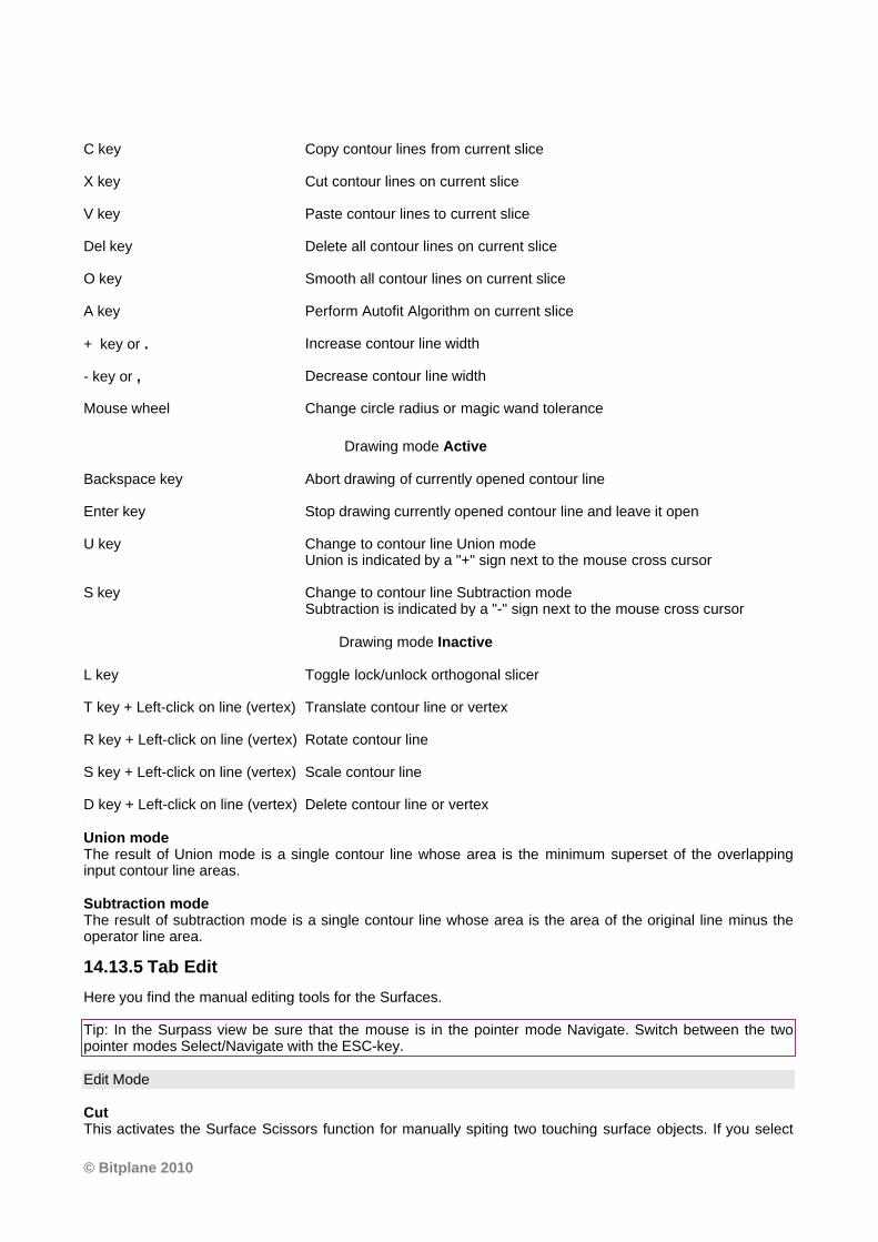
© Bitplane 2010
C key Copy contour lines from current slice
X key Cut contour lines on current slice
V key Paste contour lines to current slice
Del key Delete all contour lines on current slice
O key Smooth all contour lines on current slice
A key Perform Autofit Algorithm on current slice
+ key or . Increase contour line width
- key or , Decrease contour line width
Mouse wheel Change circle radius or magic wand tolerance
Drawing mode Active
Backspace key Abort drawing of currently opened contour line
Enter key Stop drawing currently opened contour line and leave it open
U key Change to contour line Union modeUnion is indicated by a "+" sign next to the mouse cross cursor
S key Change to contour line Subtraction modeSubtraction is indicated by a "-" sign next to the mouse cross cursor
Drawing mode Inactive
L key Toggle lock/unlock orthogonal slicer
T key + Left-click on line (vertex) Translate contour line or vertex
R key + Left-click on line (vertex) Rotate contour line
S key + Left-click on line (vertex) Scale contour line
D key + Left-click on line (vertex) Delete contour line or vertex
Union modeThe result of Union mode is a single contour line whose area is the minimum superset of the overlappinginput contour line areas.
Subtraction modeThe result of subtraction mode is a single contour line whose area is the area of the original line minus theoperator line area.
14.13.5 Tab Edit
Here you find the manual editing tools for the Surfaces.
Tip: In the Surpass view be sure that the mouse is in the pointer mode Navigate. Switch between the twopointer modes Select/Navigate with the ESC-key.
Edit Mode
Cut This activates the Surface Scissors function for manually spiting two touching surface objects. If you select
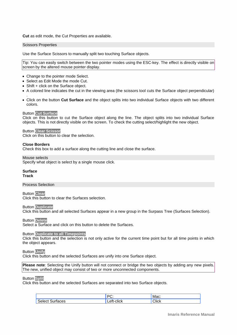
Imaris Reference Manual
Cut as edit mode, the Cut Properties are available.
Scissors Properties
Use the Surface Scissors to manually split two touching Surface objects.
Tip: You can easily switch between the two pointer modes using the ESC-key. The effect is directly visible onscreen by the altered mouse pointer display.
· Change to the pointer mode Select.· Select as Edit Mode the mode Cut. · Shift + click on the Surface object.· A colored line indicates the cut in the viewing area (the scissors tool cuts the Surface object perpendicular)
.· Click on the button Cut Surface and the object splits into two individual Surface objects with two different
colors.
Button Cut SurfaceClick on this button to cut the Surface object along the line. The object splits into two individual Surfaceobjects. This is not directly visible on the screen. To check the cutting select/highlight the new object.
Button Clear ScissorClick on this button to clear the selection.
Close BordersCheck this box to add a surface along the cutting line and close the surface.
Mouse selectsSpecify what object is select by a single mouse click.
SurfaceTrack
Process Selection
Button ClearClick this button to clear the Surfaces selection.
Button DuplicateClick this button and all selected Surfaces appear in a new group in the Surpass Tree (Surfaces Selection).
Button DeleteSelect a Surface and click on this button to delete the Surfaces.
Button Duplicate to all TimepointsClick this button and the selection is not only active for the current time point but for all time points in whichthe object appears.
Button UnifyClick this button and the selected Surfaces are unify into one Surface object.
Please note: Selecting the Unify button will not connect or bridge the two objects by adding any new pixels.The new, unified object may consist of two or more unconnected components.
Button SplitClick this button and the selected Surfaces are separated into two Surface objects.
PC: Mac: Select Surfaces Left-click Click
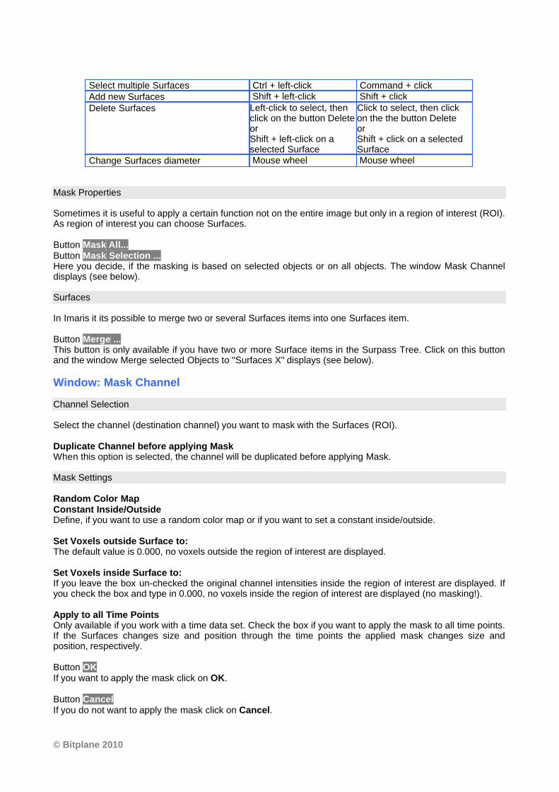
© Bitplane 2010
Select multiple Surfaces Ctrl + left-click Command + click Add new Surfaces Shift + left-click Shift + click
Delete Surfaces Left-click to select, thenclick on the button Deleteor Shift + left-click on aselected Surface
Click to select, then clickon the the button Deleteor Shift + click on a selectedSurface
Change Surfaces diameter Mouse wheel Mouse wheel
Mask Properties
Sometimes it is useful to apply a certain function not on the entire image but only in a region of interest (ROI).As region of interest you can choose Surfaces.
Button Mask All...Button Mask Selection ...Here you decide, if the masking is based on selected objects or on all objects. The window Mask Channeldisplays (see below).
Surfaces
In Imaris it its possible to merge two or several Surfaces items into one Surfaces item.
Button Merge ...This button is only available if you have two or more Surface items in the Surpass Tree. Click on this buttonand the window Merge selected Objects to "Surfaces X" displays (see below).
Window: Mask Channel
Channel Selection
Select the channel (destination channel) you want to mask with the Surfaces (ROI).
Duplicate Channel before applying MaskWhen this option is selected, the channel will be duplicated before applying Mask.
Mask Settings
Random Color MapConstant Inside/OutsideDefine, if you want to use a random color map or if you want to set a constant inside/outside.
Set Voxels outside Surface to:The default value is 0.000, no voxels outside the region of interest are displayed.
Set Voxels inside Surface to:If you leave the box un-checked the original channel intensities inside the region of interest are displayed. Ifyou check the box and type in 0.000, no voxels inside the region of interest are displayed (no masking!).
Apply to all Time PointsOnly available if you work with a time data set. Check the box if you want to apply the mask to all time points.If the Surfaces changes size and position through the time points the applied mask changes size andposition, respectively.
Button OKIf you want to apply the mask click on OK.
Button CancelIf you do not want to apply the mask click on Cancel.
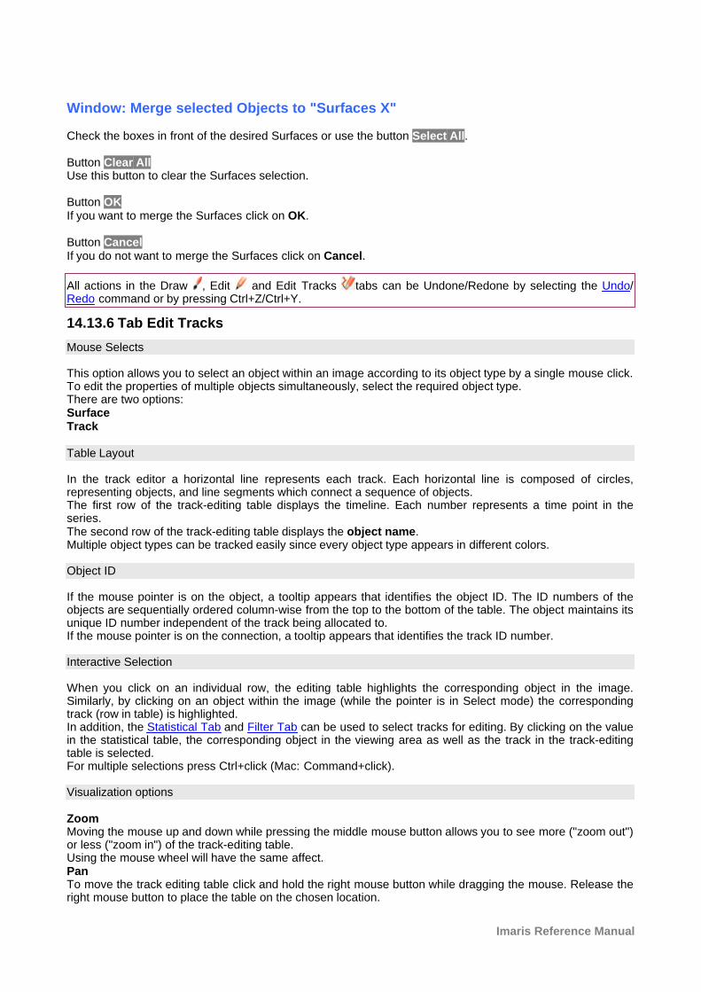
Imaris Reference Manual
Window: Merge selected Objects to "Surfaces X"
Check the boxes in front of the desired Surfaces or use the button Select All.
Button Clear AllUse this button to clear the Surfaces selection.
Button OKIf you want to merge the Surfaces click on OK.
Button CancelIf you do not want to merge the Surfaces click on Cancel.
All actions in the Draw , Edit and Edit Tracks tabs can be Undone/Redone by selecting the Undo/Redo command or by pressing Ctrl+Z/Ctrl+Y.
14.13.6 Tab Edit Tracks
Mouse Selects
This option allows you to select an object within an image according to its object type by a single mouse click.To edit the properties of multiple objects simultaneously, select the required object type. There are two options:SurfaceTrack
Table Layout
In the track editor a horizontal line represents each track. Each horizontal line is composed of circles,representing objects, and line segments which connect a sequence of objects.The first row of the track-editing table displays the timeline. Each number represents a time point in theseries.The second row of the track-editing table displays the object name. Multiple object types can be tracked easily since every object type appears in different colors.
Object ID
If the mouse pointer is on the object, a tooltip appears that identifies the object ID. The ID numbers of theobjects are sequentially ordered column-wise from the top to the bottom of the table. The object maintains itsunique ID number independent of the track being allocated to. If the mouse pointer is on the connection, a tooltip appears that identifies the track ID number.
Interactive Selection
When you click on an individual row, the editing table highlights the corresponding object in the image.Similarly, by clicking on an object within the image (while the pointer is in Select mode) the correspondingtrack (row in table) is highlighted. In addition, the Statistical Tab and Filter Tab can be used to select tracks for editing. By clicking on the valuein the statistical table, the corresponding object in the viewing area as well as the track in the track-editingtable is selected.For multiple selections press Ctrl+click (Mac: Command+click).
Visualization options
ZoomMoving the mouse up and down while pressing the middle mouse button allows you to see more ("zoom out")or less ("zoom in") of the track-editing table. Using the mouse wheel will have the same affect.PanTo move the track editing table click and hold the right mouse button while dragging the mouse. Release theright mouse button to place the table on the chosen location.
© Bitplane 2010
Time indicatorThe first row of the track-editing table displays the timeline. Each number represents a time point in theseries. The current time point is indicated by vertical line highlighted with in current selection color.
To modify the time point, do one of the following: 1. Moving the slider in the Time bar modifies its position in time and changes the time point in the trackeditor. 2. Clicking on the time point within the track-editing table automatically moves the time line indicator to thecorresponding point.Double clicking on the time indicator, fixes the position of the current time point at the center of thetrack-editing table, regardless of the selected zoom or pan options)
Editing
Track Editor has several features that help you modify your tracks
Add tracks
To set the starting point of a new connection first you have to select the object. Shift+left-click followed by a mouse movement on the object creates the new connection. To establish a connection, drag the edge to the target object. If valid, the target object is highlighted (red). Release the mouse button and the line segment clips automatically onto the new object, creating a newconnection between the two objects.
Please note: The new connection is only possible between the objects of the same type. If you release themouse button without being on a target object, the edge will disappear and a new connection will not beestablished.
A connection between objects of the same time point is also invalid.
Delete Tracks Edges
TracksSelect the track and press backspace to delete the whole track.
ConnectionsTo delete the connection, select the connection and press shift-click. The selected connection is deleted.
The process of deleting the connection splits the track. The first track part remains with the same ID numberand stops at the time point of the deletion. The second part consists of the remaining deleted objects and theconnections between them. It is automatically shifted to the bottom of the track-editing table and assigned anew track ID number.
Connect unconnected components
Manually added, or previously untracked objects are displayed as separated circles. The procedure ofcreating new connections and connecting the objects is unchanged.
Show selection (build working set)
This option allows you to work on subset of tracks.
Connect Track Button
Click this button to connect two existing tracks. Select two Spots in two different tracks at the subsequenttime points (just one Spot per time point) and click on the button Connect Track. The connection isautomatically created between all selected objects.
Disconnect Track Button
Select a object and click on the button Disconnect Track. The connection from the selected object to the next

Imaris Reference Manual
object in time sequence is deleted.
Correct Drift
If you have an object drift (e.g. a cell drift) during the image acquisition you can use the Correct Drift button tocorrect the drift for the whole data set.
The ImarisTrack tracks all objects in an image, even the objects that should be stationary.The Correct Drift function gives the user the opportunity:
1) to specify the tracks related to the stationary objects 2) to assign these objects as stationary objects and 3) to adjust the position of the rest of the image objects based on this selection.
As a result of drift correction, the entire image is transformed in such a way that the selected objects remainstationary and within the new image each objects’ position (changes) based on the correct draft algorithm.Within the new image, the true movement of the objects can be then detected relative to the stationaryobjects.
In the accordance with the selected for Result DataSets options. the new image coordinates are calculatedand displayed.
To make the Drift Correction on the data set the following steps are completed:· Select the tracks associated with the stationary objects· Select the algorithm for drift correction · Select the option for the Result data sets · Verify the selection and click on the OK button.
Please note: The drift correction changes the data set.
Based on the provided the track sub-selection the algorithm determines the new objects position for all timepoints.If the tracks are selected, the algorithm will be performed on the sub selection. Otherwise, every track of theimage is considered for calculations.
AlgorithmsThe Drift Correction is calculated based on the two algorithms, Translation and translation and rotation.
Translation
Upon translation, the object position is transformed to a straight line of identical orientation. Within the sametime point the relative distance of the objects is preserved.
Translation and rotation
Upon translation and rotation, the object position is transformed based on the image polar coordinates.Within the same time point the relative distance of the objects is preserved.
Please note: The number of the selected tracks affects the algorithm calculation.
Selection of a single track gives a complete description of a translation.Selection of a two tracks gives a minimum description of a translation and rotation algorithm (planar rotation). A better fit between the time points is achieved when three or more tracks are selected.
Result DataSet size
After completion of the drift correction, the algorithm uses the final position of the initial and resulting imageto create a final image. The new image coordinates are calculated in accordance with the size of the originaland new image.Select the Result data set option to determine which new image part will be displayed.
Crop largest common region
© Bitplane 2010
The final image will be the size of the common overlap between the original and the drift corrected image.Areas of the image that have been shifted outside these boundaries (to allow alignment) will be cropped fromthe final result.
New size equal to current size
The final image will be the same size as the original image. Areas of the image that have been shiftedoutside these boundaries (to allow alignment) will be cropped from the final result.
Include entire result
The final image will be the size of the combined area of the original and corrected image.Selecting the appropriate Result dataset size may speed up the data visualization. This is especiallyimportant with (with large data sets.)
Correct spots positions
Activate this parameter and the spots are automatically re-positioned after the drift correction. If this option isnot activated only the image volume is aligned.
All actions in the Draw , Edit and Edit Tracks tabs can be Undone/Redone by selecting the Undo/Redo command or by pressing Ctrl+Z/Ctrl+Y.
14.13.7 Tab Filter
Please note: Before using you have to add a filter to the list (see below: button Add)!
The Filter Type and its values define the section of interest, from this selection, which includes or excludesobjects based on a range of criteria. Select the filter type by selecting a variable from the drop-down list, andthen define the filter values, which will then limit the selection just to those objects that meet the set upcriteria. In Imaris you can choose two filter values, a Lower and a Higher filter value. The two filter values separate the data into three regions: above the higher value, below the lower value, andthe region in between. Objects with the relevant properties below the Lower filter value and objects with theproperties exceeding the Higher filter value will be excluded, and only those objects with qualities inside thedefined interval will be considered.
Please note if the value of the Lower filter value is set to be higher than that of the Higher filter value, theselected objects will be outside the defined interval. Only those objects meeting all the filter criteria areinteractively shown and instantly highlighted in the viewing area.
By using multiple filter types, more than one criterion can be specified for the data analyses.
Filters
Add ButtonTo add a new filter, click on the button Add and choose one of the Filter Types from the drop-down menu.Select the filtering type to be used in order to classify objects and specify the measurement of the criteria tobe used. The new filter appears in the list.
Delete ButtonSelect a filter in the list with a left mouse click and click on this button to delete the filter.
Filter Type
Select in the drop down list the filter you want to apply.
Filter category
A Category identifies, gathers and summaries a set of statistical values calculations of a particular Object
Imaris Reference Manual
Type. Statistical values associated with one object type are grouped in one category. Each category has anassociated button with graphical indications of Category type.In Imaris there are following Filter Categories: Surface , Surface Tracks , Spots , Spots Tracks ,
Dendrites , Dendrites Tracks , Filament , Filament Tracks , Spines , Spine Tracks , Point ,
Point Tracks , Cell , Cell Tracks , Nucleus , Nucleus Tracks , Vesicle and Vesicles Tracks
. These buttons allow you to choose the Category and determines the list of displayed statistical values.Clicking the button selects the corresponding category (the category button turns black) and the list ofstatistical values is displayed according to the selection.To remove the category from the list, re-click on the Category button. Re-clicking on the category buttondeselects Category and removes the selected statistical values from the list (turns the category button into alight gray color).
The exclamation mark sign indicates that the listed statistical parameter does not contain any value.
Lower and Upper Threshold
Activating/deactivating the Lower or Upper threshold option is done by clicking on the or button. The
Red button indicates that the threshold option is currently inactive, while the green button indicates anactive threshold.In order to activate the threshold option, click on the red button. To deactivate the threshold, click on thegreen circle again.
Automatic/Manual A/M buttonThe Automatic/Manual A/M button provides a single interaction point for the direct choice of the thresholdvalue adjustment.
When the lower/upper threshold values are not activated (the red button ) the corresponding A/M button islight gray indicating that threshold adjustment is unavailable. When the lower/upper threshold option is
activated (the green button ), the corresponding A/M button turns black.
After the first threshold activation, as a default, an Automatic threshold value is activated . Clicking onthe Automatic/Manual button allows you to switch between an Automatic and a Manual threshold adjustmentmode. The A/M button provides a visual feedback as an indication of the selected threshold adjustment
mode. Clicking on the A/M button changes the appearance of the A/M button form indicating an
activated Automatic threshold to indicating a Manual threshold. Clicking on the histogram automatically activates a Manual threshold adjustment.
Lower Threshold
AutomaticThe initial threshold value is automatically computed.ManualDefine the threshold by clicking into the histogram or by entering the value directly in the data field. Eithertype in the value or click into the histogram to move the colored line and then a reduced/enlarged set ofobjects are visualized.
Higher Threshold
AutomaticThe initial threshold value is automatically computed.ManualDefine the threshold by clicking into the histogram or by entering the value directly in the data field. Eithertype in the value or click into the histogram to move the colored line and then a reduced/enlarged set ofobjects are visualized.
Histogram
In the histogram the regions above and below the threshold values are displayed in white, while the regionwithin the threshold is displayed in yellow. To change the automatically set threshold values, select the optionManual. By clicking into the histogram you move the colored line and the reduced/enlarged set of objects. To
© Bitplane 2010
change the Lower threshold value left click on the histogram and drag the yellow line. To change the Higher threshold value right click on the histogram and move the line. Move the line to theright to increase the threshold and to decrease the threshold move the line to the left. These changes areinstantly visible in the viewing area.The numerical range of the statistics value (e.g. Quality)and the number and percentage of objects that fallinto the particular filtering class are displayed at the bottom of the threshold histogram.
Duplicate Selection to New Surfaces ButtonClick on this button and all selected objects are copied to a new group. The new group displays in theSurpass Tree.
See also:Surpass View - Overview - Surpass Tree
14.13.8 Tab Statistics
Surfaces statistics are automatically computed. For the statistical values please refer to the chapter MenuEdit - Preferences... - Statistics - Surfaces. The Statistics tab collects and displays the image's statisticalvalues in Imaris. The Statistics tab enables us to understand and compare different datasets throughsummarized statistical values and graphical data presentations. Several types of statistical tools enable convenient organization and analysis of heterogeneous statisticaldata. The Statistics View is configured as follows: a) Overall b) Detailedc) SelectionIn the statistical dataset the first column contains the name of the variable, followed by columns withcalculated statistical data. Corresponding statistical variable values are presented in rows. To sort the columns click on the arrow in column heading. Click again to reverse the sort.
Overall Tab
Output of the Overall statistics provides an overview of the image's single determining variables. Onlystatistics that are not measured on a per-object basis are displayed here.
Category
A Category identifies, gathers and summaries a set of statistical values calculations of a particular ObjectType. Statistical values associated with one object type are grouped in one category. Each category has anassociated button with graphical indications of Category type.In Imaris there are following Filter Categories: Surface , Surface Tracks , Spots , Spots Tracks ,
Dendrites , Dendrites Tracks , Filament , Filament Tracks , Spines , Spine Tracks , Point ,
Point Tracks , Cell , Cell Tracks , Nucleus , Nucleus Tracks , Vesicle and Vesicles Tracks
. These buttons allow you to choose the Category and determines the list of displayed statistical values.Clicking the button selects the corresponding category (the category button turns black) and the list ofstatistical values is displayed according to the selection.To remove the category from the list, re-click on the Category button. Re-clicking on the category buttondeselects Category and removes the selected statistical values from the list (turns the category button into alight gray color).
The exclamation mark sign indicates that the listed statistical parameter does not contain any value.
Detailed Tab
A pull down list offers three types of Detailed statistical calculations: Specific ValuesAverage ValuesAll Values
Imaris Reference Manual
Time Plots The values displayed are always for the current time point. Selecting a variable that changes over timecreates a plot of selected values as a time function. The statistical variable value is plotted on the verticalaxis and the time is plotted on the horizontal axis. The current time point is indicated with a black vertical line.Each time value is displayed as a point. Click inside the plot and move the time line. Moving the line changesthe time point. Altering the time point changes the variable value and the image.Multiple value selection, available by Ctrl+ click, will plot a superimposed second selected value over the firstone.
Interactive two-way SelectionA click on an individual row of the table highlights the corresponding object in the image. Similarly, by clickingon an element in the image (while the pointer is in Select mode) the corresponding row in table will behighlighted. A possibility of multiple selections is available by pressing Ctrl+click (Mac: Command+click).
Specific Values In the Specific Values, a second pull down list at the top of the window displays available specific statisticalvalues. Select the variable and a list of values will be displayed.Object Statistical Annotation option is available for Specific values parameters.
Average valuesThe Average table contains values determined on the basis of all values within a set of the selected variable.Columns are labeled as follows:Min (Minimum)- the smallest value within a set of values of the selected variable Max (Maximum)- the largest value within a set of values of the selected variable Mean – value of the sum of all values divided by number of values within a set Std Dev (Standard deviation)- a measure of the values distribution around the mean values Median- the middle value of the sorted set of variablesSum- the sum of all values within a variable setCount- number of values within a setUnit- variable unit Level/Distance
The black line on the time plot indicates where the mean value lies, the red indicates the median, the lightgray area shows the range between the min and max values and dark gray region labels the standarddeviation range with error bars.
Statistical variable classification: 1. Statistical variables associated with objects (Cells, Nucleus, Vesicles -volume, area, intensity values,position, speed, displacement) have values at every time point. Therefore for these variables the Averagevalues are displayed per time point. The changing the time points, statistical variable values and images areconsequently changed.2. Statistical values with data associated with Tracks (track duration, track volume mean, track displacementlength, track intensity) are not time dependent.
All valuesIf the option All values is selected for the detailed tab, all values will be displayed. Even though this option isalways readily available, it is discouraged to use it in order to avoid data clutter.Object Statistical Annotation option is available for Specific values parameters.
Selection Tab
Statistical tables for a selected object will be displayed. Change to the pointer mode Select and click on animage element that has been detected/segmented. A possibility of multiple selections is available byCtrl+click (Mac: Command-click).A pull down list offers three types of statistical calculations from a Selection:Specific ValuesAverage ValuesAll Values
Time Plots
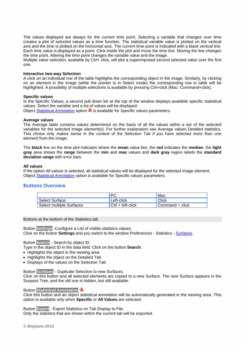
© Bitplane 2010
The values displayed are always for the current time point. Selecting a variable that changes over timecreates a plot of selected values as a time function. The statistical variable value is plotted on the verticalaxis and the time is plotted on the horizontal axis. The current time point is indicated with a black vertical line.Each time value is displayed as a point. Click inside the plot and move the time line. Moving the line changesthe time point. Altering the time point changes the variable value and the image.Multiple value selection, available by Ctrl+ click, will plot a superimposed second selected value over the firstone.
Interactive two-way SelectionA click on an individual row of the table highlights the corresponding object in the image. Similarly, by clickingon an element in the image (while the pointer is in Select mode) the corresponding row in table will behighlighted. A possibility of multiple selections is available by pressing Ctrl+click (Mac: Command+click).
Specific valuesIn the Specific Values, a second pull down list at the top of the window displays available specific statisticalvalues. Select the variable and a list of values will be displayed.Object Statistical Annotation option is available for Specific values parameters.
Average valuesThe Average table contains values determined on the basis of all the values within a set of the selectedvariables for the selected image element(s). For further explanation see Average values Detailed statistics.This choice only makes sense in the context of the Selection Tab if you have selected more than oneelement from the image.
The black line on the time plot indicates where the mean value lies, the red indicates the median, the lightgray area shows the range between the min and max values and dark gray region labels the standarddeviation range with error bars.
All valuesIf the option All values is selected, all statistical values will be displayed for the selected image element. Object Statistical Annotation option is available for Specific values parameters.
Buttons Overview
PC: Mac: Select Surface Left-click Click Select multiple Surfaces Ctrl + left-click Command + click
Buttons at the bottom of the Statistics tab
Button Settings -Configure a List of visible statistics values. Click on the button Settings and you switch to the window Preferences - Statistics - Surfaces.
Button Search - Search by object ID.Type in the object ID in the data field. Click on the button Search. · Highlights the object in the viewing area· Highlights the object on the Detailed Tab· Displays of the values on the Selection Tab
Button Surfaces - Duplicate Selection to new Surfaces.Click on this button and all selected elements are copied to a new Surface. The new Surface appears in theSurpass Tree, and the old one is hidden, but still available.
Button Statistical Annotation Click this button and an object statistical annotation will be automatically generated in the viewing area. Thisoption is available only when Specific or All Values are selected.
Button Export - Export Statistics on Tab Display to File. Only the statistics that are shown within the current tab will be exported.
Imaris Reference Manual
Button Export - Export selected Data for plottingExports the selected statistical value for plotting. The selected value has to be time dependent.With a click on the button Export the Export Statistics window opens. Select the file type (CommaSeparated Values *.csv, Excel file *.xls, or Excel XML *.xlm). If you select MS Excel as file type, the programstarts automatically.
Button Export - Export All Statistics to File. All of the statistics (that are enabled in the statistics settings) will be exported.With a click on the button Export the Export Statistics window opens. Select the file type (CommaSeparated Values *.csv, Excel file *.xls, or Excel XML *.xlm). If you select MS Excel as file type, the programstarts automatically and the sheets show up one after another (this will take several seconds).
See also:Menu Edit - Preferences... - Statistics - Surfaces
14.13.8.1 Statistical Annotations
Statistical annotations provides the opportunity to view and annotate image objects with the statistical datavalues. Using this function, the individual objects in an image are labeled with the specified statistical valuesand the statistical data is displayed directly in the viewing area Imaris objects can be labeled with a set of any number of the user-defined statistical values.The Statistical Annotation button provides a convenient interface in order to label the object with thestatistical data. Click this button and an object statistical annotation will be automatically generated in theviewing area. The selected object is annotated for all time points with the specified statistical values.
How to add Statistical Annotation
In the Statistical tab choose the Detailed or Selection Tab. In the viewing area select the object or group of objects. Change to the pointer mode Select and click on animage object that has been detected/segmented. For multiple selections press Ctrl+click (Mac:Command-click)In the Detailed or Selection Tab a pull down list offers Specific Values or All values as types of statisticalparameters. Select the statistical value associated with the particular object type you are working with.Press the Statistical Annotation button .
In the viewing area the object label appears showing selected statistical values as a statistical annotation.
The statistical annotation shows by default the name of the selected statistical parameter and its value.The color white displays the text of annotations associated with statistical values.
For a single object, all selected statistical parameters are placed in the same annotation box. Once the objectis labeled, selecting the additional statistical parameter updates the object statistical annotation; the newparameter and its value is added in the viewing area.If the image is a time series, the statistical annotation will be visible in the viewing area for all time points.Selecting a statistical variable that changes over time creates an statistical annotation that consequentlychanges with every time point.The statistical annotation displays values always for the current time point.
The InPress options will allow you to modify and specify the contents and format of the object labels.
To modify and adjust the statistical label click on the Icon InPress , press Ctrl + Shift + P, or in the menubar select File – InPress.
14.13.9 Tab Color
Tab Color edit, manage and assign colors material to the Surfaces or Tracks.
Object Type
Choice of Object type is presented in drop down window. Select either Surfaces or Tracks and depending onthe chosen object type selection of the variables is listed.
© Bitplane 2010
For Object Type Surfaces two color types are available:BaseStatistics Coded
For Object Type Tracks three color types are available:BaseStatistics CodedTime Mapped
14.13.9.1 Color Type-Base
Tab Color edit, manage and assign material colors of a Surfaces/Track.
RGB
The RGB color model is an additive color model in which Red, Green and Blue are combined together toreproduce an array of colors. The color values may be changed either by clicking on the color wheel to selecta color or by direct numeric entry for the Red, Blue or Green component (values range from 0 to 1).
Light reflection
Quality of the object material is further characterized by reflection properties. Diffusion- diffuses reflection of a matte, uneven material.Specular- defines reflection of highly reflective materials. The brighter a specular map is, the more shine isapplied to the object. Default setting has no specular intensity.Emission- light emitted from the material defines the self-illumination. Default setting emits no light.
Transparency
Transparency- defines the amount of light allowed to pass through an object. Click this tool to change thepercentage from 0% (complete opacity) to 100% (complete image transparency).
Palette
Palette- this option provides a system of preset colors organized into color schemes. In the Palette, colors are labeled and grouped together. The scrolling window contains the 14 colorcombination groups (Custom, artdeco, autumn, glass, metal, neon, rococo, santafe, sheen, silky, spring,summer, tropical, winter). Examples of colors in a selected group are displayed in the attached rectangulararea. If a custom color has been defined on the RGB tab, it can be added to the Custom palette with the Addto Palette button. After being added, these color choices are stored and can be used with other Imarisobjects.
14.13.9.2 Color Type-Statistics Coded
Statistics Coded
Depending on the object type selection (either Surfaces or Tracks) the Statistical variable selection is listed inthe drop down window. For example, if Surfaces is chosen as the Object type, available Statistical type willbe the Surface linked variable. Similarly, Statistical variables for Tracks will be listed, if Object type isselected to be Tracks.
Statistics Colorbar Properties
Statistics colorbar are displayed in the viewing area. The upper one is the colorbar range for Surfaces andlower one is the colorbar for the Tracks.
Show ColorbarCheck the box to see the statistics colorbar in the viewing area.
Show Title
Imaris Reference Manual
Check this box to see the title in the statistics colorbar.
Show RangeCheck this box to see the range in the statistics colorbar.
Font color in colorbar is adjustable by selecting a color within the color map.
Colormap
Button ResetClick the Reset button to set the image back to the original values.
Button Load …Click on the button Load to display the Import Color Table File color window. Enter the path and therequested File name and/or File type and click Open. The selected file is loaded and displayed.
Colormap range
Colormap range-specify the limits for colorbar. Min - lower color limitMax - upper color limitButton AutoClick the button Auto to detect the system the real min and max values and sets the Max. and Min. limitsautomatically to these values.
Transparency
Transparency defining amount of light allowed to pass through. Click this tool to change the percentagefrom 0% (complete opacity) to 100% (complete image transparency).
14.13.9.3 Color Type-Time Mapped
Time MappedThis option is only available when Tracks (see above) is selected as Object Type. The color range for theTracks goes from blue to white to the range of time points.
Transparency
Transparency defining amount of light allowed to pass through. Click this tool to change the percentagefrom 0% (complete opacity) to 100% (complete image transparency).
14.14 Volume
How to Add a new Volume?
· Select menu Surpass - Volume.
The Surpass Tree list is automatically updated and in the Volume - Properties the Settings parameter aredisplayed. A data set can have only one volume.
14.14.1 Display Adjustments
To set the correct Display Adjustments for the Volume rendering of your data set please refer to chapterMenu Eidit - Show Display Adjustment.
© Bitplane 2010
14.14.2 Tab Settings
Mode
MIP (max) In the Maximum Intensity Projection mode only the brightest point (the point with maximum intensity) of alllayers along the viewing direction displays. If your data set has more then one channel the combination colordisplays. A layer in the data set with high red and high green intensity displays yellow.
Normal ShadingThe result of the normal shading is a depth effect on the screen. The surfaces turned away from the lightsource appear darker.
MIP (min) A Maximum Intensity Projection with minimum intensity of all layers along the viewing direction.
Blend The result of the bland mode is a depth effect on the screen. One effect of the blend mode is, that theborders appear darker. In the blend mode all values along the viewing direction including their transparencyare used for the calculation.
Shadow ProjectionThe result of the shadow projection is a depth effect on the screen. An object between light source and thesurface you look at projects a shadow.
If Shadow Projection is selected, the parameter Fix Light(s) to Data Set is available.
Fix Light(s) to Data SetCheck the box to fix the x-, y-, and z-axes to the same side when navigating the object. When the box isun-checked, the light source is fixed to a particular position in space and remains in place when the objectmoves or rotates.
This check-box is only available, if Shadow Projection is selected.
Rendering Quality
If the rendering quality is set to 1.000, then 1pixel represents 1 voxel. If you decrease the rendering qualitythe image becomes coarse-grained.
View Aligned PlanesCheck this box to see the display planes. Examine the planes while rotating the data set in the viewing area.
See also:Preface - Terminology
14.14.3 Tab Draw
Volume Painter
On the tab Draw you can find the settings for the Volume Painter. Use this Volume Painter to adjust the voxelintensities before you do a segmentation based on Surfaces, Spots, or Filament. (If an automatic algorithm isnot able to separate two objects, the intensity between these two objects can be "erased" in advance.) Youcan draw disks, spheres, or hallow spheres into the selected image channel.
· First select the desired channel and painter shape.· Rotate the view to execute a vertical cut. · Then customize the painter settings. · Change to the pointer mode Select. · Move the cursor to the desired position. · Hold down the Shift-key and click to add the shape.
Imaris Reference Manual
· In the viewing area you see a preview of the painter tool. · To re-edit a shape use the point selection. · Set intensity to 0 to erase a region, or set the intensity to 255 to fill a region.· To fix the shape click on the button Set Intensity.
Please note: The button Set Intensity changes the data set.
Selected Channel
Select the respective source channel.
Painter Shape
Here you select the painter shape.
DiskThe painter is disk shaped. In the settings selection adjust the diameter, width and intensity of the disk (seebelow).
SphereThe painter is a sphere. In the settings selection adjust the diameter and intensity of the sphere (see below).
Hollow SphereThe painter is a hollow sphere. In the settings selection adjust the diameter and intensity of the hollow sphere(see below).
Selection
DiameterHere you select the diameter of a disk, sphere, and hollow sphere. If your mouse has a wheel, you can usethe wheel to adjust the diameter.
WidthHere you select the width of a disk.
IntensityHere you select the painter shape intensity. The shape preview in the viewing area changes accordingly. Ifyou want to cut parts out of the channel select 0 as intensity value.
Button Set IntensityIn the last step you click on this button to fix the shapes. The button Set Intensity changes the data set and itis not possible to re-edit the shapes again.
Button Delete AllClick on this button to delete all inserted shapes in the preview.
Selected Point
You can use the following data fields and the button Delete to re-edit or delete a selected point.
Position [um] X, Y, ZTo select a point change to the pointer mode Select and click on a point. The color of the selected pointchanges. The point position displays in the x, y, and z data field. To move the point click on the new positionin the viewing area or edit the x, y, or z data field.
Button DeleteClick on this button to delete the selected point.
© Bitplane 2010
14.14.4 Tab Statistics
Volume statistics are automatically computed. For the statistical variable values please refer to the chapterMenu Edit - Preferences... - Statistics - Volume.Statistic tab collects and displays image statistical values inImaris. Statistic tab enable us to understand and compare different datasets through summarized statisticalvalues and graphical data presentations. Several types of statistical tools enabling convenient organization and analysis of heterogeneous statisticaldata. Statistical View is configured as follows: a) Overall b) Detailedc) SelectionIn statistical dataset the first column contains the name of the variable, followed by columns with calculatedstatistical data. Corresponding statistical variable values are presented in rows. To sort columns click on the arrow in column heading. Click again to reverse the sort.
Overall Tab
Output of the Overall statistics provides an overview of the image single determining variables.
Buttons at the bottom of the Statistics tab
Button Settings - Configure List of visible statistics values. Click on the button Settings and you switch to the window Preferences - Statistics - Volume.
Button Search - Search by object ID.Type in the object ID in the data field. Click on the button Search. · Highlight the object in viewing area· Highlight the object on the Detailed Tab· Display of the values on the Selection Tab
Button Surfaces - Duplicate Selection to new Surfaces.Click on this button and all selected objects are copied to a new group. The new group displays in theSurpass Tree.
Button Export - Export Statistics on Tab Display to File.
Button Export - Export selected Data for plottingExports the selected statistical value for plotting. The selected value has to be time dependent.With a click on the button Export the Export Statistics window opens. Select the file type (CommaSeparated Values *.csv, Excel file *.xls, or Excel XML *.xlm). If you select MS Excel as file type, the programstarts automatically.
Button Export - Export All Statistics to File. With a click on the button Export you open the Window Export Statistics. Select the file type (CommaSeparated Values *.csv, Excel file *.xls, or Excel XML *.xlm). If you select MS Excel, the program startsautomatically and the sheets show up one after another (this will take several seconds).
See also:Menu Edit - Preferences... - Statistics - Volume
15 Animation
The Key Frame Animation function defines several subsequent views (key frames) of your image, which willbe used to create an animation. Imaris generates smooth transitions between the selected views byinterpolation.
How to Open the Key Frame Animation Window?
· Click on the icon in the Main toolbar.
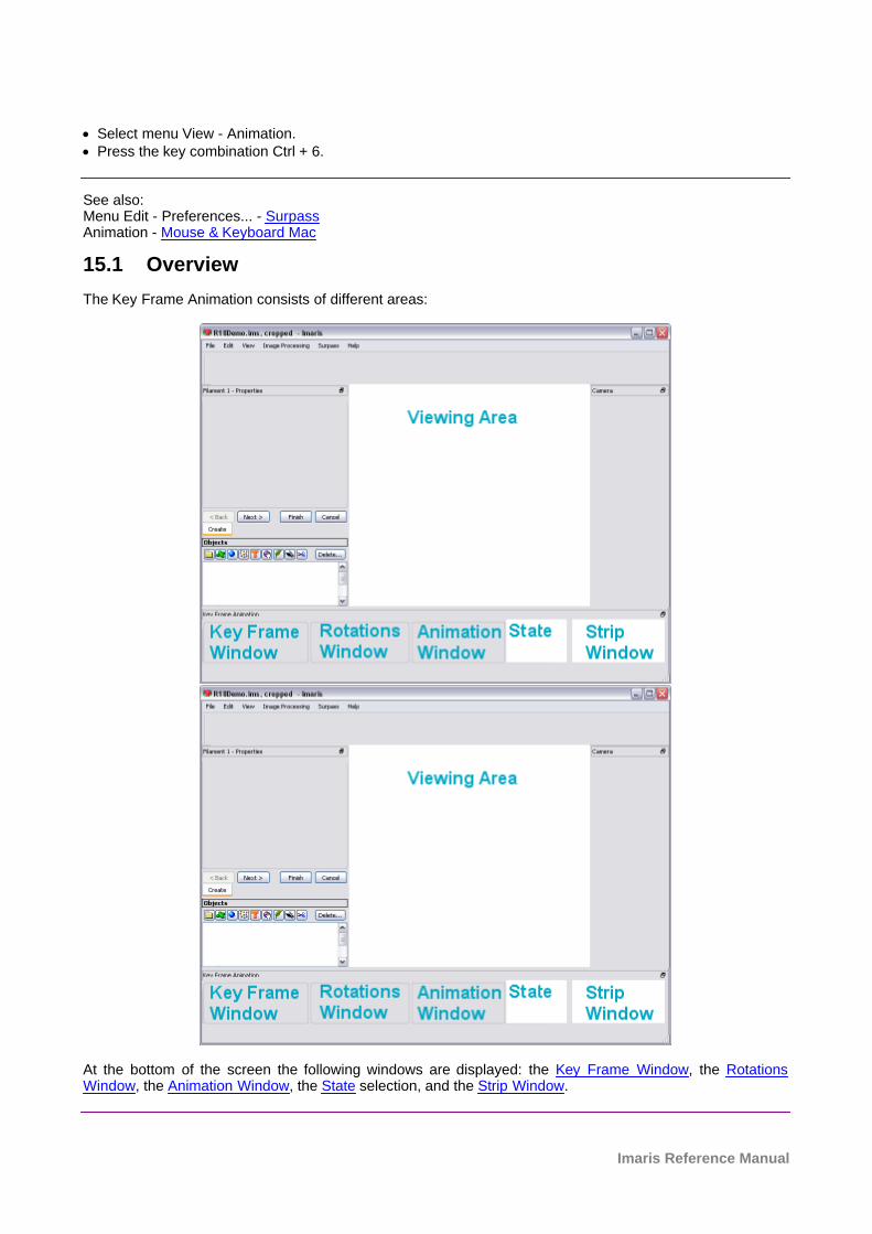
Imaris Reference Manual
· Select menu View - Animation.· Press the key combination Ctrl + 6.
See also:Menu Edit - Preferences... - SurpassAnimation - Mouse & Keyboard Mac
15.1 Overview
The Key Frame Animation consists of different areas:
At the bottom of the screen the following windows are displayed: the Key Frame Window, the RotationsWindow, the Animation Window, the State selection, and the Strip Window.
© Bitplane 2010
15.2 Key Frame Window
In the Key Frame window you define and manage the key frames of your movie.
Button AddUse this button to insert user-defined key frames in the strip sequence.
Button Modify Use this button to modify user-defined key frames in the strip sequence.
Button DeleteUse this button to delete user-defined key frames in the strip sequence.
Button Delete AllClick on this button to delete all user-defined key frames in the Strip window.
Large spaces between the user-defined key frames (thick blue lines) will cause that section of the movie toplay more slowly. Placing the lines close together will cause that section of the movie to play more quickly.Use this button to set a constant speed throughout the entire movie.
Button II<Button II>With the arrow buttons you step to the previous (arrow to the left) or next (arrow to the right) user-defined keyframe.
Buttons Overview
Add Add new user-defined key frame Mod. Modify active, user-defined key frame Del Delete active, user-defined key frame Del. All Delete all key frames II< Go to Previous user-defined key frame II> Go to Next user-defined key frame
For the complex use of these buttons please refer to chapter Animation - Strip Window.
See also:Animation - Create Animation
15.3 Rotations Window
Use the templates to quickly define standard camera motions for the key frame animation system.
TemplatesSelect one of the predefined templates. The key frames are inserted automatically. Click on the button Playto see the animation.
Button CustomClick on this button to display the Custom Rotation window to freely define the rotation (see below).
Space
ScreenThe rotation axis is associated to the x-, y-, and z-axis of the screen.
WorldThe rotation axis is associated to the x-, y-, and z-axis of the data set.
Imaris Reference Manual
Axis
XYZTurn along the x-, y-, or z-axis.
Direction
+Turn to the left.
-Turn to the right.
Angle
Select or type in the desired angle.
Button OK Click on this button to accept the changes.
Button CancelClick on this button to cancel the changes.
15.4 Animation Window
FramesThe number in the filed Frames indicates the number of thin blue lines within the Strip Panel. This numberdefines the duration of animations.
Button Settings ...To open and adjust the Key Frame settings click on this button. For details please refer to chapter Menu Edit- Preferences... - Surpass.
Button >Click on this button (arrow to the right - Play/Pause) to start the movie preview. To pause the movie previewre-click on this button.
Button OTo record the movie click on this button (red dot - Record). Selecting this button the Save As Movie windowis displayed (see below).
Window: Save as Movie Window
File nameEnter a file name.
Save as typeSelect the desired file type (QuickTimeMovie, TIFF series, or AVI).
Movie Settings
Compression FactorSelect a compression factor between 0 (high quality) and 100 (low quality), the default setting is 5. Use theslider to set the compression factor between 0 and 100. A lower factor results in a lower compression andtherefore a better quality, but also in a larger movie file.
Frame Rate
© Bitplane 2010
Define how many frames are displayed per second.
QTVR Settings
The QuickTimeVR Settings are not available.
Add to ImageAccess databaseCheck the box to add the file to the ImageAccess database.
Play Movie with default Media Player when finishedCheck the box to play the movie with the default media player when finished.
Menu Edit - Preferences... - Surpass (default Key Frame settings)Surpass View - Overview - QuickTimeVR
15.5 Play Back State
In the State selection you can adjust the play back settings.
Camera· Check: Play back the previously recorded Camera positions for each key frame.· Un-check: Do not play back the recorded Camera positions. The Camera stays in the same position. You
can change the Camera position manually while playing the animation.
Time Points· Check: Play back the previously recorded Time Points for each key frame.· Un-check: Do not play back the recorded Time Points. The Time Points do not automatically change
during the animation. You can change the Time Points manually while playing the animation.
Colors· Check: Play back the previously recorded Colors for each key frame.· Un-check: Do not play back the recorded Colors. The Colors do not automatically change during the
animation. You can change the Colors manually while playing the animation.
Display Adjustments· Check: Play back the previously recorded Display Adjustments for each key frame.· Un-check: Do not play back the recorded Display Adjustments. The Display Adjustments do not
automatically change during the animation. You can change the Display Adjustments manually whileplaying the animation.
Clipping Plane (Position)· Check: Play back the previously recorded Clipping Plane positions for each key frame.· Un-check: Do not play back the recorded Clipping Plane positions. The Clipping Plane positions do not
automatically change during the animation. You can change the Clipping Plane positions manually whileplaying the animation.
Orthogonal Slicer (Position)· Check: Play back the previously recorded Orthogonal Slicer positions for each key frame.· Un-check: Do not play back the recorded Orthogonal Slicer positions. The Orthogonal Slicer positions do
not automatically change during the animation. You can change the Orthogonal Slicer positions manuallywhile playing the animation.
Oblique Slicer (Position)· Check: Play back the previously recorded Oblique Slicer positions for each key frame.· Un-check: Do not play back the recorded Oblique Slicer positions. The Oblique Slicer positions do not
automatically change during the animation. You can change the Oblique Slicer positions manually whileplaying the animation.
Objects Show/Hide (Object Visibility)
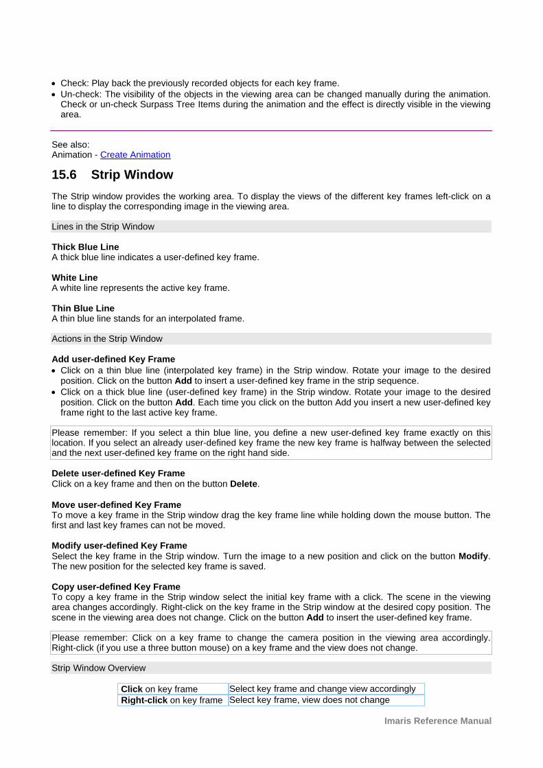
Imaris Reference Manual
· Check: Play back the previously recorded objects for each key frame.· Un-check: The visibility of the objects in the viewing area can be changed manually during the animation.
Check or un-check Surpass Tree Items during the animation and the effect is directly visible in the viewingarea.
See also:Animation - Create Animation
15.6 Strip Window
The Strip window provides the working area. To display the views of the different key frames left-click on aline to display the corresponding image in the viewing area.
Lines in the Strip Window
Thick Blue LineA thick blue line indicates a user-defined key frame.
White LineA white line represents the active key frame.
Thin Blue LineA thin blue line stands for an interpolated frame.
Actions in the Strip Window
Add user-defined Key Frame· Click on a thin blue line (interpolated key frame) in the Strip window. Rotate your image to the desired
position. Click on the button Add to insert a user-defined key frame in the strip sequence.· Click on a thick blue line (user-defined key frame) in the Strip window. Rotate your image to the desired
position. Click on the button Add. Each time you click on the button Add you insert a new user-defined keyframe right to the last active key frame.
Please remember: If you select a thin blue line, you define a new user-defined key frame exactly on thislocation. If you select an already user-defined key frame the new key frame is halfway between the selectedand the next user-defined key frame on the right hand side.
Delete user-defined Key FrameClick on a key frame and then on the button Delete.
Move user-defined Key FrameTo move a key frame in the Strip window drag the key frame line while holding down the mouse button. Thefirst and last key frames can not be moved.
Modify user-defined Key FrameSelect the key frame in the Strip window. Turn the image to a new position and click on the button Modify.The new position for the selected key frame is saved.
Copy user-defined Key FrameTo copy a key frame in the Strip window select the initial key frame with a click. The scene in the viewingarea changes accordingly. Right-click on the key frame in the Strip window at the desired copy position. Thescene in the viewing area does not change. Click on the button Add to insert the user-defined key frame.
Please remember: Click on a key frame to change the camera position in the viewing area accordingly.Right-click (if you use a three button mouse) on a key frame and the view does not change.
Strip Window Overview
Click on key frame Select key frame and change view accordingly
Right-click on key frame Select key frame, view does not change
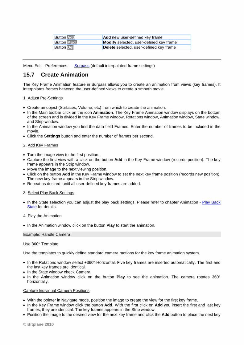
© Bitplane 2010
Button Add Add new user-defined key frame Button Mod. Modify selected, user-defined key frame Button Del Delete selected, user-defined key frame
Menu Edit - Preferences... - Surpass (default interpolated frame settings)
15.7 Create Animation
The Key Frame Animation feature in Surpass allows you to create an animation from views (key frames). Itinterpolates frames between the user-defined views to create a smooth movie.
1. Adjust Pre-Settings
· Create an object (Surfaces, Volume, etc) from which to create the animation.· In the Main toolbar click on the icon Animation. The Key Frame Animation window displays on the bottom
of the screen and is divided in the Key Frame window, Rotations window, Animation window, State window,and Strip window.
· In the Animation window you find the data field Frames. Enter the number of frames to be included in themovie.
· Click the Settings button and enter the number of frames per second.
2. Add Key Frames
· Turn the image view to the first position. · Capture the first view with a click on the button Add in the Key Frame window (records position). The key
frame appears in the Strip window. · Move the image to the next viewing position. · Click on the button Add in the Key Frame window to set the next key frame position (records new position).
The new key frame appears in the Strip window. · Repeat as desired, until all user-defined key frames are added.
3. Select Play Back Settings
· In the State selection you can adjust the play back settings. Please refer to chapter Animation - Play BackState for details.
4. Play the Animation
· In the Animation window click on the button Play to start the animation.
Example: Handle Camera
Use 360° Template
Use the templates to quickly define standard camera motions for the key frame animation system.
· In the Rotations window select +360° Horizontal. Five key frames are inserted automatically. The first andthe last key frames are identical.
· In the State window check Camera.· In the Animation window click on the button Play to see the animation. The camera rotates 360°
horizontally.
Capture Individual Camera Positions
· With the pointer in Navigate mode, position the image to create the view for the first key frame. · In the Key Frame window click the button Add. With the first click on Add you insert the first and last key
frames, they are identical. The key frames appears in the Strip window. · Position the image to the desired view for the next key frame and click the Add button to place the next key
Imaris Reference Manual
frame.· Repeat as desired, until all user-defined key frames are added. · In the State window check Camera.· To preview the movie, click in the Animation window on the button Play. The camera position changes
automatically.
Move the Camera Position Manually During the Play Back
· Create an animation.· In the State window un-check Camera.· Play the animation and change the Camera position during the play back manually.
Example: Handle the Orthogonal Slicer
Individual Orthogonal Slicer Positions
· Add the Surpass Tree Item Orthogonal Slicer and check the box in the Surpass Tree. · Adjust the Orthogonal Slicer for the first key frame and click on the button Add. · Move the Orthogonal Slicer before you add the next key frame and so on. · In the State window check Orthogonal Slicer.· Play the animation. The Orthogonal Slicer position changes automatically.
Change Orthogonal Slicer Position Manually During the Play Back
· Create an animation.· In the State window un-check Orthogonal Slicer.· Play the animation and change the Orthogonal Slicer position during the play back manually.
See also:Animation - OverviewAnimation - Key Frame WindowAnimation - Rotations WindowAnimation - Animation WindowAnimation - Play Back StateAnimation - Strip WindowAnimation - Save Animation
15.8 Save Animation
When you are satisfied with the movie, there are two possibilities to save the animation; either as an ImarisScene File or as a movie-file.In Imaris as Scene FileWhenever you save the Scene File in Imaris, the actual animation is saved automatically as part of theScene File. Open the menu File and select Export Scene and click on Save.
Save Different Animations in Different Scene FilesSaving different animations of the same data set requires saving of different Scene Files. After generating anew movie by the Key Frame Animation, rename each time the Scene File, e.g. add "Movie" at the end of theScene File name. Open the menu File and select Export Scene... . In the dialog window type in the newScene File name (e.g. PyramidalCellSceneAMovie.imx) and click on Save.
Record the Animation as Movie
To save the animation as movie click in the Animation window on the button Record (red dot). The Save AsMovie dialog window is displayed on screen. As File name type in the corresponding Scene File name, selectthe file type and choose the Movie Settings. Click on Save.
The Save as type option allows you to select the movie output file format and save the settings as a presetfor future use.
© Bitplane 2010
Imaris lets you save and create movie files on any platform. The movie file type specifies the video formatand predetermines the codes required to view saved animation. To playback the movie you must use the appropriate Media player for the selected movie file type.
Available Movie File Formats are:
MPEG-1 Movie (*.mpg)MPEG-4 Movie (*.mp4)AVI Movie (*.avi)WMV Movie (*.wmv)Quicktime Movie (*.mov)Flash Movie (*.flv)Raw Movie (*.avi)Tiff (series) (*.tif, *.tiff)Quicktime Virtual Reality Movie (*.mov)
Please note: The number and type of media player codes available depends on your operating systemversion, video card, and other software installed on your system.
If you have experienced problems with viewing the created animation files we recommend installing the freeand platform independent, VLC player.
See also:Menu File - Export Scene...Surpass View - Overview - Scene File Concept Surpass View - Overview - Quick TimeVRAnimation - Animation Window (Button Record)
15.9 Mouse & Keyboard PC
Animation Mouse & Keyboard Functions
Ctrl + 6 Activates the Key Frame Animation
In the Strip Window
Left-click on key frame Select key frame and change view accordinglyClick thick line & drag Move key frame to new positionRight-click on key frame Select key frame, view does not change
15.10 Mouse & Keyboard Mac
Animation Mouse & Keyboard Functions
Command + 6 Activates the Key Frame Animation
In the Strip Window
With a one-button mouse:
Click on key frame Select key frame and change view accordinglyClick thick line & drag Move key frame to new positionCtrl + click on key frame Select key frame, view does not change
With a three-button mouse:
To configure a three button mouse on a Mac do the following:
Imaris Reference Manual
· Open the Apple-menu, select System Preferences... . · Click on the button Keyboard & Mouse.· Select the OS X mouse properties.· Change the middle button to "Button 3".
Left-click on key frame Select key frame and change view accordinglyClick thick line & drag Move key frame to new positionRight-click on key frame Select key frame, view does not change
16 InMotion
The function InMotion is a 3D viewing and precise interaction mode. Imaris produces a real 3D impression bya smooth animation of the view. This helps to get an understanding of the image depth, while manipulatingwith Surpass objects: Spots, Filaments, Measurement Points.
How to Start the InMotion Mode?
· Click on the icon in the Main toolbar.· Select menu View - InMotion.· Press the key combination Ctrl + 8.
To switch the mode off click on the icon Surpass in the Main toolbar.
Adjust 3D Cursor Settings
To adjust the 3D cursor settings click on menu Edit - Preferences... - 3D Cursor.
See also:Toolbars - Main ToolbarInMotion - Mouse & Keyboard Mac
16.1 Mouse & Keyboard PC
InMotion Mouse & Keyboard Functions
Ctrl + 8 Activates the InMotion function
16.2 Mouse & Keyboard Mac
InMotion Mouse & Keyboard Functions
Command + 8 Activates the InMotion function
17 Coloc
In fluorescent microscopy, colocalization describes the presence of two fluorochromes at the same physicallocation. ImarisColoc provides extended functionality for the analysis and visualization of colocalization inmulti-channel data sets. It provides an automated selection of colocalization based on a method introducedby Costes & Lockett at the NIH, NCI/SAIC.
Coloc processes 2D, 3D, and 4D data sets. It operates on two channels simultaneously and measures thedegree of overlap of the two channels.
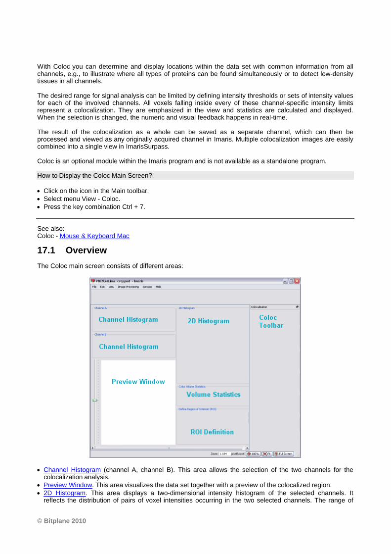
© Bitplane 2010
With Coloc you can determine and display locations within the data set with common information from allchannels, e.g., to illustrate where all types of proteins can be found simultaneously or to detect low-densitytissues in all channels.
The desired range for signal analysis can be limited by defining intensity thresholds or sets of intensity valuesfor each of the involved channels. All voxels falling inside every of these channel-specific intensity limitsrepresent a colocalization. They are emphasized in the view and statistics are calculated and displayed.When the selection is changed, the numeric and visual feedback happens in real-time.
The result of the colocalization as a whole can be saved as a separate channel, which can then beprocessed and viewed as any originally acquired channel in Imaris. Multiple colocalization images are easilycombined into a single view in ImarisSurpass.
Coloc is an optional module within the Imaris program and is not available as a standalone program.
How to Display the Coloc Main Screen?
· Click on the icon in the Main toolbar.· Select menu View - Coloc.· Press the key combination Ctrl + 7.
See also:Coloc - Mouse & Keyboard Mac
17.1 Overview
The Coloc main screen consists of different areas:
· Channel Histogram (channel A, channel B). This area allows the selection of the two channels for thecolocalization analysis.
· Preview Window. This area visualizes the data set together with a preview of the colocalized region. · 2D Histogram. This area displays a two-dimensional intensity histogram of the selected channels. It
reflects the distribution of pairs of voxel intensities occurring in the two selected channels. The range of
Imaris Reference Manual
intensity pairs considered as colocalized can be defined on the histogram.· Volume Statistics. This area displays statistics about the resulting colocalized volume. The display adapts
instantly to all modifications in the selection.· ROI Definition. This feature allows you to define a region of interest (ROI) for the entire analysis. · Coloc Toolbar. The Coloc toolbar contains several sections with all possible selection and definition tools
and settings for the histograms, the thresholding, and the display as well as the buttons for the colordefinition and the build of the Coloc channel.
17.2 Channel Histogram
This area allows the selection of the two channels for the colocalization analysis. The intensity histogramsare displayed for the currently selected channels.
Select Channel A and Channel B
The two channels for colocalization detection must be selected first.
· Select channel A and channel B from the drop-down lists. The 1D and 2D intensity histogram displays areupdated.
Adjust Threshold
· The threshold for each channel can then be defined by clicking in the histogram, dragging the colored linedirectly, or by entering the value in the threshold field.
Adjust Histogram Settings
If necessary, you can adjust in the Coloc toolbar the histogram mode and histogram options.
See also:Coloc - Coloc ToolbarColoc - Mouse & Keyboard PCColoc - Mouse & Keyboard Mac
17.3 Preview Window
This area visualizes the data set together with a preview of the colocalized region. It displays a Slicerepresentation of the data set, i.e. a 2D view from the top in the z-axis direction. On the left hand side, asliding bar with a handle allows inspecting and displaying the single slices in the data set along the z-axis.The Preview window updates in real-time the display of the colocalized region based on the actual settings ofthe colocalization parameters. The original channels can be switched on or off in the Display Adjustmentswindow.
Time Settings
There are no time-dependent parameters for the colocalization analysis. The Preview window alwaysdisplays the currently selected time point of the data set. The values in the Statistics window always refer tothe volume of the current time point. However, when the Build Coloc Channel button is pressed, the Colocchannel and statistical values for all time points are calculated.
See also:Menu Edit - Show Display AdjustmentColoc - Mouse & Keyboard PCColoc - Mouse & Keyboard Mac
© Bitplane 2010
17.4 2D Histogram
This area displays a two-dimensional intensity histogram of the selected channels. It reflects the distributionof pairs of voxel intensities occurring in the two selected channels. The range of intensity pairs considered ascolocalized can be defined on the histogram.
Adjust Channel Thresholds
Effects of the modification are instantly visible in the channel histogram A and B, and in the Preview window.
Selection Mode Threshold The channel thresholds are visible in form of a rectangle.
· Point with the cursor on the 2D histogram.· Click on the histogram to determine the thresholds. The edge of the overlaid hatched area (indicating the
selected voxel intensity range for colocalization) jumps on the marked spot.· Click on the edge and drag it to any another position in the histogram.
Selection Mode PolygonThe channel thresholds are visible as an intensity area in form of a free configurable polygon.
You draw the polygon on the 2D histogram. This method is especially useful for eliminating channel bleedthrough regions along the border of the lower intensity bins. After checking the Polygon mode, the overlaidthreshold rectangle in the 2D histogram is converted into a polygon with four corner points. You can now startto modify this polygon or to draw a completely new one. The initial point of the polygon is visible as whitefilled.
Set PointPress and hold the Shift-key. The cursor turns into a cross with a little sign. Click on the 2D histogram withthe left mouse button to place a point (vertex). Any additional point connects with lines to the initial point andthe last point inserted.
Insert Point in a LinePress and hold the Shift-key. The cursor turns into a cross with a little '' + '' sign. Point on the line betweentwo vertices and click on the line with the left mouse button to add a point.
Automatic Point SettingPress and hold the Ctrl-key. The cursor turns into a cross with a little '' + '' sign and a stack symbol. Drag thecursor around. New vertices are added automatically at each change of cursor position.
Move PointPoint on one of the vertices, click & drag the vertex around to the desired location. The polygon changes itsshape.
Move LinePoint on a line between two vertices, click & drag the line around to the desired location. The polygonchanges its shape.
Move PolygonPoint somewhere beside of the polygon edge, click & drag the polygon around to the desired location.
Delete PointShift + click on a point to delete the point.
See also:Coloc - Coloc Toolbar (selection Mode Threshold or Polygon)
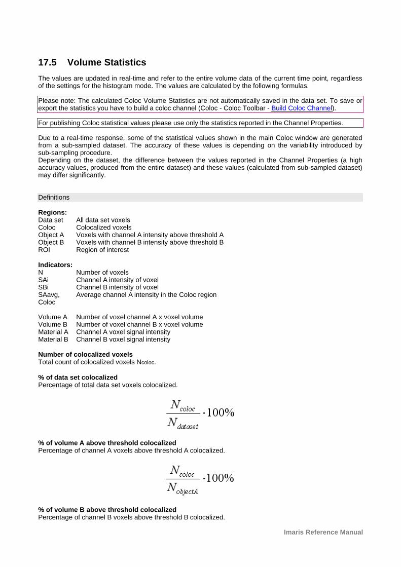
Imaris Reference Manual
17.5 Volume Statistics
The values are updated in real-time and refer to the entire volume data of the current time point, regardlessof the settings for the histogram mode. The values are calculated by the following formulas.
Please note: The calculated Coloc Volume Statistics are not automatically saved in the data set. To save orexport the statistics you have to build a coloc channel (Coloc - Coloc Toolbar - Build Coloc Channel).
For publishing Coloc statistical values please use only the statistics reported in the Channel Properties.
Due to a real-time response, some of the statistical values shown in the main Coloc window are generatedfrom a sub-sampled dataset. The accuracy of these values is depending on the variability introduced bysub-sampling procedure. Depending on the dataset, the difference between the values reported in the Channel Properties (a highaccuracy values, produced from the entire dataset) and these values (calculated from sub-sampled dataset)may differ significantly.
Definitions
Regions:Data set All data set voxelsColoc Colocalized voxelsObject A Voxels with channel A intensity above threshold AObject B Voxels with channel B intensity above threshold BROI Region of interest
Indicators:N Number of voxelsSAi Channel A intensity of voxelSBi Channel B intensity of voxelSAavg,Coloc
Average channel A intensity in the Coloc region
Volume A Number of voxel channel A x voxel volumeVolume B Number of voxel channel B x voxel volumeMaterial A Channel A voxel signal intensity Material B Channel B voxel signal intensity
Number of colocalized voxelsTotal count of colocalized voxels Ncoloc.
% of data set colocalizedPercentage of total data set voxels colocalized.
% of volume A above threshold colocalizedPercentage of channel A voxels above threshold A colocalized.
% of volume B above threshold colocalizedPercentage of channel B voxels above threshold B colocalized.
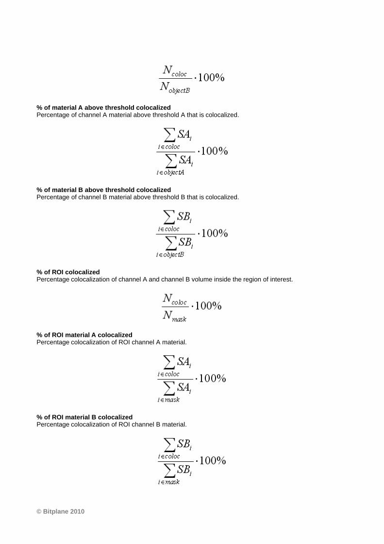
© Bitplane 2010
% of material A above threshold colocalizedPercentage of channel A material above threshold A that is colocalized.
% of material B above threshold colocalizedPercentage of channel B material above threshold B that is colocalized.
% of ROI colocalizedPercentage colocalization of channel A and channel B volume inside the region of interest.
% of ROI material A colocalizedPercentage colocalization of ROI channel A material.
% of ROI material B colocalizedPercentage colocalization of ROI channel B material.
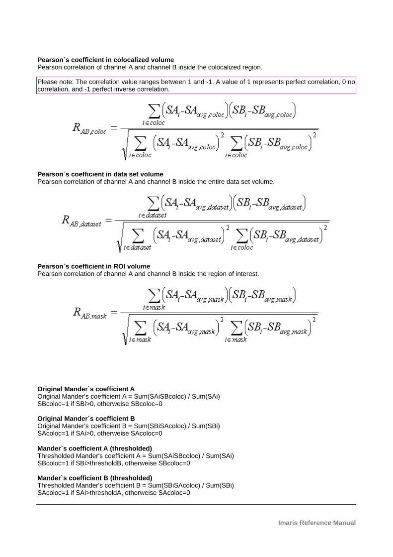
Imaris Reference Manual
Pearson`s coefficient in colocalized volumePearson correlation of channel A and channel B inside the colocalized region.
Please note: The correlation value ranges between 1 and -1. A value of 1 represents perfect correlation, 0 nocorrelation, and -1 perfect inverse correlation.
Pearson`s coefficient in data set volumePearson correlation of channel A and channel B inside the entire data set volume.
Pearson`s coefficient in ROI volumePearson correlation of channel A and channel B inside the region of interest.
Original Mander`s coefficient A Original Mander's coefficient A = Sum(SAiSBcoloc) / Sum(SAi) SBcoloc=1 if SBi>0, otherweise SBcoloc=0
Original Mander`s coefficient B Original Mander's coefficient B = Sum(SBiSAcoloc) / Sum(SBi) SAcoloc=1 if SAi>0, otherweise SAcoloc=0
Mander`s coefficient A (thresholded)Thresholded Mander's coefficient A = Sum(SAiSBcoloc) / Sum(SAi) SBcoloc=1 if SBi>thresholdB, otherweise SBcoloc=0
Mander`s coefficient B (thresholded)Thresholded Mander's coefficient B = Sum(SBiSAcoloc) / Sum(SBi) SAcoloc=1 if SAi>thresholdA, otherweise SAcoloc=0
© Bitplane 2010
See also:Menu Edit - Image Properties... - Channel 1...n - Tab Coloc Statistics (to export the statistics)Coloc - Coloc Toolbar - Build Coloc Channel (to build the coloc channel)
17.6 ROI Definition
Define Region of Interest (ROI)
This feature allows you to define a region of interest (ROI) for the entire analysis. A third channel can beselected as a masking area for the entire analysis. A masking channel is e.g. a third microscope channelacquired with settings that allows defining a region of interest by simple intensity thresholding. All voxelsoutside of the region of interest defined by the mask channel are ignored for the colocalization analysis. Thevolume excluded by the mask appears hatched in the Preview window. The mask channel is used inconjunction with the Automatic Threshold function. For this function, the selection of an appropriate region ofinterest is essential.
Mask DatasetCheck this box to activate the function.
X% of Data selectedDisplays the percentage of selected data.
Channel SelectionSelect the channel to be used from the drop-down list.
Channel Histogram Point with the cursor into the histogram and click to set the threshold. A bolded line marks the threshold inthe histogram and the corresponding value is indicated in the threshold field. The masked volume of the dataset appears hatched in the Preview window. Drag the cursor in the histogram to modify the threshold. Effectsof the modification are instantly visible in the threshold field as well as in the Preview window.
Threshold ValueEditable threshold value field.
Mask Channel and Automatic Threshold
When the mask is set as required, click the button Automatic Thresholding to calculate the thresholds.Build the colocalization channel by clicking the button Build Coloc Channel.
See also:Coloc - Coloc Toolbar - Automatic ThresholdingColoc - Coloc Toolbar - Build Coloc ChannelColoc - Mouse & Keyboard PCColoc - Mouse & Keyboard Mac
17.7 Coloc Toolbar
The Coloc toolbar contains several sections with all possible selection and definition tools and settings for thehistograms, the thresholding, and the display as well as the buttons for the color definition and the build of theColoc channel.
Selection Mode
You can define, for each of the channels separately, an intensity value as a threshold. Only voxels with anintensity value above the specified threshold will be considered for the colocalization analysis. The twothresholds are visible and can be set in four different ways:
1. As a hatched region with a bolded line on the channel histograms.2. As a value in the Threshold field of each channel (channel histogram).3. As a hatched region with bolded lines on the 2D histogram. The region always contains the top right part of
the histogram. The left and lower bolded lines define the intensity thresholds for the two channels.
Imaris Reference Manual
4. As an active contour in the Preview window.
ThresholdTo adjust the threshold value using the mouse (see above 1. and 3.), select this mode.
PolygonTo draw a polygon line in the 2D histogram (see above 4.) select this selection mode.
Automatic Thresholding
Please refer to chapter Coloc - Coloc Toolbar - Automatic Thresholding.
Histogram Mode
The histogram mode options define the voxels selection for the colocalization calculation within the data set.
Single SliceThe 2D histogram is calculated and displayed for the current slice only.
Single Time PointThe 2D histogram is calculated and shown for the entire 3D stack of the current time point. This mode allowsfor faster browsing through the data set along the z-axis.
All Time PointsThe 2D histogram is calculated and shown for an entire time data set, i.e. for all time points within the 4Ddata set.
Histogram Options
The histogram mode options are used to define the display of the 1D and 2D histograms.
Ignore Border BinsA border bin is always the first and last value in a histogram. Often a lot of voxels fall into the bin with thelowest intensity. In a frequency plot this causes a massive and unnecessary downscale of all other intensitybins which are of more interest. The border bins can therefore be ignored when scaling the display of thehistogram. Ignore is selected as default. With most data sets, checking the Ignore Border Bin andLogarithmic options allows a more representative histogram display.
LogarithmicThe frequency plot is shown in a logarithmic scaling instead of a linear scaling.
Color CodedApplies a false color look-up table to the histogram to improve the visibility of intensity differences. The highfrequencies (bins in the 2D histogram into which a lot of voxels accumulate) are shown in yellow-to-white,bins with little voxels are shown in blue-to-black.
Coloc Intensities
The Coloc intensities option defines the brightness of the calculated colocalization displayed in the Previewwindow.
Source ChannelsUses the intensities of the two channels for displaying the intensity of a colocalized voxel as the square rootof the product of the intensities of the original channels.
Constant ValueDisplays the intensity of a colocalized voxel defined by the specified value. No distinction is made whetherhigh-intensity or low-intensity voxels colocalize as long as they are within the selection.
Coloc Color
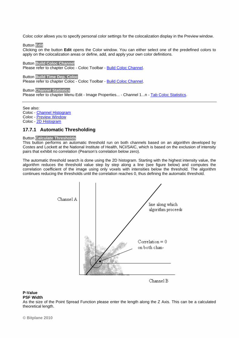
© Bitplane 2010
Coloc color allows you to specify personal color settings for the colocalization display in the Preview window.
Button EditClicking on the button Edit opens the Color window. You can either select one of the predefined colors toapply on the colocalization areas or define, add, and apply your own color definitions.
Button Build Coloc ChannelPlease refer to chapter Coloc - Coloc Toolbar - Build Coloc Channel.
Button Build Time Dep. ColocPlease refer to chapter Coloc - Coloc Toolbar - Build Coloc Channel.
Button Channel StatisticsPlease refer to chapter Menu Edit - Image Properties... - Channel 1...n - Tab Coloc Statistics.
See also:Coloc - Channel HistogramColoc - Preview WindowColoc - 2D Histogram
17.7.1 Automatic Thresholding
Button Calculate ThresholdsThis button performs an automatic threshold run on both channels based on an algorithm developed byCostes and Lockett at the National Institute of Health, NCI/SAIC, which is based on the exclusion of intensitypairs that exhibit no correlation (Pearson’s correlation below zero).
The automatic threshold search is done using the 2D histogram. Starting with the highest intensity value, thealgorithm reduces the threshold value step by step along a line (see figure below) and computes thecorrelation coefficient of the image using only voxels with intensities below the threshold. The algorithmcontinues reducing the thresholds until the correlation reaches 0, thus defining the automatic threshold.
P-ValuePSF Width As the size of the Point Spread Function please enter the length along the Z Axis. This can be a calculatedtheoretical length.
Imaris Reference Manual
Links to calculators on the WWW you can be find e.g. on the Bitplane homepage.The default in Imaris is not actually related to the PSF but only to the diagonal of the voxel size.
For more information about the P-Value and PSF Width please refer to the following publication:
Automatic and Quantitative Measurement of Protein-Protein Colocalization in Live Cells
Sylvain V. Costes,*y Dirk Daelemans,z Edward H. Cho,* Zachary Dobbin,* George Pavlakis,zand Stephen Lockett*
* Image Analysis Laboratory, National Cancer Institute, Frederick, Maryland;y National Cancer Institute/Science Applications International Corporation, Frederick, Maryland; and z Human Retrovirus Section, National Cancer Institute, Frederick, Maryland
Biophysical Journal Volume 86 June 2004 3993-4003
17.7.2 Build Coloc Channel
Button Build Coloc ChannelClicking this button calculates the colocalization channel according to the selected settings and adds it to thedata set. The channel can then be saved and is part of the data set.
Button Build Time Dep. ColocClicking this button calculates the colocalization channel according to the selected settings (calculating anautomatic threshold individually for each time point) and adds it to the data set. The channel can then besaved and is part of the data set.
Save Coloc Channel
Before the channel is added permanently to the data set it must be saved. In the menu bar select File – SaveAs or click the Save as button in the toolbar. The Save As box is displayed. Select the directory and enter thename for the file to be saved or confirm the suggestion. Select the requested file format and click OK. Thedata set is saved.
Button Channel Statistics (for the new Coloc channel)After building the Coloc channel, its statistics become available in the Image Properties. The button ChannelStatistics displays directly the Image Properties window with the statistics for the calculated channel. Thename of the channel, the description of the source channels and the selection method are indicated anddisplayed in the Image Properties on the Tab Coloc Statistics.
Export Statistics
The statistics can be exported.
Button ExportIn the Image Properties window click the Export button. The Export Coloc Statistics window is displayed.Select the directory and enter the name for the file to be saved. The statistics are saved as .csv Excel file andcan be opened directly with Microsoft Excel.
See also:Coloc - Volume Statistics
17.8 Basic Operation
The basic use of Coloc in the daily work flow comprises the following steps:
· Select the channels. · Adjust selection mode and histogram mode.
© Bitplane 2010
· Set thresholds.· Check the statistics. · Build and save the Coloc channel.
Select Channel A and Channel B
In the 1D histograms select channel A and channel B from the drop-down lists. The 1D and 2D intensityhistogram displays are updated.
Adjust Selection Mode and Histogram Mode
Before you set the thresholds, please check the appropriate parameters in the Coloc toolbar on the righthand side of the screen:
· Check as Selection Mode Threshold.· Decide, which Histogram Mode you need. Choose Single Slice for calculating the histogram for the current
slice only. Or choose Single Time Point to calculate the histogram for the entire 3D time point. Or chooseAll Time Points for the entire 4D image.
Set Thresholds
Colocalization occurs where the voxels are above threshold in channel A and channel B. You can define, foreach of the channels separately, an intensity value as a threshold. Only voxels with an intensity value abovethe specified threshold will be considered for the colocalization analysis. The two thresholds are visible andcan be set in four different ways:
1. As a hatched region with a bolded line on the channel histograms.2. As a value in the Threshold field of each channel (channel histogram).3. As a hatched region with bolded lines on the 2D histogram. The region always contains the top right part of
the histogram. The left and lower bolded lines define the intensity thresholds for the two channels.4. As an active contour in the Preview window.
A. On the 1D Channel Histogram
· Point with the cursor on the histogram. The cursor turns into a cross.· Click on the histogram to determine a threshold. The bolded left line of the overlaid hatched area
(indicating the selected voxel intensity range for colocalization) jumps on the marked spot.· Click on the line and drag it to another position in the histogram. Effects of the modification are instantly
visible in the other indications as well as in the Preview window.· Perform for both channels until the settings are as desired.
B. By Entering a Value
· Click in the Threshold field of one of the channels and enter a value, then press Enter. The bolded left lineof the overlaid hatched area (indicating the selected voxel intensity range for colocalization) jumps on themarked spot. Effects of the modification are instantly visible in the other indications as well as in thePreview display.
· Perform for both channels until the settings are as desired.
C. On the 2D Histogram
· Point with the cursor on the 2D histogram. The cursor turns into a cross.· Click on the histogram to determine the thresholds. The edge of the overlaid hatched area (indicating the
selected voxel intensity range for colocalization) jumps on the marked spot.· Click on the edge and drag it to any another position in the histogram.
D. On the Preview Window
· Click with the cursor on the image in the Preview window. An active contour is displayed, outlining imageelements brighter than the location clicked.
Imaris Reference Manual
· Drag the line on the image to define the threshold of channel A. The selection works best when startingwith brighter spots and dragging towards darker areas.
· Press and hold the Shift-key, click with the cursor on the image, then drag the line to determine thethreshold of channel B.
Check the Statistics
The statistical values are updated in real-time and refer to the entire volume data of the current time point,regardless of the settings for the histogram mode. For details please refer to chapter Coloc - VolumeStatistics.
Build Coloc Channel
Button Build Coloc ChannelClicking this button calculates the colocalization channel according to the selected settings and adds it to thedata set.
Save Coloc Channel
Before the channel is added permanently to the data set it must be saved. In the menu bar select File - SaveAs or click the Save as button in the toolbar. The Save As box is displayed. Select the directory and enter thename for the file to be saved or confirm the suggestion. Select the requested file format and click OK. Thedata set is saved.
17.8.1 Advanced Examples
The colocalization channel can be visualized like any other channel in Imaris. In the following examples, aColoc channel was built on the retina data set.
Visualize the Coloc Channel in Easy 3D
Example 1: Visualize and Adjust the Coloc Channel in Imaris Easy 3D
· After building the Coloc channel, click on the Easy 3D button in the Imaris menu bar.· Check the desired Rendering mode parameters and adjust the Settings if necessary, then click the
Calculate button. The 3D image of channel is calculated and displayed.
As the colocalized region always lays inside the initial channels, making the initial channels invisible or moretransparent allows a better view of the colocalized region.
· In the Imaris menu bar select Edit – Show Display Adjustment.· In the Display Adjustments window un-check one of the two original channels, then click the button
Calculate again. The 3D image of the original and the Coloc channel is calculated and displayed.· In the Imaris menu bar select Edit – Show Display Adjustment.· In the Display Adjustment window select the Coloc channel and adjust its settings.· In the Display Adjustment window select the remaining original channel and adjust its settings. In this
example the channel is set as partly opaque. · After each modification, click the Calculate button again to calculate the result.
Visualize the Coloc Channel in Surpass
The colocalization channel can be visualized like any other channel in Surpass.
Example 2: Create Surfaces of the Coloc Channel and Add the Two Initial Channels as Volume Rendering
· After building the Coloc channel, click on the Surpass button in the Imaris menu bar.· In the Objects toolbar click the Add New Surfaces button.· In the Surfaces Properties window check and select the Coloc channel.· Select the desired parameters. In this example, we set the threshold just below the lowest intensity values
© Bitplane 2010
in the histogram.· In the menu Surpass select Volume.· In the Imaris menu bar select Edit – Show Display Adjustment and un-check the Coloc channel. The
Surpass Volume object displays only the two initial channels. Then select the two initial channels andadjust their settings, e.g. decrease the blend opacity.
17.9 Mouse & Keyboard PC
Coloc Mouse & Keyboard Functions
Ctrl + 7 Activates the Coloc view
Selection Mode Threshold
When using one of the methods to modify the threshold values, the other indications as well as the Previewdisplay are updated in real-time.
Histogram Channel A and Histogram Channel B
Left-click on histogram Set new thresholdLeft-click on line & drag Move threshold
2D Histogram
Left-click Set channel A and channel B thresholdsLeft-click on line & drag Move channel A and channel B thresholds
Preview Window
Left-click & drag Set threshold channel AShift + left-click & drag Set threshold channel BMiddle-click & drag Move up: zoom out
Move down: zoom inShift + right-click & drag Move up: zoom out
Move down: zoom inRight-click & drag Pan image
Selection Mode Polygon
2D Histogram
Shift + left-click Add new point (any additional point connects to the last inserted point)Shift + left-click on connecting line
Insert point in a line
Shift + left-click on point
Delete point
Ctrl + left-click Add multiple new pointsLeft-click & drag (on point or line)
Move point or line
Left-click & drag (outside polygon)
Move polygon
Delete Delete single point
17.10 Mouse & Keyboard Mac
Coloc Mouse & Keyboard Functions
Command + 7 Activates the Coloc view
Imaris Reference Manual
Selection Mode Threshold
When using one of the methods to modify the threshold values, the other indications as well as the Previewdisplay are updated in real-time.
Histogram Channel A and Histogram Channel B
Click on histogram Set new thresholdClick on line & drag Move threshold
2D Histogram
Click Set channel A and channel B thresholdsClick on line & drag Move channel A and channel B thresholds
Preview Window
Click & drag Set threshold channel A Shift + click & drag Set threshold channel B
With a one-button mouse:
Shift + Ctrl + click & drag Move up: zoom outMove down: zoom in
Ctrl + click & drag Pan image
With a three-button mouse:
To configure a three button mouse on a Mac do the following:· Open the Apple-menu, select System Preferences... . · Click on the button Keyboard & Mouse.· Select the OS X mouse properties.· Change the middle button to "Button 3".
Please note: Combined mouse buttons (e.g. left + middle mouse button) do not work in Imaris.
Middle-click & drag Move up: zoom outMove down: zoom in
Right-click & drag Pan image
Selection Mode Polygon
2D Histogram
Shift + click Add new point (any additional point connects to the last inserted point)Shift + left-click on connecting line
Insert point in a line
Shift + left-click on point
Delete point
Command + click Add multiple new pointsClick & drag (on point or line)
Move point or line
Click & drag (outside polygon)
Move polygon
Delete Delete single point
© Bitplane 2010
18 Addendum
In this addendum you find the Imaris global Mouse & Keyboard PC and Mouse & Keyboard Mac functions,tips and tricks how to customize your Imaris Interface in daily routine, and a Terminology table with frequentlyused technical terms and specific image processing terms.
18.1 Mouse & Keyboard PC
In the following you find the global Mouse & Keyboard functions.
Global Mouse & Keyboard Functions
Ctrl + 1 Activates the Slice viewCtrl + 2 Activates the Section viewCtrl + 3 Activates the Gallery viewCtrl + 4 Activates the Easy 3D viewCtrl + 5 Activates the Surpass viewCtrl + 6 Activates the Key Frame AnimationCtrl + 7 Activates the Coloc viewCtrl + 8 Activates InMotion
Ctrl + A Sets zoom factor to 1 pixel per voxel and centers the image to the windowCtrl + B Adjusts zoom factor and pan position to best fit the image into the windowCtrl + C Copies current view to the clipboardCtrl + D Shows the Display Adjustment windowCtrl + E Saves Surpass scene fileCtrl + F Refreshes the textures of all viewsCtrl + I Allows to inspect and edit the image propertiesCtrl + L Opens Surpass scene fileCtrl + N Toggles display of Navigation windowCtrl + O Opens existing fileCtrl + P Allows to edit the settings of ImarisCtrl + Q Exits the applicationCtrl + R Discards all changes and opens the current data set againCtrl + S Saves the current data setCtrl + T Saves the current view as a *.tif fileCtrl + W Crops X, Y, or ZCtrl + Z Revokes the last action
Ctrl + Shift + A Adds channels of another imageCtrl + Shift + B Deletes selected channelsCtrl + Shift + C Copies the Imaris version, date and build to the clipboardCtrl + Shift + P Allows to edit figures and annotations
F1 Opens Reference ManualF2 Displays or updates the license statusF3 Automatic check for updatesF11 Maximizes the viewing area to the full size of your monitor
Ctrl + F1 Opens Quick Start Tutorials
Alt + F4 Exits the application
Del Deletes selected objects
Right-click Opens Context Sensitive Help
Global Mouse & Keyboard Functions to Navigate in All Imaris Views
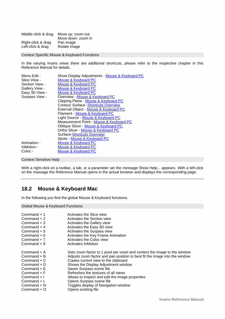
Imaris Reference Manual
Middle-click & drag Move up: zoom outMove down: zoom in
Right-click & drag Pan imageLeft-click & drag Rotate image
Context Specific Mouse & Keyboard Functions
In the varying Imaris views there are additional shortcuts, please refer to the respective chapter in thisReference Manual for details.
Menu Edit - Show Display Adjustments - Mouse & Keyboard PCSlice View - Mouse & Keyboard PCSection View - Mouse & Keyboard PCGallery View - Mouse & Keyboard PCEasy 3D View - Mouse & Keyboard PCSurpass View - Overview - Mouse & Keyboard PC Clipping Plane - Mouse & Keyboard PC
Contour Surface -Shortcuts OverviewExternal Object - Mouse & Keyboard PC
Filament - Mouse & Keyboard PCLight Source - Mouse & Keyboard PCMeasurement Point - Mouse & Keyboard PC
Oblique Slicer - Mouse & Keyboard PC Ortho Slicer - Mouse & Keyboard PC
Surface-Shortcuts Overview Spots - Mouse & Keyboard PCAnimation - Mouse & Keyboard PCInMotion - Mouse & Keyboard PCColoc - Mouse & Keyboard PC
Context Sensitive Help
With a right-click on a toolbar, a tab, or a parameter set the message Show Help... appears. With a left-clickon the massage the Reference Manual opens in the actual browser and displays the corresponding page.
18.2 Mouse & Keyboard Mac
In the following you find the global Mouse & Keyboard functions.
Global Mouse & Keyboard Functions
Command + 1 Activates the Slice viewCommand + 2 Activates the Section viewCommand + 3 Activates the Gallery viewCommand + 4 Activates the Easy 3D viewCommand + 5 Activates the Surpass viewCommand + 6 Activates the Key Frame AnimationCommand + 7 Activates the Coloc viewCommand + 8 Activates InMotion
Command + A Sets zoom factor to 1 pixel per voxel and centers the image to the windowCommand + B Adjusts zoom factor and pan position to best fit the image into the windowCommand + C Copies current view to the clipboardCommand + D Shows the Display Adjustment windowCommand + E Saves Surpass scene fileCommand + F Refreshes the textures of all viewsCommand + I Allows to inspect and edit the image propertiesCommand + L Opens Surpass scene fileCommand + N Toggles display of Navigation windowCommand + O Opens existing file
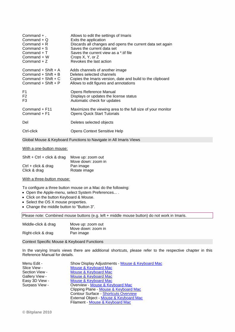
© Bitplane 2010
Command + , Allows to edit the settings of ImarisCommand + Q Exits the applicationCommand + R Discards all changes and opens the current data set againCommand + S Saves the current data setCommand + T Saves the current view as a *.tif fileCommand + W Crops X, Y, or ZCommand + Z Revokes the last action
Command + Shift + A Adds channels of another imageCommand + Shift + B Deletes selected channelsCommand + Shift + C Copies the Imaris version, date and build to the clipboardCommand + Shift + P Allows to edit figures and annotations
F1 Opens Reference ManualF2 Displays or updates the license statusF3 Automatic check for updates
Command + F11 Maximizes the viewing area to the full size of your monitorCommand + F1 Opens Quick Start Tutorials
Del Deletes selected objects
Ctrl-click Opens Context Sensitive Help
Global Mouse & Keyboard Functions to Navigate in All Imaris Views
With a one-button mouse:
Shift + Ctrl + click & drag Move up: zoom outMove down: zoom in
Ctrl + click & drag Pan imageClick & drag Rotate image
With a three-button mouse:
To configure a three button mouse on a Mac do the following:· Open the Apple-menu, select System Preferences... . · Click on the button Keyboard & Mouse.· Select the OS X mouse properties.· Change the middle button to "Button 3".
Please note: Combined mouse buttons (e.g. left + middle mouse button) do not work in Imaris.
Middle-click & drag Move up: zoom outMove down: zoom in
Right-click & drag Pan image
Context Specific Mouse & Keyboard Functions
In the varying Imaris views there are additional shortcuts, please refer to the respective chapter in thisReference Manual for details.
Menu Edit - Show Display Adjustments - Mouse & Keyboard MacSlice View - Mouse & Keyboard MacSection View - Mouse & Keyboard MacGallery View - Mouse & Keyboard MacEasy 3D View - Mouse & Keyboard MacSurpass View - Overview - Mouse & Keyboard Mac
Clipping Plane - Mouse & Keyboard Mac Contour Surface - Shortcuts Overview External Object - Mouse & Keyboard Mac Filament - Mouse & Keyboard Mac
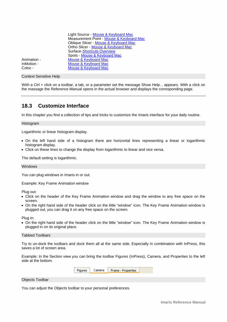
Imaris Reference Manual
Light Source - Mouse & Keyboard Mac Measurement Point - Mouse & Keyboard Mac
Oblique Slicer - Mouse & Keyboard Mac Ortho Slicer - Mouse & Keyboard Mac
Surface-Shortcuts Overview Spots - Mouse & Keyboard MacAnimation - Mouse & Keyboard MacInMotion - Mouse & Keyboard MacColoc - Mouse & Keyboard Mac
Context Sensitive Help
With a Ctrl + click on a toolbar, a tab, or a parameter set the message Show Help... appears. With a click onthe massage the Reference Manual opens in the actual browser and displays the corresponding page.
18.3 Customize Interface
In this chapter you find a collection of tips and tricks to customize the Imaris interface for your daily routine.
Histogram
Logarithmic or linear histogram display.
· On the left hand side of a histogram there are horizontal lines representing a linear or logarithmichistogram display.
· Click on these lines to change the display from logarithmic to linear and vice versa.
The default setting is logarithmic.
Windows
You can plug windows in Imaris in or out.
Example: Key Frame Animation window
Plug out:· Click on the header of the Key Frame Animation window and drag the window to any free space on the
screen.· On the right hand side of the header click on the little "window" icon. The Key Frame Animation window is
plugged out, you can drag it on any free space on the screen.
Plug in:· On the right hand side of the header click on the little "window" icon. The Key Frame Animation window is
plugged in on its original place.
Tabbed Toolbars
Try to un-dock the toolbars and dock them all at the same side. Especially in combination with InPress, thissaves a lot of screen area.
Example: In the Section view you can bring the toolbar Figures (InPress), Camera, and Properties to the leftside at the bottom.
Objects Toolbar
You can adjust the Objects toolbar to your personal preferences.
© Bitplane 2010
· Open the menu Edit - Preferences - Surpass - Object Creation Buttons to adjust your personal Objectstoolbar.
Display Mode Blend and Bland Opacity
You can select the Display Mode Blend in the Surpass view for a Volume object, in the Section view(Extended) and in the Easy 3D view. Any change in the Display Adjustment window in the parameter BlendOpacity is only visible, if a Blend Mode is selected.
18.4 Terminology
Term Description
Channel A channel is a particular piece of information that has been recorded for all voxels.Most of the time in light microscopy, the different channels are intensities that havebeen measured at different wavelengths. For instance, a two-channel data set containstwo intensities for each voxel, one intensity measured in channel 1 (e.g., green light)and one intensity in channel 2 (e.g., red light). Ideally, the intensity values present indifferent channels are independent of one another.
Coordinates Any position in the data set can be described either in the voxel grid (e.g., voxel no. 5 inx-direction) or by a coordinate, which corresponds to a m). The distance relative to adefined origin in the real world (e.g. 2 latter) requires the correct calibration of the dataset, i.e. that the voxel size is defined appropriately. Generally, in Imaris the origin of thedata set is in the left bottom corner. If the data set was cropped from a larger data set,the bottom left corner may have minimum coordinates that are not equal to (0,0,0).
Image stack A 3D data set is sometimes called an image stack consisting of 2D images stacked oneach other.
MIP A maximum intensity projection (MIP) is a computer visualization method for 3D datathat projects in the visualization plane the voxels with maximum intensity that fall in theway of parallel rays traced from the viewpoint to the plane of projection.
Original Data Set
A 3D data set that cannot be derived from any other data set using Bitplane software.Usually "Original data sets" have been acquired using an image sensor and are loadedinto Imaris.
Rendering A technique that visualizes a multi-dimensional data set as a two-dimensional imagethat can be displayed on a computer screen or printed on a laser printer.
ResultantImage
An image that has been computed using Imaris.
Standard
Deviation
In probability and statistics, the standard deviation of a probability distribution, randomvariable, or population or multiset of values is a measure of the spread of its values. Itis defined as the square root of the variance.
The standard deviation is the root mean square (RMS) deviation of values from theirarithmetic mean. For example, in the population {4, 8}, the mean is 6 and the standarddeviation is 2. This may be written: {4, 8} 6. In this case 100% of the values in thepopulation are at one standard deviation of the mean.
The standard deviation is the most common measure of statistical dispersion,measuring how widely spread the values in a data set are. If the data points are closeto the mean, then the standard deviation is small. Conversely, if many data points arefar from the mean, then the standard deviation is large. If all the data values are equal,
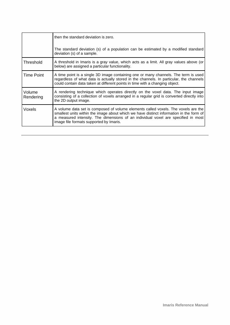
Imaris Reference Manual
then the standard deviation is zero.
The standard deviation (s) of a population can be estimated by a modified standarddeviation (s) of a sample.
Threshold A threshold in Imaris is a gray value, which acts as a limit. All gray values above (orbelow) are assigned a particular functionality.
Time Point A time point is a single 3D image containing one or many channels. The term is usedregardless of what data is actually stored in the channels. In particular, the channelscould contain data taken at different points in time with a changing object.
VolumeRendering
A rendering technique which operates directly on the voxel data. The input imageconsisting of a collection of voxels arranged in a regular grid is converted directly intothe 2D output image.
Voxels A volume data set is composed of volume elements called voxels. The voxels are thesmallest units within the image about which we have distinct information in the form ofa measured intensity. The dimensions of an individual voxel are specified in mostimage file formats supported by Imaris.