Image texture analysis for inferential sensing in the ...
198
Image texture analysis for inferential sensing in the process industries by Melissa Kistner Thesis presented in partial fulfilment of the requirements for the degree of MASTER IN ENGINEERING (Extractive Metallurgical Engineering) in the Faculty of Engineering at Stellenbosch University Supervisor Dr Lidia Auret Co-supervisor Prof. Chris Aldrich December 2013
Transcript of Image texture analysis for inferential sensing in the ...

Image texture analysis for inferential sensing
in the process industries by
Melissa Kistner
Thesis presented in partial fulfilment of the requirements for the degree
of
MASTER IN ENGINEERING (Extractive Metallurgical Engineering)
in the Faculty of Engineering at Stellenbosch University
Supervisor Dr Lidia Auret
Co-supervisor Prof. Chris Aldrich
December 2013

Stellenbosch University http://scholar.sun.ac.za

ii
Declaration By submitting this thesis electronically, I declare that the entirety of the work contained therein is my own, original work, that I am the sole author thereof (save to the extent explicitly otherwise stated), that reproduction and publication thereof by Stellenbosch University will not infringe any third party rights and that I have not previously in its entirety or in part submitted it for obtaining any qualification.
Melissa Kistner 20 September 2013 Signature Date
Copyright © 2013 Stellenbosch University All rights reserved
Stellenbosch University http://scholar.sun.ac.za

iii
Summary The measurement of key process quality variables is important for the efficient and economical operation of many chemical and mineral processing systems, as these variables can be used in process monitoring and control systems to identify and maintain optimal process conditions. However, in many engineering processes the key quality variables cannot be measured directly with standard sensors. Inferential sensing is the real-time prediction of such variables from other, measurable process variables through some form of model.
In vision-based inferential sensing, visual process data in the form of images or video frames are used as input variables to the inferential sensor. This is a suitable approach when the desired process quality variable is correlated with the visual appearance of the process. The inferential sensor model is then based on analysis of the image data.
Texture feature extraction is an image analysis approach by which the texture or spatial organisation of pixels in an image can be described. Two texture feature extraction methods, namely the use of grey-level co-occurrence matrices (GLCMs) and wavelet analysis, have predominated in applications of texture analysis to engineering processes. While these two baseline methods are still widely considered to be the best available texture analysis methods, several newer and more advanced methods have since been developed, which have properties that should theoretically provide these methods with some advantages over the baseline methods. Specifically, three advanced texture analysis methods have received much attention in recent machine vision literature, but have not yet been applied extensively to process engineering applications: steerable pyramids, textons and local binary patterns (LBPs).
The purpose of this study was to compare the use of advanced image texture analysis methods to baseline texture analysis methods for the prediction of key process quality variables in specific process engineering applications. Three case studies, in which texture is thought to play an important role, were considered: (i) the prediction of platinum grade classes from images of platinum flotation froths, (ii) the prediction of fines fraction classes from images of coal particles on a conveyor belt, and (iii) the prediction of mean particle size classes from images of hydrocyclone underflows.
Each of the five texture feature sets were used as inputs to two different classifiers (K-nearest neighbours and discriminant analysis) to predict the output variable classes for each of the three case studies mentioned above. The quality of the features extracted with each method was assessed in a structured manner, based their classification performances after the optimisation of the hyperparameters associated with each method.
In the platinum froth flotation case study, steerable pyramids and LBPs significantly outperformed the GLCM, wavelet and texton methods. In the case study of coal fines fractions, the GLCM method was significantly outperformed by all four other methods. Finally, in the hydrocyclone underflow
Stellenbosch University http://scholar.sun.ac.za

iv
case study, steerable pyramids and LBPs significantly outperformed GLCM and wavelet methods, while the result for textons was inconclusive.
Considering all of these results together, the overall conclusion was drawn that two of the three advanced texture feature extraction methods, namely steerable pyramids and LBPs, can extract feature sets of superior quality, when compared to the baseline GLCM and wavelet methods in these three case studies. The application of steerable pyramids and LBPs to further image analysis data sets is therefore recommended as a viable alternative to the traditional GLCM and wavelet texture analysis methods.
Stellenbosch University http://scholar.sun.ac.za

v
Opsomming Die meting van sleutelproseskwaliteitsveranderlikes is belangrik vir die doeltreffende en ekono-miese werking van baie chemiese– en mineraalprosesseringsisteme, aangesien hierdie verander-likes gebruik kan word in prosesmonitering– en beheerstelsels om die optimale prosestoestande te identifiseer en te handhaaf. In baie ingenieursprosesse kan die sleutelproseskwaliteits-veranderlikes egter nie direk met standaard sensors gemeet word nie. Inferensiële waarneming is die intydse voorspelling van sulke veranderlikes vanaf ander, meetbare prosesveranderlikes deur van ‘n model gebruik te maak.
In beeldgebaseerde inferensiële waarneming word visuele prosesdata, in die vorm van beelde of videogrepe, gebruik as insetveranderlikes vir die inferensiële sensor. Hierdie is ‘n gepaste benadering wanneer die verlangde proseskwaliteitsveranderlike met die visuele voorkoms van die proses gekorreleer is. Die inferensiële sensormodel word dan gebaseer op die analise van die beelddata.
Tekstuurkenmerkekstraksie is ‘n beeldanalisebenadering waarmee die tekstuur of ruimtelike organisering van die beeldelemente beskryf kan word. Twee tekstuurkenmerkekstraksiemetodes, naamlik die gebruik van grysskaalmede-aanwesigheidsmatrikse (GSMMs) en golfie-analise, is sterk verteenwoordig in ingenieursprosestoepassings van tekstuuranalise. Alhoewel hierdie twee grondlynmetodes steeds algemeen as die beste beskikbare tekstuuranalisemetodes beskou word, is daar sedertdien verskeie nuwer en meer gevorderde metodes ontwikkel, wat beskik oor eienskappe wat teoreties voordele vir hierdie metodes teenoor die grondlynmetodes behoort te verskaf. Meer spesifiek is daar drie gevorderde tekstuuranalisemetodes wat baie aandag in onlangse masjienvisieliteratuur geniet het, maar wat nog nie baie op ingenieursprosesse toegepas is nie: stuurbare piramiedes, tekstons en lokale binêre patrone (LBPs).
Die doel van hierdie studie was om die gebruik van gevorderde tekstuuranalisemetodes te vergelyk met grondlyntekstuuranaliesemetodes vir die voorspelling van sleutelproseskwaliteits-veranderlikes in spesifieke prosesingenieurstoepassings. Drie gevallestudies, waarin tekstuur ‘n belangrike rol behoort te speel, is ondersoek: (i) die voorspelling van platinumgraadklasse vanaf beelde van platinumflottasieskuime, (ii) die voorspelling van fynfraksieklasse vanaf beelde van steenkoolpartikels op ‘n vervoerband, en (iii) die voorspelling van gemiddelde partikelgrootteklasse vanaf beelde van hidrosikloon ondervloeie.
Elk van die vyf tekstuurkenmerkstelle is as insette vir twee verskillende klassifiseerders (K-naaste bure en diskriminantanalise) gebruik om die klasse van die uitsetveranderlikes te voorspeel, vir elk van die drie gevallestudies hierbo genoem. Die kwaliteit van die kenmerke wat deur elke metode ge-ekstraheer is, is op ‘n gestruktureerde manier bepaal, gebaseer op hul klassifikasieprestasie na die optimering van die hiperparameters wat verbonde is aan elke metode.
Stellenbosch University http://scholar.sun.ac.za

vi
In die platinumskuimflottasiegevallestudie het stuurbare piramiedes en LBPs betekenisvol beter as die GSMM–, golfie– en tekstonmetodes presteer. In die steenkoolfynfraksiegevallestudie het die GSMM-metode betekenisvol slegter as al vier ander metodes presteer. Laastens, in die hidrosikloon ondervloeigevallestudie het stuurbare piramiedes en LBPs betekenisvol beter as die GSMM– en golfiemetodes presteer, terwyl die resultaat vir tekstons nie beslissend was nie.
Deur al hierdie resultate gesamentlik te beskou, is die oorkoepelende gevolgtrekking gemaak dat twee van die drie gevorderde tekstuurkenmerkekstraksiemetodes, naamlik stuurbare piramiedes en LBPs, hoër kwaliteit kenmerkstelle kan ekstraheer in vergelyking met die GSMM– en golfiemetodes, vir hierdie drie gevallestudies. Die toepassing van stuurbare piramiedes en LBPs op verdere beeldanalise-datastelle word dus aanbeveel as ‘n lewensvatbare alternatief tot die tradisionele GSMM– en golfietekstuuranalisemetodes.
Stellenbosch University http://scholar.sun.ac.za

vii
Stellenbosch University http://scholar.sun.ac.za

viii
Acknowledgements On this journey, many have walked with me.
To my supervisor, Dr Lidia Auret, thank you for your sound advice, mentorship and guidance. You have inspired me with your dedication and never-ending stream of brilliant ideas from the moment that you walked in on my project. I truly appreciate the selfless effort that you have put in, over and above what would be expected, to help me make the best of this study.
To my wonderful husband, Ralf, thank you for your loving support and optimism through the ups and the downs of this journey. Thank you for being such a great sounding board, and for your optimism, patience and understanding.
Thank you to Prof. Chris Aldrich, who has gotten me interested in image analysis in the first place, and without whose encouragement and motivation I would not even have embarked on this road. Thank you for the opportunity to have learnt so much over the past two years.
To my parents, thank you for always being there for me, believing in me and encouraging me in everything that I set out to do, including this project.
Thank you to Dr Gorden Jemwa for introducing me to many of the techniques used in this work, and for guiding me through the first stretch of this journey.
To the staff and my fellow students at the Process Monitoring and Systems research group, thank you for your technical assistance and friendship.
I also express my gratitude towards the Department of Process Engineering at Stellenbosch University for their financial assistance during my post-graduate study.
Finally, I would like to thank my two cockatiels for their significant contribution of typos to this thesis by insisting that my keyboard is the perfect playground.
“Engineers like to solve problems. If there are no problems handily available, they will create their own problems.” – Scott Adams
Stellenbosch University http://scholar.sun.ac.za

ix
Table of Contents
Chapter 1 Introduction ............................................................................................... 1
1.1 Inferential sensing in the process industries..................................................................................... 2
1.2 Vision-based inferential sensing ......................................................................................................... 2 1.2.1 Framework .......................................................................................................................................... 3 1.2.2 Image analysis in the process industries ....................................................................................... 3
1.3 Texture analysis ...................................................................................................................................... 4 1.3.1 Texture feature extraction ............................................................................................................... 4 1.3.2 Classification ....................................................................................................................................... 5
1.4 Case studies ............................................................................................................................................. 6 1.4.1 Case study I: Platinum flotation froths ........................................................................................... 6 1.4.2 Case study II: Coal on a conveyor belt ............................................................................................ 7 1.4.3 Case study III: Hydrocyclone underflows ....................................................................................... 7
1.5 Objectives................................................................................................................................................. 8
1.6 Scope ........................................................................................................................................................ 8
1.7 Layout ....................................................................................................................................................... 9
Chapter 2 Vision-based inferential sensing .............................................................. 10
2.1 Introduction .......................................................................................................................................... 11
2.2 Inferential sensing ............................................................................................................................... 11 2.2.1 Inferential sensor tasks ................................................................................................................... 11 2.2.2 Inferential sensor models ............................................................................................................... 13 2.2.3 Framework ........................................................................................................................................ 13
2.3 Image analysis ....................................................................................................................................... 15 2.3.1 Machine vision ................................................................................................................................. 15 2.3.2 Image analysis for inferential sensing .......................................................................................... 17 2.3.3 Multivariate image analysis ........................................................................................................... 19
2.4 Applications in the process industries .............................................................................................. 20 2.4.1 Froth flotation .................................................................................................................................. 21 2.4.2 Rock particles on a conveyor belt ................................................................................................. 23 2.4.3 Hydrocyclones .................................................................................................................................. 24
2.5 Conclusions ........................................................................................................................................... 25
Chapter 3 Texture analysis ....................................................................................... 27
Stellenbosch University http://scholar.sun.ac.za

x
3.1 Introduction .......................................................................................................................................... 28 3.1.1 Texture modelling approaches ...................................................................................................... 28 3.1.2 Tasks in texture analysis ................................................................................................................. 29 3.1.3 Texture feature extraction ............................................................................................................. 29 3.1.4 Properties of texture analysis algorithms.................................................................................... 30
3.2 Grey-Level Co-occurrence Matrices .................................................................................................. 31 3.2.1 GLCM calculation ............................................................................................................................. 31 3.2.2 Feature extraction from GLCMs ..................................................................................................... 33 3.2.3 Applications in the process industries ......................................................................................... 34
3.3 Wavelet analysis ................................................................................................................................... 35 3.3.1 From Fourier transform to wavelet transform ............................................................................ 36 3.3.2 Continuous and discrete wavelet transform ............................................................................... 38 3.3.3 Wavelet transform of two-dimensional images .......................................................................... 40 3.3.4 Feature extraction from the wavelet representation ................................................................. 42 3.3.5 Applications in the process industries ......................................................................................... 43
3.4 Steerable pyramids .............................................................................................................................. 44 3.4.1 Filters for the steerable pyramid ................................................................................................... 45 3.4.2 Steerable pyramid decomposition ................................................................................................ 47 3.4.3 Extracting features from the steerable pyramid ........................................................................ 48 3.4.4 Applications in the process industries ......................................................................................... 50
3.5 Textons ................................................................................................................................................... 50 3.5.1 A texton algorithm .......................................................................................................................... 51 3.5.2 Filter bank for the texton algorithm ............................................................................................ 52 3.5.3 Applications in the process industries ......................................................................................... 53
3.6 Local Binary Patterns ........................................................................................................................... 53 3.6.1 Calculation of LBP features ............................................................................................................ 53 3.6.2 Alternative versions of the LBP operator ..................................................................................... 55 3.6.3 Applications in the process industries ......................................................................................... 56
3.7 Comparison between texture analysis methods ............................................................................. 57
3.8 Classification ......................................................................................................................................... 58 3.8.1 K-nearest neighbours ...................................................................................................................... 58 3.8.2 Discriminant analysis ...................................................................................................................... 59
3.9 Conclusions ........................................................................................................................................... 60
Chapter 4 Materials and methods ............................................................................. 62
4.1 Introduction .......................................................................................................................................... 63
4.2 Case studies ........................................................................................................................................... 65 4.2.1 Case study I: Platinum flotation froths ......................................................................................... 65
Stellenbosch University http://scholar.sun.ac.za

xi
4.2.2 Case study II: Coal on a conveyor belt .......................................................................................... 67 4.2.3 Case study III: Hydrocyclone underflows ..................................................................................... 69
4.3 Data partitioning, cross-validation and testing .............................................................................. 70 4.3.1 Data partitioning .............................................................................................................................. 70 4.3.2 Cross-validation ............................................................................................................................... 73 4.3.3 Testing ............................................................................................................................................... 77
4.4 Pre-processing ...................................................................................................................................... 79 4.4.1 Cropping and resizing ..................................................................................................................... 79 4.4.2 Conversion to greyscale .................................................................................................................. 80 4.4.3 Image normalisation ....................................................................................................................... 80
4.5 Dimensionality reduction ................................................................................................................... 81 4.5.1 Grey-level co-occurrence matrices ............................................................................................... 82 4.5.2 Wavelets............................................................................................................................................. 83 4.5.3 Steerable pyramids .......................................................................................................................... 83 4.5.4 Textons .............................................................................................................................................. 84 4.5.5 Local binary patterns ...................................................................................................................... 86 4.5.6 Feature set normalisation ............................................................................................................... 87 4.5.7 Principal component analysis ........................................................................................................ 87
4.6 Modelling ............................................................................................................................................... 88 4.6.1 K-nearest neighbours ...................................................................................................................... 88 4.6.2 Discriminant analysis ...................................................................................................................... 88
4.7 Performance evaluation ...................................................................................................................... 88 4.7.1 Confusion matrices .......................................................................................................................... 88 4.7.2 Sensitivity analysis .......................................................................................................................... 89
4.8 Summary ................................................................................................................................................ 90
Chapter 5 Results and discussion: Platinum flotation froths ................................... 92
5.1 Introduction .......................................................................................................................................... 93
5.2 Classification results ............................................................................................................................ 93 5.2.1 Feature extraction methods ........................................................................................................... 94 5.2.2 Classifiers .......................................................................................................................................... 96 5.2.3 Comparison between validation and test results ....................................................................... 96
5.3 Hyperparameters ................................................................................................................................. 99
5.4 LD projection ....................................................................................................................................... 100
5.5 Computer running times................................................................................................................... 105 5.5.1 Training ........................................................................................................................................... 105 5.5.2 Testing ............................................................................................................................................. 106
5.6 Conclusions ......................................................................................................................................... 106
Stellenbosch University http://scholar.sun.ac.za

xii
Chapter 6 Results and discussion: Coal on a conveyor belt .................................... 108
6.1 Introduction ........................................................................................................................................ 109
6.2 Classification results .......................................................................................................................... 109 6.2.1 Sensitivity analysis ........................................................................................................................ 111 6.2.2 Discussion ........................................................................................................................................ 111
6.3 Further analysis .................................................................................................................................. 112 6.3.1 LD projection .................................................................................................................................. 113 6.3.2 Classification results ...................................................................................................................... 116 6.3.3 Hyperparameters ........................................................................................................................... 118 6.3.4 Computer running times .............................................................................................................. 119
6.4 Conclusions ......................................................................................................................................... 121
Chapter 7 Results and discussion: Hydrocyclone underflows ................................ 122
7.1 Introduction ........................................................................................................................................ 123
7.2 Classification results .......................................................................................................................... 123 7.2.1 Sensitivity analysis ........................................................................................................................ 125 7.2.2 Discussion ........................................................................................................................................ 125
7.3 Further analysis .................................................................................................................................. 127 7.3.1 LD projection .................................................................................................................................. 127 7.3.2 Classification results ...................................................................................................................... 131 7.3.3 Optimal hyperparameters ............................................................................................................ 134 7.3.4 Computer running times .............................................................................................................. 136
7.4 Conclusions ......................................................................................................................................... 137
Chapter 8 Overall discussion and conclusions ........................................................ 138
8.1 Introduction ........................................................................................................................................ 139
8.2 Texture classification discussion and conclusions ........................................................................ 139 8.2.1 Feature extraction methods ......................................................................................................... 140 8.2.2 Classifiers ........................................................................................................................................ 142
8.3 Hyperparameter sensitivity analysis .............................................................................................. 142 8.3.1 GLCM hyperparameters ................................................................................................................ 143 8.3.2 Wavelet hyperparameters ............................................................................................................ 144 8.3.3 Steerable pyramid hyperparameters .......................................................................................... 145 8.3.4 Texton hyperparameters .............................................................................................................. 146 8.3.5 LBP hyperparameters .................................................................................................................... 147 8.3.6 Conclusion ....................................................................................................................................... 148
8.4 Research contributions and recommendations ............................................................................ 148 8.4.1 Contributions of this work ........................................................................................................... 148
Stellenbosch University http://scholar.sun.ac.za

xiii
8.4.2 Algorithm development ................................................................................................................ 149 8.4.3 Problem identification and data collection ............................................................................... 150 8.4.4 Results interpretation ................................................................................................................... 151 8.4.5 Industrial implementation ........................................................................................................... 152
8.5 Conclusions ......................................................................................................................................... 152 8.5.1 Hyperparameter optimisation ..................................................................................................... 152 8.5.2 Texture classification .................................................................................................................... 152
References ................................................................................................................... 154
Appendix A Nomenclature...................................................................................... 165
Appendix B Sample calculations ............................................................................ 169
Appendix C All repetition results: Coal on a conveyor belt ................................... 173
Appendix D All repetition results: Hydrocyclone underflows ............................... 178
Appendix E Publications based on this work ......................................................... 183
Stellenbosch University http://scholar.sun.ac.za
Chapter 1 Introduction
The measurement of key process quality variables is important for the efficient operation of many chemical and mineral processing systems. When quality variables cannot be measured directly, vision-based inferential sensing may be used to predict these variables based on the analysis of process image data.
Texture feature extraction is an image analysis approach by which the spatial information of the pixels in an image can be described. The main objective of this study is to compare the use of advanced image texture analysis methods to baseline texture analysis methods for the prediction of key process quality variables in specific process engineering applications.
Stellenbosch University http://scholar.sun.ac.za

Chapter 1 – Introduction 2
1.1 Inferential sensing in the process industries The measurement of key process quality variables is important for the efficient and profitable operation of many chemical and mineral processing systems. Since these variables are related to the quality of the process outputs, they can be used in process monitoring and control systems to identify and maintain optimal process conditions. When a process is properly monitored and controlled, it can operate at its full potential, maximising production and minimising waste and losses.
Although most modern processing plants are equipped with a large number of sensors, there are many important process variables which cannot be measured directly with standard hardware sensors. Inferential sensing is the prediction of such process variables from other, measurable process variables through some form of a model.
Inferential sensors offer the benefit of real-time variable prediction, whereas alternative measurement techniques often rely on some form of manual sampling and costly laboratory analyses, which do not provide data within a sufficient timeframe for control purposes. Also, inferential sensors do not interfere with the process at hand and may easily be incorporated in existing plant-wide control schemes. On the downside, the accuracy of predictions made by inferential sensors can be sensitive to undesirable effects that are commonly present in process data, such as measurement noise, missing values and outliers (Kadlec et al., 2009).
In many engineering processes, the desired process variable can be predicted by using an inferential sensor with process variables measured by standard sensors (such as temperature or pH) as inputs. Examples of such applications include the modelling of metal quality in a blast furnace (Radhakrishnan & Mohamed, 2000), the prediction of gas concentrations in a distillation column (Fortuna et al., 2005) and the estimation of process quality variables in a cement kiln system (Lin et al., 2007). However, in some processes there are no causal relationships between the variables that are to be predicted and the available process measurements. For example, no variables related to the particle size distribution of the ore output by a grinding process are measured with standard hardware sensors. In such cases the desired information is often related to the visual appearance of the process. One solution is then to capture image data of the process and use these data as input variables to the inferential sensor, building a model for the desired variable based on analysis of the images. The use of machine vision in such a way is termed vision-based inferential sensing in this work.
1.2 Vision-based inferential sensing Vision-based inferential sensing may be used to solve process variable prediction problems in cases where the desired process variable is correlated with the visual appearance of the process or product.
Stellenbosch University http://scholar.sun.ac.za

Chapter 1 – Introduction 3
1.2.1 Framework The framework for vision-based inferential sensing considered in this work is shown in figure 1-1, which at the most basic level consists of two steps: dimensionality reduction and modelling.
Figure 1-1: Basic vision-based inferential sensing workflow
The sensor takes image data as inputs, which are very high-dimensional as each pixel amounts to a dimension. The first step is therefore to reduce the dimensionality of the data, because modelling techniques do not perform well when the dimensionality of the input data is too high. To this end, two major types of features are typically extracted from images: spectral and textural features. Spectral features are usually extracted with multivariate image analysis (MIA), which has been very popular in recent image analysis applications in the process industries. The extraction of textural features capture the spatial organisation of images, and it is this type of feature extraction that is a main focus in this work.
The second step in vision-based inferential sensing is modelling, where the extracted features from a set of training images are used as input to train a regression or supervised classification model. Regression is used when a continuous dependent variable is to be predicted, while classification is used for the prediction of discrete dependent variable values or ranges. After the model has been trained, new, unseen images may be analysed by extracting their features and using these features as input to the trained model, allowing the model to predict the variables associated with each image.
1.2.2 Image analysis in the process industries Research on image analysis in the process industries has been focused to a large extent on MIA, a technique that was originally proposed by Geladi and others (1989) for the extraction of spectral features from images. In MIA, the usual approach is to apply principal component analysis (PCA) to an unfolded multivariate image, after which spectral features can be extracted in a number of different ways.
MIA has been applied to a diverse range of problems, such as the online grading of wood (Bharati et al., 2003), prediction of zinc grade in a sphalerite froth flotation process (Duchesne et al., 2003), estimation of the coating content of snack foods (Yu & MacGregor, 2003) and monitoring of flames in an industrial boiler (Yu & MacGregor, 2004).
Image data Dimensionality reduction Modelling Predicted variable
MIA
Texture feature extraction
Feature selection
Regression
Classification
Stellenbosch University http://scholar.sun.ac.za

Chapter 1 – Introduction 4
The extraction of spectral features is appropriate when there is a strong correlation between the predicted variable and the colour, saturation or luminosity of the image data, as in the applications mentioned here. However, in many cases the spatial organisation of pixels process images, as captured by textural features, are more descriptive of the process.
1.3 Texture analysis Texture is present in many natural images and can intuitively be interpreted by humans, but there does not yet exist a complete mathematical model that can explain the complex nature of this image property. For this reason, several types of texture analysis approaches have been developed that attempt to approximate textural properties in different ways. These approaches can be grouped into three main categories: statistical, structural and transform-based approaches. Each of these has their advantages and disadvantages, which is why most of the more recent and advanced texture analysis methods tend towards the unification of these approaches, combining their elements in various ways.
Depending on the application, the end goals of texture analysis algorithms may vary considerably. The three main problem types are texture segmentation, texture synthesis and texture classification, of which the latter is the most applicable to vision-based inferential sensing.
1.3.1 Texture feature extraction Texture classification follows the two-step procedure depicted in figure 1-1. For the texture feature extraction step, two methods have received much attention in process engineering literature: the use of grey-level co-occurrence matrices (GLCMs) and wavelet texture analysis. Even though many alternatives to these techniques exist, GLCMs and wavelets are considered as state-of-the-art texture analysis methods within the process industries (Duchesne et al., 2012).
Introduced by Haralick and others (1973), a GLCM of an image is a concise summary of the frequencies at which grey levels (pixel intensities) in an image occur at a specified displacement from each other, thus summarising the spatial relationships between pixels in an image. Statistical texture features are extracted based on one or more GLCMs of an image. There have been many process applications of GLCMs, among others in the monitoring of froth flotation processes (Bartolacci et al., 2006; Gui et al., 2013), defect detection on wooden surfaces (Conners et al., 1983; Mäenpää et al., 2003a) and quality grading of steel surfaces (Bharati et al., 2004a).
Wavelets are mathematical functions that can be convolved with images, transforming the images into representations that emphasise the frequency and spatial distribution of the image pixels, allowing for improved analysis of these properties (Mallat, 1989). Wavelet texture analysis typically involves the decomposition of images into horizontal, vertical and diagonal coefficient sets at multiple scales or levels. A feature set commonly extracted from this representation consists of the energies of all the coefficient sets. Wavelets have also seen many applications within the process industries, for example in the monitoring of flotation froth health (Liu et al., 2005; Liu & MacGregor,
Stellenbosch University http://scholar.sun.ac.za

Chapter 1 – Introduction 5
2008), defect detection in textile products (Latif-Amet et al., 2000) and tiles (Ghazvini et al., 2009), and surface quality inspection of steel surfaces (Bharati et al., 2004a; Liu et al., 2007).
While the GLCM and wavelet texture analysis methods both led to significant breakthroughs in the field of texture feature extraction when they were first popularised, newer texture analysis methods have since been developed. Specifically, three texture analysis methods have received much attention in recent texture classification literature, although they have not yet been applied extensively to process engineering applications: steerable pyramids, textons and local binary patterns (LBPs).
Steerable pyramid transformations (Simoncelli et al., 1992) are similar to wavelet transformations in that they also result in multi-resolution image representations. Steerable pyramids have the advantage of being rotation and translation invariant, a very desirable property in most image analysis applications. Furthermore, the extraction of an advanced set of statistical measurements from steerable pyramid representations has been proposed by Portilla and Simoncelli (2000).
Textons are conceptually perceived as local texture descriptors or textural “primitives” that occur frequently in images, such as blobs, edges, line terminators and line crossings (Julesz, 1981). Modern texton approaches involve image filtering and pixel clustering, with textons being defined as cluster centres in the filter response space (Leung & Malik, 2001; Varma & Zisserman, 2005). This method combines ideas from the statistical, structural and transform-based approaches in a unique way.
Finally, the LBP is a texture analysis operator for local texture characterisation, initially proposed by Olaja, Pietikäinen and Harwood (1994). The operator is applied to greyscale images in a pixel-wise fashion by comparing each pixel to its local pixel neighbourhood and employs a simple thresholding function. A major improvement to the original LBP was made when Ojala and others (2002b) proposed several mapping types that allowed for rotational invariance and proper representation of so-called “uniform” textures. The underlying principles of LBP texture analysis is the same as that of the texton algorithm, but with the advantage of reduced computational complexity.
The latter three methods described here will be referred to as advanced texture analysis methods in this work, as they combine texture analysis approaches in various ways and have some unique, desirable properties. The former two methods, GLCMs and wavelets, will be referred to as baseline methods, since their application within the process industries is already well established. There is reason to believe that the advanced texture analysis methods may be able to extract improved features when compared to the baseline methods, and this possibility is investigated in the current work.
1.3.2 Classification In the vision-based inferential sensing framework, dimensionality reduction is followed by a modelling step. In this work, two well-known and popular classification methods were considered for this step: a K-nearest neighbour (K-NN) classifier and discriminant analysis (DA). In K-nearest neighbour (K-NN) classification, given a set of training data points with known labels, a new (test)
Stellenbosch University http://scholar.sun.ac.za

Chapter 1 – Introduction 6
data point is assigned the most prevalent label among its 𝐾𝑁 closest neighbours in the feature space, with the number of neighbours 𝐾𝑁 being pre-specified.
Discriminant analysis (DA) attempts to find a weighting matrix for the training feature set that the multiplication of each feature vector with the weighting matrix results in a feature projection where the classes are maximally separated. The data are then classified according to the maximum a-posteriori probability rule.
1.4 Case studies Three vision-based inferential sensing case studies, in which textural features are expected to play a more important role than spectral features, were considered in this work:
I. the classification of platinum flotation froth images into platinum grade categories, II. the classification of coal particle images into fines fraction categories, and
III. the classification of hydrocyclone underflow images into particle size categories.
1.4.1 Case study I: Platinum flotation froths Froth flotation is a popular method for the separation of valuable metal-containing minerals from gangue minerals. The metallurgical and economic performance of a froth flotation system is determined by the grade and recovery of the valuable mineral in the froth, and ideally these key process quality variables should be measured in real-time.
Currently, the best way of measuring froth grade is with on-stream analysers (OSAs), which can provide chemical analyses of a process streams downstream of the flotation cells. However, these instruments are expensive to purchase and maintain (Liu & MacGregor, 2008), which often means that only one OSA is used to analyse the collective process stream from many flotation circuits (Holtham & Nguyen, 2002). Therefore, there could be a significant measurement delay of up to 20 minutes, and any deviations within a particular flotation circuit would be difficult to detect. This is not desirable for control purposes.
The performance of flotation systems has been linked to the visual characteristics of the froth phase (Moolman et al., 1994), and in most flotation plants the control decisions are made based on visual judgement of the appearance of the froth. For this reason, much research has been done on vision-based inferential sensing for the monitoring of flotation systems (Bonifazi et al., 2000; Duchesne et al., 2003; Gui et al., 2013).
In platinum froth flotation the colour of the froth and its grade does not appear to be correlated (Marais & Aldrich, 2011). This motivates the use of textural features as input to a classifier for platinum froth grade.
Stellenbosch University http://scholar.sun.ac.za

Chapter 1 – Introduction 7
1.4.2 Case study II: Coal on a conveyor belt The performances of many process reactors and metallurgical furnaces are influenced to a great extent by the physical properties of the feed to these processes, such as its particle size distribution. In this case study, the online prediction of the fraction of fine particles in coal on a conveyor belt is considered. The fines fraction is an important quality variable to be measured in coal feeds to gasification reactors, since excessive amounts of fine particles in the feed can impair the gas permeability of the coal bed in the reactor. This would result in non-ideal conditions for the reacting phase and, subsequently, an adverse effect on the performance of the gasifier (Aldrich et al., 2010).
Traditionally, particle size distributions or fines fractions of coal is analysed periodically via sieve analysis of belt cut samples. This method is not adequate for control purposes, due to the significant delay in the availability of information and the poor representativeness of samples, as the feed material properties can fluctuate rapidly.
The alternative of vision-based inferential sensing has been investigated using GLCM features (Aldrich et al., 2010) or texton features (Jemwa & Aldrich, 2012) as input to classifiers for fines fraction categories. The prediction of fines fraction is clearly more of a texture analysis problem than a spectral analysis problem, since groups of particles with different sizes have very distinctive textures, but their colour remains the same.
1.4.3 Case study III: Hydrocyclone underflows Hydrocyclones are used as separation devices in many engineering processes. In grinding circuits, for example, hydrocyclones take as input ore from mills and separate the particles that conform to size specifications from oversize particles. Most of the smaller, conforming particles separate into the overflow and are passed along to downstream processes, while the most of the oversize particles pass into the underflow and are returned to the mill for regrinding.
When a hydrocyclone in a grinding circuit is properly controlled, the load that circulates through the process is minimised, leading to optimal energy usage and lower operating costs (Janse van Vuuren, 2011). The operating state of a hydrocyclone can be determined visually by assessing the spray angle of the underflow (Neesse et al., 2004), and is related to the particle size distribution of the particles in the underflow (Janse van Vuuren, 2011; Uahengo, 2013).
In this work the classification of hydrocyclone underflow images into mean particle size categories is investigated. Again, particle size analysis is more suited to textural feature extraction than spectral feature extraction. In fact, colour features can be very misleading in this application, as the colour of ores can fluctuate considerably, with no relation to the mean particle size.
Stellenbosch University http://scholar.sun.ac.za

Chapter 1 – Introduction 8
1.5 Objectives The main goal of this study is to compare the use of advanced image texture analysis methods to baseline texture analysis methods for the prediction of key process quality variables in specific process engineering applications.
To achieve this goal, four secondary objectives are specified:
1. Conduct a critical survey of literature on vision-based inferential sensing and texture analysis techniques, as well as their applications within the process industries.
2. Identify and select texture analysis algorithms that, based on the literature review, have a reasonable chance of leading to the successful prediction of key process quality variables from process image data. Study and understand the theoretical concepts behind these algorithms.
3. Implement baseline and advanced texture feature extraction algorithms. Use these algorithms to extract features from process image data from three case studies where clas-ses of key process quality variables are to be predicted. Optimise the hyperparameters of all methods.
4. Assess the quality of the features extracted with each texture analysis algorithm in a structured manner by comparing their abilities to predict key process quality variable classes.
1.6 Scope The algorithms considered for implementation are limited to texture classification algorithms. That is, texture analysis algorithms are used to extract textural features from images, which are subsequently used for supervised classification of the data into two or more classes. This specifically excludes spectral feature extraction and regression from the scope of the project. The evaluation of classification performance is considered to be sufficient for the assessment of the quality of features extracted with different texture analysis algorithms, as performance trends observed from the results of classifying into ordinal classes should reasonably hold true when using regression. Since the focus is on texture feature extraction, a thorough investigation and optimisation of the classification step also falls beyond the scope of this project.
The methods explored in this study do not constitute an end product that is ready for implementa-tion in an industrial setup. Rather, this work contributes towards the long-term goal of developing effective vision-based inferential sensors for process engineering applications by assessing algorithms that may eventually be used by such sensors. An interpretation of the entire life cycle of a vision-based inferential sensing research program shows that it consists of many stages, as depicted in figure 1-2 (adapted from Wagstaff, 2012). Although all stages in such a vision-based inferential sensor research programme are discussed, the main contribution of this work is to the algorithm development or selection phase.
Stellenbosch University http://scholar.sun.ac.za

Chapter 1 – Introduction 9
1.7 Layout This thesis is organised as follows. Chapter 2 presents a literature review on vision-based inferential sensing, which is followed by a theoretical overview of five texture analysis methods in chapter 3. In chapter 4 the methodology followed in implementing and assessing the texture analysis algorithms is detailed. The results for the three case studies are presented in chapters 5, 6 and 7. Chapter 8 concludes this work with a final discussion, including the most important conclusions and recommendations for future research.
The appendices include a nomenclature (appendix A), sample calculations (appendix B), all repetition results for two of the case studies (appendices C and D) and a list of publications based on this work (appendix E).
Figure 1-2: The entire life cycle of a vision-based inferential sensor research programme.
Problem identification
Algorithm development / selection
Data collection
Results interpretation Industrial implementation
Main contribution of this work
Stellenbosch University http://scholar.sun.ac.za

Chapter 2 Vision-based inferential sensing
Inferential sensing is the use of measured process variables to predict an unknown process variable through some form of a model. Vision-based inferential sensing refers to the use of image data as input to an inferential sensor. The development of a vision-based inferential sensor consists of two main steps: dimensionality reduction and modelling. In applications of this technology in the process industries, the focus has been on multivariate image analysis (MIA). Three application areas of vision-based inferential sensing are in the monitoring of froth flotation systems, the estimation of physical properties of particulate feed materials on conveyor belts and the monitoring of hydrocyclones.
Stellenbosch University http://scholar.sun.ac.za

Chapter 2 – Vision-based inferential sensing 11
2.1 Introduction Inferential sensors can be used for the online, real-time measurement of key process quality variables, which can be very useful for monitoring and control purposes. In section 2.2, inferential sensing is discussed in detail.
In some process applications there are no causal relationships between the desired process information and the available process variables, but there is a strong relation between the desired information and the visual appearance of the process. In such cases, process images can be used as input variables to the inferential sensor and analysed to develop a model for the desired variable. The use of machine vision in this way is called vision-based inferential sensing. In applications of vision-based inferential sensing in the process industries, a strong focus has been placed on multivariate image analysis (MIA), a very well-known and efficient technique for the extraction of spectral information from images. Section 2.3 introduces image analysis and shows how this field has been applied to inferential sensing in the process industries.
Three case studies that have received considerable attention in machine vision literature will be discussed in section 2.4:
1. the monitoring of mineral froth flotation systems, 2. the characterisation of the physical properties of rock particles on conveyor belts and 3. the monitoring of hydrocyclones.
This chapter ends with conclusions in section 2.5.
2.2 Inferential sensing Inferential sensors can measure key process response or product quality variables online and in real-time, without interfering with the process at hand. In the process industries, the demand for this technology has grown over the last two decades, and there have been a large number of theoretical studies and industrial implementations. Inferential sensors are also widely known as soft sensors (Kadlec et al., 2009), virtual online analysers (Han & Lee, 2002) or observer-based sensors (Goodwin, 2000).
In many applications the desired process information can be extracted by constructing a model using the many process measurements available from standard sensors (such as pressure, pH, temperature or flow rate) as inputs. Comprehensive reviews of inferential sensing in process applications may be found in Fortuna and others (2007) and Kadlec and others (2009).
2.2.1 Inferential sensor tasks
Online prediction Inferential sensors may be used to perform a variety of tasks in process systems, the most dominant application area being the real-time estimation of key process variables that cannot be measured
Stellenbosch University http://scholar.sun.ac.za

Chapter 2 – Vision-based inferential sensing 12
within a sufficient timeframe with traditional sensors (Kadlec et al., 2009). This task will henceforth be referred to as online prediction.
Typically, the inferred variables are closely related to the efficiency of the process or quality of the product. The timeous availability of these variables can aid process operators in the accurate determination of the process state and the source of any deviations, leading to improved process control.
An example of an online prediction application of inferential sensors is the estimation of key process response variables in mineral flotation processes, such as grade or recovery. Traditionally, the froth grade is indirectly measured with on-stream analysers (OSAs), but these devices are expensive and can have significant measurement delays. In general, even if the measuring time is in the order of minutes, for instance as is the case with many on-stream gas chromatographs, the delay would still be too long if it is in a range comparable to the time constant of the process (Fortuna et al., 2007).
Automated process monitoring and control The effectiveness of manual monitoring depends largely on the experience and engineering judgement of the operator, whose task is becoming increasingly difficult as modern process plants grow in size and complexity (Venkatasubramanian et al., 2003). When the variables predicted by inferential sensors meet accuracy requirements for process control, it is relatively easy to incorporate the predicted variables into existing process monitoring and control systems. The difference between this soft sensor task and online prediction is that the variables predicted for process monitoring and control are not necessarily significant in their own regard, but rather could be any derived features that are useful inputs to a model that can determine the process state.
In some cases, new automatic control systems can be built by using variables predicted by the soft sensors as inputs. When these automatic control systems replace manual control systems, operator man-hours are reduced and the possibility of erroneous manual control actions is alleviated. This can lead to significant economical savings.
Sensor validation Another soft sensor task is sensor validation (Fortuna et al., 2007). Sensor validation is a particular type of process monitoring where the process to be monitored is another sensor. Let the sensor to be monitored be denoted by 𝜆ℎ and the inferential sensor by 𝜆𝑖. In sensor validation, the reliability of the variable measurement produced by 𝜆ℎ is determined by comparing it to the output predicted by 𝜆𝑖 (again, this task contains an online prediction component). If 𝜆ℎ is found to be defective, 𝜆𝑖 may temporarily replace the defective sensor by providing an estimate of the measured variable. Sensor validation can be used to detect and diagnose any sensor faults before a model for online prediction or automated process monitoring is built, to prevent inaccuracies in the model (Kadlec et al., 2009).
Stellenbosch University http://scholar.sun.ac.za

Chapter 2 – Vision-based inferential sensing 13
What-if analysis Inferential sensors may also be used for what-if analysis. In this type of analysis, the sensor model is used to simulate system dynamics corresponding to interesting trends in the input variables. This can lead to improved control policies and a deeper understanding of the process (Fortuna et al., 2007).
2.2.2 Inferential sensor models Soft sensors use models to relate measured process variables to unknown process response variables or product properties. The models used can be categorised into two basic types: model-driven and data-driven (Kadlec et al., 2009).
Model-driven models rely on first principle models that are derived from fundamental chemical and physical principles, for instance by using energy balances or reaction kinetics. These analytical models often focus on steady process states, and it is sometimes necessary to make simplifying assumptions during their derivation. These factors can limit their success in predicting process variables under real-life conditions.
On the other hand, data-driven models are based solely on historical process data. These models are derived empirically using statistical techniques such as regression. This is especially useful in cases where the first principle relationship between the input and output variables is not well-established, or when the analytical model is too computationally expensive for real-time implementation. It is also possible to combine the model-driven and data-driven models to form a hybrid model.
The data-based approach does have its drawbacks, particularly where low-quality input data is involved. Pre-processing of the input variables remains a difficult and time consuming task, as process data is often highly correlated, measured at different sampling rates and riddled with missing values and outliers (Kadlec et al., 2009). However, data-based models are more versatile and adaptable than their model-based counterparts. For instance, a data-based model can continue to grow and be recalibrated as more process data becomes available, so that new, unseen process states are eventually included in the model.
2.2.3 Framework The development or “training” of a data-based (empirical) inferential sensor involves a number of steps, each of which may be performed using a range of methods, as shown in figure 2-1 (adapted from Kadlec et al., 2009; Duchesne et al., 2012).
Stellenbosch University http://scholar.sun.ac.za

Chapter 2 – Vision-based inferential sensing 14
Figure 2-1: A general framework for the development of a data-based inferential sensor for online prediction. The blocks with solid frames represent required steps, while the blocks with dashed frames represent steps that may be
omitted.
Process variables
Process variable measurement
Pre-processing
Dimensionality reduction
Modelling
Desired information
Incorporation into monitoring
and control schemes
Normalisation
Outlier detection
Feature extraction
Feature selection
Regression
Key
Input / output
Algorithm step
Stellenbosch University http://scholar.sun.ac.za

Chapter 2 – Vision-based inferential sensing 15
The first step in an inferential sensing framework is to select variables from historical process data, which are usually abundantly available in modern process plants. The collection of data for the process response variable that is to be predicted can be a challenging and costly task.
The next step, pre-processing, typically includes normalisation of the variables to zero mean and unit variance, outlier detection and handling of missing data points.
Although dimensionality reduction is technically not a required step, it becomes important when a large number of input variables are used, since many of these variables are expected to be redundant or correlated. Feature extraction is one way to reduce the dimensionality of a data set, and involves transformation of the input variables to a reduced representation, for example by calculating statistical properties of the data and using these properties as features instead of the original data. With feature selection, a minimal subset of the original features is determined. One of the most well-known tools for dimensionality reduction is principal component analysis (PCA) (Pearson, 1901), which finds the orthogonal axes of maximal variation in the data and projects the data onto these axes. This allows for the variables to be represented with a smaller, transformed feature set (principal component scores), without significant loss of information.
After these data preparation steps, a regression or classification model can be trained. When the variable to be predicted is continuous, a regression model is appropriate, whereas discrete variables or categories are predicted with classification models. The various forms of regression, especially partial least squares (PLS) regression, are some of the most popular approaches for data-based inferential sensing (Wold et al., 2001).
Once the desired process response or product quality variables have been determined, these may be used to aid process operators in the determination of the process state, or optionally be incorporated into automated monitoring and control systems.
2.3 Image analysis
2.3.1 Machine vision Digital image analysis is the extraction of useful information from images by using image processing algorithms. This falls within the field of computer vision, which includes all matters related to the development of an artificial system that can interpret visual information in a meaningful way. Thus, computer vision is the larger field that also includes subjects related to image acquisition, such as lighting and imaging devices (cameras). When computer vision is used in industrial applications, it is commonly referred to as machine vision, although no universally accepted terminology exists in these overlapping fields. Hereafter, the term machine vision and not computer vision will be used, since the applications of this work are in the process industries.
Computers “see” images as data points, with each pixel in the image being a variable. In greyscale images each pixel is represented by one value called its lightness or intensity, which ranges from 0
Stellenbosch University http://scholar.sun.ac.za

Chapter 2 – Vision-based inferential sensing 16
to 255 in an 8-bit image. An example is shown in figure 2-2: the extreme intensities are black (0) and white (255), with all other intensities having values in between these two extremes.
Since each pixel is a variable, image analysis algorithms sometimes require the “unfolding” of an image: the image matrix is reshaped either row-wise or column-wise into a one-dimensional array. In the example in figure 2-2, the 7 × 11 matrix would be unfolded into a vector of length 77.
Unlike in greyscale images, pixels in multivariate images are represented by more than just one value. Colour images are often represented in the RGB colour space: each pixel is a three-dimensional variable represented by a red, green and blue value. An alternative and perhaps more intuitive colour space is the HSL system, in which a hue, saturation and lightness (intensity) value is associated with each pixel.
RGB images have three spectral bands (red, green and blue). Images represented by higher dimensional colour spaces are called multispectral images, and can include infrared spectra. These images contain additional information in the spectra that cannot be observed by the human eye, but which can be extracted with image analysis algorithms.
The goal of a machine vision implementation is usually to obtain some of the same information that would be obtained with the human visual cortex (a biological vision system). For this reason, many image analysis methods are based on models of biological vision. Although much progress has been made in the last few decades with the ever-increasing computer processing power, in most cases machines have not been able to replace human analysts. However, in some applications computers can even outperform humans, especially when a large amount of pre-processing is required.
(a) (b)
Figure 2-2: (a) An example greyscale image of an “F” with size 7 x 11 pixels, and (b) its computer representation.
0 0 0 0 0 0 0
0 120 120 120 120 0 0
0 120 255 255 255 255 0
0 120 255 0 0 0 0
0 120 255 120 0 0 0
0 120 255 255 255 0 0
0 120 255 0 0 0 0
0 120 255 0 0 0 0
0 120 255 0 0 0 0
0 0 255 0 0 0 0
0 0 0 0 0 0 0
Stellenbosch University http://scholar.sun.ac.za
Chapter 2 – Vision-based inferential sensing 17
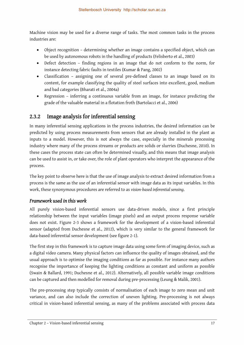
Machine vision may be used for a diverse range of tasks. The most common tasks in the process industries are:
Object recognition – determining whether an image contains a specified object, which can be used by autonomous robots in the handling of products (Felisberto et al., 2003)
Defect detection – finding regions in an image that do not conform to the norm, for instance detecting fabric faults in textiles (Kumar & Pang, 2002)
Classification – assigning one of several pre-defined classes to an image based on its content, for example classifying the quality of steel surfaces into excellent, good, medium and bad categories (Bharati et al., 2004a)
Regression – inferring a continuous variable from an image, for instance predicting the grade of the valuable material in a flotation froth (Bartolacci et al., 2006)
2.3.2 Image analysis for inferential sensing In many inferential sensing applications in the process industries, the desired information can be predicted by using process measurements from sensors that are already installed in the plant as inputs to a model. However, this is not always the case, especially in the minerals processing industry where many of the process streams or products are solids or slurries (Duchesne, 2010). In these cases the process state can often be determined visually, and this means that image analysis can be used to assist in, or take over, the role of plant operators who interpret the appearance of the process.
The key point to observe here is that the use of image analysis to extract desired information from a process is the same as the use of an inferential sensor with image data as its input variables. In this work, these synonymous procedures are referred to as vision-based inferential sensing.
Framework used in this work All purely vision-based inferential sensors use data-driven models, since a first principle relationship between the input variables (image pixels) and an output process response variable does not exist. Figure 2-3 shows a framework for the development of a vision-based inferential sensor (adapted from Duchesne et al., 2012), which is very similar to the general framework for data-based inferential sensor development (see figure 2-1).
The first step in this framework is to capture image data using some form of imaging device, such as a digital video camera. Many physical factors can influence the quality of images obtained, and the usual approach is to optimise the imaging conditions as far as possible. For instance many authors recognise the importance of keeping the lighting conditions as constant and uniform as possible (Swain & Ballard, 1991; Duchesne et al., 2012). Alternatively, all possible variable image conditions can be captured and then modelled for removal during pre-processing (Leung & Malik, 2001).
The pre-processing step typically consists of normalisation of each image to zero mean and unit variance, and can also include the correction of uneven lighting. Pre-processing is not always critical in vision-based inferential sensing, as many of the problems associated with process data
Stellenbosch University http://scholar.sun.ac.za

Chapter 2 – Vision-based inferential sensing 18
from standard sensors (such as differing sampling rates and missing measurements) are not relevant here.
Figure 2-3: A framework for the development of a vision-based inferential sensor. The blocks with solid frames represent required steps, while the blocks with dashed frames represent steps that may be omitted.
Process / product scene
Image acquisition
Pre-processing
Dimensionality reduction
Modelling
Desired information
Incorporation into monitoring
and control schemes
Normalisation
Lighting correction
MIA
Textural feature extraction
Feature selection
Regression
Classification
Key
Input / output
Algorithm step
Stellenbosch University http://scholar.sun.ac.za
Chapter 2 – Vision-based inferential sensing 19
Image data is very high-dimensional; moreover, spectral bands are usually highly correlated. Since regression or classification models do not perform well when the dimensionality of the input data is too high, dimensionality reduction is extremely important in vision-based inferential sensing. Dimensionality reduction of image data usually involves the extraction of features from the images. The problem of deciding which features to extract is the most critical part of the framework, as the overall efficiency of the sensor depends on how informative and appropriate these features are for the prediction of the desired information (Duchesne et al., 2012).
Two types of features are typically extracted: spectral and textural features. Spectral features contain information regarding the number of pixels in an image having specific colours, and do not take the spatial distribution of the colours into account. These features are commonly extracted with multivariate image analysis (MIA), which applies PCA to an unfolded multivariate image. A more detailed discussion of MIA follows in section 2.3.3.
Textural features capture the spatial organisation or texture of the pixels, but only take one spectral dimension (usually intensity) into account. Since texture analysis is a major focus area of the current work, the larger part of chapter 3 (p. 27) is dedicated to this topic.
The final step is to build a regression or classification model. Partial least squares (PLS) is a popular regression option, while common classifiers include the K-nearest neighbour (K-NN) classifier, discriminant analysis (DA) and support vector machines (SVMs). In this work, only classification case studies were considered, and the investigation of the classification step was moreover not a main focus. Therefore, only two basic and popular classifiers were considered: K-NN (detailed in chapter 3, section 3.8.1, p. 58) and DA (section 3.8.2, p. 59).
Other image analysis frameworks It should be noted that the dimensionality reduction and modelling procedure described here is not the only possible framework for the extraction of desired information from process images. Segmentation techniques have frequently been used in commercial image analysis software. For example, to determine the particle size distribution of particulate matter, segmentation techniques such as edge detection would attempt to find the edges of each particle in an image. From the segmentation of the image, mathematical correlations are used to calculate the particle size distribution. Segmentation techniques have been found to be very sensitive to irregular light reflections and shadows, which limits their robustness in industrial applications (Aldrich et al., 2012).
2.3.3 Multivariate image analysis Image analysis in the process industries has been focused on multivariate image analysis (MIA), a technique that was originally proposed by Geladi and others (1989) for the extraction of spectral features from images. The use of MIA for prediction is often referred to as multivariate image regression (MIR), which is a form of vision-based inferential sensing.
The earliest work on the application of MIA in the process industries was a conceptual study by Bharati and MacGregor (1998), who illustrated the potential of MIA for real-time process
Stellenbosch University http://scholar.sun.ac.za

Chapter 2 – Vision-based inferential sensing 20
monitoring and control by using a sequence of multispectral satellite images, since multispectral process image data were not available at the time.
There are many variations of MIA, but most techniques involve PCA of unfolded images as a primary step: for each image a PCA representation is obtained by treating the pixels as variables and the spectral bands as dimensions. Thus, each image is associated with a set of component scores (also called score images) and a set of loading vectors (the weights by which the original pixels should be multiplied to obtain the component scores).
There are several ways in which PCA results may be used to extract desired information. In the traditional approach MIA is used directly for process monitoring in a segmentation approach. Areas of interest (“masks”) are identified in the principal component space (typically a plot of the first principal component score versus the second principal component score). The pixels falling within the masks are then overlaid on the original image to assess the segmentation quality, and the procedure is repeated iteratively until a sufficient segmentation is obtained (Geladi & Grahn, 1996). This masking approach was used to detect various defects in softwood lumber, which enabled the online grading of the wood – an online prediction inferential sensor task (Bharati et al., 2003). In an application to a zinc froth flotation process, masks were used to detect clear windows on bubbles (corresponding to a deficiency in reagents) and brown spots (correlated with sphalerite grade). These were used to monitor the sphalerite grade (Duchesne et al., 2003) and to detect when the reagent dosage should be adjusted (Liu et al., 2005).
MIA may be used for prediction by computing “overall” features (based on global representations of an image) or “distribution” features (based on local regions in images). One possible set of overall features is the first loading vector of each image (from its PCA representation). This was used by Yu and MacGregor (2003) to determine snack food coating content and by Bharati and others (2004b) to predict pulp properties. Additional loading vectors may also be used: in a flotation system the mineral grade in the froth was predicted by using the first two loading vectors as input spectral features (Yang et al., 2009).
Distribution features are more appropriate when the desired information is related to local variations of spectral features within an image, and can also be more robust to variations in lighting conditions. Some successful MIA applications using distribution features include the monitoring of flames in an industrial boiler (Yu & MacGregor, 2004) and the prediction of nitrogen oxides emissions in the off-gas of a rotary cement kiln (Lin & Jørgensen, 2011).
2.4 Applications in the process industries This section gives an overview of three important application areas in the minerals processing industry, where the desired information is related to the visual appearance of the process: froth flotation systems, rock particles on conveyor belts and hydrocyclone underflows.
Stellenbosch University http://scholar.sun.ac.za

Chapter 2 – Vision-based inferential sensing 21
2.4.1 Froth flotation Flotation is a popular method for the separation of valuable metal-containing minerals from gangue material. Slurry consisting of liberated ore particles and water is conditioned through the addition of a surfactant to render the valuable mineral particles hydrophobic. The slurry is then fed to a series of flotation cells, which are aerated to introduce air bubbles. The hydrophobic particles attach to the air bubbles, which rise to the surface, forming froth. This froth then passes to the next cell and is removed from the final cell, yielding a mineral-rich concentrate.
The metallurgical and economic performance of a froth flotation system is determined by the grade and recovery of the valuable material in the concentrate. Theoretically, grade and recovery are inversely related via the specific mineral’s grade-recovery curve.
The grade (𝐺) is the ratio of the mass of valuable material reporting to the concentrate (𝑚𝐶) to the total mass of solids reporting to the concentrate (𝑀𝐶):
Recovery (𝑅) is the ratio of the mass of valuable material reporting to the concentrate (𝑚𝐶) to the mass of valuable material that was fed to the process (𝑚𝐹):
Recovery cannot be measured online, but rather has to be estimated from steady state mass balances after laboratory analysis of input ore and the final concentrate samples. Apart from the significant time delay incurred when calculating recovery in this way, some estimation error is inevitably introduced, as samples taken are not necessarily representative of entire process streams. Therefore, the usefulness of recovery as a controlled variable is limited, and most strategies focus on controlling the grade at the theoretical optimum point in the grade-recovery curve (Del Villar et al., 2010).
The mineral grade can be measured periodically via laboratory analysis, but this does not provide real-time information, as is required for process monitoring. Another possibility is the use of OSAs to measure the grade downstream from the flotation circuits, but these devices are expensive and have limited accuracy. The use of machine vision to aid in process monitoring has become an attractive alternative solution (Duchesne, 2010).
Commercial vision-based products for flotation monitoring Several commercial products have been developed for vision-based inferential sensing in flotation systems. With FrothMasterTM (developed by Outotec) properties related to the physical appearance and dynamic properties of a froth are calculated, among others the bubble size distribution, froth speed and direction, and froth stability. These measurements, together with statistical data related to these variables and grade predictions from an OSA, can be used for the automated control of the
𝐺 =
𝑚𝐶𝑀𝐶
(2-1)
𝑅 =
𝑚𝐶𝑚𝐹
(2-2)
Stellenbosch University http://scholar.sun.ac.za
Chapter 2 – Vision-based inferential sensing 22
froth speed, stability and colour. JK FrothCamTM (JK-Tech Pty. Ltd.) measures bubble size, froth structure and froth speed, which can be employed in a classification algorithm to determine variations in the process performance. VisioFroth (Metso Minerals Cisa) provides the means and standard deviations of froth speed, froth stability, bubble size distribution, colour and brightness. The product can be used to stabilise the froth speed by manipulating the level and air flow rate set points. Several other products have been developed, including PlantVisionTM (KnowledgeScape), WipFroth (WipWare), ACEFLOT (DICTUC SA) and SmartFroth (University of Cape Town).
Although most of these products have been tested in industrial environments, very few results have been reported. Also, many of these commercial solutions have been developed for specific cases and are not guaranteed to have wide applicability (Liu & MacGregor, 2008). These products mostly share two characteristics: first, they have not been developed to directly infer concentrate grade or recovery (Del Villar et al., 2010), and second, physical froth features are extracted. Although such physical features have the advantage of being intuitively interpreted and understood, it is possible that advanced texture analysis methods can extract features that contain more information than the physical features, which may improve the prediction of froth grades.
Applications of vision-based inferential sensing to flotation monitoring Several studies have shown that the concentrate grade of a froth flotation system is correlated with spectral and textural features extracted from froth images. As early as 1994, the Fast Fourier Transform (a multispectral texture analysis method) was applied to images of copper flotation froths in a study on the prediction the concentrate grade (Moolman et al., 1994). While the features extracted from froth images were discussed, quantitative predictions of concentrate grades were not made. In the same work the traditional physical features (average bubble size distribution, flow direction and bubble shape) were used to characterise different froth surface structures. A combination of colour and fractal texture features were used in a regression model to predict the grades of four different metals in a sulfide flotation system (Bonifazi et al., 2000). The grades of the four metals could be estimated with high R2 values ranging between 0.89 and 0.96. Duchesne and others (2003) used spectral features obtained with a MIA masking procedure to monitor sphalerite grade in a zinc flotation system. GLCM features were compared to spectral and physical froth features for the estimation of platinum grade in the froth (Marais & Aldrich, 2011), where an excellent R2 value of 0.99 was obtained with the best model. GLCM features combined with colour information were used to establish a qualitative relationship between the features and the grade of a bauxite flotation froth (Gui et al., 2013).
Physical features have also been used to successfully predict key flotation performance variables. Kaartinen and others (2006) measured the froth colour, bubble size distribution, froth load, froth speed and bubble collapse rate, and used the features to predict both grade and recovery in a zinc flotation system. Subsequently, a feedback control strategy was designed, with the manipulated variable being the amount of copper sulfate added. An industrial implementation of this control system led to significant financial savings due to improved zinc recoveries.
Another important task in visual flotation monitoring is termed froth health monitoring, and involves the characterisation of the quality of the froth structure. Liu and others (2005) applied multi-
Stellenbosch University http://scholar.sun.ac.za

Chapter 2 – Vision-based inferential sensing 23
resolutional multivariate image analysis (MR-MIA) to images of a zinc froth cell at the LaRonde plant of Agnico-Eagle in Quebec. Their MR-MIA approach involved the extraction of colour and texture features with principal component analysis (PCA) followed by wavelet texture analysis. Using these features, they were able to estimate froth health by calculating bubble size histograms and quantifying the visible amount of clear windows and black holes on the froth surface. Monitoring charts were developed from the PCA score plots, providing an excellent description of froth health. It has also been shown that the estimation of zinc grade can be incorporated within the MR-MIA framework. In a later study on the same flotation system (Bartolacci et al., 2006), a control scheme based on the froth description was implemented at the LaRonde plant, which resulted in a significant decrease in the occurrence of froth collapse and hence a substantially increased zinc recovery rate. Another controller was designed using the same MR-MIA features combined with additional process data, which further improved the control performance (Liu & MacGregor, 2008).
Although the merit of using physical froth features should not be discounted, it is clear from the studies described here that spectral and textural image analysis are viable alternative approaches for key performance variable prediction and froth health monitoring.
2.4.2 Rock particles on a conveyor belt Many industrial processes have as their input some type of particulate material (for example ore or coal) which is transported on conveyor belts. The physical properties of feed materials on conveyor belts are often of vital importance to the performance of downstream processes. As an example, the performance of process reactors and metallurgical furnaces can be influenced to a great extent by the particle size distribution (PSD) of the feed. Specifically, the presence of excessive amounts of fine particles (passing a 6 mm sieve mesh size) in the coal feed to fluidised bed gasification reactors can impair the gas permeability of the coal bed. This results in nonideal conditions for the reacting phases and, subsequently, an adverse effect on plant performance (Aldrich et al., 2010). The real-time availability of both PSD and ore composition measurements would be useful in crusher or semi-autogenous grinding (SAG) mill circuits to optimise power consumption, circulating load and product PSD (Duchesne, 2010).
Conventionally, PSD is analysed periodically via sieve analysis of belt cut samples, and ore composition is determined by performing laboratory analyses. These methods are not adequate for control purposes, due to the poor representativeness of samples, rapid fluctuations in feed material properties and significant measurement delays. The use of vision-based inferential sensors for online prediction of important rock feed properties is a widely investigated alternative solution.
Commercial vision-based products for monitoring of particles on conveyor belts A few vision-based commercial products have been developed for PSD analysis. The focus has been on the troubleshooting and control of crushers and grinding mills, aiming to avoid mill overload and reduce power consumption (Duchesne, 2010). Two examples are WipFrag (Wipware) and VisioRock (Metso), both of which use segmentation techniques to compute PSDs from greyscale images.
Stellenbosch University http://scholar.sun.ac.za

Chapter 2 – Vision-based inferential sensing 24
However, segmentation techniques are known to be sensitive to varying and non-uniform lighting conditions, and are prone to difficulties resulting from irregular light reflections by heterogeneous particle surfaces (Aldrich et al., 2012). The possibility has to be considered that advanced textural and spectral features can improve the quality of prediction.
Applications of vision-based inferential sensing to monitoring of particles on conveyor belts The fraction of fines in coal particles on a conveyor belt was estimated by use of GLCM texture features (Aldrich et al., 2010). The estimation of the fines fraction was treated as a classification problem by classifying images into categories of “fine”, “middling” and “coarse” using kernel-based discriminant analysis. More recently, advanced texture feature extraction methods were used to classify the same data into seven fines fraction categories (Jemwa & Aldrich, 2012).
In a different study, PSD characteristics of natural and industrial bulk aggregates were determined with a texture analysis method called the angle measure technique (Dahl & Esbensen, 2007). Ore PSDs were measured with a neural network-based inferential sensor, using “uniformity” image features as input and PSDs from WipFrag (Wipware) as initialisation of the network.
The estimation of run-of-mine ore compositions on conveyor belts is a very challenging machine vision problem, since minerals can be heterogeneous and different minerals in ores can have very similar spectral properties. Moreover, external factors such as the wetness of the ore can significantly impact the visual appearance of the ore. In a case study on a complex nickel mineral system at the Raglan Mine in Quebec, Tessier, Duchesne and Bartolacci (2007) extracted spectral features from ore images using PCA, and texture features via wavelet decomposition followed by GLCM feature extraction. It was found that excellent ore composition estimates could be made for dry ore, even though the minerals were very heterogeneous and had similar visual characteristics.
2.4.3 Hydrocyclones Hydrocyclones are separation devices used in many engineering applications, such as liquid clarification, slurry thickening and solid particle classification (Svarovsky, 1984). In the minerals processing industry, one of the most important applications of hydrocyclones is in grinding circuits, where they are used to separate particles that conform to size specifications from oversize particles that should be returned to the milling section for regrinding.
The monitoring and control of hydrocyclones in grinding circuits is important, since properly functioning hydrocyclones can significantly reduce the running costs of these circuits (Janse van Vuuren, 2011). The operating states of hydrocyclones can be determined by assessing the appearance of the underflow, and can be categorised into three types (Neesse et al., 2004):
1. dilute flow separation, where the underflow has an umbrella-like shape with low solids content,
2. dense flow separation, where the underflow has a rope-like shape with high solids content, and
3. transition state, which is a combination of the two previously mentioned states.
Stellenbosch University http://scholar.sun.ac.za

Chapter 2 – Vision-based inferential sensing 25
Although high solids content in the underflow is desired, as achieved with dense flow separation, this is not the most desirable operating state, since the conditions that lead to the rope-like shape of the underflow can cause instabilities and blocking of the hydrocyclone. The most desirable state is the transition state.
Several approaches to the measurement of process variables related to the process state have been investigated in the past. For example, a mechanical device for the measurement of the spray angle, based on contact with the underflow, has been developed by Hulbert (1993). Various types of tomography have been used to measure variables such as the underflow shape (Williams et al., 1999) and internal density distribution of the underflow (Galvin & Smitham, 1994; Gutiérrez et al., 2000). As yet, none of these techniques have been widely implemented, usually due to limiting factors such as high installation and maintenance costs or significant measurement delays.
The use of vision-based inferential sensing has also been proposed as a hydrocyclone monitoring technique. In this respect, the focus has been on extracting physical features from image data of hydrocyclone underflows, such as the:
air core size and shape (Castro et al., 1996), underflow spray angle (Petersen et al., 1996; Van Deventer et al., 2003), and underflow shape (Neesse et al., 2004; Janse van Vuuren, 2011).
The operating state of a hydrocyclone is related to the particle size distribution of the particles in the underflow: in dilute flow separation there are many fine particles, in dense flow separation there are many coarse particles, and the particle size distribution of the transition state is in-between these two extremes (Janse van Vuuren, 2011; Uahengo, 2013). Therefore, instead of attempting to use customised image analysis methods to measure features that are directly related to hydrocyclone operating states, a vision-based inferential sensor could be employed to predict the particle size distribution of the particles in the underflow. Textural features are proposed in this work as viable inputs to such a sensor, since at least to the human eye there is a strong correlation between the particle size distribution of hydrocyclone underflows and their textural properties.
2.5 Conclusions This chapter gave an overview of inferential sensing, image analysis and the fusion of the two fields, namely vision-based inferential sensing. Vision-based inferential sensors offer many benefits, such as the ability to predict variables in real-time without interfering with the process at hand. These sensors may also be incorporated into existing process monitoring and control systems with relative ease. It is therefore easy to see why there is a great desire for this technology in the process industries.
The focus of many machine vision applications in the process industries has largely been on MIA, and moreover on the extraction of spectral rather than textural image features.
Two specific vision-based inferential sensing applications, namely the monitoring of froth flotation systems and the estimation of the physical properties of particulate matter on conveyor belts, have
Stellenbosch University http://scholar.sun.ac.za

Chapter 2 – Vision-based inferential sensing 26
received much attention in machine vision literature. It was found that for both of these applications, commercial solutions often extract physical, hand-crafted features, or rely on segmentation techniques. On the other hand, several studies (usually involving MIA) have shown that the extraction of spectral and textural features is a viable alternative.
In the monitoring of hydrocyclones several vision-based monitoring approaches, using the underflow, have been proposed. As in the previous two case studies discussed, these solutions often involved the extraction of physical features that are unique to hydrocyclone underflows. The extraction of textural features is considered as a feasible alternative, since at least to the human eye there is a strong correlation between the particle size distribution of hydrocyclone underflows and their textural properties.
Stellenbosch University http://scholar.sun.ac.za

Chapter 3
Texture analysis
In this chapter a theoretical overview of five texture analysis approaches is given: grey-level co-occurrence matrices (GLCMs), wavelets, steerable pyramids, textons and local binary patterns (LBPs). Two classification methods, namely K-nearest neighbours (K-NN) and discriminant analysis (DA), are also explained. The aim here is to provide the background that is necessary to understand the methods outlined in the methodology of this work (chapter 4, page 62). Additionally, the process applications of these techniques are reviewed.
Stellenbosch University http://scholar.sun.ac.za

Chapter 3 – Texture analysis 28
3.1 Introduction Texture can be observed in many natural images, but it is difficult to find a mathematical definition of this intuitive image property. An extensive list of texture definitions was compiled by Coggins (1982), most of which are context-dependent. Rather than attempting a precise definition, in this work texture will be regarded conceptually as the spatial organisation of the pixels in an image (Rosenfeld & Kak, 1982).
In the remainder of the introduction, various background aspects around texture analysis are introduced. This is followed by the detailed description of five texture analysis methods in sections 3.2 to 3.6, with a comparison between these methods in section 3.8. The chapter ends with conclusions in section 3.9.
3.1.1 Texture modelling approaches A significant amount of information can be contained in the texture of an image. As yet, there does not exist a mathematical model that can explain the complex nature of texture, but such a model can be approximated in various ways. Several sources in literature provide a taxonomy of texture modelling approaches (see for example Tuceryan & Jain, 1998; Prats-Montalbán et al., 2011), and although terminology differs considerably, most authors agree on three basic categories:
1. statistical approaches, 2. structural approaches and 3. transform-based approaches.
Statistical texture analysis is an umbrella term for methods that involve some form of statistical modelling or feature extraction. In image analysis, the “order” of the statistical features extracted refers to the number of pixels considered together (Larabi & Charrier, 2012). Some simple examples of statistical image features are the mean and variance of the intensity histogram of an image, which are called “first-order” statistics since these do not depend on the spatial distribution of the pixels. Since textural information is not explicitly captured with these statistics, these features are limited to the description of evenly spread textures (López, 2005). Second-order statistical texture analysis methods consider the spatial relationship between pairs of pixels (two pixels at a time). A popular second-order statistical texture analysis method is the use of grey-level co-occurrence matrices (GLCMs) (Haralick et al., 1973). Other statistical approaches include autocorrelation functions (Kaizer, 1955) and various model-based approaches, such as fractal models (Peleg et al., 1984) or Markov random field models (Cohen et al., 1991).
Structural approaches to texture analysis can be traced back to early texture modelling literature, where many approaches drew inspiration from simulations of texture interpretation in the human visual system. The most influential work in this regard is probably that of Julesz, which involves the principles of pre-cognitive human texture discrimination. Julesz (1981) proposed the basic idea behind structural texture modelling: textures can be characterised by local descriptors consisting of prominent features such as blobs, line terminators and line crossings. Such texture descriptors are
Stellenbosch University http://scholar.sun.ac.za

Chapter 3 – Texture analysis 29
termed primitives or textons. A popular structural texture modelling approach is the use of mathematical morphology (Serra, 1982).
In transform-based methods some form of transform is applied to images to make their textural properties more accessible. Many of these transforms result in multi-resolutional image representations, a fact that is thought to be advantageous based on empirical evidence that textures are visually interpreted at different scales (Campbell & Robson, 1968). Examples of transform-based methods include spatial domain filtering, Fourier transforms, wavelets and steerable pyramids.
3.1.2 Tasks in texture analysis Depending on the application, the end goals of texture analysis algorithms may vary considerably. The three main problem types identified in literature are:
1. texture segmentation, 2. texture synthesis and 3. texture classification.
Texture segmentation is the partitioning of an image into regions that have homogeneous textures. Segmentation often uses feature detection methods, such as edge detection to find the separating line between the different regions. Supervised image segmentation means that some a priori information about the different segments expected in the image is available, in which case it becomes a pixel-wise classification problem. In terms of vision-based inferential sensing, the predicted variable for this task could be the percentage of the image covered by a specific region.
Texture synthesis is the development of a model for a texture and the subsequent use of this model to generate the texture. The results obtained by texture synthesis can be important visual indicators of the quality of texture representations (Portilla & Simoncelli, 2000). For example, if a synthesised texture does not appear to be visually similar to the original texture from which the model was developed, then this indicates that the texture representation was insufficient. Texture synthesis is, however, not useful for the purpose of vision-based inferential sensing.
Texture classification is the categorisation of textural images into predefined classes. This is the main focus of the current work, as it is the most useful task for vision-based inferential sensing. For example, texture classification may be used in a process monitoring application by classifying images into categories of “normal” and “deviation” process states.
3.1.3 Texture feature extraction Texture classification involves two steps: texture feature extraction followed by classification. In this chapter five texture feature extraction methods are described:
1. grey level co-occurrence matrices (GLCMs), 2. wavelets, 3. steerable pyramids, 4. textons and
Stellenbosch University http://scholar.sun.ac.za

Chapter 3 – Texture analysis 30
5. local binary patterns (LBPs).
The first two of these methods, GLCMs and wavelets, are referred to as baseline methods in this work. The last three methods are referred to as advanced methods, since they satisfy the following three criteria:
1. the method has unique characteristics and properties (see the following, section 3.1.4) that should theoretically provide some advantage over the traditional GLCMs and wavelets,
2. the method has been implemented with considerable success in recent texture analysis literature, and
3. the method has not yet been widely applied in industrial applications.
3.1.4 Properties of texture analysis algorithms
Combination of approaches The statistical, structural and transform-based approaches to texture analysis may be combined in various ways, incorporating the information obtained with each approach in a hybrid approach. It is plausible that the combination of texture analysis approaches could lead to advantages when compared to using only one approach.
Pixel neighbourhood considered The local pixel neighbourhood considered when computing textural features can play an important role in the performance of texture analysis algorithms. Texture analysis methods that incorporate appropriately sized local pixel neighbourhoods are expected to yield improved performance over methods that extract textural features on a global level only (Tuceryan & Jain, 1998).
Rotation and translation invariance When a texture analysis method is invariant to rotation and translation, it means that the features extracted from rotated or shifted versions of an image will be the same as features extracted from the original image. Although this is a highly desirable property for most applications, it is not easy to achieve (Simoncelli et al., 1992).
Multiscale representation Most natural textures occur at various scales within an image, and for this reason multi-resolution texture analysis methods, representing the same image at multiple resolutions, have been developed (Tuceryan & Jain, 1998). Multiscale representation allows for the analysis of the texture at each scale, possibly revealing textural characteristics that would have been difficult to detect when considering only local texture neighbourhoods or only global statistics of an image. Transform-based texture analysis methods are usually designed with the specific aim of multiscale representation in mind, although several other methods can be extended to account for multiscale representation to some degree.
Stellenbosch University http://scholar.sun.ac.za

Chapter 3 – Texture analysis 31
3.2 Grey-Level Co-occurrence Matrices A very well-known and established statistical method of examining texture is use of the Grey-Level Co-occurrence Matrix (GLCM), sometimes known as the grey-tone spatial-dependence matrix. Introduced by Haralick and others (1973), a GLCM of an image is a concise summary of the frequencies at which grey levels (pixel intensities) in an image occur at a specified displacement from each other, thus encapsulating the spatial relationships between pixels in an image. Statistical texture features are then extracted based on one or more GLCMs of an image.
3.2.1 GLCM calculation Natural greyscale images usually contain many grey levels, the most common being 8-bit images with 28 = 256 pixel intensities or grey levels (each grey level 𝑔 is in the range 0 ≤ 𝑔 ≤ 255, 𝑔 ∈ℕ). However, in GLCM calculation a fairly low number of grey levels (𝐺) is often used, which reduces computation time and acts as noise reduction. The greyscale image 𝐼𝐺 is therefore first scaled so that each grey level 𝑔 is scaled to lie between 0 and 1:
where 𝑔max and 𝑔min are the maximum and minimum grey levels in the original image, respectively. Then, the “image” from which the GLCM is calculated becomes:
where ⌊∙⌋ denotes the flooring operator and 𝐽 is a matrix of ones with the same dimensionality as the image. 𝐼𝐺𝐿𝐶𝑀 will have grey levels 1 ≤ 𝑔 ≤ 𝐺, 𝑔 ∈ ℕ. A popular value for 𝐺 is 8, but the hyperparameter should ideally be optimised since a trade-off exists between the benefits of noise reduction and the loss of original image information (Clausi, 2002).
Formally, the definition of the GLCM is as follows. Let us denote a GLCM of image 𝐼 as 𝑃𝐼(𝑑, 𝐺), where 𝑑 = (𝑑𝑥, 𝑑𝑦) is a chosen displacement between each pair of two pixels and 𝐺 is the number of grey levels in 𝐼𝐺𝐿𝐶𝑀. Then each entry 𝑝𝑖,𝑗 of the 𝐺 × 𝐺 sized GLCM is the number of times that the grey level pair (𝑔𝑖, 𝑔𝑗) occurs at a displacement of exactly 𝑑 apart in 𝐼𝐺𝐿𝐶𝑀. This method therefore uses pixel pairs as the pixel neighbourhood.
Figure 3-1 (a) shows an example displacement, 𝑑 = (𝑑𝑥, 𝑑𝑦) = (3,2). Also indicated on this figure are the standard directions of the 𝑥-axis and 𝑦-axis in an image, which differs from the Cartesian convention.
𝐼𝑆𝑐 =
𝐼𝐺 − 𝑔min𝑔max − 𝑔min + 1
(3-1)
𝐼𝐺𝐿𝐶𝑀 = ⌊𝐼𝑆𝑐 × 𝐺⌋ + 𝐽 (3-2)
Stellenbosch University http://scholar.sun.ac.za

Chapter 3 – Texture analysis 32
As an example of GLCM calculation, figure 3-2 shows a 5 x 5 image (with 𝐺 = 4 grey levels) on the left, with its GLCM on the right. The displacement chosen in this example is (0, 1), which means that horizontally adjacent pixel pairs are considered. Entry (1, 1) of the GLCM has a value of 1 because there is only one instance of horizontally adjacent pixels with grey levels 1 and 1. Entry (2, 1) has a value of 2 because there are two instances of horizontally adjacent pixels with grey levels 2 and 1. In a similar fashion, the entire GLCM is calculated.
Figure 3-2: [Left] A 5 x 5 image with four grey levels, and [right] its GLCM for 𝒅 = (𝟎, 𝟏)
It should be noted that in this example the ordering of grey levels in the pixel pairs was taken into account, yielding a non-symmetric matrix. However, many implementations do not take order into account, for instance there would be no differentiation between grey level pair (1, 2) and (2, 1). This would result in a symmetric co-occurrence matrix.
Figure 3-1: (a) Example of displacement 𝒅 = (𝟑, 𝟐). (b) The four directions for which GLCMs are commonly calculated.
(a) (b)
Stellenbosch University http://scholar.sun.ac.za

Chapter 3 – Texture analysis 33
As a final step, the GLCM is normalised so that the sum of its elements is equal to 1, which means that the GLCM becomes a probability matrix of joint pixel occurrences. The normalised GLCM ��𝐼 is given by:
Since the GLCM obtained is a function of 𝐺 and 𝑑, it is possible to calculate more than one GLCM for each image. The most popular choice (originally proposed by Haralick et al., 1973 and subsequently used by most studies) seems to be to fix 𝐺 and calculate GLCMs for four different displacements: (0, 𝐷), (−𝐷,𝐷), (−𝐷, 0) and (−𝐷,−𝐷), corresponding to directions 0°, 45°, 90° and 135°. 𝐷 is a hyperparameter affecting the size of the displacement 𝑑, often fixed at 𝐷 = 1. The four directions in which the GLCMs are usually calculated are depicted in figure 3-1 (b).
3.2.2 Feature extraction from GLCMs Once a set of GLCMs has been calculated, features may be extracted from them. A very well-known feature set has been proposed by Haralick and others (1973), which consists of 14 features that express the contrast, orderliness and other statistical properties of the image. However, many of these features are highly correlated among themselves (Haralick et al., 1973), which is why Haralick (1979) later reduced this set to only five features: energy (angular second moment), entropy, contrast, correlation and homogeneity (inverse difference moment). Maillard (2003) reviewed the work of many authors that have used GLCM features and concluded that these five features were overall the most popular, although all five were not always used together.
Energy and entropy are both measures of the uniformity of the GLCM. In a thorough study of feature correlations, it was found that these two features are highly correlated and that there is no need to include both features (Clausi, 2002). Excluding entropy (since this feature seems to be less popular than energy), the four features left are energy, contrast, correlation and homogeneity. These features are summarised in table 3-1. In the formulas for the features:
��𝑖,𝑗 represents the entry in row 𝑖 and column 𝑗 of the normalised GLCM ��𝐼, 𝜇𝑖 and 𝜇𝑗 are the means of the row 𝑖 and column 𝑗 of the GLCM, respectively, and 𝜎𝑖 and 𝜎𝑗 are the standard deviations of row 𝑖 and column 𝑗 of the GLCM, respectively.
After extracting these four features, each image is represented by 4 × 𝑁𝑑 features, where 𝑁𝑑 is the number of displacements considered. The standard procedure for producing a feature vector from these features is as follows. For each feature and GLCM calculated at a specified distance, the average and standard deviation across all orientations are calculated (Haralick, 1979). This ensures a degree of rotational invariance while still accounting for anisotropic effects (effects that differ according to the direction of the measurement). The length of the feature vector then becomes 4 × 2 = 8.
��𝐼 =
𝑃𝐼∑ 𝑝𝑖,𝑗𝑖,𝑗
(3-3)
Stellenbosch University http://scholar.sun.ac.za
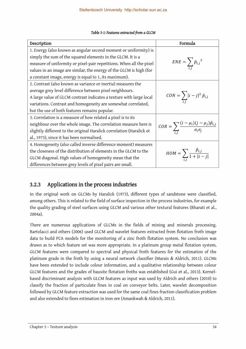
Chapter 3 – Texture analysis 34
Table 3-1: Features extracted from a GLCM
3.2.3 Applications in the process industries In the original work on GLCMs by Haralick (1973), different types of sandstone were classified, among others. This is related to the field of surface inspection in the process industries, for example the quality grading of steel surfaces using GLCM and various other textural features (Bharati et al., 2004a).
There are numerous applications of GLCMs in the fields of mining and minerals processing. Bartolacci and others (2006) used GLCM and wavelet features extracted from flotation froth image data to build PCA models for the monitoring of a zinc froth flotation system. No conclusion was drawn as to which feature set was more appropriate. In a platinum group metal flotation system, GLCM features were compared to spectral and physical froth features for the estimation of the platinum grade in the froth by using a neural network classifier (Marais & Aldrich, 2011). GLCMs have been extended to include colour information, and a qualitative relationship between colour GLCM features and the grades of bauxite flotation froths was established (Gui et al., 2013). Kernel-based discriminant analysis with GLCM features as input was used by Aldrich and others (2010) to classify the fraction of particulate fines in coal on conveyor belts. Later, wavelet decomposition followed by GLCM feature extraction was used for the same coal fines fraction classification problem and also extended to fines estimation in iron ore (Amankwah & Aldrich, 2011).
Description Formula 1. Energy (also known as angular second moment or uniformity) is simply the sum of the squared elements in the GLCM. It is a measure of uniformity or pixel-pair repetitions. When all the pixel values in an image are similar, the energy of the GLCM is high (for a constant image, energy is equal to 1, its maximum).
𝐸𝑁𝐸 =∑��𝑖,𝑗2
𝑖,𝑗
2. Contrast (also known as variance or inertia) measures the average grey level difference between pixel neighbours. A large value of GLCM contrast indicates a texture with large local variations. Contrast and homogeneity are somewhat correlated, but the use of both features remains popular.
𝐶𝑂𝑁 =∑|𝑖 − 𝑗|2 ��𝑖,𝑗𝑖,𝑗
3. Correlation is a measure of how related a pixel is to its neighbour over the whole image. The correlation measure here is slightly different to the original Haralick correlation (Haralick et al., 1973), since it has been normalised.
𝐶𝑂𝑅 =∑(𝑖 − 𝜇𝑖)(𝑗 − 𝜇𝑗)��𝑖,𝑗
𝜎𝑖𝜎𝑗𝑖,𝑗
4. Homogeneity (also called inverse difference moment) measures the closeness of the distribution of elements in the GLCM to the GLCM diagonal. High values of homogeneity mean that the differences between grey levels of pixel pairs are small.
𝐻𝑂𝑀 =∑��𝑖,𝑗
1 + |𝑖 − 𝑗|𝑖,𝑗
Stellenbosch University http://scholar.sun.ac.za

Chapter 3 – Texture analysis 35
In a very early application to defect detection for an automated lumber processing system, GLCM features combined with simple first-order statistics were used (Conners et al., 1983). Mäenpää and others (2003a) compared various texture analysis algorithms and found that GLCM features yielded the best results when applied to the detection and classification of defect types on wooden surfaces.
In the food processing industry, GLCM and wavelet features were extracted from ultrasound images of live cattle. These features were used as combined input to a regression model predicting the intramuscular fat content, which is a strong indicator of the meat grade (Kim et al., 1998). In this case the wavelet features outperformed the GLCM features. In another meat grading application, very good results were achieved by Shiranita and others (1998) using GLCMs directly as features for classification (instead of extracting Haralick texture features). Several feature sets, including GLCM features, were tested by using regression models for the prediction of important variables in the syneresis of cheese curd (Fagan et al., 2008). In this case GLCMs were among the worst of the methods that were tested.
GLCM and wavelet features are often combined or compared, and thus more studies that make use of GLCM features are discussed in the section on wavelet applications in the process industries (section 3.3.5, p. 43).
From literature reviewed here it can be concluded that GLCMs are a very popular method for texture analysis within the process industries, considering how many diverse applications of this method has been found. In most of the studies where the extraction of GLCM features was the only approach considered, the authors concluded that GLCM features were well suited to their particular application (Shiranita et al., 1998; Aldrich et al., 2010; Gui et al., 2013). However, when other features were also considered, these features have often outperformed the GLCM features (Kim et al., 1998; Fagan et al., 2008; Marais & Aldrich, 2011). This suggests that, for many applications, GLCM features may not be the optimal texture analysis method.
3.3 Wavelet analysis Research on biological vision revealed that the human visual cortex interprets visual information by performing frequency analysis, among others (Campbell & Robson, 1968). This led to the idea of applying signal processing methods, such as the well-known Fourier analysis, to images. Frequency analysis is especially suited to texture analysis, due to the spatially repetitive nature of texture, which is one of its defining properties.
Wavelet analysis (popularised by Mallat, 1989) is a signal processing method that has been developed to overcome certain limitations of Fourier analysis. Wavelets are mathematical functions that, owing to certain mathematical constraints, have a “wave-like” form. An example of a wavelet (the Daubechies 4-tap wavelet) is shown in figure 3-3.
Stellenbosch University http://scholar.sun.ac.za

Chapter 3 – Texture analysis 36
A key task in wavelet analysis is image compression, the most notable implementation being the image compression standard JPEG 2000 (Schelkens et al., 2009). In machine vision applications in the process industries, wavelet texture analysis has become a standard method (Duchesne et al., 2012). An advantage of wavelet transforms is that the set of possible prototype functions is infinite (unlike with the Fourier transform, which employs only the sine and cosine functions). It is therefore possible to optimise the wavelet algorithm for a specific application by choosing the most appropriate analysing wavelet (Materka & Strzelecki, 1998), but on the other hand this adds a hyperparameter that has to be optimised. One of the main limitations of wavelet analysis is that the representation is not rotation and translation invariant.
In section 3.3.1 the progression from the Fourier transform to the wavelet transform is explained and section 3.3.2 gives the mathematical framework for wavelet analysis. In these two sections, the various signal processing methods are explained in terms of their application to one-dimensional signals in the time-amplitude domain. However, the actual application in this work is to greyscale images, which can be seen as two-dimensional “signals” in a spatial-spatial-intensity domain. The application of wavelet analysis to images is detailed in section 0, and the features that may be extracted from the wavelet representation of an image are discussed in section 3.3.4. Section 3.3.5 concludes with applications of wavelet analysis in the process industries.
3.3.1 From Fourier transform to wavelet transform
Fourier transform The Fourier transform (FT) is a mathematical transformation that is used to represent time-amplitude domain signals in the frequency-amplitude domain. The FT is suitable for the analysis of stationary signals (in which the frequency components remain the same at all times), but its effectiveness is limited in the analysis of non-stationary signals, since all information regarding the times at which certain frequencies occur is lost.
Figure 3-3: The Daubechies 4-tap wavelet computed with
10 iterations
Stellenbosch University http://scholar.sun.ac.za

Chapter 3 – Texture analysis 37
Short-time Fourier transform Most real-life signals (including most natural images) are non-stationary. In an attempt to overcome the limitation of the FT, the short-time Fourier transform (STFT) was developed (Gabor, 1946; Allen & Rabiner, 1977). The main principle behind the STFT is to divide the signal into segments or “windows” along the time axis and then determine the frequency components that exist within each window separately. For each window, this is done by multiplying the signal to be transformed with a compactly supported window function (which is zero-valued outside the window) before applying the FT. The window function is a function of translation (𝜏), which is directly related to time (𝑡), as it indicates where along the time axis the window function is located (where it has non-zero values).
The result after applying the STFT is a representation of the signal in three dimensions (time, frequency and amplitude). However, in this representation neither the time nor the frequency information is exact, a problem which is rooted in Heisenberg’s uncertainty principle. In the context of signal processing, Heisenberg’s principle states that it is not possible to determine the exact frequency components that exist at a given instant in time. This leads to the so-called “resolution problem” of signal processing: there exists a trade-off between the resolution (precision or exactness) of the time information and the resolution of the frequency information. One can obtain a very good time resolution by using very narrow window functions, so that the interval of time considered approaches an instant, but this will give poor frequency resolution (the exact frequency components will not be known). By using wider window functions, a better frequency resolution can be obtained, but the time resolution will become worse (only the frequency components occurring during a longer interval of time will be known). When increasing the width of the window to the entire duration of the signal, the normal FT is obtained, with perfect frequency resolution but zero time resolution.
Wavelet transform The wavelet transform (WT) was developed to sidestep the resolution problem of the STFT by maintaining a high time resolution (and thus low frequency resolution) at high frequencies, and a high frequency resolution (but low time resolution) at low frequencies. This is done by altering the size of the wavelet, which is the “window function” used in wavelet analysis, through dilation or contraction. Varying the time-frequency resolution in this way is well-suited to the analysis of most natural signals, since high frequencies often occur for short periods of time, while low frequencies tend to be present for the entire duration of the signal. The concept of multi-resolution analysis is illustrated in figure 3-4.
Stellenbosch University http://scholar.sun.ac.za

Chapter 3 – Texture analysis 38
Figure 3-4: The varying time-frequency resolutions used in the WT
In figure 3-4, each rectangular shape corresponds to a single value (amplitude) of the WT in the time-frequency domain, and has a fixed non-zero area. At lower frequencies, the heights of the rectangular shapes are smaller, which corresponds to better frequency resolutions (since there is less uncertainty regarding the exact frequency values). In turn, the widths of the rectangular shapes are larger at lower frequencies, corresponding to poorer time resolutions. The exact opposite is seen at high frequencies: the larger heights indicate poorer frequency resolutions and the smaller widths indicate better time resolutions. If the STFT was to be illustrated in the same manner, the plot would have consisted of squares with the same area as the rectangles in figure 3-4, due to the constant width of the window function.
Both the STFT and WT result in representations in the three-dimensional time-frequency-amplitude domain, or equivalently translation-frequency-amplitude domain (time corresponds linearly to translation) However, the WT is usually shown in the translation-scale-amplitude domain, where scale (𝑠) is the reciprocal of frequency (𝑓):
3.3.2 Continuous and discrete wavelet transform
Continuous wavelet transform The continuous wavelet transform (popularised by Meyer, 1986) is formally given as:
𝑠 =
1
𝑓 (3-4)
𝑊(𝑠, 𝜏) = ∫𝑥(𝑡)𝜓𝑠,𝜏
∗ (𝑡)𝑑𝑡 (3-5)
Stellenbosch University http://scholar.sun.ac.za

Chapter 3 – Texture analysis 39
This equation shows how 𝑥(𝑡), a signal in the time domain, is transformed into function 𝑊(𝑠, 𝜏) by multiplying it with the wavelet 𝜓𝑠,𝜏(𝑡) and then integrating over all times. The asterisk in the term 𝜓𝑠,𝜏∗ means that conjugate transpose of 𝜓𝑠,𝜏 is used. By applying the transform, 𝑥(𝑡) is represented
in the translation (𝜏)-scale (𝑠)-amplitude domain. To perform the multi-resolution analysis, different wavelets for this decomposition are generated from a single prototype function or “mother wavelet” (𝜓) by using different scales and translations:
To allow for the computer computation of the continuous WT, the transformation has to be discretised. For the continuous WT this is done by sampling the translation-scale plane at a uniform sampling rate, but although the transformation then technically becomes discrete, this is still known as the continuous WT.
Discrete wavelet transform If the wavelet used in the transform satisfies certain mathematical conditions, it is possible to decrease the sampling rate of the scale without losing any information. The discrete wavelet transform (Croisier et al., 1976) is obtained by sampling the scale at a non-uniform sampling rate. Formally, discrete dilated and contracted wavelets are generated according to:
In (3-7), 𝑠0 is the constant scaling factor, and is typically chosen as 𝑠0 = 2. The constant translation factor is usually chosen as 𝜏0 = 1. The new scale and translation of the discrete wavelet are 𝑠0
𝑗 and 𝑘𝜏0 , respectively. 𝑗 = {1, 2, 3,… , 𝐽max} is the level of decomposition, where 𝐽max is a certain maximum level at which the scale becomes too large (frequency becomes too small) to analyse. This means that for 𝑠0 = 2 the scale is discretised on a logarithmic grid with base 2, so that only the wavelets at scales {2, 4, 8, 16,… } are used for transformation. The translation is sampled according to the sampling rate of the scale axis, so in this case the translation sampling rate is reduced by a factor of 2 as scale increases, for example 𝑘 = {64, 32, 16, 8, … }.
The discrete wavelet transform is defined in the same way as the continuous wavelet transform, but using discrete wavelets 𝜓𝑗,𝑘(𝑡) instead of continuous wavelets 𝜓𝑠,𝜏(𝑡):
From the mother wavelet 𝜓(𝑡), a sequence of scaling coefficients 𝑤 for that wavelet can be calculated to allow for the efficient computation of the WT, which is explained in more detail in section 0. The scaling coefficient set 𝑤 is finite if the mother wavelet is compactly supported (exactly zero outside a small interval), and major breakthrough for wavelets came with the advent
𝜓𝑠,𝜏(𝑡) =
1
√𝑠𝜓 (𝑡 − 𝜏
𝑠) (3-6)
𝜓𝑗,𝑘(𝑡) =
1
√𝑠0𝑗
𝜓(𝑡 − 𝑘𝜏0𝑠0
𝑗
𝑠0𝑗
) (3-7)
𝑊(𝑗, 𝑘) = ∫𝑥(𝑡)𝜓𝑗,𝑘
∗ (𝑡)𝑑𝑡 (3-8)
Stellenbosch University http://scholar.sun.ac.za

Chapter 3 – Texture analysis 40
of such compactly supported wavelets (Daubechies, 1988). The scaling coefficient set may be thought of as a filter and is often called a scaling filter.
3.3.3 Wavelet transform of two-dimensional images The signal processing methods in the previous two subsections were explained in terms of their application to one-dimensional signals in the time-amplitude domain. Wavelet analysis can easily be extended to two-dimensional signals, where the vertical and horizontal spatial positions in the image correspond to “time” in a conventional signal, and the greyscale intensity corresponds to “amplitude” in a conventional signal. Images are thus “signals” in the spatial-spatial-intensity domain.
Due to the mathematical properties of the discrete wavelet transform it can be applied to an image at level 𝑗 by using only the scaling filter 𝑤 and the filter response at the previous level (𝑐𝐴𝑗−1). This leads to a considerable saving in computation time and complexity. The procedure for discrete wavelet decomposition as developed by Daubechies (1988), specifically as applied to two-dimensional greyscale images, is described in this section.
Figure 3-5 shows the 𝑗th level two-dimensional discrete wavelet decomposition of an image. The algorithm is initialised by setting 𝑐𝐴0 as the original image. From the scaling filter 𝑤 a lowpass filter 𝑤𝐿 and highpass filter 𝑤𝐻 is constructed.
In the remainder of the algorithm, the image is convolved with the lowpass and highpass filters and downsampled. If an image 𝐼 is convolved with any filter 𝜔, the convolutional output 𝑐 has the same dimensions as 𝐼. An element in the convolutional output, 𝑐(𝑥𝑝, 𝑥𝑞), is defined as:
𝑐(𝑥𝑝, 𝑥𝑞) = ∑ ∑ 𝐼(𝑖, 𝑗) × 𝜔(𝑥𝑝 − 𝑖, 𝑥𝑞 − 𝑗)
∞
𝑗=−∞
∞
𝑖=−∞
(3-9)
Stellenbosch University http://scholar.sun.ac.za

Chapter 3 – Texture analysis 41
Let us consider the calculation of the level 𝑗 horizontal approximation image or “coefficients” 𝑐𝐻𝑗 to illustrate the procedure shown in figure 3-5. First, the approximation coefficients 𝑐𝐴𝑗−1 are convolved with the lowpass filter 𝑤𝐿 in a row-wise manner. The result is then downsampled by keeping the evenly indexed columns (as represented in figure 3-5 by a circle containing a “2” and a downward arrow). Then, the downsampled result is convolved column-wise with the highpass filter 𝑤𝐻, after which the rows are downsampled by retaining the evenly indexed rows. The result is the horizontal approximation coefficients 𝑐𝐻𝑗.
At each level 𝑗 the approximation image 𝑐𝐴𝑗−1 is decomposed into four sets of coefficients: the approximation coefficients 𝑐𝐴𝑗 and the horizontal, vertical and diagonal detail coefficients (𝑐𝐻𝑗, 𝑐𝑉𝑗 and 𝑐𝐷𝑗). To proceed with decomposition at level 𝑗 + 1, the same procedure is applied to 𝑐𝐴𝑗. It is also possible to proceed to the next level by further decomposing all four approximation and detail images, a method that is called wavelet packet analysis. However, this quickly leads to a very high dimensionality when 𝑗 > 2, so the former approach is usually preferred. An example of a wavelet representation is shown in figure 3-6.
Figure 3-5: Discrete two-dimensional wavelet decomposition at level j. 𝒄𝑨, 𝒄𝑯, 𝒄𝑽 and 𝒄𝑫 refer to approximation and detail coefficients. 𝒘𝑳 and 𝒘𝑯 refer to the highpass and lowpass filters, respectively. The circles containing “2” and a
downward arrow indicate downsampling of the coefficients by retaining only every other row or column.
Stellenbosch University http://scholar.sun.ac.za

Stellenbosch University http://scholar.sun.ac.za

Chapter 3 – Texture analysis 43
extraction, the only difference being that the GLCM energy is normalised. Due to special mathematical properties, energy is conserved in wavelet decomposition. This means that the sum of the energies of all detail coefficient sets and the final approximation coefficient set is equal to the energy of the original image.
The energy features are concatenated into a vector which is commonly called the wavelet energy signature. Some authors calculate the energy of all the detail images (each direction at each level) plus the final approximation image, giving a feature vector of length 3𝐽 + 1. However, the final approximation image often captures variations due to inconsistent lighting, and therefore it may be better to use only detail coefficients (Bharati et al., 2004a).
Several authors have combined wavelets and GLCMs by calculating GLCMs of approximation and detail coefficients at different levels, and subsequently extracting subsets of the popular Haralick features.
3.3.5 Applications in the process industries There have been several implementations of wavelets in the minerals processing and mining industries. Liu and others (2005) successfully monitored froth health in a zinc flotation system by using MR-MIA: first PCA was applied on images and then score images were decomposed using a wavelet transformation. In a follow-up article, even better results were achieved by sampling the wavelet transform at an even scale instead of a dyadic scale (Liu & MacGregor, 2008). GLCM and wavelet features were compared for the estimation of run-of-mine ore compositions (Tessier et al., 2007); in this case the use of wavelet features yielded superior results. In another application to particulate matter on conveyor belts, wavelet decomposition followed by GLCM feature extraction was used to classify the fraction of fines in coal and iron ore (Amankwah & Aldrich, 2011).
Wavelets have been widely used for defect detection. The presence of defects in textile products were determined using features extracted from the GLCMs of wavelet image representations (Latif-Amet et al., 2000). Statistical features extracted from wavelet detail coefficients were used in a neural network classifier that could detect defects in tiles (Ghazvini et al., 2009). In another tile defect detection problem, Fathi and others (2012) applied a wavelet transformation followed by GLCM calculation to extract features for a neural network. Cord and others (2010) employed higher-order types of wavelets called curvelets, as well as morphological feature extraction, to detect scratches on steel surfaces.
In the microelectronics industry, Lin (2007) used wavelet texture analysis for the detection of ripple defects on surfaces of ceramic capacitors. Wavelet features formed the basis of a hidden Markov tree model for the detection and classification of surface defects on memory device wafers (Chen et al., 2009).
Surface quality inspection is another field where wavelets are popular. Rolled steel sheets were classified with discriminant analysis into various quality grades by using GLCM features, energies of wavelet approximation images and other statistical features (Bharati et al., 2004a). Wavelet texture analysis yielded the best results. In later work on the same steel quality grading problem, a
Stellenbosch University http://scholar.sun.ac.za

Chapter 3 – Texture analysis 44
variation called the wavelet packet transform was used and the optimal decomposition level was determined. These changes improved the classification performance (Liu et al., 2007). By adding additional feature selection and feature reduction steps to the algorithm, even further improved classification results were obtained (Kim et al., 2009).
Other surface grading applications include the grading of various fabrics according to the degree of pilling (Zhang et al., 2007) and paper quality grading for use in an online, real-time monitoring system for a paper formation process (Reis & Bauer, 2009). Wavelet texture analysis followed by PCA dimensionality reduction was used to build a latent variable space model for the grading and monitoring of the aesthetic quality of engineered stone countertops (Liu & MacGregor, 2006).
Other miscellaneous process applications include:
categorisation of different corrosion types in various materials (Livens et al., 1996), prediction of dispersion in the mixing of polymer powders, where GLCM and wavelet
features were shown to outperform traditional measures used to characterise such mixing processes (Gosselin et al., 2008),
prediction of mechanical properties of polymer blend films, such as toughness and tensile strength, with MR-MIA applied to near-infrared (NIR) images (Gosselin et al., 2009),
determination of the permeability and quality of nanofiber membranes, where wavelet features produced much better results than GLCM features (Facco et al., 2010),
characterisation of solid product properties in the pharmaceutical industry (García-Muñoz & Carmody, 2010), and
monitoring of crystal growth rates (Zhang et al., 2012).
In almost all of the studies reviewed here, the authors of the study concluded that the wavelet texture analysis approach had been successful for their particular application. Considering that such a large amount of applications in such a diverse range of fields have been found, the claim is supported that wavelets texture analysis is widely regarded as state-of-the-art in process applications of texture analysis (Bharati et al., 2004a; Duchesne et al., 2012).
Although only a few studies have compared wavelets to GLCMs, wavelets seem to have outperformed GLCMs in most cases (for example Kim et al., 1998; Bharati et al., 2004a; Facco et al., 2010)
3.4 Steerable pyramids The main drawback of wavelet decomposition is that the representation is not translation and rotation invariant. This means that a translated or rotated version of an image can have very different wavelet decompositions, leading to dissimilar feature sets and probably classification into different groups. To circumvent this limitation, the steerable pyramid was introduced as an alternative transform in multi-resolution image analysis (Simoncelli et al., 1992).
A steerable pyramid is a multiscale image representation that is obtained or “built” by convolving an image with several two-dimensional oriented band-pass filters, as well as high-pass and low-pass
Stellenbosch University http://scholar.sun.ac.za

Chapter 3 – Texture analysis 45
filters (as opposed to the wavelet representation that is obtained by convolving the image horizontally and vertically with one-dimensional functions derived from a mother wavelet). The special design of the filter bank makes the steerable pyramid representation both translation- and rotation-invariant, which is highly desirable in most applications.
The use of the steerable pyramid is a leading image processing method and has successfully been applied in a diverse range of problems, such as texture classification (Greenspan et al., 1994; Do & Vetterli, 2002; Li & Shawe-Taylor, 2005) and texture synthesis (Heeger & Bergen, 1995; Portilla & Simoncelli, 2000). In these applications, well-known publicly available texture collections such as the VisTex database (Pickard et al., 1995) and Brodatz database (scanned from a photographic book by Brodatz, 1966) have been used. Other applications include image denoising (Portilla et al., 2003) and, very recently, a novel approach to video movement amplification (Wadhwa et al., 2013), which may be useful for scientific analysis, visualisation and video enhancement.
The main disadvantage of the steerable pyramid representation is its overcompleteness by a large factor of 4𝑆𝑖𝑛𝑐/3, where 𝑆𝑖𝑛𝑐 is the number of oriented subbands included in one level of the decomposition. Overcompleteness means that there is redundant information present in the representation.
3.4.1 Filters for the steerable pyramid The filters used to build a steerable pyramid are standard two-dimensional high-pass and low-pass filters, as well as a basis set of oriented (“steerable”) band-pass filters. A set of filters forms a steerable basis when it satisfies two conditions:
1. The filters in the set are rotated copies of each other (in the frequency domain). 2. A rotated version of the filter at any arbitrary orientation is a linear combination of the filters
in the basis set.
The great advantage provided by a steerable basis set is that a version of an image filtered at any arbitrary orientation may also be obtained through linear combination of the images filtered with each filter in the basis set, which brings about a considerable saving in computational cost when representation across many orientations is required.
A simple example of a steerable basis band-pass filter set is a set of 𝑆th order directional derivatives, which owing to mathematical constraints consists of 𝑆 + 1 filters. Figure 3-7 shows a 3rd order directional derivative filter set in both the space and frequency domains.
Stellenbosch University http://scholar.sun.ac.za

Chapter 3 – Texture analysis 46
The high-pass and low-pass filters are shown in figure 3-8.
Figure 3-7: A steerable basis set of four band-pass filters in the space domain (top) and the frequency domain (bottom). In these images black represents the lowest filter coefficients and white represents the highest filter coefficients.
Figure 3-8: (a) A high-pass filter in the space and (b) frequency domains. (c) A low-pass filter in the space and (d) frequency domains. In these images black
represents the lowest filter coefficients and white represents the highest filter coefficients.
Stellenbosch University http://scholar.sun.ac.za

Chapter 3 – Texture analysis 47
3.4.2 Steerable pyramid decomposition The initialisation of the steerable pyramid algorithm and the subsequent procedure for decomposition at level 𝑗 are shown in figure 3-9 and figure 3-10, respectively. To begin with, the original input image is convolved with a high-pass and a low-pass filter (𝑓𝐻0 and 𝑓𝐿0) to obtain high-pass and low-pass images or “coefficients” ( 𝑐𝐻0 and 𝑐𝐿0 ). Subsequently, to obtain decomposition coefficients at level 𝑗, the low-pass coefficients (𝑐𝐿𝑗−1) are convolved with the low-pass filter (𝑓𝐿𝑗), as well as with 𝑆 oriented band-pass filters (𝑓𝐵𝑗,0 to 𝑓𝐵𝑗,𝑆−1). The low-pass filter output is downsampled by a factor of two to obtain the low-pass coefficients 𝑐𝐿𝑗.
Figure 3-9: Initialisation of steerable pyramid decomposition (level 𝒋 = 𝟎).
Figure 3-10: Steerable pyramid decomposition at level 𝒋 ≥ 𝟏. The blocks correspond to standard two-dimensional convolution, while the circle indicates downsampling by a factor of two.
fBj,0 cLj-1
fBj,1
fBj,S-1
fLj cLj
cBj,S-1
cBj,1
2
cBj,0
Stellenbosch University http://scholar.sun.ac.za

Chapter 3 – Texture analysis 48
It should be noted that the filter responses are complex (consisting of real and imaginary components). For visualisation purposes, only the real components are shown. Figure 3-11 shows (a) an example input image, (b) its residual high-pass coefficients and (c) its steerable pyramid with 𝐽 = 2 levels. The four images shown per level are the coefficients obtained through convolution with the four filters from figure 3-7. The smallest image in the steerable pyramid representation is the final (2nd level) low-pass image.
In the final steerable pyramid with 𝐽 levels, the original image, high-pass coefficients 𝑐𝐻0, low-pass coefficients 𝑐𝐿𝑗 at each level 𝑗 and all of the band-pass coefficients 𝑐𝐵𝑗,𝑠 at each level and orientation 𝑠 are used for further analysis. Thanks to the steerability of the band-pass filter set, any chosen number of oriented band-pass images may be included in the final coefficient set without requiring any additional filtering – a band-pass image at an arbitrary new orientation may be obtained through linear combination of the current 𝑐𝐵𝑗,𝑠 in the steerable pyramid.
3.4.3 Extracting features from the steerable pyramid In wavelet texture analysis the energies of each set of coefficients in the final decomposition are used as features. Although it would be possible to proceed in the same way with steerable pyramids, the inventors of this representation have suggested a different feature set (Portilla & Simoncelli, 2000). Their goal was to establish a set of statistical measurements such that the visual appearance
Figure 3-11: (a) An example of an original input image, (b) its residual high-pass coefficients, and (c) its two-level steerable pyramid.
cH0
cB1,0
cB1,1 cB1,2 cB1,3
cB2,0
cB2,1 cB2,2 cB2,3
cL2
Stellenbosch University http://scholar.sun.ac.za

Chapter 3 – Texture analysis 49
of two textures is identical if and only if their statistical measurements are the same. To this end, four groups of statistical descriptors have been proposed:
1. marginal statistics, 2. coefficient correlation, 3. magnitude correlation and 4. cross-scale phase statistics.
Since the filter responses or coefficients are complex, they have real and imaginary components, or alternatively magnitude and phase components. It is common practice to only include statistics of the real coefficient components. However, Portilla and Simoncelli (2000) have found that the incorporation of magnitude and phase components (groups 3 and 4) improves texture synthesis.
The importance of each feature group was established by observing the effect that its omission had on the perceptual similarity between the original image and a synthesised image reconstructed using all other feature sets. Each group is described in more detail in the following sections. The dimensionality of the feature set is indicated in terms of the number of levels in the steerable pyramid (𝐽), number of orientations included (𝑆𝑖𝑛𝑐) and width of the square pixel neighbourhood used in the computation of local statistics (𝑊).
Marginal statistics The statistics derived from the pixel intensity histogram of an image describe the relative amount of each intensity that is present in the image. The inclusion of the following marginal statistics has been proposed by Portilla and Simoncelli (2000):
Pixel statistics – minimum and maximum intensity values and the mean, variance, skewness and kurtosis (first to fourth order moments) of the original image [6 features]
The variance of the high-pass coefficients [1 feature] The skewness and kurtosis of the low-pass coefficients at each level [2(𝐽 + 1) features]
Coefficient correlation The coefficients of the steerable pyramid are usually correlated, in part due to the overcomplete-ness of the representation, but more importantly as a result of periodic or global textural structures present in the image. To represent these characteristics, the local autocorrelation of the real lowpass coefficients at each level [(𝐽 + 1)(𝑊2 + 1)/2 features] is included in the overall feature set.
Magnitude correlation In order to represent textural elements such as bars, corners and edges, various measures of correlation between the magnitudes of oriented band-pass coefficients are included:
the local autocorrelation of the band-pass magnitudes at each scale and orientation [𝐽𝑆𝑖𝑛𝑐(𝑊2 + 1)/2 features],
the cross-correlation of each band-pass image’s magnitudes with the band-pass magnitudes of all other orientations at the same scale [ 𝐽𝑆𝑖𝑛𝑐(𝑆𝑖𝑛𝑐 − 1)/2 features], and
Stellenbosch University http://scholar.sun.ac.za

Chapter 3 – Texture analysis 50
the cross-correlation of each band-pass image’s magnitudes with band-pass magnitudes of all orientations at the next coarser scale [𝑆𝑖𝑛𝑐2(𝐽 − 1) features].
Cross-scale phase statistics The phase of the band-pass coefficients contains information that helps to distinguish between similar elements such as edges and lines. It also represents illumination gradients due to diffuse lighting effects. For these reasons, the cross-correlations of the real parts of band-pass coefficients with both the real and imaginary components of the band-pass coefficients of all orientations at the next coarser scale [2𝑆𝑖𝑛𝑐2(𝐽 − 1) features] are included.
The resultant feature set is very large: Portilla and Simoncelli (2000) have chosen 𝐽 = 4, 𝑆𝑖𝑛𝑐 = 4 and 𝑊 = 7 in their original work, which results in a total of 710 features. However, dimensionality reduction methods (such as PCA) or feature selection techniques may be used to reduce the size of the feature set.
3.4.4 Applications in the process industries Only one application of steerable pyramids was found in process industry related literature. Fagan and others (2008) used various texture analysis methods in the monitoring of a cheese production process. A 3-level steerable pyramid was constructed for each image, and at each level the band-pass coefficients were calculated at four orientations. Instead of using the advanced statistical measurements proposed by Portilla and Simoncelli (2000), the traditional energies of the coefficient sets (high-pass, final low-pass and 12 band-pass coefficient sets) were used as features. A PLS regression model was built for the online prediction of two quality variables: curd moisture content and whey solids. The steerable pyramid technique and another multiscale image analysis method, fractal dimension, provided the best quality variable predictions. These methods were shown to outperform GLCM feature extraction and several other texture analysis algorithms.
3.5 Textons In early texture modelling literature, many approaches drew inspiration from models of texture interpretation by the human visual system. This field has been greatly influenced by the work of Julesz, which involved the study human texture discrimination in the visual cortex.
Julesz and Miller (1962) first hypothesized that texture discrimination in the human visual system occurs across the whole visual field, and that it is governed by higher-order statistical relationships. Later, this was followed by the conjecture that two textures with the same second-order statistics are indistinguishable to the human eye (Julesz et al., 1973). This conjecture was disproved for textures with identical second- and third-order statistics in further work (Caelli & Julesz, 1978).
In 1981, Julesz coined the term “texton”, which remains popular even today, although it is being used in a rather different context. Textons are primitive, local texture descriptors, consisting of prominent features such as blobs, edges, line terminators and line crossings. The texton theory was originally developed and tested on binary images of synthetically generated textures, and therefore
Stellenbosch University http://scholar.sun.ac.za

Chapter 3 – Texture analysis 51
textons were only defined in this context. The lack of an operational definition for greyscale images caused the theory to fall into disfavour at the time, while filtering approaches gained popularity.
In the late 20th century, many texture analysis algorithms involved convolution with a bank of linear, two-dimensional filters as the first step (Knutsson et al., 1983; Koenderink & van Doorn, 1987; Perona & Malik, 1990). It is during this time that the Fourier transform, and eventually wavelets, found their applications in image analysis, while fundamental modelling approaches remained on the periphery.
In a novel merging of filtering approaches with the fundamental texton theory, Leung and Malik (2001) redefined textons as cluster centres in a filter response space. Hereafter, several studies have focused on the optimisation of various aspects of the algorithm, such as the choice of filters or the choice of a classifier (Schmid, 2001; Cula & Dana, 2004; Varma & Zisserman, 2005).
Since its redefinition the texton approach has seen a burst of applications in many fields, such as medical image analysis (Yang et al., 2007) and remote sensing (Zeki Yalniz & Aksoy, 2010). Popular texton tasks include segmentation (Malik et al., 2001), defect detection (Behravan et al., 2009) and classification. There have been several successful studies on texture classification using popular texture data sets such as the Brodatz (scanned from Brodatz, 1966) and VisTex (Pickard et al., 1995) databases (Zhang et al., 2007; Van der Maaten & Postma, 2007; Umarani et al., 2008).
3.5.1 A texton algorithm Many adaptations have been made to the original texton algorithm proposed by Leung and Malik (2001). The algorithm described here follows the work of Varma and Zisserman (2005), as this version is still similar to the original algorithm, but achieves improved classification results (when tested on textures from popular databases). The algorithm consists of three main steps:
1. multivariate representation, 2. texton dictionary building and 3. histogram computation.
To obtain a multivariate representation, images are convolved with a filter bank containing 𝑁𝐹user specified filters, so that each pixel is represented by 𝑁𝐹 filter responses. The choice of a filter bank is important for the overall performance of the algorithm, and is discussed in section 3.5.2.
Especially in textural images, one would expect many of the filter responses to be similar, and thus it is expected that the pixels can be grouped into clusters of similar pixels. Textons (𝒯) are then defined as the 𝑁𝐹 -dimensional centres of these clusters. The K-means clustering method (MacQueen, 1967) has originally been used for clustering (Leung & Malik, 2001), but alternative methods have been proposed (Georgescu et al., 2003; Gangeh et al., 2011). When K-means clustering is used, the number of textons is equal to 𝐾𝑁, the number of clusters specified in K-means clustering (unless some of the clusters have become empty during clustering).
Stellenbosch University http://scholar.sun.ac.za
Chapter 3 – Texture analysis 52
Finally, once 𝒯 has been calculated, each pixel in each image is assigned to the cluster centre or texton in 𝒯 that is closest to it in the filter response space, usually based on a Euclidean distance metric.
By counting the number of pixels in an image that were assigned to each texton, a texton count histogram for the image can be calculated. These 𝐾𝑁 texton counts in the texton histogram of an image become the features that are extracted.
It should be noted that the K-means clustering step in the texton algorithm requires long computer running times, due to the computationally expensive and iterative operation of calculating distances between all pixels and their closest cluster centres.
3.5.2 Filter bank for the texton algorithm The selection of an appropriate filter bank is vital to the overall performance of any filter-based texture analysis algorithm. The dimensionality of the filter set has to be balanced against its discriminative capacity and sensitivity to invariance, inconsistent image conditions and prominent features to be extracted.
Typical filter banks include various filter types with different orientations and spatial frequencies, which ensures that a variety of features (such as edges or blobs), with any size and orientation, can be detected. The two-dimensional forms of Gabor transforms (Gabor, 1946), Laplacians of Gaussians and low-pass Gaussians are popular filter choices.
The literature on selecting and designing filters is expansive, and researchers using the texton algorithm frequently adapted existing filter banks to suit their requirements. Three well-known filter banks are presented here.
In their original texton algorithm, Leung and Malik (2001) used a filter bank abbreviated here as the “LM” filter bank. This set consists of 36 oriented filters (two types, edges and bars, each at six orientations and three scales), eight rotationally invariant filters (Laplacians of Gaussians), and four low-pass Gaussian filters. Due to the sensitivity of the various filters to frequency and rotation, this filter bank is highly discriminative, but lacks robustness in cases where textures are slightly distorted.
Another well-known filter bank is that of Schmid (2001), which is referred to here as the “S” filter bank. These filters are similar to Gabor filters in some respects, but the entire set is rotationally invariant. Thirteen different scale and frequency combinations were chosen. The filters were normalised to have zero mean so that the filter responses would not be as adversely affected by varying lighting conditions. The rotational symmetry ensures a better representation of textures with slightly rotated features, but reduces selectivity for anisotropic textures.
Varma and Zisserman (2005) proposed a filter bank design method that balances dimensionality, discriminative power and sensitivity to varying image conditions. The method starts with a root set of 38 filters: 36 oriented filters (as in the LM filter bank), a Laplacian of Gaussian and a low-pass Gaussian. A first subset called MR8 is derived by retaining only the maximum filter responses across
Stellenbosch University http://scholar.sun.ac.za

Chapter 3 – Texture analysis 53
all orientations, as well as the rotationally symmetric filters. By retaining only the scaled filter with the maximum response for each of the two types (edge and bar) this subset is further reduced to MRS4, with only four responses. A different way to reduce the MR8 set is by only considering filters at a single, fixed scale, also resulting in four responses (MR4).
3.5.3 Applications in the process industries The term “texton” has become commonplace in texture analysis parlance. Many studies describe the use of “textons”, but it was found that the term has been loosely applied to almost any texture analysis method that follows some form of structural approach.
One application to online defect detection in textile products has been found, where LBPs were used to detect and localise defects and texton features used in a classifier for the types of defects (Behravan et al., 2009). In an application to particles on conveyor belts, Jemwa and Aldrich (2012) used the texton approach to determine the fraction fines (passing a 6 mm sieve mesh size) in coal. 280 images were classified with 𝐾-NN and SVMs into seven fines fraction categories with up to 74% accuracy for the best hyperparameter combination.
3.6 Local Binary Patterns The Local Binary Pattern (LBP) is a texture analysis operator for local texture characterisation, initially proposed by Olaja, Pietikäinen and Harwood (1994). The operator is applied to greyscale images in a pixel-wise fashion by comparing each pixel to its local pixel neighbourhood.
LBP feature extraction has become increasingly popular in texture analysis literature. In a study by Pietikäinen and others (2000) comparing rotationally invariant LBP, GLCM and several other feature sets, LBP features combined with image variance and covariance measures yielded the best classification results for images from the Brodatz database (scanned from a book by Brodatz, 1966). However, GLCM features outperformed rotationally invariant LBP features when the LBP features were used on their own. Ghita and others (2012) compared the use of LBP features to several filtering approaches, including a texton-like approach, and found that LBP features were superior in representing textures from the Outex texture database (Olaja et al., 2002a).
LBP features have achieved considerable success in many fields, including remote sensing (Vatsavai et al., 2010; Song & Li, 2010), face recognition (Ahonen et al., 2006) and several medical image analysis problems (Nanni et al., 2012).
3.6.1 Calculation of LBP features The LBP operator is applied to greyscale images in a pixel-wise fashion by comparing each pixel to its local pixel neighbourhood. In the original LBP methodology, the neighbourhood considered for each pixel is its 𝑃 = 8 nearest neighbouring pixels, as shown in figure 3-12 (a).
Stellenbosch University http://scholar.sun.ac.za

Chapter 3 – Texture analysis 54
In the LBP methodology a binary thresholding function 𝑠 is applied to the eight neighbouring pixels by comparing their intensities 𝑔𝑝 (𝑝 = 0,1,… , 𝑃 − 1) to the intensity of the centre pixel (𝑔𝑐):
The thresholded values are illustrated in figure 3-12 (b). The resultant LBP can then be computed as:
For this example, LBP = 10111010, starting with 𝑝 = 0 in the upper left corner and proceeding in a counter-clockwise direction. Figure 3-12(c) shows the conversion weights in the circular neighbourhood of the centre pixel, and the result of the decimal LBP calculation in the place of the centre pixel, which is given by :
By applying the LBP operator to each pixel in an image, the image is represented by decimal LBPs ranging from 0 to 255; this will be termed the “LBP image”. The histogram of the LBP image is then computed, which becomes the 256 features to be used in the subsequent classification step.
Although the original version of LBP included a local contrast measure (the operator was actually called LBP/C), this is usually not included in modern applications, since in popular extensions of LBPs this measure is redundant.
Figure 3-12: (a) An example of a centre pixel (shaded grey) with its eight neighbouring pixels (the numbers are the intensity values of the pixels), (b) the values obtained through
thresholding and (c) the weights by which the thresholded values are multiplied to obtain the decimal LBP value (shown in place of the centre pixel).
𝑠(𝑔𝑐 , 𝑔𝑝) = {
1, 𝑔𝑐 ≥ 𝑔𝑝
0, 𝑔𝑐 < 𝑔𝑝 (3-11)
LBP = ∑10𝑃−1−𝑝𝑠(𝑔𝑐 , 𝑔𝑝)
𝑃−1
𝑝=0
(3-12)
LBP10 = ∑2𝑃−1−𝑝𝑠(𝑔𝑐 , 𝑔𝑝)
𝑃−1
𝑝=0
(3-13)
8 3 7 1 0 1 128 1 2
2 6 5 0 0 64 186 4
6 8 9 1 1 1 32 16 8
(a) (b) (c)
Example
neighbourhood
Thresholded
values
Conversion
weights
Stellenbosch University http://scholar.sun.ac.za
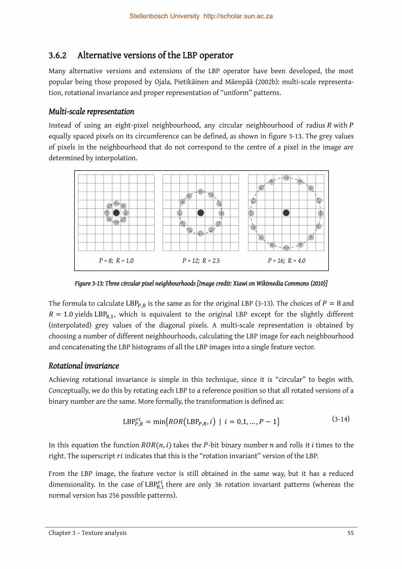
Chapter 3 – Texture analysis 55
3.6.2 Alternative versions of the LBP operator Many alternative versions and extensions of the LBP operator have been developed, the most popular being those proposed by Ojala, Pietikäinen and Mäenpää (2002b): multi-scale representa-tion, rotational invariance and proper representation of “uniform” patterns.
Multi-scale representation Instead of using an eight-pixel neighbourhood, any circular neighbourhood of radius 𝑅 with 𝑃 equally spaced pixels on its circumference can be defined, as shown in figure 3-13. The grey values of pixels in the neighbourhood that do not correspond to the centre of a pixel in the image are determined by interpolation.
The formula to calculate LBP𝑃,𝑅 is the same as for the original LBP (3-13). The choices of 𝑃 = 8 and 𝑅 = 1.0 yields LBP8,1, which is equivalent to the original LBP except for the slightly different (interpolated) grey values of the diagonal pixels. A multi-scale representation is obtained by choosing a number of different neighbourhoods, calculating the LBP image for each neighbourhood and concatenating the LBP histograms of all the LBP images into a single feature vector.
Rotational invariance Achieving rotational invariance is simple in this technique, since it is “circular” to begin with. Conceptually, we do this by rotating each LBP to a reference position so that all rotated versions of a binary number are the same. More formally, the transformation is defined as:
In this equation the function 𝑅𝑂𝑅(𝑛, 𝑖) takes the 𝑃-bit binary number 𝑛 and rolls it 𝑖 times to the right. The superscript 𝑟𝑖 indicates that this is the “rotation invariant” version of the LBP.
From the LBP image, the feature vector is still obtained in the same way, but it has a reduced dimensionality. In the case of LBP8,1𝑟𝑖 there are only 36 rotation invariant patterns (whereas the normal version has 256 possible patterns).
Figure 3-13: Three circular pixel neighbourhoods [Image credit: Xiawi on Wikimedia Commons (2010)]
LBP𝑃,𝑅𝑟𝑖 = min{𝑅𝑂𝑅(LBP𝑃,𝑅 , 𝑖) | 𝑖 = 0,1,… , 𝑃 − 1} (3-14)
P = 8; R = 1.0 P = 12; R = 2.5 P = 16; R = 4.0
Stellenbosch University http://scholar.sun.ac.za

Chapter 3 – Texture analysis 56
Representation of uniform patterns Ojala, Pietikäinen and Mäenpää (2002b) observed that certain groups of closely related LBPs represent fundamental properties of texture. In their experiments, on average 70% of images were comprised of these fundamental patterns.
To formally define “uniform” patterns, a uniformity measure 𝑈 was introduced as the number of 0/1 and 1/0 transitions in a binary pattern:
As indicated by the left-hand term of (3-16), the 1/0 and 0/1 transitions are circular, that is, if the first and last digits of a binary pattern differ, this counts as a transition.
The binary patterns 11111111 and 00000000 are the only two patterns to have 𝑈 = 0, as there are no 0/1 or 1/0 transitions. The seven patterns 11111110, 11111100, ..., 10000000 have 𝑈 = 2 as there is exactly one 0/1 transition and one 1/0 transition in each pattern. 𝑈 = 1 is not possible. Patterns are designated “uniform” when 𝑈 ≤ 2, which means that there are exactly 𝑃 + 1 uniform patterns in a circular neighbourhood of 𝑃 pixels. (In the example given here, 𝑃 = 8 and there are 2 + 7 = 9 uniform patterns).
The definition of the rotation invariant texture descriptor that includes a measure of uniformity is:
In this equation, 𝑍 is a function that returns the number of zeros in a binary pattern, for example 𝑍(11111000) = 3. The superscript 𝑟𝑖𝑢2 indicates the use of rotation invariant uniform patterns with 𝑈 ≤ 2.
The feature vector is still obtained in the same way from the LBP image (it is the histogram counts of the LBPs present in the image), but now has 𝑃 + 2 dimensions since there are only 𝑃 + 2 different LBP possibilities.
3.6.3 Applications in the process industries Although there are many potential application areas for LBP texture analysis in the process industries, there have been few successful implementations. The first two industrial LBP case studies involved the prediction of grain mixture compositions and surface quality inspection of metal strips (Pietikaeinen et al., 1994).
Combined LBP and colour features were used to detect and recognise defect types on wooden surfaces (Mäenpää et al., 2003a). In another study by Mäenpää and others (2003b), LBPs were used together with Self-Organising Map classification in a real-time paper inspection problem. In an application to quality control of ceramic tile production lines, LBP feature extraction and two
𝑈(LBP𝑃,𝑅) = |𝑠(𝑔𝑐 , 𝑔𝑃−1) − 𝑠(𝑔𝑐 , 𝑔0)| +∑|𝑠(𝑔𝑐 , 𝑔𝑝) − 𝑠(𝑔𝑐 , 𝑔𝑝−1)|
𝑃−1
𝑝=1
(3-15)
LBP𝑃,𝑅
𝑟𝑖𝑢2 = {𝑍(LBP𝑃,𝑅)
𝑃 + 1 if 𝑈(LBP𝑃,𝑅) ≤ 2 otherwise
(3-16)
Stellenbosch University http://scholar.sun.ac.za

Chapter 3 – Texture analysis 57
colour texture analysis methods were compared (López et al., 2008). All of the approaches were able to predict surface grades with very high accuracy.
A combined method consisting of LBP representation, followed by GLCM calculation, edge detection and Haralick feature extraction was used to classify different stone types (Ershad, 2011). The combined method achieved better results than either of the LBP or GLCM methods alone.
The applications of LBP features in the process industries are more numerous than applications of textons and steerable pyramids. This could be due to the straightforward LBP algorithm and low computational requirements. However, the range of applications is not very diverse, as they mostly involve surface grading. It is concluded that the LBP method is worth investigating as an image analysis algorithm for the online prediction of process quality variables, since the approach appears to be promising, but has not yet been widely applied.
3.7 Comparison between texture analysis methods In this section the five texture analysis methods discussed in sections 3.2 to 3.6 are compared in terms of important properties and characteristics. A summary of this comparison is shown in table 3-2.
Table 3-2: Comparison of properties and characteristics of five texture analysis methods
It is expected that the steerable pyramid, LBP and texton approaches could offer some advantages over the traditional methods, due to their advanced properties. Steerable pyramids offer an advantage over wavelets, since the representation is rotation and translation invariant to some extent. Although it is a transform-based approach and therefore no texture neighbourhood is used, higher-order statistical features are extracted based on global representations of the image as well as local texture neighbourhoods, as proposed by Portilla and Simoncelli (2000). It is also inherently a multiscale approach, which is thought to be advantageous since textures typically contain both local and global characteristics (Campbell & Robson, 1968).
In the texton approach ideas from statistical, structural and transform-based texture analysis methods are unified. The spatial domain filtering employed makes it a transform-based approach, but the underlying principle is that the texture consists of textural primitives (structural approach)
Method Type Texture neighbourhood
Rotation invariant? Multiscale?
GLCMs Statistical Pixel pairs To some extent No Wavelets Transform-based None No Yes Steerable pyramids
Statistical, transform-based
None, but local statistics To some extent Yes
Textons Statistical, structural, transform-based Local Yes To some extent
LBPs Statistical, structural Local Can be No
Stellenbosch University http://scholar.sun.ac.za

Chapter 3 – Texture analysis 58
that have a certain statistical probability of occurring in a given texture. The implementation in this work is also entirely rotation invariant due to the particular choice of filter set that was used. Since the various filters in the filter bank differ in size, the method also incorporates information at multiple scales to some extent.
The LBP operator combines the statistical and structural models of texture (Mäenpää & Pietikäinen, 2005). Since each model describes specific types of features, this combination can result in a more complete textural description. The original version of the LBP was not rotation invariant, but a simple extension remedies this fact (Ojala et al., 2002b). When applying the LBP operator on texture neighbourhoods with several radii, the feature vectors obtained for each neighbourhood can be concatenated to allow for a small degree of multiscale representation, although this was not implemented in this work.
A downside of both the GLCM and LBP approaches is that these methods cannot be used to analyse images at multiple resolutions. The performance of these methods would be influenced by the resolution of the original image used, which can make the results case-specific. A solution that could alleviate this problem is to optimise the resolution of the image to be analysed as a hyperparameter for these two methods.
3.8 Classification In supervised classification the data are split into training and testing sets, allowing the test data to be assigned the most probable class based on a model built using the training data. In the current work two supervised classifiers are considered: a K-nearest neighbours classifier (K-NN) and discriminant analysis (DA).
Although several advanced classifiers exist, for instance neural networks or support vector machines (SVMs), the focus of this work is on texture feature extraction and not on classification. The above-mentioned two common classifiers were therefore chosen to illustrate the discriminative capabilities of the various texture feature sets, and not necessarily to build the most optimal classification model possible.
3.8.1 K-nearest neighbours In K-nearest neighbour (K-NN) classification, given a set of training data points with known labels, a new data point is assigned the label of its closest neighbour in the feature space. The method is sensitive to irrelevant features, and it may therefore be necessary to specify 𝐾𝑁 > 1 nearest neighbours, from which the class label of a test data point is determined by majority rule. The optimal 𝐾𝑁 for a specific problem can be determined using cross-validation on the training set. Cross-validation will be described in detail in section 4.3.2 (p. 73).
A Euclidean distance metric is commonly used to determine the distance between data points. For two points 𝒑 = (𝑝1, 𝑝2, … , 𝑝𝐿) and 𝒒 = (𝑞1, 𝑞2, … , 𝑞𝐿) in a 𝑀 -dimensional feature space, the Euclidean distance between them, 𝐷𝐸(𝒑, 𝒒), is given by:
Stellenbosch University http://scholar.sun.ac.za

Chapter 3 – Texture analysis 59
The texture analysis approaches that extract histograms as features (LBPs and textons) are frequently followed by “histogram comparison” as a classification technique. This is identical to a 1-nearest neighbour classifier, but with a 𝜒2 distance metric 𝐷𝜒2:
It has been found that the specific choice of distance metric does not significantly affect classification accuracies in histogram comparison (Varma & Zisserman, 2004).
K-NN was selected as a classifier in this work for its simplicity and its ability to learn complex decision surfaces. Another advantage of K-NN is that only one hyperparameter (𝐾𝑁) has to be optimised.
3.8.2 Discriminant analysis In discriminant analysis (DA) the goal is to find a set of weights 𝒘 such that the linear combination of 𝒘 and the training data 𝒙𝑡𝑟𝑎𝑖𝑛 results in maximal separation between the classes. This “separation” is quantified in terms of the between-class scatter 𝑆𝐵 and the total within-class scatter 𝑆𝑊. If 𝜇 is the overall mean and 𝜇𝑖 is the mean of class 𝑖, the between-class scatter is given by:
for a 𝑘-class problem. For maximal separation, 𝑆𝐵 should be maximised. The within-class scatter is:
where Σ𝑖 is the covariance matrix of class 𝑖. 𝑆𝑊 should be minimised. Both these criteria can be satisfied by maximising the Rayleigh quotient ℛ(𝒘), thus determining the optimal weights 𝒘:
Each observation 𝑥 in the data set 𝒙 can be projected onto the subspace that results in maximal class separation:
𝐷𝐸(𝒑, 𝒒) = √∑(𝑞𝑖 − 𝑝𝑖)2
𝑀
𝑖=1
(3-17)
𝐷𝜒2(𝒑, 𝒒) =∑
(𝑞𝑖 − 𝑝𝑖)2
2(𝑝𝑖 + 𝑞𝑖)
𝑀
𝑖=1
(3-18)
𝑆𝐵 =
1
𝑘∑(𝜇𝑖 − 𝜇) ∙ (𝜇𝑖 − 𝜇)
𝑇
𝑘
𝑖=1
(3-19)
𝑆𝑊 =∑Σ𝑖
𝑘
𝑖=1
(3-20)
max𝒘ℛ(𝒘) =
𝒘𝑻𝑆𝐵𝒘
𝒘𝑻𝑆𝑊𝒘 (3-21)
𝑥′ = 𝑥 × 𝒘 (3-22)
Stellenbosch University http://scholar.sun.ac.za

Chapter 3 – Texture analysis 60
Here the projected version of 𝑥 is denoted by 𝑥′. Data points are then classified according to the maximum a-posteriori probability rule:
In (3-23), �� is the predicted classification and 𝑘 is the number of classes. ��(𝑗|𝑥′) is the posterior probability of class 𝑗 for observation 𝑥′, that is, the product of the prior probability that 𝑥′ belongs to class 𝑗 and the multivariate Gaussian density function. 𝐶(𝑦|𝑗) is the cost of classifying an observation of classifying an observation from class 𝑗 into class 𝑦. In this work, the cost function was set equal to 0 when 𝑗 = 𝑦 (when the observation is correctly classified), and 1 otherwise.
In DA the assumption is made that all features of data points in a class 𝑖 are normally distributed. The constraints placed on the covariance matrices of the classes determine the type of classifier obtained. In the case of linear discriminant analysis (LDA), it is assumed that the covariance matrices of all classes are equal. If, in addition, the covariance matrix estimate is diagonal, a linear naïve Bayes classifier is obtained. Without the equal covariance matrix assumption the result is a quadratic discriminant analysis (QDA) problem, and if the covariance matrix is also diagonal, it becomes a quadratic naïve Bayes classifier. Note that the naïve Bayes classifiers obtained in this way are specific versions of naïve Bayes classifiers where the variables from each class are assumed to be normally distributed (this assumption is not generally required for naïve Bayes classifiers). A summary of the covariance matrix properties for the different classifiers is shown in table 3-3.
Table 3-3: Covariance matrix properties for different discriminant analysis classifiers
3.9 Conclusions This chapter has given an overview of several texture analysis methods and their applications in the process industries. GLCMs and wavelets have been applied successfully in many process applications, but applications of the more advanced steerable pyramids, textons and LBPs are scarce. Additionally, the different texture analysis methods have seldom been compared in a structured way, and thus it is difficult to draw any conclusions with regard to their relative performance in process applications. Although based on only a few case studies that compared GLCMs and wavelets, it does seem as though wavelets have outperformed GLCMs more often than not.
A summary of the number of research papers in process engineering applications found for each method is shown in table 3-4.
�� = arg min⏟
𝑦=1,2,…,𝑘
∑ ��(𝑗|𝑥′)𝐶(𝑦|𝑗)
𝑘
𝑗=1
(3-23)
Covariance matrix property Covariance matrix of all classes equal
Covariance matrix of all classes not equal
Off-diagonal entries are not zero LDA QDA Off-diagonal entries are zero Linear naïve Bayes Quadratic naïve Bayes
Stellenbosch University http://scholar.sun.ac.za

Chapter 3 – Texture analysis 61
Table 3-4: Number of research papers in process applications for each texture analysis method
The GLCM and wavelet approaches are well established and have found their way into many process applications. The three other approaches considered (steerable pyramids, LBPs and textons) are seen as state-of-the-art in texture analysis literature, but have not extensively been applied in the process industries. Considering the attention that steerable pyramids, textons and LBPs have received in general texture analysis literature, it is concluded that it would be worthwhile to perform a quantitative investigation into the aptness of these methods for the development of vision-based inferential sensor algorithms in the process industries.
Method K-NN DA Regression / other Total GLCM 5 7 6 18 Wavelets 7 6 12 25 Steerable pyramids 0 0 1 1 Texton 1 0 1 2 LBP 1 2 3 6
Stellenbosch University http://scholar.sun.ac.za

Chapter 4 Materials and methods
In this chapter the data sets and image classification framework used in this work are discussed. The image data sets obtained from three case studies are described and the implementation details for the five texture feature extraction methods and two classification algorithms are provided.
Stellenbosch University http://scholar.sun.ac.za

Chapter 4 – Materials and methods 63
4.1 Introduction The primary objective of this study is to compare the use of advanced image texture analysis methods to baseline texture analysis methods for the prediction of key process quality variables in specific process engineering applications. Three specific process monitoring case studies were investigated:
I. the classification of platinum flotation froths into platinum grade categories, II. the classification of coal particles into fines fraction categories, and
III. the classification of hydrocyclone underflows into particle size categories.
The use of inferential sensors involves two stages: a development stage and an implementation stage. The focus of this work is on the development of algorithms for vision-based inferential sensors using texture classification, for which a general framework has been presented in chapter 2 (figure 2-3, page 18). The following details are specific to this work and were added to this general framework for vision-based inferential sensing:
the pre-processing step consists of cropping and resizing, conversion to greyscale and image normalisation,
the dimensionality reduction step consists of textural feature extraction (five methods), feature normalisation and optionally PCA, and
in the modelling step, classification (with two methods) is done.
A framework showing these details is depicted in figure 4-1, indicating also the algorithm inputs and outputs.
Five texture feature extraction algorithms were employed within this framework:
1. grey-level co-occurrence matrices (GLCMs), 2. wavelets, 3. steerable pyramids, 4. textons and 5. local binary patterns (LBPs).
The first two methods, GLCMs and wavelets, are considered as baseline methods, while the last three methods are more advanced and their uses in the process industries are not as well-established.
Stellenbosch University http://scholar.sun.ac.za
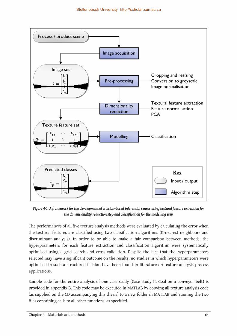
Chapter 4 – Materials and methods 64
The performances of all five texture analysis methods were evaluated by calculating the error when the textural features are classified using two classification algorithms (K-nearest neighbours and discriminant analysis). In order to be able to make a fair comparison between methods, the hyperparameters for each feature extraction and classification algorithm were systematically optimised using a grid search and cross-validation. Despite the fact that the hyperparameters selected may have a significant outcome on the results, no studies in which hyperparameters were optimised in such a structured fashion have been found in literature on texture analysis process applications.
Sample code for the entire analysis of one case study (Case study II: Coal on a conveyor belt) is provided in appendix B. This code may be executed in MATLAB by copying all texture analysis code (as supplied on the CD accompanying this thesis) to a new folder in MATLAB and running the two files containing calls to all other functions, as specified.
Figure 4-1: A framework for the development of a vision-based inferential sensor using textural feature extraction for the dimensionality reduction step and classification for the modelling step
Process / product scene
Image acquisition
Dimensionality
reduction
Modelling
Key
Input / output
Algorithm step
Image set
Pre-processing
Texture feature set
Predicted classes
Cropping and resizing
Conversion to greyscale
Image normalisation
Textural feature extraction
Feature normalisation
PCA
Classification
Stellenbosch University http://scholar.sun.ac.za

Chapter 4 – Materials and methods 65
The remainder of this chapter is organised as follows. Section 4.2 gives an overview of the three case studies used, and also serves as a discussion of the image acquisition step. Section 4.3 further elaborates on the texture classification framework by providing data partitioning, cross-validation and testing details. The remainder of the framework is discussed in sections 4.4 (pre-processing), 4.5 (dimensionality reduction) and 4.6 (modelling). The chapter ends with an explanation of the various performance evaluation methods used to analyse the results in section 4.7, and a summary in section 4.8.
4.2 Case studies The first step in any vision-based algorithm is the acquisition of image data through some sort of imaging device. The imaging device is the “eyes” of the machine vision system and could be a standard digital camera, video camera, microscope, ultrasound scanner or any other specialised apparatus.
In the supervised classification approach followed here, it is also required to collect data of the response variable – in the final data set each image should be labelled according to its class (the variable to be inferred). This section provides the details on the image acquisition and labelling procedure for each case study.
4.2.1 Case study I: Platinum flotation froths Background on froth flotation has been provided in section 2.4.1, together with a review of vision-based inferential sensing applications to froth flotation.
Case study I involves a platinum group metal (PGM) froth flotation process at the Mogalakwena North concentrator of Anglo American Platinum. The data for this case study was collected by Marais (2010) in collaboration with graduates employed by Anglo American Platinum. Full details of the experimental procedure may be found in the MSc thesis of Marais (2010); a brief summary is provided here.
A video camera was mounted above a primary cleaner flotation cell to record image data of the froth. Over a period of four hours, six step changes were made to the air flow rate of the concentrator cell, allowing the cell to stabilise between each step change. After each step, the point in time where steady state has been reached was visually determined by plant operators and noted. This resulted in a series of videos with image data for seven steady state periods. Froth samples were collected during each steady state period and analysed to determine the composition of the froth during each steady state period.
It should be noted that all other process variables were kept constant during collection of the data. Variables such as reagent dosages and impeller speeds could affect the process conditions significantly, but the effect of these variables could not be tested in this experiment. As it stands, the froth grade is correlated with the input air flow rate, and therefore it is possible that any model that is built can actually only predict air flow rate and not grade.
Stellenbosch University http://scholar.sun.ac.za

Chapter 4 – Materials and methods 66
Furthermore, another point of note is that the lighting conditions changed during the course of the experiment, despite reasonable effort being made to keep the lighting consistent (Marais, 2010). Therefore, in this particular case study the use of colour features is not recommended, as the colour may have changed simply due to varying lighting conditions.
The relative platinum grades from the assay results are shown in the middle column of table 4-1.
Table 4-1: Platinum assay results and regrouping into classes
From all steady state sections in the videos, every 30th frame (corresponding to roughly every second) was extracted. For computational reasons it was not feasible to extract all frames, and no significant loss of data is expected when the data is subsampled in this manner, since consecutive frames are very similar. The images obtained were regrouped into four classes as shown in the last column of table 4-1. The 6th sample was omitted because its relative Pt grade (0.28) is close to the relative grades of class 4 (0.11 to 0.16) and class 3 (0.38 to 0.40). The goal here was to test classification on discrete classes, and it is suggested that the 6th sample may be too similar to class 3 or 4 to be discerned. When performing regression, the inclusion of this data is more appropriate.
The resulting image data set consisted of 2720 images in four platinum grade classes, as summarised in table 4-2. An example image from each class is shown in figure 4-2. The goal of the image classification algorithm was to predict these platinum grade classes from froth images.
Table 4-2: Platinum grade classes
Sample Relative Pt grade Class 1 1.00 1 2 0.59 2 3 0.38 3 4 0.11 4 5 0.16 4 6 0.28 None 7 0.40 3
Class Relative Pt grade Number of images 1: Very high Pt grade 1.00 780 2: High Pt grade 0.59 480 3: Medium Pt grade 0.38 – 0.40 678 4: Low Pt grade 0.11 – 0.16 782
Stellenbosch University http://scholar.sun.ac.za

Chapter 4 – Materials and methods 67
Class 1 Class 2
Class 3 Class 4
Figure 4-2: Example platinum froth flotation images
4.2.2 Case study II: Coal on a conveyor belt Background on processes where the conveyance of particulate matter is concerned has been provided in section 2.4.2, together with a review on appropriate inferential sensing studies.
This second case study entails the estimation of the percentage fine particles in coal on a conveyor belt. In a laboratory experiment performed by Aldrich and others (2010), coal was sieved and separated into coarse (> 6 mm) and fine (< 6 mm) fractions. These fractions were mixed in varying quantities to prepare seven different blends containing 0%, 20%, 40%, 50%, 60%, 80% and 100% fines by mass. Ten samples of each blend were created. To simulate industrial conditions, the samples were placed on a pilot plant conveyor belt. Images of the samples were captured with a digital camera.
It should be noted that this experimental setup was not very similar to what is found in an industrial plant. In an industrial process where coal is fed to gasifiers, the coal undergoes a wet screening process, is subject to layering (the coarse particles tend to be loaded on top of the fine particles) and the upper limit for the desired fines percentage is only 10% (Mans, 2013, personal communication, 11 July). On the contrary, in the laboratory experiment dry coal was used and the layering of coal particles was not simulated. Images of coal where the fines fractions were close to
Stellenbosch University http://scholar.sun.ac.za

Chapter 4 – Materials and methods 68
the 10% upper limit would have been useful, but were not collected. As it is, this case study serves as a proof of concept only.
Images of the seven blends were re-grouped into three categories “coarse”, “intermediate” and “fine”, and each of the 70 images were subdivided into four non-overlapping patches in to increase the size of the data set to 280 images. A summary of this data set is shown in table 4-3, and figure 4-3 shows example images from each class. For this data set, the goal of the image classification algorithm was to predict the fines fraction classes from coal images.
Table 4-3: Fines fraction in coal classes
Class Fines (%) Number of images 1: Coarse 0 – 20 80 2: Intermediate 40 – 60 120 3: Fine 80 – 100 80
Class 1: Coarse
Class 2: Intermediate
Class 3: Fine
Figure 4-3: Example coal particle images. The white circle present in each image is a South African five-rand coin with a diameter of 26 mm, which gives an indication of scale.
0% fines
20% fines
40% fines
50% fines
60% fines
80% fines
100% fines
Stellenbosch University http://scholar.sun.ac.za

Stellenbosch University http://scholar.sun.ac.za

Chapter 4 – Materials and methods 70
Class 1: Coarse Class 2: Intermediate Class 3: Fine
Figure 4-5: Example images from the hydrocyclone underflow data set
4.3 Data partitioning, cross-validation and testing In a typical machine learning setup, data is partitioned into training and test data. Training data is used to determine the model parameters (for example the coefficients in a PCA model), and then test data is used as input to the trained model to predict how well the algorithm will perform in a real application. For all experiments in this study, approximately 75% of the images in each class were used for training, with the remaining 25% being reserved for testing.
When there are various hyperparameter settings for an algorithm (such as the type of wavelet used, or the number of nearest neighbours 𝐾𝑁 in the K-NN algorithm), validation may be used to determine the optimal hyperparameter set. This is done by keeping a portion of the training data aside as validation data, and testing with these data. The best hyperparameter setting is that which results in the lowest validation error.
To reduce the effect that variability in the data may have on the validation error, a method called cross-validation may be used. In this work, five-fold cross-validation was used, which requires the training data to be split into five approximately equally sized folds. The data partitioning procedures for each of the case studies are detailed in section 4.3.1. More information regarding cross-validation and testing are given in sections 4.3.2 and 4.3.3, respectively.
4.3.1 Data partitioning
Case study I: Platinum flotation froth One of the most popular data partitioning methods is random subdivision into training, validation and test sets. However, although random partitioning has been used in previous work on the same data set (Marais, 2010; Marais & Aldrich, 2011), a different approach was followed in this work. This is motivated by the fact that the image data for this case study are a series of frames extracted from videos of flotation froths. As such, it is possible that sequential images can be correlated to one another, even when only every 30th frame is used (as in this case study).
Stellenbosch University http://scholar.sun.ac.za

Chapter 4 – Materials and methods 71
Examples of two images that occur 30 frames apart in the original video footage are shown in figure 4-6, and illustrate that there is indeed a high degree of similarity between sequential images in the data set. If such a data set is randomly partitioned, the training and test sets will be very similar, and the test error would not be a true estimation of out-of-sample performance. Therefore, instead of random partitioning, contiguous blocks of images were used as training and test data, and 40 images in between each pair of blocks (covering 20 seconds in the video) were removed from the data set to simulate an independent test set. Similarly, the training data were subdivided into five contiguous folds. A disadvantage of partitioning the data in this way is that the training data may not be truly representative, but this approach is necessary to guard against overfitting (overfitting is when the model learns to fit the peculiarities present in the training set, causing poor generalisation to any new data that is not part of the training set).
The partitioning of the 2720 images in the data set is illustrated in figure 4-7, with the number of images per class in each set resulting from this partitioning in table 4-5.
Table 4-5: Sizes of training and test sets in froth flotation data set
Figure 4-6: Two images in the flotation froth data set occurring 30 frames apart in the original video footage.
Class Number of images
Training Test Total 1 575 (115 per fold) 185 760 2 350 (70 per fold) 110 460 3 489 (98 per fold) 149 638 4 567 (113 per fold) 175 742
Totals: 1981 619 2600
Stellenbosch University http://scholar.sun.ac.za

Chapter 4 – Materials and methods 72
Case study II: Coal on a conveyor belt The 280 images in the coal data set were randomly partitioned such that 75% of the images in each class were used for training, with the remaining 25% being reserved for testing. Here the contiguous block approach was not necessary, as there is not any correlation in time between sequential images.
The training images were further randomly subdivided into five approximately equally sized folds for cross-validation. The number of images per class in each set is shown in table 4-6.
Figure 4-7: Partitioning of froth flotation data set
Class 11.00 rel. Pt
780 images
Class 20.59 rel. Pt
480 images
Class 3a0.38 rel. Pt
300 images
Class 4a0.11 rel. Pt
362 images
Class 4b0.16 rel. Pt
420 images
Class 3b0.40 rel. Pt
378 images
Training
Test
Training
Test
Training
Test
Training
Test
Training
Test
Training
Test
Image 1
Image 2
⋮
Image 2720
Image seq
uen
ce
Fold 1
Fold 2
Fold 5
⋮
Fold 1Fold 2
Fold 5
⋮
⋮
⋮
⋮
Fold 1Fold 2
Fold 5⋮
REMOVE
REMOVE
REMOVE
REMOVE
REMOVE
REMOVE
Stellenbosch University http://scholar.sun.ac.za

Chapter 4 – Materials and methods 73
Table 4-6: Sizes of training and test sets in coal data set
Case study III: Hydrocyclone underflows The 300 images in this case study were randomly partitioned into training and test sets and cross-validation folds. The method of partitioning was exactly the same as for case study II, and again the contiguous block approach was not necessary. The number of images per class in each set is shown in table 4-7.
Table 4-7: Sizes of training and test sets in hydrocyclone data set
4.3.2 Cross-validation In 𝑍-fold cross-validation, the training data is split into 𝑍 approximately equally sized subsamples or “folds”, and the validation process is repeated 𝑍 times. During repetition 𝑧 (𝑧 = 1,2, … , 𝑍), the images in fold 𝑧 are used as validation data, with the images in the remaining 𝑍 − 1 folds being used as training data. The hyperparameter set with the lowest validation error, averaged across all folds, is selected as the best hyperparameter set for the algorithm and used during the final training and testing phase. The same data partitioning into folds were used for all hyperparameter sets tested.
Pseudocode for the cross-validation procedure used in this work is given in figure 4-8. This information is also depicted visually in figures 4-9 and 4-10.
Class Number of images
Training Test Total 1 60 (12 per fold) 20 80 2 90 (18 per fold) 30 120 3 60 (12 per fold) 20 80
Totals: 210 70 280
Class Number of images
Training Test Total 1 30 (6 per fold) 10 40 2 116 (23 per fold) 38 154 3 80 (16 per fold) 26 106
Totals: 226 74 300
Stellenbosch University http://scholar.sun.ac.za

Chapter 4 – Materials and methods 74
given number of folds Z; given all training images, partitioned into folds 1, 2, ..., Z; given feature extraction hyperparameter options H_F; given classification hyperparameters options H_C; given known class information (labels) of all training images;
% do cross-validation for each cross-validation run z = 1, 2, ..., Z
training images = all training images not in fold z; validation images = all training images in fold z;
for each feature extraction hyperparameter combination i in H_F for each classification hyperparameter combination j in H_C training features = features extracted from ...
training images using hyperparameter combination i; classifier = model trained using training features ...
and hyperparameter combination j; validation features = features extracted from validation ...
images using hyperparameter combination i; predicted labels = classes of validation images ...
predicted by classifier; error(z,i,j) = fraction incorrectly predicted labels ...
of validation images; end end
end
% calculate average errors to determine optimal hyperparameter set for each i for each j error(i,j) = average of error(z,i,j) across all z; end end
best hyperparameter combination = i and j with lowest error(i,j);
Figure 4-8: Pseudocode for 𝒁-fold cross-validation on hyperparameter combinations (𝒊, 𝒋)
Stellenbosch University http://scholar.sun.ac.za

Chapter 4 – Materials and methods 75
Figure 4-9: Detailed development of an inferential sensor showing the calculation of error rates 𝓔 ,𝒊,𝒋 for 𝒁-fold cross-validation.
Error rate ____
Classification
hyperparameters ___
Feature extraction
hyperparameters ___
Rep
eat
for
each
fo
ld
Rep
eat
for
each
hyp
erp
ara
met
er c
om
bin
ati
on
Process / product scene
Image acquisition
Image set
Data partitioning
Training images Test images
Model training
Predicted class
information
Trained classifier
Training images for CV Validation images
Dimensionality
reduction
Dimensionality
reduction
Model application
Known class
information
Dimensionality
reduction parameters
Key
External input
Step input / output
Final output
Algorithm step
Training texture
feature set
Validation texture
feature set
Pre-processing
Stellenbosch University http://scholar.sun.ac.za

Chapter 4 – Materials and methods 76
Figure 4-9 adds more detail to the diagram explaining the development of a visual-based inferential sensor, as shown in the beginning of this chapter (figure 4-1, p. 64). It includes the data partitioning step (as explained in section 4.3.1) and the procedure for calculating error rates ℰ𝑧,𝑖,𝑗 for cross-validation. The subscript 𝑧 refers to the fold, 𝑖 indicates that the 𝑖th feature extraction hyperparame-ter set was used and 𝑗 indicates that the 𝑗th classification hyperparameter set was used.
An error rate for a specific combination of 𝑧, 𝑖 and 𝑗 is simply the fraction of incorrectly predicted labels of the validation data, and is calculated by comparing the predicted labels (class information) of the images with the known labels:
If there are 𝑁𝑣𝑎𝑙 validation images, 𝒞𝑝 and 𝒞𝑘 are vectors of length 𝑁𝑣𝑎𝑙 containing the predicted and known class labels, respectively. The “==” is a logical equal operator, so that 𝐴 == 𝐵 returns 1
Figure 4-10: The error rates 𝓔 ,𝒊,𝒋 are used to determine the optimal hyperparameter combination {𝓗
,𝓗 }. Here 𝒉𝒇 is the number of feature extraction hyperparameters settings and 𝒉𝒄
is the number of classification hyperparameters
ℰ𝑧,𝑖,𝑗 = 1 −
∑ (𝒞𝑝,𝑛 == 𝒞𝑘,𝑛)𝑁 𝑛=1
𝑁𝑣𝑎𝑙 (4-1)
Average
Average
Average
Minimum
⋮
⋮
⋮
⋮
⋮
⋮
⋮
⋮
Stellenbosch University http://scholar.sun.ac.za

Chapter 4 – Materials and methods 77
when 𝐴 = 𝐵 and 0 when 𝐴 ≠ 𝐵. The operator is applied in a pairwise fashion to each entry 𝒞𝑝,𝑛 and 𝒞𝑘,𝑛 of 𝒞𝑝 and 𝒞𝑘.
The details regarding the dimensionality reduction and modelling steps in this diagram will be explained in sections 4.5 and 4.6, respectively.
Figure 4-10 shows how the error rates ℰ𝑧,𝑖,𝑗 are used to determine the optimal hyperparameter combination. Let the set of possible feature extraction hyperparameters be 𝓗 = {ℋ𝐹,1,ℋ𝐹,2, … ,ℋ𝐹,ℎ𝑓} and let the set of possible classification hyperparameters be 𝓗 =
{ℋ𝐶,1,ℋ𝐶,2, … ,ℋ𝐶,ℎ𝑐}, where ℎ𝑓 is the number of feature extraction hyperparameter settings and ℎ𝑐 is the number of classification hyperparameter settings. The error rate ℰ𝑖,𝑗 for each hyperparameter combination {ℋ𝐹,𝑖 , ℋ𝐶,𝑗} is calculated as the average error rate across all folds 𝑧 = 1,2, … , 𝑍 for that hyperparameter combination:
The minimum ℰ𝑖,𝑗 is then determined, and the hyperparameter combination that led to this minimum error rate is the optimal combination {ℋ𝐹 ,ℋ𝐶
}. These optimal hyperparameters will be used during the final training and test phase.
4.3.3 Testing Once the optimal hyperparameters have been determined, the final training and testing is performed, as shown in figure 4-11. The model is retrained using all training data, and tested to determine the predicted class labels for the test data (𝒞𝑝), and hence the final error rate:
Here 𝑁𝑡𝑒𝑠𝑡 is the number of test images, and 𝒞𝑝 and 𝒞𝑘 are vectors of length 𝑁𝑡𝑒𝑠𝑡 containing the predicted and known class labels for the test images, respectively.
ℰ𝑖,𝑗 =
∑ ℰ𝑧,𝑖,𝑗𝑍𝑧=1
𝑍 (4-2)
ℰ𝑡𝑒𝑠𝑡 = 1 −
∑ (𝒞𝑝,𝑛 == 𝒞𝑘,𝑛)𝑁 𝑛=1
𝑁𝑡𝑒𝑠𝑡 (4-3)
Stellenbosch University http://scholar.sun.ac.za

Chapter 4 – Materials and methods 78
Figure 4-11: Detailed framework for the development of an inferential sensor, showing training and testing procedures.
Error rate ____
Classification
hyperparameters ___
Feature extraction
hyperparameters ___
Process / product scene
Image acquisition
Image set
Data partitioning
Training images Test images
Model training
Predicted class
information
Trained classifier
Dimensionality
reduction
Dimensionality
reduction
Model application
Known class
information
Dimensionality
reduction parameters
Key
External input
Step input / output
Final output
Algorithm step
Training texture
feature set
Test texture
feature set
Pre-processing
Stellenbosch University http://scholar.sun.ac.za
Chapter 4 – Materials and methods 79
4.4 Pre-processing Pre-processing involves all alterations that have to be made to get the original image data in the correct format for feature extraction. In this work, pre-processing consisted of cropping, resizing, conversion to greyscale and normalisation.
4.4.1 Cropping and resizing In some cases images can be cropped to remove irrelevant information, such as the background.
High-resolution images place a high demand on computer memory, and therefore it may be necessary to resize images to reduce the resolution. The final resolution of the images should be the maximum possible given the hardware limitations, since low quality images can affect the results adversely. In this work images were resized using bicubic interpolation with antialiasing (Keys, 1981). With bicubic interpolation an output pixel value becomes a weighted average of the pixel values in its nearest 4-by-4 neighbourhood, while antialiasing smoothes edges to improve visual appearance.
Another reason for changing the image size is due to a limitation of the steerable pyramid implementation used in this work (Portilla & Simoncelli, 2000). The algorithm was implemented in such a way that images are required to have a width and height that is divisible by 2𝐽, where 𝐽 is the number of levels in the decomposition. To achieve this, images can be resized horizontally or vertically, or if the original aspect ratio would be drastically affected by resizing, a small portion of the image may be cropped off. It is interesting to note that the execution times of several other texture analysis algorithms are increased when the image dimensions are odd.
The cropping and resizing procedures for each case study are described in the remainder of this section.
Case study I: Platinum flotation froths Images in the flotation data set were not cropped, but they were resized to reduce the resolution from 1280 × 720 pixels to 1024 × 576 pixels.
Case study II: Coal particles on a conveyor belt Other studies that used this data set (Aldrich et al., 2010; Jemwa & Aldrich, 2012) cropped images to a central patch to minimise the effect of uneven lighting, and to remove the conveyor belt background and South African R5 coin that was used as a scale indicator. However, in this work images were not cropped, because:
a good inferential sensor should be robust to uneven lighting conditions and random artefacts (such as the R5 coin), making it desirable to retain these conditions,
the coal particle size distribution is not always uniform across an image, which means that cropping off large sections of the image skews the information available to the classification algorithm, potentially leading to worse results, and
Stellenbosch University http://scholar.sun.ac.za

Chapter 4 – Materials and methods 80
such cropping would require manual intervention, which would limit automated inferential sensing applications.
The original coal images had a resolution of 2272 × 1704 pixels, but since these were subdivided into four non-overlapping patches, each subdivision had a resolution of 1136 × 852 pixels. These were resized to 1024 × 768 pixels.
Case study III: Hydrocyclone underflows Images in the original hydrocyclone data set as obtained from Uahengo (2013) did not have identical resolutions. The first step in resizing these images was to crop each image to the minimum width (3000 pixels) and minimum height (2262 pixels) in the data set, retaining the central part of each image.
The resultant images from the first cropping step still contained a large portion of black background, and could therefore be further cropped to remove this background to some extent. The size and position of a common cropping rectangle across all images were visually determined by overlaying all images on top of each other. Appropriate coordinates for the upper-left corner of the cropping rectangle (𝑥0, 𝑦0) were determined to be (0, 100), and the size of the cropping rectangle was 2560 (width) × 2048 (height) pixels.
The final cropped images were resized from 2560 × 2048 pixels to 1280 × 1024 pixels.
4.4.2 Conversion to greyscale Traditional texture analysis methods were developed for the analysis of greyscale images, but many methods of incorporating colour or spectral information exist, such as multi-resolution multivariate image analysis (MR-MIA). Although the choice of using only greyscale information is not to be made lightly, in this work it can be motivated by the fact that colour is not expected to play an important role in any of the three case studies considered.
Image data for all three case studies were initially in RGB format. The standard formula for converting an RGB image to greyscale (4-4) was used: the greyscale image 𝐼𝐺 is an average of the 𝑹,𝑮,𝑩 components, weighted according to human perception of colours:
4.4.3 Image normalisation A common problem in vision-based sensing is inconsistent lighting conditions. If illumination varies across images, the feature extraction algorithm may incorrectly recognise this variation as a key feature. However, a good texture analysis algorithm should be robust to non-optimal lighting conditions, as this would typically be encountered in a real plant environment. Therefore, only the most basic method of correcting for lighting inconsistencies, namely normalisation, was used.
𝐼𝐺 = 0.2989𝑹+ 0.5870𝑮 + 0.1140𝑩 (4-4)
Stellenbosch University http://scholar.sun.ac.za

Chapter 4 – Materials and methods 81
To obtain a normalised image 𝐼𝑛𝑜𝑟𝑚 with zero mean and unit standard deviation from the original greyscale image 𝐼𝐺, its mean 𝜇𝐺 is subtracted and the result is divided by its standard deviation 𝜎𝐺:
Here 𝐽𝑤,ℎ is a matrix of ones with dimensions ℎ and 𝑤, the height and width of the image (required for matrix subtraction).
4.5 Dimensionality reduction In this work, the dimensionality reduction step consisted of texture feature extraction, feature normalisation and optionally PCA. The dimensionality reduction section from figure 4-11 (the detailed training and testing inferential sensor framework) is shown here as figure 4-12, which also includes the sub-steps within dimensionality reduction.
𝐼𝑁 =
𝐼𝐺 − 𝜇𝐺 ⋅ 𝐽ℎ,𝑤𝜎𝐺
(4-5)
Figure 4-12: Dimensionality reduction allows for the images to be represented by a reduced, textural feature set instead of pixels.
Feature extraction
hyperparameters ___
Training images Test images
Texture feature
extraction
Texture feature
extraction
Feature scaling
parameters
Training texture
feature set
Test texture
feature set
Key
External input
Step input / output
Algorithm step
Feature
normalisation
Feature
normalisation
PCA PCA
Dim
en
sio
nal
ity
red
uct
ion
Dim
en
sion
ality red
uctio
n
Cluster centres
PCA parameters
Texton only
Stellenbosch University http://scholar.sun.ac.za

Chapter 4 – Materials and methods 82
The main step in dimensionality reduction is texture feature extraction. The implementation details of the five different feature extraction methods that were tested in this work are given in sections 0 to 4.5.5. Section 4.5.6 details the feature normalisation method, while section 4.5.7 explains PCA.
4.5.1 Grey-level co-occurrence matrices
Description Introduced by Haralick and others (1973), the use of grey-level co-occurrence matrices (GLCMs) for textural feature extraction has become one of the most popular texture analysis methods in literature. A GLCM of an image is a concise summary of the frequencies at which grey levels occur at a specified displacement from each other. It is thus a representation of the local textural properties of an image, and several statistical features are commonly extracted from one or more GLCM to describe these textural properties. More details on GLCMs are given in section 3.2 (page 31).
Hyperparameters considered The hyperparameters that may be varied in the calculation of GLCMs, with their values considered in this work, are given in table 4-8. The number of grey levels, 𝐺, is usually not optimised in GLCM applications. However, some sources suggest that this hyperparameter is important (Clausi, 2002), and its optimisation was therefore included to allow for this possibility. The choices for the other three hyperparameters were made in accordance with popularity in literature (Haralick, 1979).
Table 4-8: GLCM hyperparameters and their considered values
Since there were five options for 𝐺 and five options for 𝐷, a total of ℎ𝑓 = 25 feature extraction hyperparameter settings were tested. For each hyperparameter setting, the following steps were carried out:
1. Given that the number of orientations was chosen as four, GLCMs were calculated at four equally spaced angles (0°, 45°, 90° and 135°).
2. A popular subset of the original Haralick statistical features was extracted from each of the four GLCMs: contrast, correlation, energy and homogeneity.
3. For each statistical feature, its average and standard deviation across all four orientations was calculated (as in Haralick, 1979).
This procedure results in a GLCM feature vector of length 4 × 2 = 8; this implementation the order of the features is {𝐶𝑂𝑁𝐴𝑉𝐺 , 𝐶𝑂𝑁𝑆𝑇𝐷 , 𝐶𝑂𝑅𝐴𝑉𝐺 , 𝐶𝑂𝑅𝑆𝑇𝐷 , 𝐸𝑁𝐸𝐴𝑉𝐺 , 𝐸𝑁𝐸𝑆𝑇𝐷 , 𝐻𝑂𝑀𝐴𝑉𝐺 , 𝐻𝑂𝑀𝑆𝑇𝐷}.
Hyperparameter Values considered Number of grey levels (𝐺) 𝐺 = 2𝑔, 3 ≤ 𝑔 ≤ 7, 𝑔 ∈ ℕ Size of displacement between grey level pairs (𝐷) 1 ≤ 𝐷 ≤ 5, 𝐷 ∈ ℕ GLCM type Symmetric (not varied) Number of orientations 4 (not varied)
Stellenbosch University http://scholar.sun.ac.za

Chapter 4 – Materials and methods 83
4.5.2 Wavelets
Description Wavelets are mathematical functions that may be used for multi-resolution analysis of images (Mallat, 1989), offering several advantages over the well-known Fourier analysis. Wavelet texture analysis usually involves the decomposition of images into horizontal, vertical and diagonal coefficient sets at multiple scales or levels. A feature set commonly extracted from this representation consists of the energies of all the coefficient sets. Wavelets are described in more detail in section 3.3 (page 35).
Hyperparameters considered In this work, three popular orthogonal wavelets were considered (table 4-9): the Haar wavelet (the same as the Daubechies wavelet with a 1-tap filter; abbreviated as ‘haar’), the Daubechies 3-tap wavelet (‘db3’) and the Symlet 4-tap wavelet (‘sym4’). Although some sources suggest that the type of wavelet used does not seem to have a large influence on the results (Chang & Kuo, 1993), these three popular wavelets were compared to allow for the possibility that the choice does affect the results significantly.
Table 4-9: Wavelet hyperparameters and their considered values
For each case study, wavelet decomposition was performed to the maximum level. The criteria for choosing the maximum level followed that of Ruttimann and others (1998) and depend on the type of wavelet and the resolution of the original image. For case studies I (flotation) and II (coal particles), the maximum level was 6, while images for case study III (hydrocyclones) could be decomposed up to the 7th level.
The energies of all sets of vertical, horizontal and diagonal coefficients were calculated, resulting in feature vectors of length 3 × 6 = 18 for the 6-level wavelet decompositions and feature vectors of length 3 × 7 = 21 for the 7-level decompositions. For a 𝐽-level decomposition, the order of the features is given by {𝐸𝐻1, 𝐸𝐻2, … , 𝐸𝐻𝐽 , 𝐸𝑉1, 𝐸𝑉2, … , 𝐸𝑉𝐽, 𝐸𝐷1, 𝐸𝐷2, … , 𝐸𝐷𝐽} where 𝐸 denotes “energy” and the subscripts 𝐻 , 𝑉 and 𝐷 denote the horizontal, vertical and diagonal components, respectively.
4.5.3 Steerable pyramids
Description The steerable pyramid is a translation- and rotation-invariant transform in multi-resolution image analysis, developed by Simoncelli and others (1992). This state-of-the-art image analysis method
Hyperparameter Values considered Wavelet type ‘haar’, ‘db3’, ‘sym4’ Decomposition level (𝐽) Maximum (not varied)
Stellenbosch University http://scholar.sun.ac.za

Chapter 4 – Materials and methods 84
has achieved considerable success in many, diverse applications, but has not yet been extensively applied in the process industries.
Portilla and Simoncelli (2000) proposed a set of visually meaningful statistical measurements, consisting of four groups, which may be extracted from the steerable pyramid representation to provide a complete textural description of an image: marginal statistics, coefficient correlations, magnitude correlations and cross-scale phase statistics. In this work, these four sets of statistics were calculated and used as features, with one exception: the means and standard deviations of the pixels in the original images, part of the “marginal statistics”, were not calculated. This is because images were normalised to have zero mean and unit variance.
Hyperparameters considered In this work a 3rd order directional derivative filter set was used to decompose images to the maximal level. For case study I (flotation), the maximum level was 5, while the images from case studies II (coal particles) and III (hydrocyclones) could be decomposed to the 6th level. Two further hyperparameters influence the statistical feature set obtained: the number of orientations included (𝑆𝑖𝑛𝑐) and the width of the square pixel neighbourhood used in the computation of local statistics (𝑊). The values considered for all of these hyperparameters are given in table 4-10.
Table 4-10: Steerable pyramid hyperparameters and their considered values
Since there were two options for 𝑆𝑖𝑛𝑐 and two options for 𝑊, a total of four hyperparameter combinations were tested. The length of a steerable pyramid feature vector is a function of 𝐽, 𝑆𝑖𝑛𝑐 and 𝑊, and ranged between 889 (𝐽 = 5, 𝑆𝑖𝑛𝑐 = 4, 𝑊 = 7) and 3272 (𝐽 = 6, 𝑆𝑖𝑛𝑐 = 6, 𝑊 = 11).
4.5.4 Textons
Description Conceptually, textons are local texture descriptors or textural “primitives”, such as blobs, edges, line terminators and line crossings (Julesz, 1981). Modern texton approaches involve image filtering and pixel clustering, with textons being defined as cluster centres in the filter response space. The features for each image are then a histogram of the textons occurring in the image (Varma & Zisserman, 2005).
The texton algorithm differs from all four other feature extraction methods in two ways:
1. The K-means clustering during training requires all images in the training images to be stored in memory at the same time, while all other methods can extract features from one image at a time. This makes the algorithm more memory intensive.
Hyperparameter Values considered Filter bank 3rd order directional derivatives (not varied) Decomposition level (𝐽) Maximum (not varied) Number of orientations (𝑆𝑖𝑛𝑐) 4, 6 Width of pixel neighbourhood (𝑊) 7, 11
Stellenbosch University http://scholar.sun.ac.za

Chapter 4 – Materials and methods 85
2. Information from the feature extraction step for training images is used in the feature extraction of test images: there is no clustering in the feature extraction of test images, but rather pixels are assigned to the cluster centres or textons that were determined during training.
Computation time The computer running time required to run the texton algorithm is worth mentioning here. The texton algorithm is extremely slow when compared to the other datasets, taking about 18 hours in average to calculate the features for one hyperparameter combination.
There are two reasons for this long computer running time. Firstly, the K-means clustering algorithm is very time-consuming, even when fully vectorised, due to the extremely large number of data points in the cluster space (each pixel in each training image becomes a 13-dimensional data point in the cluster space). Secondly, since the pixels of the training images are aggregated before clustering, the clustering step has to be repeated every time the training set changes. This means that new cluster centres 𝒯 are computed for each fold during the five-fold cross-validation, as well as for final testing (when the entire training set is used for training), which roughly multiplies the computation time that is required by six. In contrast, during the five-fold cross-validation and testing of the other feature sets, the features only have to be extracted once, and only the feature scaling and PCA (both of which are fast procedures) are repeated six times. This is also shown in figure 4-12 (p. 81), where for textons only, the parameter 𝒯 from the feature extraction step is used during the test phase.
Hyperparameters considered Several filter banks have successfully been used together with the texton approach. In this work a filter bank consisting of thirteen rotationally invariant Gabor-like filters (Schmid, 2001) was used, since this filter bank is simple to compute, has low dimensionality and yielded the best texture classification results in a previous study on the coal data set (Jemwa & Aldrich, 2012).
In the original work by Schmid (2001) and in a few subsequent studies (Varma & Zisserman, 2005; Jemwa & Aldrich, 2012), the spatial support of the largest filter in the filter bank was fixed at 49 × 49 pixels. However, other authors have found that the size of the filter support is an important factor in the overall success of the algorithm. Since many filtering approaches in literature use a smaller rather than larger support, a smaller support size of 25 × 25 pixels was also tested.
Clustering in the texton algorithm was done with the K-means algorithm. Although simple to implement, one drawback of this method is the need to pre-emptively specify the number of cluster centres or textons, 𝐾𝑇. Following Jemwa and Aldrich (2012), four values of 𝐾𝑇 were tested: 10, 20, 40 and 80.
Due to the large size of the flotation data set (case study I), only every 4th image in the training set (in chronological order) was used in the clustering step. This was necessary due to computer memory limitations, and was deemed acceptable since consecutive images are still very similar even though the original data set has already been sampled.
Stellenbosch University http://scholar.sun.ac.za

Chapter 4 – Materials and methods 86
The hyperparameters that may be varied in the texton algorithm, as well as their values considered, are summarised in table 4-11. The two options for the filter support width and four options for 𝐾𝑇 results in a total of eight hyperparameter combinations being tested.
Table 4-11: Texton hyperparameters and their considered values
The length of a texton feature vector is usually equal to the number of cluster centres chosen, 𝐾𝑇. However, during the K-means clustering step it is possible that some clusters become empty and are removed. Therefore, the number of textons is sometimes less than the specified amount of cluster centres.
4.5.5 Local binary patterns
Description The local binary pattern (LBP) is a texture analysis operator for local texture characterisation, initially proposed by Olaja and others (1994). The operator is applied to greyscale images in a pixel-wise fashion by comparing each pixel to its local pixel neighbourhood. The final textural feature set of an image is a histogram of the LBPs in the image. The underlying principles of LBP texture analysis is the same as that of the texton algorithm, but with the advantage of reduced computational complexity.
Hyperparameters considered The hyperparameters that may be varied in LBP texture analysis are the texture neighbourhood radius and sampling points pair (𝑅, 𝑃), and the mapping type, as shown in table 4-12.
Table 4-12: LBP hyperparameters and their considered values
For the hyperparameters (𝑅, 𝑃), the values (1, 8), (2.5, 12) and (4, 16) were considered, following Ojala and others (2002b). It is not feasible to increase number of sampling points to much higher than sixteen, due to the high dimensionality of the feature set that would be produced. The mapping types considered were ‘none’, rotational invariance mapping (‘ri’), uniform pattern mapping (‘u2’) and both rotational invariance and uniform pattern mapping (‘riu2’).
Hyperparameter Values considered Filter bank Schmid (not varied) Support width of largest filter (𝐹𝑆) 25, 49 Number of cluster centres (𝐾𝑇) 20, 40, 80
Hyperparameter Values considered Texture neighbourhood radius and sampling points pair (𝑅, 𝑃) (1, 8), (2.5, 12), (4, 16) Mapping type ‘none’, ‘ri’, ‘u2’, ‘riu2’
Stellenbosch University http://scholar.sun.ac.za

Chapter 4 – Materials and methods 87
The three (𝑅, 𝑃) options and four mapping type options led to twelve hyperparameter combinations being tested. The length of a LBP feature vector is initially 2𝑃, but can be reduced considerably depending on the mapping type used.
4.5.6 Feature set normalisation Once the textural feature set has been obtained by using one of the texture feature extraction methods, it is common practice to normalise the features before proceeding with further dimensionality reduction or classification. One important reason for this is due to the fact that the ranges of the various features can vary considerably. Normalisation ensures that features with large values do not overpower features with small values during the classification step.
In this work the features for the training samples were normalised to have zero mean and unit standard deviation. The normalisation for each feature 𝓕𝑡𝑟𝑛(𝑖) (column in the feature matrix 𝓕𝑡𝑟𝑛) is given by:
where 𝜇𝑡𝑟𝑛 and 𝜎𝑡𝑟𝑛 are vectors of the feature means and standard deviations, respectively. 𝑱𝑁 is a vector of ones with length 𝑁𝑡𝑟𝑛, the number of training images.
The means and standard deviations of the training features were used to standardise the test features, according to:
4.5.7 Principal component analysis Principal component analysis (PCA) finds the orthogonal axes of maximal variation in a feature set and transforms the features onto these axes. The use of PCA results in dimensionality reduction when the first 𝐶𝑣𝑎𝑟 transformed features or principal component scores are used, where 𝐶𝑣𝑎𝑟 is the number of principal component scores that explain 𝑣𝑎𝑟 percent of the variance. Thus, PCA may be used to reduce the dimensionality of extracted texture feature sets that could possibly contain redundant features. As part of the hyperparameter optimisation process, the options considered for PCA were ‘none’ (no PCA), 𝑣𝑎𝑟 = 99% and 𝑣𝑎𝑟 = 95%.
��𝑡𝑟𝑛(𝑖) =
𝓕𝑡𝑟𝑛(𝑖) − 𝜇𝑡𝑟𝑛(𝑖) ⋅ 𝑱𝑁 𝜎𝑡𝑟𝑛(𝑖)
(4-6)
��𝑡𝑒𝑠𝑡(𝑖) =
𝓕𝑡𝑒𝑠𝑡(𝑖) − 𝜇𝑡𝑟𝑛(𝑖) ⋅ 𝑱𝑁 𝜎𝑡𝑟𝑛(𝑖)
(4-7)
Stellenbosch University http://scholar.sun.ac.za

Chapter 4 – Materials and methods 88
4.6 Modelling
4.6.1 K-nearest neighbours In K-nearest neighbour (K-NN) classification, given a set of training data points with known labels, a new (test) data point is assigned the majority rule label of its 𝐾𝑁 closest neighbours in the feature space. In this work the numbers of nearest neighbours considered were 1 ≤ 𝐾𝑁 ≤ 11, 𝐾𝑁 ∈ ℕ.
4.6.2 Discriminant analysis Discriminant analysis (DA) finds a set of weights such that the linear combinations of the training data vectors and weights result in a maximal separation between the classes. The data are then classified according to the maximum a-posteriori rule. In this work the use of linear discriminant analysis (LDA) and quadratic discriminant analysis (QDA) were considered.
4.7 Performance evaluation As discussed in section 4.3.3, the primary performance measure used to evaluate the performance of each feature extraction method and classifier combination was the error rates obtained by using the trained model to classify unseen test images:
where 𝑁𝑡𝑒𝑠𝑡 is the number of test images, and 𝓒𝒑 and 𝓒𝒌 are vectors of length 𝑁𝑡𝑒𝑠𝑡 containing the predicted and known class labels for the test images, respectively. This performance measure can be augmented by performing further analyses of the results, specifically by considering confusion matrices and by performing sensitivity analyses to determine the significance of differences between error rates and the significance of the effect that hyperparameter choices have on the error rates.
4.7.1 Confusion matrices A confusion matrix is a good way to visualise classification results, and shows the percentage of samples that were classified into each class. As an example, consider the sample confusion matrix for a 4-class classification problem, shown in figure 4-13.
ℰ𝑡𝑒𝑠𝑡 = 1 −
∑ (𝓒𝒑(𝑛) == 𝓒𝒌(𝑛))𝑁 𝑛=1
𝑁𝑡𝑒𝑠𝑡 (4-8)
Stellenbosch University http://scholar.sun.ac.za

Chapter 4 – Materials and methods 89
Looking for example at the third row of the confusion matrix, showing classification results for all images that actually belong to class 3: 6.7% of the images were incorrectly classified into class 1, 24.8% were incorrectly classified into class 2, 32.2% were correctly classified into class 3 and 36.2% were incorrectly classified into class 4. A perfect classifier would result in 100% (coloured black) along the diagonal and 0% (coloured white) everywhere else.
4.7.2 Sensitivity analysis
Analysis of variance Analysis of variance (ANOVA) is a statistical test that can be used to determine whether there are significant differences between means of several groups, and thus generalises the t-test to more than two groups. ANOVA was used in this work to test whether the error rates obtained with the different feature extraction methods and classifiers differed significantly from each other. A 95% confidence level (𝛼 = 0.05) was selected, so that for each effect a p-value of p ≤ 𝛼 = 0.05 was considered significant.
ANOVA results can only show whether specific factors have a significant influence on the error rate, but does not provide any further information regarding which of the factor levels produce significantly different error rates. For example, if one factor is “feature set”, then its levels are the specific feature sets: GLCM, wavelet, steerable pyramid, texton and LBP. If the effect of the factor “feature set” is found to be significant, this only means that at least one of the feature sets produced a significantly different error rate than at least one other feature set.
Post-hoc testing After an ANOVA test has been performed, post-hoc tests can be carried out to determine which levels in factors were significantly different from one another. Post-hoc testing involves performing a t-test between each pair of treatments (or between a pre-specified set of treatments), which means that multiple t-tests are carried out. When performing multiple t-tests, the overall confidence level is no longer 95%, as with each additional test performed the probability of a type I error (false positive) increases. Post-hoc tests therefore incorporate corrections for the 𝛼 of each individual t-test so that the overall confidence level remains at 95%.
Figure 4-13: Sample confusion matrix for a 4-class classification problem
Stellenbosch University http://scholar.sun.ac.za
Chapter 4 – Materials and methods 90
The Bonferroni post-hoc test (Dunn, 1961) was used to determine the significance between different levels in the “feature set” factor. This post-hoc test involves a simple correction for 𝛼:
According to equation (4-9) the original 𝛼 is divided by the number of t-tests (𝑁) to yield the adjusted 𝛼𝑎𝑑𝑗 for each individual test. Equivalently, the Bonferroni post-hoc test employed in this work multiplies the p-value obtained in each individual t-test with 𝑁, so that this new p-value can be compared to the original 𝛼:
Therefore, the Bonferroni post-hoc test shows that there is a significant difference between two factor levels tested when p𝑎𝑑𝑗 ≤ 𝛼 for that t-test.
Regression for ANOVA During the cross-validation phase, many feature extraction and classification hyperparameters were optimised. It is important to know which of these hyperparameters actually had a significant effect on the error rate, since insignificant hyperparameters could be left out of the optimisation in future work, leading to lower computational requirements.
In some cases, there were up to four hyperparameters optimised for a single feature extraction and classification combination. Since ANOVA with more than two factors is not a standard procedure, analysis of variance was instead carried out using regression models. The idea behind such a regression model is simple: if the hyperparameter settings instead of the features extracted are used as input variables to a regression model of the error rate, then the p-values of these input variables will show which of them had a significant influence on the error rate.
One regression model was set up for each of the ten feature set and classification combinations, for each of the three case studies. Since all combinations of hyperparameter settings were tested during cross-validation, the validation error rates for each fold were used as dependent variables in these regression models. Apart from the hyperparameter settings, all pairwise interaction terms between hyperparameter settings were also included in the regression models. It is important to determine whether interaction effects are significant, the rationale being that if the interaction between two hyperparameters is not significant, these hyperparameters could be optimised independently, thereby reducing the computational requirements of the optimisation procedure.
4.8 Summary In this chapter an overview of the three case studies used in this work was given. The texture classification framework was illustrated and explained by providing details on data partitioning,
𝛼𝑎𝑑𝑗 =
𝛼
𝑁 (4-9)
p𝑎𝑑𝑗 = p × 𝑁 (4-10)
Stellenbosch University http://scholar.sun.ac.za

Chapter 4 – Materials and methods 91
cross-validation and testing, as well as on each individual step in the framework: pre-processing, dimensionality reduction and modelling.
The dimensionality reduction and modelling hyperparameters considered for optimisation are summarised in table 4-13.
Table 4-13: Summary of hyperparameters considered for optimisation
Method Hyperparameter Values considered
GLCM
Number of grey levels (𝐺) 𝐺 = 2𝑔, 3 ≤ 𝑔 ≤ 7, 𝑔 ∈ ℕ Size of displacement between grey level pairs (𝐷) 1 ≤ 𝐷 ≤ 5, 𝐷 ∈ ℕ
GLCM type Symmetric (not varied) Number of orientations 4 (not varied)
Wavelet Wavelet type ‘haar’, ‘db3’, ‘sym4’ Decomposition level (𝐽) Maximum (not varied)
Steerable pyramid
Filter bank 3rd order directional derivatives (not varied) Decomposition level (𝐽) Maximum (not varied) Number of orientations (𝑆𝑖𝑛𝑐) 4, 6 Width of pixel neighbourhood (𝑊) 7, 11
Texton Filter bank Schmid (not varied) Support width of largest filter (𝐹𝑆) 25, 49 Number of cluster centres (𝐾𝑇) 20, 40, 80
LBP Texture neighbourhood radius and sampling points pair (𝑅, 𝑃) (1, 8), (2.5, 12), (4, 16)
Mapping type ‘none’, ‘ri’, ‘u2’, ‘riu2’ PCA Usage of PCA None, 𝑣𝑎𝑟 = 99%, 𝑣𝑎𝑟 = 95% K-NN Number of nearest neighbours (𝐾𝑁) 1 ≤ 𝐾𝑁 ≤ 11, 𝐾𝑁 ∈ ℕ DA Type DA Linear, Quadratic
Stellenbosch University http://scholar.sun.ac.za

Chapter 5 Results and discussion: Platinum flotation froths
The prediction of platinum grade classes from images of platinum flotation froths was considered in this case study. The results showed that the steerable pyramid and LBP methods significantly outperformed the GLCM, wavelet and texton methods.
Stellenbosch University http://scholar.sun.ac.za

Chapter 5 – Results and discussion: Platinum flotation froths 93
5.1 Introduction The prediction of platinum content in the froth phase of an industrial platinum group metal (PGM) froth flotation cell is investigated in this case study. A total of 2600 images of platinum flotation froths, belonging to four grade classes, were collected as detailed in section 4.2.1 (p. 65). Features were extracted from the images using five texture analysis methods and the quality of each feature set was assessed by determining its classification performance with two classifiers.
For each class, the first 75% of the images (chronologically) were used for training and five-fold cross-validation. The remaining 25% of the images were used to test the classification performance of the best feature sets obtained with each feature extraction algorithm. Table 5-1 summarises the number of images in the training and test sets for each class.
Table 5-1: Sizes of training and test sets in froth flotation data set
For the other two case studies that were analysed, the data were randomly partitioned into training and test sets. This means that, for those case studies, the entire analysis could be repeated more than once, with a different random partitioning of data each time, so that a sensitivity analysis on the test errors could be performed. However, since the data for this case study forms a time series and therefore could not be randomly subdivided, the analysis was performed only once and a sensitivity analysis on the test errors was not possible.
The remainder of this chapter is organised as follows. In section 5.2 the classification results are reported and discussed. This is followed by a discussion on the optimal hyperparameters in section 5.3. The features are visualised through projection onto linear discriminant axes in section 5.4. In section 5.5 the computer running times required to execute the algorithms are reported. The chapter ends with conclusions in section 5.6.
5.2 Classification results The test error percentages for each feature set and classification method are given in table 5-2, with the respective confusion matrices in figure 5-1 (p. 95). These error rates were obtained upon classification of the 619 test images into four platinum grade classes. The averages and standard deviations of the validation error rates (across the five folds) are reported in table 5-3.
Class Number of images
Training Test Total 1: Very high Pt grade 575 (115 per fold) 185 760 2: High Pt grade 350 (70 per fold) 110 460 3: Medium Pt grade 489 (98 per fold) 149 638 4: Low Pt grade 567 (113 per fold) 175 742
Totals: 1981 619 2600
Stellenbosch University http://scholar.sun.ac.za

Chapter 5 – Results and discussion: Platinum flotation froths 94
Table 5-2: Test error percentages for all feature sets and classification methods
Table 5-3: Averages and standard deviations of validation error rates during five-fold
cross-validation
5.2.1 Feature extraction methods From the results presented in table 5-2 it is clear that the steerable pyramid and LBP methods were superior to the other three feature extraction methods for this data set. No significant improvement over the baseline methods, GLCMs and wavelets, was observed for textons.
The two best method combinations were steerable pyramids with a DA classifier (11.1% error) and LBPs with a DA classifier (14.5% error). The difference in performance between these two classifiers is probably not statistically significant, considering that the standard deviations of the respective validation errors were 2.1% and 2.5% (see table 5-3). However, when taking the confusion matrices (figure 5-1) into account, it can be seen that the LBP with DA method had very low sensitivity with respect to class 3: out of all the class 3 images, 59.1% were correctly classified into class 3, while 40.9% were incorrectly classified into class 4. For steerable pyramids with DA, the class 3 sensitivity is much higher, with 73.2% of the images correctly classified. Taking this information into account, it is concluded that the steerable pyramid and DA combination is overall the best method for the flotation froth case study.
A reason for the relatively poor performance of textons could be that the Schmid filter bank used by the algorithm is not necessarily optimal for this data set. Indeed, the choice of filter bank was based on results from previous work on a different data set (Jemwa & Aldrich, 2012). Due to the very slow
Method K-NN DA GLCM 35.2% 36.0% Wavelet 36.3% 27.1% Steerable pyramid 28.3% 11.1% Texton 33.3% 25.7% LBP 22.8% 14.5%
Method K-NN DA
Avg. Std. Avg. Std. GLCM 19.2% 1.9% 16.5% 4.7% Wavelet 20.3% 6.7% 14.8% 9.0% Steerable pyramid 8.4% 6.7% 3.0% 2.1% Texton 14.9% 3.0% 13.9% 3.2% LBP 6.2% 4.9% 3.3% 2.5%
Stellenbosch University http://scholar.sun.ac.za

Chapter 5 – Results and discussion: Platinum flotation froths 95
training time for the texton algorithm, it was not possible to optimise the filter bank choice during hyperparameter optimisation.
Figure 5-1: Confusion matrices for all feature extraction and classification combinations
1 2 3 4 1 2 3 4
1 98.4 1.6 0.0 0.0 1 77.8 11.9 10.3 0.0
2 80.9 19.1 0.0 0.0 2 56.4 41.8 1.8 0.0
3 6.7 24.8 32.2 36.2 3 5.4 12.1 52.3 30.2
4 0.0 0.6 13.7 85.7 4 0.0 0.0 26.9 73.1
1 2 3 4 1 2 3 4
1 100 0.0 0.0 0.0 1 85.4 13.5 1.1 0.0
2 91.8 7.3 0.9 0.0 2 18.2 81.8 0.0 0.0
3 3.4 32.2 36.9 27.5 3 0.0 14.1 52.3 33.6
4 0.0 0.6 16.0 83.4 4 0.0 0.6 28.0 71.4
1 2 3 4 1 2 3 4
1 96.8 3.2 0.0 0.0 1 98.4 1.1 0.5 0.0
2 56.4 36.4 7.3 0.0 2 1.8 94.5 3.6 0.0
3 0.7 7.4 69.1 22.8 3 0.0 2.0 73.2 24.8
4 0.0 1.1 29.1 69.7 4 0.0 0.0 11.4 88.6
1 2 3 4 1 2 3 4
1 94.1 5.9 0.0 0.0 1 96.2 2.7 1.1 0.0
2 70.9 29.1 0.0 0.0 2 20.0 80.0 0.0 0.0
3 0.0 13.4 55.0 31.5 3 0.0 14.1 53.0 32.9
4 0.0 2.3 26.3 71.4 4 0.0 0.0 34.3 65.7
1 2 3 4 1 2 3 4
1 96.8 0.0 3.2 0.0 1 96.8 3.2 0.0 0.0
2 25.5 74.5 0.0 0.0 2 1.8 98.2 0.0 0.0
3 0.0 4.0 76.5 19.5 3 0.0 0.0 59.1 40.9
4 0.0 0.6 40.6 58.9 4 0.0 0.0 12.0 88.0
K-NN DA
GLCM
Predicted classes Predicted classes
Act
ual
cla
sses
Act
ual
cla
sses
Wavelet
Predicted classes Predicted classes
Act
ual
cla
sses
Act
ual
cla
sses
Steerable
pyramid
Predicted classes Predicted classes
Act
ual
cla
sses
Act
ual
cla
sses
Texton
Predicted classes Predicted classes
Act
ual
cla
sses
Act
ual
cla
sses
LBP
Predicted classes Predicted classes
Act
ual
cla
sses
Act
ual
cla
sses
Stellenbosch University http://scholar.sun.ac.za

Chapter 5 – Results and discussion: Platinum flotation froths 96
5.2.2 Classifiers It is interesting to note that DA outperforms K-NN for every feature set except GLCMs, where it performs only a marginally worse. On average, DA performs 8.3% better than K-NN for the test data. This is a rather unexpected result, as K-NN can handle a more complex decision surface than DA, but there are a number of possible explanations for this observation.
The first and most likely explanation is that the number of samples in each class is not equal: out of the 619 test images, 30% are in class 1, 18% in class 2, 24% in class 3 and 28% in class 4. The difference in the sizes of class 1 and class 2 is the largest, which means that a data point that should be classified into class 2 can easily have more nearest neighbours in class 1, simply because class 1 contains more data points. The fact that data points from class 1 are expected to lie in close proximity to those in class 2 only worsens this effect. Upon investigation of the confusion matrices for K-NN (figure 5-1), it can indeed be seen that many of the images in class 2 were classified into class 1. DA, on the other hand, takes the prior probabilities into account when training the classification model.
Another possible reason for poor K-NN performance is that the curse of dimensionality has a large effect on this algorithm (Beyer et al., 1999). In the context of K-NN, the curse of dimensionality means that the distance metric becomes less meaningful the higher the dimensionality of the feature space, since the distance from a query point to its nearest neighbour approaches the distance to its farthest neighbour as dimensionality increases. The work of Beyer and others (1999) shows that even ten to fifteen dimensions may already be too high, although this is based on the assumption of a uniform distribution of features, and is therefore not directly applicable to the features used in this work (which are expected to be normally distributed).
The distance metric used in the K-NN algorithm can have a large influence on the classification accuracy (Weinberger & Saul, 2009). In this work, only the Euclidean distance was considered, and it is possible that this distance metric is not optimal for this data set.
Finally, DA is generally known to be more robust to outliers than K-NN (Yang et al., 2011). However, when using more than only one nearest neighbour (as was the case here) the effect of outliers is mitigated to some degree.
5.2.3 Comparison between validation and test results The validation error rates reported in table 5-3 are the lowest average validation errors for each method, as obtained with the best hyperparameter combination. Owing to this, it is expected that the validation results would be slightly optimistic compared to test results on unseen data. However, comparing the validation results to the test results in table 5-2, it is found that the test results are significantly worse than the validation results – 15% worse on average. The discrepancy between validation and test results is rather consistent across all method combinations, generally varying between 11% worse and 20% worse, with the exception of the steerable pyramid and LDA combination, where the test result was 8.2% worse than the validation result.
Stellenbosch University http://scholar.sun.ac.za

Chapter 5 – Results and discussion: Platinum flotation froths 97
Such a discrepancy between validation and test error is usually a tell-tale sign that overfitting has occurred, that is, the classifier has learnt to fit the random noise or error present in the training set, causing poor generalisation to unseen test data. Overfitting is highly undesirable in any machine learning application, as this makes the model unusable in practice.
Another possible reason for the large difference between validation and test errors is that the training and test data could have significantly different distributions. In the remainder of this section, various reasons for the validation-test error discrepancy are discussed.
Overfitting A classifier is likely to overfit when:
a too complex model is fitted to the data, too many hyperparameters are optimised, or the dimensionality of the feature set is too high.
In terms of K-NN, a “complex” model is one with a low value for 𝐾𝑁 (the number of nearest neighbours) as this leads to a more complex decision boundary. However, there does not seem to be a trend between 𝐾𝑁 (ranging from 3 for the steerable pyramid features to 11 for the GLCM features) and the difference between training and test results. Non-regularised LDA and QDA (as used here) produce relatively simple models, and have no hyperparameters that affect model complexity. Therefore, it seems unlikely that model complexity could have been a major cause of overfitting.
During the cross-validation process, a maximum of three feature extraction hyperparameters and one classification hyperparameter were optimised. Four hyperparameters is not considered to be too many, compared to the size of the data set (2600 images in total). Also, the fact that cross-validation was used (as opposed to just validation) further reduces the chance of overfitting, since it reduces the probability that a specific hyperparameter set was selected only because it fitted the particular training set very well. Thus, hyperparameter optimisation probably did not contribute much to overfitting.
The high dimensionality of some of the feature sets, especially the steerable pyramid feature set that was used together with LDA, can be a cause for concern. Theoretically, the 889 features obtained with steerable pyramids are too high-dimensional when there are 2600 data points, with the smallest class containing only 460 data points. However, the specific feature set with 889 features actually resulted in the smallest difference between the training and test error (8.2% difference). Again, it seems as though high feature set dimensionality could not have been the main cause of overfitting.
It is still possible that a degree of overfitting has occurred. However, the considerations mentioned here, as well as the fact that the validation-test result discrepancy occurs across the board, suggests that the observation might be explained by a different, underlying phenomenon.
Stellenbosch University http://scholar.sun.ac.za

Chapter 5 – Results and discussion: Platinum flotation froths 98
Probability distribution estimate of features The data for this case study is a time series of images, and the data for each class supposedly represents a steady state, during which one would not expect the probability distribution of features to change drastically over time. For each class, the first 75% of the images were used for training, with the remainder constituting the test set. Therefore, if the probability distribution of the series did change with time, it is possible that the distribution of the training features could be significantly different from the distribution of the test features. This would result in poor test performance, as one of the chief assumptions made during classification is that the training and test data follow the same probability distribution.
(a)
(b)
Figure 5-2: The probability distribution estimate of the first principal component score of the steerable pyramid features for (a) the training data without fold 3 and the validation data (fold 3), and (b) all the training data and the test data. The
estimates were calculated with the MATLAB function ksdensity (default kernel type).
-100 -80 -60 -40 -20 0 20 40 60 80 1000
0.005
0.01
0.015
0.02
Training data (without fold 3)
Validation data (fold 3)
-100 -80 -60 -40 -20 0 20 40 60 80 1000
0.005
0.01
0.015
Training data
Test data
Stellenbosch University http://scholar.sun.ac.za

Chapter 5 – Results and discussion: Platinum flotation froths 99
To compare the distributions of training and test features, let us consider the distribution of the features for the steerable pyramid and LDA combination. Figure 5-2 shows the probability density estimate of the first principal component score (explaining 52% variance) of this feature set. In figure 5-2 (a), the probability distribution of fold 3 in the training data is shown with the probability distribution of the remaining training data, while 5-2 (b) shows the distributions of the training and test sets. It is clear from these graphs that the test data distribution differs significantly from the training data distribution, while the distribution of fold 3 in the training data is not too dissimilar from that of the remainder of the training data. This observation holds for all other feature sets.
The fact that the data distribution did change proves that either the steady state assumption was false, or a wide range of froth appearances can occur at a single steady state, or both. If steady state had not been reached, the problem may have been remedied by ensuring that steady state had been reached. However, if a wide range of froth appearances may occur at a single steady state, the issue is raised of whether the grade of flotation froth can be determined from the visual appearance of the froth alone. While there certainly seems to be a correlation between froth appearance and froth grade, results might be improved by using such a visual measurement in conjunction with other process data, as is suggested in literature (Bartolacci et al., 2006; Liu & MacGregor, 2008). The collection of more data would help identify the cause of the problem.
5.3 Hyperparameters The hyperparameters that led to the best validation results, as well as the dimensionalities of the optimal feature sets, are shown in table 5-4.
Table 5-4: Optimal hyperparameter settings and dimensionalities of feature sets
In the results section it was concluded that the steerable pyramid and LBP feature sets, when combined with DA, result in the best classification performance. The optimal feature set for the
Method K-NN DA
Feature extraction hyperparameters ℋ𝐹
Feature set size 𝐾𝑁
Feature extraction hyperparameters ℋ𝐹
Feature set size Type of DA
GLCM 𝐺 = 128 𝐷 = 3
PCA = 𝑛𝑜𝑛𝑒 8 11
𝐺 = 128 𝐷 = 5
PCA = 𝑛𝑜𝑛𝑒 8 𝑄𝑢𝑎𝑑𝑟𝑎𝑡𝑖𝑐
Wavelet Type = ‘ℎ𝑎𝑎𝑟’ PCA = 𝑛𝑜𝑛𝑒 18 10 Type = ′𝑠𝑦𝑚4′
PCA: 𝑣𝑎𝑟 = 99% 10 𝑄𝑢𝑎𝑑𝑟𝑎𝑡𝑖𝑐
Steerable pyramid
𝑆𝑖𝑛𝑐 = 6 𝑊 = 7
PCA: 𝑣𝑎𝑟 = 95% 48 3
𝑆𝑖𝑛𝑐 = 4 𝑊 = 7
PCA = 𝑛𝑜𝑛𝑒 889 𝐿𝑖𝑛𝑒𝑎𝑟
Texton 𝐾𝑇 = 80 𝐹𝑆 = 49
PCA = 𝑛𝑜𝑛𝑒 68 10
𝐾𝑇 = 80 𝐹𝑆 = 49
PCA: 𝑣𝑎𝑟 = 95% 19 𝐿𝑖𝑛𝑒𝑎𝑟
LBP 𝑅 = 4 𝑃 = 16
Mapping =′ 𝑢2′ PCA: 𝑣𝑎𝑟 = 99%
153 6 𝑅 = 4 𝑃 = 16
Mapping = ′𝑢2′ PCA: 𝑣𝑎𝑟 = 99%
153 𝐿𝑖𝑛𝑒𝑎𝑟
Stellenbosch University http://scholar.sun.ac.za

Chapter 5 – Results and discussion: Platinum flotation froths 100
steerable pyramid and DA combination contained 889 features, as no PCA was used. It is surprising that the DA classifier performed well on such a high-dimensional feature set. The lesser number of orientations (𝑆𝑖𝑛𝑐 = 4 and not 6) was used, with a smaller local neighbourhood size (𝑊 = 7 and not 11).
For the GLCM features, the optimal grey level quantisation was 𝐺 = 128 grey levels. This is a significant result, since in practice this hyperparameter is usually not optimised, but rather fixed at 𝐺 = 8 as originally proposed by Haralick (1979).
The use of PCA did not always improve performance. For example, the lowest GLCM error rates were obtained when no PCA was used, but for the LBP features the principal component scores retaining 99% of the variance showed the best performance.
It is interesting to note that the use of QDA led to better results with the two baseline texture feature sets, while LDA was optimal for the three advanced methods.
Two properties of texture analysis algorithms that are believed to play a large role in their performance are rotation and translation invariance as well as multiscale representation. In this case study, however, it seems as though rotation and translation invariance did not have a large impact. While LBP features showed good performance on this data set, the optimal mapping type was not rotation invariant. The best feature set, obtained with steerable pyramids, is translation invariant, but rotation invariant only to some extent (the number of orientations used is 𝑆𝑖𝑛𝑐 = 4 or 6). On the other hand, textons are completely rotation invariant but did not perform well on this data set.
Multiscale representation does not seem to be required for success in this case study. The LBP method does not provide a multiscale representation, but LBPs were among the best feature sets. Both wavelets and steerable pyramids are multiscale methods, but wavelets did not perform well. Since translation and rotation invariance and multiscale representation do not seem to guarantee good performance, it is suggested that the superior performance of the steerable pyramid method can be ascribed to the comprehensive set of descriptive statistics that were extracted from the steerable pyramid representation.
5.4 LD projection As a visual indication of the separation achieved with each feature set, the optimal feature sets when using discriminant analysis were projected onto the first two linear discriminant (LD) axes. These projections are shown in figure 5-3 (a) to (e).
Stellenbosch University http://scholar.sun.ac.za

Chapter 5 – Results and discussion: Platinum flotation froths 101
(a)
Figure 5-3 (a): The LD projection of the optimal GLCM features
Stellenbosch University http://scholar.sun.ac.za
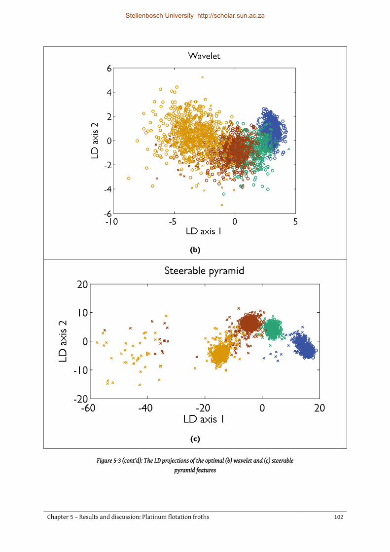
Chapter 5 – Results and discussion: Platinum flotation froths 102
(b)
(c)
Figure 5-3 (cont’d): The LD projections of the optimal (b) wavelet and (c) steerable pyramid features
Stellenbosch University http://scholar.sun.ac.za

Chapter 5 – Results and discussion: Platinum flotation froths 103
(d)
(e)
Figure 5-3 (cont’d): The LD projections of the optimal (d) texton and (e) LBP features.
Stellenbosch University http://scholar.sun.ac.za
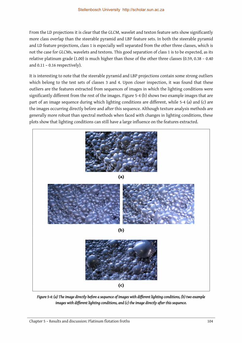
Chapter 5 – Results and discussion: Platinum flotation froths 104
From the LD projections it is clear that the GLCM, wavelet and texton feature sets show significantly more class overlap than the steerable pyramid and LBP feature sets. In both the steerable pyramid and LD feature projections, class 1 is especially well separated from the other three classes, which is not the case for GLCMs, wavelets and textons. This good separation of class 1 is to be expected, as its relative platinum grade (1.00) is much higher than those of the other three classes (0.59, 0.38 – 0.40 and 0.11 – 0.16 respectively).
It is interesting to note that the steerable pyramid and LBP projections contain some strong outliers which belong to the test sets of classes 3 and 4. Upon closer inspection, it was found that these outliers are the features extracted from sequences of images in which the lighting conditions were significantly different from the rest of the images. Figure 5-4 (b) shows two example images that are part of an image sequence during which lighting conditions are different, while 5-4 (a) and (c) are the images occurring directly before and after this sequence. Although texture analysis methods are generally more robust than spectral methods when faced with changes in lighting conditions, these plots show that lighting conditions can still have a large influence on the features extracted.
(a)
(b)
(c)
Figure 5-4: (a) The image directly before a sequence of images with different lighting conditions, (b) two example images with different lighting conditions, and (c) the image directly after this sequence.
Stellenbosch University http://scholar.sun.ac.za

Chapter 5 – Results and discussion: Platinum flotation froths 105
5.5 Computer running times
5.5.1 Training The computation times required to train and test the various image analysis methods are an important consideration. If the training of a model is very slow, it may not be feasible to use in cases where frequent recalibration is required. Additionally, with slow training it may not be possible to fully optimise the algorithm by testing all feasible hyperparameter combinations, or repetitions of the experiment will be limited.
The running times required to train each feature set and classifier combination, on a computer with an Intel® Core™ i7-2600 CPU (quad-core @ 3.40 GHz frequency) and 16 GB RAM, are reported in table 5-5.
Table 5-5: Computation times for the training of each model
For each feature extraction method, this table shows the number of hyperparameter combinations that were tested and the average time taken to extract a feature set for a single hyperparameter combination (ℋ𝐹), in minutes. The total training times for all hyperparameter combinations, including the time taken to train the classifiers and classify the validation data to optimise the classification hyperparameters for K-NN and DA, are shown in the last two columns.
All feature extraction methods, with the exception of textons, have reasonable training times, requiring between 5 minutes (wavelets) and 77 minutes (steerable pyramids) to extract the features for one hyperparameter combination. The texton algorithm is by far the slowest, taking 1077 minutes (18 hours) on average to compute the texton features for a single set of feature extraction hyperparameters. The reasons why texton features require long computer running times to be computed are explained in more detail in section 4.5.4 (p. 84) in the chapter on materials and methods.
Despite the high computational complexity of the texton algorithm, the use of texton features would still be merited if they lead to exceptionally good classification performance. However, for this case study it was not clear if textons outperform any of the other methods significantly, as the classification error when using K-NN was very high, while the error when using DA was very low. The use of texton features is therefore not recommended for this case study.
Method Number of ℋ𝐹
Training time per ℋ𝐹 (min)
Total training time for feature extraction and classification (h)
K-NN DA GLCM 15 27 6.8 6.8 Wavelet 3 5 0.3 0.3 Steerable pyramid 4 77 5.2 5.1 Texton 6 1077 106 108 LBP 12 11 2.3 2.3
Stellenbosch University http://scholar.sun.ac.za

Chapter 5 – Results and discussion: Platinum flotation froths 106
5.5.2 Testing The time taken to test one image is equivalent to the measurement delay that would be expected when using the method in an inferential sensor for online prediction. If the measurement delay is comparable to the time constant of the system, the sensor would not be very useful, since the measured process variables could change as fast as they are being measured.
The running times required to test each feature set and classifier combination, on the same computer as mentioned previously in this section, are reported in table 5-6.
Table 5-6: Computation times for the testing of each method combination
From this table it can be seen that the longest running time required to classify a single test image is 2.77 seconds for the steerable pyramid and K-NN method combination. This is deemed acceptable, since computation times in the order of seconds would certainly not be in a range comparable to the time constant of an industrial milling or grinding system with a hydrocyclone separator.
Note that while the texton features were slow to compute during training, testing with texton features is fast. This is because the slow clustering step does not have to be repeated during testing.
5.6 Conclusions Two of the three advanced texture analysis methods, namely steerable pyramids and LBPs, led to much improved classification results compared to the baseline methods (GLCMs and wavelets). However, the use of the texton feature set did not show any improvement.
DA generally outperforms K-NN, and overall the best method combination was steerable pyramids with a LDA classifier leading to 11.1% classification error. This is a significant improvement over the best classifier with GLCM features (11-NN with an error rate of 35.2%) and the best classifier with wavelet features (QDA with an error rate of 27.1%). It can therefore be concluded that some advanced texture feature extraction methods can improve the performance of a vision-based inferential sensor for this froth flotation application.
Poor test results when compared to validation results show that, while some of the feature extraction methods may perform well when the process conditions are similar to those of training
Method Time to test one image by extracting
features and classifying (s) K-NN DA
GLCM 0.52 0.51 Wavelet 0.20 0.19 Steerable pyramid 2.77 2.01 Texton 0.44 0.45 LBP 0.36 0.37
Stellenbosch University http://scholar.sun.ac.za

Chapter 5 – Results and discussion: Platinum flotation froths 107
data, there is a problem with extensibility to unseen data. Further investigation showed that the probability distribution estimate of the test set was very different from that of the training set, possibly indicating that the steady state assumption was false, or that a wide variety of froth appearances may occur at a single steady state. If the latter, it may be difficult to determine the grade of a platinum flotation froth from its visual appearance alone. While there certainly seems to be a correlation between froth appearance and froth grade, results might be improved by using such visual features in conjunction with other process data.
To determine whether the prediction of the platinum grade in flotation froths from visual information is viable, it is recommended that a more extensive set of training data, covering a wide range of operating conditions and process states, is collected.
Stellenbosch University http://scholar.sun.ac.za

Chapter 6 Results and discussion: Coal on a conveyor belt
The prediction of fines fraction classes from images of coal on a conveyor belt was considered in this case study. The results showed that the wavelet, steerable pyramid, texton and LBP methods significantly outperformed GLCMs.
Stellenbosch University http://scholar.sun.ac.za

Chapter 6 – Results and discussion: Coal on a conveyor belt 109
6.1 Introduction In this case study, the estimation of the fraction of fine particles in coal on a conveyor belt is considered. A total of 280 images of particulate coal on a laboratory scale conveyor belt, grouped into three fines fraction classes, were collected as described in section 0 (p. 67). Features were extracted from the images using five texture analysis methods and the quality of each feature set was assessed by determining its classification performance with two classifiers.
A random 75% of the data in each class was used for training and cross-validation, with the remaining 25% being reserved to test the best feature set for each feature extraction method (as determined by cross-validation). The number of images in each class is shown in table 6-1.
Table 6-1: Sizes of training and test sets in coal data set
Since images were randomly partitioned into training and test sets, it was possible to repeat the entire image analysis workflow with a different random partitioning each time. The entire experimental procedure, for all feature sets except texton features, was repeated ten times so that a sensitivity analysis on the error rates could be performed. The texton feature extraction could not be repeated ten times due to the exceptionally long computer running time that would be required to do so, the reasons for which are explained in more detail in section 4.5.4 (p. 84) in the chapter on materials and methods.
The remainder of this chapter is organised as follows. In section 6.2 the average test results across all ten runs are reported, a sensitivity analysis is performed and the significance of the results is discussed. A more in-depth analysis is then performed in section 6.3, based mostly on one run only, by investigating several further aspects. This includes linear discriminant (LD) projections of the feature sets, a discussion on the optimal hyperparameters and computer running times for all algorithms. Final conclusions are drawn in section 6.4.
6.2 Classification results The mean test error percentages for each feature set and classification method, averaged across all ten runs (except for textons, which had only one run), are given in table 6-2 and portrayed visually in figure 6-1. These error rates were obtained upon classification of the 70 test images into three fines fraction classes. The cross-validation error rates and standard deviations, averaged across all
Class Number of images
Training Test Total 1: Coarse 60 (12 per fold) 20 80 2: Intermediate 90 (18 per fold) 30 120 3: Fine 60 (12 per fold) 20 80
Totals: 210 70 280
Stellenbosch University http://scholar.sun.ac.za

Chapter 6 – Results and discussion: Coal on a conveyor belt 110
ten runs, are reported in table 6-3. The full validation and test results for all ten runs may be found in Appendix C.
Table 6-2: Averages and confidence intervals of test error percentages across all ten runs for all feature sets and classification methods
Table 6-3: Averages and standard deviations of validation error rates during five-fold cross-validation,
averaged across all ten runs
Method K-NN DA
Avg. 95% confidence Avg. 95% confidence GLCM 25.6% ±3.7% 17.0% ±3.2% Wavelet 14.7% ±2.6% 13.3% ±2.6% Steerable pyramid 13.0% ±3.1% 12.0% ±4.4% Texton (only 1 run) 8.6% N/A 10.0% N/A LBP 15.1% ±3.6% 10.3% ±2.3%
Method K-NN DA
Avg. Std. Avg. Std. GLCM 22.0% 4.8% 16.2% 5.3% Wavelet 12.9% 5.8% 12.8% 5.6% Steerable pyramid 11.7% 4.0% 9.4% 3.9% Texton (only 1 run) 3.8% 2.1% 5.7% 2.7% LBP 13.0% 4.8% 8.2% 3.7%
Figure 6-1: Average error rates for each feature extraction and classification method. The error bars indicate 95% confidence intervals for the error rates.
0%
5%
10%
15%
20%
25%
30%
35%
GLCM Wavelet Steerable
pyramid
Texton LBP
Err
or
perc
en
tage
K-NN
DA
Stellenbosch University http://scholar.sun.ac.za

Chapter 6 – Results and discussion: Coal on a conveyor belt 111
6.2.1 Sensitivity analysis Table 6-4 shows the results of a two-factor ANOVA that was performed to determine the significance of the effect that two factors, the feature set and the classifier, have on the error rate. The texton results were not used in this analysis, since there was only run using this feature set and this could seriously bias the results.
Table 6-4: Two-factor ANOVA results for the factors “feature set” and “classifier”
It can be deduced from these ANOVA results that all factors are significant at a 95% confidence level (𝛼 = 0.05): the choice of feature set, classifier and interaction between the two factors. For the feature sets, this means that the error rates obtained with at least two feature sets differ significantly.
To determine which feature sets are significantly different from one another, a Bonferroni post-hoc test was performed. It was decided in advance that the test will only be done between all pairs of feature sets excluding textons (6 tests) and not between the eight feature set and classifier combinations (28 tests), since the focus of this work is on texture feature extraction. The results for the Bonferroni post-hoc test are reported in table 6-5, where the p-values that are significant at a 95% confidence level are marked in green.
Table 6-5: Bonferroni post-hoc test p-values for pair-wise comparisons between all feature sets
6.2.2 Discussion
Feature extraction methods The Bonferroni test results in table 6-5 indicate that the mean error rate obtained by using GLCM features differed significantly from the error rates obtained by all other feature extraction methods, as p = 0.0000 in all of these cases. No statistically significant distinction could be drawn between any of the other three feature extraction methods. This is in line with what would be expected when visually inspecting the mean error rates and 95% confidence intervals plotted in figure 6-1. It
Effect SS DOF MS F p Feature set 0.104 3 0.035 16.65 0.000 Classifier 0.031 1 0.031 15.12 0.000 Feature set*Classifier 0.019 3 0.006 2.99 0.037
Feature set {1} (.21286)
{2} (.14000)
{3} (.12500)
{5} (.12714)
1 GLCM 0.0000 0.0000 0.0000 2 Wavelet 0.0000 1.0000 1.0000 3 Steerable pyramid 0.0000 1.0000 1.0000 5 LBP 0.0000 1.0000 1.0000
Stellenbosch University http://scholar.sun.ac.za

Chapter 6 – Results and discussion: Coal on a conveyor belt 112
appears as though the GLCM and K-NN combination led to a significantly higher error rate than all of the other methods, and that the GLCM and DA combination led to a significantly higher error rate than the LBP and DA combination.
From the test results it is apparent that textons also significantly outperformed GLCMs, although the results are expected to be biased in favour of textons: textons had only one run, and this run had good results. Nonetheless, this is the best conclusion that can be made in the absence of more information.
In summary, it can be concluded from these results that the advanced textural feature extraction methods (steerable pyramids, textons and LBPs) outperformed the baseline GLCM method, but not the wavelet method. The baseline wavelet method was on par with the advanced methods.
Classifiers DA outperforms K-NN for every feature set except textons, and according to the ANOVA results in table 6-4, this outperformance is significant at a 95% confidence level. On average, DA outperforms K-NN by 2.9%, which is not as large a difference as the 8.3% outperformance that was observed for the flotation case study.
A likely explanation for the better performance of DA is that the numbers of samples in each class are not equal: 29% of the images belong to class 1, 43% to class 2 and 29% to class 3. While K-NN is biased towards the classes containing more data points, DA takes the prior probabilities into account when training the classification model. The data distribution between classes is not as skewed as in the flotation case study, so for this case study DA is not expected to outperform K-NN by as large a margin as in the flotation case study, which is indeed the case.
Comparison between validation and test results It is expected that validation results would be slightly optimistic compared to test results on unseen data, since the validation results reported in table 6-3 are the lowest error percentages for each method, as obtained with the best hyperparameter combination. A large discrepancy between the validation and test error rates could be an indication of overfitting.
In this case, the average validation error rates were not drastically lower than the average test error rates – 2.0% lower on average. It can therefore be concluded that that overfitting has not occurred.
6.3 Further analysis A more in-depth analysis of the experiment and its results was carried out by considering run 1 in more detail. The choice of run 1 is arbitrary, since the data was divided randomly into training and test sets for each run.
Several aspects are investigated in this section. First, the discriminability of the feature sets are visually examined by projecting each feature set onto its linear discriminant (LD) axes. The classification results from run 1 are then reported and contrasted against the average results across
Stellenbosch University http://scholar.sun.ac.za

Chapter 6 – Results and discussion: Coal on a conveyor belt 113
all ten runs, and the optimal hyperparameters for this run are discussed. Finally, the computer running times for training and testing are reported.
6.3.1 LD projection As a visual indication of the separation achieved with each feature set, the optimal feature sets when using discriminant analysis, for run 1, were projected onto the first two linear discriminant (LD) axes. These projections are shown in figure 6-2 (a) to (e).
(a)
Figure 6-2 (a): The LD projection of the optimal GLCM features
Stellenbosch University http://scholar.sun.ac.za

Chapter 6 – Results and discussion: Coal on a conveyor belt 114
(b)
(c)
Figure 6-2 (cont’d): The LD projections of the optimal (b) wavelet and (c) steerable pyramid features
Stellenbosch University http://scholar.sun.ac.za

Chapter 6 – Results and discussion: Coal on a conveyor belt 115
(d)
(e)
Figure 6-2 (cont’d): The LD projections of the optimal (d) texton and (e) LBP features.
Stellenbosch University http://scholar.sun.ac.za
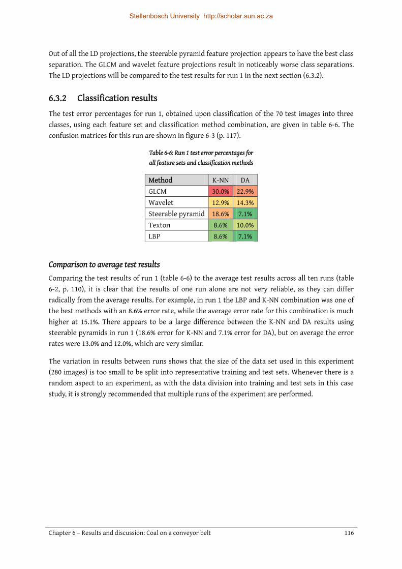
Chapter 6 – Results and discussion: Coal on a conveyor belt 116
Out of all the LD projections, the steerable pyramid feature projection appears to have the best class separation. The GLCM and wavelet feature projections result in noticeably worse class separations. The LD projections will be compared to the test results for run 1 in the next section (6.3.2).
6.3.2 Classification results The test error percentages for run 1, obtained upon classification of the 70 test images into three classes, using each feature set and classification method combination, are given in table 6-6. The confusion matrices for this run are shown in figure 6-3 (p. 117).
Table 6-6: Run 1 test error percentages for all feature sets and classification methods
Comparison to average test results Comparing the test results of run 1 (table 6-6) to the average test results across all ten runs (table 6-2, p. 110), it is clear that the results of one run alone are not very reliable, as they can differ radically from the average results. For example, in run 1 the LBP and K-NN combination was one of the best methods with an 8.6% error rate, while the average error rate for this combination is much higher at 15.1%. There appears to be a large difference between the K-NN and DA results using steerable pyramids in run 1 (18.6% error for K-NN and 7.1% error for DA), but on average the error rates were 13.0% and 12.0%, which are very similar.
The variation in results between runs shows that the size of the data set used in this experiment (280 images) is too small to be split into representative training and test sets. Whenever there is a random aspect to an experiment, as with the data division into training and test sets in this case study, it is strongly recommended that multiple runs of the experiment are performed.
Method K-NN DA GLCM 30.0% 22.9% Wavelet 12.9% 14.3% Steerable pyramid 18.6% 7.1% Texton 8.6% 10.0% LBP 8.6% 7.1%
Stellenbosch University http://scholar.sun.ac.za

Chapter 6 – Results and discussion: Coal on a conveyor belt 117
Figure 6-3: Run 1 confusion matrices for all feature extraction and classification combinations
1 2 3 1 2 3
1 60.0 40.0 0.0 1 70.0 30.0 0.0
2 23.3 70.0 6.7 2 13.3 76.7 10.0
3 0.0 20.0 80.0 3 0.0 15.0 85.0
1 2 3 1 2 3
1 80.0 20.0 0.0 1 85.0 15.0 0.0
2 3.3 86.7 10.0 2 6.7 86.7 6.7
3 0.0 5.0 95.0 3 0.0 15.0 85.0
1 2 3 1 2 3
1 75.0 25.0 0.0 1 95.0 5.0 0.0
2 13.3 73.3 13.3 2 3.3 93.3 3.3
3 0.0 0.0 100 3 0.0 10.0 90.0
1 2 3 1 2 3
1 90.0 10.0 0.0 1 95.0 5.0 0.0
2 0.0 90.0 10.0 2 3.3 86.7 10.0
3 0.0 5.0 95.0 3 0.0 10.0 90.0
1 2 3 1 2 3
1 90.0 10.0 0.0 1 95.0 5.0 0.0
2 0.0 96.7 3.3 2 3.3 90.0 6.7
3 0.0 15.0 85.0 3 0.0 5.0 95.0
K-NN DA
GLCM
Predicted classes Predicted classes
Act
ua
l cl
ass
es
Act
ua
l cl
ass
es
Wavelet
Predicted classes Predicted classes
Act
ua
l cl
ass
es
Act
ua
l cl
ass
es
Steerable
pyramid
Predicted classes Predicted classes
Act
ua
l cl
ass
es
Act
ua
l cl
ass
es
Texton
Predicted classes Predicted classes
Act
ua
l cl
ass
es
Act
ua
l cl
ass
es
LBP
Predicted classes Predicted classes
Act
ua
l cl
ass
es
Act
ua
l cl
ass
es
Stellenbosch University http://scholar.sun.ac.za

Chapter 6 – Results and discussion: Coal on a conveyor belt 118
Confusion matrices The test results for run 1 showed that GLCMs with both K-NN and DA classifiers, and steerable pyramids with a K-NN classifier, were the three worst methods. This is affirmed by looking at the confusion matrices for this run (figure 6-3), where the sensitivity and specificity of these three methods appear to be noticeably worse. For the remaining seven method combinations, all classes are relatively well classified, and there does not appear to be a bias towards a particular class. No images from class 1 were incorrectly classified into class 3, and no images from class 3 were incorrectly classified into class 1, for any of the ten method combinations.
Comparison to LD projections The test results for DA in table 6-6 are in line with what would be expected upon investigation of the LD projections for each feature set (figure 6-2, p. 113). The most overlap between classes is found in the GLCM feature projection, followed by the wavelet feature projection, and these methods have the highest and second-highest error rates (22.9% and 14.3%, respectively). The steerable pyramid features result in especially well separated clusters, and this method did have the lowest error rate (along with LBPs).
6.3.3 Hyperparameters The hyperparameters that led to the validation results for run 1 are reported in table 6-7. The optimal hyperparameters found for all ten runs are included in Appendix C.
Table 6-7: Optimal hyperparameter settings and dimensionalities of feature sets for run 1
For the GLCM features, the optimal number of grey levels when using K-NN and DA classifiers were 𝐺 = 32 and 𝐺 = 64, respectively. This is a significant result, since in practice this hyperparameter is usually not optimised, but rather fixed at 𝐺 = 8 as originally proposed by Haralick (1979).
Method K-NN DA
Feature extraction hyperparameters ℋ𝐹
Feature set size 𝐾𝑁
Feature extraction hyperparameters ℋ𝐹
Feature set size
Type
GLCM 𝐺 = 32 𝐷 = 3
PCA: 𝑣𝑎𝑟 = 99% 4 11
𝐺 = 64 𝐷 = 3
PCA = 𝑛𝑜𝑛𝑒 8 𝐿𝑖𝑛𝑒𝑎𝑟
Wavelet Type = ‘ℎ𝑎𝑎𝑟’ PCA = 𝑛𝑜𝑛𝑒 18 6 Type =′ ℎ𝑎𝑎𝑟′
PCA: 𝑣𝑎𝑟 = 99% 9 𝐿𝑖𝑛𝑒𝑎𝑟
Steerable pyramid
𝑆𝑖𝑛𝑐 = 6 𝑊 = 7
PCA: 𝑣𝑎𝑟 = 95% 29 4
𝑆𝑖𝑛𝑐 = 4 𝑊 = 11
PCA: 𝑣𝑎𝑟 = 95% 37 𝐿𝑖𝑛𝑒𝑎𝑟
Texton 𝐾𝑇 = 40 𝐹𝑆 = 25
PCA = 𝑛𝑜𝑛𝑒 40 5
𝐾𝑇 = 40 𝐹𝑆 = 25
PCA: 𝑣𝑎𝑟 = 95% 10 𝑄𝑢𝑎𝑑𝑟𝑎𝑡𝑖𝑐
LBP 𝑅 = 4 𝑃 = 16
Mapping = ′𝑟𝑖𝑢2′ PCA: 𝑣𝑎𝑟 = 99%
7 8 𝑅 = 2.5 𝑃 = 12
Mapping = ′𝑟𝑖𝑢2′ PCA = 𝑛𝑜𝑛𝑒
14 𝐿𝑖𝑛𝑒𝑎𝑟
Stellenbosch University http://scholar.sun.ac.za

Chapter 6 – Results and discussion: Coal on a conveyor belt 119
In the computation of the texton feature set, a smaller filter support size of 𝐹𝑆 = 25 was optimal, instead of the 𝐹𝑆 = 49 that was originally proposed by Schmid (2001) and used in all subsequent studies that were found in literature (see for example Varma & Zisserman, 2005; Jemwa & Aldrich, 2012).
It is interesting to note that the best type of DA was LDA for four out of the five texture feature sets, with only textons performing better when using a QDA classifier.
Two properties of texture analysis algorithms that are believed to play a large role in their performance are rotation and translation invariance as well as multiscale representation. In this case study it seems as though rotation invariance were important algorithm properties: the optimal mapping type for LBPs was rotation invariant and this feature set was overall one of the best feature sets. Textons, which are also entirely rotation invariant in this implementation, also showed good performance.
Multiscale representation also seems to have been important in this case study. The only advanced property of the wavelet texture analysis algorithm is that it results in a multiscale representation, and the wavelet feature set performed surprisingly well in this case study. Steerable pyramids are also multiscale representations, and features extracted from these representations also led to very low error rates.
6.3.4 Computer running times
Training The computation times required to train and test the various image analysis methods are an important consideration. If the training of a model is very slow, it may not be feasible to use in cases where frequent recalibration is required. Additionally, with slow training it may not be possible to fully optimise the algorithm by testing all feasible hyperparameter combinations, or repetitions of the experiment will be limited.
The running times required to train each feature set and classifier combination, on a computer with an Intel® Core™ i7-2600 CPU (quad-core @ 3.40 GHz frequency) and 16 GB RAM, are reported in table 6-8.
Table 6-8: Computation times for the training of each model
Method Number of ℋ𝐹
Training time per ℋ𝐹 (min)
Total training time for feature extraction and classification (h)
K-NN DA GLCM 15 2.1 0.64 0.61 Wavelet 3 0.4 0.05 0.04 Steerable pyramid 4 7.4 0.53 0.52 Texton 6 1008 103 99 LBP 12 1.3 0.37 0.34
Stellenbosch University http://scholar.sun.ac.za

Chapter 6 – Results and discussion: Coal on a conveyor belt 120
For each feature extraction method, this table shows the number of hyperparameter combinations that were tested and the average time taken to extract a feature set for a single hyperparameter combination (ℋ𝐹), in minutes. The total training times for all hyperparameter combinations, including the time taken to train the classifiers and classify the validation data to optimise the classification hyperparameters for K-NN and DA, are shown in the last two columns.
All feature extraction methods, with the exception of textons, have reasonable training times, requiring between 0.4 minutes (wavelets) and 7.4 minutes (steerable pyramids) to extract the features for one hyperparameter combination. The texton algorithm is by far the slowest, taking 1008 minutes (17 hours) on average to compute the texton features for a single set of feature extraction hyperparameters. The reasons why texton feature extraction is slow are explained in more detail in section 4.5.4 (p. 84) in the chapter on materials and methods.
Despite the high computational complexity of the texton algorithm, the use of texton features would still be merited if they lead to exceptionally good classification performance. However, in this case study texton features did not perform well, and are therefore not recommended for this case study.
Testing The time taken to test one image is equivalent to the measurement delay that would be expected when using the method in an inferential sensor for online prediction. If the measurement delay is comparable to the time constant of the system, the sensor would not be very useful, since the measured process variables could change as fast as they are being measured.
The running times required to test each feature set and classifier combination, on the same computer as mentioned previously in this section, are reported in table 6-9.
Table 6-9: Computation times for the testing of each method combination
From table 6-9 it can be seen that the longest running time required to classify a single test image is 2.12 seconds for steerable pyramids. This is deemed acceptable, since computation times in the order of seconds would certainly not be in a range comparable to the time constant of an industrial system fed with coal from a conveyor belt.
Method Time to test one image by extracting
features and classifying (s) K-NN DA
GLCM 0.36 0.35 Wavelet 0.12 0.12 Steerable pyramid 2.12 2.12 Texton 0.30 0.30 LBP 0.40 0.37
Stellenbosch University http://scholar.sun.ac.za
Chapter 6 – Results and discussion: Coal on a conveyor belt 121
Note that while the texton features were slow to compute during training, testing with texton features is fast. This is because the slow clustering step does not have to be repeated during testing.
6.4 Conclusions In this case study the three advanced texture analysis methods, as well as wavelets, led to significantly better classification results than the baseline GLCM method. A statistically significant distinction between the performance of each of the three advanced texture analysis methods and wavelets could not be made. DA slightly outperformed K-NN for all feature sets except textons.
It is unlikely that the four better methods truly have the same performance on this data set, and it is therefore concluded that more data would be needed to be able to determine the best feature extraction method.
The best test result obtained was with the texton and K-NN combination, which gave an 8.1% error. In general, the error rates were around 10%. Although this may seem like relatively good performance, one has to remember that this error rate was obtained upon classification into three very broad classes. In practise, the fines fractions of interest is in a much narrower range of 0 – 10% fines, which means that much more precise discrimination is required. The textural features used in this work could be used as input to a regression model to determine if such precise prediction is possible. Based on the results obtained in this work, it is not expected that the approach would be able to discriminate between fines fractions that are in the narrow range of 0 – 10%.
Stellenbosch University http://scholar.sun.ac.za

Chapter 7 Results and discussion: Hydrocyclone underflows
The prediction of mean particle size classes from images of hydrocyclone underflows was considered in this case study. The results showed that the steerable pyramid and LBP methods significantly outperformed the GLCM and wavelet methods. The result for textons was inconclusive.
Stellenbosch University http://scholar.sun.ac.za
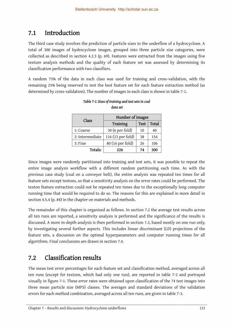
Chapter 7 – Results and discussion: Hydrocyclone underflows 123
7.1 Introduction The third case study involves the prediction of particle sizes in the underflow of a hydrocyclone. A total of 300 images of hydrocyclone images, grouped into three particle size categories, were collected as described in section 4.2.3 (p. 69). Features were extracted from the images using five texture analysis methods and the quality of each feature set was assessed by determining its classification performance with two classifiers.
A random 75% of the data in each class was used for training and cross-validation, with the remaining 25% being reserved to test the best feature set for each feature extraction method (as determined by cross-validation). The number of images in each class is shown in table 7-1.
Table 7-1: Sizes of training and test sets in coal data set
Since images were randomly partitioned into training and test sets, it was possible to repeat the entire image analysis workflow with a different random partitioning each time. As with the previous case study (coal on a conveyor belt), the entire analysis was repeated ten times for all feature sets except textons, so that a sensitivity analysis on the error rates could be performed. The texton feature extraction could not be repeated ten times due to the exceptionally long computer running time that would be required to do so. The reasons for this are explained in more detail in section 4.5.4 (p. 84) in the chapter on materials and methods.
The remainder of this chapter is organised as follows. In section 7.2 the average test results across all ten runs are reported, a sensitivity analysis is performed and the significance of the results is discussed. A more in-depth analysis is then performed in section 7.3, based mostly on one run only, by investigating several further aspects. This includes linear discriminant (LD) projections of the feature sets, a discussion on the optimal hyperparameters and computer running times for all algorithms. Final conclusions are drawn in section 7.4.
7.2 Classification results The mean test error percentages for each feature set and classification method, averaged across all ten runs (except for textons, which had only one run), are reported in table 7-2 and portrayed visually in figure 7-1. These error rates were obtained upon classification of the 74 test images into three mean particle size (MPS) classes. The averages and standard deviations of the validation errors for each method combination, averaged across all ten runs, are given in table 7-3.
Class Number of images
Training Test Total 1: Coarse 30 (6 per fold) 10 40 2: Intermediate 116 (23 per fold) 38 154 3: Fine 80 (16 per fold) 26 106
Totals: 226 74 300
Stellenbosch University http://scholar.sun.ac.za

Chapter 7 – Results and discussion: Hydrocyclone underflows 124
The full validation and test results for all ten runs may be found in Appendix D.
Table 7-2: Average and standard deviation test error percentages across all ten runs for all feature sets and classification methods
Method K-NN DA
Avg. 95% confidence Avg. 95% confidence GLCM 14.2% 2.8% 13.5% 2.2% Wavelet 13.0% 1.8% 12.3% 3.2% Steerable pyramid 10.7% 2.8% 7.8% 1.9% Texton (only 1 run) 16.2% N/A 6.8% N/A LBP 10.4% 1.8% 9.3% 1.9%
Table 7-3: Averages and standard deviations of validation error rates during five-fold cross-validation,
averaged across all ten runs
Method K-NN DA
Avg. Std. Avg. Std. GLCM 13.2% 4.9% 10.5% 4.7% Wavelet 11.7% 4.4% 10.9% 4.8% Steerable pyramid 8.5% 4.8% 6.9% 3.7% Texton (only 1 run) 9.3% 4.8% 8.4% 3.5% LBP 11.0% 4.8% 8.3% 3.5%
Figure 7-1: Average error rates for each feature extraction and classification method. The error bars indicate 95% confidence intervals for the error rates.
0%
2%
4%
6%
8%
10%
12%
14%
16%
18%
GLCM Wavelet Steerable
pyramid
Texton LBP
Err
or
perc
en
tage
K-NN
DA
Stellenbosch University http://scholar.sun.ac.za

Chapter 7 – Results and discussion: Hydrocyclone underflows 125
7.2.1 Sensitivity analysis Table 7-4 shows the results of a two-factor ANOVA that was performed to determine the significance of the effect that two factors, the feature set and the classifier, have on the error rate. The texton results were not used in this analysis, since there was only run using this feature set and this could seriously bias the results.
Table 7-4: Two-factor ANOVA results for the factors “feature set” and “classifier”
These ANOVA results show that only the choice of feature set is significant at a 95% confidence level (𝛼 = 0.05). While the choice of classifier is not significant at this confidence level, its p-value is still below the 90% confidence level threshold. Given that this ANOVA was based on only ten repetitions factor combination, the significance of the choice of classifier should not be entirely disregarded. The interaction between the two factors is not significant, which means that the error rates obtained with both K-NN and DA follow the same trend across the various feature sets (this is also apparent from figure 7-1 when disregarding the texton results).
To determine which feature sets are significantly different from one another, a Bonferroni post-hoc test was performed. It was decided in advance that the test will only be done between all pairs of feature sets excluding textons (6 tests) and not between the eight feature set and classifier combinations (28 tests), since the focus of this work is on texture feature extraction. The results for the Bonferroni post-hoc test are reported in table 7-5, where the p-values that are significant at a 95% confidence level are marked in green.
Table 7-5: Bonferroni post-hoc test p-values for pair-wise comparisons between all feature sets
7.2.2 Discussion
Feature extraction methods The Bonferroni test results in table 7-5 show that the steerable pyramid feature set significantly outperformed both of the baseline methods, GLCMs and wavelets. The LBP features also
Effect SS DOF MS F p Feature set 0.029 3 0.010 8.869 0.000 Classifier 0.003 1 0.003 3.189 0.078 Feature set*Classifier 0.002 3 0.001 0.488 0.691
Feature extraction {1} (.13851)
{2} (.12635)
{3} (.09257)
{5} (.09865)
1 GLCM 1.0000 0.0002 0.0017 2 Wavelet 1.0000 0.0109 0.0586 3 Steerable pyramid 0.0002 0.0109 1.0000 5 LBP 0.0017 0.0586 1.0000
Stellenbosch University http://scholar.sun.ac.za

Chapter 7 – Results and discussion: Hydrocyclone underflows 126
outperformed the GLCM features, but not the wavelet features at a 95% confidence level. However, as the p-value for the LBP-wavelet test is p = 0.0586, the difference in performance is still significant with 90% confidence, so the possibility of a significant difference between these two methods should not be discounted.
These post-hoc test results are in line with what would be expected when visually inspecting the mean error rates and 95% confidence intervals plotted in figure 7-1. It appears as though two of the method combinations were significantly better than three others: steerable pyramids with a DA classifier were better than GLCMs with any classifier, and better than wavelets with a K-NN classifier. LBPs with a DA classifier also appear to be significantly better than those three method combinations.
Texton features combined with a K-NN classifier resulted in the highest error rate of all methods (16.2%), but with a DA classifier led to the lowest error rate of all methods (6.8%). It is therefore not clear whether textons showed better or worse performance than the other feature sets, especially when taking into account that only one texton run was performed.
In summary, it can be concluded that two of the three advanced textural feature extraction methods, steerable pyramids and LBPs, outperformed the baseline GLCM and wavelet methods.
Classifiers DA outperforms K-NN for every feature set, although not significantly so at a 95% confidence level (according the ANOVA results). It should be noted here that the texton results were not used in the ANOVA, and for textons the DA classifier was much better than the K-NN classifier. However, it is quite possible that the average test result for textons over ten runs would not show such a large discrepancy between classification with K-NN and DA.
On average, DA outperforms K-NN by 2.9%, although this includes the texton result, which has a large influence on this average outperformance. A possible explanation for the improved performance of DA is that the numbers of images in each class are very different: only 14% of the images belong to class 1, while 51% are in class 2 and 35% in class 3. While K-NN is biased towards the classes containing more data points, DA takes the prior probabilities into account when training the classification model.
Comparison between validation and test results It is expected that validation results would be slightly optimistic compared to test results on unseen data, since the validation results reported in Table 7-3 are the lowest error percentages for each method, as obtained with the best hyperparameter combination. A large discrepancy between the validation and test error rates could be an indication of overfitting.
The average validation error rates for each method, across all ten runs, were very close to the test error rates. The validation errors were only 0.9% lower on average. It can therefore be concluded that overfitting has not occurred.
Stellenbosch University http://scholar.sun.ac.za

Chapter 7 – Results and discussion: Hydrocyclone underflows 127
7.3 Further analysis A more in-depth analysis of the experiment and its results was carried out by considering run 1 in more detail. The choice of run 1 is arbitrary, since the data was divided randomly into training and test sets for each run.
Several aspects are investigated in this section. First, the discriminability of the feature sets are visually examined by projecting each feature set onto its linear discriminant (LD) axes. The classification results from run 1 are then reported and contrasted against the average results across all ten runs, and the optimal hyperparameters for this run are discussed. Finally, the computer running times for training and testing are reported.
7.3.1 LD projection As a visual indication of the separation achieved with each feature set, the optimal feature sets when using discriminant analysis, for run 1, were projected onto the first two linear discriminant (LD) axes. These projections are shown in figure 7-2 (a) to (e).
Stellenbosch University http://scholar.sun.ac.za

Chapter 7 – Results and discussion: Hydrocyclone underflows 128
(a)
Figure 7-2 (a): The LD projection of the optimal GLCM features
Stellenbosch University http://scholar.sun.ac.za

Chapter 7 – Results and discussion: Hydrocyclone underflows 129
(b)
(c)
Figure 7-2 (cont’d): The LD projections of the optimal (b) wavelet and (c) steerable pyramid features
Stellenbosch University http://scholar.sun.ac.za

Chapter 7 – Results and discussion: Hydrocyclone underflows 130
(d)
(e)
Figure 7-2 (cont’d): The LD projections of the optimal (d) texton and (e) LBP features.
Stellenbosch University http://scholar.sun.ac.za

Chapter 7 – Results and discussion: Hydrocyclone underflows 131
The projections of the three advanced textural feature sets point towards better class separation than the GLCM and wavelet projections, and that of steerable pyramids in particular seems to be the best. In both the GLCM and wavelet projections, the clusters for class 1 and 3 are close to each other, which may lead to an undesirable classification of data points in class 1 into class 3, and vice versa. The LD projections will be compared to the test results for run 1 in the next section (7.3.2).
7.3.2 Classification results The test error percentages for run 1, obtained upon classification of the 74 test images into three classes, using each feature set and classification method combination, are given in table 7-6, with the respective confusion matrices in figure 7-3 (p. 132).
Table 7-6: Run 1 test error percentages for all feature sets and classification methods
Comparison to average test results Comparing the test results of run 1 (table 7-6) to the average test results across all ten runs (table 6-2, p. 110), it is clear that the results of one run alone are not very reliable, as they can differ radically from the average results. For example, from the run 1 results one would conclude that steerable pyramid features lead to relatively high error rates, but the average test results for steerable pyramids were 10.7% with a K-NN classifier and 7.8% with a DA classifier, placing steerable pyramids among the best methods. The wavelet and DA combination led to one of the lowest error rates during run 1 (only 6.8% error), but on average the error rate for this combination was 12.3%, making it one of the worst methods. As was seen in case study II, it is clear that conclusions regarding the best feature sets cannot be drawn based on the results of run 1 only.
Method K-NN DA GLCM 13.5% 13.5% Wavelet 12.2% 6.8% Steerable pyramid 14.9% 13.5% Texton 16.2% 6.8% LBP 13.5% 9.5%
Stellenbosch University http://scholar.sun.ac.za

Chapter 7 – Results and discussion: Hydrocyclone underflows 132
Figure 7-3: Run 1 confusion matrices for all feature extraction and classification combinations
1 2 3 1 2 3
1 80.0 20.0 0.0 1 70.0 20.0 10.0
2 0.0 94.7 5.3 2 2.6 92.1 5.3
3 11.5 11.5 76.9 3 3.8 11.5 84.6
1 2 3 1 2 3
1 90.0 10.0 0.0 1 60.0 40.0 0.0
2 10.5 84.2 5.3 2 2.6 97.4 0.0
3 0.0 7.7 92.3 3 0.0 0.0 100
1 2 3 1 2 3
1 70.0 10.0 20.0 1 60.0 40.0 0.0
2 7.9 86.8 5.3 2 0.0 97.4 2.6
3 0.0 11.5 88.5 3 0.0 19.2 80.8
1 2 3 1 2 3
1 30.0 70.0 0.0 1 80.0 20.0 0.0
2 0.0 97.4 2.6 2 0.0 100 0.0
3 0.0 15.4 84.6 3 3.8 7.7 88.5
1 2 3 1 2 3
1 70.0 20.0 10.0 1 80.0 20.0 0.0
2 0.0 94.7 5.3 2 2.6 97.4 0.0
3 3.8 15.4 80.8 3 0.0 15.4 84.6
LBP
Predicted classes Predicted classes
Act
ual
cla
sses
Act
ual
cla
sses
Texton
Predicted classes Predicted classes
Act
ual
cla
sses
Act
ual
cla
sses
Steerable
pyramid
Predicted classes Predicted classes
Act
ual
cla
sses
Act
ual
cla
sses
Wavelet
Predicted classes Predicted classes
Act
ual
cla
sses
Act
ual
cla
sses
K-NN DA
GLCM
Predicted classes Predicted classes
Act
ual
cla
sses
Act
ual
cla
sses
Stellenbosch University http://scholar.sun.ac.za

Chapter 7 – Results and discussion: Hydrocyclone underflows 133
Confusion matrices Looking at the top row in each confusion matrix, it can be seen that most of the methods were not able to classify class 1 correctly. This is probably because there were only ten test images in this class (13.5% of the test images). Most notably, with the texton and K-NN combination 30% of the images in class 1 were correctly classified into class 1, with 70% of the images being incorrectly classified into class 2. With several of the other method combinations, some of the class 1 images were even classified into class 3, and some class 3 images into class 1.
The challenges associated with the small size of class 1 is an indication that the data set is not very suited to classification, especially when using K-NN, which is biased towards classes that contain more data points. It would also not be sensible to redefine class 1 to contain some data from class 2, since there is a very large difference between the mean particle sizes of images in class 1 and those of images in class 2 (refer to the data discretisation as described in section 4.2.3, p. 69, in the chapter on materials and methods). In future work, regression instead of classification could be performed on the textural features to predict mean particle sizes.
Comparison to LD projections The test errors when using DA for run 1 were the lowest for the wavelet and texton feature sets (both 6.8%), followed by that of the LBP feature set (9.5%). Comparing these results to the LD projections from figure 7-2, the outcomes for wavelets and steerable pyramids are surprising. From the projections shown in figure 7-2 (b) and (c), it appears as though the classes obtained with steerable pyramid features would be more separable than those obtained with wavelet features. However, the test results for these feature sets with DA show the opposite.
Upon inspection of the confusion matrices of the wavelet features classified with DA and steerable pyramid features classified with DA, the major difference between the two is that 19.2% of the images in class 3 were incorrectly classified into class 2 (this amounts to five images) when using steerable pyramid features, while for wavelets all of the class 3 images were correctly classified. A possible reason for this unexpected result is that the separating line between two classes, as found by DA using training data, does not necessarily lie at the optimal separation between two classes when test data is included. The five images from class 3 that were incorrectly classified into class two are indicated in black on the LD projection in figure 7-4.
Stellenbosch University http://scholar.sun.ac.za

Chapter 7 – Results and discussion: Hydrocyclone underflows 134
Figure 7-4: LD projection of steerable pyramid features, where incorrectly classified test data points from class 3 marked with black stars
7.3.3 Optimal hyperparameters The hyperparameters that led to the validation results for run 1 are reported in table 7-7. The full validation and test results and optimal hyperparameter settings for all ten runs may be found in Appendix D.
Stellenbosch University http://scholar.sun.ac.za

Chapter 7 – Results and discussion: Hydrocyclone underflows 135
Table 7-7: Optimal hyperparameter settings and dimensionalities of feature sets for run 1
For the GLCM features, the optimal number of grey levels when using K-NN and DA classifiers were 𝐺 = 32 and 𝐺 = 64, respectively. This is a significant result, since in practice this hyperparameter is usually not optimised, but rather fixed at 𝐺 = 8 as originally proposed by Haralick (1979).
Another important result is that in computation of the texton feature set, a smaller filter support size of 𝐹𝑆 = 25 was optimal. In contrast, 𝐹𝑆 = 49 was originally proposed by Schmid (2001) and has been used in all subsequent studies that were found in literature (see for example Varma & Zisserman, 2005; Jemwa & Aldrich, 2012).
It is interesting to note that the best type of DA was LDA for four out of the five texture feature sets, with only GLCMs performing better with a QDA classifier.
Two properties of texture analysis algorithms that are believed to play a large role in their performance are rotation and translation invariance as well as multiscale representation. However, in this case study it seems as though rotation invariance was not an important indicator of performance. While the LBP feature set performed well, the optimal mapping type for this feature set was not rotation invariant. Also, steerable pyramids are rotation invariant only to some extent and also showed excellent performance.
Multiscale representation alone did not guarantee success in this case study: both the wavelet and steerable pyramid feature sets were extracted from multiscale representations, but only steerable pyramids performed well. It is suggested that the improved performance of the steerable pyramid feature set might instead be ascribed to the aptness of the advanced statistical features that are extracted from the representation.
Method
K-NN DA
Feature extraction hyperparameters ℋ𝐹
Feature set size 𝐾𝑁
Feature extraction hyperparameters ℋ𝐹
Feature set size Type
GLCM 𝐺 = 32 𝐷 = 5
PCA = 𝑛𝑜𝑛𝑒 8 4
𝐺 = 64 𝐷 = 5
PCA = 𝑛𝑜𝑛𝑒 8 𝑄𝑢𝑎𝑑𝑟𝑎𝑡𝑖𝑐
Wavelet Type = ‘𝑑𝑏3’ PCA = 𝑛𝑜𝑛𝑒 21 1 Type = ‘𝑠𝑦𝑚4’
PCA = 𝑛𝑜𝑛𝑒 21 𝐿𝑖𝑛𝑒𝑎𝑟
Steerable pyramid
𝑆𝑖𝑛𝑐 = 6 𝑊 = 11
PCA: 𝑣𝑎𝑟 = 95% 23 1
𝑆𝑖𝑛𝑐 = 4 𝑊 = 11
PCA: 𝑣𝑎𝑟 = 95% 15 𝐿𝑖𝑛𝑒𝑎𝑟
Texton 𝐾𝑇 = 80 𝐹𝑆 = 25
PCA = 𝑛𝑜𝑛𝑒 80 4
𝐾𝑇 = 80 𝐹𝑆 = 25
PCA: 𝑣𝑎𝑟 = 99% 49 𝐿𝑖𝑛𝑒𝑎𝑟
LBP 𝑅 = 4 𝑃 = 16
Mapping = ′𝑢2′ PCA = 𝑛𝑜𝑛𝑒
243 6 𝑅 = 1 𝑃 = 8
Mapping = ′𝑢2′ PCA: 𝑣𝑎𝑟 = 99%
13 𝐿𝑖𝑛𝑒𝑎𝑟
Stellenbosch University http://scholar.sun.ac.za

Chapter 7 – Results and discussion: Hydrocyclone underflows 136
7.3.4 Computer running times
Training The computation times required to train and test the various image analysis methods are an important consideration. If the training of a model is very slow, it may not be feasible to use in cases where frequent recalibration is required. Additionally, with slow training it may not be possible to fully optimise the algorithm by testing all feasible hyperparameter combinations, or repetitions of the experiment will be limited.
The running times required to train each feature set and classifier combination, on a computer with an Intel® Core™ i7-2600 CPU (quad-core @ 3.40 GHz frequency) and 16 GB RAM, are reported in table 7-8.
Table 7-8: Computation times for the training of each model
For each feature extraction method, this table shows the number of hyperparameter combinations that were tested and the average time taken to extract a feature set for a single hyperparameter combination (ℋ𝐹), in minutes. The total training times for all hyperparameter combinations, including the time taken to train the classifiers and classify the validation data to optimise the classification hyperparameters for K-NN and DA, are shown in the last two columns.
All feature extraction methods, with the exception of textons, have reasonable training times, requiring between 0.7 minutes (wavelets) and 13.6 minutes (steerable pyramids) to extract the features for one hyperparameter combination. The texton algorithm is by far the slowest, taking 987 minutes (16.5 hours) on average to compute the texton features for a single set of feature extraction hyperparameters. The reasons why texton features require long computer running times to be computed are explained in more detail in section 4.5.4 (p. 84) in the chapter on materials and methods.
Despite the high computational complexity of the texton algorithm, the use of texton features would still be merited if they lead to exceptionally good classification performance. However, for this case study it was not clear if textons outperform any of the other methods significantly, as the classification error when using K-NN was very high, while the error when using DA was very low. The use of texton features is therefore not recommended for this case study.
Method Number of ℋ𝐹
Training time per ℋ𝐹 (min)
Total training time for feature extraction and classification (h)
K-NN DA GLCM 15 3.6 1.02 0.98 Wavelet 3 0.7 0.06 0.05 Steerable pyramid 4 13.6 0.94 0.93 Texton 6 987 100 96 LBP 12 1.8 0.46 0.43
Stellenbosch University http://scholar.sun.ac.za

Chapter 7 – Results and discussion: Hydrocyclone underflows 137
Testing The time taken to test one image is equivalent to the measurement delay that would be expected when using the method in an inferential sensor for online prediction. If the measurement delay is comparable to the time constant of the system, the sensor would not be very useful, since the measured process variables could change as fast as they are being measured.
The running times required to test each feature set and classifier combination, on the same computer as mentioned previously in this section, are reported in table 7-9.
Table 7-9: Computation times for the testing of each method combination
From this table it can be seen that the longest running time required to classify a single test image is 3.63 seconds for steerable pyramids. This is deemed acceptable, since computation times in the order of seconds would certainly not be in a range comparable to the time constant of an industrial milling or grinding system with a hydrocyclone separator.
Note that while the texton features were slow to compute during training, testing with texton features is fast. This is because the slow clustering step does not have to be repeated during testing.
7.4 Conclusions In this case study the three advanced texture analysis methods led to significantly better classification results than GLCMs and wavelets. A statistically significant distinction between the performances of each of the three advanced texture analysis methods could not be made. DA slightly outperformed K-NN with most feature sets, but not significantly so.
It was found that the extremely small size of the coarse class had an adverse effect on the results. It is suggested that this data is not very suited to classification, but that regression should be performed instead.
Method Time to test one image by extracting
features and classifying (s) K-NN DA
GLCM 0.58 0.57 Wavelet 0.18 0.18 Steerable pyramid 3.63 3.63 Texton 0.59 0.57 LBP 0.36 0.61
Stellenbosch University http://scholar.sun.ac.za
Chapter 8 Overall discussion and conclusions
In this chapter the results reported and discussed in chapters 5, 6 and 7 are considered together, drawing overall conclusions based on all three case studies. A sensitivity analysis of the hyperparameter optimisation shows most of the hyperparameters did have a significant effect on the error rate, that the approach used was therefore appropriate and effective. The research contributions of this work are discussed in the context of the entire life cycle of a vision-based inferential sensing research programme, and recommendations for future work are made in this regard.
The overall conclusion is that two of the advanced texture analysis methods, steerable pyramids and LBPs, could extract improved feature sets when compared to the baseline methods. The further application of these two advanced methods is recommended as a viable alternative to the traditional GLCM and wavelet texture analysis methods.
Stellenbosch University http://scholar.sun.ac.za

Chapter 8 – Overall discussion and conclusions 139
8.1 Introduction The main goal of this study has been to compare the use of advanced image texture analysis methods to baseline texture analysis methods for the prediction of key process quality variables in specific process engineering applications. To this end, several secondary goals have been attained (as specified in chapter 1, section 1.5, p. 8).
A critical survey of the literature on vision-based inferential sensing and texture analysis techniques has been conducted. It was found that studies on process applications of machine vision have been focused to a large extent on multivariate image analysis (MIA), and within this field the extraction of spectral information has predominated. In applications where textural features were considered, GLCMs and wavelets have received much attention and are considered to be state-of-the-art methods. On the other hand, several newer, more advanced texture analysis methods have been developed that theoretically should provide some advantage over the baseline GLCM and wavelet approaches.
Based on the literature review, two baseline texture analysis methods (GLCMs and wavelets) and three advanced texture analysis methods (steerable pyramids, textons and LBPs) have been identified as having a reasonable chance for successful application to online prediction problems within the process industries. These five texture analysis algorithms were studied and implemented, and used to extract features from process image data from three online prediction case studies.
The quality of features extracted with each texture analysis algorithm was assessed and compared in a structured manner. Each combination of the five feature extraction methods and two classifiers was tested on all three case studies. Moreover, ten repetitions of the same experiment (using a different random data subdivision each time) were performed where possible, so that a sensitivity analysis on the error rates could be performed. A final discussion on the texture classification experiments, looking at the results from all three case studies together, is presented in section 8.2.
Prior to the classification with test data, hyperparameters for all feature extraction and classification method combinations were optimised through cross-validation, in order to be able to make a fair comparison between all methods. A sensitivity analysis on the importance of the hyperparameters that were optimised was done and is discussed in section 8.3.
In section 8.4 the research contributions made by this study are discussed by placing them in the context of the entire life cycle of a vision-based inferential sensing research programme, and recommendations for future work are made. Finally, this chapter ends in section 8.5 with a reiteration of the most important conclusions.
8.2 Texture classification discussion and conclusions The results obtained with all feature extraction algorithm and classifier combinations, for all three case studies, are reported in table 8-1.
Stellenbosch University http://scholar.sun.ac.za

Chapter 8 – Overall discussion and conclusions 140
Table 8-1: Comparison of average test error rates for all method combinations and all case studies
It should be noted that since the results obtained with textons and the platinum froth flotation results are based on only one run, these are not as reliable as the remainder of the results. It was found that for the coal and hydrocyclone data sets, results varied significantly between repetitions of the same experiment, and conclusions could not be drawn based on the results of one run only. However, even though only one run could be performed with the flotation data set, this data set contains many more images than the coal and hydrocyclone data sets (2600 versus 280 and 300, respectively). It is therefore expected that the results based on one run with the flotation data set would be more reliable than results based on one run with the other two data sets.
8.2.1 Feature extraction methods From table 8-1 it can be seen that the average test error rates across all three case studies were the lowest for the steerable pyramid and LBP feature sets, followed by textons and then wavelets. The GLCM feature set resulted in the highest error rates. This is in line with what would be expected when considering the properties of the different methods. The steerable pyramid, LBP and texton methods have advanced properties and combine texture analysis approaches in ways that should theoretically provide advantages over the baseline GLCM and wavelet methods.
The poorer performance of textons when compared to steerable pyramids and LBPs could be ascribed to two factors. First, only one texton run was performed for each case study, which means that the poorer performance could be coincidental. Second, it was not possible to optimise the filter set hyperparameter used in the texton algorithm, due to the long computer running times that would be required to do so. It is possible that other filter sets would yield better results.
It is important to consider which feature extraction methods outperformed which other methods to a degree that is statistically significant. This is depicted in figure 8-1.
Feature set Classifier Case study
Avg. Flotation* Coal Hydrocyclone
GLCM K-NN 35.2% 25.6% 14.2% 25.0% DA 36.0% 17.0% 13.5% 22.2%
Wavelet K-NN 36.3% 14.7% 13.0% 21.3% DA 27.1% 13.3% 12.3% 17.6%
Steerable pyramid K-NN 28.3% 13.0% 10.7% 17.3% DA 11.1% 12.0% 7.8% 10.3%
Texton* K-NN 33.3% 8.6% 16.2% 19.4% DA 25.7% 10.0% 6.8% 14.2%
LBP K-NN 22.8% 15.1% 10.4% 16.1% DA 14.5% 10.3% 9.3% 11.4%
* Error rates based on only one run (these cells are shaded grey).
Stellenbosch University http://scholar.sun.ac.za

Chapter 8 – Overall discussion and conclusions 141
In the platinum froth flotation case study the steerable pyramid and LBP feature sets outperformed the GLCM, wavelet and texton feature sets. Although only one run was performed, and thus a statistical significance test could not be carried out, the differences in error rates between the better methods and the worse methods were large. On average across both classifiers, the error rates obtained with steerable pyramid and LBP features were 19.7% and 18.7%, respectively. The error rates for the other three methods were much higher at 29.5% (textons), 31.7% (wavelets) and 35.6% (GLCMs). The conclusion that steerable pyramids and LBPs significantly outperformed the other three methods for this data set therefore seems reasonable.
With the data set of coal on a conveyor belt, the GLCM feature set was significantly outperformed by all four of the other methods, although the good result for textons is not as reliable, as only one run was performed.
In the case study where hydrocyclone underflow particle size was investigated, the steerable pyramid and LBP feature sets significantly outperformed the GLCM and wavelet feature sets. No conclusion could be drawn for textons, since the result obtained with a K-NN classifier led to the highest error rate of all methods for this case study (16.2%), while the texton and DA combination had the lowest error rate (6.8%).
Based on these results, the overall conclusion can be drawn that the steerable pyramid and LBP methods showed the best performance and can thus extract the most descriptive feature sets. These two feature extraction methods were among the better methods for all three case studies, and are therefore also the most likely to give good results on other texture analysis case studies. Both steerable pyramid and LBP feature extraction would therefore be good methods to employ, should further experiments be carried out.
Better methods Worse methods
Flotation
Steerable pyramid
LBP
GLCM
Wavelet
Texton
Coal
Wavelet
Steerable pyramid
Texton
LBP
GLCM
Hydrocyclone Steerable pyramid
LBP
GLCM
Wavelet
Figure 8-1: Statistically significant differences in performances of feature extraction methods. On the left are shown the better methods for each case study, and on the right are shown the methods that
they have outperformed.
Stellenbosch University http://scholar.sun.ac.za

Chapter 8 – Overall discussion and conclusions 142
The texton feature set appears once among the better methods and once among the worse methods (figure 8-1), and had one inconclusive result. While texton feature extraction was the second-best option after steerable pyramids and LBPs, this algorithm has a high computational complexity and requires extremely long computer running times for the training phase. This makes hyperparame-ter optimisation difficult, and if the algorithm were to be implemented in an industrial vision-based inferential sensor, the slow training time reduces the capacity for fast online recalibration. It is recommended that this method is further tested before a final conclusion regarding its performance is made. This further testing should include the optimisation of the choice of filter bank and the execution of ten repetitions of the experiment instead of only one. Additionally, the use of alternative clustering methods in the texton algorithm may reduce the computational workload required by this algorithm.
The wavelet and GLCM methods had the worst performance. Wavelets appear once among the better methods and twice among the worse methods, while GLCMs are always among the worse methods (figure 8-1). Therefore, even though these two methods have enjoyed widespread use in vision-based inferential sensing applications in the process industries, their status of being “state-of-the-art” (Duchesne et al., 2012) should be reconsidered. The results from this study show that alternative textural feature sets (steerable pyramids and LBPs) are likely to improve the performance when used as input to online prediction algorithms, compared to the GLCM and wavelet methods.
8.2.2 Classifiers Considering the overall results reported in table 8-1, DA outperforms K-NN for almost every feature set and case study. On average, the use of DA results in a 4.7% lower error rate than K-NN. Also, from the ANOVAs performed for the coal and hydrocyclone case studies, it was shown that the choice of classifier is significant. The evidence is therefore overwhelming that DA significantly outperformed K-NN in the classification experiments performed in this study.
If a choice has to be made between K-NN and DA in future work, DA would be the better option. However, there could be many reasons for the difference in performance between these two classifiers that would cause the result not to hold true in every case. For example, the unequal distribution of data points into classes had impacted K-NN negatively in this work, and the choice of distance metric (Euclidean) may not have been optimal for these particular case studies.
8.3 Hyperparameter sensitivity analysis The methodology followed in this work included the optimisation of hyperparameters using cross-validation, so that a fair comparison could be made between all methods. For each feature extraction and classification combination, the following were considered for optimisation:
the hyperparameters specific to the feature extraction method in question, the use of PCA, and
Stellenbosch University http://scholar.sun.ac.za

Chapter 8 – Overall discussion and conclusions 143
the number of nearest neighbours (𝐾𝑁) in the case of the K-NN classifier, or the type of DA (linear or quadratic) in the case of the DA classifier.
A sensitivity analysis on the hyperparameter settings was done to determine which of the hyperparameters made a significant difference to the error rate. This was accomplished by setting up a regression model with the cross-validation error rate as dependent variable and the hyperparameter settings (and their interactions) as predictors. For each case study, ten regression models were constructed in accordance with the ten feature extraction method and classifier combinations. The p-values for the predictors in each model are reported in tables 8-2 to 8-6.
8.3.1 GLCM hyperparameters
Table 8-2: P-values for GLCM hyperparameters in regression model
The GLCM hyperparameters considered for optimisation were the number of grey levels (𝐺) and the size of the displacement between grey level pairs (𝐷) (refer to section 0, p. 82 for more information). log2 𝐺 was used in the model instead of 𝐺 , since the parameter options for 𝐺 increased exponentially. Looking at the p-values in table 8-2, it is apparent that both 𝐺 and 𝐷 has a significant effect on the error rate when using a K-NN classifier, although 𝐺 was apparently less important in the hydrocyclone case study. When using a K-NN classifier, the p-values for the interaction term between 𝐺 and 𝐷 are low enough to indicate that there is probably significant interaction between the two hyperparameters, and thus they cannot be optimised independently.
Effect K-NN DA
Flotation Coal Hydrocyclone Flotation Coal Hydrocyclone log2 𝐺 0.001 0.000 0.719 0.549 1.000 0.332 (log2 𝐺)
2 0.000 0.040 0.732 0.836 0.892 0.543 𝐷 0.188 0.000 0.000 0.618 0.050 0.066 𝐷2 0.000 0.000 0.000 0.434 0.006 0.000
𝐷 × log2 𝐺 0.298 0.004 0.054 0.811 0.886 0.407 PCA 0.000 0.021 0.000 0.000 0.086 0.099
PCA × log2 𝐺 0.057 0.589 0.000 0.283 0.755 0.838 PCA × 𝐷 0.000 0.001 0.004 0.000 0.000 0.064 𝐾𝑁 0.000 0.000 0.065 𝐾𝑁
2 0.000 0.000 0.383 𝐾𝑁 × PCA 0.000 0.324 0.000 𝐾𝑁 × log2 𝐺 0.491 0.406 0.091 𝐾𝑁 × 𝐷 0.000 0.081 0.000 Type A 0.902 0.977 0.077
Type A × PCA 0.001 0.000 0.387 Type A × log2 𝐺 0.983 0.556 0.733 Type A × 𝐷 0.616 0.806 0.009
Stellenbosch University http://scholar.sun.ac.za

Chapter 8 – Overall discussion and conclusions 144
It is interesting to note that the feature extraction hyperparameter choices are generally not very significant when using DA as a classifier. The only hyperparameter that made a significant difference to the error rate was the choice of 𝐷 for the coal and hydrocyclone case studies.
The hyperparameter 𝐺 had a significant effect on the error rate when using K-NN in the flotation and coal case studies. Also, when using K-NN in the hydrocyclone case study, 𝐺 showed significant interaction with some of the other hyperparameters. This is an important result, since other authors rarely even consider this hyperparameter for optimisation. In literature on process applications of GLCMs, no studies that attempt to optimise 𝐺 have been found.
The use of PCA also played an important role with both the K-NN and DA classifiers. PCA had a significant interaction with 𝐷 across all case studies and classifiers, but did not always interact significantly with 𝐺.
The choice of 𝐾𝑁 (the number of nearest neighbours in the K-NN algorithm), and its interaction with other hyperparameters, was generally significant. For the flotation and coal case studies, the type of DA chosen did not make a significant difference to the error rate by itself, but its interaction with the use of PCA was significant. For hydrocyclones, the type of DA used and its interaction with 𝐷 was significant.
In conclusion, the optimisation of feature extraction hyperparameters was important for the GLCM and K-NN combination, but not so important when using DA. 𝐾𝑁 and the type of DA also had a significant impact on the error rate. Most of the interaction terms were significant in at least one case study, suggesting that no hyperparameters could have been optimised independently.
8.3.2 Wavelet hyperparameters
Table 8-3: P-values for wavelet hyperparameters in regression model
Only one wavelet hyperparameter was considered for optimisation in this work: the type of wavelet (see section 4.5.2, p. 83). From the p-values in table 8-3 it can be deduced that the choice of wavelet
Effect K-NN
DA
Effect
DA Flotation Coal Hydrocyclone Flotation Coal Hydrocyclone
Type wa elet 0.000 0.000 0.000 0.102 0.000 0.123 PCA 0.000 0.681 0.001 0.000 0.229 0.026
Type wa elet × PCA 0.178 0.610 0.130 0.410 0.731 0.691 𝐾𝑁 0.002 0.000 0.328 𝐾𝑁
2 0.048 0.000 0.145 𝐾𝑁 × Type wa elet 0.228 0.027 0.316
𝐾𝑁 × PCA 0.228 0.903 0.011 Type A 0.095 0.464 0.057
Type A × Type wa elet 0.924 0.249 0.116 Type A × PCA 0.705 0.103 0.020
Stellenbosch University http://scholar.sun.ac.za

Chapter 8 – Overall discussion and conclusions 145
had a very significant effect on the error rate. Wavelets did usually not show very significant interaction with any of the other hyperparameters, and might therefore be independently optimised. The significance of the wavelet choice stands in contrast to the general practice in wavelet process application literature, where usually only one type of wavelet is pre-selected and used (see for example Bharati et al., 2004a; Zhang et al., 2007). Due to the relative ease with which one can test wavelet types, it is suggested that even more than the three wavelet families considered in this work is tested in future work.
For the flotation and hydrocyclone case studies, the choice of whether to of apply PCA to wavelet features had a significant influence on the error rate, while for the coal case study PCA was less important. Generally, the choice of 𝐾𝑁 was significant, while the difference between choosing LDA or QDA (type of DA) was not always as important.
8.3.3 Steerable pyramid hyperparameters
Table 8-4: P-values for steerable pyramid hyperparameters in regression model
The steerable pyramid hyperparameters that were optimised are the number of orientations included in the final representation (𝑆𝑖𝑛𝑐) and the width of the square pixel neighbourhood used in the computation of local statistics (𝑊) (see section 4.5.3, p. 83). It appears as though the importance of these feature extraction hyperparameters is not very consistent across case studies, and usually the hyperparameters do not affect the error rate significantly. This points towards the robustness of the steerable pyramid technique.
Effect K-NN
DA
Effect
DA
DA
Effect
Flotation Coal Hydrocyclone Flotation Coal Hydrocyclone 𝑆𝑖𝑛𝑐 0.863 0.280 0.019 0.144 0.009 0.452 𝑊 0.073 0.000 0.160 0.062 0.299 0.928
𝑆𝑖𝑛𝑐 ×𝑊 0.421 0.234 0.034 0.381 0.290 0.926 PCA 0.977 0.911 0.884 0.455 0.000 0.000
𝑆𝑖𝑛𝑐 × PCA 0.999 0.712 0.532 0.150 0.000 0.880 𝑊 × PCA 0.957 0.996 0.987 0.058 0.056 0.444 𝐾𝑁 0.581 0.393 0.290 𝐾𝑁
2 0.249 0.334 0.834 𝐾𝑁 × PCA 1.000 0.444 0.878 𝐾𝑁 × 𝑆𝑖𝑛𝑐 0.902 0.779 0.292 𝐾𝑁 ×𝑊 0.598 0.636 0.489 Type A 0.309 0.076 0.000
Type A × PCA 0.000 0.000 0.000 Type A × 𝑆𝑖𝑛𝑐 0.002 0.000 0.118 Type A ×𝑊 0.087 0.405 0.202
Stellenbosch University http://scholar.sun.ac.za

Chapter 8 – Overall discussion and conclusions 146
Interestingly, the usage of PCA or not makes no significant difference when K-NN is used as classifier. This is a rather surprising result, seeing as the steerable pyramid feature sets have high dimensionality and should therefore logically benefit from further dimensionality reduction. It is possible that the advantages of lower dimensionality are mitigated by the disadvantages of PCA; for instance, a linear transform may not be optimal for dimensionality reduction of this particular feature set, or important information could be contained in the dimensions with low variance that are excluded when only the first few principal component scores are used. With a DA classifier, the choice of using PCA or not is significant for two of the case studies.
Neither the choice of 𝐾𝑁 nor its interaction with any of the other hyperparameters was significant for any of the case studies. This strongly suggests that the value of 𝐾𝑁 does not have to be optimised when steerable pyramid features are used. On the other hand, the type of DA had a more significant effect on the error rates, especially when interacting with the other hyperparameters.
8.3.4 Texton hyperparameters
Table 8-5: P-values for texton hyperparameters in regression model
In the texton algorithm the number of cluster centres (𝐾𝑇) and width of the largest filter in the filter bank 𝐹𝑆 were optimised (see section 4.5.4, p. 84). log2𝐾𝑇 and not 𝐾𝑇 was used in the regression model, because this hyperparameter increased exponentially. Since the extraction of texton feature sets requires long computer running times, it would be of much consequence of some hyperparameters are found to have insignificant effects on the error rates – the computation time would be greatly reduced if some of the hyperparameters could be removed from the
Effect K-NN
DA
Effect DA
Effect
DA Flotation Coal Hydrocyclone Flotation Coal Hydrocyclone
log2 𝐾𝑇 0.141 0.037 0.000 0.330 0.041 0.000 (log2 𝐾𝑇)
2 0.038 0.978 0.016 0.074 0.967 0.000 𝐹𝑆 0.000 0.000 0.192 0.236 0.044 0.916
𝐹𝑆 × log2 𝐾𝑇 0.000 0.389 0.005 0.097 0.048 0.692 PCA 0.930 0.824 0.919 0.669 0.155 0.002
PCA × log2 𝐾𝑇 0.215 0.272 0.749 0.000 0.000 0.000 PCA × 𝐹𝑆 0.108 0.523 0.716 0.045 0.328 0.877 𝐾𝑁 0.003 0.001 0.305 𝐾𝑁
2 0.000 0.037 0.050 𝐾𝑁 × PCA 0.667 0.993 0.929 𝐾𝑁 × log2 𝐾𝑇 0.474 0.000 0.004 𝐾𝑁 × 𝐹𝑆 0.127 0.481 0.006 Type A 0.772 0.061 0.000
Type A × PCA 0.000 0.000 0.000 Type A × log2 𝐾𝑇 0.000 0.000 0.000 Type A × 𝐹𝑆 0.052 0.582 0.869
Stellenbosch University http://scholar.sun.ac.za

Chapter 8 – Overall discussion and conclusions 147
optimisation procedure. Looking at table 8-5, however, both 𝐾𝑇 and 𝐹𝑆 seem to be significant to the degree that they cannot be excluded from the optimisation process. Moreover, these hyperparame-ters show significant interaction, so that they cannot be optimised independently. A notable exception is the hydrocyclone case study when a DA classifier is used, where neither 𝐹𝑆 nor any of its interactions with other hyperparameters seems to be significant. The fact that the choice of 𝐹𝑆 is significant is an important result, since in literature only the original 𝐹𝑆 = 49 as proposed by Schmid (2001) has been used in subsequent studies (see for example Varma & Zisserman, 2005; Jemwa & Aldrich, 2012).
As was observed for steerable pyramid features, the PCA hyperparameter is not significant when using a K-NN classifier, but when using DA the usage of PCA becomes significant. For all three case studies, either 𝐾𝑁 or its interaction with other terms is important. The type of DA, and all its interaction terms, was also a significant predictor of the error rate (except in the flotation case study, where the type of DA alone does not have a significant effect).
It can be concluded from these results that all hyperparameter combinations were important in the optimisation problem, perhaps with the exception of the PCA hyperparameter when using a K-NN classifier.
8.3.5 LBP hyperparameters
Table 8-6: P-values for LBP hyperparameters in regression model
Effect K-NN
DA
Effect DA
Effect
DA
Effect
DA Flotation Coal Hydrocyclone Flotation Coal Hydrocyclone
𝑅 0.000 0.243 0.000 0.323 0.452 0.000 𝑅2 0.000 0.097 0.000 0.000 0.520 0.216
Mapping 0.000 0.001 0.000 0.000 0.000 0.000 Mapping × 𝑅 0.000 0.000 0.000 0.000 0.000 0.000
PCA 0.353 0.000 0.000 0.057 0.202 0.523 Mapping × PCA 0.000 0.001 0.067 0.000 0.000 0.000
𝑅 × PCA 0.603 0.963 0.051 0.000 0.001 0.089 𝐾𝑁 0.006 0.000 0.000 𝐾𝑁
2 0.042 0.000 0.000 𝐾𝑁 ×Mapping 0.541 0.000 0.444 𝐾𝑁 × PCA 0.958 0.035 0.014 𝐾𝑁 × 𝑅 0.397 0.000 0.000 Type A 0.174 0.000 0.000
Type A × Mapping 0.000 0.000 0.000 Type A × PCA 0.000 0.000 0.000 Type A × 𝑅 0.000 0.070 0.000
Stellenbosch University http://scholar.sun.ac.za

Chapter 8 – Overall discussion and conclusions 148
The LBP hyperparameters considered were the radius of and number of pixels in the local pixel neighbourhood (𝑅, 𝑃) and the mapping type (see section 4.5.5, p. 86). Only 𝑅 and not 𝑃 was included in the regression model, since 𝑅 and 𝑃 are perfectly correlated. From the p-values reported in table 8-6 it can be seen that the choice of 𝑅 influences the error rate significantly for the flotation and hydrocyclone case studies, but not for the coal case study. The choice of mapping type is clearly extremely important, with p = 0.000 in all cases. The interaction between the mapping type and each of the other hyperparameters is also almost always significant. Both (𝑅, 𝑃) and the mapping type should therefore be optimised, and cannot be optimised independently due to their significant interaction.
For each case study, at least one of the effects containing the PCA hyperparameter was highly significant. The PCA hyperparameter should therefore also be optimised. The value of 𝐾𝑁 was significant, as well as its interaction with other hyperparameters in most cases. Similarly, the type of DA and its interaction effects were significant predictors of the error rate.
In conclusion, all of the hyperparameters considered in for LBPs were important to optimise for at least one of the case studies. The most important hyperparameter seems to be the mapping type.
8.3.6 Conclusion In general, the hyperparameters selected for optimisation had significant effects on the error rates. Also, the interaction between hyperparameters was usually important, indicating that the hyperparameters could not have been optimised independently. The steerable pyramid hyperparameters were a notable exception, where the hyperparameters usually did not have a significant effect on the error rates obtained. It is concluded that the hyperparameter optimisation approach used in this work was effective, and this approach is recommended for any similar experiments that may be carried out in future work.
8.4 Research contributions and recommendations
8.4.1 Contributions of this work The entire life cycle of a vision-based inferential sensing research programme was presented in chapter 1 and is repeated here as figure 8-2 (adapted from Wagstaff, 2012).
Stellenbosch University http://scholar.sun.ac.za

Chapter 8 – Overall discussion and conclusions 149
The main purpose of this work, within the context of such a research programme life cycle, was to add to the knowledge in the domain of algorithms that are suitable for vision-based inferential sensing in the process industries. Specifically, five texture feature extraction methods were systematically compared, and conclusive evidence was found that steerable pyramids and LBPs outperformed the widely used GLCM and wavelet methods. The structured manner in which the experiments in this work were performed stands in contrast to many research projects found in literature, where quite often only one texture feature extraction method and one case study is considered, sensitivity analysis is not performed, and hyperparameters are not properly optimised.
8.4.2 Algorithm development
Dimensionality reduction The results presented in this work form a firm basis for further work, specifically in the investigation of the steerable pyramid and LBP texture feature extraction methods.
Further optimisation of the dimensionality reduction step is possible by employing feature selection to select the most appropriate features. This is expected to be particularly useful for the reduction of feature sets with high dimensionality, such as the steerable pyramid feature set. Various feature selection approaches could be investigated in future work. Furthermore, the individual steps in the five texture analysis algorithms may be combined in various ways. It is suggested that future work could explore the development of a hybrid texture analysis method that combines the aspects from the individual methods in a sensible way.
Modelling The classification step was not the focus of this work, and was therefore not as thoroughly investigated as the feature extraction step. Other classifiers, most notably support vector machines (SVMs) have been used extensively for inferential sensing applications (Kadlec et al., 2009) and could also be considered. It is likely that results would improve when more advanced classifiers are used.
Figure 8-2: The entire life cycle of a vision-based inferential sensor research programme.
Problem identification
Algorithm development / selection
Data collection
Results interpretation Industrial implementation
Main contribution of this work
Stellenbosch University http://scholar.sun.ac.za

Chapter 8 – Overall discussion and conclusions 150
A key extension of this work could be to use regression instead of classification. While classification has its place in cases where intrinsically discrete variables are to be predicted (for example the classification of a process state as “normal” or “abnormal”), the majority of process applications require the prediction of a continuous quality variable. In all three of the case studies considered in this work, the predicted variable was actually a discretised continuous variable (grade of platinum flotation froths, fines percentage of coal on a conveyor belt and mean particle size in hydrocyclone underflows). Using the same feature extraction methods on these case studies but considering regression instead could lead to interesting further conclusions regarding the accuracy of these approaches.
8.4.3 Problem identification and data collection Whenever possible, industrial data rather than laboratory data should be collected, as the data should be as similar as possible to actual scenario where the solution is to be implemented, even when the goal is only to perform an initial feasibility study. However, it must be recognised that industrial data collection is not always possible. In such cases, industrial conditions should be simulated in laboratory experiments as accurately as possible. It is also of vital importance to fully and accurately specify the industrial problem at hand before any experiments are carried out.
Even when industrial data can be collected, the labelling of the data is often a problem, as this can require time-consuming and expensive laboratory analyses or expert opinions. A possible solution to the labelling problem is the use of semi-supervised classification methods, which require only a small amount of labelled data (Chapelle et al., 2006).
The collection or procurement of additional data is recommended for all three case studies considered in this work.
Case study I: Platinum froth flotation In the analysis of features extracted from the froth flotation data set (collected by Marais, 2010), it was found that the distribution of the features and hence appearance of the froth changed significantly during each steady state period. In order to fully capture the variability that may be present during a single steady state, it is recommended that further data should be collected over a longer period. As it stands, the froth grade is correlated with the input air flow rate, and therefore it is possible that the model that built can actually only predict air flow rate and not grade.
To be able to build a vision-based solution that works for a wide range of process states, data covering a wider range of operating conditions should be collected.
In the experiment during which the data set for this case study was collected, step changes were made to the air flow rate. It should be recognised that it may not be possible to perform many step changes in an industrial environment where any disruption to the process leads to financial losses, and further experiments of this kind should not be absolutely necessary if normal plant data, in conjunction with image data, is collected over a long period of operation. More process variables should be measured along with the image data and air flow rates, such as reagent dosages and impeller speeds. It would be useful to see how the appearance of the froth is influenced by these
Stellenbosch University http://scholar.sun.ac.za

Chapter 8 – Overall discussion and conclusions 151
process variables, and the process variable measurements could also be used as additional inputs to a model for the froth grade.
Case study II: Coal on a conveyor belt The coal data set used in this work (collected by Aldrich et al., 2010) originally consisted of 70 images in seven fines fraction classes. Even when subdividing these images into 280 sub-images and re-grouping the seven fines fraction classes into three classes, as was done in this work, the size of the data set is still too small to draw significant conclusions based on test results. If 25% of the data are kept aside for testing, the test results are based on 70 images, with only 20 images in the smallest class. The small data set size also limits the complexity of the model that can be fitted. It is recommended that more images are collected if further experiments are carried out. This can easily be done by taking a video recording of the coal on the conveyor belt instead of capturing still images.
The conditions in the coal data set were not very similar to industrial conditions. In an industrial process where coal is fed to gasifiers, the coal undergoes a wet screening process, layering is predominant (the coarse particles tend to be loaded on top of the fine particles) and the upper limit for the desired fines percentage is 10% (Mans, 2013, personal communication, 11 July). On the contrary, in the laboratory experiment dry coal was used, the layering of coal particles was not accounted for, and image data of coal blends containing 0%, 20%, 40%, 50%, 60%, 80% and 100% fine particles were captured. Images of coal where the fines fractions were close to the 10% upper limit would have been useful, but were not collected. In future experiments, the conditions should be controlled to imitate industrial conditions as far as possible.
Case study III: Hydrocyclone underflows As with the coal case study, the hydrocyclone data set of 300 images belonging to three classes (collected by Uahengo, 2013) is too small to draw significant conclusions based on test results. If approximately 25% of the data are kept aside for testing, the test results are based on 74 images, with only 10 images in the smallest class. It is recommended that more images are collected if further experiments are carried out. Again, this can easily be done by taking a video recording of the hydrocyclone underflows instead of capturing still images.
8.4.4 Results interpretation While the results reported in this work (and in many similar research studies) are largely concerned with classification error rates, in practice these numbers have little significance if they are not placed in context (Wagstaff, 2012). For example, if a certain method leads to an improvement of 10% when compared to other methods, this result may seem to be significant, but is of no consequence if the required accuracy for the specific application is still not attained. Performance goals can vary considerably depending on the application, and collaboration with industrial specialists on a particular process can help to identify the performance goals for that process.
Another way of measuring the impact that vision-based inferential sensors can have on a process is by using more meaningful performance metrics, such as Rands saved or man-hours conserved.
Stellenbosch University http://scholar.sun.ac.za

Chapter 8 – Overall discussion and conclusions 152
8.4.5 Industrial implementation Theoretical studies are often not followed through to industrial implementation, which limits their real world impact. This lack of follow-through can occur due to insufficient completion of all other stages of the research programme, for example by not identifying the real problem in the industry accurately and instead solving a slightly different problem of little consequence. If all four other stages of the research programme have been properly executed, then it should not be difficult to raise awareness, interest and buy-in from relevant process engineering companies. It can also be beneficial to partner with the industry from the beginning of the research programme, so that there is a clear pathway towards industrial implementation of the work.
8.5 Conclusions The main goal of this study has been to compare the use of advanced image texture analysis methods to baseline texture analysis methods for the prediction of key process quality variables in specific process engineering applications. This goal has been achieved by first optimising the hyperparameters for each method, and then comparing the two baseline and three advanced texture analysis methods in a structured manner.
8.5.1 Hyperparameter optimisation In general, the hyperparameters selected for optimisation had significant effects on the error rates. Also, the interaction between hyperparameters was usually important, indicating that the hyperparameters could not have been optimised independently. The structured hyperparameter optimisation approach followed in this work stands in contrast to most studies in literature, where hyperparameters are seldom optimised. It is concluded that the hyperparameter optimisation was appropriate and effective, and this approach is recommended for any similar experiments that may be carried out in future work.
For the GLCM feature set, the choice of the number of grey levels (𝐺) has been shown to be significant when using a K-NN classifier, in all three case studies. This suggests that it is important to optimise this hyperparameter; in contrast it is rarely considered for optimisation in literature.
Another important observation was made for the wavelet feature set: in almost all cases the type of wavelet family had a very significant effect on the error rate. On the other hand, in process applications using wavelet texture analysis, usually only one type of wavelet is pre-selected and implemented. It is recommended that even more than the three wavelet families considered in this work is tested in future work.
8.5.2 Texture classification In the case study on the prediction of platinum grade classes in flotation froths, the steerable pyramid and LBP texture analysis methods significantly outperformed the GLCM, wavelet and texton methods. The lowest classification error rates for this case study were achieved with steerable pyramid features (LDA: 11.1% error) and LBP features (LDA: 14.5% error).
Stellenbosch University http://scholar.sun.ac.za

Chapter 8 – Overall discussion and conclusions 153
In the prediction of fines fraction categories of coal on a conveyor belt, the steerable pyramid, texton, LBP and wavelet texture analysis methods significantly outperformed GLCMs. The classification error rates for the four better methods ranged between 8.6% (textons with a 5-NN classifier) and 13.3% (wavelets with a LDA classifier).
Finally, in the prediction of mean particle size categories of hydrocyclone underflows, the steerable pyramid and LBP texture analysis methods significantly outperformed the GLCM and wavelet methods. The lowest classification error rates for this case study were achieved with steerable pyramid features (LDA: 7.8% error) and LBP features (LDA: 9.3% error).
For all three case studies in this work, and across all feature sets, the use of DA as a classifier generally led to improved results when compared to K-NN.
Considering the results of all three case studies together, the overall conclusion can be drawn that two of the three advanced texture analysis methods, steerable pyramids and LBPs, can extract improved feature sets when compared to the baseline methods (GLCMs and wavelets). Further investigation is required to be able to draw a firm conclusion regarding the performance of the texton algorithm. The application of steerable pyramids and LBPs to further image analysis data sets is recommended as a viable alternative to the traditional GLCM and wavelet texture analysis methods.
Stellenbosch University http://scholar.sun.ac.za

154
References
Ahonen, T., Hadid, A. & Pietikäinen, M., 2006. Face Description with Local Binary Patterns: Application to Face Recognition. IEEE Transactions on Pattern Analysis and Machine Intelligence, 28(12), p. 2037–2041.
Aldrich, C., Jemwa, G. T. & Munnik, M., 2012. Image textural features and semi-supervised learning: An application to classification of coal particles. Chile, Gecamin.
Aldrich, C., Jemwa, G. T., Van Dyk, J. C., Keyser, M. J. & Van Heerden, J. H. P., 2010. Online Analysis of Coal on A Conveyor Belt by use of Machine Vision and Kernel Methods. International Journal of Coal Preparation and Utilization, Volume 30, p. 331–348.
Allen, J. & Rabiner, L., 1977. A Unified Approach to Short-Time Fourier Analysis and Synthesis. IEEE, 65(11), p. 1558–1564.
Amankwah, A. & Aldrich, C., 2011. Estimation of Particulate Fines on Conveyor Belts by Use of Wavelets and Morphological Image Processing. International Journal of Machine Learning and Computing, 1(2), p. 13–18.
Bartolacci, G., Pelletier, P. (Jr), Tessier, J. (Jr), Duchesne, C., Bossé, P.-A. & Fournier, J., 2006. Application of numerical image analysis to process diagnosis and physical parameter measurement in mineral processes - Part I: Flotation control based on froth textural characteristics. Minerals Engineering, Volume 19, p. 734–747.
Behravan, M., Boostani, R., Tajeripour, F. & Azimifar, Z., 2009. A Hybrid Scheme for Online Detection and Classification of Textural Fabric Defects. Dubai, IEEE, p. 118–122.
Beyer, K., Goldstein, J., Ramakrishnan, R. & Shaft, U., 1999. When is "nearest neighbour" meaningful?. Berlin, Springer Berlin Heidelberg, p. 217–235.
Bharati, M. H., Liu, J. J. & MacGregor, J. F., 2004a. Image texture analysis: methods and comparisons. Chemometrics and Intelligent Laboratory Systems, Volume 72, p. 57–71.
Bharati, M. H. & MacGregor, J. F., 1998. Multivariate image analysis for process monitoring and control. Industrial and Engineering Chemistry Research, Volume 37, p. 4715–4724.
Bharati, M. H., MacGregor, J. F. & Champagne, M., 2004b. Using near-infrared multivariate image regression techniques to predict pulp properties. TAPPI Journal, Volume 3, p. 1–7.
Bharati, M. H., MacGregor, J. F. & Tropper, W., 2003. Softwood lumber grading through online multivariate image analysis techniques. Industrial and Engineering Chemistry Research, Volume 42, p. 5345–5353.
Stellenbosch University http://scholar.sun.ac.za

155
Bonifazi, G., Massacci, P. & Meloni, A., 2000. Prediction of complex sulfide flotation performances by a combined 3D fractal and colour analysis of the froths. Minerals Engineering, 13(7), p. 737–746.
Brodatz, P., 1966. Textures: A Photographic Album for Artists and Designers. New York, Peter Smith Publisher, Inc.
Caelli, T. & Julesz, B., 1978. Experiments in the visual perception of texture. Biological Cybernetics, Volume 28, p. 167–175.
Campbell, F. W. & Robson, J. G., 1968. Application of Fourier Analysis to the Visibility of Gratings. Journal of Physiology, Issue 197, p. 551–566.
Castro, O., Concha, F., Montero, J., Miranda, J., Castro, J. & Urizar, D., 1996. Air core modelling for an industrial hydrocyclone. London, Mechanical Engineering Publications Ltd., p. 229–240.
Chang, T. & Kuo, C., 1993. Texture analysis and classification with tree-structured wavelet transform. IEEE Transactions on Image Processing, Volume 2, p. 429–441.
Chapelle, O., Schölkopf, B. & Zien, A. eds., 2006. Semi-Supervised Learning. 2 ed. London, MIT Press.
Chen, J., Hsu, C.-J. & Chen, C.-C., 2009. A self-growing hidden Markov tree for wafer map inspection. Journal of Process Control, Volume 19, p. 261–271.
Clausi, D. A., 2002. An analysis of co-occurrence texture statistics as a function of grey level quantization. Canadian Journal of Remote Sensing, 28(1), p. 45–62.
Coggins, J. M., 1982. A Framework for Texture Analysis on Spatial Filtering, Michigan, Michigan State University.
Cohen, F. S., Fan, Z. & Patel, M. A., 1991. Classification of rotated and scaled textured images using Gaussian Markov random field models. IEEE Transactions on Pattern Analysis and Machine Intelligence, 13(2), p. 192–202.
Conners, R. W., Mcmillin, C. W., Lin, K. & Vasquez-Espinosa, R. E., 1983. Identifying and locating surface defects in wood: Part of an automated lumber processing system. IEEE Transactions on Pattern Analysis and Machine Intelligence, Volume 6, p. 573–583.
Cord, A., Bach, F. & Jeulin, D., 2010. Texture classification by statistical learning from morphological image processing: application to metallic surfaces. Journal of Microscopy, 239(2), pp. 159-166.
Croisier, A., Esteban, D. & Galand, C., 1976. Perfect Channel Splitting by Use of Interpolation / Decimation / Tree Decomposition Techniques. International Conference on Information Sciences and Systems, Volume 2. Patras, Greece, p. 443–446.
Cula, O. G. & Dana, K. J., 2004. 3D Texture Recognition Using Bidirectional Feature Histograms. International Journal of Computer Vision, 59(1).
Stellenbosch University http://scholar.sun.ac.za

156
Dahl, C. K. & Esbensen, K. H., 2007. Image analytical determination of particle size distribution characteristics of natural and industrial bulk aggregates. Chemometrics and Intelligent Laboratory Systems, 89(1), p. 9–25.
Daubechies, I., 1988. Orthonormal bases of compactly supported wavelets. Communications on Pure and Applied Mathematics, Volume 41, p. 909–996.
Del Villar, R., Desbiens, A., Maldonado, M. & Bouchard, J., 2010. Automatic Control of Flotation Columns. In: D. Sbâarbaro & R. Del Villar, eds. Advanced Control and Supervision of Mineral Processing Plants. Springer, p. 249–286.
Do, M. N. & Vetterli, M., 2002. Rotation invariant texture characterization and retrieval using steerable wavelet-domain hidden Markov models. IEEE Transactions on Multimedia, 4(4), p. 517–527.
Duchesne, C., 2010. Multivariate Image Analysis in Mineral Processing. In: Advanced Control and Supervision of Mineral Processing Plants. Springer, p. 85–142.
Duchesne, C., Bouajila, A., Bartolacci, G., Pelletier, P., Breau, Y., Fournier, J. & Girard, D., 2003. Application of multivariate image analysis (MIA) to predict concentrate grade in froth flotation processes. Ottawa, Canada: CIM.
Duchesne, C., Liu, J. & MacGregor, J., 2012. Multivariate image analysis in the process industries: A review. Chemometrics and Intelligent Laboratory Systems, Volume 117, p. 116–128.
Dunn, O. J., 1961. Multiple Comparisons Among Means. Journal of the American Statistical Association, Volume 56, p. 52–64.
Ershad, S. F., 2011. Texture Classification Approach Based on Combination of Edge & Co-occurrence and Local Binary Pattern. Las Vegas, Nevada.
Facco, P., Tomba, E., Roso, M., Modesti, M., Bezzo, F. & Barolo, M., 2010. Automatic characterization of nanofiber assemblies by image texture analysis. Chemometrics and Intelligent Laboratory Systems, Volume 103, p. 66–75.
Fagan, C. C., Du, C.-J., O’Donnell, J., Castillo, C. P., Everard, C. D., O’Callaghan, D. J. & Payne, F. A., 2008. Application of Image Texture Analysis for Online Determination of Curd Moisture and Whey Solids in a Laboratory-Scale Stirred Cheese Vat. Journal of Food Science, 73(6), p. E250–E258.
Fathi, A., Monadjemi, A. H. & Mahmoudi, F., 2012. Defect Detection of Tiles with Combined Undecimated Wavelet Transform and GLCM Features. International Journal of Soft Computing and Engineering, 2(2), p. 30–34.
Felisberto, M. K., Centeno, T. M., Valéria, L. & Arruda, R., 2003. An Object Recognizing System for Industrial Applications. São Paulo, Brazil.
Fortuna, L., Graziani, S., Rizzo, A. & Xibilia, M. G., 2007. Soft Sensors for Monitoring and Control of Industrial Processes. Springer-Verlag.
Stellenbosch University http://scholar.sun.ac.za

157
Fortuna, L., Graziani, S. & Xibilia, M. G., 2005. Soft sensors for product quality monitoring in debutanizer distillation columns. Control Engineering Practice, 13(4), p. 499–508.
Fortuna, L., Graziani, S. & Xibilia, M. G., 2005. Soft sensors for product quality monitoring in debutanizer distillation columns. Control Engineering Practise, 13(4), p. 499–508.
Gabor, D., 1946. Theory of communication. Journal of the Institution of Electrical Engineers - Part III: Radio and Communication Engineering, 93(26), p. 429–459.
Galvin, K. P. & Smitham, J. B., 1994. Use of X-rays to determine the distribution of particles in an operating cyclone. Minerals Engineering, 7(10), p. 1269–1280.
Gangeh, M. J., Ghodsi, A. & Kamel, M. S., 2011. Dictionary Learning in Texture Classification. Image Analysis and Recognition. Springer Berlin Heidelberg, p. 335–343.
García-Muñoz, S. & Carmody, A., 2010. Multivariate wavelet texture analysis for pharmaceutical solid product characterization. International journal of pharmaceutics, 398(1), p. 97–106.
Geladi, P. & Grahn, H., 1996. Multivariate Image Analysis. Chichester, John Wiley & Sonds Ltd.
Geladi, P., Isaksson, H., Lindqvist, L., Wold, S. & Esbensen, L., 1989. Principal component analysis of multivariate images. Chemometrics and Intelligent Laboratory Systems, Volume 5, p. 209–220.
Georgescu, B., Shimshoni, I. & Meer, P., 2003. Mean shift based clustering in high dimensions: a texture classification example. Nice, IEEE, p. 456–463.
Ghazvini, M., Monadjemi, S. A., Movahhedinia, N. & Jamshidi, K., 2009. Defect Detection of Tiles Using 2D-Wavelet Transform and Statistical Features. World Academy of Science, Engineering and Technology, Volume 49, p. 901–904.
Ghita, O., Ilea, D., Fernandez, A. & Whelan, P., 2012. Local binary patterns versus signal processing texture analysis: a study from a performance evaluation perspective. Sensor Review, 32(2), p. 149–162.
Goodwin, G. C., 2000. Predicting the performance of soft sensors as a route to low cost automation. Annual Reviews in Control, Volume 24, p. 55–66.
Gosselin, R., Duchesne, C. & Rodrigue, D., 2008. On the characterization of polymer powders mixing dynamics by texture analysis. Powder Technology, Volume 183, p. 177–188.
Gosselin, R., Rodrigue, D., González-Nuñez, R. & Duchesne, C., 2009. Potential of hyperspectral imaging for quality control of polymer blend films. Industrial & Engineering Chemistry Research, p. 3033–3042.
Greenspan, H., Belongie, S., Goodman, R. & Perona, P., 1994. Rotation invariant texture recognition using a steerable pyramid. Jerusalem, IEEE, p. 162–167.
Gui, W., Liu, J., Yang, C., Chen, N. & Liao, X., 2013. Color co-occurrence matrix based froth image texture extraction for mineral flotation. Minerals Engineering, Volume 46–47, p. 60–67.
Stellenbosch University http://scholar.sun.ac.za

158
Gutiérrez, J. A., Dyakowski, T., Beck, M. S. & Williams, R. A., 2000. Using electrical impedance tomography for controlling hydrocyclone underflow discharge. Powder Technology, 108(2-3), p. 180–184.
Han, C. & Lee, Y. H., 2002. Intelligent integrated plant operation system for six sigma. Annual Reviews in Control, 26(1), p. 27–43.
Haralick, R. M., 1979. Statistical and structural approaches to texture. IEEE, 67(5), p. 786–804.
Haralick, R. M., Shanmugam, K. & Dinstein, I., 1973. Textural features for image classification. IEEE Transactions on Systems, Man, and Cybernetics, Volume 3, p. 610–621.
Heeger, D. J. & Bergen, J. R., 1995. Pyramid-based texture analysis/synthesis. ACM, p. 229–238.
Holtham, P. N. & Nguyen, K. K., 2002. On-line analysis of froth surface in coal and mineral flotation using JKFrothCam. International Journal of Mineral Processing, Volume 64, p. 163–180.
Hulbert, D. G., 1993. Measurement Method and Apparatus for Hydrocyclones. South Africa, Patent No. EP0522215A2.
Janse van Vuuren, M. J., 2011. On-line monitoring of hydrocyclones by use of image analysis, Stellenbosch, Stellenbosch University.
Jemwa, G. T. & Aldrich, C., 2012. Estimating size fraction categories of coal particles on conveyor belts using image texture modelling methods. Expert Systems with Applications: An International Journal, 39(9), p. 7947–7960.
Julesz, B. E. L. A., 1981. Textons, the elements of texture perception and their interactions. Nature, Volume 290, p. 91–97.
Julesz, B. E. L. A., Gilbert, E., Shepp, L. & Frisch, H., 1973. Inability of humans to discriminate between visual textures that agree in second-order statistics - revisited. Perception, Volume 2, p. 391–405.
Julesz, B. E. L. A. & Miller, J. E., 1962. Automatic stereoscopic presentation of functions of two variables. Bell System Technical Journal, Volume 41, p. 663–676.
Kaartinen, J., Hätönen, J., Hyötyniemi, H. & Miettunen, J., 2006. Machine-vision-based control of zinc flotation—a case study. Control Engineering Practice, Volume 14, p. 1455–1466.
Kadlec, P., Gabrys, B. & Strandt, S., 2009. Data-driven soft sensors in the process industry. Computers & Chemical Engineering, 33(4), p. 795–814.
Kaizer, H., 1955. A quantification of textures on aerial photographs, Boston, Boston University.
Keys, R., 1981. Cubic convolution interpolation for digital image processing. IEEE Transactions on Signal Processing, Acoustics, Speech, and Signal Processing, 29(6), p. 1153–1160.
Kim, D., Han, C. & Liu, J. J., 2009. Optimal Wavelet Packets for Characterizing Surface Quality. Industrial & Engineering Chemical Research, 48(5), p. 2590–2597.
Stellenbosch University http://scholar.sun.ac.za

159
Kim, N.-D., Amin, V., Wilson, D., Rouse, G. & Udpa, S., 1998. Ultrasound Image Texture Analysis for Characterizing Intramuscular Fat Content of Live Beef Cattle. Ultrasound Imaging, Volume 20, p. 191–205.
Knutsson, H., Wilson, R. & Granlund, G. H., 1983. Anisotropic Non-Stationary Image Estimation and its Applications: Part I. Restoration of Noisy Images. IEEE Transactions on Communications, 31(3), p. 388–397.
Koenderink, J. J. & van Doorn, A. J., 1987. Representation of Local Geometry in the Visual System. Biological cybernetics, 55(6), p. 367–375.
Kumar, A. & Pang, G. K. H., 2002. Defect detection in textured materials using Gabor filters. IEEE Transactions on Industry Applications, 38(2), p. 425–440.
Larabi, M.-C. & Charrier, C., 2012. Quality Assessment of Still Images. In: C. Fernandez-Maloigne, ed. Advanced Color Image Processing and Analysis. Springer, p. 423–449.
Latif-Amet, A., Ertüzün, A. & Erçil, A., 2000. An efficient method for texture defect detection: sub-band domain co-occurrence matrices.. Image and Vision Computing, 18(6), p. 543–553.
Leung, T. & Malik, J., 2001. Representing and recognizing the visual appearance of materials using three-dimensional textons. International Journal of Computer Vision, Volume 43, p. 29–44.
Lin, B. & Jørgensen, S. B., 2011. Soft sensor design by multivariate fusion of image features and process measurements. Journal of Process Control, Volume 21, p. 547–553.
Lin, B., Recke, B., Knudsen, J. K. H. & Jørgensen, S. B., 2007. A systematic approach for soft sensor development. Computers and Chemical Engineering, Volume 31, p. 419–425.
Lin, H.-D., 2007. Automated visual inspection of ripple defects using wavelet characteristic based multivariate statistical approach. Image and Vision Computing, Volume 25, p. 1785–1801.
Li, S. & Shawe-Taylor, J., 2005. Comparison and fusion of multiresolution features for texture classification. Pattern Recognition Letters, 26(5), p. 633–638.
Liu, J. J., Kim, D. & Han, C., 2007. Use of Wavelet Packet Transform in Characterization of Surface Quality. Industrial & Engineering Chemistry Research, Volume 46, p. 5152–5158.
Liu, J. J. & MacGregor, J. F., 2006. Estimation and monitoring of product aesthetics: application to manufacturing of "engineered stone" countertops. Machine Vision and Applications, 16(6), p. 374–383.
Liu, J. J. & MacGregor, J. F., 2008. Froth-based modeling and control of flotation processes. Minerals Engineering, Volume 21, p. 642–651.
Liu, J. J., MacGregor, J. F., Duchesne, C. & Bartolacci, G., 2005. Flotation froth monitoring using multiresolutional multivariate image analysis. Minerals Engineering, Volume 18, p. 65–76.
Stellenbosch University http://scholar.sun.ac.za

160
Livens, S., Scheunders, P., Van de Wouwer, G., Van Dyck, D., Smets, H., Winkelmans, J. & Mogaerts, W., 1996. A Texture Analysis Approach to Corrosion Image Classification. Microscopy, Microanalysis, Microstructures, 7(2), p. 1–10.
López, F., 2005. Real-Time Surface Grading of Ceramic Tiles, Valencia, Technical University of Valencia.
López, F., Valiente, J. M., Prats, J. M. & Ferrer, A., 2008. Performance evaluation of soft color texture descriptors for surface grading using experimental design and logistic regression. Pattern Recognition, Volume 41, p. 1744–1755.
MacQueen, J. B., 1967. Some Methods for classification and Analysis of Multivariate Observations. California, University of California Press.
Mäenpää, T. & Pietikäinen, M., 2005. Texture analysis with local binary patterns. In: Handbook of Pattern Recognition and Computer Vision. World Scientific Pub. Co. Inc., p. 197–216.
Mäenpää, T., Turtinen, M. & Pietikäinen, M., 2003b. Real-time surface inspection by texture. Real-Time Imaging, 9(5), p. 289–296.
Mäenpää, T., Viertola, J. & Pietikäinen, M., 2003a. Optimising Colour and Texture Features for Real-time Visual Inspection. Pattern Analysis & Applications, 6(3), p. 169–175.
Maillard, P., 2003. Comparing Texture Analysis Methods through Classification. Photogrammetric Engineering & Remote Sensing, April, 69(4), p. 357–367.
Malik, J., Belongie, S., Leung, T. & Shi, J., 2001. Contour and texture analysis for image segmentation. International Journal of Computer Vision, 43(1), p. 7–27.
Mallat, S., 1989. Multifrequency Channel Decomposition of Images and Wavelet Models. IEEE Trans. Acoustic, Speech and Signal Processing, Volume 37, p. 2091–2110.
Mans, A., 2013. A request for more information on the fines detection problem at SASOL gasifier. [email] (Personal communication), 11 July.
Marais, C., 2010. Estimation of concentrate grade in platinum flotation based on froth image analysis, Stellenbosch, Stellenbosch University.
Marais, C. & Aldrich, C., 2011. Estimation of platinum flotation grades from froth image data. Minerals Engineering, Volume 24, p. 433–441.
Materka, A. & Strzelecki, M., 1998. Texture Analysis Methods - A Review, Brussels, Technical University of Lodz, Institute of Electronics.
Meyer, Y., 1986. Ondelletes et fonctions splines et analyses graduées. Torino, University of Torino.
Moolman, D. W., Aldrich, C., Van Deventer, J. S. J. & Stange, W. W., 1994. Digital image processing as a tool for on-line monitoring of froth in flotation plants. Minerals Engineering, 7(9), pp. 1149-1164.
Stellenbosch University http://scholar.sun.ac.za

161
Nanni, L., Lumini, A. & Brahnam, S., 2012. Survey on LBP based texture descriptors for image classification. Expert Systems with Applications, Volume 39, p. 3634–3641.
Neesse, T., Scheider, M., Golyk, V. & Tiefel, H., 2004. Measuring the operating state of the hydrocyclone. Minerals Engineering, Volume 17, p. 697–703.
Ojala, T., Pietikäinen, M. & Harwood, D., 1994. Performance evaluation of texture measures with classification based on Kullback discrimination of distributions. s.l., s.n., p. 582–585.
Olaja, T., Mäenpää, T., Pietikäinen, M., Viertola, J., Kyllonen, J. & Huovinen, S., 2002a. Outex - New framework for empirical evaluation of texture analysis algorithms. Quebec, s.n., p. 701–706.
Ojala, T., Pietikäinen, M. & Mäenpää, T., 2002b. Multiresolution Gray-Scale and Rotation Invariant Texture Classification with Local Binary Patterns. IEEE Transactions on Pattern Analysis and Machine Intelligence, 24(7), p. 971–987.
Pearson, K., 1901. On Lines and Planes of Closest Fit to Systems of Points in Space. Philosophical Magazine, 2(11), p. 559–572.
Peleg, S., Naor, J., Hartley, R. & Avnir, D., 1984. Multiple resolution texture analysis and classification. IEEE Transactions on Pattern Analysis and Machine Intelligence, 6(4), p. 518–523.
Perona, P. & Malik, J., 1990. Scale-space and edge detection using anisotropic diffusion. IEEE Transactions on Pattern Analysis and Machine Intelligence, 12(7), p. 629–639.
Petersen, K. R. P., Aldrich, C., Van Deventer, J. S. J., McInnes, C. & Stange, W. W., 1996. Hydrocyclone underflow monitoring using image processing methods. Minerals Engineering, 9(3), p. 301–315.
Pickard, R., Graszyk, C., Mann, S., Wachman, J., Pickard, L., & Campbell, L., 1995. VisTex database. Cambridge, MIT Media Laboratory.
Pietikaeinen, M., Ojala, T., Nisula, J. & Heikkinen, J., 1994. Experiments with two industrial problems using texture classification based on feature distributions. Photonics for Industrial Applications, p. 197–204.
Pietikäinen, M., Ojala, T. & Xu, Z., 2000. Rotation-invariant texture classification using feature distributions. Pattern Recognition, Volume 33, p. 43–52.
Portilla, J. & Simoncelli, E. P., 2000. A parametric texture model based on joint statistics of complex wavelet coefficients. International Journal of Computer Vision, Volume 40, p. 49–71.
Portilla, J., Strela, V., Wainwright, M. J. & Simoncelli, E. P., 2003. Image Denoising Using Scale Mixtures of Gaussians in the Wavelet Domain. IEEE Transactions on Image Processing, 12(11), p. 1338–1351.
Prats-Montalbán, J. M., de Juan, A. & Ferrer, A., 2011. Multivariate image analysis: A review with applications. Chemometrics and Intelligent Laboratory Systems, Volume 107, p. 1–23.
Stellenbosch University http://scholar.sun.ac.za

162
Radhakrishnan, V. R. & Mohamed, A. R., 2000. Neural networks for the identification and control of blast furnace hot metal quality. Journal of Process Control, 10(6), p. 509–524.
Reis, M. S. & Bauer, A., 2009. Wavelet texture analysis of on-line acquired images for paper formation assessment and monitoring. Chemometrics and Intelligent Laboratory Systems, Volume 95, p. 129–137.
Rosenfeld, A. & Kak, A., 1982. Digital Picture Processing. Elsevier.
Ruttimann, U. E. et al., 1998. Statistical Analysis of Functional MRI Data in the Wavelet Domain. IEEE Transactions on Medical Imaging, 17(2), p. 142–154.
Schelkens, P., Skodras, A. & Ebrahimi, T., 2009. The JPEG 2000 Suite. Wiley.
Schmid, C., 2001. Constructing models for content-based image retrieval. Kauai, IEEE, p. 39–45.
Serra, J., 1982. Image Analysis and Mathematical Morphology. London, Academic Press Inc. Ltd.
Shiranita, K., Miyajima, T. & Takiyama, R., 1998. Determination of meat quality by texture analysis. Pattern Recognition Letters, Volume 19, p. 1319–1324.
Simoncelli, E. P., Freeman, W. T., Adelson, E. H. & Heeger, D. J., 1992. Shiftable multiscale transforms. IEEE Tranactions on Infromation Theory, Volume 38, p. 587–607.
Song, B.-Q. & Li, P.-J., 2010. The Application of Extended LBP Texture in High Resolution Remote Sensing Image Classification. Remote Sensing for Land & Resources, 22(4), p. 40–45.
Svarovsky, L., 1984. Hydrocyclones. Eastbourne: Hold, Rinehart and Winston Ltd.
Swain, M. J. & Ballard, D. H., 1991. Color indexing. International Journal of Computer Vision, 7(1), p. 11–32.
Tessier, J., Duchesne, C. & Bartolacci, G., 2007. A machine vision approach to on-line estimation of run-of-mine ore composition on conveyor belts. Minerals Engineering, Volume 20, p. 1129–1144.
Tuceryan, M. & Jain, A. K., 1998. Texture analysis. In: C. H. Chen, L. F. Pau & P. S. P. Wang, eds. The Handbook of Pattern Recognition and Computer Vision. 2nd ed. World Scientific Publishing Co., p. 207–248.
Uahengo, F. D. L., 2013. Estimating particle size of hydrocyclone underflow discharge using image analysis, Stellenbosch, Manuscript in progress.
Umarani, C., Ganesan, L. & Radhakrishnan, S., 2008. Combined Statistical and Structural Approach for Unsupervised Texture Classification. International Journal of Image Science and Engineering, 2(1), p. 162–165.
Van der Maaten, L. & Postma, E., 2007. Texton-based texture classification. Utrecht, University of Utrecht.
Stellenbosch University http://scholar.sun.ac.za

163
Van Deventer, J. S. J., Feng, D., Petersen, K. R. P. & Aldrich, C., 2003. Modelling of hydrocyclone performance based on spray profile analysis. International Journal of Mineral Processing, 70(1-4), p. 183–203.
Varma, M. & Zisserman, A., 2004. Unifying statistical texture classification frameworks. Image and Vision Computing, 22(14), p. 1175–1183.
Varma, M. & Zisserman, A., 2005. A statistical approach to texture classification from single images. International Journal of Computer Vision, Volume 62, p. 61–81.
Vatsavai, R. R., Cheriyadat, A. & Gleason, S., 2010. Unsupervised semantic labeling framework for indentification of complex facilities in high-resolution remote sensing images. IEEE, p. 273–280.
Venkatasubramanian, V., Rengaswamy, R., Yin, K. & Kavuri, S. N., 2003. A review of process fault detection and diagnosis Part I: Quantitative model-based methods. Computers and Chemical Engineering 27, p. 293–311.
Wadhwa, N., Rubinstein, M., Durand, F. & Freeman, W. T., 2013. Phase-Based Video Motion Processing. ACM Transactions on Graphics (Proceedings of ACM SIGGRAPH 2013), 32(4).
Wagstaff, K. L., 2012. Machine Learning that Matters. Edinburgh, Scotland.
Weinberger, K. Q. & Saul, L. K., 2009. Distance metric learning for large margin nearest neighbor classification. The Journal of Machine Learning Research, Volume 10, p. 207–244.
Williams, R. A. et al., 1999. Industrial monitoring of hydrocyclone operation using electrical resistance tomography. Minerals Engineering, 12(10), p. 1245–1251.
Wold, S., Sjöström, M. & Eriksson, L., 2001. PLS-regression: a basic tool of chemometrics. Chemometrics and Intelligent Laboratory Systems, 58(2), p. 109–130.
Xiawi on Wikimedia Commons, 2010. LBP neighbours. [Online] Available at: http://commons.wikimedia.org/wiki/File:Lbp_neighbors.svg [Accessed 7 June 2013].
Yang, C., Xu, C., Gui, W. & Zhou, K., 2009. Application of highlight removal and multivariate image analysis to color measurement of flotation bubble images. International Journal of Imaging Systems and Technology, Volume 19, p. 316–322.
Yang, J., Zhang, L., Yang, J.-Y. & Zhang, D., 2011. From classifiers to discriminators: A nearest neighbor rule induced discriminant analysis. Pattern recognition, 44(7), p. 1387–1402.
Yang, L., Chen, W., Meer, P., Salaru, G., Feldman, M. D. & Foran, D. J., 2007. High throughput analysis of breast cancer specimens on the grid. Berlin, Springer, p. 617–625.
Yu, H. & MacGregor, J. F., 2003. Multivariate image analysis and regression for prediction of coating content and distribution in the production of snack foods. Chemometrics and Intelligent Laboratory Systems, Volume 67, p. 125–144.
Stellenbosch University http://scholar.sun.ac.za

164
Yu, H. & MacGregor, J. F., 2004. Monitoring flames in an industrial boiler using multivariate image analysis. AICHE Journal, Volume 50, p. 1474–1483.
Zeki Yalniz, I. & Aksoy, S., 2010. Unsupervised detection and localization of structural textures using projection profiles. Pattern Recognition, 43(10), p. 3324–3337.
Zhang, B., Abbas, A. & Romagnoli, J. A., 2012. Monitoring crystal growth based on image texture analysis using wavelet transformation. Furama Riverfront, Singapore, IFAC, p. 33–38.
Zhang, J., Marszałek, M., Lazebnik, S. & Schmid, C., 2007. Local features and kernels for classification of texture and object categories: A comprehensive study. International Journal of Computer Vision, 73(2), p. 213–238.
Zhang, J., Wang, X. & Palmer, S., 2007. Objective grading of fabric pilling with wavelet texture analysis. Textile research journal, 77(11), p. 871–879.
Stellenbosch University http://scholar.sun.ac.za

165
Appendix A Nomenclature
General 𝑩 The blue spectral band of an image 𝒞𝑝 Vector of predicted classes 𝒞𝑘 Vector of known classes 𝐶 Cost function 𝐶𝑛 Predicted class for image 𝑛 𝐷𝐸 Euclidean distance metric 𝐷𝜒2 Chi-square distance metric ℰ Error rate 𝓕 Feature set 𝐹𝑛𝑚 The 𝑚th feature in the feature set for image 𝑛 𝑮 The green spectral band of an image 𝐺 Grade (flotation) 𝓗 Set of possible classification hyperparameter settings ℋ𝐶 Optimal classification hyperparameter settings
𝓗 Set of possible feature extraction hyperparameter settings ℋ𝐹 Optimal feature extraction hyperparameter settings ℎ Height of an image ℎ𝑐 Number of classification hyperparameter settings ℎ𝑓 Number of feature extraction hyperparameter settings 𝐼 Image 𝐼𝑛 𝑛th image
𝐼𝑛𝑜𝑟𝑚 Normalised image
𝐼𝐺 Greyscale image 𝐼𝑆𝑐 Scaled image ℐ Image set 𝑖 General counter
Stellenbosch University http://scholar.sun.ac.za

166
𝑗 General counter 𝐽 Matrix of ones 𝐾𝑁 Number of nearest neighbours in K-nearest neighbour algorithm 𝑘 Number of classes 𝑁 Number of images 𝑁 Number of statistical tests 𝑀𝐶 Total mass of solids in concentrate 𝑀 Dimensionality of feature set (number of features) 𝑚𝐶 Mass of valuable material in concentrate �� Posterior probability 𝑹 The red spectral band of an image 𝑅 Recovery (flotation) ℛ Rayleigh quotient 𝑆𝐵 Between-class scatter 𝑆𝑊 Within-class scatter 𝑡𝑒𝑠𝑡 Subscript indicating that a test set is used 𝑡𝑟𝑛 Subscript indicating that a training set is used 𝑣𝑎𝑙 Subscript indicating that a validation set is used 𝒘 Weights used in discriminant analysis 𝑤 Width of an image 𝒙 Set of observations 𝑥 Observation 𝑥′ Transformed observation 𝑦 Predicted class �� Classification obtained with maximum a-posteriori probability rule 𝑍 Number of folds in cross-validation 𝑧 A fold 𝛼 Level of significance in statistical test 𝛼𝑎𝑑𝑗 Adjusted level of significance for post-hoc testing Σ Covariance matrix 𝜆ℎ Hardware sensor 𝜆𝑖 Inferential sensor 𝜇 Mean 𝜎 Standard deviation
Stellenbosch University http://scholar.sun.ac.za

167
Feature extraction: GLCM 𝐶𝑂𝑁 Contrast 𝐶𝑂𝑅 Correlation 𝐷 Hyperparameter affecting the size of displacement 𝑑 𝑑 Total displacement between two pixels in an image 𝑑𝑥 Displacement in 𝑥 direction of image 𝑑𝑦 Displacement in 𝑦 direction of image 𝐸𝑁𝐸 Energy (normalised) 𝐺 Number of grey levels 𝑔 A grey level in an image 𝑔max Maximum grey level in an image 𝑔min Minimum grey level in an image 𝐼𝐺𝐿𝐶𝑀 Image from which GLCM is calculated 𝐻𝑂𝑀 Homogeneity 𝑁𝑑 Number of displacements considered 𝑃𝐼 Non-normalised GLCM of image 𝐼 ��𝐼 Normalised GLCM of image 𝐼 𝑝𝑖,𝑗 Entry (𝑖, 𝑗) in an unnormalised GLCM ��𝑖,𝑗 Entry (𝑖, 𝑗) in a normalised GLCM 𝜇𝑖 Mean of row 𝑖 in GLCM 𝜇𝑗 Mean of column 𝑗 in GLCM 𝜎𝑖 Standard deviation of row 𝑖 in GLCM 𝜎𝑗 Standard deviation of column 𝑗 in GLCM
Feature extraction: Wavelet 𝑐𝐴 Approximation coefficients 𝑐𝐷 Diagonal detail coefficients 𝑐𝐻 Horizontal detail coefficients 𝑐𝑉 Vertical detail coefficients 𝐸 Energy 𝐽 Number of levels in decomposition 𝑗 A level in wavelet decomposition 𝑘 Translation parameter in discrete wavelet decomposition 𝑠 Scale of continuous wavelet
Stellenbosch University http://scholar.sun.ac.za

168
𝑠0 Constant scaling factor 𝑡 Time 𝑊 Function as transformed by wavelet transform 𝑤 Sequence of wavelet coefficients / scaling filter 𝑤𝐻 High-pass filter coefficients 𝑤𝐿 Low-pass filter coefficients 𝑥 Signal 𝑥𝑝,𝑞 A pixel in a decomposed wavelet image 𝜓 Mother wavelet 𝜏 Translation of continuous wavelet 𝜏0 Translation factor 𝜔 Filter
Feature extraction: Steerable pyramid 𝐽 Number of levels in decomposition 𝑗 A level in steerable decomposition 𝑆 Number of oriented band-pass filters 𝑆𝑖𝑛𝑐 Number of orientations included in final representation 𝑠 An orientation of decomposition coefficients 𝑊 Width of square pixel neighbourhood used in computation of local statistics
Feature extraction: Texton 𝑁𝐹 Number of filters in filter bank 𝐹𝑆 Support width of the largest filter in a filter bank 𝐾𝑇 Number of cluster centres in K-means algorithm 𝒯 Set of textons (cluster centres)
Feature extraction: LBP 𝑅 Radius of circular neighbourhood 𝑃 Number of pixels in circular neighbourhood 𝑟𝑖 Rotation invariant 𝑢2 Representation of uniform textures 𝑟𝑖𝑢2 Both rotation invariant and representation of uniform textures
Stellenbosch University http://scholar.sun.ac.za

169
Appendix B Sample calculations
% This is the main M-file that calls all functions in the texture analysis % toolbox in a logical order to read image data, extract features, classify % images and determine results.
% example is set up to analyse the coal data set % all feature sets except textons can be extracted
% format dataset % specify the folder in which the formatted data is to be stored tic new_folder = 'coal_data'; % specify a custimised function that converts the original image data to % the required format of equally sized RGB images format_function = @format_coal; % save the formatted data in the new folder and get the list of images image_list = tex_formatdata(format_function, new_folder); fprintf(1, 'Time taken to format data is %.1fs.\n', toc); % in this case the algorithm will say that the image data is already in the % correct format, since the correctly formatted data (and not the raw data) % was included with this toolbox
% define the labels for this data set using a custom function label_function = @label_coal; labels = tex_labeldata(label_function);
% partition the dataset into training and test data using the partitioning % method for the specific data set partition_function = @partition_coal; load_partition = true; save_partition = false; % train, test and partition are logical vectors indicating which images % belong to which sets [train, test, partition] = partition_function(load_partition, labels, ... save_partition);
Figure B-1: Main MATLAB file for the extraction of GLCM, wavelet, steerable pyramid and LBP features
Stellenbosch University http://scholar.sun.ac.za
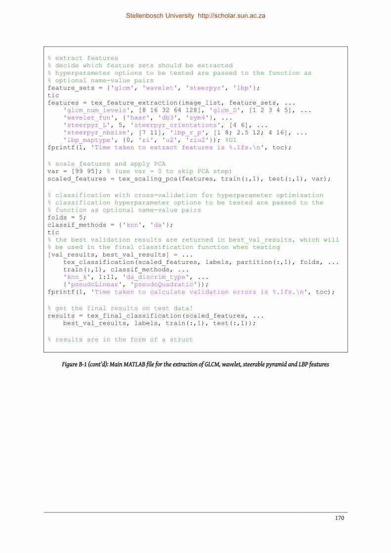
170
% extract features % decide which feature sets should be extracted % hyperparameter options to be tested are passed to the function as % optional name-value pairs feature_sets = {'glcm', 'wavelet', 'steerpyr', 'lbp'}; tic features = tex_feature_extraction(image_list, feature_sets, ... 'glcm_num_levels', [8 16 32 64 128], 'glcm_D', [1 2 3 4 5], ... 'wavelet_fun', {'haar', 'db3', 'sym4'}, ... 'steerpyr_L', 5, 'steerpyr_orientations', [4 6], ... 'steerpyr_nbsize', [7 11], 'lbp_r_p', [1 8; 2.5 12; 4 16], ... 'lbp_maptype', {0, 'ri', 'u2', 'riu2'}); %UI fprintf(1, 'Time taken to extract features is %.1fs.\n', toc);
% scale features and apply PCA var = [99 95]; % (use var = 0 to skip PCA step) scaled_features = tex_scaling_pca(features, train(:,1), test(:,1), var);
% classification with cross-validation for hyperparameter optimisation % classification hyperparameter options to be tested are passed to the % function as optional name-value pairs folds = 5; classif_methods = {'knn', 'da'}; tic % the best validation results are returned in best_val_results, which will % be used in the final classification function when testing [val_results, best_val_results] = ... tex_classification(scaled_features, labels, partition(:,1), folds, ... train(:,1), classif_methods, ... 'knn_k', 1:11, 'da_discrim_type', ... {'pseudoLinear', 'pseudoQuadratic'}); fprintf(1, 'Time taken to calculate validation errors is %.1fs.\n', toc);
% get the final results on test data! results = tex_final_classification(scaled_features, ... best_val_results, labels, train(:,1), test(:,1));
% results are in the form of a struct
Figure B-1 (cont’d): Main MATLAB file for the extraction of GLCM, wavelet, steerable pyramid and LBP features
Stellenbosch University http://scholar.sun.ac.za

171
% This is the main M-file that calls all functions in the texture analysis % toolbox in a logical order to read image data, extract features, classify % images and determine results.
% example is set up to analyse the coal data set % texton feature set is extracted
% format dataset % specify the folder in which the formatted data is to be stored tic new_folder = 'coal_data'; % specify a custimised function that converts the original image data to % the required format of equally sized RGB images format_function = @format_coal; % save the formatted data in the new folder and get the list of images image_list = tex_formatdata(format_function, new_folder); fprintf(1, 'Time taken to format data is %.1fs.\n', toc); % in this case the algorithm will say that the image data is already in the % correct format, since the correctly formatted data (and not the raw data) % was included with this toolbox
% define the labels for this data set using a custom function label_function = @label_coal; labels = tex_labeldata(label_function);
% partition the dataset into training and test data using the partitioning % method for the specific data set partition_function = @partition_coal; load_partition = false; save_partition = false; % train, test and partition are logical vectors indicating which images % belong to which sets [train, test, partition] = partition_function(load_partition, labels, ... save_partition);
% extract texton features tic % specify hyperparameters to be optimised texton_K = [20, 40, 80]; texton_fsize = [25, 49];
% Texton_frac_means is the fraction of the pixels that are used in the % clustering step. When performing the real analysis, this value was set to % 1, so all pixels were used. However, setting this fraction to a very low % number allows for the debugging of the texton algorithm without having to % wait days for it to execute. texton_frac_kmeans = 0.0000001; % fraction of pixels used in clustering % features are extracted features_texton = tex_texton_feature_extraction(image_list, train, ...
partition, texton_K, texton_fsize, texton_frac_kmeans); fprintf(1, 'Time taken to extract features is %.1fs.\n', toc);
Figure B-2: Main MATLAB file for the extraction of texton features
Stellenbosch University http://scholar.sun.ac.za

172
% scale features and apply PCA var = [95 99]; % (use var = 0 to skip PCA step) scaled_features_texton = tex_texton_scaling_pca(features_texton, ...
train(:,1), test(:,1), var);
% classification with cross-validation for hyperparameter optimisation % classification hyperparameter options to be tested are passed to the % function as optional name-value pairs folds = 5; classif_methods = {'knn', 'da'}; tic % the best validation results are returned in best_val_results, which will % be used in the final classification function when testing [val_results, best_val_results] = ... tex_texton_classification(scaled_features_texton, labels, ...
partition(:,1), folds, train(:,1), classif_methods, ... 'knn_k', 1:11, 'da_discrim_type', {'pseudoLinear', 'pseudoQuadratic'}); fprintf(1, 'Time taken to calculate validation errors is %.1fs.\n', toc);
% get the final results!
% extract features by using all training data % coal best_val_results: k40fsize25 (for both knn and da) partition_final = ones(size(partition)); % specify optimal hyperparameters as obtained during cross-validation step texton_K = 40; texton_fsize = 25; texton_frac_kmeans = 0.0000001; % again, set to 1 to obtain actual results tic features_texton_final = tex_texton_feature_extraction_final(image_list, ...
train, partition_final, ... texton_K, texton_fsize, texton_frac_kmeans); toc
% scale these final features var = [95 99]; scaled_features_texton_final = tex_scaling_pca(features_texton_final, ...
train, test, var);
% get the final results on the test data! results_texton = tex_final_classification(scaled_features_texton_final, ... best_val_results, labels, train, test);
% results are in the form of a struct
Figure B-2 (cont’d): Main MATLAB file for the extraction of texton features
Stellenbosch University http://scholar.sun.ac.za

173
Appendix C All repetition results: Coal on a conveyor belt
GLCM & K-NN
Repetition Test error
Avg. validation error
Std. validation error
Feature extraction hyperparameters K 𝐺 𝐷 PCA
1 30.0% 20.5% 5.5% 32 3 99% 11 2 24.3% 21.4% 2.9% 128 2 None 9 3 14.3% 24.8% 5.5% 8 5 None 9 4 31.4% 20.0% 3.6% 64 1 None 10 5 24.3% 24.3% 3.1% 8 5 99% 9 6 24.3% 20.0% 4.0% 8 2 None 4 7 28.6% 23.8% 6.7% 32 5 95% 6 8 21.4% 23.3% 5.9% 8 5 None 11 9 25.7% 21.0% 5.7% 16 2 None 8
10 31.4% 21.4% 2.9% 128 3 None 1 Avg. error 25.6% 22.0%
Std. error 5.2% 4.8%
Stellenbosch University http://scholar.sun.ac.za

174
GLCM & DA
Repetition Test error
Avg. validation error
Std. validation error
Feature extraction hyperparameters Type DA 𝐺 𝐷 PCA
1 22.9% 16.7% 4.8% 64 3 None Linear 2 8.6% 17.6% 8.0% 8 3 None Linear 3 18.6% 15.2% 4.9% 128 5 None Linear 4 22.9% 16.2% 3.5% 16 3 None Quadratic 5 15.7% 16.2% 4.6% 8 5 None Linear 6 12.9% 14.8% 4.6% 8 5 None Linear 7 18.6% 14.8% 3.5% 64 5 None Linear 8 18.6% 16.7% 2.4% 16 5 None Linear 9 18.6% 17.1% 1.1% 32 3 None Linear
10 12.9% 17.1% 9.7% 8 5 None Linear Avg. error 17.0% 16.2%
Std. error 4.5% 5.3%
Wavelet & K-NN
Repetition Test error
Avg. validation error
Std. validation error
Feature extraction hyperparameters K
Type wavelet PCA 1 12.9% 12.4% 6.4% ‘haar’ None 6 2 11.4% 16.2% 8.5% ‘haar’ None 9 3 11.4% 12.4% 3.9% ‘db3’ 95% 9 4 14.3% 13.3% 5.5% ‘haar’ None 10 5 15.7% 11.9% 5.3% ‘haar’ None 11 6 18.6% 11.9% 5.8% ‘db3’ 95% 3 7 17.1% 8.6% 4.0% ‘haar’ 99% 4 8 20.0% 13.8% 3.5% ‘haar’ 95% 6 9 17.1% 14.3% 7.3% ‘sym4’ 95% 3
10 8.6% 14.3% 5.3% ‘db3’ 99% 9 Avg. error 14.7% 12.9%
Std. error 3.6% 5.8%
Stellenbosch University http://scholar.sun.ac.za

175
Wavelet & DA
Repetition Test error
Avg. validation error
Std. validation error
Feature extraction hyperparameters Type DA
Type wavelet PCA 1 14.3% 11.4% 4.6% ‘haar’ 99% Linear 2 8.6% 15.2% 2.1% ‘haar’ None Linear 3 10.0% 12.4% 3.9% ‘haar’ None Linear 4 11.4% 15.7% 3.2% ‘haar’ None Linear 5 20.0% 11.9% 7.3% ‘haar’ None Linear 6 15.7% 12.4% 8.1% ‘haar’ 99% Quadratic 7 10.0% 12.4% 5.4% ‘haar’ 99% Linear 8 15.7% 10.5% 4.9% ‘haar’ None Linear 9 15.7% 12.4% 6.8% ‘haar’ 99% Linear
10 11.4% 13.8% 6.8% ‘haar’ 99% Linear Avg. error 13.3% 12.8%
Std. error 3.6% 5.6%
Steerable pyramid & K-NN
Repetition Test error
Avg. validation error
Std. validation error
Feature extraction hyperparameters K 𝑆𝑖𝑛𝑐 𝑊 PCA
1 18.6% 10.0% 5.2% 4 7 95% 4 2 15.7% 12.4% 3.9% 4 7 None 1 3 10.0% 12.9% 3.6% 4 7 None 7 4 12.9% 10.0% 5.2% 4 7 95% 6 5 11.4% 10.0% 5.4% 4 7 95% 6 6 11.4% 12.4% 2.6% 6 7 95% 10 7 21.4% 12.9% 4.9% 4 7 95% 10 8 11.4% 11.9% 3.4% 4 7 None 4 9 7.1% 11.9% 1.7% 4 7 95% 4
10 10.0% 12.9% 2.7% 6 7 None 4 Avg. error 13.0% 11.7% Std. error 4.3% 4.0%
Stellenbosch University http://scholar.sun.ac.za

176
Steerable pyramid & DA
Repetition Test error
Avg. validation error
Std. validation error
Feature extraction hyperparameters Type DA 𝑆𝑖𝑛𝑐 𝑊 PCA
1 7.1% 11.0% 3.2% 4 11 95% Linear 2 4.3% 10.5% 4.6% 6 7 95% Linear 3 7.1% 9.5% 1.7% 6 7 95% Linear 4 22.9% 9.5% 2.9% 6 7 None Linear 5 12.9% 7.6% 3.1% 6 7 95% Linear 6 21.4% 9.0% 4.3% 4 11 None Linear 7 14.3% 9.0% 5.4% 6 7 None Linear 8 11.4% 9.0% 2.6% 6 7 95% Linear 9 11.4% 8.1% 3.2% 6 7 95% Linear
10 7.1% 11.0% 6.0% 4 7 95% Linear Avg. error 12.0% 9.4% Std. error 6.2% 3.9%
Texton & K-NN
Repetition Test error
Avg. validation error
Std. validation error
Feature extraction hyperparameters K 𝐾𝑇 𝐹𝑆 PCA
1 8.6% 3.8% 2.1% 40 25 None 5
Texton & DA
Repetition Test error
Avg. validation error
Std. validation error
Feature extraction hyperparameters Type DA 𝐾𝑇 𝐹𝑆 PCA
1 10.0% 5.7% 2.7% 40 25 95% Quadratic
Stellenbosch University http://scholar.sun.ac.za

177
LBP & K-NN
Repetition Test error
Avg. validation error
Std. validation error
Feature extraction hyperparameters K
(𝑅, 𝑃) Mapping type PCA 1 8.6% 14.3% 5.3% (4, 16) ‘riu2’ 99% 8 2 18.6% 13.3% 4.0% (4, 16) ‘riu2’ None 11 3 10.0% 12.9% 6.4% (4, 16) ‘riu2’ 99% 6 4 14.3% 12.4% 4.9% (4, 16) ‘riu2’ None 6 5 15.7% 10.0% 3.1% (4, 16) ‘riu2’ 99% 5 6 20.0% 11.9% 5.1% (4, 16) ‘riu2’ 99% 3 7 21.4% 11.4% 4.3% (4, 16) ‘riu2’ 95% 3 8 21.4% 12.4% 4.3% (4, 16) ‘riu2’ 95% 4 9 10.0% 15.2% 6.4% (4, 16) ‘riu2’ None 10
10 11.4% 15.7% 3.2% (4, 16) ‘riu2’ None 8 Avg. error 15.1% 13.0% Std. error 5.0% 4.8%
LBP & DA
Repetition Test error
Avg. validation error
Std. validation error
Feature extraction hyperparameters Type DA
(𝑅, 𝑃) Mapping type PCA 1 7.1% 9.0% 4.3% (2.5, 12) ‘riu2’ None Linear 2 10.0% 8.1% 4.9% (2.5, 12) ‘riu2’ 99% Linear 3 12.9% 9.0% 2.6% (4, 16) ‘riu2’ None Linear 4 11.4% 7.1% 3.8% (2.5, 12) ‘riu2’ None Linear 5 10.0% 6.7% 3.5% (2.5, 12) ‘riu2’ 99% Linear 6 12.9% 8.1% 2.1% (4, 16) ‘riu2’ 99% Linear 7 14.3% 9.0% 3.9% (2.5, 12) ‘riu2’ 99% Linear 8 12.9% 8.6% 2.7% (2.5, 12) ‘riu2’ 99% Linear 9 7.1% 8.1% 5.2% (2.5, 12) ‘riu2’ None Linear
10 4.3% 8.6% 2.1% (4, 16) ‘riu2’ 99% Linear Avg. error 10.3% 8.2% Std. error 3.2% 3.7%
Stellenbosch University http://scholar.sun.ac.za

178
Appendix D All repetition results: Hydrocyclone underflows
GLCM & K-NN
Repetition Test error
Avg. validation error
Std. validation error
Feature extraction hyperparameters K 𝐺 𝐷 PCA
1 13.5% 12.0% 2.0% 32 5 None 4 2 12.2% 15.0% 1.8% 128 5 99% 3 3 18.9% 11.1% 5.0% 32 5 None 4 4 10.8% 15.9% 1.0% 64 5 None 8 5 20.3% 10.2% 2.4% 32 5 None 4 6 18.9% 12.9% 9.0% 8 5 99% 1 7 10.8% 14.6% 4.6% 64 5 None 5 8 14.9% 14.6% 3.6% 16 5 None 5 9 9.5% 13.3% 6.5% 128 5 99% 4
10 12.2% 12.4% 6.7% 64 5 None 4 Avg. error 14.2% 13.2%
Std. error 3.9% 4.9%
Stellenbosch University http://scholar.sun.ac.za

179
GLCM & DA
Repetition Test error
Avg. validation error
Std. validation error
Feature extraction hyperparameters Type DA 𝐺 𝐷 PCA
1 13.5% 8.9% 4.2% 64 5 None Quadratic 2 13.5% 11.5% 1.8% 16 5 99% Quadratic 3 14.9% 8.4% 3.3% 64 4 99% Linear 4 9.5% 13.3% 4.6% 64 5 None Linear 5 16.2% 9.7% 3.0% 8 5 None Quadratic 6 17.6% 8.9% 6.3% 32 5 None Quadratic 7 10.8% 11.1% 7.9% 16 5 None Quadratic 8 14.9% 11.1% 4.4% 128 5 None Linear 9 16.2% 11.0% 4.3% 8 3 99% Quadratic
10 8.1% 11.0% 4.6% 32 5 None Quadratic Avg. error 13.5% 10.5%
Std. error 3.1% 4.7%
Wavelet & K-NN
Repetition Test error
Avg. validation error
Std. validation error
Feature extraction hyperparameters K
Type wavelet PCA 1 12.2% 11.1% 4.5% ‘db3’ None 1 2 9.5% 12.4% 4.4% ‘db3’ 99% 4 3 13.5% 13.3% 3.4% ‘db3’ 99% 3 4 12.2% 11.5% 2.8% ‘db3’ 99% 4 5 13.5% 11.1% 5.4% ‘db3’ None 4 6 18.9% 11.1% 4.5% ‘db3’ None 7 7 12.2% 13.7% 4.9% ‘db3’ None 4 8 10.8% 9.3% 3.2% ‘db3’ 99% 4 9 13.5% 11.9% 6.7% ‘db3’ None 1
10 13.5% 11.5% 2.9% ‘db3’ None 1 Avg. error 13.0% 11.7%
Std. error 2.5% 4.4%
Stellenbosch University http://scholar.sun.ac.za

180
Wavelet & DA
Repetition Test error
Avg. validation error
Std. validation error
Feature extraction hyperparameters Type DA
Type wavelet PCA 1 6.8% 11.1% 4.5% ‘sym4’ None Linear 2 5.4% 11.5% 1.8% ‘sym4’ None Linear 3 18.9% 10.6% 4.7% ‘haar’ None Linear 4 12.2% 10.2% 2.5% ‘sym4’ None Linear 5 10.8% 10.6% 3.3% ‘sym4’ None Linear 6 14.9% 10.2% 5.8% ‘sym4’ None Linear 7 18.9% 12.4% 8.0% ‘haar’ None Linear 8 12.2% 11.0% 4.4% ‘sym4’ None Linear 9 9.5% 10.6% 3.5% ‘sym4’ None Linear
10 13.5% 11.1% 6.1% ‘sym4’ None Linear Avg. error 12.3% 10.9%
Std. error 4.5% 4.8%
Steerable pyramid & K-NN
Repetition Test error
Avg. validation error
Std. validation error
Feature extraction hyperparameters K 𝑆𝑖𝑛𝑐 𝑊 PCA
1 14.9% 7.9% 6.1% 6 11 95% 1 2 9.5% 8.4% 4.3% 4 11 None 1 3 16.2% 8.8% 3.4% 4 11 None 1 4 5.4% 7.5% 4.5% 6 11 None 1 5 14.9% 8.8% 3.4% 6 11 95% 3 6 12.2% 9.3% 6.6% 6 11 99% 1 7 6.8% 8.8% 4.1% 6 11 None 1 8 5.4% 8.0% 5.3% 4 11 99% 1 9 10.8% 8.8% 6.1% 6 11 95% 4
10 10.8% 8.4% 2.9% 6 11 None 1 Avg. error 10.7% 8.5% Std. error 4.0% 4.8%
Stellenbosch University http://scholar.sun.ac.za
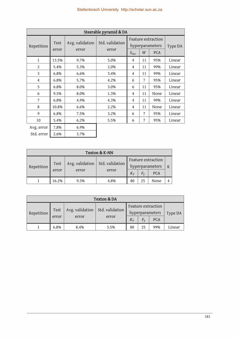
181
Steerable pyramid & DA
Repetition Test error
Avg. validation error
Std. validation error
Feature extraction hyperparameters Type DA 𝑆𝑖𝑛𝑐 𝑊 PCA
1 13.5% 9.7% 5.0% 4 11 95% Linear 2 5.4% 5.3% 2.0% 4 11 99% Linear 3 6.8% 6.6% 3.4% 4 11 99% Linear 4 6.8% 5.7% 4.2% 6 7 95% Linear 5 6.8% 8.0% 3.0% 6 11 95% Linear 6 9.5% 8.0% 1.3% 4 11 None Linear 7 6.8% 4.9% 4.3% 4 11 99% Linear 8 10.8% 6.6% 2.2% 4 11 None Linear 9 6.8% 7.5% 3.2% 6 7 95% Linear
10 5.4% 6.2% 5.5% 6 7 95% Linear Avg. error 7.8% 6.9% Std. error 2.6% 3.7%
Texton & K-NN
Repetition Test error
Avg. validation error
Std. validation error
Feature extraction hyperparameters K 𝐾𝑇 𝐹𝑆 PCA
1 16.2% 9.3% 4.8% 80 25 None 4
Texton & DA
Repetition Test error
Avg. validation error
Std. validation error
Feature extraction hyperparameters Type DA 𝐾𝑇 𝐹𝑆 PCA
1 6.8% 8.4% 3.5% 80 25 99% Linear
Stellenbosch University http://scholar.sun.ac.za

182
LBP & K-NN
Repetition Test error
Avg. validation error
Std. validation error
Feature extraction hyperparameters K
(𝑅, 𝑃) Mapping type PCA 1 13.5% 11.1% 5.4% (4, 16) ‘u2’ None 6 2 12.2% 12.4% 6.9% (4, 16) ‘u2’ 99% 5 3 8.1% 9.7% 2.9% (4, 16) ‘u2’ None 4 4 8.1% 11.0% 4.8% (4, 16) ‘u2’ None 4 5 8.1% 12.0% 4.6% (4, 16) ‘u2’ None 8 6 10.8% 10.2% 6.0% (4, 16) ‘u2’ None 10 7 14.9% 8.4% 3.3% (4, 16) ‘u2’ 99% 6 8 9.5% 12.0% 5.6% (4, 16) ‘u2’ None 9 9 10.8% 11.1% 1.6% (4, 16) ‘u2’ 99% 4
10 8.1% 12.0% 4.4% (4, 16) ‘u2’ None 4 Avg. error 10.4% 11.0% Std. error 2.5% 4.8%
LBP & DA
Repetition Test error
Avg. validation error
Std. validation error
Feature extraction hyperparameters Type DA
(𝑅, 𝑃) Mapping type PCA 1 9.5% 8.9% 3.1% (1, 8) ‘u2’ 99% Linear 2 10.8% 7.1% 1.8% (1, 8) ‘u2’ None Linear 3 13.5% 7.5% 3.3% (1, 8) ‘u2’ None Linear 4 9.5% 8.8% 2.6% (4, 16) ‘u2’ 99% Linear 5 8.1% 8.0% 4.6% (4, 16) ‘riu2’ None Linear 6 6.8% 8.0% 4.3% (1, 8) ‘u2’ 99% Linear 7 9.5% 7.1% 2.4% (4, 16) ‘riu2’ None Linear 8 4.1% 9.7% 5.6% (4, 16) ‘riu2’ None Linear 9 12.2% 8.4% 1.8% (1, 8) ‘u2’ 99% Linear
10 9.5% 9.3% 3.6% (1, 8) ‘u2’ 99% Linear Avg. error 10.3% 8.2% Std. error 3.2% 3.7%
Stellenbosch University http://scholar.sun.ac.za

183
Appendix E Publications based on this work
E-1 International peer-reviewed journal paper Kistner, M., Jemwa, G. & Aldrich, C., 2013. Monitoring of mineral processing systems by using textural image analysis. Minerals Engineering, 52, p. 169–177.
E-2 Peer-reviewed conference proceedings paper Aldrich, C., Jemwa, G. & Munnik, M., 2012. Image textural features and semi-supervised learning: An application to classification of coal particles. 3rd International Congress on Automation in the Mining Industry, Automining 2012. Chile, Gecamin.
E-3 Non-peer-reviewed presentation at conference Kistner, M., Auret, L. & Aldrich, C., 2013. A structured image texture analysis approach to inferential sensing in mineral processes. [Mineral Processing 2013, Cape Town, South Africa, 7–8 August 2013]
Stellenbosch University http://scholar.sun.ac.za

184
“Learn from yesterday, live for today, hope for tomorrow. The important thing is to not stop questioning.” – Albert Einstein
Stellenbosch University http://scholar.sun.ac.za