Image Segmentation using Normalized Graph Cut

By W A T Mahesh Dananjaya

110089M

Abstract: Image Processing is becoming paramount important technology to the modern world since it

is the caliber behind the machine learning and so called artificial intelligence. Image segmentation is

one of the major area of the modern image processing and computer vision. Many computer vision

researches that have been carrying out emerge the important of pattern analysis and perceptual vision of

a scene and regression of features. Image segmentation is inherent strength of image processing

techniques for pattern recognition and regression.

Normalized Graph cut method was proposed by Jianbo Shi and Jitendra Malik to address the

problem of perceptual grouping and organization in vision. Proposed method has provided a powerful

way of extracting and understanding of the global impression of the image rather than focusing heavily

on the local features and their consistencies in the image data. In this approach image is considered as

a Graph of image nodes and apply the solution in the way of graph partitioning problem. This method

was really address the drawbacks of exist image segmentation method using minimum cut. This

methodology has provided the new measure of graph partitioning called disassociation measure the

normalized cuts by taking total edge connection to all the nodes in the graph to compute the cut cost.

Normalized cut method is not only taking total dissimilarity between the different groups, but also it

takes total similarities within a group for the graph partitioning process. This method has come up with

advanced algorithm comprising with solution of generalized eigenvalue problem for optimal graph

partitioning including prevailing knowledge on image clustering grouping and segmentation.

1. Introduction

1.1 Minimum Cut

Although there were boundary based and region based methodologies for image clustering those

techniques do not provide a global impression for the computer vision based applications. Graph

partitioning is the most available and sustainable way to absorb global perception of an image rather

than focusing on local properties of the image. Therefore Graph theories and Eigen vector based methods

are used to achieve an optimal solution to image segmentation previously. Wu and Leahy proposed an

image clustering methodology based on minimum cut criteria compromising the optimal graph

portioning. In their method, they partition a graph into k-sub graphs in a way that the maximum cut

across the sub graph is minimized. This globally optimal criterion can be used to produce good

segmentation on some of the images. But this minimum cut is not always favorable. This criteria favors

cutting small sets of isolated nodes in the graph and gives bad partitioning when cost (weight) function

is inverse to the distance (Similarity) between nodes.

In the graph partitioning approach first the given image is taken as graph G= (V, E) and then segmented.

The Minimum cut method sometimes gives bad partitioning because this method is only looking at the

value of total edge weight connecting the two partition and no measure or parameter is used to indicate

the number of edge connection as a fraction of total connection to all the nodes in the graph.

In usual graph partitioning graph G= (V, E) is partitioned into two disjoint sub sets, A, B such that

A𝐴 ∪ 𝐵 ≡ 𝑉 𝑎𝑛𝑑 𝐴 ∩ 𝐵 ≡ ∅ by simply removing edges connecting the two parts. The degree of

dissimilarity between these two pieces can be computed as total weight of the edges that have been

removed. Cut is defined as:

𝐶𝑢𝑡 (𝐴, 𝐵) = 𝑤(𝑢, 𝑣)𝑢∈𝐴,𝑣∈𝐵 (1)

In minimum cut criteria the optimal partitioning of the graph is the cut that minimizes the total cost or

weight of the cut as the cost is inversely proportional to the distance or similarity between nodes. This

emerges the inherent drawback of the minimum cut criteria. Therefore the problem remains with the

isolated point in an image segmentation and clustering when we use minimum cuts. Requirement for the

novel method with a new measure of association of graph node is accomplished by the normalized cut

technique.

1.2 Normalized Cut

In this new method new measure to defined to calculate the association between nodes for a

graph cut. This usually known as disassociation measure the normalized cut.

𝑁𝑐𝑢𝑡 (𝐴, 𝐵) =𝑐𝑢𝑡(𝐴,𝐵)

𝑎𝑠𝑠𝑜𝑐(𝐴,𝑉)+

𝑐𝑢𝑡(𝐴,𝐵)

𝑎𝑠𝑠𝑜𝑐(𝐵,) (2)

Where 𝑎𝑠𝑠𝑜𝑐(𝐴, 𝑉) = 𝑤(𝑢, 𝑡)𝑢∈𝐴,𝑡∈𝑉 is the total connection from node in A to all nodes in the graph

and 𝑎𝑠𝑠𝑜𝑐(𝐵, 𝑉) = 𝑤(𝑣, 𝑡)𝑣∈𝐵,𝑡∈𝑉 is the total connection from node in B to all nodes in the graph.

In this new way of defining disassociation between groups, the isolated points are no longer appear and

no longer have small Ncut values. Because of the assoc value is much smaller and provide large Ncut

value. And also we can define a measure for total normalized association within group for a given

partition.

𝑁𝑎𝑠𝑠𝑜𝑐(𝐴, 𝐵) =𝑎𝑠𝑠𝑜𝑐(𝐴,𝐴)

𝑎𝑠𝑠𝑜𝑐(𝐴,𝑉)+

𝑎𝑠𝑠𝑜𝑐(𝐵,𝐵)

𝑎𝑠𝑠𝑜𝑐(𝐵,𝑉) (3)

And also we can derived an important property between Ncut and Nassoc.

𝑁𝑐𝑢𝑡(𝐴, 𝐵) = 2 − 𝑁𝑎𝑠𝑠𝑜𝑐(𝐴, 𝐵) (4)

Therefore this graph partitioning algorithm minimize the disassociation

between the groups and maximize the association within the groups. Therefore it is essential to

have a normalized cut as the partitioning criteria.

2. Methodology

2.1 Optimal Partition and Generalized Eigenvalue Problem

Let 𝑑(𝑖) = 𝜔(𝑖, 𝑗)𝑗 be the total number of connection from node I to all other nodes. D

be the N× 𝑁 diagonal matrix with 𝑑(𝑖) on its diagonal.

Let W be a 𝑁 × 𝑁 symmetric matrix with𝑊(𝑖, 𝑗) = 𝑤(𝑖, 𝑗).

By complex mathematical calculation we can show that this optimal partitioning problem

is converged to the following expression.

𝑚𝑖𝑛𝐴,𝐵𝑁𝑐𝑢𝑡(𝐴, 𝐵) = 𝑚𝑖𝑛𝑦𝑦𝑇(𝐷−𝑊)𝑦

𝑦𝑇𝐷𝑦 (5)

And if y is relaxed y is relaxed to take real value, we can minimize (5) by solving generalized

eigenvalue problem.

(𝐷 − 𝑊)𝑦 = 𝛾𝐷𝑦 (6)

2.2 Design steps

Step 1: Given an image sequence I and N=number of pixels

I – Image Sequence

Step 2: Construct the Weighted Graph G= (V, E) where each node represent a pixel in the

image I. N= |V| = number of nodes (pixels) in the graph

𝐺 = (𝑉, 𝐸)

N= |V|

Step 3: W-Compute the N N weighted matrix (Similarity) as

𝑒𝑥𝑝− 𝑋(𝑖)−𝑋(𝑗)

2

2

𝜎𝑋2

𝑖𝑓 𝑋(𝑖) − 𝑋(𝑗) 2< 𝑟

𝑤(𝑖, 𝑗) = 𝑒𝑥𝑝− 𝐹(𝑖)−𝐹(𝑗)

2

2

𝜎𝐼2 × 0 else

Where 𝑋 ( 𝑖 ) is the spatial location of node I, i.e. the coordinate in the original image I

𝑎𝑛𝑑 𝐹(𝑖) is a feature vector defined as:

𝐹(𝑖) = 1 for segmentation point set

𝐹(𝑖) = 𝐼(𝑖) the intensity value for segmentation brightness (gray scale) images

𝐹(𝑖) = [𝑣, 𝑣. 𝑠. 𝑠𝑖𝑛(ℎ), 𝑣. 𝑠. 𝑐𝑜𝑠(ℎ)](𝑖) Where h, s, v are the HSV values for

color segmentation

𝐹(𝑖) = [ 𝐼 ∗ 𝑓1 , … , 𝐼 ∗ 𝑓𝑛 ](𝑖) 𝑤ℎ𝑒𝑟𝑒 𝑡ℎ𝑒 𝑓𝑖 are DOOG filter at various scale

and orientation

Let 𝑑(𝑖) = 𝑤(𝑖, 𝑗)𝑗 be the total connection from node I to all other node.

Step 4: D-Construct an N*N diagonal matrix D with d on its diagonal

Step 5: Model and Solve generalized Eigenvalue System

(𝐷 − 𝑊)𝑦 = 𝛾𝐷𝑦

Solve and get the eigenvector with the second smallest eigenvalue.

Step 6: Bi-Partitioning the graph

By using the eigenvector to bipartition the graph. In ideal case eigenvector only take on

two discrete values and the signs tell us how to partition the graph

( 𝐴 = 𝑉𝑖 𝑌𝑖 > 0 ), 𝐵 = 𝑉𝑖 𝑌𝑖 ≤ 0

However y is relaxed to take real value other than discrete values. So it is essential to select

splitting point. We can use various methods choose splitting point.

0 value

Median value

Search a splitting point which result in that 𝑁𝑐𝑢𝑡 (𝐴, 𝐵) is minimized.

That will satisfy the equation that we derived earlier

𝑚𝑖𝑛𝐴,𝐵𝑁𝑐𝑢𝑡(𝐴, 𝐵) = 𝑚𝑖𝑛𝑦𝑦𝑇(𝐷−𝑊)𝑦

𝑦𝑇𝐷𝑦 By minimizing

𝑦𝑇(𝐷−𝑊)𝑦

𝑦𝑇𝐷𝑦

For (5) and (6) we have to some mathematical calculations which are not going to be

covered in this paper. There we put a substitution.

𝑌 = (1 + 𝑥) − 𝑏(1 − 𝑥) Where 𝑏 = 𝑘/(1 − 𝑘)

𝑘 = 𝑑𝑖𝑥𝑖>0

𝑑𝑖𝑖

To find the minimum Ncut, we need to try different values of splitting points. The

optimal splitting point is generally around the mean value of the obtained eigenvector.

Step 7: Recursive Repartition

Repeat bipartition process recursively until some constraint will be acquired by the

program. We can stop if Ncut value is larger than a pre specified threshold value. There

is another constraint. We can stop if the partition area is smaller than a pre specified

threshold value. Those are little advancement for the original program.

3. ADVANCEMENTS & DEVELOPMENTS

Apart from the original concept of the research carried out by Shi I have added some

more features in to the algorithm based on the previous development of the same

concept. I have inserted another two parameters to restrict the unwanted processing

power.

SNV -> Smallest Normalized-Cut Value

SNA -> Smallest Normalized-Cut Area

SNV is used to stop the process if the Ncut value of the partition is smaller than pre

specified SNV (threshold) value.

SNA is used to stop the process if the total number of nodes in the partition (Area)is

smaller than the pre specified threshold (SNA)value.

These two Threshold values terminate the unwanted recursive bipartition of out

grouping algorithm.

4. Experimental Results

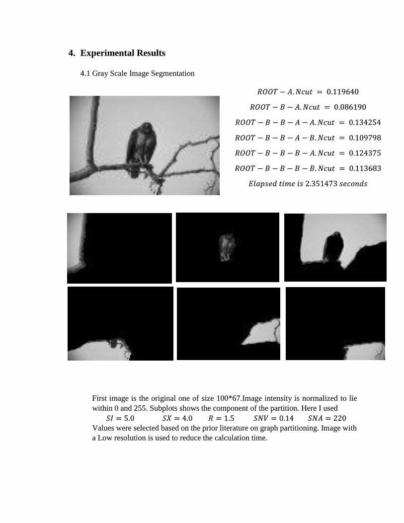
4.1 Gray Scale Image Segmentation

First image is the original one of size 100*67.Image intensity is normalized to lie

within 0 and 255. Subplots shows the component of the partition. Here I used

𝑆𝐼 = 5.0 𝑆𝑋 = 4.0 𝑅 = 1.5 𝑆𝑁𝑉 = 0.14 𝑆𝑁𝐴 = 220

Values were selected based on the prior literature on graph partitioning. Image with

a Low resolution is used to reduce the calculation time.

𝑅𝑂𝑂𝑇 − 𝐴.𝑁𝑐𝑢𝑡 = 0.119640

𝑅𝑂𝑂𝑇 − 𝐵 − 𝐴.𝑁𝑐𝑢𝑡 = 0.086190

𝑅𝑂𝑂𝑇 − 𝐵 − 𝐵 − 𝐴 − 𝐴.𝑁𝑐𝑢𝑡 = 0.134254

𝑅𝑂𝑂𝑇 − 𝐵 − 𝐵 − 𝐴 − 𝐵.𝑁𝑐𝑢𝑡 = 0.109798

𝑅𝑂𝑂𝑇 − 𝐵 − 𝐵 − 𝐵 − 𝐴.𝑁𝑐𝑢𝑡 = 0.124375

𝑅𝑂𝑂𝑇 − 𝐵 − 𝐵 − 𝐵 − 𝐵.𝑁𝑐𝑢𝑡 = 0.113683

𝐸𝑙𝑎𝑝𝑠𝑒𝑑 𝑡𝑖𝑚𝑒 𝑖𝑠 2.351473 𝑠𝑒𝑐𝑜𝑛𝑑𝑠

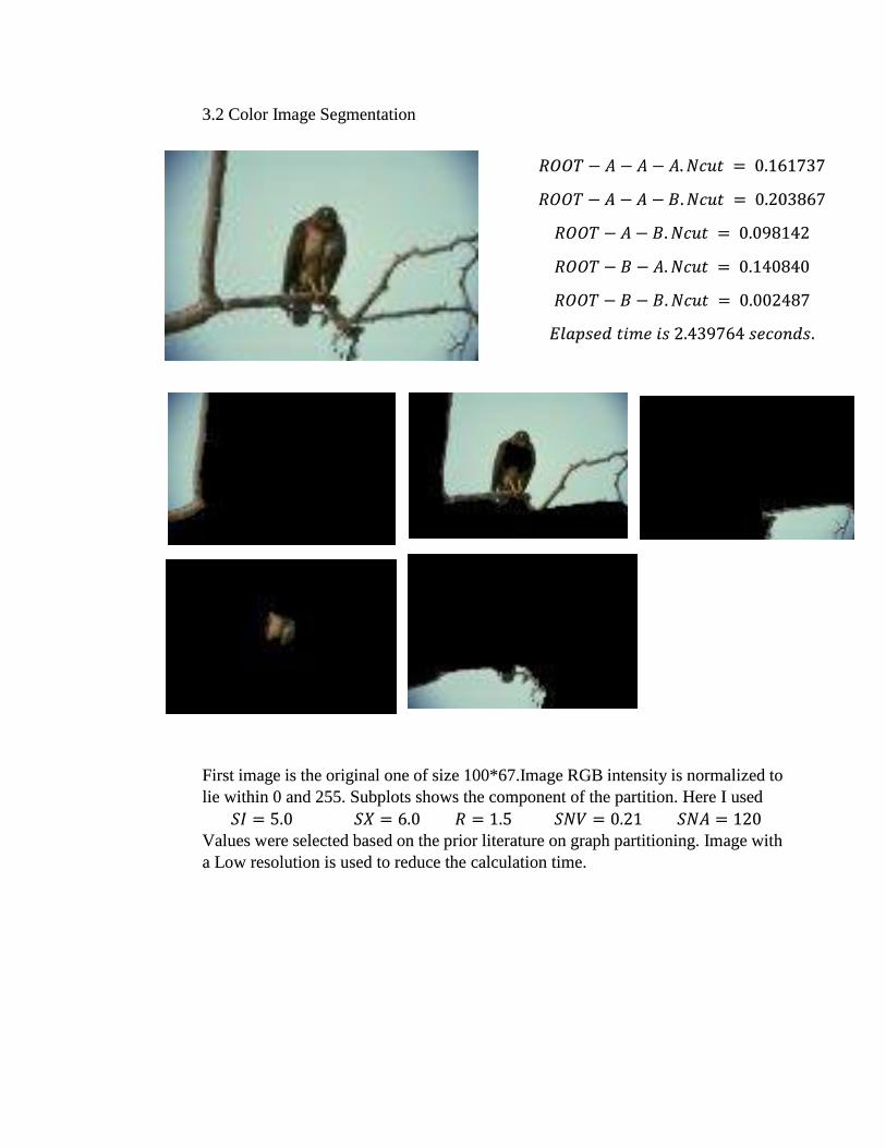
3.2 Color Image Segmentation

First image is the original one of size 100*67.Image RGB intensity is normalized to

lie within 0 and 255. Subplots shows the component of the partition. Here I used

𝑆𝐼 = 5.0 𝑆𝑋 = 6.0 𝑅 = 1.5 𝑆𝑁𝑉 = 0.21 𝑆𝑁𝐴 = 120

Values were selected based on the prior literature on graph partitioning. Image with

a Low resolution is used to reduce the calculation time.

𝑅𝑂𝑂𝑇 − 𝐴 − 𝐴 − 𝐴.𝑁𝑐𝑢𝑡 = 0.161737

𝑅𝑂𝑂𝑇 − 𝐴 − 𝐴 − 𝐵.𝑁𝑐𝑢𝑡 = 0.203867

𝑅𝑂𝑂𝑇 − 𝐴 − 𝐵.𝑁𝑐𝑢𝑡 = 0.098142

𝑅𝑂𝑂𝑇 − 𝐵 − 𝐴.𝑁𝑐𝑢𝑡 = 0.140840

𝑅𝑂𝑂𝑇 − 𝐵 − 𝐵.𝑁𝑐𝑢𝑡 = 0.002487

𝐸𝑙𝑎𝑝𝑠𝑒𝑑 𝑡𝑖𝑚𝑒 𝑖𝑠 2.439764 𝑠𝑒𝑐𝑜𝑛𝑑𝑠.

5. Comparison The results are compared with the original implementation of Dr.Shi. According to

Resuts it took nearly minutes for the calculation for the Dr.Shi.

But My program is work much better and took only 10 seconds to complete the

work.

𝑅𝑂𝑂𝑇 − 𝐴 − 𝐴.𝑁𝑐𝑢𝑡 = 0.119519

𝑅𝑂𝑂𝑇 − 𝐴 − 𝐵 − 𝐴.𝑁𝑐𝑢𝑡 = 0.027895

𝑅𝑂𝑂𝑇 − 𝐴 − 𝐵 − 𝐵.𝑁𝑐𝑢𝑡 = 0.000000

𝑅𝑂𝑂𝑇 − 𝐵 − 𝐴.𝑁𝑐𝑢𝑡 = 0.026061

𝑅𝑂𝑂𝑇 − 𝐵 − 𝐵.𝑁𝑐𝑢𝑡 = 0.020161

𝐸𝑙𝑎𝑝𝑠𝑒𝑑 𝑡𝑖𝑚𝑒 𝑖𝑠 10.907697 𝑠𝑒𝑐𝑜𝑛𝑑𝑠.

6. REFERENCES

[1] Jianbo Shi and Jitendra Malik, "Normalized Cuts and Image

Segmentation," IEEE Transactions on PAMI, Vol. 22, No. 8, Aug. 2000.

http://www.cs.berkeley.edu/~malik/papers/SM-ncut.pdf

[2] Graph Based Image Segmentation Tutorial

http://www.cis.upenn.edu/~jshi/GraphTutorial/

[3] MATLAB Normalized Cuts Segmentation Code

http://www.cis.upenn.edu/~jshi/software/

[4] D. Martin and C. Fowlkes and D. Tal and J. Malik, "A Database of

Human Segmented Natural Images and its Application to Evaluating

Segmentation Algorithms and Measuring Ecological Statistics",

Proc. 8th Int'l Conf. Computer Vision, vol. 2, pp. 416-423, July 2001.

http://www.eecs.berkeley.edu/Research/Projects/CS/vision/bsds/

7. APPENDIX

calcNcutSegment.m

function Iseg = calcNcutSegment(I, SI, SX, R, SNV, SNA) % NcutImageSegment - Normalized Cuts and Image Segmentation [1] % [SegI] = NcutImageSegment(I, SI, SX, r, SNV, SNA) % Parameters % I NR*NC*C Image Matrix % SI Coefficient Related to Feature % SX Coefficient related to Position % R Coefficient used to compute similarity (weight) matrix % SNV Smalllest Normalized-Cut Value(Threashold) % SNA Smallest Normalized-Cut Area (Threshols) % SegI cell array of segmented images of NR*NC*C [NR, NC, C] = size(I); % Step 1 : Calculate |V|=N N = NR * NC; % Step 2: Construcyt Nodes (Vertices) of the Grapg G=(V,E) V = reshape(I, N, C); % Step 3. Compute weight matrix W and D W = calcNcutW(I, SI, SX, R); % Step 7. recursively repartition Seg = (1:N)'; % the first segment has whole nodes. [1 2 3 ... N]' [Seg Id Ncut] = calcNcutPartition(Seg, W, SNV, SNA, 'ROOT'); % Convert node ids into images for i=1:length(Seg) subV = zeros(N, C); %ones(N, c) * 255; subV(Seg{i}, :) = V(Seg{i}, :); Iseg{i} = uint8(reshape(subV, NR, NC, C)); fprintf('%s. Ncut = %f\n', Id{i}, Ncut{i}); end

end

calcNcutW.m

function W = calcNcutW(I, SI, SX, R); % NcutComputeW - Compute a similarity (weight) matrix [NR, NC, C] = size(I); N = NR* NC; W = sparse(N,N); % Feature Vectors if C == 3 F = F3(I); else F = F2(I); end F = reshape(F, N, 1, C); X = cat(3, repmat((1:NR)', 1, NC), repmat((1:NC), NR, 1)); X = reshape(X, N, 1, 2);

for ic=1:NC for ir=1:NR

% This range satisfies |X(i) - X(j)| <= r (block distance) jc = (ic - floor(R)) : (ic + floor(R)); % vector jr = ((ir - floor(R)) :(ir + floor(R)))'; jc = jc(jc >= 1 & jc <= NC); jr = jr(jr >= 1 & jr <= NR); jN = length(jc) * length(jr);

% index at vertex. V(i) i = ir + (ic - 1) * NR; j = repmat(jr, 1, length(jc)) + repmat((jc -1) * NR, length(jr),

1); j = reshape(j, length(jc) * length(jr), 1); % a col vector

% spatial location distance (disimilarity) XJ = X(j, 1, :); XI = repmat(X(i, 1, :), length(j), 1); DX = XI - XJ; DX = sum(DX .* DX, 3); % squared euclid distance %DX = sum(abs(DX), 3); % block distance % square (block) reagion may work better for skew lines than circle

(euclid) reagion.

% |X(i) - X(j)| <= r (already satisfied if block distance

measurement) constraint = find(sqrt(DX) <= R); j = j(constraint); DX = DX(constraint);

% feature vector disimilarity FJ = F(j, 1, :); FI = repmat(F(i, 1, :), length(j), 1);

DF = FI - FJ; DF = sum(DF .* DF, 3); % squared euclid distance %DF = sum(abs(DF), 3); % block distance

% Hint: W(i, j) is a col vector even if j is a matrix W(i, j) = exp(-DF / (SI*SI)) .* exp(-DX / (SX*SX)); % for squared

distance %W(i, j) = exp(-DF / SI) .* exp(-DX / SX); end end end

% F1 - F4: Compute a feature vector F % F = F1(I) % for point sets % F = F2(I) % intensity % F = F3(I) % hsv, for color % F = F4(I) % DOOG %

function F = F1(I); F = (I == 0); end function F = F2(I); % intensity, for gray scale F = I; end function F = F3(I); F = I; % raw RGB end function F = F4(I); % DOOG, for texture % Future End

calcNcutPartition.m

function [Seg Id Ncut] = calcNcutPartition(I, W,SNV,SNA, ID)

% Compute D N = length(W); d = sum(W, 2); D = spdiags(d, 0, N, N); % diagonal matrix

% Step 2 and 3. Solve generalized eigensystem (D -W)*S = S*D*U (12).

warning off; % let me stop warning [U,S] = eigs(D-W, D, 2, 'sm'); % 2nd smallest (1st smallest has all same value elements, and useless) U2 = U(:, 2); % T = abs(U2); m = max(T); T = T / m * 255; imshow(uint8(reshape(T, 15,

20))); % Step 3. Refer 3.1 Example 3. % (1). Bipartition the graph at 0 (hopefully, eigenvector can be % splitted by + and -). % This did not work well. %A = find(U2 > 0);

%B = find(U2 <= 0); % (2). Bipartition the graph at median value. %t = median(U2); %A = find(U2 > t); %B = find(U2 <= t); % (3). Bipartition the graph at point that Ncut is minimized. t = mean(U2); t = fminsearch('NcutValue', t, [], U2, W, D); A = find(U2 > t); B = find(U2 <= t);

% Step 4. Decide if the current partition should be divided % if either of partition is too small, stop recursion. % if Ncut is larger than threshold, stop recursion. ncut = calcNcutValue(t, U2, W, D); if (length(A) < SNA || length(B) < SNA) || ncut > SNV Seg{1} = I; Id{1} = ID; % for debugging Ncut{1} = ncut; % for duebuggin return; end

% Seg segments of A [SegA IdA NcutA] = NcutPartition(I(A), W(A, A), SNV, SNA, [ID '-A']); % I(A): node index at V. A is index at the segment, I % W(A, A); % weight matrix in segment A

% Seg segments of B [SegB IdB NcutB] = NcutPartition(I(B), W(B, B), SNV, SNA, [ID '-B']); % concatenate cell arrays Seg = [SegA SegB]; Id = [IdA IdB]; Ncut = [NcutA NcutB]; end

calcNcutValue.m

function ncut = calcNcutValue(t, U2, W, D); % NcutValue - Computing the Optimal Partition Ncut x = (U2 > t); x = (2 * x) - 1; d = diag(D); k = sum(d(x > 0)) / sum(d); b = k / (1 - k); y = (1 + x) - b * (1 - x); ncut = (y' * (D - W) * y) / ( y' * D * y ); end