Image Processing Toolbox -...

Computation

Visualization

Programming

For Use with MATLAB®

Image ProcessingToolbox

User’s GuideVersion 3

1

Getting Started

This section contains two examples to get you started doing image processing using MATLAB and the Image Processing Toolbox. The examples contain cross-references to other sections in this manual that have in-depth discussions on the concepts presented in the examples.

Example 1 — Some Basic Topics (p. 1-2)

Guides you through an example of some of the basic image processing capabilities of the toolbox, including reading, writing, and displaying images

Example 2 — Advanced Topics (p. 1-9) Guides you through some more advanced image processing topics including components labeling, object property measurement, image arithmetic, morphological image processing, and contrast enhancement

Where to Go from Here (p. 1-23) Provides pointers to additional sources of information

1 Getting Started

1-2

Example 1 — Some Basic TopicsBefore beginning with this exercise, start MATLAB. If you are new to MATLAB, you should first read the MATLAB Getting Started documentation.

You should already have installed the Image Processing Toolbox, which runs seamlessly from MATLAB. For information about installing the toolbox, see the MATLAB Installation Guide for your platform.

All of the images used in this example are supplied with the Image Processing Toolbox. Note that the images shown in this documentation differ slightly from what you see on your screen because the surrounding MATLAB figure window has been removed to save space.

1. Read and Display an ImageClear the MATLAB workspace of any variables and close open figure windows.

clear, close all

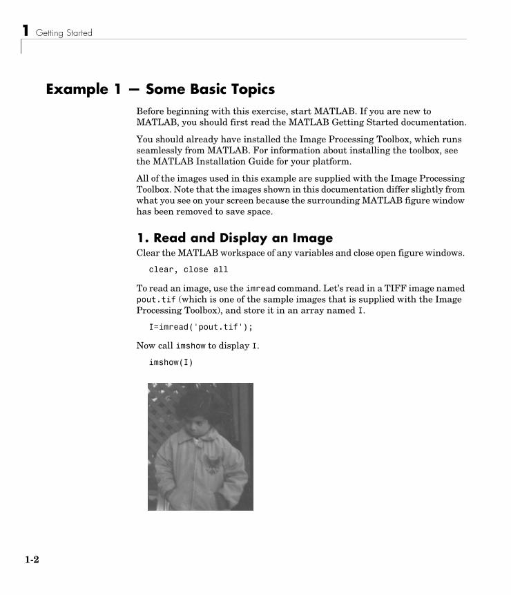
To read an image, use the imread command. Let’s read in a TIFF image named pout.tif (which is one of the sample images that is supplied with the Image Processing Toolbox), and store it in an array named I.

I=imread('pout.tif');

Now call imshow to display I.

imshow(I)

Example 1 — Some Basic Topics

1-3

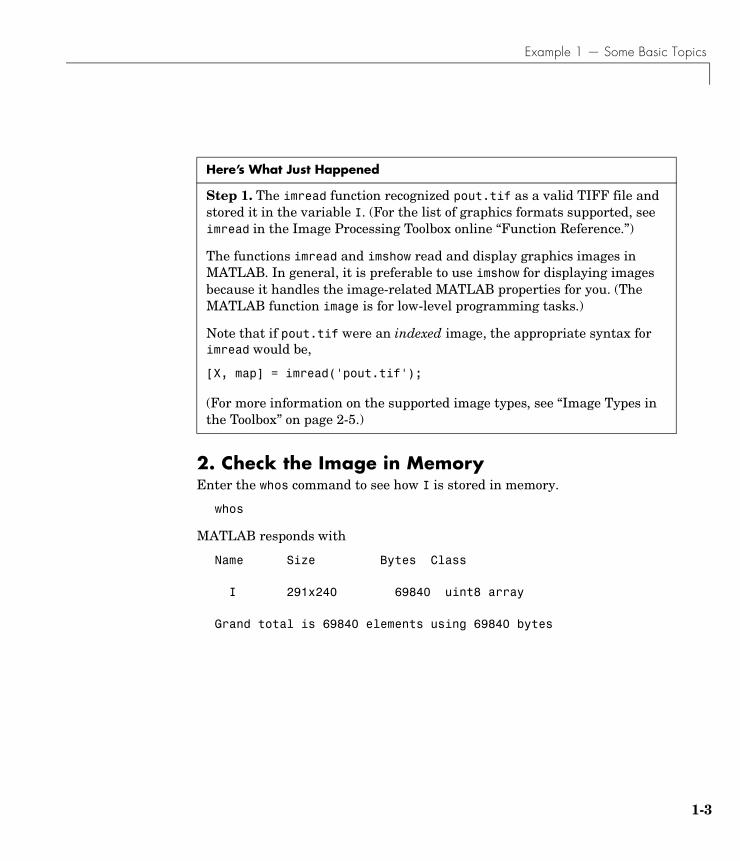
2. Check the Image in MemoryEnter the whos command to see how I is stored in memory.

whos

MATLAB responds with

Name Size Bytes Class

I 291x240 69840 uint8 array

Grand total is 69840 elements using 69840 bytes

Here’s What Just Happened

Step 1. The imread function recognized pout.tif as a valid TIFF file and stored it in the variable I. (For the list of graphics formats supported, see imread in the Image Processing Toolbox online “Function Reference.”)

The functions imread and imshow read and display graphics images in MATLAB. In general, it is preferable to use imshow for displaying images because it handles the image-related MATLAB properties for you. (The MATLAB function image is for low-level programming tasks.)

Note that if pout.tif were an indexed image, the appropriate syntax for imread would be,

[X, map] = imread('pout.tif');

(For more information on the supported image types, see “Image Types in the Toolbox” on page 2-5.)

1 Getting Started

1-4

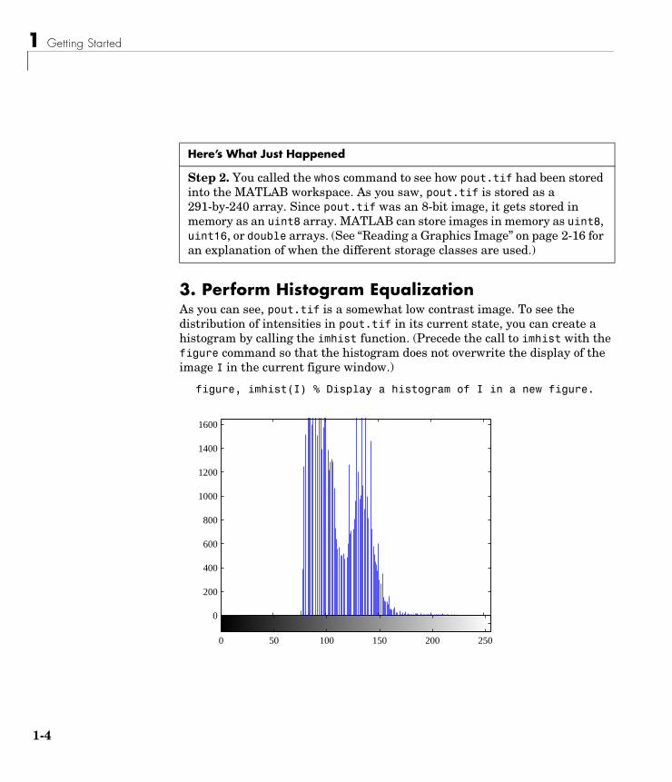
3. Perform Histogram EqualizationAs you can see, pout.tif is a somewhat low contrast image. To see the distribution of intensities in pout.tif in its current state, you can create a histogram by calling the imhist function. (Precede the call to imhist with the figure command so that the histogram does not overwrite the display of the image I in the current figure window.)

figure, imhist(I) % Display a histogram of I in a new figure.


Step 2. You called the whos command to see how pout.tif had been stored into the MATLAB workspace. As you saw, pout.tif is stored as a 291-by-240 array. Since pout.tif was an 8-bit image, it gets stored in memory as an uint8 array. MATLAB can store images in memory as uint8, uint16, or double arrays. (See “Reading a Graphics Image” on page 2-16 for an explanation of when the different storage classes are used.)

0 50 100 150 200 250

0

200

400

600

800

1000

1200

1400

1600


1-5

Notice how the intensity range is rather narrow. It does not cover the potential range of [0, 255], and is missing the high and low values that would result in good contrast.

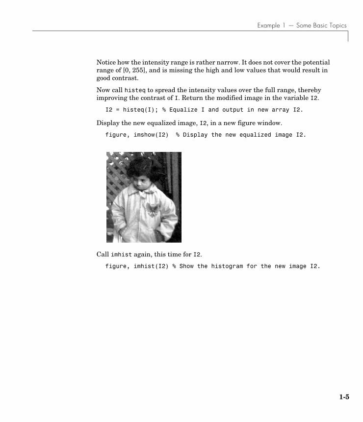
Now call histeq to spread the intensity values over the full range, thereby improving the contrast of I. Return the modified image in the variable I2.

I2 = histeq(I); % Equalize I and output in new array I2.

Display the new equalized image, I2, in a new figure window.

figure, imshow(I2) % Display the new equalized image I2.

Call imhist again, this time for I2.

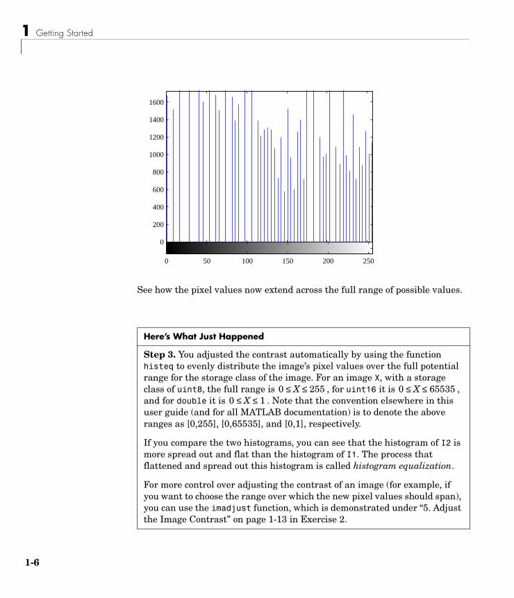
figure, imhist(I2) % Show the histogram for the new image I2.

1 Getting Started

1-6

See how the pixel values now extend across the full range of possible values.


Step 3. You adjusted the contrast automatically by using the function histeq to evenly distribute the image’s pixel values over the full potential range for the storage class of the image. For an image X, with a storage class of uint8, the full range is , for uint16 it is , and for double it is . Note that the convention elsewhere in this user guide (and for all MATLAB documentation) is to denote the above ranges as [0,255], [0,65535], and [0,1], respectively.

If you compare the two histograms, you can see that the histogram of I2 is more spread out and flat than the histogram of I1. The process that flattened and spread out this histogram is called histogram equalization.

For more control over adjusting the contrast of an image (for example, if you want to choose the range over which the new pixel values should span), you can use the imadjust function, which is demonstrated under “5. Adjust the Image Contrast” on page 1-13 in Exercise 2.

0 50 100 150 200 250

0

200

400

600

800

1000

1200

1400

1600

0 X 255≤ ≤ 0 X 65535≤ ≤0 X 1≤ ≤


1-7

4. Write the ImageWrite the newly adjusted image I2 back to disk. Let’s say you’d like to save it as a PNG file. Use imwrite and specify a filename that includes the extension 'png'.

imwrite (I2, 'pout2.png');

5. Check the Contents of the Newly Written FileNow, use the imfinfo function to see what was written to disk. Be sure not to end the line with a semicolon so that MATLAB displays the results. Also, be sure to use the same path (if any) as you did for the call to imwrite, above.

imfinfo('pout2.png')


ans =


Step 4. MATLAB recognized the file extension of 'png' as valid and wrote the image to disk. It wrote it as an 8-bit image by default because it was stored as a uint8 intensity image in memory. If I2 had been an image array of type RGB and class uint8, it would have been written to disk as a 24-bit image. If you want to set the bit depth of your output image, use the BitDepth parameter with imwrite. This example writes a 4-bit PNG file.

imwrite(I2, 'pout2.png', 'BitDepth', 4);

Note that all output formats do not support the same set of output bit depths. See imwrite in the Reference for the list of valid bit depths for each format. See also “Writing a Graphics Image” on page 2-17 for a tutorial discussion on writing images using the Image Processing Toolbox.

Filename:'pout2.png'FileModDate:'03-Jun-1999 15:50:25'

FileSize:36938Format:'png'

FormatVersion:[]

1 Getting Started

1-8

. . .

Note This example shows only a subset of all the fields returned by imfinfo. Also, the value in the FileModDate field for your file will be different from what is shown above. It will show the date and time that you used imwrite to create your image.

Width:240Height:291

BitDepth:8ColorType:'grayscale'


Step 5. When you called imfinfo, MATLAB displayed all of the header fields for the PNG file format that are supported by the toolbox. You can modify many of these fields by using additional parameters in your call to imwrite. The additional parameters that are available for each file format are listed in tables in the reference entry for imwrite. (See “Querying a Graphics File” on page 2-18 for more information about using imfinfo.)

Example 2 — Advanced Topics

1-9

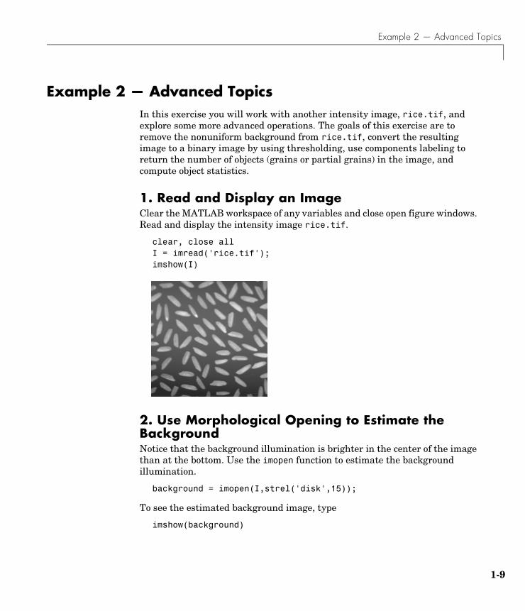
Example 2 — Advanced TopicsIn this exercise you will work with another intensity image, rice.tif, and explore some more advanced operations. The goals of this exercise are to remove the nonuniform background from rice.tif, convert the resulting image to a binary image by using thresholding, use components labeling to return the number of objects (grains or partial grains) in the image, and compute object statistics.

1. Read and Display an ImageClear the MATLAB workspace of any variables and close open figure windows. Read and display the intensity image rice.tif.

clear, close allI = imread('rice.tif');imshow(I)

2. Use Morphological Opening to Estimate the BackgroundNotice that the background illumination is brighter in the center of the image than at the bottom. Use the imopen function to estimate the background illumination.

background = imopen(I,strel('disk',15));

To see the estimated background image, type

imshow(background)

1 Getting Started

1-10

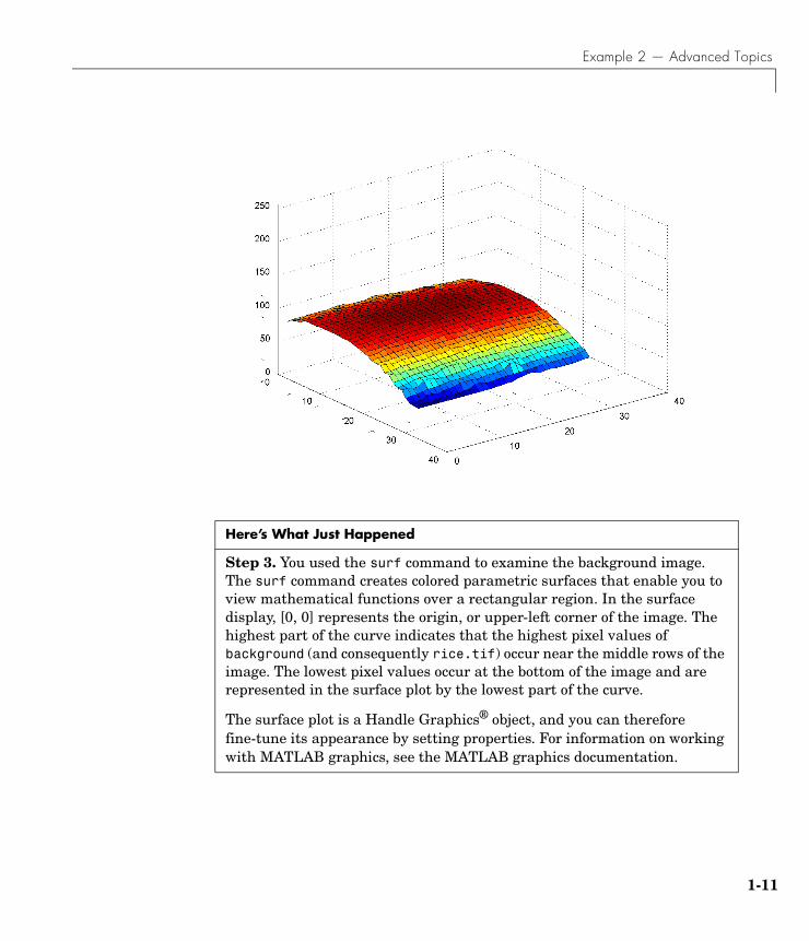
3. Display the Background Approximation as a SurfaceUse the surf command to create a surface display of the background approximation, background. The surf function requires data of class double, however, so you first need to convert background using the double command.

figure, surf(double(background(1:8:end,1:8:end))),zlim([0 255]);set(gca,'ydir','reverse');

The example uses MATLAB indexing syntax to view only 1 out of 8 pixels in each direction; otherwise the surface plot would be too dense. The example also sets the scale of the plot to better match the range of the uint8 data and reverses the y-axis of the display to provide a better view of the data (the pixels at the bottom of the image appear at the front of the surface plot).


Step 1. You used the toolbox functions imread and imshow to read and display an 8-bit intensity image. imread and imshow are discussed in Exercise 1, in “2. Check the Image in Memory” on page 1-3, under the “Here’s What Just Happened” discussion.

Step 2. You performed a morphological opening operation by calling imopen with the input image, I, and a disk-shaped structuring element with a radius of 15. The structuring element was created by the strel function. The morphological opening has the effect of removing objects that cannot completely contain a disk of radius 15. For more information about morphological opening, see Chapter 9, “Dilation- and Erosion-Based Functions.”


1-11


Step 3. You used the surf command to examine the background image. The surf command creates colored parametric surfaces that enable you to view mathematical functions over a rectangular region. In the surface display, [0, 0] represents the origin, or upper-left corner of the image. The highest part of the curve indicates that the highest pixel values of background (and consequently rice.tif) occur near the middle rows of the image. The lowest pixel values occur at the bottom of the image and are represented in the surface plot by the lowest part of the curve.

The surface plot is a Handle Graphics® object, and you can therefore fine-tune its appearance by setting properties. For information on working with MATLAB graphics, see the MATLAB graphics documentation.

1 Getting Started

1-12

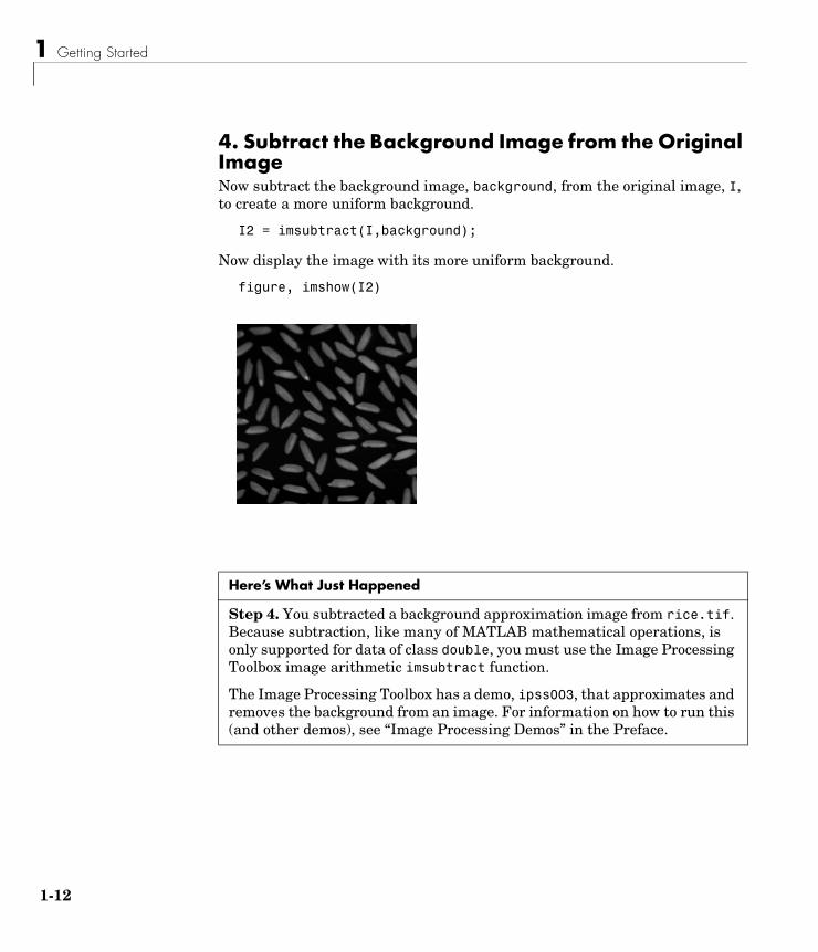
4. Subtract the Background Image from the Original ImageNow subtract the background image, background, from the original image, I, to create a more uniform background.

I2 = imsubtract(I,background);

Now display the image with its more uniform background.

figure, imshow(I2)


Step 4. You subtracted a background approximation image from rice.tif. Because subtraction, like many of MATLAB mathematical operations, is only supported for data of class double, you must use the Image Processing Toolbox image arithmetic imsubtract function.

The Image Processing Toolbox has a demo, ipss003, that approximates and removes the background from an image. For information on how to run this (and other demos), see “Image Processing Demos” in the Preface.


1-13

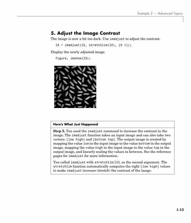
5. Adjust the Image ContrastThe image is now a bit too dark. Use imadjust to adjust the contrast.

I3 = imadjust(I2, stretchlim(I2), [0 1]);

Display the newly adjusted image.

figure, imshow(I3);


Step 5. You used the imadjust command to increase the contrast in the image. The imadjust function takes an input image and can also take two vectors: [low high] and [bottom top]. The output image is created by mapping the value low in the input image to the value bottom in the output image, mapping the value high in the input image to the value top in the output image, and linearly scaling the values in between. See the reference pages for imadjust for more information.

You called imadjust with stretchlim(I2) as the second argument. The stretchlim function automatically computes the right [low high] values to make imadjust increase (stretch) the contrast of the image.

1 Getting Started

1-14

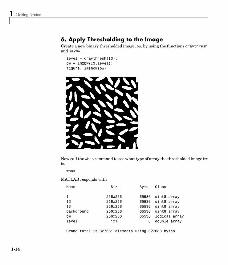
6. Apply Thresholding to the ImageCreate a new binary thresholded image, bw, by using the functions graythresh and im2bw.

level = graythresh(I3);bw = im2bw(I3,level); figure, imshow(bw)

Now call the whos command to see what type of array the thresholded image bw is.

whos



I 256x256 65536 uint8 arrayI2 256x256 65536 uint8 arrayI3 256x256 65536 uint8 arraybackground 256x256 65536 uint8 arraybw 256x256 65536 logical arraylevel 1x1 8 double array



1-15

7. Determine the Number of Objects in the ImageTo determine the number of grains of rice in the image, use the bwlabel function. This function labels all of the connected components in the binary image bw and returns the number of objects it finds in the image in the output value, numobjects.

[labeled,numObjects] = bwlabel(bw,4);% Label components.

numObjects =

80

The accuracy of your results depends on a number of factors, including:

• The size of the objects

• The accuracy of your approximated background

• Whether you set the connectivity parameter to 4 or 8

• Whether or not any objects are touching (in which case they may be labeled as one object) In the example, some grains of rice are touching, so bwlabel treats them as one object.


Step 6. You called graythresh to automatically compute an appropriate threshold to use to convert the intensity image to binary. You then called im2bw to perform for thresholding, using the threshold, level, returned by graythresh.

Notice that when you call the whos command, you see the expression logical listed after the class for bw. This indicates the presence of a logical flag. The flag indicates that bw is a logical matrix, and the Image Processing Toolbox treats logical matrices as binary images. Thresholding using MATLAB logical operators always results in a logical image. For more information about binary images and the logical flag, see “Binary Images” on page 2-8.

1 Getting Started

1-16

8. Examine the Label MatrixYou may find it helpful to take a closer look at labeled to see what bwlabel has created. Use the imcrop command to select and display pixels in a region of labeled that includes an object and some background.

To ensure that the output is displayed in the MATLAB window, do not end the line with a semicolon. In addition, choose a small rectangle for this exercise, so that the displayed pixel values don’t wrap in the MATLAB command window.

The syntax shown below makes imcrop work interactively. Your mouse cursor becomes a cross-hair when placed over the image. Click at a position in labeled where you would like to select the upper left corner of a region. Drag the mouse to create the selection rectangle, and release the button when you are done.

grain = imcrop(labeled) % Crop a portion of labeled.

We chose the left edge of a grain and got the following results.

grain =


Step 7. You called bwlabel to search for connected components and label them with unique numbers. bwlabel takes a binary input image and a value specifying the connectivity of objects. The parameter 4, passed to the bwlabel function, means that pixels must touch along an edge to be considered connected. For more information about the connectivity of objects, see “Pixel Connectivity” in Chapter 9.

You can also determine the number of objects in a label matrix by asking for the maximum pixel value in the image. For example,

max(labeled(:))

ans =

80


1-17

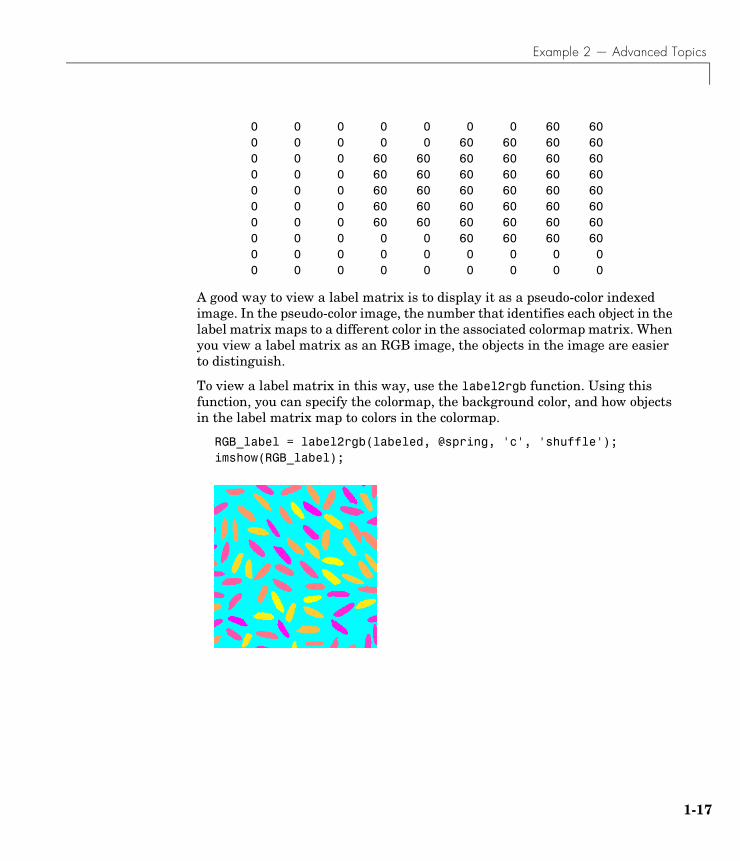
0 0 0 0 0 0 0 60 60 0 0 0 0 0 60 60 60 60 0 0 0 60 60 60 60 60 60 0 0 0 60 60 60 60 60 60 0 0 0 60 60 60 60 60 60 0 0 0 60 60 60 60 60 60 0 0 0 60 60 60 60 60 60 0 0 0 0 0 60 60 60 60 0 0 0 0 0 0 0 0 0 0 0 0 0 0 0 0 0 0

A good way to view a label matrix is to display it as a pseudo-color indexed image. In the pseudo-color image, the number that identifies each object in the label matrix maps to a different color in the associated colormap matrix. When you view a label matrix as an RGB image, the objects in the image are easier to distinguish.

To view a label matrix in this way, use the label2rgb function. Using this function, you can specify the colormap, the background color, and how objects in the label matrix map to colors in the colormap.

RGB_label = label2rgb(labeled, @spring, 'c', 'shuffle');imshow(RGB_label);

1 Getting Started

1-18

9. Measure Object Properties in the ImageThe regionprops command measures object or region properties in an image and returns them in a structure array. When applied to an image with labeled components, it creates one structure element for each component. Use regionprops to create a structure array containing some basic properties for labeled.

graindata = regionprops(labeled,'basic')



Step 8. You called imcrop and selected a portion of the image that contained both some background and part of an object. The pixel values were returned in the MATLAB window. If you examine the results above, you can see the corner of an object labeled with 60’s, which means that it was the 60th object labeled by bwlabel.

The imcrop function can also take a vector specifying the coordinates for the crop rectangle. In this case, it does not operate interactively. For example, this call specifies a crop rectangle whose upper-left corner begins at (15, 25) and has a height and width of 10.

rect = [15 25 10 10];roi = imcrop(labeled, rect)

You are not restricted to rectangular regions of interest. The toolbox also has a roipoly command that enables you to select polygonal regions of interest. Many image processing operations can be performed on regions of interest, including filtering and filling. See Chapter 11, “Region-Based Processing” for more information.

The call to label2rgb illustrates a good way to visualize label matrices. The pixel values in the label matrix are used as indices into a colormap. Using label2rgb, you can specify your own colormap or use one of the MATLAB colormap-creating functions, including gray, pink, spring, and hsv. For information on these functions, see colormap in the MATLAB Function Reference.


1-19

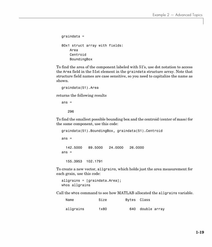
graindata =

80x1 struct array with fields: Area Centroid BoundingBox

To find the area of the component labeled with 51’s, use dot notation to access the Area field in the 51st element in the graindata structure array. Note that structure field names are case sensitive, so you need to capitalize the name as shown.

graindata(51).Area

returns the following results

ans =

296

To find the smallest possible bounding box and the centroid (center of mass) for the same component, use this code:

graindata(51).BoundingBox, graindata(51).Centroid

ans =

142.5000 89.5000 24.0000 26.0000ans =

155.3953 102.1791

To create a new vector, allgrains, which holds just the area measurement for each grain, use this code:

allgrains = [graindata.Area];whos allgrains

Call the whos command to see how MATLAB allocated the allgrains variable.


allgrains 1x80 640 double array

1 Getting Started

1-20


allgrains is a one-row array of 80 elements, where each element contains the area measurement of a grain. Check the area of the 51st element of allgrains.

allgrains(51)

returns

ans =

296

which is the same result that you received when using dot notation to access the Area field of graindata(51).


Step 9. You called regionprops to return a structure of basic property measurements for each thresholded grain of rice. The regionprops function supports many different property measurements, but setting the properties parameter to 'basic' is a convenient way to return three of the most commonly used measurements: the area, the centroid (or center of mass), and the bounding box. The bounding box represents the smallest rectangle that can contain a region, or in this case, a grain. The four-element vector returned by the BoundingBox field,

[142.5000 89.5000 24.0000 26.0000]

shows that the upper left corner of the bounding box is positioned at [142.5 89.5], and the box has a width of 24.0 and a height of 26.0. (The position is defined in spatial coordinates, hence the decimal values. For more information on the spatial coordinate system, see “Spatial Coordinates” on page 2-29.) For more information about working with MATLAB structure arrays, see “Structures” in the MATLAB programming and data types documentation.

You used dot notation to access the Area field of all of the elements of graindata and stored this data to a new vector allgrains. This step simplifies analysis made on area measurements because you do not have to use field names to access the area.


1-21

10. Compute Statistical Properties of Objects in the ImageNow use MATLAB functions to calculate some statistical properties of the thresholded objects. First use max to find the size of the largest grain. (If you have followed all of the steps in this exercise, the “largest grain” is actually two grains that are touching and have been labeled as one object).

max(allgrains)

returns

ans =

695

Use the find command to return the component label of this large-sized grain.

biggrain = find(allgrains==695)

returns

biggrain =

68

Find the mean grain size.

mean(allgrains)

returns

ans =

249

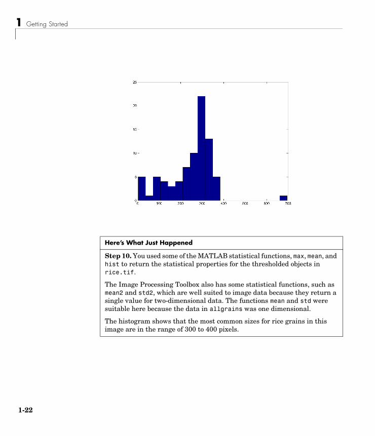
Make a histogram containing 20 bins that show the distribution of rice grain sizes.

hist(allgrains,20)

1 Getting Started

1-22


Step 10. You used some of the MATLAB statistical functions, max, mean, and hist to return the statistical properties for the thresholded objects in rice.tif.

The Image Processing Toolbox also has some statistical functions, such as mean2 and std2, which are well suited to image data because they return a single value for two-dimensional data. The functions mean and std were suitable here because the data in allgrains was one dimensional.

The histogram shows that the most common sizes for rice grains in this image are in the range of 300 to 400 pixels.

Where to Go from Here

1-23

Where to Go from HereFor more information about the topics covered in these exercises, read the tutorial chapters that make up the remainder of this documentation. For reference information about any of the Image Processing Toolbox functions, see the online “Function Reference”, which complements the M-file help that is displayed in the MATLAB command window when you type

help functionname

For example,

help imshow

Online HelpThe Image Processing Toolbox User’s Guide is available online in both HTML and PDF formats. To access the HTML help, select Help from the menu bar of the MATLAB desktop. In the Help browser, expand the Image Processing Toolbox topic in the list. To access the PDF help, click on Image Processing Toolbox in the Contents tab of the Help browser, and go to the link under “Printable Documentation (PDF).” (Note that to view the PDF help, you must have Adobe's Acrobat Reader installed.)

Toolbox DemosThe Image Processing Toolbox includes many demo applications. The demos are useful for seeing the toolbox features put into action and for borrowing code for your own applications. See “Image Processing Demos” in the Preface for a complete list and summary of the demos, as well as instructions on how to run them.

1 Getting Started

1-24

Image Processing Toolbox -...

Documents

Transcript of Image Processing Toolbox -...