IMAGE PROCESSING TECHNIQUES

TO IDENTIFY PREDATORY BIRDS IN AQUACULTURAL SETTINGS

A Thesis Submitted to the Graduate Faculty of the

Louisiana State University and Agricultural and Mechanical College

in partial fulfillment of the requirements for the degree of

Master of Science in Biological and Agricultural Engineering

in

The Department of Biological and Agricultural Engineering

By Uma Devi Nadimpalli

B.E. Andhra University Visakhapatnam, India, 2002

May, 2005

ACKNOWLEDGEMENTS

This thesis would not have been possible without the assistance from many people who

gave their support in different ways. First of all, I would like to express my sincere

gratitude to my advisors, Dr. Randy Price and Dr. Steven Hall, for their invaluable

guidance and encouragement extended through out the study. I also thank Dr. Marybeth

Lima and Dr. Chandra Theegala for serving on my graduate committee. I would like to

thank my friend, Ms. Pallavi Bomma, and other colleagues and friends at LSU for their

constant help and valuable suggestions throughout the study. I would also thank Prof.

Mark Claesgens, from the department of Ag Communications for providing me few

pictures of birds. I am grateful to my parents, Mr. and Mrs. Rama Raju, and my brother,

for the tremendous amount of inspiration and moral support they have given me.

Last but not the least, I would like to gratefully acknowledge the project support from the

Department of Biological and Agricultural Engineering, Louisiana State University

Agricultural Center.

ii

TABLE OF CONTENTS

ACKNOWLEDGMENTS………………………………...……………………………. ii LIST OF TABLES…………………………………………………...………………..... v LIST OF FIGURES…………………………………………...……………….………..vi ABSTRACT………………………………………………………...…………………Viii CHAPTER 1: INTRODUCTION……………………………………………………….1

CHAPTER 2: BACKGROUND AND LITERATURE REVIEW………………........7 2.1 Autonomous Vehicles…………………….…………………………………….…......7 2.2 Image Processing……………………………………………………………………...8 2.3 Autonomous Vehicles Using Image Processing…………………...……………….....9 2.4 Object Recognition Methods………………………………….……………………11 2.4.1 Gray Level Thresholding……………………...…………………………...14 2.4.2 Color Thresholding…………………...……………………………………16

2.4.2.1 RGB Thresholding………………………...…………………......16 2.4.2.2 HSV Thresholding…………………………………...………......18

2.4.3 Size Threshold…………………………………………………………......20 2.4.4 Dilation……………………………………………………….....................21 2.4.5 Artificial Neural Networks…………………………………………...……22 2.4.6 Template Matching………………………………………………………...24 2.4.7 Other Methods…………………………………………………..................25

CHAPTER 3: IMPLEMENTATION METHODOLOGY.………………………….28 3.1 Image Morphology…..………………………...…………………………………......30

3.1.1 Acquire an Input Image….…………………...……………………………31 3.1.2 Convert Input Images to Different Color Spaces…………………………..32 3.1.3 Remove Horizon Pixels…………………….……………………………...34 3.1.4 Add Required Rows and Columns…………………………………………35 3.1.5 Local Thresholding………………………………………………………...36 3.1.6 Convert Image to Gray Scale………………………………………………37 3.1.7 Size Threshold…………………………………………………………......37 3.1.8 Remove Rows and Columns……………………………………………….39 3.1.9 Dilation………………………………………………………………….....39

3.2 Artificial Neural Networks…………………………………………………………..39 3.2.1 Log Sigmoid Function……………………………………………………..42 3.2.2 ANN Algorithm……………………………………………………………42

3.3 Template Matching ………………………………………………………………….44 3.4 Real Time Algorithm to Control Autonomous Boat…………………………………47

iii

CHAPTER 4: RESULTS AND DISCUSSION ………………………………………50 4.1 Image Morphology………..………………………………………………….………50 4.1.1 Pelicans…………………………………………………………….………50 4.1.2 Egrets………………………………………………………………………52 4.1.3 Cormorants…………………………………………………………………52 4.2 Artificial Neural Networks…………………………………………………………..54 4.3 Template Matching ……………………………………………………………….....55 4.3.1 Pelicans and Egrets………………………………………………………...56 4.3.2 Cormorants…………………………………………………………………62 CHAPTER 5: CONCLUSIONS AND RECOMMENDATIONS FOR THE FUTURE...........................................................................................................................65 REFERENCES…………………………………………………………………………68 APPENDIX A IMAGE PROCESSING ALGORITHMS………………......………..76 APPENDIX B PAST RESEARCH ON OBJECT RECOGNITION ……...…..……96 APPENDIX C IMAGE PROCESSING TECHNIQUES FOR RECOGNITION OF BIRDS IN AQUACULTURAL SETTINGS…………………………………………..98 VITA……………………………………………...……………………………………120

iv

LIST OF TABLES 4.1 Results obtained by testing image morphology algorithm on all types of images……………………………………………………………………………………51 4.2 Tabulated results from ANN algorithm…..……...…………………………………..55 4.3 Template matching results on pelicans and egrets……...……………………………57 4.4 Template matching results on cormorants………...…………………………………62 Ac.1 Image morphology results…………………….…………………………………..109 Ac.2 Template matching results…………………………...…………………………...113

v

LIST OF FIGURES

1.1 Structure of an artificial neural network model……………………………………….5 2.1 Autonomous boat built by LSU Agricultural Center………………………………...10 2.2 Images having eight and four connected neighborhood pixels………………………12 3.1 Types of images……………………………………………………………………...29 3.2 Input image to image morphology algorithm……………......………………………31 3.3 Input images…………………………………………………...………………...…..33 3.4 Images after cutting 100 rows of sky pixels……………………....…………………35

3.5 Input RGB image after cutting sky pixel rows and addition of required rows and columns……………...………………………………………………………………...…36 3.6 Flow chart representing image morphology……………………...………………….38 3.7 A generalized model of an artificial neural network………………...……………....40 3.8 Log sigmoid activation function……………………………………...……………...41 3.9 Template matching technique…………………………………………...…………...45 3.10 Model of the template matching technique used in the study………….…………...46 3.11 Flow chart explaining the template matching technique……………….………......48 3.12 Block diagram for the control of autonomous boat…………………….………......49 4.1 Results from the ANN algorithm…………………………………………...………..54 4.2 Results obtained while testing Type 1 images of pelicans and egrets………...…......59 4.3 Results obtained while testing Type 2 images of pelicans and egrets………….........59 4.4 Results obtained while testing Type 3 images of pelicans and egrets………….........60 4.5 Operation time for testing images using template matching…………………........61 4.6 Results obtained while testing Type 1 images of cormorants …………………........63 4.7 Results obtained while testing Type 2 images of cormorants …………………........64

vi

4.8 Results obtained while testing Type 3 images of cormorants…………………….....64 Ac.1 A generalized model of an artificial neural network……………………………...105 Ac.2 The template matching technique………………………………………………...107 Ac.3 Image morphology on Type 3 images…………………………………………….111 Ac.4 Images after testing morphology algorithm on Type 3 images…………………...111

vii

ABSTRACT

Bird predation is a major problem in aquaculture. A novel method for dispersing

birds is the use of a vehicle that can sense and chase birds. Image recognition software

can improve their efficiency in chasing birds. Three recognition techniques were tested to

identify birds 1) image morphology 2) artificial neural networks, and 3) template

matching have been tested. A study was conducted on three species of birds 1) pelicans,

2) egrets, and 3) cormorants. Images were divided into 3 types 1) Type 1, 2) Type 2, and

3) Type 3 depending upon difficulty to separate from the others in the images. These

types were clear, medium clear and unclear respectively. Image morphology resulted in

57.1% to 97.7%, 73.0% to 100%, and 46.1% to 95.5% correct classification rates (CCR)

respectively on images of pelicans, cormorants and egrets before size thresholding. The

artificial neural network model achieved 100% CCR while testing type 1 images and its

classification success ranged from 63.5% to 70.0%, and 57.1% to 67.7% while testing

type 2 and type 3 images respectively. The template matching algorithm succeeded in

classifying 90%, 80%, and 60% of Type 1, Type 2 and Type 3 images of pelicans and

egrets. This technique recognized 80%, 91.7%, and 80% of Type 1, Type 2, and Type 3

images of cormorants.

We developed a real time recognition algorithm that could capture images from a

camera, process them, and send output to the autonomous boat in regular intervals of

time. Future research will focus on testing the recognition algorithms in natural or

aquacultural settings on autonomous boats.

viii

CHAPTER 1: INTRODUCTION

Louisiana is ranked as one of the biggest fish producers in the United States.

Louisiana has a variety of fresh water fisheries and is the largest producer of crawfish and

oysters in the entire United States. One-fourth’s of the total seafood in the United States

comes from Louisiana (Harvey, 1998).

Louisiana is also famous for a wide variety of bird species. Louisiana is called the

“pelican state” because of enormous number of pelicans found along the coast (Harvey,

1998). These birds along with other birds such as egrets, herons and cormorants cause

much damage to the fish population in a pond. Heavy losses to the aquacultural farmers

have been reported due to the bird predation. Bird predation on fish has become a

significant concern for aquacultural farmers over the past few years. Significant

investment is being made to find ways to save fish from predatory birds.

Scott. (2002) estimated that the aquaculture industry has been investing about $17

million annually on bird damage and damage prevention. If one cormorant eats 1 lb of

fish per day, 2 million birds can have a very large impact if they foraged exclusively on

aquaculture facilities. During an average winter in the delta region of Mississippi, losses

to the catfish industry alone can be $5 million dollars in lost fish due to cormorant

predation (Glahn et al., 1995, 2000). Littauer et al. (1997) stated that one egret could eat

31 pound of fish per day, while a great heron can eat 3

2 to 43 pound per day. Though

cormorants weigh only 4 pounds, they can consume up to one pound of fish on an

average per day (Anonymous, 2004). Pelicans can consume 1 to 3 pounds of fish per day.

Stickley et al. (1989) estimated that catfish losses in 1988 amounted to $3.3 million due

1

to double-crested cormorants. Thus reducing the predation of birds on fish is the sole way

to increase the yield of fish and protect the farming community.

A huge sum of money is being spent to stop these fast breeding predators. Several

methods such as shooting and poisoning were ineffective or unfriendly to the

environment (Hall et al., 2001). Another way to reduce the predation of birds is to use

sonic cannons, but birds may get accustomed to the loud noises over time (Bomford et

al., 1990). Also the sonic cannons can cause local sound pollution. Some birds such as

the double crested cormorants, American white pelican, brown pelican, and great egret,

etc are either protected or endangered species according to the Migratory Bird Treaty

Act. (1918) and Endangered Species Act. (1973), and should not be killed. Shooting and

feeding these species of birds would be against the federal law.

Since many methods that were used in the past are not effective in reducing the

bird predation, there is a need for switching to other approaches of reducing the bird

predation. One such approach is the use of autonomous vehicles. A robotic system that

emulates a human worker could be the best possible alternative for the automation of

agricultural operations. This is a novel concept taking into consideration the recent

development of computers, sensor technology, and the application of artificial

intelligence (Bulanon et al., 2001). An autonomous robotic system means that the system

will be able to work continuously, on its own, without any external help. These vehicles

can go to dangerous places, like an atomic reactor, which cannot normally be reached by

humans. Also, automation of agricultural tasks makes it cost effective to reduce labor

costs, saving time as human power is replaced by machines.

2

An autonomous vehicle, such as a boat, which can detect birds and disperse them

without human intervention would be a good solution to bird predation problem.

Software programs and camera systems could be mounted on autonomous vehicles to

detect birds. These systems can provide safe, reliable, maintenance-free, and

environmentally friendly ways to detect birds.

An overall study of the environmental issues, economic conditions, and other

problems led to the development of autonomous devices. Price et al. (2001) designed an

autonomous scare boat that chases birds away from the lake. This semi autonomous boat

works on solar power, and is also being used to track water quality parameters such as

dissolved oxygen, temperature, BOD (biochemical oxygen demand) etc. A machine

vision system was developed to recognize birds and worked satisfactorily in the

laboratory, but could not cover all situations in the field. Problems with the system

included intense sunlight, and many colors variations of the birds as well as the motion of

the platform. These problems result in the need for image processing algorithms that will

operate under all conditions. Developing image processing algorithms for autonomous

boats would help in the accurate detection and tracking of the birds.

The objectives of my study are to

1) Recognize the birds using image morphology and artificial neural networks.

2) Develop a real time algorithm that could be used by an autonomous boat to disperse

birds.

We implemented all image-processing algorithms using the image processing and

neural network tool boxes of the popular software MATLAB® 6.5 (Math Works, 2005).

The main advantage with using this software is spending less time on debugging and

3

coding the program compared to other programming languages such as ‘C’,’C++’ and

FORTRAN. MATLAB® 6.5 has several built in functions in the image processing

toolbox which makes the user easy to understand, implement and decode. Three

algorithms 1) image morphology, 2) artificial neural networks, and 3) template matching

have been designed. Several researchers have worked on object recognition in the past.

Chapter 2 provided an overview of these methods used for object recognition in the past.

Image morphology is the step by step method of extracting useful information

from the image. Some steps include removing the pixels above the water surface,

thresholding based on the intensity, size. Finally, we divide the image into 3 vertical

sections and use these sections to locate birds and telling the boat which way to turn.

Chapter 3 focuses on detailed description of every step in this algorithm and chapter 4

concentrates on the results and discussions obtained using the algorithm.

A neural network (Figure 1.1) has been developed using the MATLAB® 6.5

(Math Works, 2005) neural network toolbox. This network typically consists of many

hundreds of processing units called neurons which are wired together in a complex

communication network. Each unit or node is a simplified model of a real neuron which

fires (sends off a new signal) if it receives a sufficiently strong input signal from the other

nodes to which it is connected. The strength of these connections may be varied in order

for the network to perform different tasks corresponding to different patterns of node

firing activity. This structure is very different from traditional computers. These

programs simulate the performance of the brain although the brains network has still not

been fully understood (Anonymous, 2003). Details of the algorithm are presented in

chapter 3.

4

p1

p2

p3

p4

N11

N12

N13

N14

N21

N23

N22

N24

b13

b11

b12

b14

w111

w112

w113

w114

w141

w142

w143

w144

a1

a3

a2

a4

f11

f14

f13

f12

w211

w213

w214

w212

w2411

w242

w24 3

w24 4

b23

b22

b21

b24

f21

f24

f23

f22Log

sigmoid

∫ Output

Threshold

p1

p2

p3

p4

N11

N12

N13

N14

N21

N23

N22

N24

b13

b11

b12

b14

w111

w112

w113

w114

w141

w142

w143

w144

a1

a3

a2

a4

f11

f14

f13

f12

w211

w213

w214

w212

w2411

w242

w24 3

w24 4

b23

b22

b21

b24

f21

f24

f23

f22Log

sigmoid

∫ Output

Threshold

Figure: 1.1. Structure of an artificial neural network model

Another method that has gained popularity in recent years is object recognition

using template matching. This method compares an input image with a standard set of

images, known as templates. For bird identification templates are bird parts cut from

various pictures. A threshold correlation value is determined and if the correlation

between the template and the input image is above the threshold value then the input

image is considered to have birds. Accurate recognition of birds requires the use of

multiple template images since template matching is not invariant to rotation, size, etc.

Template matching is the last object recognition method implemented in this project and

is presented in chapter 3.

5

Correct classification rate (CCR) and misclassification rate (MCR) are calculated

for each species of birds using the three algorithms. CCR is birds recognized divided by

birds present in the image. MCR is non-birds recognized divided by total objects

recognized in the image. Results are tabulated in chapter 4.

In order to meet the second objective, an image processing algorithm has been

developed for real time use on the autonomous boat built by Price and Hall (Price, and

Hall (2000, 2002), Hall and Price (2003 a, b, c), and Hall et al (2001, 2004, 2005)).

Methods used to automate the algorithms in real time have been included in the chapter 3.

Field experiments will be done in the future on variety of birds, such as pelicans, egrets,

cormorants and herons, which are the major predators. We have included conclusions,

and recommendations for future research in chapter 5.

6

CHAPTER 2: BACKGROUND AND LITERATURE REVIEW

Louisiana is famous for a variety of birds that live in colonies and prey on fish.

Famous among them are the double crested cormorants, pelicans, egrets that hunt

individually or in flocks. These birds dive deep, swim under the water, and are capable of

catching many fish at a time. Louisiana aquacultural farms are suffering from rapid

decrease of fish due to these birds. Killing these birds would not be a good idea as some

of these birds come under the category of endangered or protected species according to

endangered species act of 1973 and the migratory bird treaty act of 1918. Killing or

poisoning the birds would also pollute the lakes. Preventing birds from consuming fish

may be way of protecting them.

Researchers implemented several different methods such as the use of sonic

cannons and nets in the past but they proved ineffective in reducing bird predation, as

these birds got accustomed to such sounds. Dispersing the birds would require some kind

of recognition software and an autonomous vehicle on which the software designed to

detect birds can be mounted and used to chase birds.

2.1 Autonomous Vehicles

The past few decades have seen the development of autonomous vehicles to serve

different purposes. Autonomous vehicles are being developed that can operate in

dangerous places such as the atomic reactors (Anonymous, 2002). Griepentrog et al.

(2003) developed autonomous vehicle for agricultural field operations such as weeding

and spraying. Simpson et al. (2003) developed an unmanned aerial vehicle (UAV) that

captures remote sensed imagery for precision agriculture. This system captures imagery

7

from various locations with ease. Shallow Water Autonomous Mine Sweeping Initiation

(SWAMS) developed an automatic detection and classification of mines in shallow

water. Blackmore et al. (2002) have developed an autonomous tractor for successful

mechanical weeding and field scouting. According to Graves, (2004) Automatic Milking

Systems (AMS) are being used in many parts of Europe for milking cows with minimal

oversight or intervention. Components included several sensors such as cow

identification, udder/teat location, teat cleanliness and milk flow sensors. Other

components include milking box, power gates, feeding station, udder cleaning, milking

system, milk cooling, and storage. Seipelt et al. (2003) developed a new calf feeder that

solves the problems faced by normal calf feeders such as hygiene, health control and

accuracy of milk location. The Calf feeder has automatic rinsing system and several other

components to indicate the health of the calves.

While some researchers used autonomous vehicles exclusively for object

recognition, other researchers concentrated on image processing techniques.

New challenges in the present application include water, and wind currents and

movement of birds, and the vehicle. In order to seek and track birds, object recognition

using image processing might be considered.

2.2 Image Processing

Several researchers have used image-processing techniques for object recognition.

A series of morphological operations were implemented by Casasent et al. (2001) to

produce only an image of nutmeat from an image containing a number of nuts. Ruiz et al.

(1996) used color segmentation to locate and remove the long stems attached to

mechanically harvested oranges. Their color segmentation algorithm had 100% success

8

in discriminating the destemmed and the stemmed oranges. However, the algorithm

misclassified some pixels of the stem-calyx as background. El-Faki et al. (2000), used

color machine vision for the detection of weeds in wheat and soybean fields. They used a

color index for both the preprocessing and statistical discriminant analysis (DA) for weed

detection. Their experiments worked well with statistical discriminant analysis compared

to the two neural networks they trained. Aitkenhead et al. (2003) used a simple method to

discriminate plants and weeds using plant size as a parameter. They also trained a neural

network to discriminate plants and weeds. Rapid identification of Africanized honeybees

was done by used Batra (1998) using image analysis. Hansen et al. (1997) evaluated

wound status of a porcine animal model, using color image processing. In their

experiment, the differences in calibrated hue between injured and noninjured skin

provided a repeatable differentiation of wound severity for situations when the time of

injury was known.

Although researchers concentrated on both autonomous vehicles and image

processing on an individual basis, few researchers have concentrated on autonomous

vehicles that use image processing.

2.3 Autonomous Vehicles Using Image Processing

The National Institute of Science and Technology (NIST) designed an intelligent

machine that drives on the road at 55 mph. This machine tracks the painted stripes on the

road by using edge detection algorithm (Bostelman, 2002). Kise et al. (2002) are

developing an obstacle detection system for autonomous tractor with steering controller.

Morimoto et al. (2002) developed an obstacle detection system based on HSV image

processing. This autonomous vehicle detects the obstacles in its path and avoids the

9

vehicle from collision. Nishiwaki et al. (2002) developed an autonomous vehicle that

used vision system for estimating plant positions. They calculated yaw angle and vehicle

speed using plant positions estimated using their algorithm.

Most of the research done on autonomous vehicles and image processing

concentrated on plants and its products. Though a number of autonomous vehicles that

operate on ground and in air were developed, very little research has been done on

autonomous vehicles that operate on water. No published research has been done on bird

recognition and the methodologies to scare birds. However, the Biological and

Agricultural Engineering Department at the Louisiana State University developed a semi-

autonomous boat (Fig 2.1) for chasing birds in the lake. One major advantage of this

semi-autonomous boat is that it works on solar power. The power saved during the

daytime can be used by the boat later in the absence of solar power.

Fig: 2.1. Autonomous boat built by LSU Agricultural Center

10

Price and Hall (Price, and Hall (2000, 2002), Hall and Price (2003 a, b, c), and Hall et al

(2001, 2004, 2005)) designed a semi-autonomous boat to reduce the bird predation in

aquacultural ponds. They used a machine vision system designed by Lego Vision

Command TM to identify birds and make the boat chase the birds. Random motion

worked well but chasing birds was a challenge. The software they used breaks the image

into sections using a predetermined grid pattern. Later it trains each section of the image

to detect light, motion or color of the bird that would help in the recognition process.

However, this machine vision system encountered several problems. It worked well in the

laboratory, but when taken outside it faced some problems due to the brightness with

intense sunlight. The machine vision system also had problems calibrating to the white

color of the birds. Therefore, developing image-processing algorithms that work under all

conditions could be the best solution. These algorithms may also reduce unnecessary

wandering of the boat even when no birds are present, which saves on solar power that

can be used later during cloudy or partly sunny conditions. Object recognition algorithms

using built in functions may be the cheapest way. There are different types of object

recognition and researchers have implemented several methods in the past.

2.4 Object Recognition Methods

Recognition is a process of separating the objects of interest from the background.

Recognition becomes simple if the birds are distinct from the surroundings in terms of

color, texture etc. Perhaps the cheapest and easiest way could be the use of a digital

camera to take pictures of the birds and software to recognize the birds in the captured

image. However, in the past very few efforts have been made in the direction of

recognizing birds in a given image. Several methods have been implemented in the past

11

to recognize or discriminate objects such as weeds and plants in an image, which can be

used for recognizing birds. Motion is another challenge in object recognition.

Center Pixel

Eight Connected Four Connected

Center PixelCenter Pixel

Eight Connected Four Connected

Fig: 2.2. Images having eight and four connected neighborhood pixels

Majority of the segmentation procedures developed in the past used CCD (Charge

Couple Devices) to capture images and used local or global (shape) techniques for

recognition. Local approaches use only the values of the neighborhood pixels to calculate

the value of the center pixel. Depending on the application, we consider four or eight

neighborhood pixels (Figure 2.2). Typically, we use 8-connectedness when looking for

objects and 4-connectedness when analyzing the background (Lacey et al., 2004). Local

approaches that used intensity or color pixel classification were successful only if there

was a difference in intensity or color between the object and the background. Local

techniques are relatively simple and fast compared to global approaches and can be

considered for real time applications (Jimenez et al., 2000). Local thresholding uses many

threshold values through out the image. In a global approach, values of all the pixels in an

12

image determine the value of a required pixel (Lacey et al., 2004). A global thresholding

technique segments an image with a single threshold corresponding to the valley point in

the bimodal histogram (Brink, 1992, Yan et al., 1996). Global approaches, such as shape

analysis, were independent of changes in intensity, hue, etc, but these algorithms were

very time consuming and sensitive to camera position and focusing. Global approaches

had many limitations while detecting weeds in a field (El-Faki et al., 2000). In a research

done by Guyer et al. (1986), as stated by El-Faki et al. (2000), recognition of weeds based

on leaf shape became difficult when the leaves overlapped, leaf orientation varied,

camera-target distance varied and leaves moved in the wind, which caused blurring of the

images.

We developed three different methods 1) image morphology, 2) artificial neural

networks, and 3) template matching. We define image morphology as a systematic

procedure for extracting useful information from the image. The basic morphological

operation is thresholding on gray or color images. Further size thresholding on such

images would increase the CCR (correct classification rate). Although no published

research has been done in the past on bird recognition, researchers worked on similar

objects such as the fruits, weeds, vegetables etc under controlled and uncontrolled

lighting conditions. However, the same basic principles apply whether the object is bird

or fruit except motion. Therefore, we apply the research done in the past for bird

recognition. In the present case, we performed bird recognition under uncontrolled

lighting conditions. As different methods have been implemented for bird recognition, we

divide the literature review will be divided into parts based on the methods.

13

The basic step in any object recognition is thresholding. Different researchers

follow different methods for thresholding though the other morphological operations may

be the same. Following are the different methods of thresholding an image followed by

other morphological operations implemented by the researcher.

2.4.1 Gray Level Thresholding

This is the simplest and the oldest of all thresholding processes. Hence we used

GRAY color space for the study. The advantages of the gray level thresholding are that

the algorithms are simple and easy to implement in real time. Xinwen et al. (2002)

measured the geometric features of insect specimens using image processing. In this,

preprocessing the image included

1) Transforming the colored image to gray level image, cropping the area of interest,

using the median filter to smooth the image, widen the pixel gray level distribution.

2) Threshold input image.

3) Extract features such as the region area, boundary perimeter, number of holes etc

from the image.

4) Recognize three insect specimens using these features.

Batra (1998) used image analysis for rapid identification of Africanized

honeybees. Tao et al. (2001) used X-ray imaging to detect the foreign objects in deboned

meat. Uneven thickness of the meat resulted in the change of background that in turn

affected global thresholding. Therefore, they used a local threshold method called

adaptive thresholding. Their algorithm effectively detected foreign inclusions at all

locations of the image except for locations near the chicken filet’s periphery.

14

Casasent et al. (2001) implemented a series of morphological operations to

produce only an image of nutmeat from an image containing a number of nuts. They used

thresholding, blob coloring and segmentation operations. Algorithm classified 99.3% of

all nuts successfully. Two errors known as under segmentation and over segmentation

occurred during the segmentation process. 0.25 % of the good nuts were slightly under

segmented and 0.7 % of the infested nuts were over segmented after nutmeat extraction.

Kim et al. (2001) used two scanning methods to detect pinholes in almonds. Their

algorithm performed better on scanned film images than on line-scanned images and it

detected both insect-damage region and germ region. This method produced 81 % correct

recognition on scanned film images and 65% correct recognition on line-scanned images.

False positives were 1 % on scanned film images and less than 12 % on line-scanned

images.

Neethirajan et al. (2004) studied airflow paths along the vertical and horizontal

directions in wheat samples using X-ray CT (computer tomography) scan images. They

used images of hard red winter wheat at 14% moisture content as a sample. Local

threshold was used instead of the global technique since the density of the grain varied

and which resulted in the change of background in the image. Later the image was

subjected to thinning and segmentation. A thinning algorithm strips away the outermost

layers of a figure until only a connected pixel width skeleton remains (Xu et al., 2004).

The obtained skeleton image was a single stranded subset of an original binary image.

Further processing and blob coloring the image revealed a 9% difference in airflow path

area between horizontal to vertical directions in wheat bulk.

15

Gray level thresholding suffers from serious drawback,” Intensity Variation”,

because of which the intensity varies from time to time. Threshold values in gray level

thresholding are fixed using only one parameter i.e. intensity. Therefore, successful

segmentation using gray level thresholding requires change of threshold values

periodically. This limitation led to the use of other thresholding techniques RGB, HSV

thresholding commonly known as color thresholding.

2.4.2 Color Thresholding

Color thresholding is the process of separating the objects in an image based on

the color values such as RGB, and HSV. A major advantage of color thresholding is that

threshold can be fixed based on more than one parameter. This reduces noise in the

output image and results in a higher classification rate (CCR). Color thresholding can be

implemented using different color spaces such as RGB, HSV, HSI, La*b* etc. In the

present study, we implemented two-color thresholding techniques using RGB and HSV

color spaces.

2.4.2.1 RGB Thresholding

RGB represents the red, green and the blue color components of the pixels in an

image. Each color ranges from 0-255. Color pictures taken by the camera frequently use

RGB color space. Hence we included this color model for the study. We fix threshold

values based on all the three-color components or using only some color components. A

simple output is a bit map image which consists of only two gray levels (black and

white), in which white generally represents the foreground pixels or the pixels of interest

and black represents the background pixels.

16

Sometimes intensity information is not sufficient with natural images under

varying light conditions. Bulanon et al. (2002) developed a segmentation algorithm to

segment the Fuji apples based on the red color difference among the objects in the image.

Thresholding process was used to segment the images under different lightening

conditions. They noticed that threshold calculated from the luminance histogram using

optimal thresholding method was not effective in recognizing Fuji apple while the

threshold selected from color difference of red histogram was effective in recognizing

Fuji apple. In their experiment, the maximum gray level variance of the red color

difference between the fruit and the background determined the optimal threshold.

Results indicated that threshold values varied under different lightening conditions. Ruiz

et al. (1996) used color segmentation to locate and remove the long stems attached to

mechanically harvested oranges. Their color segmentation algorithm had 100% success

in discriminating the de-stemmed and the stemmed oranges. However, it misclassified

some pixels of the stem-calyx as background. Leemans et al. (1999) proposed a method

based on Bayesian classification to identify the defects on Jonagold apples. Method used

color frequency distributions of the healthy tissue and the defects to estimate the

distribution of each class. Most defects segmented bitter pit, fungi attack, scar tissue,

frost damages, bruises, insect attack and scab.

Using the RGB values of the pixels directly would sometimes result in erroneous

calculations because the RGB values are sensitive to illumination. Therefore, it is better

to use relative color indices or other color spaces (such as HSI, YCRCB), which are less

sensitive to illumination or other factors affecting the RGB gray levels. Color indices are

the combination of RGB values through simple arithmetic operations like R/(R+G+B)

17

(Campbell, 1994).El-Faki et al. (2000) used color machine vision to detect weeds. They

used color index for both preprocessing and statistical discriminant analysis (DA) for the

weed detection. Their experiments worked well with the statistical discriminant analysis

compared to the two neural networks they trained. A color object recognition scheme has

been developed in which the extraction of color objects was based on an aggregation

function for watersheds using local and global criteria (Lezoray et al., 2003).

2.4.2.2 HSV Thresholding

The HSV model is similar to the way the humans perceive colors. This color

space separates intensity and color information. HSV represents the hue, saturation and

the value/intensity of the pixels in an image. Hue represents the dominant wavelength and

ranges from 0 to 360 degrees. Saturation represents the purity of color and is represented

in terms of percentage. The lower the saturation the more grey it is and more faded it

appears. Value/Intensity represents the brightness of the color and is represented as the

percentage. The objects of similar intensities but different hues can be distinguished

because of the addition of new variables hue and saturation. In HSV thresholding, three

threshold values can be fixed making the thresholding process more efficient. HSV is

superior to RGB in terms of “how humans perceive colors” According to Wang et al.

(2003), hue is invariant to certain types of highlights, shadings and shadows. Due to this

reason we included the HSV color model for the study.

Sural et al. (2002) used a segmentation algorithm to decompose an image into

useful parts. They observed that RGB thresholding blurs the distinction between two

visually separable colors by changing the brightness. HSV color space on the other hand

can determine the intensity and shade variations and retains pixel information. Liu et al.

18

(2001) developed a vision based stop sign detection system. They divided their research

into two modules: Detection mode and recognition mode. The detection module was

implemented using color thresholding in HSV color space. A neural network was

designed for recognition mode. Hansen et al. (1997) evaluated the wound status of a

porcine animal model using color image processing. In their experiment, the differences

in calibrated hue between injured and noninjured skin provided a repeatable

differentiation of wound severity for situations when they had a track of time of injury.

This color analysis distinguished mild, moderate, and severe injuries within 30 minutes

after the application of the injury. They were not able to distinguish the severity of

wounds in the first few days but when the wounds were five to seven days old, the

correlation re-emerged. They concluded that their technique could be adapted for

assessing and tracking wound severity in humans in a clinical setting.

Computer vision based weed identification under field conditions using controlled

lighting was developed by Hemming et al. (2001). For each single object, morphological

and color features were calculated. Their experiments showed that color features could

help in increasing the classification accuracy. They also used color for segmenting plants

and the soil. Hatem et al. (2003) used color for cartilage and bone segmentation in

vertebra images for grading beef. Hue value was used effectively in segmenting the

cartilage areas and a* in the CIE Lab was used in segmenting the bone areas. Final

segmented object was obtained after applying other morphological operations such as

hole-filling, size thresholding, erosion and dilation. A fast and robust color vision for

Monash Humanoid was developed by Price et al. (2000) using a simple, fast, modified

HSV color model. The HSV model was devised since it is invariant to lighting conditions

19

and aids in the process of designing accurate color filter models. They expanded the

modified HSV model beyond the normal 360 degrees of hue so that all colors can be

viewed in a continuous distribution. Their color model proved reliable in separation and

filtering of colors within images. In a research done by Lee et al. (2001), hue, saturation

and intensity values were used in the thresholding process followed by masking, noise

removal and neural network that led to the extraction of lean tissue from the carcass beef.

The next step in any morphological operation is the removal of extra noise.

Researchers used different methods to reduce extra noise and size thresholding is one of

the best methods available for noise removal.

2.4.3 Size Threshold

Size is one of the parameters used to remove extra noise. Size thresholding

measures the size of each object (either 4 connected or 8 connected neighbors) and

removes the objects based on the threshold (size). Threshold in this case is the number of

pixels in an object. We retain only the objects whose size is greater than the defined

threshold and remove other objects. Aitkenhead et al. (2003) in their image processing

used noise removal to remove any pixel that has less than three neighbors with values

255. Hemming et al. (2001) implemented weed identification under field conditions using

controlled lighting. Different morphological features including the size and color of each

object were calculated and used to discriminate plants and soil. Hatem et al.(2003) used

size thresholding to remove objects bigger than 10,000 and 15,000 pixels respectively

after thresholding using HSL and La*b* color spaces and filling the holes. Size

thresholding is generally followed by other morphological operations such as dilation,

which polishes the output image. Image after undergoing size thresholding may not look

20

like a solid object as objects may still contain holes. We generally remove such holes by

changing those pixels value to foreground. This process is called dilation or filling of

holes.

2.4.4 Dilation

Dilation is a process of filling the holes in an image using the region-filling

algorithm. This method gathers all the pixels of an object and represents it as a single

object. Dilation is important since it makes the output image contain few objects. This in

turn helps us in estimating the number of objects in the output image correctly. Dilation

operation is one of the morphological operations and is implemented after the basic

thresholding and noise removal. Very few researchers have implemented this algorithm

as it only polishes the output image in order to make it clear and is not considered very

important in object recognition algorithms. Previous research on this method is not

included as this has not been given much importance and only few researchers have

implemented this method. Casasent, (1992) identified each of multiple objects in a scene

with object distortions and background clutter present. They used a series of

morphological operations. Various processing techniques used in order are hit-miss rank-

order and erosion/dilation morphological filtering, distortion-invariant filtering, feature

extraction, and neural net classification. Hatem et al. (2003) implemented several set of

morphological operations in which hole filling was done after thresholding. Thresholding

was done using both HSL and La*b*. Kapur, (1997), used dilation algorithm in the face

detection project. Two processed were implemented 1) detecting regions that are likely to

contain human skin in the color image 2) extracting information from these regions that

might indicate the location of a face in the image. The skin detection was performed

21

using color and texture information. The face detection was performed on a grayscale

image containing only the detected skin areas. A combination of thresholding and

mathematical morphology were used to extract object features that would indicate the

presence of a face. The objects having holes were expanded using dilation and this binary

image is then multiplied by the positive labeled image. One technique for efficient object

recognition is the use of ANN (artificial neural network). Image processing and ANN

toolboxes of MATLAB® 6.5 (Math Works, 2005) were used together. Image processing

and ANN have been linked together from a long time because of the ability of the ANN

to perform image-processing algorithms efficiently.

2.4.5 Artificial Neural Networks

Artificial neural networks have gained a wide range of popularity in the past few

years. They learn from the training algorithms and are inexplicable in terms of their

working. The analysis of neural networks is very difficult and is still a mystery. They

typically consist of many hundreds of simple processing units called neurons, which are

wired together in a complex communication network. Each unit or node is a simplified

model of a real neuron which fires (sends off a new signal) if it receives a sufficiently

strong input signal from the other nodes to which it is connected. The strength of these

connections may be varied in order for the network to perform different tasks

corresponding to different patterns of node firing activity. This structure is very different

from traditional computers. These programs simulate the performance of the brains to a

little extent since the brains network has still not been understood fully (Anonymous,

2003). The decision-making capability of neural networks is very good and has been

proved useful in many research applications. This makes the ANN one of the best

22

methods for object recognition. Even the neural network requires input images that were

pre processed by using methods such as thresholding using RGB, HSV etc. Pre

processing makes the recognition easy as it removes all the unwanted pixels .Therefore it

reduces the time the algorithm spends on working on these pixels.

Aitkenhead et al. (2003) used a simple method to discriminate the plants and the

weeds using plant size as a parameter. They also trained a neural network to discriminate

the plants and the weeds. Pre-processing the image resulted in removal of noise pixels the

presence of which would have slowed down the recognition process. Image was split into

16 grids and only the grids, which were neither overly bare nor overly crowded, were fed

as input to the neural network. They could not implement larger arrays due to the limited

array size of the programming language. Over 75% of the crop and weeds were

successfully segmented. The main advantage with the neural networks is that it is flexible

and it does not require any human intervention after the initial training session.

Bakircioglu et al. (1998) implemented automatic target detection where ANN’s were

used to detect the targets in the presences of clutter. This image processing had

applications in the military where they used such software in the Synthetic Aperture

Radars to detect the presence of targets. They trained windows having only clutter and

windows having both clutter and the targets. They tested images by adding noise.

Gliever et al. (2001) implemented a weed detection algorithm using a neural network-

based computational engine for a robotic weed control system to discriminate cotton and

weeds. 93% of weeds were correctly mapped for herbicide application and 91% of cotton

plants were correctly mapped for no herbicide treatment. Successful sorting of apples

based on surface quality conditions was implemented using back propagation neural

23

networks by Kavdir et al. (2002).The resolution of the images were reduced from

480*640 to 60*80 taking into consideration the feasibility of training the neural network.

Another method that has gained popularity in the recent years is the object recognition

using template matching.

2.4.6 Template Matching

Template matching is a method of comparing an input image with a standard set of

images known as templates. Templates are bird parts cut from various pictures. Normal

correlation between the input image and each template image is calculated. Aaccording to

Gonzalez et al. (2003), the correlation is

),(),(*1),(),(1 1

nymxhnmfMN

yxhyxfM N

++= ∑∑−

=

−

=

o0 0m n

Where and are two images of size ),( yxf ),( yxh NM × and is the complex

conjugate of . A threshold correlation value is fixed and if the correlation between the

input image and any template is above the threshold value, the input image has bird(s).

Accurate recognition of birds requires the use of more number of template images as

template matching is not invariant to rotation, size etc. Nishiwaki et al. (2001) used

machine vision to recognize the crop positions using template matching. Cruvinel et al.

(2002) developed an automated method for classification of oranges based on correlation

analysis in frequency domain. In this study, correlation analysis technique was developed

by means of correlation theorem in the Fourier domain. This method had some

shortcomings when recognizing oranges when the trees were shaken by the winds or by

shifts of the video camera by as little as 1 cm. The percentage error varied approximately

*f

f

24

from zero to 2%. Chang et al. (2000) developed a template-matching algorithm in order

to match part of the image corresponding to the skin region and the template face.

Vehicle (car) recognition using camera as a sensor to recognize has been developed by

Thiang et al. (2001).The three main stages in their process were object detection, object

segmentation and matching. They conducted the experiment on various types of vehicles

during daylight and at night. Results showed a good similarity level, of about 0.9 to 0.95

during daylight and 0.8 to 0.85 at night.

A major problem for airplanes is the bird strike. Researchers have used radar and laser in

the past to detect the presence of birds in the vicinity of air planes. Other methods that

are not popular but can be implemented for object recognition are shape matching and

textural analysis. However, little research has been done on shape recognition and

texture analysis, some of the previous works will be discussed in the following section.

2.4.7 Other Methods

Birds such as geese obstruct the air traffic during take off and arrival of air planes. Short

et al.1999 suggested new devices that use infrared, radar, low frequency sounds, and laser

devices to detect birds to reduce the bird hazards to aircraft. Klein et al.2003 developed a

millimeter-wave (MMW) radar for dedicated bird detection at airports and air fields. The

research and development department of transport Canada has been planning to develop

and evaluate a three dimensional pulse Doppler radar to provide real time information to

air traffic devices and flight crews. Their project involves the optimization of an

Environmental Situational Assessment Radar (ESAR) to detect birds within 5nm of the

radar. Their radar would also determine the arrival and departure of birds and provide

information for real time warning. Bruder et al. 1997 concluded that the incorporation of

25

digital time lapse display can provide for detection and monitoring of bird activity in near

real time.

Hoshimoto et al. (2002) proposed the utilization of a popular digital camera for

color evaluation and quantification of color changes with the growth of grape tree. The

shape of grape leaf blade has also been quantified because the morphological information

such as width of petiolar sinus and length of sinus reflects the grape tree vigor. Liu et al.

(2000) developed a machine vision algorithm to measure the whiteness of corn kernel.

They used YCRCB instead of RGB color space to overcome the problems of varying RGB

component values with varying illumination. Algorithms were developed to extract the

leaf boundary of selected vegetable seedlings by Chi et al. (2002). They fit the leaf

boundary with Bezier curves, and later derived the geometric descriptors of the leaf

shape. Terawaki et al. (2002) discussed an algorithm for distinguishing sugar beet and the

weeds. The distinction between the sugar beet and the weeds, the green amaranth, the

wild buckwheat and the field horsetail, were tested using the shape characteristics of the

leaf and the angle of the leaf tip portion based on the image processing technique. The

results of the distinction indicated that the correct distinction rate of the sugar beet was

87.2% and the error rate was less than 8%. Aitkenhead et al. (2003) used image

processing methodology that involved the use of a simple morphological characteristic

measurement of leaf shape (perimeter2/area) which had varying effectiveness in

discriminating between plants and the weeds. Variation in their case was also dependent

on plant size.

Soren et al. (1996) proved that addition of spatial attributes such as image texture

improved the segmentation process in most areas where there were differences in texture

26

between classes in the image. Results from this experiment showed that texture could

have strong positive effects when using threshold-based segmentations than in minimum

size based segmentations. Segmentations controlled by minimum size criteria produced

higher accuracies than threshold based algorithms. The test sites included a simulated

forest, natural vegetation area and a mixed–use suburban area.

Even though, most of the possible object recognition methodologies have been

discussed in this chapter, only few of them will be implemented in my project. Object

(bird) recognition algorithms, my first objective, will be implemented using image

morphology, artificial neural networks and template matching. Bird recognition will be

followed by my second objective, testing algorithms in real time on autonomous boat

built by the Price and Hall team (Price, and Hall (2000, 2002), Hall and Price (2003 a, b,

c), and Hall et al (2001, 2004, 2005)). Details of birds, autonomous boat and

implementation methodology of different bird recognition algorithms will be discussed in

the following chapters.

27

CHAPTER 3: IMPLEMENTATION METHODOLOGY

Pictures of birds were taken by the camera mounted on a semi-autonomous boat

(Price, and Hall (2000, 2002), Hall and Price (2003 a, b, c), and Hall et al (2001, 2004,

2005)), some obtained from the internet, and some acquired locally. Most images were

640 by 480 pixels so that an engineering compromise can be obtained between

processing time of algorithms and clarity retention of input images. All images were

selected in such a way that aspect ratio had been preserved. Aspect ratio is the ratio of the

width of image to the height of image. Failure to preserve aspect ratio might result in a

distorted image. All images have been divided into 3 sections: a) Type 1, b) Type 2, and

c) Type 3 images based on the level of difficulty in recognizing birds. Three species of

birds namely pelicans, egrets, and cormorants were tested. In clear images birds look the

same as they look in-situ and there was no blurring of images due to movement of the

camera or birds when the photos were taken. A clear distinction between birds and

background was found. Type 2 images were not so clear and distinction between birds

and background was less. Few Type 3 images had birds that were as small as 100 pixels

in size. However most the images were divided based on the quality of images. Figure 3.1

represents all kinds of input images. Type 3 images were not clear due to several reasons

such as blurring of images, poor quality camera, and movement of camera while shooting

birds. These were classified as unclear images since size thresholding on these images

would not classify them as birds. They may result in erroneous classification of birds.

Images that do not belong to Type 1 (clear) and Type 3 (very unclear) were considered as

Type 2 (medium clear) images.

28

c

a b

Fig: 3.1. Types of images a) Type 1 image b) Type 2 image c) Type 3 image Images were tested for the presence or absence of birds separately on each

species, each type, and each recognition method. The training and testing of all the

algorithms were done on an Intel® Pentium® 4 CPU with a 3.0 GHz processor, 504 MB

of RAM, and a 150 GB hard drive. Algorithms have been tested on 10 images of each

type. Correct classification rate (CCR) and misclassification rate (MCR) have been

calculated by running image morphology algorithm on each section of images using

GRAY, RGB, and HSV color models. Input images have been converted to gray level,

RGB, and HSV using MATLAB software. For convenience sake they are referred to as

gray level, RGB, and HSV images in this study. Size threshold is the method of removing

objects of smaller size and is capable of reducing misclassification rate. Therefore

29

performance of each color model before and after size threshold has also been tabulated.

CCR and MCR for image morphology algorithm are formulated as

Correct Classification Rate (CCR) = birds recognized/birds present

Misclassification Rate (MCR) = non-birds recognized/total objects recognized 3.1 Image Morphology

Image morphology is the method of extracting useful information from an image

using a step by step procedure. Several steps have been implemented for the study. They

are:

1) Acquire an input image.

2) Convert input image to different color spaces.

3) Remove sky pixels in the image.

4) Add required rows and columns (of value 0 i.e. black pixels).

5) Read image one pixel by pixel to locate pixel that crosses threshold1.

6) If pixel crosses threshold 1, define window and search for pixels that cross threshold

2 within the window.

7) Repeat this process till last pixel in the input image is read.

8) Convert image into gray level.

9) Perform size threshold to remove objects of smaller size.

10) Remove the previously added rows and cols. Add black pixels in place of previously

removed rows of horizon pixels above the water surface. This step results in the accurate

determination of the location of birds in the image.

11) Dilation or filling holes in the objects.

12) Display output image.

30

If a [m, n] is a pixel of image a at location mth row and nth columns basic

thresholding operation is defined as

If a [m, n] > Th a [m, n] =1 foreground

Else a [m, n] =0 Back ground

Th is a threshold value, manually fixed to differentiate foreground and

background pixels.

3.1.1 Acquire an Input Image

We used pictures of birds taken by the semi-autonomous boat (Price, and Hall

(2000, 2002), Hall and Price (2003 a, b, c), and Hall et al (2001, 2004, 2005)), some

obtained from internet and some acquired locally. Figure 3.2 represents an input image

acquired from the autonomous boat.

Figure: 3.2. Input image to image morphology algorithm

31

All input images are in JPEG (Joint Photographic Express Group) format. JPEG is

a standard for photographic image compression and it takes advantages of the limitations

of the human vision system to achieve high rates of compression. JPEG format has a

feature, lossy compression, which allows the user to set the desired level of quality or

compression by eliminating redundant or unnecessary information (Anonymous, 2002).

Three species of predatory birds 1) pelicans, 2) egrets, and 3) cormorants have

been tested. Images of each species of birds are divided into 1) Type 1, 2) Type 2, and 3)

Type 3 based on the clarity of images.

3.1.2 Convert Input Images to Different Color Spaces

Three color modes being used in this study are

1) GRAY

2) RGB

3) HSV

Input images converted to gray scale using GRAY color model are called gray

level images. Similar taxonomy applies to RGB and HSV images. Each pixel in a gray

scale image represents intensity of the pixel. Intensity value of pixels may change with

varying sunlight conditions. Threshold values on gray scale images are fixed using one

parameter i.e. intensity. Figure 3.3 shown below is an input image after converting it to

gray scale and HSV images using GRAY and HSV color model using MATLAB® 6.5.

Thresholding on gray level images is referred to as gray level thresholding and

similar taxonomy applies to RGB and HSV thresholding. Gray level thresholding suffers

from a draw back called intensity variation due to which pixel’s intensity value varies

with varying sun light conditions. This paved that way to switch to other color models.

32

Two color models have been used in this study. They are RGB and HSV. The RGB color

model has 3 channels: red, green and blue. The number of color combinations available is

16.7 million colors. Default color images shot by cameras are RGB images. Three

parameters namely red, green, and blue are available to fix threshold.

c

a b

Fig: 3.3. Input images a) Input RGB image b) Gray level image c) HSV image The HSV model is similar to the way humans perceive colors. This color space

separates intensity and color information. HSV represents the hue, saturation and the

value/intensity of the pixels in image. Hue represents the dominant wavelength and

ranges form 0 to 360 degrees. Saturation represents the purity of color and is represented

in percentage of purity. The lower the saturation the more grey it is and more faded it

appears. Value or intensity represents the brightness of the color and is represented as the

33

percentage. The objects of similar intensities but different hues can be distinguished

because of the addition of new variables hue and saturation. In HSV thresholding, three

threshold values can be fixed making the thresholding process more efficient. HSV is

superior to RGB in terms of “How humans perceive colors?” According to Wang et al.

(2003), Hue is invariant to certain types of highlights, shadings and shadows.

Conversion formulae from RGB to HSV are presented below

Max=maximum(r, g, b)

Min=minimum(r, g, b) where r, g and b are values of red, green and blue components in

an RGB color model respectively.

Hue (H) is defined as

H=60(g-b)/ max(r, g, b)-min(r, g, b) if r=max(r, g, b)

H=120 + 60(b-r)/ max(r, g, b)-min(r, g, b) if g=max(r, g, b)

H=240+60(r-g)/ max(r, g, b)-min(r, g, b) if b=max(r, g, b)

Value (V) is defined as V=max(r, g, b)

Saturation (S) is defined as

S=max(r, g, b)-min(r, g, b)/max(r, g, b) +min(r, g, b) if max (r, g, b) ≠0

S=0 if max(r, g, b) =0

3.1.3 Remove Horizon Pixels

Most of the input images have sky pixels which have the same color levels as

white birds such as pelicans and egrets. An important step in any image processing

technique is segmentation of objects using noise removal. Removing extra and redundant

information from an image is known as noise removal. Several objects in an image

contribute to noise. For instance in an image containing birds such as pelicans and egrets,

34

few horizon pixels above the water level contributed to noise. Figure 3.4 represents the

input images of all color models after deleting first 100 rows from all images.

c

a b

Fig: 3.4. Images after cutting 100 rows of sky pixels a) RGB image b) Gray level image c) HSV image

As both the pixels of birds and horizon are similar in intensity, recognition

algorithm may misinterpret these pixels as bird pixel and reduce the correct classification

rate (CCR). These pixels can be removed by deleting first few rows in an input image.

3.1.4 Add Required Rows and Columns

In this study, we consider a window around some pixels in the input image.

Imagine a window around a pixel which is in the last few rows and columns of the input

image. There is a possibility that numbers of pixels in the window are not adequate. In

35

order to avoid this problem few rows and columns, whose values are zeros, are added to

the input image. Image after addition of rows and columns is shown in the figure 3.5

Fig: 3.5. Input RGB image after cutting sky pixel rows and addition of required rows and columns

100 rows and columns have been added to all sides of the image so that a window

as large as 100 by 100 can be considered around last pixel in an image.

3.1.5 Local Thresholding

Thresholding is the method of eliminating the noise pixels based on a fixed

threshold value. Pixels having the value above the fixed value will be considered as

foreground pixels and the remaining as background pixels. The basic thresholding

process can be explained as follows

Suppose a [m, n] represent the value of the brightness at mth row and nth column

and T the fixed threshold value

36

Then a [m, n]>=T =1 is the foreground pixel

Else a [m, n] =0 is the background pixel.

In this study a window is considered around a pixel whose value crosses threshold

1 and pixels in the window whose value crosses threshold 2 are considered foreground.

Local threshold can be fixed based on neighboring pixels values. Scan all pixels in the

input image other than the rows and columns added.

1) Scan each pixel row by row to identify any pixel that crosses threshold1.

2) Consider a window i.e. 60 by 60 in this case around the first pixel that crosses

threshold1.

3) Consider pixels in this window whose values cross threshold 2 as foreground else

background.

4) Repeat this process till the algorithm scans last pixel for threshold 1.

Figure 3.6 is a flow chart that explains every step in local thresholding. Results

from local thresholding on gray level, RGB and HSV images are presented in the results

section.

3.1.6 Convert Image to Gray Scale

First, the image is converted to gray scale to facilitate the removal of objects of

smaller size.

3.1.7 Size Threshold

The process of removing the objects of smaller size than a fixed value is called

size thresholding. Suppose the fixed value is 100 pixels. This process removes the objects

of size less than or equal to 100 pixels. The objects of smaller size and of no interest can

be removed using this procedure.

37

Input Image

Remove sky pixels

Add rows and cols

Convert to HSV

Is a [m, n] >T(1)

Read pixel values a [m, n]Neglect added rows and cols

W [p, q]>T(2)

foreground

a [m ,n]=last pixel

end

Remove rows and cols

Convert image to gray scale

Remove objects of small size

yes

no

Back ground

yes no

IsW [p, q] = last

pixel

Read pixel values in window

no

yes

no

yes

Define a local window

W[ p, q]

Is

Local Threshold Hole Filling

Input Image

Remove sky pixels

Add rows and cols

Convert to HSV

Is a [m, n] >T(1)

Read pixel values a [m, n]Neglect added rows and cols

W [p, q]>T(2)

foreground

a [m ,n]=last pixel

end

Remove rows and cols

Convert image to gray scale

Remove objects of small size

yes

no

Back ground

yes no

IsW [p, q] = last

pixel

Read pixel values in window

no

yes

no

yes

Define a local window

W[ p, q]

Is

Local Threshold Hole Filling

Fig: 3.6. Flow chart representing image morphology Care should be taken while fixing threshold value because in some images

(unclear images) birds are small in size and they might be considered as noise and

removed. Resolution of images might require a change in the threshold value. Therefore

input images of fixed size (VGA or 640 by 480 pixels) have been used in this study.

38

3.1.8 Remove Rows and Columns

Remove all the rows and columns that have been added previously. This process

gives the output image which is of the same size as input image. This facilitates the

location of objects with ease. Figure 3.6 represents the detail description of all the steps

of algorithm in detail in a flowchart.

3.1.9 Dilation

Image after local thresholding may have few pixels which do not appear as a

single object. Algorithm fills all holes in the objects of output image. This results in the

final output image with solid objects instead of scattered pixels. This process of filling

holes in an image is also called dilation.

All the steps explained in this chapter have been implemented systematically.

This removes the unnecessary objects in the input image and retains only the pixels of

birds. The location of these birds can be determined by dividing the output image into

three parts vertically and calculating the non-zero pixels in each part. A signal is then

given to the autonomous boat to turn desired direction (either left, straight, right or no

movement) and disperse the birds.

3.2 Artificial Neural Networks

We describe a general model of an ANN in figure 3.7 P1, P2, P3, and P4 in the

figure represent the inputs to the ANN. This is a basic ANN and has an input layer and an

output layer with no hidden layers. Input value of each neuron is multiplied by its

corresponding weight followed by the addition of bias after each layer. This process

continues until the end of all the layers. The values (signal) then goes through a transfer

39

function i.e. log sigmoid (Figure 3.8) and training continues until desired output is

obtained.

p

1

p2

p3

p4

N11

N12

N13

N14

N21

N23

N22

N24

b13

b11

b12

b14

w111

w112

w113

w114

w141

w142

w143

w144

a1

a3

a2

a4

f11

f14

f13

f12

w211

w213

w214

w212

w2411

w242

w24 3

w24 4

b23

b22

b21

b24

f21

f24

f23

f22Log

sigmoid

∫ Output

Threshold

p1

p2

p3

p4

N11

N12

N13

N14

N21

N23

N22

N24

b13

b11

b12

b14

w111

w112

w113

w114

w141

w142

w143

w144

a1

a3

a2

a4

f11

f14

f13

f12

w211

w213

w214

w212

w2411

w242

w24 3

w24 4

b23

b22

b21

b24

f21

f24

f23

f22Log

sigmoid

∫ Output

Threshold

Fig: 3.7. A generalized model of an artificial neural network

Later, the output value passes the threshold function and depending on the fixed

threshold value, the presence or absence of birds in an image is determined.

We represent the value of in the figure 3.7 as ka

k

n

iiji

n

j

m

kk bwkpa 1

111)*( += ∑∑∑

===

Our feed forward back propagation neural network has five hidden layers. The

number of elements in the input layer is the number of rows of the input image multiplied

40

by the number of columns. Input images of size 100 rows by 130 columns have been

chosen so that the image is clear enough for the neural network to distinguish between

birds and the lake.

n

-1

0

+1

a

n

-1

0

+1

a

Fig: 3.8. Log sigmoid activation function

Weights (also called strengths) have been initialized to some positive values.

Signal later passes through the log sigmoid function. A threshold value of 0.4 is fixed and

we consider the presence of birds if the output crosses threshold. The output layer is the

final layer and it indicates the presence or absence of birds in the tested image. Neural

networks learn through a training process and the success of artificial neural networks

depends on training. The behavior of an ANN depends on both the weights and the

transfer (also called activation) function. For sigmoid transfer functions, the output varies

continuously but not linearly as the input changes. Sigmoid units bear a greater

resemblance to real neurons than other transfer functions (Stergiou et al., 1996).

41

3.2.1 Log Sigmoid Function

We can represent the log-sigmoid function mathematically as a = logsig(n),

where a is the output of the ANN and n is the sum of the weighted inputs from the

previous layer. In the above expression, a 1 as n→+∞ and a 0 as n -∞. The

ANN output is in the range of 0 to 1. In order to prevent the value of n from moving to

one extreme (towards +∞ or -∞), we preset the target values for the non-birds and birds

regions as 0.1 and 0.9, respectively, instead of 0and 1.

→ → →

We designed a feed forward back propagation algorithm so that the network trains

itself by propagating the error backward. Algorithm used in designing the artificial neural

network model is as follows.

3.2.2 ANN Algorithm

The algorithm operates on one input-target pair (s, t) at a time. The network has L

layers where k = 1, 2... L denotes the layer and f denotes the activation function of each

neuron. Variable a[k-1]i denotes a value associated with the ith neuron in layer k-1.

1) Initialize the weights to small random values (these values can be both positive and

negative).

2) Select an input-output pair (s,t). Apply s to the input layer. Let a[0]i = si , for all i.

3) Propagate the signal forward through the network using

4) a[k]i =f(n_in[k]i) = f( ∑ w[k]ij a[k-1]j) for each i and k until the final outputs a[L]i have

all been calculated. In the above equation n_in[k]i is the sum of weighted inputs to the ith

neuron in layer k.

42

5) Compute the delta (error term) for the output layer, δ[L]i = f’ (n_in[L]i)(ti-a[L]i) , by

comparing the actual outputs a[L]i with the target outputs ti for the input-output pair

being considered.

6) Compute the deltas for the preceding layers by propagating the error backwards in the

network: δ[k]i = f’ (n_in[k]i) ∑ w[k]ji δ[k+1]j) , for k= L-1, …., 2, 1 until a delta has been

calculated for every PE.

7) For a positive constant α, use the change in weight value given by

8) ∆w[k]ij = α δ[k]i a[k-1]j to update all connections according to

w[k]ijnew = w[k]ij

old + ∆w[k]ij.

9) Repeat entire procedure from step 2 for the next training pair.

ANN model completes one epoch when it completes all the steps as described in

the algorithm. in the above algorithm is a training parameter. Training continues until

the error goes beyond a certain value or the number of epochs goes above a certain value.

The algorithm we implemented had an error value of 0.1 and1000 epochs as threshold

values and the algorithm ends if either one of the condition is satisfied. Increasing

threshold value of the number of epochs to 5000 or decreasing the error threshold value

below 0.1 could not increase the classification accuracy. On the other hand, the algorithm

sometimes never obtained such less error or took more time, due to decreases error

threshold value, to train the ANN. The other specifications for the designed ANN were

1) Number of layers = 2 ( 1 hidden layer + 1 Output Layer)

2) Number of input layer elements = 13,000

3) Number of hidden layer elements = 5

4) Processing elements in output layer = 1

43

5) Weight Matrices

6) Size of W1 = 5 x 13000

7) Size of W2 = 1 x 5

8) Bias Matrices

9) Size of B1 = 5 x 1

10) Size of B2 = 1 x 1

Using these specifications, we developed, trained, and tested a basic model of

ANN. Testing the developed ANN resulted in encouraging results presented in the later

sections of the document.

3.3 Template Matching

Correlation according to Gonzalez et al. (2003) is

),(),(*1),(),(1

0

1

0nymxhnmf

MNyxhyxf

M

m

N

n++= ∑∑

−

=

−

=

o

Where and are two images of size ),( yxf ),( yxh NM × and is the

complex conjugate of . We compute the correlation as represented in the figure 3.9 by

shifting the template to each point in the image followed by multiplication of each pixel

in the template image with the pixel in the template, which lies beneath the pixel in the

template image, and finally adding the results. Another terminology given to this method

is the dot product of two images. The best-combined match/maximum dot product gives

the correlation of template with the input image. The white rectangle is the input image

with the location (x, y coordinates) as mentioned and blue window is the template.

*f

f

44

1,1 1,2 1,3 1,4 1,n

2,1

3,1

m,1 m,2 m,3 m,4 m,n

4,1

2,n

3,n

4,n

1,1 1,2

2,1 2,2 2,q

3,1 3,2 3,q

p,1 p,2 p,q

1,q

1,1 1,2 1,3 1,4 1,n

2,1

3,1

m,1 m,2 m,3 m,4 m,n

4,1

2,n

3,n

4,n

1,1 1,2

2,1 2,2 2,q

3,1 3,2 3,q

p,1 p,2 p,q

1,q

Fig: 3.9. Template matching technique

In the present case, we calculate the correlation at each point by multiplying each

pixel in the blue window with the corresponding pixel in the input image. We repeat this

procedure throughout the image and calculate the maximum of all correlations. Consider

template pixels as P (p, q) and input image pixels as I (m, n) where p, m and q, n are the

distances from the x and y axes respectively. Formula for calculating the correlation at

each point is

Correlation=P(1,1)*I(2,2)+P(1,2)*I(2,3)+------------+P(2,1)*I(3,2)+------+P(p,

q)*I(6,6).

Templates in the present study are bird parts cut from various images. This is

accomplished using the popular graphic viewer IrfanView (IrfanView., 2003). All the

templates are stored in databases (e.g. database 10 has 10 templates in it) such as 10, 20,

45

30, etc. Each template in a database is correlated with the input image and the

performances of all databases are compared. Figure 3.10 is a basic model of the template

matching technique used in the study. Maximum normal correlation between the input

image and each template image is calculated. We move each template in a database to

every point/pixel in the image and calculate normal correlations.

Crr

Crr

Crr

Crr

Crr

Input Image

Templates

Threshold Function

Correlation Function

Crr

Crr

Crr

Crr

Crr

Input Image

Templates

Threshold Function

Correlation Function

Fig: 3.10. Model of the template matching technique used in the study

We report the maximum of all correlations as the output while matching or

correlating a single template with the input image. Since we match or correlate several

templates with the input image, we report only maximum dot products (maximum normal

correlations). A threshold correlation value is fixed and if the correlation between the

input image and any template in the database is above the threshold value, the input

image has bird(s). Accurate recognition of birds requires the use of a large number of

46

template images as template matching varies with rotation, size etc. We correlated each

template in the database with the input image. As represented image to the left is the

input image and small bird images are the templates. Figure 3.10 represents template

matching with pelicans and egrets only. However, we used the same technique to

recognize pelicans, egrets and cormorants using separate databases.

The algorithm of template matching process used for the study is explained below

in a systematic manner. Figure 3.11 is a flow chart that explains each operation in detail.

1) Threshold correlation (Th) value is fixed.

2) First template is correlated with the input image and maximum correlation reported.

3) Check maximum correlation whether or not it crosses Th.

4) Repeat the process until we correlate all the templates in the database with the input

image followed by the calculation of maximum correlations and checking if they cross

Th.

5) Input image contains birds if the maximum correlation value of at least one template

with the input image crosses Th.

We used a variable (count) to calculate the number of times the correlations

crossed the threshold value. Variable, maxcorr in the flow chart represents the maximum

correlation. The results obtained using this algorithm are discussed in the following

chapter.

3.4 Real Time Algorithm to Control Autonomous Boat

A block diagram that describes the method in detail is presented in the figure

3.12. We used Creative Webcam NX Pro, a web camera by creative (Creative, 2003).

47

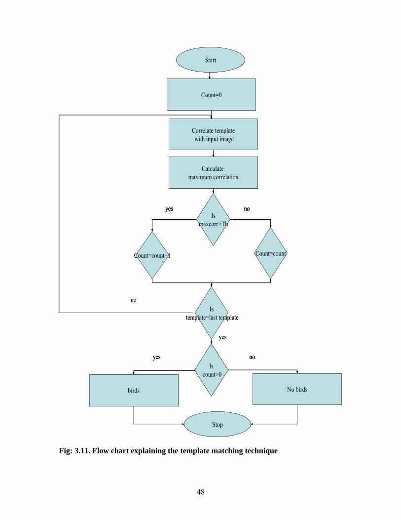
Start

Correlate templatewith input image

Ismaxcorr>Th

Count=count+1 Count=count

Calculate maximum correlation

Istemplate=last template

Iscount>0

Count=0

birds No birds

yes no

yes no

Stop

no

yes

Start

Correlate templatewith input image

Ismaxcorr>Th

Count=count+1 Count=count

Calculate maximum correlation

Istemplate=last template

Iscount>0

Count=0

birds No birds

yes no

yes no

Stop

no

yes

Fig: 3.11. Flow chart explaining the template matching technique

48

The software used to detect the web camera also stores images in the desired

format (jpeg in this study). Images have been taken by the web camera and stored in a

desired folder in a computer in regular intervals of time.

Steering DirectionBird Images

Control

Disperse Birds

Fig: 3.12. Block diagram for the control of autonomous boat

An image processing algorithm written using MATLAB® 6.5 acquires these input

images from the folder one by one and executes the algorithm. Output from the algorithm

is a simple number that gives the approximate location of birds. A basic stamp program

makes the autonomous boat turn in the desired direction. The cycle repeats every few

minutes.

49

CHAPTER 4: RESULTS AND DISCUSSION

Correct classification rate (CCR) and misclassification rate (MCR) were

calculated for image morphology algorithm. We manually observed the number of birds

in an input image and compared it with the number of objects recognized in the output

image of the algorithm. The other methods can be used to calculate the CCR on an entire

image. These methods however could not concentrate on each bird (object) in an image.

This might be because we trained and tested an entire image for CCR and MCR.

4.1 Image Morphology

Formulae used in this study are

Correct Classification Rate (CCR) = birds recognized/birds present

Misclassification Rate (MCR) = non-birds recognized/total objects recognized

CCR and MCR have different denominator values and hence their sum is not equal to

100%.

4.1.1 Pelicans

Image morphology on HSV images (Table 4.1) produced greater accuracies

(97.7% on medium clear images) than image morphology on gray level (93.3% CCR)

and RGB images (84.1% CCR) regardless of difficulty level of images and size

thresholding. Though the misclassification rate (up to 11.1%) was high when HSV

images were tested, this rate may not be statistically significant and therefore can be

neglected. Size threshold on medium clear and unclear images reduced the accuracies

drastically.

Lowest CCR on medium clear images was 28.8% using RGB color space and on

unclear images was 23.8% on both gray level and RGB images.

50

Table: 4.1. Results obtained by testing image morphology algorithm on all types of images

Species Classific

ation Size

threshold Difficulty

level Gray level

RGB HSV

Pelicans CCR Before size Type 1 93.2 84.1 95.5 Type 2 93.3 84.4 97.7 Type 3 57.1 57.1 57.1 After size Type 1 84.1 81.8 95.5 Type 2 31.1 28.8 88.9 Type 3 23.8 23.8 38 MCR Before size Type 1 6.8 5.1 10.6 Type 2 2.3 2.5 12 Type 3 8 8 7.6 After size Type 1 2.6 2.7 8.7 Type 2 0 0 11.1 Type 3 0 0 0

Egrets CCR Before size Type 1 100 100 100 Type 2 84.6 80.7 92.3 Type 3 90.0 90.0 90.0 After size Type 1 90.9 90.9 100.0 Type 2 84.6 73.0 92.3 Type 3 80.0 80.0 80.0 MCR Before size Type 1 6.8 8.3 15.3 Type 2 21.4 8.6 22.5 Type 3 18 25 36 After size Type 1 2.6 0.0 8.3 Type 2 15.3 9.5 22.5 Type 3 20.0 20.0 33.3

Cormorants CCR Before size Type 1 90.0 90.0 90.0 Type 2 95.5 95.4 90.9 Type 3 46.1 46.1 46.2 After size Type 1 75.0 70.0 85.0 Type 2 86.3 81.8 77.2 Type 3 38.4 38.4 23.1 MCR Before size Type 1 5.2 5.6 10.0 Type 2 19.2 19.2 23.1 Type 3 25.0 25.0 25.0 After size Type 1 6.2 6.6 10.5 Type 2 20.8 21.7 22.7 Type 3 28.5 22.2 40.0

51

One reason might be the presence of many birds in few images. Unrecognizing

some of them after size thresholding might have reduced the CCR drastically. This would

have resulted in reduced accuracies after size thresholding.

Image morphology on unclear images produced less accuracy rates irrespective on

size thresholding. This may be due to poor quality of input images. As mentioned

previously, birds in some unclear images were small in size and size thresholding further

reduced the CCR to as low as 23.8%.

4.1.2 Egrets

Image morphology on HSV images produced better or equal CCR (80% to

100%) on many images of egrets whether or not size thresholding had been implemented.

However, misclassification rate was as high as 36% on unclear HSV images, which

cannot be neglected. Image morphology using other color models (GRAY and RGB) also

produced MCR as high as 21.4 % (on gray level images) and 25% (on RGB images) on

medium clear and unclear images respectively. Misclassification rate of HSV unclear

images before size thresholding was double that of misclassification rate of gray level

images. Choice of color model depends on the type of applications because some

applications might tolerate misclassification rate where as some may not.

4.1.3 Cormorants

Cormorants are species of birds that are bluish black in color. These species

swim with most of their bodies in water and only neck outside the water. Recognition

became difficult in such images. Clear and medium clear images were clear and CCR as

high as 90% and 95.5% were obtained. However recognition became difficult with

unclear images using all color models. Image morphology, especially on HSV unclear

52

images resulted in low classification rates and high misclassification rates. For example,

image morphology on unclear HSV images followed by size thresholding resulted in a

CCR which was as low as 23.1%. MCR on HSV unclear images was 25% before size

thresholding and 40% after size thresholding. MCR was more than CCR in this case.

Hence, HSV color model is not a better choice for recognizing cormorants using image

morphology algorithm developed for the study. RGB and GRAY color models produced

almost same CCR and MCR and therefore any one of them can be chosen.

Most of the time unclear images had dark background which was similar to the

color of birds. Hence, the algorithm was unable to distinguish between background and

birds and resulted in very high misclassification rates. Local threshold values that were

fixed using few images could not work properly on all other images. From the results it

can be concluded that image morphology did not work as expected on unclear cormorant

images.

Overall HSV color model dominated RGB and GRAY models when image

morphology was implemented on white birds (pelicans and egrets). The HSV color

model can be used in cases where a small amount of misclassification can be tolerated for

its high correct classification. Even though the misclassification rate was greater when

using HSV color space, it was efficient in recognizing birds in some unclear images.

However all color models worked equally on all black birds (cormorants) except on

unclear images. None of the color models produced expected accuracy rates on unclear

cormorants. Size thresholding, which was expected to reduce noise and remove pixels of

other objects, affected the accuracy rates to a great extent. Image morphology on medium

clear pelican images resulted in a drastic decrease of CCR after size thresholding. This

53

may be due to the presence of birds of smaller size which were normally recognized but

removed after size thresholding.

4.2 Artificial Neural Networks

The CCR is the number of images correctly recognized divided by the total

number of images. The MCR is the number of images misclassified divided by the total

number of images. MCR is also (100-CCR) %. Figure 4.1 represents the results obtained

by testing the ANN algorithm. As indicated the first set of results in the graph represent

the results of testing pelicans and egret images and set 2 represents cormorants. The first

peak, second peak and the third peak in each set represents Type 1, Type 2 and Type 3

images respectively.

0

10

20

30

40

50

60

70

80

90

100

1 2

CC

R(%

)

Type 1Type 2Type 3

1 Pelicans/Egrets2 Cormorants

Fig: 4.1. Results from the ANN algorithm

54

We trained the ANN model to recognize pelicans and egrets using the same

algorithm. ANN models for every species would require the operation of a number of

algorithms simultaneously on the semi-autonomous boat. Taking into consideration, the

application point of view of all the algorithms in real time, we generalized the species of

birds to the maximum extent.

Table 4.2 includes all the results in a tabular form. While ANN worked very well on all

Type 1 images, CCR on Type 2 and Type 3 images reduced.

Table: 4.2. Tabulated results from ANN algorithm Bird Type of Image CCR (%) Pelicans and Egrets Type 1 100.0 Pelicans and Egrets Type 2 70.0 Pelicans and Egrets Type 3 67.7 Cormorants Type 1 100.0 Cormorants Type 2 62.5 Cormorants Type 3 57.1

Artificial neural network model produced almost equal CCR on Type 2 and Type

3 images. However, all types of images of pelicans, egrets and cormorants were

recognized with satisfactory CCR.

4.3 Template Matching We tested the images for the presence or absence of birds separately on each

section and each recognition method. The CCR is the number of images correctly

recognized divided by the total number of images. The MCR is the number of images

misclassified divided by the total number of images. MCR is (100-CCR) %. We used

same databases for testing white birds such as pelicans, egrets and white ducks and

different databases to test blackish tinge birds such as cormorants though the algorithm is

the same for all birds. Test images included lakes in order to fix precise

55

threshold/boundary between images of birds and other objects. Testing algorithm

included ten Type 1, Type 2 and Type 3 images using different combinations of rows

removed and databases. We used databases of 10, 20, 30, 50, and 70 while testing

pelicans and egrets and only 10, 20, and 30 databases while testing cormorants, due to the

scarcity of dependable cormorant images of adequate size. Similar images have been

discarded. Sky pixels contributed to misclassification and therefore we included this

variable as one of the factors affecting the CCR using template matching. In few images,

the first few rows in the input image had sky pixels. We tested the algorithm by removing

0, 50,100, and 150 rows from the input image. Irrespective of the number of rows

removed, each database had its own threshold value (E.g. 0.52 for database 50 and 0.5 for

database 70).

4.3.1 Pelicans and Egrets

Table 4.3 presents the accuracies obtained by testing several combinations of

rows removed and databases on all kinds of images of pelicans and egrets. However, for

better interpretation of results, graphs showing the correct classification rate (CCR) while

testing all Type 1, Type 2 and Type 3 images have been included in figures 4.2, 4.3, and

4.4 respectively.

Graphs indicated that removal of 150 rows regardless of database resulted in a

very poor performance (20% for database 10 and 20, 10% for database 30, and 40 and

50% for database 70) especially while testing Type 3 and Type 1 images. This may be

due to the presence of bird pixels in the first 150 rows of an image. Removal of bird

pixels would have resulted in misclassification.

56

Table: 4.3. Template matching results on pelicans and egrets

Database Rows Removed Type of Image Accuracy (%) 10 0 Type 1 80.0 Type 2 80.0 Type 3 70.0 10 50 Type 1 80.0 Type 2 70.0 Type 3 70.0 10 100 Type 1 90.0 Type 2 90.0 Type 3 60.0 10 150 Type 1 70.0 Type 2 80.0 Type 3 20.0 20 0 Type 1 90.0 Type 2 80.0 Type 3 60.0 20 50 Type 1 90.0 Type 2 60.0 Type 3 50.0 20 100 Type 1 90.0 Type 2 70.0 Type 3 80.0 20 150 Type 1 70.0 Type 2 60.0 Type 3 20.0 30 0 Type 1 80.0 Type 2 80.0 Type 3 70.0 30 50 Type 1 80.0 Type 2 80.0 Type 3 60.0 30 100 Type 1 90.0 Type 2 90.0 Type 3 60.0 30 150 Type 1 80.0 Type 2 90.0 Type 3 10.0

(Table continued)

57

50 0 Type 1 90.0 Type 2 80.0 Type 3 60.0 50 50 Type 1 90.0 Type 2 70.0 Type 3 50.0 50 100 Type 1 90.0 Type 2 80.0 Type 3 50.0 50 150 Type 1 57.1 Type 2 77.8 Type 3 10.0 70 0 Type 1 90.0 Type 2 80.0 Type 3 70.0 70 50 Type 1 80.0 Type 2 80.0 Type 3 60.0 70 100 Type 1 75.0 Type 2 66.7 Type 3 70.0 70 150 Type 1 71.4 Type 2 74.0 Type 3 50.0

Therefore, we discard the removal of 150 rows from the input images. As

mentioned previously, we used lake images for testing and fixing threshold i.e. the

boundary value between bird pixels and pixels of other objects. Table 4.3 and the graphs

obtained from testing all kinds of images depict database 10 as one of the good choices

for template matching especially on Type 3 images. However, most of the unclear images

including lakes crossed the threshold. This resulted in misclassification of lake images

and the algorithm produced positive result indicating the presence of birds even though

no bird was present. Removal of 0, 50 and 100 rows from Type 3 input images

encountered a similar problem with databases 20.

58

Type 1 Images

50

55

60

65

70

75

80

85

90

95

100

0 10 20 30 40 50 60 70 8Images in Database

CC

R(%

0

)

Rows removed 0Rows removed 50Rows removed 100Rows removed 150

Fig: 4.2. Results obtained while testing Type 1 images of pelicans and egrets

Type 2 Images

50

55

60

65

70

75

80

85

90

95

100

0 10 20 30 40 50 60 70 8Images in Database

CC

R(%

0

)

Rows removed 0Rows removed 50Rows removed 100Rows removed 150

Fig: 4.3. Results obtained while testing Type 2 images of pelicans and egrets

59

Most of the databases did not work properly on Type 3 images and databases

10 and 20 worked worst on them. However due to the problems associated with these

databases on Type 3 images, we consider database 10 and 20 ineffective for this study.

Figure 4.5 provides the various times taken by the algorithm for different combinations of

databases and the rows removed.

Databases 10, 20, and 30 took less than 40 seconds execution times. Database 70

took more than 85 seconds in all the tests. We cannot neglect the time taken by database

70. Therefore, we discarded database 70 from the study. However, we can consider the

time taken by database 50 (less than the time taken by database 75) as satisfactory.

Studying all the graphs and neglecting the removal of 150 rows from the input image, it

is evident that database 30 and 50 maintained consistency in CCR. However, database 50

maintained more consistency in the classification of Type 1 and Type 2 images.

Type 3 Images

0102030405060708090

100

0 10 20 30 40 50 60 70 8Images in Database

CC

R(%

0

)

Rows removed 0Rows removed 50Rows removed 100Rows removed 150

Fig: 4.4. Results obtained while testing Type 3 images of pelicans and egrets

60

Removal of no rows produced good CCR’s of 90%, 80% and 60% respectively on

Type 1, Type 2 and Type 3 images respectively using the database 50. Therefore, we

considered this as the best combination for template matching using the available images.

Best match might change with the type of images in the databases.

Overall study on pelicans and egrets resulted in poor classification of unclear

images. Though some databases (such as 10, 20) produced good CCR’s on unclear

images, all input images including lakes crossed threshold. However, the algorithm

worked well on all Type1 and Type 2 images. Table 4.4 includes the results of algorithm

after testing cormorants.

0102030405060708090

100110120130

0 50 100 150Rows Removed

Tim

e(Se

c)

Database 10Database 20Database 30Database 50Database 70

Fig: 4.5. Operation time for testing images using template matching

61

4.3.2 Cormorants

We tabulated all the CCR’s on all types of images of cormorants in table 4.4.

Table: 4.4. Template matching results on cormorants

Database Rows Removed Type of image CCR (%) 10 0 Type 1 90.0 Type 2 90.7 Type 3 10.0 10 50 Type 1 90.0 Type 2 91.7 Type 3 30.0 10 100 Type 1 100.0 Type 2 91.7 Type 3 40.0 10 150 Type 1 100.0 Type 2 81.8 Type 3 30.0 20 0 Type 1 80.0 Type 2 91.7 Type 3 60.0 20 50 Type 1 80.0 Type 2 91.7 Type 3 60.0 20 100 Type 1 80.0 Type 2 91.7 Type 3 80.0 20 150 Type 1 90.0 Type 2 90.9 Type 3 60.0 30 0 Type 1 80.0 Type 2 83.3 Type 3 60.0 30 50 Type 1 80.0 Type 2 83.3 Type 3 70.0 30 100 Type 1 80.0 Type 2 91.7 Type 3 80.0 30 150 Type 1 87.5 Type 2 90.9 Type 3 70.0

62

The same database for all birds would confuse the algorithm and might result in

classifying every object as a bird. Therefore, we tested cormorants separately using a

different database since they are of different color than pelicans and egrets. Adult

cormorants have black plumage and immature cormorants have brownish back and upper

wings. Figures 4.6 to 4.8 represent the results when we tested the algorithm on Type 1,

Type 2, and Type 3 images respectively.

Type 1 Images

70

75

80

85

90

95

100

0 10 20 30 4Images in Database

CC

R(%

0

)

Rows removed 0Rows removed 50Rows removed 100Rows removed 150

Fig: 4.6. Results obtained while testing Type 1 images of cormorants

The database is an important parameter and the results might differ when images

in a database change. Removal of 100 rows produced consistent CCR of 80%, 91.7% and

80% while testing Type 1, Type 2 and Type 3 images using database 20 compared to

90%, 90.9% and 60% when 150 rows were removed. We included the conclusions from

the implemented algorithms and recommendations for the future in the next chapter.

63

Type 2 Images

70

75

80

85

90

95

100

0 10 20 30 4Images in Database

CC

R(%

0

)

Rows removed 0Rows removed 50Rows removed 100Rows removed 150

Fig: 4.7. Results obtained while testing Type 2 images of cormorants

Type 3 Images

01020304050

60708090

100

0 10 20 30 4Images in Database

CC

R(%

0

)

Rows removed 0Rows removed 50Rows removed 100Rows removed 150

Fig: 4.8. Results obtained while testing Type 3 images of cormorants

64

CHAPTER 5: CONCLUSIONS AND RECOMMENDATIONS FOR THE FUTURE

The use of image processing techniques for the recognition of birds in

aquacultural ponds is a novel concept that enables increased flexibility in dispersing

predatory birds. Three image processing algorithms 1) image morphology, 2) artificial

neural networks, and 3) template matching were designed and tested. We extended the

algorithm to recognize birds in real time conditions. We developed necessary algorithms

for implementation. We used image processing and neural network tool boxes of

MATLAB® 6.5 version to develop algorithms. The training and testing of all the

algorithms were done on an Intel® Pentium® 4 CPU with a 3.0 GHz processor, 504 MB

of RAM, and a 150 GB hard drive. The size of most of the images used for the study was

640 by 480 (VGA) pixels. We considered this size taking into consideration the

implementation time and also the cost of digital cameras. Even the cheapest digital

camera could shoot images of that size. The image morphology algorithm took

approximately 15 seconds to produce results. The ANN model took three minutes to train

the images. However, results were obtained instantaneously (nearly one second) while

testing the images. Time taken by the template matching algorithm ranged from 16

seconds to 2 minutes based on the templates in a database and the number of rows of

horizon pixels removed from the input image. Template matching using a larger database

(for example a database with 70 templates) might not be recommended for real time

operation of autonomous boat to disperse birds from aquacultural stations.

Although some algorithms took more time to produce results, all the algorithms

produced encouraging results on all types of images on all species of birds (pelicans,

egrets, and cormorants) tested. Image morphology resulted in 57.1% to 97.7%, 73.0% to

65

100%, and 46.1% to 95.5% correct classification rates (CCR) respectively on images of

pelicans, cormorants and egrets before size thresholding. HSV color space produced

better results than the other two color models while testing the images of pelicans and

egrets using image the morphology algorithm. This algorithm worked well on images of

pelicans and egrets. However, it failed to produce accurate results with cormorant images

because most of the body (except the neck) is hidden under water. A limitation with this

algorithm is that the same threshold might not work properly under all lighting

conditions. Therefore a better algorithm that could change threshold values according to

lighting conditions might be developed in the future. The artificial neural network model

achieved 100% CCR while testing type 1 images and its classification success ranged

from 63.5% to 70.0%, and 57.1% to 67.7% while testing type 2, and type 3 images

respectively. The ANN model recognized all clear images, and produced satisfactory

results on other images. Accuracy can be improved by selecting proper images for

training. The template matching algorithm succeeded in classifying 90%, 80%, and 60%

of Type 1, Type 2, and Type 3 images of pelicans and egrets. This technique recognized

80%, 91.7%, and 80% of Type 1, Type 2, and Type 3 images of cormorants. Template

matching produced good results. Size and rotation of birds in an image might affect the

accuracy of the algorithm. Therefore a database that could represent different sizes and

angles of birds might further improve the accuracy of the algorithm.

All the algorithms can be used in the future in other applications such as the

detection of birds in fields, and the discrimination between weeds and plants. Clarity of

images generally increases with increasing size of images. Algorithms can be tested in

the future on faster computers. Algorithms might take less time to run on faster

66

computers. We tested only few species of predatory birds. However, this study can be

extended to other predatory birds such as herons, geese etc.

We considered the movement of birds in the study. However, movement of the

platform i.e. the autonomous boat could also be studied in the future. Infra red cameras or

cameras using other wavelengths can be used in the future for detecting birds. There is a

scope for future work on this thesis to further improve the performance of the image

processing algorithms. In this thesis we presented a basic neural network model to

classify the bird regions from the others. We can further improve this network accuracy

by training it on a larger data set. We developed individual algorithms for different

species of predatory birds. All the algorithms can be generalized and a single algorithm

for all species might be developed in the future. All the algorithms can be tested in real

time in the future. Also, there is a scope for the development of a more precise algorithm

to locate birds.

This work opened the door for other types of image processing and helped lay the

ground work for future work with bird or other species. Additionally, the consideration of

both moving targets and a moving platform increase the complexity of the task. Although

this work only touched on this marginally, future work should further explore each of

these challenges.

67

REFERENCES Aitkenhead, M. J., I. A. Dalgetty, C. E. Mullins, A. J. S. Mc. Donald, and N. J. C.

Strachan. 2003. Weed and Crop Discrimination Using Image Analysis and Artificial Intelligence Methods. Computers and Electronics in Agriculture, Vol 39, Pp157-171.

Anonymous. 2002. Website: Autonomous Vehicles

(http://www.csois.usu.edu/future/). Anonymous. 2003 .Website: Neural Network

(http://brain.web-us.com/brain/neural.html). Anonymous. 2004. Website: Cormorants

(http://www.bangornews.com/editorialnews/article.cfm?ID=436248). Bakircioglu, H. and E. Gelenbe. 1998. Random neural network recognition of

shaped objects in strong clutter. Proceedings of SPIE--the international society for optical engineering.Vol.33, No 07, Pp 22-28.

Barras, S. 2002.Online document: Bird Damage

(http://www.aphis.usda.gov/ws/researchreports/report2.pdf). Batra, S. W. T. 1988. Automatic Image Analysis for Rapid Identification of

Africanized Honey Bees In: Needham, G.R. (ed.), Africanized honeybees and bee mites. E. Horwood, Chichester, West Sussex, England, Pp 260-263.

Blackmore, S., H. Henrik, and F. Spyros. 2002. Specification of Behavioral

Requirements for an Autonomous Tractor. Proceedings of the July 26-27, 2002 ASAE Conference Chicago, Illinois, USA. Publication number 701P0502, Pp 13-23.

Bomford, M. and P.H .O. Brien. 1990. Sonic Deterrents in Animal Damage

Control: A Review of Device Test and Effectiveness. Wildlife Society Bulletin, Vol 18, Pp 411-422.

Bostelman, R. 2003. Online Document: NIST Autonomous Vehicles

(http://www.isd.mel.nist.gov/projects/iav/IAV.pdf). Bruder, J. A., V. N. Cavo, and M. C. Wicks. 1997. Bird Hazard Detection with Airport Surveillance Radar. Radar Conference. Publication number 449, Pp 160-163.

Bulanon, D. M., T. Kataoka, S. Zhang, Y. Ota, and T. Hiroma. 2001. Optimal Thresholding for the Automatic Recognition of Apple Fruits. American Society for Agricultural Engineers Publication No. 013133, Sacramento, California, USA.

68

Bulanon, D. M., T. Kataoka, Y. Ota, and T. Hiroma. 2002. A Segmentation Algorithm for the Automatic Recognition of Fuji Apples at Harvest. Biosystems Engineering, Vol 83, No 4, Pp 405-412.

Campbell, B. 1994. Introduction to Remote Sensing. New York, N.Y. The

Guilford Press, a Div. of Guilford Publication, Inc.

Casasent, D. P. 1992. Hierarchical Scene Analysis for Object Recognition. Proceedings of SPIE, Vol 1699, Pp 218-224.

Casasent, D., A. Talukder, P. Keagy, and T. Schatzki. 2001. Detection and Segmentation of Items in X-Ray Imagery. Transactions of the ASAE, Vol 44, No 2, Pp 337-345.

Chang, H. and U.Robles. 2000. Website: Template Matching (http://www-cs-

students.stanford.edu/~robles/ee368/matching.html). Creative, 2003. Website: Web Camera.

(http://www.creative.com/products/product.asp?prodid=628) Cruvinel, P. E. and E. R. Minate. 2002. Image Processing in Automated Pattern

Classification of Oranges. Presented as Paper number 701P0301 at the Proceedings of the World Congress of Computers in Agriculture and Natural Resources, Iguacu Falls, Brazil, March 2002, Pp 56-61.

Debipersad, S. C. and A. D. Broadhurst. 1997. Proceedings of the South African

Symposium on Communications and Signal Processing. Pp 33 – 36. El-Faki, M. S., N. Zhang, and D. E. Peterson. 2000. Weed Detection Using Color

Machine Vision. Transactions of the ASAE, Vol 43, No 6, Pp 1969-1978. Endangered Species Act. 1973. Online Document: Endangered Species Act

(http://ecos.fws.gov/tess_public/TESSWebpageVipListed?code=V&listings=0#B). Fadzil, M. H. A. and L. C. Choon. 1997. International Conference on Neural

Networks. IEEE Conference Proceedings .Vol 3, Pp 1638 – 1643. Glahn, J. F. and K. E. Brugger. 1995. The Impact of Double-Crested Cormorants

on the Mississippi Delta Catfish Industry. Colonial Water Birds, Vol 18, Pp 168-175.

Glahn, J. F., M. E .Tobin, and J. B. Harrell. 2000. Population Status and Management Issues in the Midwest: Possible Effects of Catfish Exploitation on Over Winter Body Condition of Double-Crested Cormorants. Symposium on Double-Drested Cormorants. United States Department of Agriculture, Animal and Plant Health Inspection Service Technical Bulletin, Vol 1879, Pp 107-113, Washington, D.C, USA.

69

Gliever, C. and D. C. Slaughter. 2001. Crop verses Weed Recognition with Artificial Neural Networks. Presented as Paper number 013104 at ASAE conference, Sacramento, California, August 2001.

Gonzalez, R. C. and R. E. Woods. 2003. Digital Image Processing second edition,

Pearson education (Singapore) Pte. Ltd, Delhi, India. Graves, R. E. 2004. A Primer on Robotic Milking. Presented as Paper number

044187 at ASAE conference, Ottawa, Ontario, Canada, August 2004. Griepentrog, H. W.

and H. Sogaard. 2003. Robotic Weeding in Sugar Beet.

Proceedings of the NJF’s 22nd Congress Nordic Agriculture in Global Perspective, Turku, Finland.

Grovum, M. A. and G. C .Zoerb. 1970. An Automatic Guidance System for

Autonomous Tractors. Presented as Paper number 011191, at ASAE conference, St.Joseph, Miami, USA.

Guyer, D. E, G. E. Miles, M. M. Schrieiber, O. R. Mitchell, and V. C. Vanderbitt

.1986. Machine Vision and Image Processing for plant identification. Transactions of the ASAE, Vol 29, No 6, Pp 1500-1507.

Hall, S. G., R. Price, and L. Wei. 2001. Design of an Autonomous Bird Predation

Reduction Device. Presented as Paper number 01-3131, at ASAE International Meeting, St. Joseph, MI.

Hall, S. G. and R. R. Price. 2003 a. An Autonomous Scare boat to Reduce Bird

Predation on Aquaculture Ponds. Louisiana Agriculture. Hall, S. G. and R. Price. 2003 b. Using Autonomous Robotic Vehicles for

Aquacultural and Environmental Applications. Presented as Paper number 03-202, at CSAE Annual Meeting, Montreal, Canada.

Hall, S. G. and R. R. Price. 2003 c. Mobile Semi-Autonomous Robotic Vehicles

Improve Aquacultural Ventures by Reducing Bird Predation and Improving Water Quality Monitoring. Abstract, Proceedings of the World Aquaculture Society, Louisville, KY.

Hall, S. G., R. R. Price, and N. Mandhani. 2004. Use of Autonomous Vehicles for Drinking Water Monitoring and Management in an Urban Environment. Presented as Paper number 047053, at ASAE/CSAE International Meeting, St. Joseph, MI.

Hall, S. G., N. Mandhani, A. Mudgundi, and R. R. Price. 2005. Autonomous

Vehicle Measurement and Analysis of Water Quality. Proceedings of the Institute of Biological Engineering, Pp. xx-xx.

70

Harvey, D. 2004. Website: Louisiana’s History (http://members.aol.com/DHarvey691/louisiana.html).

Hatem, I. and J. Tan. 2003. Cartilage and Bone Segmentation in Vertebra Images.

Transactions of the ASAE, Vol 46, No 5, Pp 1429-1434. Hemming, J. and T. Rath. 2001. Computer vision-based Weed Identification

under field Conditions using controlled Lighting. Journal of Agricultural engineering Research, Vol 78, No 3, Pp 223-243.

Hansen, G. L., E. M. Sparrow, J. Y. Kokate, K .J. Leland, and P. A. Iaizzo. 1997.

Wound Status Evaluation using Color Image Processing. IEEE Transactions on Medical Imaging, Vol 16, No 1, Pp 78-86.

Kondou, H. H., Y. Motonaga, H. Kitamura, K. Nakanishi, and T. Kameok. 2002.

Evaluation of Tree Vigor by Digital Camera Based on Fruit Color and Leaf Shape. Proceedings of the World Congress of Computers in Agriculture and Natural Resources 13-15, March 2002, Iguacu Falls, Brazil, ASAE Publication Number 701P0301, Pp 70-77.

Hatem, I. and J. Tan. 2003. Cartilage and Bone Segmentation in Vertebra Images. Transactions of the ASAE, Vol 46, No 5, Pp 1429-1434.

Hemming, J. and T. Rath. 2001. Computer vision-based Weed Identification under field Conditions using Controlled Lighting. Journal of Agricultural Engineering Research, Vol 78, No 3, Pp 223-243.

IrfanView. 2003. Website: IrfanView www.irfanview.com.

Jackway, P. T. 1995. Morphological Scale-Space with Application to Three-Dimensional Object Recognition. Unpublished Ph.D. Thesis. Queensland University of Technology, 204pp, 1995.

Jimenez, A. R., R. Ceres, and J. L. Pons. 2000. A Survey of Computer Vision Methods for Locating Fruit on Trees. Transactions of the ASAE, Vol 43, No 6, Pp 1911-1920.

Kapur, J. P. 1997. Website: Face Recognition (http://www.geocities.com/jaykapur/face.html).

Kavdir, I. and D. E. Guyer. 2002. Apple Sorting Using Artificial Neural Networks

and Spectral Imaging. Transactions of the ASAE, Vol 45, No 6, Pp 1995-2005. Kim, S. and T. Schatzki. 2001. Detection of Pinholes in Almonds through X-Ray

Imaging. Transactions of the ASAE, Vol 44, No 4, Pp 997-1003.

71

Kise, M., N. Nobura, I. Kasunobu, and T. Hideo. 2002. Enhancement of Turning Accuracy by Path Planning for Robot Tractor. Proceedings of the July 26-27, 2002 ASAE Conference Chicago, Illinois, USA. Publication number 701P0502, Pp 398-404.

Klein, A. L., M. Hovan, G. Genello, and P. Antonik. 2003. MMW Radar for

Dedicated Bird Detection at Airports and Air Fields. Online Document (http://www.int-birdstrike.com/Proceedingpdf%2026th/MMW%20RADAR%20FOR%20DEDICATED%20BIRD%20DETECTION%20AT%20AIRPORTS.pdf).

Lacey, G., S. Fergal, and W. Niall. 2004. Website: Global and Local Techniques.

(http://www.cs.tcd.ie/courses/computervision/ComputerVisionIntro2.html). Lauria, S. and R. J. Mitchell. 1998. Proceedings of the Neural Networks for

Signal Processing VIII. IEEE Signal Processing Society, Pp 539 – 546. Lee, C. H., S. H. Lee, and H. H. wang. 2001. Automatic Lean Tissue Generation

of Carcass Beef via Color Computer Vision. Presented as Paper number 016122 at ASAE conference, Sacramento, California, August 2001.

Leemans, V., H. Magein, and M. F. Destain. 1999. Defect Segmentation on

‘Jonagold’Apples using Color Vision and a Bayesian Classification Method. Computers and Electronics in Agriculture, Vol 23, Pp 43-53.

Lezoray, O., A. Elmoataz, and H. Cardot. 2003. A Color Object Recognition

Scheme: Application to Cellular Sorting. Machine vision and Applications, Vol 14, Pp 166-171.

Littauer, G. A., J. F .Glahn, D. S. Reinhold, and M. W. Brunson. 1997. Control of

Bird Predation at Aquaculture Facilities: Strategies and cost estimates. Southern Regional Aquaculture Center Publication No 402, Mississippi State Cooperative Extension Service, Mississippi State.

Liu, H. X. and B. Ram. 2001. Online Document: Vision –Based Stop Sign

Detection and Recognition System for Intelligent Vehicle (http://www.topslab.wisc.edu/resources/publications/ran/2001/ran_998.pdf).

Liu, J. and M. R. Paulsen. 2000. Corn Whiteness Measurement and Classification Using Machine Vision. Transactions of the ASAE, Vol.43, No 3, Pp 757-763.

MathWorks, 2005. Website: Image Processing Tool Box

(http://www.mathworks.com/applications/imageprocessing/).

Migratory Bird Treaty Act. 1918. Online document: Migratory Bird Treaty Act (http://migratorybirds.fws.gov/intrnltr/mbta/cnvntion.pdf).

72

Morimoto, E., M. Suguri, and M. Umeda. 2002. Online Document: Obstacle Avoidance System. (http://dspace.library.cornell.edu/retrieve/307/PM+01+009+Morimoto.pdf).

Nasrabadi, N. M. and W. Li. 1991. Object recognition by a Hopfield neural network. IEEE Transactions on Systems, Man and Cybernetics, Vol 21, No 6, Pp 1523 – 1535.

Neethirajan, S., C. Karunakaran, D. S. Jayas, and N. D. G. White. 2004. X ray

Image Analysis to Determine Air flow Path in Grain Bulks. Presented as Paper number 043080 at ASAE conference, Ottawa, Ontario, Canada, Aug 2004.

Nishiwaki, K., T. Togashi, K. Amaha, and K. Matsuo. 2001. Estimate Crop

Position Using Template Matching in Rice Production. Presented as Paper number 013103, at ASAE conference, Sacramento, California, August 2001.

Nishiwaki, K., T. Togashi, and K. Amaha. 2002. Vision-Based Speed and Yaw

Angle Measurement System. Proceedings of the July 26-27, 2002 ASAE Conference Chicago, Illinois, USA. Publication number 701P0502, Pp 212-220.

Price, A., G. Taylor, and L. Kleeman. 2000. Online Document: Fast, Robust

Color Vision for the Monash Humanoid (http://www.ecse.monash.edu.au/centres/irrc/LKPubs/humanoid.PDF).

Price, R. R. and S.G. Hall. 2001. Biorobotics and Autonomous Machinery in

Agricultural and Bioproduction Systems. Presented as paper number 013131 at ASAE conference, Sacramento, California, August 2001.

Price, R.R. and S.G. Hall. 2002. Development of an Autonomous Boat for Bird

Reduction on Aquaculture Ponds. Presented as Paper number 023110, at ASAE. Ruiz L.A., E. Molto, F. Juste, F. Pla, and R. Valiente. 1996. Location and

Characterization of the Stem-Calyx Area on Oranges by Computer Vision. Journal of Agricultural Engineering Research, Vol 64, Pp 165-172.

Seipelt, F., A. Bunger, R. Heeren, D. Kahler, M. Lullmann, and G. Pohl. 2003.

Computer Controlled Calf Rearing. Proceedings of the ASAE Conference, Fort Worth, Texas, USA, Publication number 701p0203, Pp 356-360.

Short, J. J., M. E. Kelley, R. J. Speelman, and R. E. McCarty. 1999. Bird Strike

Prevention: Applying Aero-Science and Bio-Science. Abstract Proceedings of the International Bird Strike Conference.

Shin, B. S., S. H. Kim, and J. U. Park. 2002. Autonomous Agricultural Vehicle

Using Overhead Guide. Proceedings of the ASAE Conference Chicago, Illinois, USA, Publication number 701P0502, Pp 261-269.

73

Simpson, A., T. Stombaugh, L. Wells, and J. Jacob. 2003. Imaging Techniques and Applications for UAV’s in Agriculture. Presented as Paper number 031105 at ASAE conference, Las Vegas, Nevada.

Sinha, D. and C. R. Giandina. 1990. Discrete Black and White Object

Recognition via Morphological Functions. IEEE Transactions on Pattern Analysis and Machine Intelligence Vol 12, No 3, Pp 275-293.

Soren , R. and C. Woodcock. 1996. Combining Spectral and Texture Data in the

Segmentation of Remotely Sensed Images. Photogrammetric Engineering and Remote Sensing. Journal of the American Society for Photogrammetry and Remote Sensing, Vol 62, No 2, Pp 181-194.

Stergiou, C. and S. Dimitrios. 1996. Website: Artificial Neural Network

Description (http://www.doc.ic.ac.uk/~nd/surprise_96/journal/vol4/cs11/report.html).

Stickley, A. R. and K. J. Andrews. 1989. Survey of Mississippi Catfish Farmers on Means, Effort, and Costs to Repel Fish-Eating Birds from Ponds. Proceedings of Eastern Wildlife Damage Control Conference Vol 4, Pp 105-108.

Sural, S., G. Qian, and S. Pramanik. 2002. Online Document: Segmentation and

Histogram Generation Using the HSV Color Space for Image Retrieval (http://www.cse.msu.edu/~pramanik/research/papers/2002Papers/icip.hsv.pdf), Pp 589-592.

Tao, Y., Z. Chen, H. Jing, and J. Walker. 2001. Internal Inspection of Deboned

Poultry Using X-Ray Imaging and Adaptive Thresholding. Transactions of the ASAE Vol 44, No 4, Pp 1005-1009.

Terawaki, M., T. Kataoka, H. Okamoto, and S. Hata. 2002. Distinction between

Sugar Beet and Weeds for Development of Automatic Thinner and Weeding Machine of Sugar Beet. Proceedings of the ASAE Conference Chicago, Illinois, USA. Publication number 701P0502, Pp 129-136.

Thiang., A. T. Guntoro, and R. Lim. 2001. Online Document: Type of Vehicle

Recognition Using Template Matching Method (http://faculty.petra.ac.id/thiang/download/paper/Pengenalan_Mobil_P017.pdf). Trnasport Canada. Airport Bird Detection System. Website: Bird Detection (http://www.tc.gc.ca/tdc/projects/air/e/5162.htm).

Wang, H. and D. Suter. 2003. Color Image Segmentation using Global Information and Local Homogenity. Proceedings of Seventh Digital Imaging Computing Techniques and Applications, Dec 10-12, 2003, Sydney.

Wu, Y. T. 1999. Website: Image Segmentation

(http://www.ablesw.com/3ddoctor/3dseg.html).

74

Xinwen, Y., Z. Shen, and S. Ninomiya. 2002. Online Document: Measuring

Geometrical Features of Insect specimens using Image Analysis (http://www.jsai.or.jp/afita/afita-conf/2002/part8/p591.pdf), Pp 591-595.

Young, S., C. H. Sibata, A. K. Ho, and K. H. Shin. 1996. IEEE International Conference on Acoustics, Speech, and Signal Processing, Vol 6, Pp 3418 – 3421.

Zhou, Z. H., Y. Jiang, Y. B. Yang, S. F. Chen. 2002. Online Document: ANN for Cancer Cell Detection. (http://cs.nju.edu.cn/people/zhouzh/zhouzh.files/publication/aim02.pdf).

75

APPENDIX A - IMAGE PROCESSING ALGORITHMS IMAGE MORPHOLOGY–PROGRAM 1 % Image morphology on pelicans and egrets % Clear all variables and figure windows close all; clear all; r =0; c =0; % Read input image and delete sky pixels a=imread('Birds 006.jpg'); %imwrite(a,'rgb.jpg','jpg'); figure(1),pixval(imshow(a),'on'); NP=60; % Size of window for local threshold is NP * NP No_rows=101; %-1 is the number of rows deleted S=size(a); for p=No_rows:S(1) r=r+1; c=0; for q=1:S(2) c=c+1; for k=1:3 I(r,c,k)=a(p,q,k); end end end figure(2),pixval(imshow(I)); I=double(I); s=size(I); % Add 200 rows and cols b=zeros(s(1)+200,s(2)+200); for i=101:s(1)+100 for j=101:s(2)+100 for k=1:3 b(i,j,k)=I(i-100,j-100,k); end end end b=uint8(b); figure(3),pixval(imshow(b));

76

%figure(2),pixval(imshow(a1),'on'); h1=rgb2hsv(b); figure(4),pixval(imshow(h1),'on'); %imwrite(h1,'hsv.jpg','jpg'); s1=size(h1); % Local threshold using HSV color space c=zeros(s1(1),s1(2)); for i=101:s1(1)-100 for j=101:s1(2)-100 if h1(i,j,1)<=0.7 && h1(i,j,2)<=0.08 && h1(i,j,3)>=.93 for p=i:i+NP for q=j:j+NP if (h1(p,q,1) <=.5 || h1(p,q,2) <=.5) && h1(p,q,3)>=.8 for m=1:3 c(p,q,m)=h1(p,q,m); end else for d=1:3 c(p,q,d)=0; end end end end end end end figure(5),pixval(imshow(c),'on'); s2=size(c); imwrite(c,'hsv.jpg','jpg'); c1=hsv2rgb(c); %figure(6),pixval(imshow(c1)); c1=rgb2gray(c1);

77

% Noise removal and size threshold bw = bwareaopen(c1,50); sb=size(bw); % Remove the added pixels I1=zeros(sb(1)-200,sb(2)-200); for i=101:sb(1)-100 for j=101:sb(2)-100 I1(i-100,j-100)=bw(i,j); end end %figure(7),pixval(imshow(I1),'on'); % Add null pixels in place of previously removed pixels of sky s3=size(I1); I2=zeros(s3(1)+100,s3(2)); for i=1:s3(1)+100 for j=1:s3(2) if i<=100 I3(i,j)=0; else I3(i,j)=I1(i-100,j); end end end I1=I3; % Define string functions to dilate i.e. set the border se90 = strel('line', 3, 90); se0 = strel('line', 3, 0); BWsdil = imdilate(I1, [se90 se0]); %figure(10), imshow(BWsdil), title('dilated gradient mask'); % Fill the holes BWdfill = imfill(BWsdil, 'holes'); figure(11), imshow(BWdfill); title('binary image with filled holes'); %imwrite(BWdfill,'C:\MATLAB6p5\work\Morphology\Outputs\afterholes.jpg','jpg');

78

% Calculate the number of objects in an image [labeled,numObjects] = bwlabel(BWdfill,4); numObjects I=BWdfill; % Divide image into 3 parts and locate birds s=size(I); sum_1=0; Img_1=zeros(s(1),s(2)/3); for i=1:s(1) for j=1:round(s(2)/3) Img_1(i,j)=I(i,j); if I(i,j)~=0 sum_1=sum_1+1; end end end sum_image(1)=sum_1; figure(11),pixval(imshow(I),'on'); figure(12),pixval(imshow(Img_1),'on'); sum_2=0; Img_2=zeros(s(1),s(2)/3); for i=1:s(1) for j=round(s(2)/3)+1:2*round(s(2)/3) Img_2(i,j-round(s(2)/3))=I(i,j); if I(i,j)~=0 sum_2=sum_2+1; end end end sum_image(2)=sum_2; figure(13),pixval(imshow(Img_2),'on'); sum_3=0; Img_3=zeros(s(1),s(2)/3); for i=1:s(1) for j=2*round(s(2)/3)+1:round(s(2)) Img_3(i,j-2*round(s(2)/3))=I(i,j); if I(i,j)~=0 sum_3=sum_3+1; end end end sum_image(3)=sum_3;

79

figure(14),pixval(imshow(Img_3),'on'); % Determine the location of bird based on the maximum number of pixels in an image max_image=max(sum_image); if max_image == sum_1 output=1 else if max_image==sum_2 output=2 else if max_image==sum_3 output=3 else output=4 end end end

IMAGE MORPHOLOGY–PROGRAM 2 % Image morphology on cormorants % Clear all variables and figure windows close all; clear all; r=0; c=0; % Read input image and delete sky pixels a=imread('cormorants_31.jpg'); %imwrite(a,'rgb.jpg','jpg'); figure(1),pixval(imshow(a),'on'); NP=60; % Size of window for local threshold is NP * NP No_rows=101; %-1 is the number of rows deleted S=size(a); for p=No_rows:S(1) r=r+1; c=0; for q=1:S(2) c=c+1; for k=1:3 I(r,c,k)=a(p,q,k); end end

80

end %figure(2),pixval(imshow(I)); a=double(I); s=size(a); % Add 200 rows and cols b=zeros(s(1)+200,s(2)+200); for i=101:s(1)+100 for j=101:s(2)+100 for k=1:3 b(i,j,k)=a(i-100,j-100,k); end end end b=uint8(b); figure(3),pixval(imshow(b)); %figure(2),pixval(imshow(a1),'on'); h1=rgb2hsv(b); figure(4),pixval(imshow(h1),'on'); %imwrite(h1,'hsv.jpg','jpg'); s1=size(h1); % Local threshold using HSV color space c=zeros(s1(1),s1(2)); for i=101:s1(1)-100 for j=101:s1(2)-100 if (h1(i,j,1)>=.67 && h1(i,j,1)<=0.7 && h1(i,j,3)<=0.2)||( h1(i,j,1)<=0.444 && h1(i,j,1)>0.3 && h1(i,j,3)<=0.23)||(h1(i,j,1)>=0.95 || h1(i,j,1)<=0.16 && h1(i,j,3)<=0.23) for p=i:i+NP for q=j:j+NP if (h1(p,q,1)>0.3 && h1(p,q,1) <=0.5 && h1(p,q,3)<=0.23) || (h1(p,q,1)>0.62 && h1(p,q,1)<0.7 && h1(p,q,3)<=0.23) ||(h1(p,q,1) >=.85 && h1(p,q,3)<=0.23) ||(h1(p,q,1)<0.15 && h1(p,q,3)<=0.23) for m=1:3 c(p,q,m)=h1(p,q,m); end else for d=1:3 c(p,q,d)=0; end end end end

81

end end end figure(5),pixval(imshow(c),'on'); s2=size(c); c1=hsv2rgb(c); % Write the color to grey converted image as jpeg figure(6),pixval(imshow(c1)); %imwrite(c1,'thresgrey.jpg','jpg'); c1=rgb2gray(c1); % Noise removal and size threshold bw = bwareaopen(c1,50); figure(7),pixval(imshow(bw),'on'); % figure(8), % subplot(1,2,1); imshow(c1); % subplot(1,2,2); imshow(bw); % Remove the added pixels sb=size(bw); I1=zeros(sb(1)-200,sb(2)-200); for i=101:sb(1)-100 for j=101:sb(2)-100 I1(i-100,j-100)=bw(i,j); end end figure(8),pixval(imshow(I1),'on'); % Add null pixels in place of previously removed pixels of sky s3=size(I1); I2=zeros(s3(1)+100,s3(2)); for i=1:s3(1)+100 for j=1:s3(2) if i<=100 I3(i,j)=0; else I3(i,j)=I1(i-100,j); end end end I1=I3;

82

% Define string functions to dilate i.e set the border se90 = strel('line', 3, 90); se0 = strel('line', 3, 0); BWsdil = imdilate(I1, [se90 se0]); figure(10), imshow(BWsdil), title('dilated gradient mask'); % Fill the holes BWdfill = imfill(BWsdil, 'holes'); figure(11), imshow(BWdfill); title('binary image with filled holes'); imwrite(BWdfill,'holes.jpg','jpg'); % Calculate the number of objects in an image [labeled,numObjects] = bwlabel(BWdfill,4); numObjects I=BWdfill; % Divide image into 3 parts and locate birds s=size(I); sum_1=0; Img_1=zeros(s(1),s(2)/3); for i=1:s(1) for j=1:round(s(2)/3) Img_1(i,j)=I(i,j); if I(i,j)~=0 sum_1=sum_1+1; end end end sum_image(1)=sum_1; figure(11),pixval(imshow(I),'on'); figure(12),pixval(imshow(Img_1),'on'); sum_2=0; Img_2=zeros(s(1),s(2)/3); for i=1:s(1) for j=round(s(2)/3)+1:2*round(s(2)/3) Img_2(i,j-round(s(2)/3))=I(i,j); if I(i,j)~=0 sum_2=sum_2+1; end

83

end end sum_image(2)=sum_2; figure(13),pixval(imshow(Img_2),'on'); sum_3=0; Img_3=zeros(s(1),s(2)/3); for i=1:s(1) for j=2*round(s(2)/3)+1:round(s(2)) Img_3(i,j-2*round(s(2)/3))=I(i,j); if I(i,j)~=0 sum_3=sum_3+1; end end end sum_image(3)=sum_3; figure(14),pixval(imshow(Img_3),'on'); % Determine the location of bird based on the maximum number of pixels in an image max_image=max(sum_image); if max_image == sum_1 output=1 else if max_image==sum_2 output=2 else if max_image==sum_3 output=3 else output=4 end end end ARTIFICIAL NEURAL NETWORK MODEL % Artificial neural network model to recognize all species % Clear workspace and close all matlab windows close all; clear all; clear img;

84

% Initilize all the variables epochs=1000; nbirds=4; % Number of bird images to be trained nnonbirds=3; % Number of non bird images to be trained ntotal=nbirds+nnonbirds; ninputs=13000; % Total inputs is No of rows * No of columns nHidden=5; % Number of hidden layers max_row=100; % Number of rows in the input image to be trained max_column=130; % Number of columns in the input image to be trained master=[]; Th=0.4; % Threshold value to seperate bird and non bird images % Read the images from directory and create a master matrix fext='.jpg'; uigetdir='C:\MATLAB6p5\work\NN\'; d=uigetdir; f=dir([d filesep '*' fext]); for y = 1 : (ntotal) fnam=f(y).name img{y}=imread(fnam,'jpg'); %img{y}=double(img{y}); u=0; for p=1:max_row for q=1:max_column u=u+1; master(u,y)=img{y}(p,q); end end end master=(0.9/255)*master; for x=1:ninputs for y=1:ntotal if master(x,y)==0 master(x,y)=0.1; end end end % Adjust the weight matrix so that the total weight is very less val=-0.03; for g=1:nHidden for h=1:ninputs W1(g,h)=val; val=val+.001;

85

if val==0 val=val+0.01 end if val>0.03 val=-0.03; end end end g=1; val=-0.03; for h=1:nHidden W2(g,h)=val; B1(h,g)=val; val=val+.001; if val>0.03 val=-0.03; end end B2=-0.01; % Training Phase % For bird nodules t=0.9 and for non-bird nodules t=0.1 error=0.5; i=1; eta=0.5; while ((i<epochs)&&(error>0.2)) i=i+1; i error for j=1:ntotal if j<=nbirds t=0.9; else t=0.1; end ip=master(:,j); o1 = logsig(W1 * ip + B1); o2 = logsig(W2 * o1 + B2); out2(j)=o2; errorval(j)=(t-o2);

86

error=max(errorval); delta2 = (dlogsig((W2 * o1 + B2),o2))*(t - o2); delta1 = zeros(nHidden, 1); for k = 1 : nHidden delta1(k) = dlogsig(((W1 * ip) + B1),o1(k)) * W2(k) * delta2; end W1 = W1 + eta * (delta1 * (ip)'); B1 = B1 + eta * delta1; W2 = W2 + eta * (delta2 * (o1)'); B2 = B2 + eta * delta2; end % Testing Phase y=[]; j1=0; out1=[]; correct_c = 0; correct_nc = 0; % For bird nodules for j=1:nbirds ip = master(:, j); t = 1; o1 = logsig(W1 * ip + B1); o2 = logsig(W2 * o1 + B2); out1(j)=o2; if o2 > Th op = 1; else op = 0; end o2 if t == op correct_c = correct_c + 1; end end % for non bird nodules for j=(nbirds)+1:(ntotal) ip = master(:, j); t = 0; o1 = logsig(W1 * ip + B1); o2 = logsig(W2 * o1 + B2); out1(j)=o2;

87

if o2 > Th op = 1; else op = 0; end o2 if t == op correct_nc = correct_nc + 1; end end acc = (correct_nc + correct_c) / ntotal; y = [y acc]; end % Accuracy Vs epochs plot plot(1 : epochs, y); legend('Accuracy'); xlabel('Epochs'); ylabel('Accuracy (in %)'); title('Accuracy (in %) versus Epochs'); TEMPLATE MATCHING MODEL % Clear all variables and figure windows close all; clear all; clear img; C=0; r=0; c=0; No_rows=151; %-1=No of rows removed % Read input image and delete sky pixels B = imread('C:\Documents and Settings\Uma Nadimpalli\Desktop\Temp\lake_8.jpg'); % Input image B=rgb2gray(B); %figure(1),imshow(B); S=size(B); for p=No_rows:S(1) r=r+1; c=0;

88

for q=1:S(2) c=c+1; I(r,c)=B(p,q); end end %figure(2),imshow(I); I=double(I); % Read all template images from the file and compute normal correlations fext='.jpg'; % Reads all the images in the directory with extension .jpg uigetdir='C:\MATLAB6p5\work\Temp Matching';

% Directory from which we read all templates d=uigetdir; f=dir([d filesep '*' fext]); sum=0; Average=0; count_60=0; count_65=0; count_70=0; count_75=0; count_80=0; count_85=0; count_90=0; count_95=0; l=1; for i=l:length(f) fnam=f(i).name; disp(sprintf('reading <%s>',fnam)); img{i}=imread(fnam,'jpg'); % Templates A=img{i}; A=rgb2gray(A); A=double(A); %Compute the cross-correlation of A and B C = normxcorr2(A,I); % xcorr2(A,B); %with normxcorr2,Normal correlation, if B is found exactly, then max(C(:)) == 1 corr(i)=max(C(:)); sum=sum+corr(i); if corr(i)>0.6 count_60=count_60+1; end

89

if corr(i)>0.65 count_65=count_65+1; end if corr(i)>0.7 count_70=count_70+1; end if corr(i)>0.75 count_75=count_75+1; end if corr(i)>0.8 count_80=count_80+1; end if corr(i)>0.85 count_85=count_85+1; end if corr(i)>0.9 count_90=count_90+1; end if corr(i)>0.95 count_95=count_95+1; end end Average=sum/length(f); AUTOMATION OF IMAGE MORPHOLOGY ALGORITHM % Clear all variables and figure windows close all; clear all; r=0; c=0; % Set input parameters and Read input image fext='.jpg'; uigetdir='C:\MATLAB6p5\work\Automation'; d=uigetdir; f=dir([d filesep '*' fext]);

90

pause_time=20; l=1; for No=l:1000 fnam{No}=f(No).name; a=imread(fnam{No}); a=double(a); % Remove sky pixels No_rows=101; %-1 is the number of rows deleted S=size(a); I2=zeros(S(1)-100,S(2)); for p=No_rows:S(1) r=r+1; c=0; for q=1:S(2) c=c+1; for k=1:3 I2(r,c,k)=a(p,q,k); end end end I2=uint8(I2); figure(2),pixval(imshow(I2)); I2=double(I2); s=size(I2); % Add 200 rows and cols b=zeros(s(1)+200,s(2)+200); for i=101:s(1)+100 for j=101:s(2)+100 for k=1:3 b(i,j,k)=I2(i-100,j-100,k); end end end b=uint8(b); figure(3),pixval(imshow(b)); %figure(2),pixval(imshow(a1),'on'); h1=rgb2hsv(b); %figure(4),pixval(imshow(h1),'on'); %imwrite(h1,'hsv.jpg','jpg'); s1=size(h1);

91

% Local threshold using HSV color space NP=60; % Local Window size is NP*NP c=zeros (s1(1),s1(2)); for i=101:s1(1)-100 for j=101:s1(2)-100 if h1(i,j,1)<=0.7 && h1(i,j,2)<=0.08 && h1(i,j,3)>=.93 for p=i:i+NP for q=j:j+NP if (h1(p,q,1) <=.5 || h1(p,q,2) <=.5) && h1(p,q,3)>=.8 for m=1:3 c(p,q,m)=h1(p,q,m); end else for d=1:3 c(p,q,d)=0; end end end end end end end figure(5),pixval(imshow(c),'on'); s2=size(c); %imwrite(c,'hsv.jpg','jpg'); c1=hsv2rgb(c); %figure(6),pixval(imshow(c1)); c1=rgb2gray(c1); %Noise removal and size thresholding bw = bwareaopen(c1,50); sb=size(bw); %Remove the added pixels I1=zeros(sb(1)-200,sb(2)-200); for i=101:sb(1)-100 for j=101:sb(2)-100 I1(i-100,j-100)=bw(i,j);

92

end end %figure(7),pixval(imshow(I1),'on'); % Add null pixels in place of previously removed pixels of sky s3=size(I1); I2=zeros(s3(1)+100,s3(2)); for i=1:s3(1)+100 for j=1:s3(2) if i<=100 I3(i,j)=0; else I3(i,j)=I1(i-100,j); end end end I1=I3; % Define string functions to dilate i.e. set the border se90 = strel('line', 3, 90); se0 = strel('line', 3, 0); BWsdil = imdilate(I1, [se90 se0]); %figure(10), imshow(BWsdil), title('dilated gradient mask'); % Fill the holes BWdfill = imfill(BWsdil, 'holes'); figure(11), imshow(BWdfill); title('binary image with filled holes'); %imwrite(BWdfill,'C:\MATLAB6p5\work\Morphology\Outputs\afterholes.jpg','jpg'); % Calculate the no of objects in an image [labeled,numObjects] = bwlabel(BWdfill,4); numObjects I=BWdfill; % Divide image into 3 parts and locate birds s=size (I); sum_1=0; Img_1=zeros(s(1),s(2)/3); for i=1:s(1)

93

for j=1:round(s(2)/3) Img_1(i,j)=I(i,j); if I(i,j)~=0 sum_1=sum_1+1; end end end sum_image(1)=sum_1; figure(11),pixval(imshow(I),'on'); figure(12),pixval(imshow(Img_1),'on'); sum_2=0; Img_2=zeros(s(1),s(2)/3); for i=1:s(1) for j=round(s(2)/3)+1:2*round(s(2)/3) Img_2(i,j-round(s(2)/3))=I(i,j); if I(i,j)~=0 sum_2=sum_2+1; end end end sum_image(2)=sum_2; figure(13),pixval(imshow(Img_2),'on'); sum_3=0; Img_3=zeros(s(1),s(2)/3); for i=1:s(1) for j=2*round(s(2)/3)+1:round(s(2)) Img_3(i,j-2*round(s(2)/3))=I(i,j); if I(i,j)~=0 sum_3=sum_3+1; end end end sum_image(3)=sum_3; figure(14),pixval(imshow(Img_3),'on'); % Determine the location of object based on maximum number of pixels in an image max_image=max(sum_image); if max_image == sum_1 output=1 else if max_image==sum_2 output=2 else if max_image==sum_3

94

output=3 else output=4 end end end % Clear variables pause(pause_time); I=0; clear a; clear b; clear c; clear I2; clear s; S=0; clear sum_1; clear sum_2; clear sum_3 sum_4; clear max_image output sum_image; r=0;c=0; clear fnam{No}; % End the program fext='.jpg'; uigetdir='C:\MATLAB6p5\work\Automation'; d=uigetdir; f=dir([d filesep '*' fext]); end

95

APPENDIX B – PAST RESEARCH ON OBJECT RECOGNITION

Year First Author Work Area Applications 2004 Neethirajan Image processing using X-

ray images Studied airflow paths in wheat samples

2003 Griepentrog Autonomous vehicles Weeding and Spraying 2003 Simpson Unmanned Aerial Vehicle precision agriculture 2003 Aitkenhead Neural network Discriminate plants and

weeds 2003,2002,2001 Price Autonomous vehicle and

machine vision Detect and disperse birds

2003,2002,2001 Hall Autonomous vehicle and machine vision

Detect and disperse birds

2003 Bostelman Autonomous vehicle and image processing using edge detection

Runs on road by tracking painted stripes

2003 Hatem Image processing using HSV color space

Cartilage and bone segmentation in vertebra images for grading beef

2002 Kise Autonomous tractor and image processing

Obstacle detection system

2002 Morimoto Autonomous vehicle and image processing using HSV color model

Runs on the road and detects the obstacles in the path

2002,2001 Nishiwaki Autonomous vehicle and vision system for template matching

Estimate plant positions

2002 Xinwen Image processing using gray level images

Measurement of geometric features of insects

2002 Kavdir Artificial neural networks Sorting of apples based on surface quality conditions

2002 Blackmore Autonomous vehicle mechanical weeding and field scouting

2001,1992 Casasent Image processing Extract nut meat from nuts

2001 Tao Image processing using X-ray imaging

detect the foreign objects in deboned meat

2001 Kim Image processing detect pinholes in almonds

2001 Bulanon Color segmentation using image processing

Recognize Fuji apples

2001 Liu Image processing using Vision based stop sign

96

HSV color model and neural networks

detection system

2001 Lee Image processing and artificial neural networks

Extraction of lean tissue from the carcass beef

2001 Gliever Artificial neural networks robotic weed control system

2001 Hemming Color image processing Weed identification 2001 Thiang Template matching Vehicle recognition 2000 Chang Template matching Face recognition 2000 Liu Image processing Measure the whiteness

of corn kernel 2000 El-Faki Neural networks

Color machine vision Detection of weeds in wheat and soybean fields

2000 Price Image processing using HSV color space

Robot

1999 Leemans Machine vision Defect segmentation on Jonagold apples

1998 Bakircioglu Artificial neural networks Automatic target detection

1998 Batra Image analysis Identification of Africanized honeybees

1997 Hansen Color image processing using HSV

Differentiation of wound severity

1996 Ruiz Image processing using color

Discriminate stemmed and de-stemmed oranges

1996 Soren Image texture Segmentation of test sites in an image

97

APPENDIX C – IMAGE PROCESSING TECHNIQUES FOR RECOGNITION OF BIRDS IN AQUACULTURAL

SETTINGS

Bird predation is one of the major concerns for fish culture in open ponds. A

novel method for dispersing birds is the use of autonomous vehicles. Image recognition

software can improve their efficiency. Several image processing techniques for

recognition of birds have been tested. A series of morphological operations were

implemented. We divided images into 3 types: Type 1, Type 2, and Type 3 based on the

level of difficulty of recognizing birds. These types were clear, medium clear and unclear

respectively. Local thresholding has been implemented using HSV (Hue, Saturation and

Value), GRAY and RGB (Red, Green and Blue) color models on all three sections of

images and results tabulated. Template matching using normal correlation and artificial

neural networks (ANN) are other methods that have been developed in this study besides

image morphology. Template matching produced satisfactory results irrespective of the

difficulty level of images but artificial neural networks (ANN) produced accuracies of

100%, 60% and 50% on Type 1, Type 2 and Type 3 images respectively. Correct

classification rate can be increased by further training of ANN model . Future research

will focus on testing the recognition algorithms in natural or aquacultural settings on

autonomous boats.

Keywords Image processing, Recognition, Morphology, Neural networks, Template

matching, Aquaculture.

Note: This manuscript was admitted for publication in Biotech progress in March

2005.

98

Ac.1 Introduction

Bird predation is one of the major concerns for fish culture in open ponds. Birds

such as pelicans, egrets, cormorants and herons arrive in flocks to consume abundant fish

in aquacultural ponds. Littauer et al. (1997) estimated that one egret can eat 1/3 pound of

fish per day, while a great heron can consume 2/3 pound of fish per day. Several methods

of controlling bird predation such as shooting and poisoning were ineffective or

unfriendly to the environment (Hall et al., 2001). Further, other birds such as Pelecanus

erythrorhynchos (American white pelican) and Pelecanus occidentalis (brown pelican)

are either endangered or protected species. They can be driven off from aquacultural

ponds but should not be killed (Migratory Bird Treaty Act, 1918 and Endangered Species

Act, 1973). A novel method for dispersing birds would be an autonomous boat that

recognizes the bird including location. The Biological and Agricultural Engineering

Department at the Louisiana State University developed a semi-autonomous boat for

chasing birds in the lake and measuring properties such as dissolved oxygen (DO),

biochemical oxygen demand (BOD) etc. Random motion worked well but chasing birds

was a challenge. Machine vision system on the semi-autonomous boat encountered

several problems. It worked well in the laboratory, but when taken outside, it faced

problems due to the brightness with intense sunlight. The machine vision system also had

problems due to the white color of birds. This necessitated more image processing

algorithms that would be suitable under all conditions.

Developing image-processing algorithms that work under all conditions could be

a better solution. These algorithms may also reduce unnecessary wandering of the boat in

the absence of birds, which saves solar power that the boat uses during cloudy or partly

99

sunny conditions. Three algorithms, namely image morphology, artificial neural

networks, and template matching have been developed and tested for this project. We

used the pictures taken by the semi-autonomous boat, some manually taken by our team

near the lakes and ponds, and some from the internet to test the efficacy of developed

algorithms.

Ac.2 Background and Literature Review

Object recognition is a broad area that can be implemented using several

techniques and image processing is one of those techniques. Several researchers have

used image-processing techniques in the past for object recognition. Image morphology is

an image processing technique commonly used for recognizing objects in a systematic

procedure. Several color models have been used in image morphology each having its

own advantages and limitations. The most frequently used color models in image

processing are GRAY, RGB, and HSV. Thresholding is an initial step in image

morphology and implementing it on gray scale image is the simplest and oldest of all

thresholding processes. Researchers who have worked on image morphology using gray

scale images are Casasent et al. (2001), Kim et al. (2001), Batra (1998) and Neethirajan

et al. (2004). Each pixel in a gray scale image is represented in terms of intensity.

Therefore, threshold value on such images can be fixed using only intensity.

Other color models commonly used are Red Green Blue (RGB) and Hue

Saturation Value (HSV). RGB has the advantage of fixing the threshold based on three

parameters namely Red, Green, and Blue. Bulanon et al. (2002) developed a

segmentation algorithm to segment Fuji apples based on red color difference between

objects in an image. Leemans et al. (1999), El-Faki et al. (2000) and Lezoray et al. (2003)

100

also worked on RGB images. Like gray level thresholding, color thresholding on RGB

images is also intensity variant.

Sural et al. (2002) found that RGB thresholding blurs the distinction between two

visually separable colors by changing brightness. HSV color space on the other hand can

determine the intensity and shade variations and retain pixel information. Hemming and

Rath (2001) worked on weed identification, Hatem et al. (2003) on cartilage and bone

identification, Price et al. (2000) on a robot known as Monash humoniod, and Lee et al.

(2001) on extraction of lean tissue from the carcass beef. Other morphological operations

follow thresholding for efficient removal of other pixels and retain bird pixels.

Besides image morphology, commonly used methods that gained wide range

popularity in many object recognition algorithms are ANN’s (artificial neural networks).

Aitkenhead et al. (2003) used a simple ANN to discriminate plants and weeds using plant

size as a parameter. Pre-processing the image resulted in removal of noise pixels, whose

presence would have slowed down the recognition process. Bakircioglu et al. (1998)

implemented automatic target detection using ANN’s to detect the targets in the presence

of clutter. Gliever et al. (2001) implemented a weed detection algorithm using a neural

network-based computational engine for a robotic weed control system to discriminate

cotton and weeds and achieved good accuracies.

Another method that has gained popularity in the recent years is object

recognition using template matching. Template matching is a method of

comparing/correlating an input image with a standard set of images known as templates.

Nishiwaki et al. (2001) used machine vision to recognize the crop positions using

template matching. Chang et al. (2000) developed template-matching algorithm in order

101

to match parts of the image corresponding to skin region and template face. Thiang et al.

(2001) have developed vehicle (car) recognition using camera as a sensor. Results

showed a good similarity level, of about 0.9 to 0.95 during daylight and 0.8 to 0.85 at

night.

Researchers concentrated mostly on accurate detection and differentiation of

several objects such as weeds, soil, plants, etc. from the background using several

techniques. No published research has been done on bird recognition followed by the use

of such recognition software to disperse birds from the lakes. The Biological and

Agricultural Engineering Department at the Louisiana State University Agricultural

Center developed a semi-autonomous boat for chasing birds in aquacultural stations

(Price, and Hall (2000, 2002), Hall and Price (2003 a, b, c), and Hall et al (2001, 2004,

2005)). One major advantage of this semi-autonomous boat is that the solar power saved

during the daytime can be used by boat in the absence of solar power. This allows the

boat to operate for weeks or months at a time. Other applications of semi-autonomous

boats include measuring water quality and locating the position of the boat (using Global

Positioning System) in lakes and ponds (Hall et al., 2005). They used a machine vision

system, designed by LEGO VISION COMMANDTM, to identify and chase birds.

Random motion worked well but chasing birds was a challenge. A novel method for

efficient chasing of birds is the development of different bird recognition methodologies

and using these algorithms on semi-autonomous boats to chase birds. Some among them

are image morphology, artificial neural networks (ANN) and template matching. Each

algorithm is explained in detail in the following section.

102

Ac.3 Implementation Methodology

Pictures of birds taken by a camera mounted on semi-autonomous boat (Price, and

Hall (2000, 2002), Hall and Price (2003 a, b, c), and Hall et al (2001, 2004, 2005)), some

obtained from the internet and some acquired locally were used in the study. Image-

processing and neural network toolboxes of MATLAB® 6p5 (Math Works, 2005) were

used for developing and testing all the algorithms. The three object recognition

algorithms developed for the study are

1. Image morphology

2. Artificial Neural Networks(ANN’s)

3. Template matching

For this paper, development of the relevant methodologies and preliminary

evaluation of these three methods were the objectives.

Ac.3.1 Image Morphology

The first among these methods is image morphology. This is a tool for extracting

useful information (or removing unnecessary information) from a picture in a step-by-

step procedure. The basic step in any image processing technique is thresholding that

removes extra and redundant information, also known as noise, from an image. Several

objects in an image contribute to noise. For instance, in an image containing birds such as

pelicans and egrets, the pixels containing the sky contributed to noise. These pixels are

called sky pixels. Most pixels containing the sky and birds (especially when the birds

were white such as egrets and pelicans) had the same intensity. A recognition algorithm

might misinterpret with the sky color as bird pixels. Removing all possible sky pixels

from picture is crucial. To do the operation, rows in an input image are cut to remove the

103

sky pixels. Other steps were also implemented in image morphology in detail in the

following algorithm.

1) Acquire an image.

2) Convert to required color space.

3) Remove sky pixels.

4) Add required rows and columns so that the last few pixels will have sufficient

neighbors for comparison.

5) Read pixels one by one.

6) Retain pixels whose value cross threshold 1.

7) Consider a window of required size (for e.g. 60 by 60) by taking pixel in step 6 as the

first pixel.

8) Within the window, retain only the pixels that cross threshold 2 and color other pixels

to black.

9) Convert the image to gray level and remove objects of smaller size, rows, and remove

extra rows and columns.

10) Continue the process until last pixel is scanned.

We implemented local thresholding as described on selected color spaces and

compared the performances of each color space. Local threshold that used two threshold

values has been chosen since a single threshold value might result in more noise pixels.

The other method implemented is Artificial Neural Networks (ANN’s).

Ac.3.2 Artificial Neural Networks

A feed forward back propagation neural network with 5 hidden layers was

designed. The number of elements in the input layer was from number of rows of the

104

input image multiplied by the number of columns. For each testing image output values

after log sigmoid function ranged from 0.1 to 0.9. A threshold value of 0.4 is fixed and

we consider the presence of birds if the output crosses threshold. The output layer is the

final layer and it indicates the presence/absence of birds in the tested image. Neural

networks learn through a training process and the success of artificial neural networks

depends on training.

Figure Ac.1 represents a general model of ANN. Signal at each layer is multiplied

by corresponding weights followed by the addition of bias at the end of each layer.

The value of in the figure can be represented as ka

k

n

iiji

n

j

m

kk bwkpa 1

111)*( += ∑∑∑

===

p

1

p2

p

3

p4

N11

N12

N13

N14

N21

N23

N22

N24

b13

b11

b12

b14

w111

w112

w113

w114

w141

w142

w143

w144

a1

a3

a2

a4

f11

f14

f13

f12

w211

w213

w214

w212

w2411

w242

w24 3

w24 4

b23

b22

b21

b24

f21

f24

f23

f22Log

sigmoid

∫ Output

Threshold

Fig: Ac.1. A generalized model of an artificial neural network

p1

p2

3

p4

N11

N12

N13

N14

N21

N23

N22

N24

b13

b11

b12

b14

w111

w112

w113

w114

w141

w142

w143

w144

a1

a3

a2

a4

f11

f14

f13

f12

w211

w213

w214

w212

w2411

w242

w24 3

w24 4

b23

b22

b21

b24

f21

f24

f23

f22Log

sigmoid

∫ Output

Threshold

p

105

In this training process, each input is multiplied by the corresponding weights

followed by the addition of bias after each layer. ANN’s output ranges from 0.1 to 0.9.

Error is calculated and propagated back. This entire process completes an epoch. Training

continues until error is less than 0.1 or number of epochs is greater than 1000. In the

testing phase signal passes threshold function and based on threshold the

presence/absence of birds in the input image is decided.

Another method implemented besides image morphology and ANN’s is template

matching.

Ac.3.3 Template Matching

Template matching is a method of comparing an input image with a standard set of

images known as templates. Templates are bird parts cut from various pictures. Normal

correlation between the input image and each template image is calculated. Correlation

according to Gonzalez et al. (2003) is

),(),(*1),(),(1

0

1

0nymxhnmf

MNyxhyxf

M

m

N

n++= ∑∑

−

=

−

=

o

Where and are two images of size ),( yxf ),( yxh NM × and is

the complex conjugate of .

*f

f

We illustrate a brief working of template matching in the figure 1.2. This

technique compares two images to decide if the desired shape (bird or bird part) is

present. We move the each template image from one pixel to other as shown in figure

Ac.2 and calculate (record) the maximum correlation/dot product between the template

and the input image.

106

1,1 1,2 1,3 1,4 1,n

2,1

3,1

m,1 m,2 m,3 m,4 m,n

4,1

2,n

3,n

4,n

Fig: Ac.2. The template matching technique

A threshold correlation value is fixed and if the maximum normal correlation

between input image and any template is above the threshold value, the input image has

bird(s). Accurate recognition of birds requires the use of a large number of template

images that could represent most angles and sizes of birds under different lighting

conditions as template matching is not invariant to rotation, size etc.

Ac.4 Results and Discussion

All images haven been divided into 3 types: a) Type 1, b) Type 2, and c) Type

3 based on the level of difficulty in recognizing birds. In Type 1 images, birds look like

the same as they look in-situ, i.e. non moving, clear and easily recognizable. A clear

1,1 1,2

1 2,2 2,q

1 ,2 q

p,1 p,2 p,q

2,

3, 3 3,

1,q

1,1 1,2 1,3 1,4 1,n

2,1

3,1

m,1 m,2 m,3 m,4 m,n

4,1

2,n

3,n

4,n

1,1 1,2

1 2,2 2,q

1 ,2 q

p,1 p,2 p,q

2,

3, 3 3,

1,q

107

distinction between birds and back ground was found. Type 2 images were not clear and

the distinction between birds and the background was less. Type 3 images were unclear

due to blurring of images, a poor quality camera, small size of birds, and movement of

camera while shooting birds.

Pictures of birds taken used in the study were obtained by a camera mounted on

the semi-autonomous boat (Price, and Hall (2000, 2002), Hall and Price (2003 a, b, c),

and Hall et al (2001, 2004, 2005)), some obtained from internet and some acquired

locally. Most images were 640 by 480 pixels in size. Images of smaller size were chosen

since an engineering compromise had to be made between the processing time of

algorithms and the clarity retention of input images. Aspect ratio of all the input images

was preserved. Testing was performed on an Intel centrino processor with 256 mega

bytes of ram.

Ac.4.1 Image Morphology

Input images were converted to gray level, red green and blue (RGB) and hue

saturation and value (HSV). For convenience sake, we refer them as gray level, RGB and

HSV images in this study.

Size threshold is the method of removing objects of smaller size and is capable of

reducing misclassification rate. Therefore, the performance of each color model before

and after size thresholding was tabulated. Image morphology algorithm has been tested to

calculate correct classification rate (CCR) and misclassification rate (MCR) on all types

of input images.

Correct Classification Rate (CCR) is birds recognized divided by birds present in

the image.

108

Misclassification Rate (MCR) is non-birds recognized divided by total objects

recognized in the image.

Table: Ac.1. Image morphology results

Classification

Size Threshold

Type of Image

Gray Level RGB HSV

CCR Before Size Threshold

Type 1 96.5 86.3 97.7

Type 2 93.7 85.4 97.9

Type 3 80.9 80.9 80.9

After Size Threshold

Type 1 86.3 84.0 97.7

Type 2 43.7 35.4 91.6

Type 3 47.6 47.6 62.0

MCR Before Size Threshold

Type 1 7.8 10.8 13.9

Type 2 9.5 5.8 4.5

Type 3 11.7 17.6 29.4

After Size Threshold

Type 1 2.6 2.7 6.9

Type 2 0.0 0.0 6.8

Type 3 20.0 20.0 30.7

Ac.4.1.1 Type 1 Images

Before size thresholding, image morphology on HSV images produced greater

CCR followed by gray level and RGB color models but both HSV and gray level images

produced almost the same CCR. After size threshold HSV images produced high CCR

compared to RGB and gray level images. The MCR was highest for HSV images and

109

gray level clear images produced the least MCR irrespective of whether size threshold

had been applied or not.

Ac.4.1.2 Type 2 Images

Image morphology on HSV and gray level images produced similar results. After

size threshold CCR of gray level and RGB images drastically dropped. However, the

CCR of HSV images remained the best among three at 97.9%. However, this was also

accompanied by a slight increase in MCR of HSV images that may not be statically

significant in this study.

Ac.4.1.3 Type 3 Images

Image morphology on Type 3 images resulted in equal CCR irrespective of color

spaces. However, after size threshold HSV images produced more CCR. HSV images

had higher MCR regardless of the application of size threshold.

Overall results from image morphology show that HSV images produced more

CCR compared to gray level and RGB images irrespective of the application of size

threshold. MCR was high for HSV images regardless of the application of size

thresholding. Size threshold reduced the MCR of all images except Type 3. Some of the

birds in Type 3 images were small in size (about 5 by 5 pixels). Size threshold in this

case would not have resulted in recognition of the birds. The HSV color model can be

used in cases where a small amount of misclassification can be tolerated with its high

CCR. Even though the misclassification rate was greater with the HSV color space, it was

efficient in recognizing birds in some unclear images. Figure Ac.3 represents input image

and image after size threshold using HSV color space.

110

a b

Fig: Ac.3. Image morphology on Type 3 images a) Sample input image b) image morphology on HSV image

dc

a b

Fig: Ac.4. Images after testing morphology algorithm on Type 3 images a) Sample input image b) Image morphology on gray level image c) Image morphology on RGB image d) Image morphology on HSV image

RGB and GRAY color models using the same algorithm resulted in images

without the presence of birds. In this case, birds were present but the algorithm on the

RGB and Gray level images could not recognize the birds. Even though the size of birds

111

was small, image morphology using HSV color space produced accurate results

compared to other color models. However, the misclassification rate was more for HSV

images as shown in the figure Ac.4.

Ac.4.2 Artificial Neural Networks

Input images of size 130 by 100 pixels were trained. Three types of images as

discussed previously were used to train ANN’s. Images once trained were not used for

testing ANN’s. Some images of lakes were also used in training and testing because

training requires inputs of bird images as well as non bird images. These lake images

were also divided into three types. ANN obtained accuracies of 100%, 60%, and 50% on

Type 1, Type 2, and Type 3 images respectively.

Type 1 images obtained high accuracies because these images were clear. Type 2

and Type 3 images obtained low accuracies because some images had birds, which were

small, and some images contained birds that were not clear due to the movement of

platform while using the camera. ANN’s may have been unable to make a clear-cut

distinction between images with and without birds due to the small size of birds. The

results presented on ANN’s were obtained by preliminary testing on a few images,

therefore accuracy can further be increased by proper selection of bird images for

training. In addition to training, clear images can assist the ANN in improving CCR.

Ac.4.3 Template Matching

Templates were stored in a database and accessed sequentially for correlating

each template image with input image. Three databases (30, 60 and 75) were used to

store template images. These were referred to as database 30, database 60 and database

112

75. Table Ac.2 represents accuracies with varying databases and rows of pixels above the

water horizon removed.

Table: Ac.2. Template matching results

S.No Database(No of images)

Rows of Sky Removed

Type of Image Accuracy (%)

1 30 100 Type 1 90.0

2 30 100 Type 2 90.0

3 30 100 Type 3 40.0

4 30 150 Type 1 90.0

5 30 150 Type 2 70.0

6 30 150 Type 3 50.0

7 60 100 Type 1 90.0

8 60 100 Type 2 80.0

9 60 100 Type 3 80.0

10 60 150 Type 1 100.0

11 60 150 Type 2 55.5

12 60 150 Type 3 80.0

13 75 100 Type 1 87.5

14 75 100 Type 2 66.7

15 75 100 Type 3 66.7

16 75 125 Type 1 100.0

17 75 125 Type 2 66.7

18 75 125 Type 3 70.0

These pixels contributed to misclassification and therefore were included as one

of the factors affecting the bird recognition classification rate using template matching.

113

The algorithm was tested by removing either the first 100 or the first 150 rows from the

input image.

Only 125 rows were removed instead of 150 from the input image when the

database was 75. This change was due to the presence of few template images in the

database that were bigger than the input image after deleting pixels above water horizon.

Correlation can be calculated only when the template image is smaller than the input

image.

Ac.4.3.1 Type 1 Images

As shown in the table 1.2, Template matching on Type 1 images produced good

accuracies, generally 90 to 100% irrespective of the databases and the number pixels

above the water horizon removed.

Ac.4.3.2 Type 2 Images

Template matching on Type 2 images produced good results when 100 sky pixel

rows were removed instead of 150. This may be due to the loss of some valuable

information when more rows were removed. In addition, medium clear images produced

good results with database 30. This may be due to the presence of objects other than

birds, which were similar to birds that correlated well with templates in other databases.

Ac.4.3.3 Type 3 Images

Accuracy of template matching on Type 3 images increased slightly with an

increase in the removal of sky pixels. Images in this case might include more sky pixels

and removal of 100 rows would not have been sufficient to remove certain objects, which

were not birds. Database 70 which was expected to produce better results compared to

114

data base 60 did not work as well as expected. This may be due to improper selection of

template images in database 70.

Database 60 and 100 rows of sky pixels removed has been considered best among

other combinations for the present study. This was because even though accuracies of this

algorithm on Type 1 and Type 2 images were slightly less compared to others, this

combination maintained its consistency in recognizing all kinds of images equally and

with a desired classification rate.

Ac.5 Conclusions

Different image processing techniques have been trained and tested to recognize

birds in an image efficiently. Image morphology using HSV color space worked well on

all types of images compared to other color spaces. ANN has worked better on Type 1

images than Type 2 and Type 3 images. Accuracies in these cases can be improved by

proper training of images. Template matching worked well and produced high accuracy

rates.

Ac.6 Future Recommendations

Our bird recognition algorithms have been tested on only two bird species,

pelicans and egrets. Other species such as cormorants and herons may be used in future

studies. Future research will also focus on testing the recognition algorithms in natural or

aquacultural settings on autonomous boats. Finally, the efficacy of using these algorithms

in guidance of the autonomous vehicle needs to be evaluated, especially with regards to

the speed of operation of each algorithm.

This paper has been approved as LSU AgCenter publication xxxx-05.

115

Ac.7 References

Aitkenhead, M. J., I. A. Dalgetty, C. E. Mullins, A. J. S. Mc. Donald, and N. J. C. Strachan. 2003. Weed and Crop Discrimination Using Image Analysis and Artificial Intelligence Methods. Computers and electronics in agriculture, Vol 39, Pp 157-171.

Anonymous. 2002. Website: Autonomous Vehicles

(http://www.csois.usu.edu/future/). Bakircioglu, H.and E. Gelenbe. 1998. Random Neural Network Recognition of

Shaped Objects in Strong Clutter. Proceedings of SPIE-The International Society for Optical Engineering, Vol 33, No 07, Pp 22-28.

Batra, S. W. T. 1988. Automatic Image Analysis for Rapid Identification of

Africanized Honey Bees In: Needham, G.R. (ed.), Africanized honey bees and bee mites. E. Horwood, Chichester, West Sussex, England, Pp 260-263.

Blackmore, S., H. Henrik, and F. Spyros. 2002. Specification of Behavioral

Requirements for an Autonomous Tractor. Proceedings of the ASAE Conference Chicago, Illinois, USA. Publication number 701P0502, Pp 13-23.

Bostelman, R. 2003. Online Document: NIST Autonomous Vehicles

(http://www.isd.mel.nist.gov/projects/iav/IAV.pdf).

Bulanon, D. M., T. Kataoka, Y. Ota, and T. Hiroma. 2001. A Segmentation Algorithm for the Automatic Recognition of Fuji Apples at Harvest. Biosystems Engineering, Vol 83, No 4, Pp 405-412.

Casasent, D., A. Talukder, P. Keagy, and T. Schatzki. 2001. Detection and

Segmentation of Items in X-Ray Imagery. Transactions of the ASAE, Vol 44, No 2, Pp 337-345.

Chang, H. and U. Robles. 2000. Website: Template Matching (http://www-cs-

students.stanford.edu/~robles/ee368/matching.html). El-Faki, M. S., N. Zhang, and D. E. Peterson. 2000. Weed Detection Using Color

Machine Vision. Transactions of the ASAE, Vol 43, No 6, Pp 1969-1978. Endangered Species Act. 1973. Online Document: Endangered Species Act

(http://ecos.fws.gov/tess_public/TESSWebpageVipListed?code=V&listings=0#B). Gonzalez, R. C. and R. E. Woods. 2003. Digital Image Processing second edition,

Pearson education (Singapore) Pte. Ltd, Delhi, India.

116

Gliever, C. and D. C. Slaughter. 2001. Crop verses Weed Recognition with Artificial Neural Networks. Presented as Paper number 013104 at ASAE conference, Sacramento, California.

Griepentrog, H. W.

and H. Sogaard. 2003. Robotic Weeding in Sugar Beet.

Proceedings of the NJF’s 22nd Congress Nordic Agriculture in Global Perspective, Turku, Finland.

Grovum, M. A. and G. C. Zoerb. 1970. An Automatic Guidance System for

Autonomous Tractors. Presented as Paper number 011191, at ASAE conference, St.Joseph, Miami, USA.

Hatem, I. and J. Tan. 2003. Cartilage and Bone Segmentation in Vertebra Images.

Transactions of the ASAE, Vol 46, No 5, Pp 1429-1434. Hall, S. G., R. Price, and L. Wei. 2001. Design of an Autonomous Bird Predation

Reduction Device. Presented as Paper number 01-3131, at ASAE International Meeting, St. Joseph, MI.

Hall, S. G. and R. R. Price. 2003 a. An Autonomous Scare boat to Reduce Bird

Predation on Aquaculture Ponds. Louisiana Agriculture. Hall, S. G. and R. Price. 2003 b. Using Autonomous Robotic Vehicles for

Aquacultural and Environmental Applications. Presented as Paper number 03-202, at CSAE Annual Meeting, Montreal, Canada.

Hall, S. G. and R. R. Price. 2003 c. Mobile Semi-Autonomous Robotic Vehicles

Improve Aquacultural Ventures by Reducing Bird Predation and Improving Water Quality Monitoring. Abstract, Proceedings of the World Aquaculture Society, Louisville, KY.

Hall, S. G., R. R. Price, and N. Mandhani. 2004. Use of Autonomous Vehicles

for Drinking Water Monitoring and Management in an Urban Environment. Presented as Paper number 047053, at ASAE/CSAE International Meeting, St. Joseph, MI.

Hall, S. G., N. Mandhani, A. Mudgundi, and R. R. Price. 2005. Autonomous

Vehicle Measurement and Analysis of Water Quality. Proceedings of the Institute of Biological Engineering, Pp. xx-xx.

Hemming, J. and T. Rath. 2001. Computer vision-based Weed Identification

under field Conditions using Controlled Lighting. Journal of Agricultural Engineering Research, Vol 78, No 3, Pp 223-243.

Kim, S. and T. Schatzki. 2001. Detection of Pinholes in Almonds through X-Ray

Imaging. Transactions of the ASAE, Vol 44, No 4, Pp 997-1003.

117

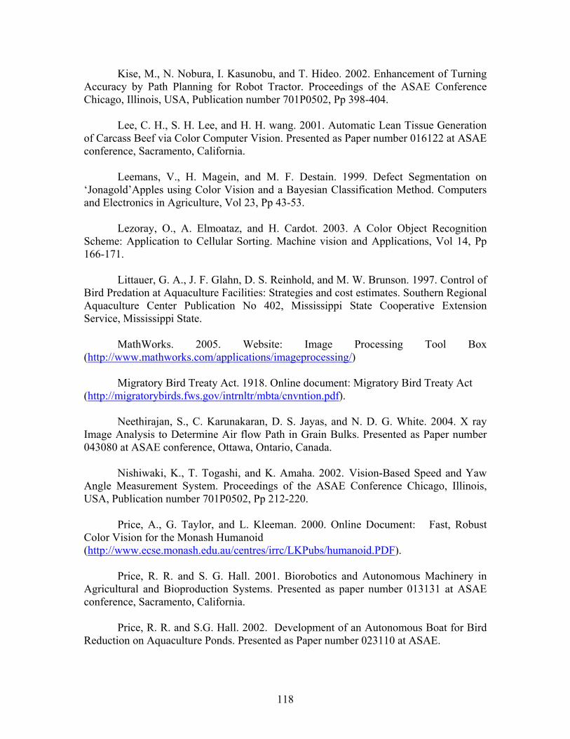
Kise, M., N. Nobura, I. Kasunobu, and T. Hideo. 2002. Enhancement of Turning Accuracy by Path Planning for Robot Tractor. Proceedings of the ASAE Conference Chicago, Illinois, USA, Publication number 701P0502, Pp 398-404.

Lee, C. H., S. H. Lee, and H. H. wang. 2001. Automatic Lean Tissue Generation

of Carcass Beef via Color Computer Vision. Presented as Paper number 016122 at ASAE conference, Sacramento, California.

Leemans, V., H. Magein, and M. F. Destain. 1999. Defect Segmentation on

‘Jonagold’Apples using Color Vision and a Bayesian Classification Method. Computers and Electronics in Agriculture, Vol 23, Pp 43-53.

Lezoray, O., A. Elmoataz, and H. Cardot. 2003. A Color Object Recognition

Scheme: Application to Cellular Sorting. Machine vision and Applications, Vol 14, Pp 166-171.

Littauer, G. A., J. F. Glahn, D. S. Reinhold, and M. W. Brunson. 1997. Control of

Bird Predation at Aquaculture Facilities: Strategies and cost estimates. Southern Regional Aquaculture Center Publication No 402, Mississippi State Cooperative Extension Service, Mississippi State.

MathWorks. 2005. Website: Image Processing Tool Box

(http://www.mathworks.com/applications/imageprocessing/) Migratory Bird Treaty Act. 1918. Online document: Migratory Bird Treaty Act

(http://migratorybirds.fws.gov/intrnltr/mbta/cnvntion.pdf).

Neethirajan, S., C. Karunakaran, D. S. Jayas, and N. D. G. White. 2004. X ray Image Analysis to Determine Air flow Path in Grain Bulks. Presented as Paper number 043080 at ASAE conference, Ottawa, Ontario, Canada.

Nishiwaki, K., T. Togashi, and K. Amaha. 2002. Vision-Based Speed and Yaw

Angle Measurement System. Proceedings of the ASAE Conference Chicago, Illinois, USA, Publication number 701P0502, Pp 212-220.

Price, A., G. Taylor, and L. Kleeman. 2000. Online Document: Fast, Robust

Color Vision for the Monash Humanoid (http://www.ecse.monash.edu.au/centres/irrc/LKPubs/humanoid.PDF).

Price, R. R. and S. G. Hall. 2001. Biorobotics and Autonomous Machinery in

Agricultural and Bioproduction Systems. Presented as paper number 013131 at ASAE conference, Sacramento, California.

Price, R. R. and S.G. Hall. 2002. Development of an Autonomous Boat for Bird

Reduction on Aquaculture Ponds. Presented as Paper number 023110 at ASAE.

118

Ruiz L. A., E. Molto, F. Juste, F. Pla, and R. Valiente. 1996. Location and Characterization of the Stem-Calyx Area on Oranges by Computer Vision. Journal of Agricultural Engineering Research, Vol 64, Pp 165-172.

Sural, S., G. Qian, and S. Pramanik. 2002. Online Document: Segmentation and

Histogram Generation Using the HSV Color Space for Image Retrieval (http://www.cse.msu.edu/~pramanik/research/papers/2002Papers/icip.hsv.pdf),

Pp 589-592. Tao, Y., Z. Chen, H. Jing, and J. Walker. 2001. Internal Inspection of Deboned

Poultry Using X-Ray Imaging and Adaptive Thresholding. Transactions of the ASAE Vol 44, No 4, Pp 1005-1009.

Thiang., A. T. Guntoro, and R. Lim. 2001. Online Document: Type of Vehicle

Recognition Using Template Matching Method (http://faculty.petra.ac.id/thiang/download/paper/Pengenalan_Mobil_P017.pdf).

Xinwen, Y., Z. Shen, and S. Ninomiya. 2002. Online Document: Measuring

Geometrical Features of Insect specimens using Image Analysis (http://www.jsai.or.jp/afita/afita-conf/2002/part8/p591.pdf), Pp 591-595.

119

VITA

Uma Nadimpalli was born on 25th December 1980 in Kakinada, India. She finished her

high school education in first class from Kakinada Public School, Kakinada, in 1996. She

joined the Andhra University College of Engineering in 1998 for a Bachelor of

Engineering degree in the Department of Electronics and Communication Engineering.

She graduated in first class with distinction in 2002. She joined Louisiana State

University in January 2003 for a master’s in biological and agricultural engineering. She

is currently working on “Image Processing Techniques to Identify Predatory Birds in

Aquacultural Settings” under the guidance of Dr. Randy Price and Dr. Steven Hall,

Associate Professors, Department of Biological and Agricultural Engineering, Louisiana

State University.

120