

Image Processing Cosimo Distante [email protected] Lecture 13: Motion.
98
-
Upload
pranav-haddon -
Category
Documents
-
view
268 -
download
0
Transcript of Image Processing Cosimo Distante [email protected] Lecture 13: Motion.

Last Time: Alignment
• Homographies• Rotational Panoramas• RANSAC• Global alignment• Warping• Blending

Today: Motion and Flow
• Motion estimation• Patch-based motion
(optic flow)• Regularization and line
processes• Parametric (global)
motion• Layered motion models

Why estimate visual motion?
• Visual Motion can be annoying– Camera instabilities, jitter– Measure it; remove it (stabilize)
• Visual Motion indicates dynamics in the scene– Moving objects, behavior– Track objects and analyze trajectories
• Visual Motion reveals spatial layout – Motion parallax
Szeliski

Classes of Techniques
• Feature-based methods– Extract visual features (corners, textured areas) and track them– Sparse motion fields, but possibly robust tracking– Suitable especially when image motion is large (10s of pixels)
• Direct-methods– Directly recover image motion from spatio-temporal image
brightness variations– Global motion parameters directly recovered without an
intermediate feature motion calculation– Dense motion fields, but more sensitive to appearance variations– Suitable for video and when image motion is small (< 10 pixels)
Szeliski

Patch-based motion estimation

Image motion
How do we determine correspondences?
Assume all change between frames is due to motion:
),(),( ),(),( yxyx vyuxIyxJ
I J

• Brightness Constancy Equation:),(),( ),(),( yxyx vyuxIyxJ
Or, equivalently, minimize :2)),(),((),( vyuxIyxJvuE
),(),(),(),(),(),( yxvyxIyxuyxIyxIyxJ yx
Linearizing (assuming small (u,v))using Taylor series expansion:
The Brightness Constraint
Szeliski

Gradient Constraint (or the Optical Flow Constraint)
2)(),( tyx IvIuIvuE Minimizing:
0)(
0)(
0
tyxy
tyxx
IvIuII
IvIuIIdv
E
du
E
In general 0, yx II
0 tyx IvIuIHence,
Szeliski

yx
tyx IvyxIuyxIvuE,
2),(),(),(
Minimizing
Assume a single velocity for all pixels within an image patch
ty
tx
yyx
yxx
II
II
v
u
III
III2
2
tT IIUII
LHS: sum of the 2x2 outer product of the gradient vector
Patch Translation [Lucas-Kanade]
Szeliski

Lavagna

Local Patch Analysis
• How certain are the motion estimates?
Szeliski


The Aperture Problem
TIIMLet
• Algorithm: At each pixel compute by solving
• M is singular if all gradient vectors point in the same direction• e.g., along an edge• of course, trivially singular if the summation is over a single pixel
or there is no texture• i.e., only normal flow is available (aperture problem)
• Corners and textured areas are OK
and
ty
tx
II
IIb
U bMU
Szeliski
Pollefeys

SSD Surface – Textured area

SSD Surface -- Edge

SSD – homogeneous area

Iterative Refinement
• Estimate velocity at each pixel using one iteration of Lucas and Kanade estimation
• Warp one image toward the other using the estimated flow field(easier said than done)
• Refine estimate by repeating the process
Szeliski

Optical Flow: Iterative Estimation
xx0
Initial guess:
Estimate:
estimate update
(using d for displacement here instead of u)
Szeliski

Optical Flow: Iterative Estimation
xx0
estimate update
Initial guess:
Estimate:
Szeliski

Optical Flow: Iterative Estimation
xx0
Initial guess:
Estimate:
Initial guess:
Estimate:
estimate update
Szeliski

Optical Flow: Iterative Estimation
xx0
Szeliski

Optical Flow: Iterative Estimation
• Some Implementation Issues:– Warping is not easy (ensure that errors in warping
are smaller than the estimate refinement)– Warp one image, take derivatives of the other so
you don’t need to re-compute the gradient after each iteration.
– Often useful to low-pass filter the images before motion estimation (for better derivative estimation, and linear approximations to image intensity)
Szeliski

Optical Flow: Aliasing
Temporal aliasing causes ambiguities in optical flow because images can have many pixels with the same intensity.
I.e., how do we know which ‘correspondence’ is correct?
nearest match is correct (no aliasing)
nearest match is incorrect (aliasing)
To overcome aliasing: coarse-to-fine estimation.
actual shift
estimated shift
Szeliski

Limits of the gradient method
Fails when intensity structure in window is poorFails when the displacement is large (typical
operating range is motion of 1 pixel)Linearization of brightness is suitable only for small
displacements• Also, brightness is not strictly constant in
imagesactually less problematic than it appears, since we
can pre-filter images to make them look similar
Szeliski

image Iimage J
aJwwarp refine
a
aΔ
+
Pyramid of image J Pyramid of image I
image Iimage J
Coarse-to-Fine Estimation
u=10 pixels
u=5 pixels
u=2.5 pixels
u=1.25 pixels
Szeliski

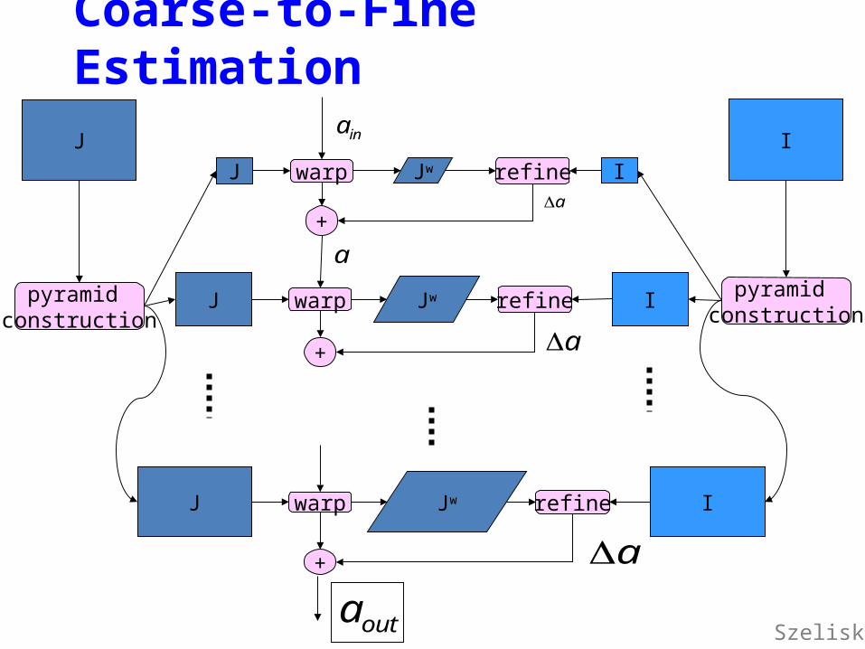
J Jw Iwarp refine
ina
a
+
J Jw Iwarp refine
a
a+
J
pyramid construction
J Jw Iwarp refine
a+
I
pyramid construction
outa
Coarse-to-Fine Estimation
Szeliski

Spatial Coherence
Assumption * Neighboring points in the scene typically belong to the same surface and hence typically have similar motions. * Since they also project to nearby points in the image, we expect spatial coherence in image flow.
Black

Formalize this Idea
Noisy 1D signal:
x
u
Noisy measurementsu(x)
Black

Regularization
Find the “best fitting” smoothed function v(x)
x
u
Noisy measurements u(x)
v(x)
Black

Membrane model
Find the “best fitting” smoothed function v(x)
x
uv(x)
Black

Membrane model
Find the “best fitting” smoothed function v(x)
x
uv(x)
Black

Membrane model
Find the “best fitting” smoothed function v(x)
uv(x)
Black

Spatial smoothness assumptionFaithful to the data
Regularization
x
uv(x)
Minimize:
1
1
2
1
2 ))()1(())()(()(N
x
N
x
xvxvxuxvvE
Black

Discontinuities
x
uv(x)
What about this discontinuity?What is happening here?What can we do?
Black

Robust EstimationNoise distributions are often non-Gaussian, having much heavier tails. Noise
samples from the tails are called outliers.• Sources of outliers (multiple motions):
– specularities / highlights– jpeg artifacts / interlacing / motion blur– multiple motions (occlusion boundaries, transparency)
velocity space
u1
u2
++
Black

Occlusion
occlusion disocclusion shear
Multiple motions within a finite region.
Black

Coherent Motion
Possibly Gaussian.
Black

Multiple Motions
Definitely not Gaussian.
Black

Weak membrane modelu
v(x)
1
1
2
1
2 ))(1())()1()(())()((),(N
x
N
x
xlxvxvxlxuxvlvE
x
}1,0{)( xl
Black

Analog line process
1
1
2
1
2 ))(())()1()(())()((),(N
x
N
x
xlxvxvxlxuxvlvE
1)(0 xl
Penalty function Family of quadratics
Black

Analog line process
1
1
2
1
2 ))(())()1()(())()((),(N
x
N
x
xlxvxvxlxuxvlvE
Infimum defines a robust error function.
1
12
1
2 )),()1(())()(()(N
x
N
x
xvxvxuxvvE
Minima are the same:
Black

Robust Regularization
x
uv(x)
Minimize:
1
12
11 )),()1(()),()(()(
N
x
N
x
xvxvxuxvvE
Treat large spatial derivatives as outliers.
Black

Robust EstimationProblem: Least-squares estimators penalize deviations between data & model with quadratic error fn (extremely sensitive to outliers)
error penalty function influence function
Redescending error functions (e.g., Geman-McClure) help to reduce the influence of outlying measurements.
error penalty function influence function
Black

Optical flow
Outlier with respect to neighbors.
)()()()(),( yxyxS vvuuvuE
Robust formulation of spatial coherence term
Black

• http://www.youtube.com/watch?v=V4r2HXGA8jw
• http://www.youtube.com/watch?v=ysGM3CfBVpU
• http://www.youtube.com/watch?feature=player_detailpage&v=U4taMDEozCs

Optimization
• Gradient descent• Coarse-to-fine (pyramid)• Deterministic annealing
Black

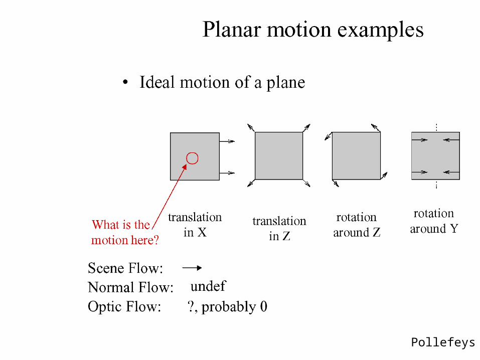
Parametric motion estimation

Global (parametric) motion models• 2D Models:• Affine• Quadratic• Planar projective transform (Homography)
• 3D Models:• Instantaneous camera motion models • Homography+epipole• Plane+Parallax
Szeliski

Motion models
Translation
2 unknowns
Affine
6 unknowns
Perspective
8 unknowns
3D rotation
3 unknowns
Szeliski

0)()( 654321 tyx IyaxaaIyaxaaI
• Substituting into the B.C. Equation:yaxaayxv
yaxaayxu
654
321
),(
),(
Each pixel provides 1 linear constraint in 6 global unknowns
0 tyx IvIuI
2 tyx IyaxaaIyaxaaIaErr )()()( 654321
Least Square Minimization (over all pixels):
Example: Affine Motion
Szeliski

Last lecture: Alignment / motion warping• “Alignment”: Assuming we know the correspondences,
how do we get the transformation?
),( ii yx ),( ii yx
2
1
43
21
t
t
y
x
mm
mm
y
x
i
i
i
i
• Expressed in terms of absolute coordinates of corresponding points…
• Generally presumed features separately detected in each frame
e.g., affine model in abs. coords…

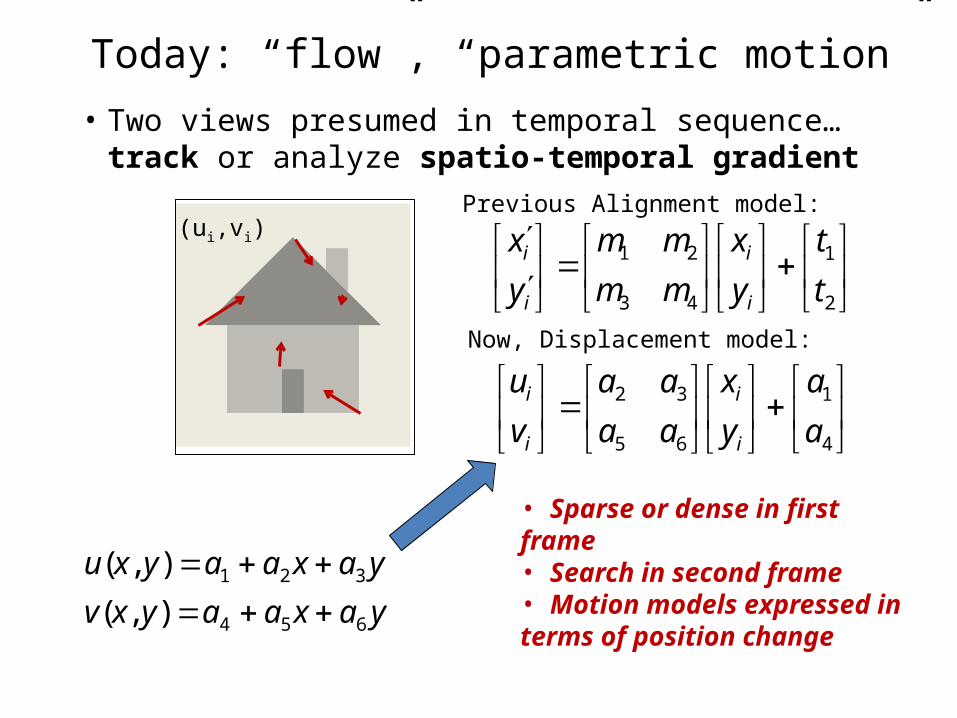
Today: “flow”, “parametric motion”• Two views presumed in temporal sequence…track or
analyze spatio-temporal gradient
),( ii yx),( ii yx
• Sparse or dense in first frame• Search in second frame• Motion models expressed in terms of position change

Today: “flow”, “parametric motion”• Two views presumed in temporal sequence…track or
analyze spatio-temporal gradient
),( ii yx),( ii yx
• Sparse or dense in first frame• Search in second frame• Motion models expressed in terms of position change

Today: “flow”, “parametric motion”• Two views presumed in temporal sequence…track or
analyze spatio-temporal gradient
),( ii yx),( ii yx
• Sparse or dense in first frame• Search in second frame• Motion models expressed in terms of position change

Today: “flow”, “parametric motion”• Two views presumed in temporal sequence…track or
analyze spatio-temporal gradient
),( ii yx
• Sparse or dense in first frame• Search in second frame• Motion models expressed in terms of position change
(ui,vi)

Today: “flow”, “parametric motion”• Two views presumed in temporal sequence…track or
analyze spatio-temporal gradient
• Sparse or dense in first frame• Search in second frame• Motion models expressed in terms of position change
(ui,vi)
Today: “flow”, “parametric motion”• Two views presumed in temporal sequence…track or
analyze spatio-temporal gradient
• Sparse or dense in first frame• Search in second frame• Motion models expressed in terms of position change
(ui,vi)
yaxaayxv
yaxaayxu
654
321
),(
),(
2
1
43
21
t
t
y
x
mm
mm
y
x
i
i
i
i
4
1
65
32
a
a
y
x
aa
aa
v
u
i
i
i
i
Previous Alignment model:
Now, Displacement model:

Quadratic – instantaneous approximation to planar motion 2
87654
82
7321
yqxyqyqxqqv
xyqxqyqxqqu
yyvxxu
yhxhh
yhxhhy
yhxhh
yhxhhx
','
and
'
'
987
654
987
321
Projective – exact planar motion
Other 2D Motion Models
Szeliski

Compositional AlgorithmLucas-Kanade
Baker-Mathews

ZxTTxxyyv
ZxTTyxxyu
ZYZYX
ZXZYX
)()1(
)()1(2
2
yyvxxu
thyhxh
thyhxhy
thyhxh
thyhxhx
',' :and
'
'
3987
1654
3987
1321
)(1
)(1
233
133
tytt
xyv
txtt
xxu
w
w
Local Parameter:
ZYXZYX TTT ,,,,,
),( yxZ
Instantaneous camera motion:
Global parameters:
Global parameters:
32191 ,,,,, ttthh
),( yx
Homography+Epipole
Local Parameter:
Residual Planar Parallax Motion
Global parameters:
321 ,, ttt
),( yxLocal Parameter:
3D Motion Models
Szeliski

• Consider image I translated by
• The discrete search method simply searches for the best estimate.
• The gradient method linearizes the intensity function and solves for the estimate
21
,00
2
,1
)),(),(),((
)),(),((),(
yxvvyuuxIyxI
vyuxIyxIvuE
yx
yx
00 ,vu
),(),(),(
),(),(
1001
0
yxyxIvyuxI
yxIyxI
Discrete Search vs. Gradient Based
Szeliski

Correlation and SSD
• For larger displacements, do template matching– Define a small area around a pixel as the template– Match the template against each pixel within a
search area in next image.– Use a match measure such as correlation,
normalized correlation, or sum-of-squares difference– Choose the maximum (or minimum) as the match– Sub-pixel estimate (Lucas-Kanade)
Szeliski

Shi-Tomasi feature tracker
1. Find good features (min eigenvalue of 22 Hessian)
2. Use Lucas-Kanade to track with pure translation
3. Use affine registration with first feature patch4. Terminate tracks whose dissimilarity gets too
large5. Start new tracks when needed
Szeliski

Tracking results
Szeliski

Tracking - dissimilarity
Szeliski

Tracking results
Szeliski

How well do thesetechniques work?

A Database and Evaluation Methodology for Optical Flow
Simon Baker, Daniel Scharstein, J.P Lewis, Stefan Roth, Michael Black, and Richard Szeliski
ICCV 2007http://vision.middlebury.edu/flow/

Limitations of Yosemite
• Only sequence used for quantitative evaluation
• Limitations:• Very simple and synthetic• Small, rigid motion• Minimal motion discontinuities/occlusions
Image 7 Image 8
Yose
mite
Ground-Truth FlowFlow Color
Coding
Szeliski

Limitations of Yosemite
• Only sequence used for quantitative evaluation
• Current challenges:• Non-rigid motion• Real sensor noise• Complex natural scenes• Motion discontinuities• Need more challenging and more realistic benchmarks
Image 7 Image 8
Yose
mite
Ground-Truth FlowFlow Color
Coding
Szeliski

Motion estimation 89
Realistic synthetic imagery• Randomly generate scenes with “trees” and “rocks”• Significant occlusions, motion, texture, and blur• Rendered using Mental Ray and “lens shader” plugin
Rock
Gro
ve
Szeliski

90
Modified stereo imagery
• Recrop and resample ground-truth stereo datasets to have appropriate motion for OF
Venu
sM
oebi
us
Szeliski

• Paint scene with textured fluorescent paint• Take 2 images: One in visible light, one in UV light• Move scene in very small steps using robot• Generate ground-truth by tracking the UV images
Dense flow with hidden texture
Setup
Visible
UV
Lights Image Cropped
Szeliski

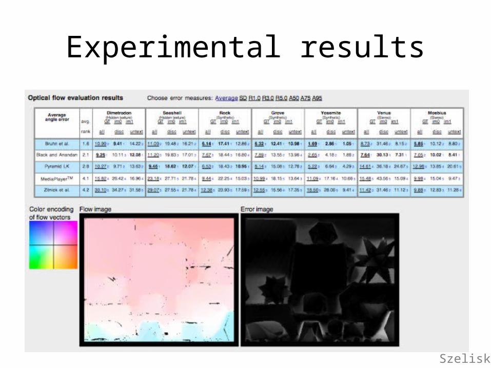
Experimental results
• Algorithms:• Pyramid LK: OpenCV-based implementation of
Lucas-Kanade on a Gaussian pyramid• Black and Anandan: Author’s implementation• Bruhn et al.: Our implementation• MediaPlayerTM: Code used for video frame-
rate upsampling in Microsoft MediaPlayer• Zitnick et al.: Author’s implementation
Szeliski
Motion estimation 93
Experimental results
Szeliski

Conclusions
• Difficulty: Data substantially more challenging than Yosemite
• Diversity: Substantial variation in difficulty across the various datasets
• Motion GT vs Interpolation: Best algorithms for one are not the best for the other
• Comparison with Stereo: Performance of existing flow algorithms appears weak
Szeliski

Layered Scene Representations

Motion representations
• How can we describe this scene?
Szeliski

Block-based motion prediction
• Break image up into square blocks• Estimate translation for each block• Use this to predict next frame, code difference
(MPEG-2)
Szeliski

Layered motion
• Break image sequence up into “layers”:
• =
• Describe each layer’s motion
Szeliski

Layered motion
• Advantages:• can represent occlusions / disocclusions• each layer’s motion can be smooth• video segmentation for semantic processing• Difficulties:• how do we determine the correct number?• how do we assign pixels?• how do we model the motion?
Szeliski

Layers for video summarization
Szeliski

Background modeling (MPEG-4)
• Convert masked images into a background sprite for layered video coding
• + + +
•=
Szeliski

What are layers?
• [Wang & Adelson, 1994; Darrell & Pentland 1991]
• intensities• alphas• velocities
Szeliski

Fragmented Occlusion
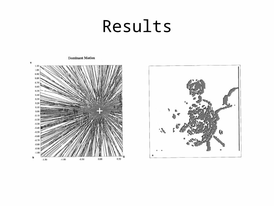
Results

Results

How do we form them?
Szeliski
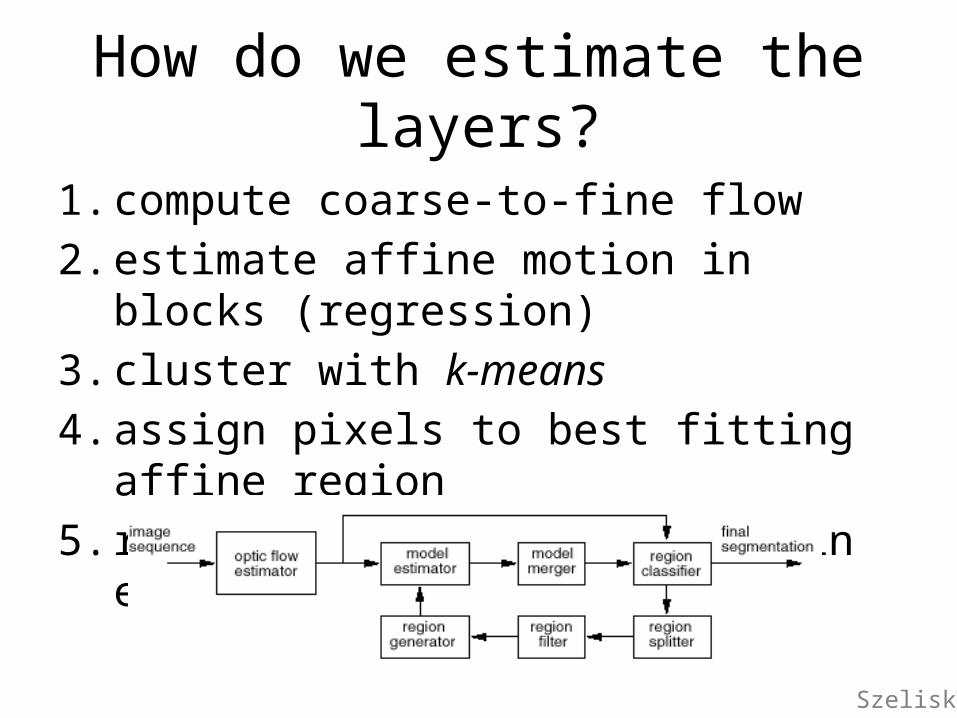
How do we estimate the layers?
1. compute coarse-to-fine flow2. estimate affine motion in blocks (regression)3. cluster with k-means4. assign pixels to best fitting affine region5. re-estimate affine motions in each region…
Szeliski

Layer synthesis
• For each layer:• stabilize the sequence with the affine motion• compute median value at each pixel• Determine occlusion relationships
Szeliski

Results
Szeliski
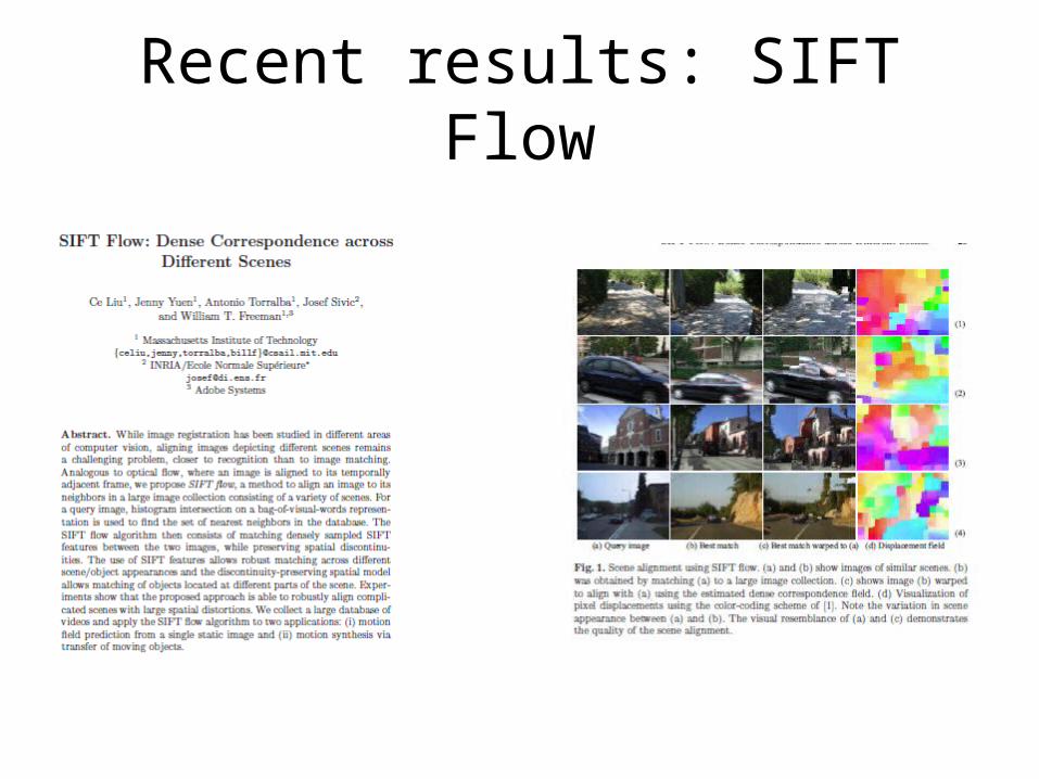
Recent results: SIFT Flow

Recent GPU Implementation
• http://gpu4vision.icg.tugraz.at/• Real time flow exploiting robust norm +
regularized mapping

Today: Motion and Flow
• Motion estimation• Patch-based motion (optic flow)• Regularization and line processes• Parametric (global) motion• Layered motion models

Project Ideas?
• Face annotation with online social networks?• Classifying sports or family events from photo
collections?• Optic flow to recognize gesture?• Finding indoor structures for scene context?• Shape models of human silhouettes? • Salesin: classify aesthetics?
– Would gist regression work?


