Image Formation - University of TorontoImage Formation Goal: Introduce basic concepts in image...

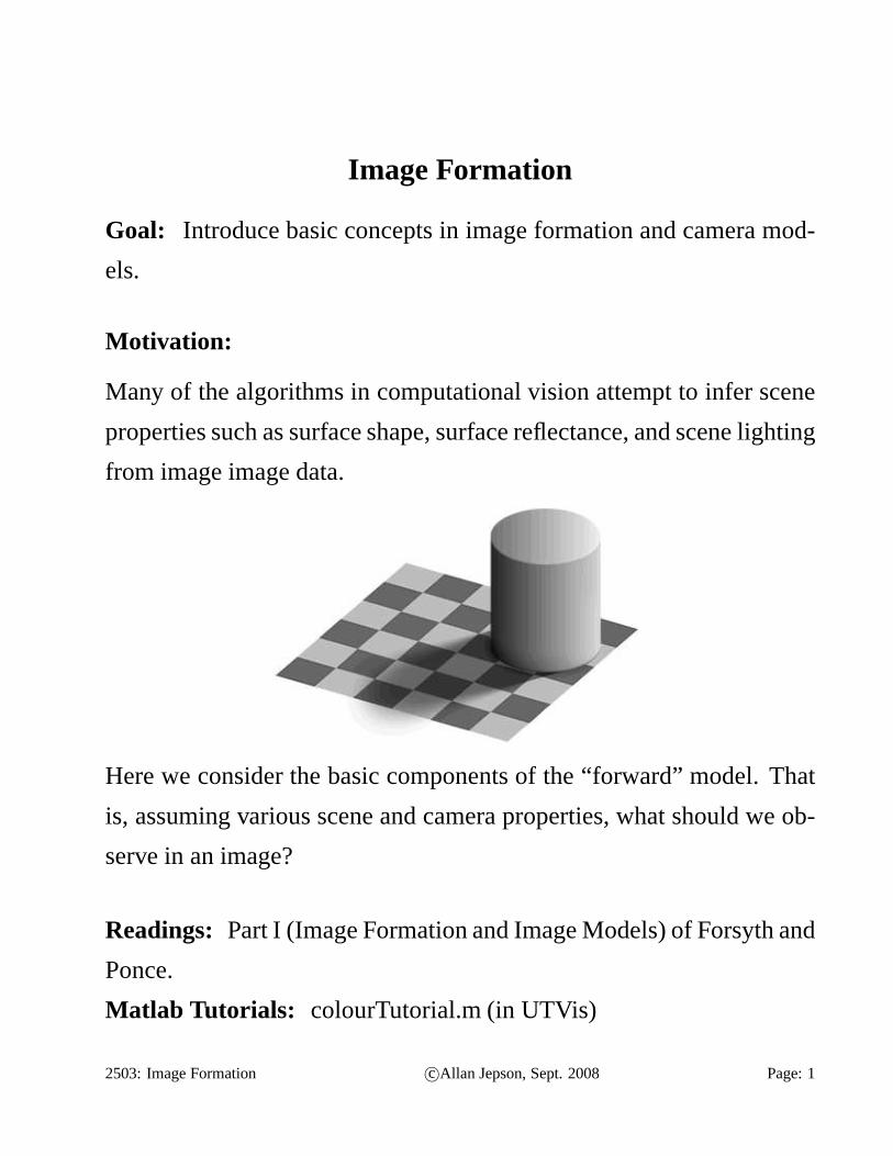
Image Formation

Goal: Introduce basic concepts in image formation and camera mod-

els.

Motivation:

Many of the algorithms in computational vision attempt to infer scene

properties such as surface shape, surface reflectance, and scene lighting

from image image data.

Here we consider the basic components of the “forward” model. That

is, assuming various scene and camera properties, what should we ob-

serve in an image?

Readings: Part I (Image Formation and Image Models) of Forsyth and

Ponce.

Matlab Tutorials: colourTutorial.m (in UTVis)

2503: Image Formation c©Allan Jepson, Sept. 2008 Page: 1

Thin Lens

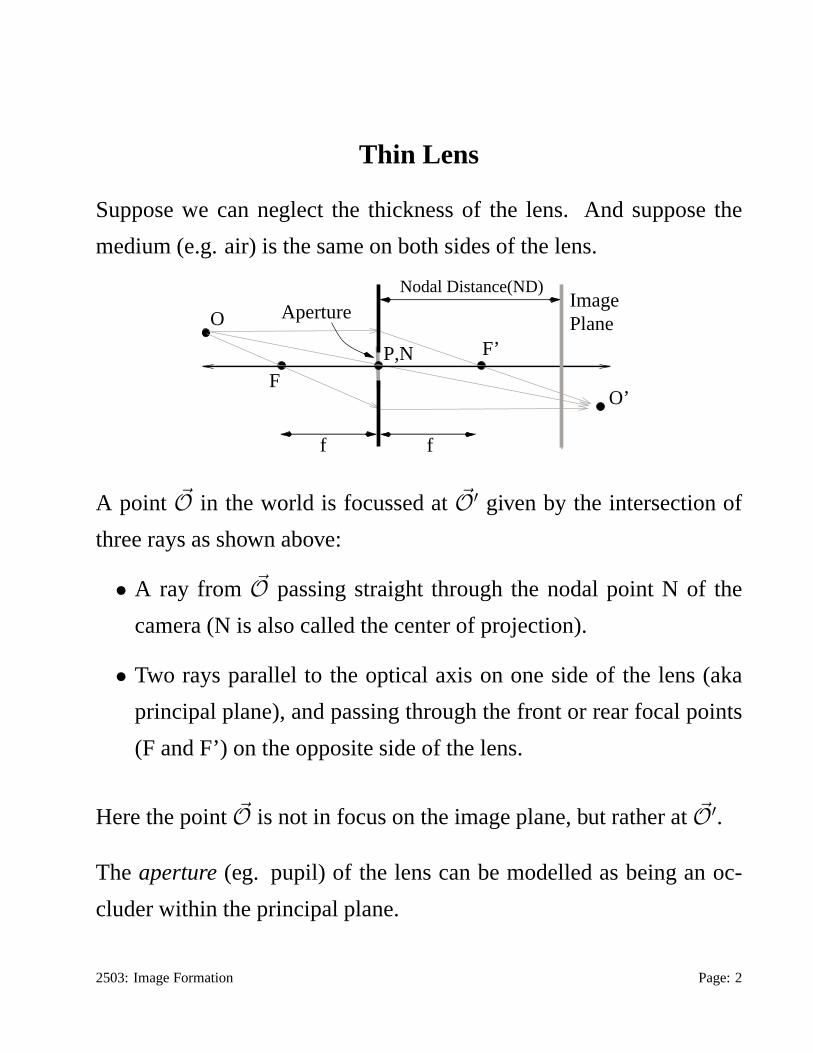
Suppose we can neglect the thickness of the lens. And supposethe

medium (e.g. air) is the same on both sides of the lens.

f

ImagePlaneO

f

FO’

F’

Nodal Distance(ND)

P,N

Aperture

A point ~O in the world is focussed at~O′ given by the intersection of

three rays as shown above:

• A ray from ~O passing straight through the nodal point N of the

camera (N is also called the center of projection).

• Two rays parallel to the optical axis on one side of the lens (aka

principal plane), and passing through the front or rear focal points

(F and F’) on the opposite side of the lens.

Here the point~O is not in focus on the image plane, but rather at~O′.

The aperture (eg. pupil) of the lens can be modelled as being an oc-

cluder within the principal plane.

2503: Image Formation Page: 2

General Lens Model

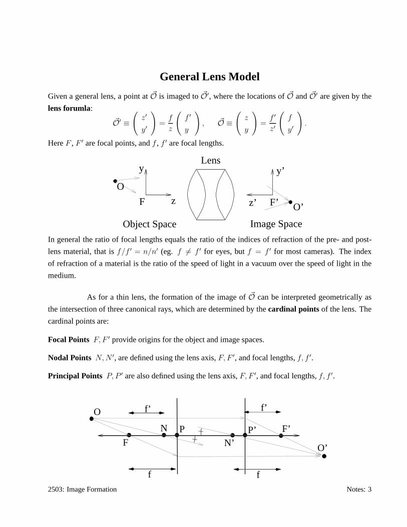
Given a general lens, a point at~O is imaged to~O′, where the locations of~O and ~O′ are given by the

lens forumla:

~O′ ≡

(

z′

y′

)

=f

z

(

f ′

y

)

, ~O ≡

(

z

y

)

=f ′

z′

(

f

y′

)

.

HereF , F ′ are focal points, andf , f ′ are focal lengths.

Lens

z z’

y’y

O

O’F’

Object Space Image Space

F

In general the ratio of focal lengths equals the ratio of the indices of refraction of the pre- and post-

lens material, that isf/f ′ = n/n′ (eg. f 6= f ′ for eyes, butf = f ′ for most cameras). The index

of refraction of a material is the ratio of the speed of light in a vacuum over the speed of light in the

medium.

As for a thin lens, the formation of the image of~O can be interpreted geometrically as

the intersection of three canonical rays, which are determined by thecardinal points of the lens. The

cardinal points are:

Focal Points F, F ′ provide origins for the object and image spaces.

Nodal Points N, N ′, are defined using the lens axis,F, F ′, and focal lengths,f, f ′.

Principal Points P, P ′ are also defined using the lens axis,F, F ′, and focal lengths,f, f ′.

O

O’

f’

ff

f’

F

F’P’N’

PN

2503: Image Formation Notes: 3

Lens Formula

An alternative coordinate system which is sometimes used towrite the lens formula is to place the

origins of the coordinates in the object and image space at the principal points P and P’, and flip both

the z-axes to be pointing away from the lens. These new z-coordinates are:

z = f − z,

z′ = f ′ − z′.

Solving forz andz′ and substituting into the previous lens formula, we obtain:

(f ′ − z) = ff ′/(f − z),

ff ′ = (f ′ − z′)(f − z)

z′z = z′f + zf ′

1 =f

z+

f ′

z′

The last line above is also known as the lens formula. As we have seen, it is equivalent to the one on

the previous page, only with a change in the definition of the coordinates.

For cameras with air both in front of and behind the lens, we have f = f’. This simplifies

the lens formula above. Moreover, the nodal and principal points coincide in both the object and scene

spaces (i.e.,N = P andN ′ = P ′ in the previous figure).

Finally it is worth noting that, in terms of image formation,the difference between this

general lens model and the thin lens approximation is only inthe displacement of the cardinal points

along the optical axis. That is, effectively, the change in the imaging geometry from a thin lens model

to the general lens model is simply the introduction of an absolute displacement in the image space

coordinates. For the purpose of modelling the image for a given scene, we can safely ignore this

displacement and use the thin lens model. When we talk about the center of projection of a camera in

a world coordinate frame, however, it should be understood we are talking about the location of the

nodal point N in the object space (and not N’ in the image space). Similarly, when we talk about the

nodal distance to the image plane, we mean the distance from N’ to the image plane.


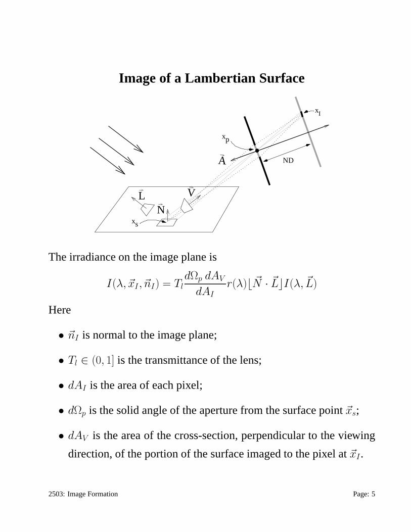
Image of a Lambertian Surface

N

xp

V

A

xs

xI

ND

L

The irradiance on the image plane is

I(λ, ~xI , ~nI) = TldΩp dAV

dAIr(λ)⌊ ~N · ~L⌋I(λ, ~L)

Here

• ~nI is normal to the image plane;

• Tl ∈ (0, 1] is the transmittance of the lens;

• dAI is the area of each pixel;

• dΩp is the solid angle of the aperture from the surface point~xs;

• dAV is the area of the cross-section, perpendicular to the viewing

direction, of the portion of the surface imaged to the pixel at ~xI.


Derivation of the Image of a Lambertian Surface

From our notes on Lambertian reflection, we have that the radiance (spectral density) of the surface is

R(λ, ~xs, ~V ) = r(λ)⌊ ~N · ~L⌋I(λ, ~L).

This is measured in Watts per unit wavelength, per unit cross-sectional area perpendicular to the

viewer, per unit steradian.

The total power (per unit wavelength) from the patchdAV , arriving on the aperature, is

P (λ) = R(λ, ~xs, ~V )dΩpdAV

A fractionTl of this is transmitted through the lens, and ends up on a pixelof areadAI . Therefore, the

pixel irradiance spectral density is

I(λ, ~xI , ~nI) = TlP (λ)/dAI ,

which is the expression on the previous page.

To simplify this, first compute the solid angle of the lens aperature, with respect to the

surface point~xs. Given the area of the aperature isdAp, we have

dΩp =|~V · ~A|dAp

||~xp − ~xs||2.

Here the numerator is the cross-sectional area of the aperature viewed from the direction~V . The

denominator scales this foreshortened patch back to the unit sphere to provide the desired measure of

solid angle. Secondly, we need the foreshortened surface areadAV which projects to the individual

pixel at ~xI having areadAI . These two patches are related by rays passing through the center of

projection~xp; they have the same solid angle with respect to~xp. As a result,

dAV = ||~xp − ~xs||2|~V · ~A|dAI

||~xp − ~xI ||2

The distance in the denominator here can be replaced by

||~xp − ~xI || = ND/|~V · ~A|.

Substituting these expression fordΩp, dAV , and||~xp −~xI || gives the equation for the image irradiance

due to a Lambertian surface on the following page.


Image of a Lambertian Surface (cont.)

This expression for the irradiance due to a Lambertian surface simpli-

fies to

I(λ, ~xI , ~nI) = TldAp

|ND|2| ~A · ~V |4 r(λ)⌊ ~N · ~L⌋I(λ, ~L)

Here,dAp is the area of the aperture.

Note the image irradiance:

• does not depend on the distance to the surface,||~xs − ~xp||;

• falls off like cos(θ)4 in the corners of the image. Hereθ is the

angle between the viewing direction~V and the camera’s axis~A.

Therefore, for wide angle images, there is a significant roll-off in

the image intensity towards the corners.

The fall off of the brightness in the corners of the image is called vi-

gnetting. The actual vignetting obtained depends on the internal struc-

ture of the lens, and will vary from the abovecos(θ)4 term.


Image Irradiance to Absorbed Energy

Spectral Sensitivity. The colour (or monochrome) pixel response is a

function of the energy absorbed by that pixel. For a steady image, not

changing in time, the absorbed energy at pixel~xI can be approximated

by

eµ(~xI) =

∫ ∞

0

Sµ(λ)CTAII(λ, ~xI , ~nI)dλ.

HereI(λ, ~xI , ~nI) is the image irradiance,Sµ(λ) is the spectral sensitiv-

ity of the µth colour sensor,AI is the area of the pixel, andCT is the

temporal integration time (eg. 1/(shutter speed)).

350 400 450 500 550 600 650 700 7500

0.2

0.4

0.6

0.8

1

Wavelength(nm)

Sen

sitiv

ity

Colour images are formed (typically) using three spectral sensitivities,

sayµ = R, G, B for the ‘red’, ‘green’ and ‘blue’ channel. The normal-

ized spectral sensitivities in the human retina are plottedabove.


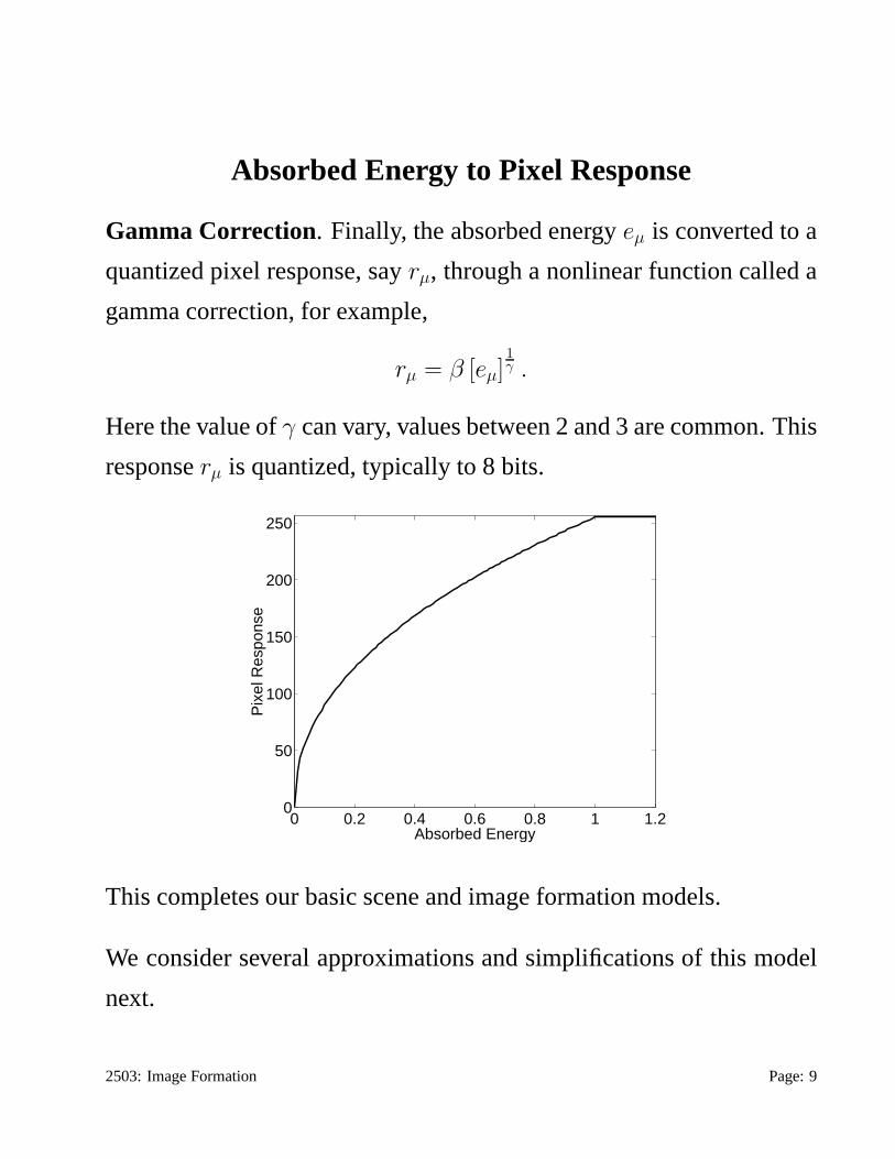
Absorbed Energy to Pixel Response

Gamma Correction. Finally, the absorbed energyeµ is converted to a

quantized pixel response, sayrµ, through a nonlinear function called a

gamma correction, for example,

rµ = β [eµ]1

γ .

Here the value ofγ can vary, values between 2 and 3 are common. This

responserµ is quantized, typically to 8 bits.

0 0.2 0.4 0.6 0.8 1 1.20

50

100

150

200

250

Absorbed Energy

Pix

el R

espo

nse

This completes our basic scene and image formation models.

We consider several approximations and simplifications of this model

next.


The Pinhole Camera

The image formation of both thick and thin lenses can be approximated

with a simple pinhole camera,

X

Z

Y

(X,Y,Z)(x,y,f)

N

y

x

Image Plane, Z=f

The image position for the 3D point(X, Y, Z) is given by the projective

transformation

x

y

f

=f

Z

X

Y

Z

By convention, the nodal distance|ND| is labelled asf (the “focal

length”). Note:

• for mathematical convenience we put the image plane in frontofthe nodal point (since this avoids the need to flip the image coordsabout the origin);

• image coordinatex is taken to the right, andy downwards. Thisagrees with the standard raster order.

• the primary approximation here is that all depths are taken to be infocus.


Orthographic Projection

Alternative projections onto an image plane are given by orthographic

projection and scaled orthographic projection.

(X,Y,Z)

Zx

Image Plane

X

y

Y

(X,Y,0)

Given a 3D point(X, Y, Z), the corresponding image location under

scaled orthographic projection is(

x

y

)

= s0

(

X

Y

)

Heres0 is a constant scale factor; orthographic projection usess0 = 1.

Scaled orthographic projection provides a linear approximation to per-

spective projection, which is applicable for a small objectfar from the

viewer and close to the optical axis.


Coordinate Frames

Consider the three coordinate frames:

• a world coordinate frame~Xw,

• a camera coordinate frame,~Xc,

• an image coordinate frame,~p.

The world and camera frames provide standard 3D orthogonal coordi-

nates. The image coordinates are written as a 3-vector,~p = (p1, p2, 1)T ,

with p1 andp2 the pixel coordinates of the image point.

Camera Coordinate Frame. The origin of the camera coordinates is

at the nodal point of the camera (say at~dw in world coords). Thez-axis

is taken to be the optical axis of the camera (with points in front of the

camera having a positivez value).

Next we express the transforms from world coordinates to camera co-

ordinates and then to image coordinates.


External Calibration Matrix

The external calibration parameters specify the transformation from

world to camera coordinates.

This has the form of a standard 3D coordinate transformation,

~Xc = Mex[ ~XTw , 1]T , (1)

with Mex a 3 × 4 matrix of the form

Mex =(

R −R~dw

)

. (2)

HereR is a 3 × 3 rotation matrix and~dw is the location of the nodal

point for the camera in world coordinates.

The inverse of this mapping is simply

~Xw = RT ~Xc + ~dw. (3)

In terms of the camera coordinate frame, the perspective transformation

of the 3D point~Xc (in the camera’s coordinates) to the image plane is

~xc =f

X3,c

~Xc =

x1,c

x2,c

f

. (4)

Heref is the nodal distance for the camera.


Internal Calibration Matrix

The internal calibration matrix transforms the 3D image position ~xc to

pixel coordinates,

~p = Min~xc, (5)

whereMin is a3 × 3 matrix.

For example, a camera with rectangular pixels of size1/sx by 1/sy,

with focal lengthf , and piercing point(ox, oy) (i.e., the intersection of

the optical axis with the image plane provided in pixel coordinates) has

the internal calibration matrix

Min =

sx 0 ox/f

0 sy oy/f

0 0 1/f

. (6)

Note that, for a 3D point~xc on the image plane, the third coordinate of

the pixel coordinate vector~p is p3 = 1. As we see next, this redundancy

is useful.

Equations (1), (4) and (5) define the transformation from~Xw, the world

coordinates of a 3D point to~p, the pixel coordinates of the image of

that point. The transformation is nonlinear, due to the scaling by X3,c

in equation (4).


Homogeneous Coordinates

It is useful to express this transformation in terms of homogeneous co-

ordinates,

~X hw = a( ~X T

w , 1)T ,

~p h = b~p = b(p1, p2, 1)T ,

for arbitrary nonzero constantsa, b. The last coordinate of these homo-

geneous vectors provide the scale factors. It is therefore easy to con-

vert back and forth between the homogeneous forms and the standard

forms.

The mapping from world to pixel coordinates can then be written as the

linear transformation,

~p h = MinMex~X h

w . (7)

Essentially, the division operation in perspective projection is now im-

plicit in the homogeneous vector~p h. It is simply postponed until~p h is

rescaled by its third coordinate to form the pixel coordinate vector~p.

Due to its linearity, equation (7) is useful in many areas of computa-

tional vision.


Parallel Lines Project to Intersecting Lines

As an application of (7), consider a set of parallel lines in 3D, say

~X hk (s) =

(

~X 0

k

1

)

+ s

(

~t

0

)

.

Here ~X 0

k , for k = 1, . . . , K, and~t are 3D vectors in the world coordinate frame. Here~t is the common

3D tangent direction for all the lines, and~X 0

k is an arbitrary point on thekth line.

Then, according to equation (7), the images of these points in homogeneous coordinates are given by

~p hk (s) = M ~X h

k (s) = ~p hk (0) + s~p h

t ,

whereM = MinMex is a3 × 4 matrix, ~p ht = M(~t T , 0)T and~p h

k (0) = M(( ~X0

k)T , 1)T . Note~p ht and

~p hk (0) are both constant vectors, independent ofs. Converting to standard pixel coordinates, we have

~pk(s) =1

α(s)~p h

k (0) +s

α(s)~p h

t ,

whereα(s) = phk,3(s) is third component of~p h

k (s). Therefore we have shown~pk(s) is in the subspace

spanned by two constant 3D vectors. It is also in the image plane, pk,3 = 1. Therefore it is in the

intersection of these two planes, which is a line in the image. That is, lines in 3D are imaged as lines

in 2D. (Although, in practice, some lenses introduce “radial distortion”, which causes the image of a

3D line to be bent. However, this distortion can be removed with careful calibration.)

In addition it follows thatα(s) = phk,3(0)+βs whereβ = ph

t,3 = (0, 0, 1)M(~t T , 0)T . Assumingβ 6= 0,

we have1/α(s) → 0 ands/α(s) → 1/β ass → ∞. Therefore the image points~pk(s) → (1/β)~p ht ,

which is a constant image point dependent only on the tangentdirection of the 3D lines. This shows

that the images of the parallel 3D lines~X hk (s) all intersect at the image point(1/β)~p h

t .


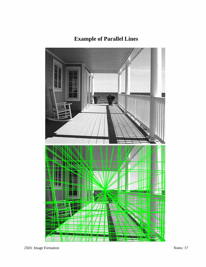
Example of Parallel Lines


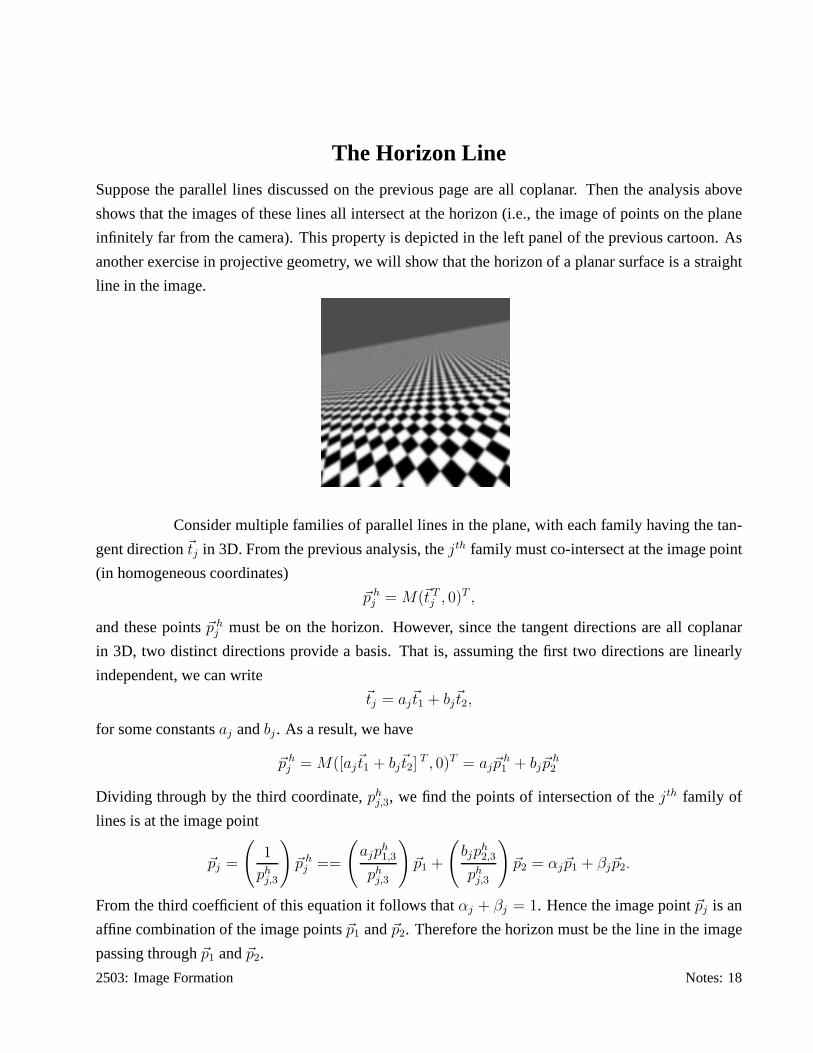
The Horizon Line

Suppose the parallel lines discussed on the previous page are all coplanar. Then the analysis above

shows that the images of these lines all intersect at the horizon (i.e., the image of points on the plane

infinitely far from the camera). This property is depicted inthe left panel of the previous cartoon. As

another exercise in projective geometry, we will show that the horizon of a planar surface is a straight

line in the image.

Consider multiple families of parallel lines in the plane, with each family having the tan-

gent direction~tj in 3D. From the previous analysis, thejth family must co-intersect at the image point

(in homogeneous coordinates)

~p hj = M(~t T

j , 0)T ,

and these points~p hj must be on the horizon. However, since the tangent directions are all coplanar

in 3D, two distinct directions provide a basis. That is, assuming the first two directions are linearly

independent, we can write~tj = aj

~t1 + bj~t2,

for some constantsaj andbj . As a result, we have

~p hj = M([aj

~t1 + bj~t2]

T , 0)T = aj~ph1

+ bj~ph2

Dividing through by the third coordinate,phj,3, we find the points of intersection of thejth family of

lines is at the image point

~pj =

(

1

phj,3

)

~p hj ==

(

ajph1,3

phj,3

)

~p1 +

(

bjph2,3

phj,3

)

~p2 = αj~p1 + βj~p2.

From the third coefficient of this equation it follows thatαj + βj = 1. Hence the image point~pj is an

affine combination of the image points~p1 and~p2. Therefore the horizon must be the line in the image

passing through~p1 and~p2.


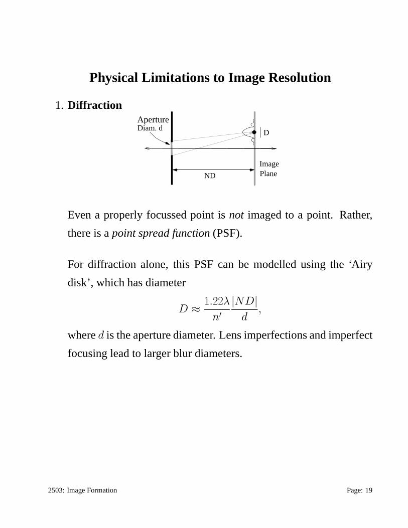
Physical Limitations to Image Resolution

1. Diffraction

Image

ND Plane

DDiam. dAperture

Even a properly focussed point isnot imaged to a point. Rather,

there is apoint spread function (PSF).

For diffraction alone, this PSF can be modelled using the ‘Airy

disk’, which has diameter

D ≈1.22λ

n′

|ND|

d,

whered is the aperture diameter. Lens imperfections and imperfect

focusing lead to larger blur diameters.


Diffraction Limit (cont.)

For example, for human eyes (see Wyszecki & Stiles, Color Science,

1982):

• the index of refraction within the eye isn′ = 1.33;

• the nodal distance is|ND| ≈ 16.7mm (accommodated at∞);

• the pupil diameter isd ≈ 2mm (adapted to bright conditions);

• a typical wavelength isλ ≈ 500nm.

Therefore the diameter of the Airy disk is

D ≈ 4µ = 4 × 10−6m

This compares closely to the diameter of a foveal cone (i.e. the smallest

pixel), which is between1µ and4µ. So, human vision operates at the

diffraction limit.

By the way, a2µ pixel spacing in the human eye corresponds to having

a 300 × 300 pixel resolution of the image of your thumbnail at arm’s

length. Compare this to the typical sizes of images used by machine

vision systems, usually about500 × 500 or less.


2. Photon Noise

The average photon flux (spectral density) at the image (in units of

photons per sec, per unit wavelength, per image area) is

I(λ, ~xI , ~nI)λ

hc

Hereh is Planck’s constant andc is the speed of light.

The photon arrivals can be modelled with Poisson statistics, so the

variance is equal to the mean photon catch.

Even in bright conditions, foveal cones have a significant photon

noise component (a std. dev.≈ 10% of the signal, for unshaded

scenes).

3. Defocus

An improperly focussed lens causes the PSF to broaden. Geomet-

rical optics can be used to get a rough estimate of the size.

4. Motion Blur

Given temporal averaging, the image of a moving point forms a

streak in the image, causing further blur.

Conclude: There is a limit to how small standard cameras and eyes can

be made (but note multi-faceted insect eyes). Human vision operates

close to the physical limits of resolution (ditto for insects).2503: Image Formation Page: 21

Image Formation - University of TorontoImage Formation Goal: Introduce basic concepts in image...

Documents

Transcript of Image Formation - University of TorontoImage Formation Goal: Introduce basic concepts in image...