A THESIS ON

DIGITAL IMAGE COMPRESSION USING DISCRETE

COSINE TRANSFORM & DISCRETE WAVELET

TRANSFORM

Submitted By

Swastik Das Rasmi Ranjan Sethy

Roll No. : 10506008 Roll No. : 10506013

B.Tech : CSE (8th sem) B.Tech : CSE (8th sem)

Guided By

Prof. R. Baliarsingh

Department of Computer Science and Engineering

National Institute of Technology, Rourkela

Rourkela-769008, Orissa, India

DIGITAL IMAGE COMPRESSION USING DISCRETE COSINE

TRANSFORM & DISCRETE WAVELET TRANSFORM

A THESIS SUBMITTED IN PARTIAL FULFILLMENT OF THE

REQUIREMENTS FOR THE DEGREE OF

Bachelor of Technology

In

Computer Science & Engineering

By

Swastik Das

& Rasmi Ranjan Sethy

Under the Guidance of

Prof R. Baliarsingh

Department of Computer Science and Engineering National Institute of Technology Rourkela

Rourkela-769 008, Orissa, India

2009

National Institute of Technology

Rourkela CERTIFICATE

This is to certify that the thesis entitled “IMAGE COMPRESSION USING DCT &

DWT” submitted by Sri Swastik Das(Roll No.10506008) & Sri Rasmi Ranjan Sethy(Roll NO

.10506013) in partial fulfillment of the requirements for the award of Bachelor of Technology

degree in Computer Science & Engineering at the National Institute of Technology,

Rourkela (Deemed University) is an authentic work carried out by them under my supervision

and guidance.

To the best of my knowledge, the matter embodied in the thesis has not been submitted to any

other University/Institute for the award of any Degree or Diploma.

Date: Prof. R Baliarsingh

i

ACKNOWLEDGEMENT

My heart pulsates with the thrill for tendering gratitude to those persons who helped me in

completion of the project.

The most pleasant point of presenting a thesis is the opportunity to thank those who have

contributed to it. Unfortunately, the list of expressions of thank no matter how extensive is

always incomplete and inadequate. Indeed this page of acknowledgment shall never be able to

touch the horizon of generosity of those who tendered their help to me.

First and foremost, I would like to express my gratitude and indebtedness to Prof. R.

Baliarsingh , for his kindness in allowing me for introducing the present topic and for his

inspiring guidance, constructive criticism and valuable suggestion throughout this project

work. I am sincerely thankful to him for his able guidance and pain taking effort in improving

my understanding of this project.

I am also grateful to Prof. Banshidhar Majhi (Head of the Department) for assigning me this

interesting project and for his valuable suggestions and encouragements at various stages of the

work.

An assemblage of this nature could never have been attempted without reference to and

inspiration from the works of others whose details are mentioned in reference section. I

acknowledge my indebtedness to all of them.

Last but not least, my sincere thanks to all my friends who have patiently extended all sorts of

help for accomplishing this undertaking.

DATE:

PLACE:

Swastik Das

Rasmi Ranjan Sethy

Dept. of Computer Science &

Engineering

National Institute of

Technology Rourkela – 769008

ii

ABSTRACT

Image Compression addresses the problem of reducing the amount of data required to

represent the digital image. Compression is achieved by the removal of one or more of

three basic data redundancies: (1) Coding redundancy, which is present when less than

optimal (i.e. the smallest length) code words are used; (2) Interpixel redundancy, which

results from correlations between the pixels of an image & (3) psycho visual redundancy

which is due to data that is ignored by the human visual system (i.e. visually

nonessential information). Huffman codes contain the smallest possible number of code

symbols (e.g., bits) per source symbol (e.g., grey level value) subject to the constraint that

the source symbols are coded one at a time. So, Huffman coding when combined with

technique of reducing the image redundancies using Discrete Cosine Transform (DCT)

helps in compressing the image data to a very good extent.

The Discrete Cosine Transform (DCT) is an example of transform coding. The current

JPEG standard uses the DCT as its basis. The DC relocates the highest energies to the upper

left corner of the image. The lesser energy or information is relocated into other areas. The

DCT is fast. It can be quickly calculated and is best for images with smooth edges like

photos with human subjects. The DCT coefficients are all real numbers unlike the Fourier

Transform. The Inverse Discrete Cosine Transform (IDCT) can be used to retrieve the

image from its transform representation.

The Discrete wavelet transform (DWT) has gained widespread acceptance in signal

processing and image compression. Because of their inherent multi-resolution nature,

wavelet-coding schemes are especially suitable for applications where scalability and

tolerable degradation are important. Recently the JPEG committee has released its new

image coding standard, JPEG-2000, which has been based upon DWT.

iii

List of Acronyms

Acronym Description

DCT Discrete Cosine Transformation DWT Discrete Wavelet Transformation DFT Discrete Fourier Transformation FFT Fast Fourier Transformation FWT Fast Wavelet Transformation JPEG Joint Photographic Expert Group JPEG-2000 Joint Photographic Expert Group-2000 MPEG Moving Pictures Experts Group MSE Mean Square Error PSNR Peak Signal to Noise Ratio SNR Signal-to-noise Ratio ISO International Standards Organization LOT Lapped Orthogonal Transforms IEC International Electro-Technical Commission DPCM Discrete pulse code modulation FAX Facsimile transmission KLT Karhunen Lòeve Transform IDCT Inverse Discrete Cosine Transform FDCT A Forward Discrete Cosine Transform

iv

List of Symbols

Symbol Description

CR Compression ratio RD Relative data redundancy SNRms Mean-square Signal-to-noise ratio erms Root-mean-square error

v

CONTENT Page no

Certificate i

Acknowledgement ii

Abstract iii

List of Acronyms iv

List of Symbols v

CHAPTER :1 Introduction

1.1 Overview 1

1.2 Objectives 1

1.3 OrganiZation of the thesis 2

CHAPTER 2.Image Compression

2.1 Preview 3

2.2 Need of compression 4

2.3 Fundamentals of image compression 5

2.4 Image Compression and Reconstruction 6

2.5 Different classes of compression technique 8

2.6 A typical image coder . 9

2.6.1 Source Encoder (or Linear Transformer) 9

2.6.2 Quantizer 9

2.6.3 Entropy Encoder 9

2.7 Motivation 10

CHAPTER 3. IMAGE COMPRESSION USING DISCRETE COSINE TRANSFORM

Preamble

3.1 The Process 12

3.2 Discrete cosine transform (DCT) equation :- 13 3.3 JPEG Compression 16 3.4 Quantisation 18

3.5 Coding 18

3.5.1 Huffman Coding 19

3.5.2 Huffman Decoding 21

3.6 Result 22

3.6.1 Original input image 22

3.6.2 Image after applying DCT 22

3.6.3 Histogram of the DCT coefficients of the upper half of the image

. before quantization. 23

3.6.4 Histogram of the DCT coefficients of the lower half of the image

. before quantization. 23

3.6.5 Histogram of the DCT coefficients of the upper half of the image .

. after quantization. 24

3.6.6 Histogram of the DCT coefficients of the lower half of the image

. after quantization. 24

3.6.7 Image after compression 25

3.6.8 Parameters associated with the output image (fig.2.4) 26

3.6.9 Parameters associated with the output image(fig.2.5) 26

CHAPTER 4. IMAGE COMPRESSION USING DISCRETE WAVELET TRANSFORM

4.1 What is a Wavelet Transform ? 27

4.2 Why Wavelet-based Compression? 27

4.3 Subband Coding 29

4.3.1 From Subband to Wavelet Coding 30

4.4 Link between Wavelet Transform and Filterbank 30

4.5 An Example of Wavelet Decomposition 31

4.6 Result 33

4.7 Conclusion 34

References 35

LIST OF TABLES

Page no

1.1 Multimedia data types and uncompressed storage space, transmission bandwidth, a

and transmission time required…………………………………………………….4

1.2 Huffman coding ………………………………………………………………… 20

1.3 Parameters associated with the output image at different decomposition level and .

. threshold…………………………………………………………………………..33

LIST OF FIGURES

1.1 Image compression System………………………………………………………..6

1.2 Image decompression System…………………………………………………......7

1.3 A Typical Lossy Signal/Image Encoder………………………………………...…8

1.4 JPEG Encoder……………………………….16

1.5 JPEG Decoder……………………………….17

1.6 Huffman Tree……………………………………………………………………...21 1.7 Original input image(Lena image)………………………………………………...22

1.8 Image after applying DCT……………………………………………………… 22

1.9 Histogram of the DCT coefficients of the upper half of the image before

quantization………………………………………………………………………..23

2.0 Histogram of the DCT coefficients of the lower half of the image before

quantization…………………………………………………………………………23

2.1 Histogram of the DCT coefficients of the upper half of the image after quantization………………………………………………………………………..24 2.2 Histogram of the DCT coefficients of the lower half of the image after quantization………………………………………………………………………..24 2.3 Image after compression…………………………………………………………...25

2.4 Image of Parameters(3.6.8) associated with the output image implemented

in MATLAB…………………………………………………………………………….…26

2.5 Image of Parameters(3.6.9) associated with the output image implemented

in MATLAB………………………………………………………………………………26

2.6 (a) Original Lena Image, and (b) Reconstructed Lena with DC component only, to

show blocking artifacts…………………………………………………………………...28

2.7 Separable 4-subband Filterbank,…………………………………………………...29

2.8 Partition of the Frequency Domain……………………………………………………………..29

2.9 Three level octave-band decomposition of Lena image,………………………………….31

3.0 Spectral decomposition and ordering……………………………………………………..32

Page | 1

Chapter :1

Introduction 1.1 Overview

Uncompressed multimedia (graphics, audio and video) data requires considerable storage capacity and transmission bandwidth. Despite rapid progress in mass-storage density, processor speeds, and digital communication system performance, demand for data storage capacity and data-transmission bandwidth continues to outstrip the capabilities of available technologies. The recent growth of data intensive multimedia-based web applications have not only sustained the need for more efficient ways to encode signals and images but have made compression of such signals central to storage and communication technology.

For still image compression, the `Joint Photographic Experts Group' or JPEG [7]standard

has been established by ISO (International Standards Organization) and IEC (International

Electro-Technical Commission). The performance of these coders generally degrades at low

bit-rates mainly because of the underlying block-based Discrete Cosine Transform (DCT)

scheme. More recently, the wavelet transform has emerged as a cutting edge technology,

within the field of image compression. Wavelet-based coding provides substantial

improvements in picture quality at higher compression ratios.

Over the past few years, a variety of powerful and sophisticated wavelet-based schemes for

image compression, as discussed later, have been developed and implemented. Because of

the many advantages, the top contenders in the upcoming JPEG-2000 standard are all

wavelet-based compression algorithms.

1.2 Objectives

Image Compression addresses the problem of reducing the amount of data required

torepresent the digital image. Compression is achieved by the removal of one or more of

threebasic data redundancies: (1) Coding redundancy, which is present when less than

optimal (i.e.the smallest length) code words are used; (2) Interpixel redundancy, which

results fromcorrelations between the pixels of an image; &/or (3) psycho visual redundancy

which is due todata that is ignored by the human visual system (i.e. visually nonessential

information).Huffman codes contain the smallest possible number of code symbols (e.g.,

bits) per source symbol (e.g., grey level value) subject to the constraint that the source

symbols are coded one at a time. So, Huffman coding when combined with technique of

reducing the image redundancies using Discrete Cosine Transform (DCT) helps in

compressing the image data to a very good extent.

Page | 2

1.3 Organization of the Thesis

Rest of the thesis is organized into the following chapters :

A discussion on Fundamentals of image compression, Different classes of compression

technique ,a typical image coder are given in Chapter 2.

Image compression using discrete cosine transform is proposed in Chapter 3. The objective

is to achieve a reasonable compression ratio as well as better quality of reproduction

of image with a low power consumption. Simulation result shows that a compression

ratio of 2.0026 is achieved.

Image compression using discrete wavelet transform is proposed in Chapter 4.

Parameters associated with the compression process are analysed & the conclusion is given.

Page | 3

Chapter :2

IMAGE COMPRESSION

2.1 Preview

Image compression addresses the problem of reducing the amount of data required to

represent a digital image .The underlying basis of the reduction process is the removal of

redundant data. From a mathematical viewpoint, this amounts to transforming a 2-D pixel

array into a statistically uncorrelated data set .The transformation is applied prior to storage

or transmission of the image. At some later time, the compressed image is decompressed to

reconstruct the original image or approximation of it.

Interest in image compression dates back more than 35 years. The initial focus of research

efforts in this field was on the development of analog methods for reducing video

transmission bandwidth, a process called bandwidth compression. The advent of the digital

computer and subsequent development of advanced integrated circuits, however, caused

interest to shift from analog to digital compression approaches. with the relatively recent

adaption of several key international image compression standards ,the field has undergone

significant growth through the practical application of the theoretic work that began in the

1940s, when C.E Shannon and others first formulated the probabilistic view of information

and its representation , transmission, and compression[1].

Currently image compression is recognized as an “enabling technology”. In addition to the

areas Just mentioned ,image compression is the natural technology for handling the

increased spatial resolution of today’s imaging sensors and evolving broadcast television

standards. Furthermore image compression plays a major role in many important and

diverse applications , including televideo-conferencing ,remote sensing(the use of satellite

imagery for weather and other earth –resource applications), document and medical imaging

,facsimile transmission(FAX)[3], and the control of remotely piloted vehicles in military ,

space and hazardous waste management applications.

Page | 4

2.2 Need of compression

The figures in Table 1.1 show the qualitative transition from simple text to full-motion video

data and the disk space, transmission bandwidth, and transmission time needed to store and

transmit such uncompressed data.

Multimedia

Data Size/Duration

Bits/Pixel

or

Bits/Sample

Uncompressed

Size

(B for bytes)

Transmission

Bandwidth

(b for bits)

Transmission

Time (using a

28.8K

Modem)

A page of

text 11'' x 8.5''

Varying

resolution 4-8 KB

32-64

Kb/page 1.1 - 2.2 sec

Telephone

quality

speech

10 sec 8 bps 80 KB 64 Kb/sec 22.2 sec

Grayscale

Image 512 x 512 8 bpp 262 KB 2.1 Mb/image 1 min 13 sec

Color Image 512 x 512 24 bpp 786 KB 6.29

Mb/image 3 min 39 sec

Medical

Image 2048 x 1680 12 bpp 5.16 MB

41.3

Mb/image 23 min 54 sec

SHD Image 2048 x 2048 24 bpp 12.58 MB 100

Mb/image 58 min 15 sec

Full-motion

Video

640 x 480, 1

min

(30

frames/sec)

24 bpp 1.66 GB 221 Mb/sec 5 days 8 hrs

Table 1.1 Multimedia data types and uncompressed storage space, transmission

bandwidth, and transmission time required. The prefix kilo- denotes a factor of 1000

rather than 1024.

The examples above clearly illustrate the need for sufficient storage space, large

transmission bandwidth, and long transmission time for image, audio, and video data. At the

present state of technology, the only solution is to compress multimedia data before its

storage and transmission, and decompress it at the receiver for play back. For example, with

a compression ratio of 32:1, the space, bandwidth, and transmission time requirements can

be reduced by a factor of 32, with acceptable quality[2].

other hand, first transforms the image from its spatial domain representation to a different

type of representation using some well-known transform and then codes the transformed

values (coefficients). This method provides greater data compression compared to predictive

methods, although at the expense of greater computation.

Page | 5

2.3 Fundamentals of image compression

The term data compression refers to the process of reducing the amount of data required to

represent a given quantity of information. A common characteristic of most images is that

the neighboring pixels are correlated and therefore contain redundant information. The

foremost task then is to find less correlated representation of the image. Two fundamental

components of compression are redundancy and irrelevancy reduction. Redundancy

reduction aims at removing duplication from the signal source (image/video). Irrelevancy

reduction omits parts of the signal that will not be noticed by the signal receiver, namely the

Human Visual System (HVS).

It is not an abstract concept but a mathematically quantifiable entity.If n1 and n2 denote the

number of information-carrying units in the two data sets that represent the same

information , the relative data redundancy RD of the first data set (the one characterized by

n1)can be defined as

RD = 1 - 1/ CR

Where CR , commonly called the compression ratio,is

CR = n1/n2 .

For the case n2 = n1 and RD = 0, indicating that (relative to the second data set)the first

representation of the information contains no redundant data. When n2<< n1. CR -> ∞

and RD ->1,implying significant compression and highly redundant data. When n2 >> n1,

CR ->0and RD -> -∞ ,indicating that the second data set contains much more data than the

original representation. Generally CR =10(10:1) defines that the first data set has 10

information carrying units for every 1 unit in the second or compressed data set. Thus the

corresponding redundancy of 0.9 means 90 percent of the data in the first data set is

redundant with respect to the second one.[1]

In order to be useful, a compression algorithm has a corresponding

decompression algorithm that reproduces the original file once the compressed file is

given. There have been many types of compression algorithms developed. These

algorithms fall into two broad types, lossless algorithms and lossy algorithms. A

lossless algorithm reproduces the data exactly same as the original one. A lossy

algorithm, as its name implies, loses some data. Data loss may be unacceptable in

Page | 6

many applications. For example, text compression must be lossless because a very

small difference can result in statements with totally different meanings. There are also

many situations where loss may be either unnoticeable or acceptable. In image

compression, for example, the exact reconstructed value of each sample of the image

2.4 Image Compression and Reconstruction

Three basic data redundancies can be categorized in the image compression

standard.

1. Spatial redundancy due to the correlation between neighboring pixels.

2. Spectral redundancy due to correlation between the color components.

3. Psycho-visual redundancy due to properties of the human visual system.

The spatial and spectral redundancies are present because certain spatial and

spectral patterns between the pixels and the color components are common to each

other, whereas the psycho-visual redundancy originates from the fact that the human

eye is insensitive to certain spatial frequencies. The principle of image compression

algorithms are (i) reducing the redundancy in the image data and (or) (ii) producing a

reconstructed image from the original image with the introduction of error that is

insignificant to the intended applications. The aim here is to obtain an acceptable

representation of digital image while preserving the essential information contained

in that particular data set.[2]

Original

Transform Quantisation Lossless

Compressed

Image

Figure 1.1 Image

compression System

Coding Image

Page | 7

The problem faced by image compression is very easy to define, as

demonstrated in figure 1.1. First the original digital image is usually transformed into

another domain, where it is highly de-correlated by using some transform. This de-

correlation concentrates the important image information into a more compact form.

The compressor then removes the redundancy in the transformed image and stores it

into a compressed file or data stream. In the second stage, the quantisation block

reduces the accuracy of the transformed output in accordance with some pre- established

fidelity criterion. Also this stage reduces the psycho-visual redundancy of the input

image. Quantisation operation is a reversible process and thus may be omitted when

there is a need of error free or lossless compression. In the final stage of the data

compression model the symbol coder creates a fixed or variable-length code to

represent the quantiser output and maps the output in accordance with the code.

Generally a variable-length code is used to represent the mapped and quantised data set. It

assigns the shortest code words to the most frequently occurring output values and thus

reduces coding redundancy. The operation in fact is a reversible one.

The decompression reverses the compression process to produce the

recovered image as shown in figure 1.2. The recovered image may have lost some

information due to the compression, and may have an error or distortion compared to

the original image.

Compressd

Image

Inverse

Transform dequantisation

Figure 1.2 Image

decompression System

Lossless

Decodig

Reconstructed

Image

Page | 8

2.5 DIFFERENT CLASSES OF COMPRESSION TECHNIQUES.

Two ways of classifying compression techniques are mentioned here.

(a) Lossless vs. Lossy compression: In lossless compression schemes, the reconstructed

image, after compression, is numerically identical to the original image. However lossless

compression can only a achieve a modest amount of compression. An image reconstructed

following lossy compression contains degradation relative to the original. Often this is

because the compression scheme completely discards redundant information. However,

lossy schemes are capable of achieving much higher compression. Under normal viewing

conditions, no visible loss is perceived (visually lossless).

(b) Predictive vs. Transform coding: In predictive coding, information already sent or

available is used to predict future values, and the difference is coded. Since this is done in

the image or spatial domain, it is relatively simple to implement and is readily adapted to

local image characteristics. Differential Pulse Code Modulation (DPCM) is one particular

example of predictive coding [3]. Transform coding, on the other hand, first transforms the

image from its spatial domain representation to a different type of representation using some

well-known transform and then codes the transformed values (coefficients). This method

provides greater data compression compared to predictive methods, although at the expense

of greater computation.

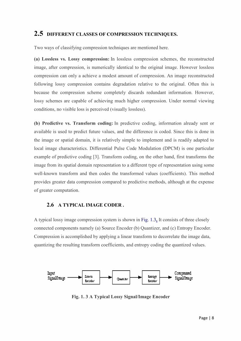
2.6 A TYPICAL IMAGE CODER .

A typical lossy image compression system is shown in Fig. 1.3. It consists of three closely

connected components namely (a) Source Encoder (b) Quantizer, and (c) Entropy Encoder.

Compression is accomplished by applying a linear transform to decorrelate the image data,

quantizing the resulting transform coefficients, and entropy coding the quantized values.

Fig. 1. 3 A Typical Lossy Signal/Image Encoder

Page | 9

2.6.1 Source Encoder (or Linear Transformer)

Over the years, a variety of linear transforms have been developed which include Discrete

Fourier Transform (DFT), Discrete Cosine Transform (DCT) , Discrete Wavelet Transform

(DWT) and many more, each with its own advantages and disadvantages.

2.6.2 Quantizer

A quantizer simply reduces the number of bits needed to store the transformed coefficients

by reducing the precision of those values. Since this is a many-to-one mapping, it is a lossy

process and is the main source of compression in an encoder. Quantization can be

performed on each individual coefficient, which is known as Scalar Quantization (SQ).

Quantization can also be performed on a group of coefficients together, and this is known as

Vector Quantization (VQ) [6] . Both uniform and non-uniform quantizers can be used

depending on the problem at hand. .

2.6.3 Entropy Encoder

An entropy encoder further compresses the quantized values losslessly to give better overall

compression. It uses a model to accurately determine the probabilities for each quantized

value and produces an appropriate code based on these probabilities so that the resultant

output code stream will be smaller than the input stream. The most commonly used entropy

encoders are the Huffman encoder and the arithmetic encoder, although for applications

requiring fast execution, simple run-length encoding (RLE) has proven very effective [6].

It is important to note that a properly designed quantizer and entropy encoder are absolutely

necessary along with optimum signal transformation to get the best possible compression.

Page | 10

2.7 Motivation

Image compression is an important issue in digital image processing and

finds extensive applications in many fields. This is the basic operation performed

frequently by any digital photography technique to capture an image. For longer use

of the portable photography device it should consume less power so that battery life

will be more. To improve the Conventional techniques of image compressions using

the DCT have already been reported and sufficient literatures are available on this.

The JPEG is a lossy compression scheme, which employs the DCT as a tool and used

mainly in digital cameras for compression of images. In the recent past the demand

for low power image compression is growing. As a result various research workers

are actively engaged to evolve efficient methods of image compression using latest

digital signal processing techniques. The objective is to achieve a reasonable

compression ratio as well as better quality of reproduction of image with a low

power consumption. Keeping these objectives in mind the research work in the

present thesis has been undertaken. In sequel the following problems have been

investigated.

Page | 11

Chapter : 3

IMAGE COMPRESSION USING DISCRETE COSINE TRANSFORM

Preview:

Discrete cosine transform (DCT) is widely used in image processing, especially for

compression. Some of the applications of two-dimensional DCT involve still image

compression and compression of individual video frames, while multidimensional DCT

is mostly used for compression of video streams. DCT is also useful for transferring

multidimensional data to frequency domain, where different operations, like spread-

spectrum, data compression, data watermarking, can be performed in easier and more

efficient manner. A number of papers discussing DCT algorithms is available in the

literature that signifies its importance and application.[5]

Hardware implementation of parallel DCT transform is possible, that would give higher

throughput than software solutions. Special purpose DCT hardware decreases the

computational load from the processor and therefore improves the performance of

complete multimedia system. The throughput is directly influencing the quality of

experience of multimedia content. Another important factor that influences the

quality is the finite register length effect that affects the accuracy of the forward-inverse

transformation process.

Page | 12

Hence, the motivation for investigating hardware specific DCT algorithms is clear. As 2-

D DCT algorithms are the most typical for image compression, the main focus of this

chapter will be on the efficient hardware implementations of 2-D DCT based

compression by decreasing the number of computations, increasing the accuracy of

reconstruction, and reducing the chip area. This in return reduces the power

consumption of the compression technique. As the number of applications that require

higher-dimensional DCT algorithms are growing, a special attention will be paid to the

algorithms that are easily extensible to higher dimensional cases.

The JPEG standard has been around since the late 1980's and has been an effective

first solution to the standardization of image compression. Although JPEG has some

very useful strategies for DCT quantization and compression, it was only developed for

low compressions. The 8 × 8 DCT block size was chosen for speed(which is less of

an issue now, with the advent of faster processors) not for performance. The JPEG

standard will be briefly explained in this chapter to provide a basis to understand the new

DCT related work [7].

3.1 The Process:-

The following is the general overview of the JPEG process.Later we will go through the a

detailed tour of JPEG’s method so that a more comprehensive understanding of the process

may be acquired.

1.The image is broken into 8*8 blocks of pixels.

2. Working from left to right, top to bottom, the DCT is applies to each block.

3. Each block is compressed through quantization.

4.The array of compressed blocks that constitute the image is stored in a drastically reduced

amount of space.

5. When desired the image is constructed through decompression, a process that uses the

Inverse Discrete Cosine Transform(IDCT).

Page | 13

3.2 DISCRETE COSINE TRANSFORM (DCT) EQUATION :-

The DCT is a widely used transformation in transformation for data compression. It is an

orthogonal transform, which has a fixed set of (image independent) basis functions, an

efficient algorithm for computation, and good energy compaction and correlation reduction

properties. Ahmed et al found that the Karhunen Lòeve Transform (KLT) basis function of

a first order Markov image closely resemble those of the DCT [7]. They become identical as

the correlation between the adjacent pixel approaches to one.

The DCT belongs to the family of discrete trigonometric transform, which has 16 members

[44]. The 1D DCT of a 1× N vector x(n) is defined as

where k = 0,1,2,..., N −1 and

The original signal vector x(n) can be reconstructed back from the DCT coefficients

Y[k ] using the Inverse DCT (IDCT) operation and can be defined as

where n = 0,1,2,..., N −1

Page | 14

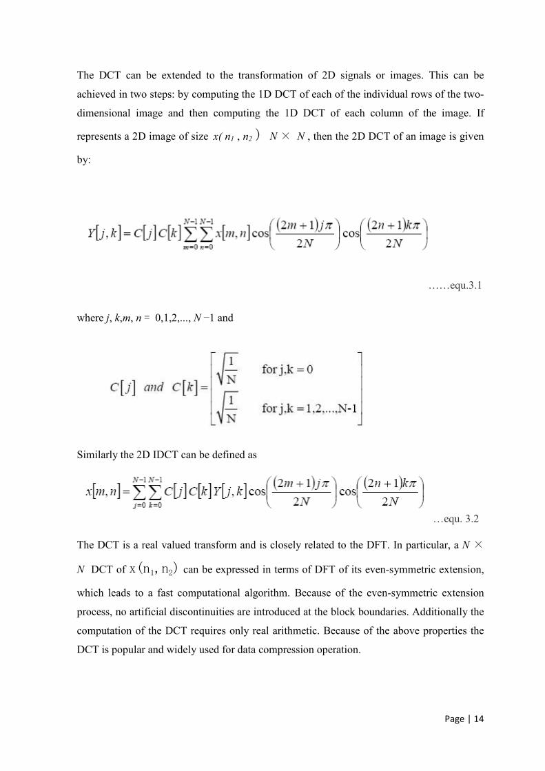
The DCT can be extended to the transformation of 2D signals or images. This can be

achieved in two steps: by computing the 1D DCT of each of the individual rows of the two-

dimensional image and then computing the 1D DCT of each column of the image. If

represents a 2D image of size x( n1 , n2 ) N × N , then the 2D DCT of an image is given

by:

……equ.3.1

where j, k,m, n = 0,1,2,..., N −1 and

Similarly the 2D IDCT can be defined as

…equ. 3.2

The DCT is a real valued transform and is closely related to the DFT. In particular, a N ×

N DCT of x(n1,n2) can be expressed in terms of DFT of its even-symmetric extension,

which leads to a fast computational algorithm. Because of the even-symmetric extension

process, no artificial discontinuities are introduced at the block boundaries. Additionally the

computation of the DCT requires only real arithmetic. Because of the above properties the

DCT is popular and widely used for data compression operation.

Page | 15

The DCT presented in equations (3.1) and (3.2) is orthonormal and perfectly reconstructing

provided the coefficients are represented to an infinite precision. This means that when the

coefficients are compressed it is possible to obtain a full range of compressions and image

qualities. The coefficients of the DCT are always quantized for high compression, but DCT

is very resistant to quantisation errors due to the statistics of the coefficients it produces.

The coefficients of a DCT are usually linearly quantised by dividing by a predetermined

quantisation step.

The DCT is applied to image blocks N x N pixels in size (where N is usually multiple of 2)

over the entire image. The size of the blocks used is an important factor since they

determine the effectiveness of the transform over the whole image. If the blocks are too

small then the images is not effectively decorrelated but if the blocks are too big then local

features are no longer exploited. The tiling of any transform across the image leads to

artifacts at the block boundaries. The DCT is associated with blocking artifact since the

JPEG standard suffers heavily from this at higher compressions. However the DCT is

protected against blocking artifact as effectively as possible, without interconnecting blocks,

since the DCT basis functions all have a zero gradient at the edges of their blocks. This

means that only the DC level significantly affects the blocking artifact and this can then be

targeted. Ringing is a major problem in DCT operation. When edges occur in an image DCT

relies on the high frequency components to make the image shaper. However these high

frequency components persist across the whole block and although they are effective at

improving the edge quality they tend to 'ring' in the flat areas of the block.

This ringing effect increases, when larger blocks are used, but larger blocks are better in

compression terms, so a trade off is usually established [1].

Page | 16

3.3 JPEG Compression

The JPEG (Joint Photographic Experts Group) standard has been around

for some time and is the only standard for lossy still image compression. There

are quite a lot of interesting techniques used in the JPEG standard and it is

important to give an overview of how JPEG works. There are several variations of

JPEG, but only the 'baseline' method is discussed here.

8 x 8 blocks

DCT – Based Encoder

FDCT Quantizer Huffman

Encoder

Source Image

Data

Table

Specifications

Table

Specifications

Figure 1.4: JPEG Encoder

As shown in the figure 3.1, the image is first partitioned into non-overlapping

8 × 8 blocks. A Forward Discrete Cosine Transform (FDCT) is applied to each block

to convert the spatial domain gray levels of pixels into coefficients in frequency

domain. To improve the precision of the DCT the image is 'zero shifted', before the

DCT is applied. This converts a 0

→ 255 image intensity range to a -128

→ 127

range, which works more efficiently with the DCT. One of these transformed values

is referred to as the DC coefficient and the other 63 as the AC coefficients [4].

After the computation of DCT coefficients, they are normalized with

different scales according to a quantization table provided by the JPEG standard

conducted by psychovisual evidence. The quantized coefficients are rearranged in a

zigzag scan order for further compressed by an efficient lossless coding algorithm

such as runlength coding, arithmetic coding, Huffman coding. The decoding process

is simply the inverse process of encoding as shown in figure 1.5.

Page | 17

The decoding process is simply the inverse process of encoding as shown in figure 1.5.

DCT – Based Decoder

Compressed

Huffman

Decoder

Dequantizer IDCT

Image Data Reconstruct Table

Specifications

Figure 1.5 : JPEG Decoder

Table

Specifications

Image Data

Page | 18

3.4 QUANTISATION

DCT-based image compression relies on two techniques to reduce the data required to represent

the image. The first is quantization of the image's DCT coefficients; the second is entropy coding

of the quantized coefficients. Quantization is the process of reducing the number of possible

values of a quantity, thereby reducing the number of bits needed to represent it. In lossy image

compression the transformation decompose the image into uncorrelated parts projected on

orthogonal basis of the transformation. These basis are represented by eigenvectors which are

independent and orthogonal in nature. Taking inverse of the transformed values will result in the

retrieval of the actual image data. For compression of the image, the independent characteristic

of the transformed coefficients are considered, truncating some of these coefficients will not

affect the others. This truncation of the transformed coefficients is actually the lossy process

involved in compression and known as quantization . So we can say that DCT is perfectly

reconstructing, when all the coefficients are calculated and stored to their full resolution. For

high compression, the DCT coefficients are normalized by different scales, according to the

quantization matrix [6].

Vector quantization, (VQ) mainly used for reducing or compressing the image data . Application

VQ on images for compression started from early 1975by Hilbert mainly for the coding of

multispectral Landsat imaginary.

3.5 CODING

After the DCT coefficients have been quantized, the DC coefficients are DPCM coded and then

they are entropy coded along with the AC coefficients. The quantized AC and DC coefficient

values are entropy coded in the same way, but because of the long runs in the AC coefficient, an

additional run length process is applied to them to reduce their redundancy.

Page | 19

The quantized coefficients are all rearranged in a zigzag order as shown in figure 3.4. The run

length in this zigzag order is described by a RUN-SIZE symbol. The RUN is a count of how

many zeros occurred before the quantized coefficient and the SIZE symbol is used in the same

way as it was for the DC coefficients, but on their AC counter parts. The two symbols are

combined to form a RUN-SIZE symbol and this symbol is then entropy coded. Additional bits

are also transmitted to specify the exact value of the quantized coefficient. A size of zero in the

AC coefficient is used to indicate that the rest of the 8 × 8 block is zeros (End of Block or

EOB) [7].

3.5.1 HUFFMAN CODING:

Huffman coding is an efficient source coding algorithm for source symbols that are not equally

probable. A variable length encoding algorithm was suggested by Huffman in 1952, based on

the source symbol probabilities P(xi), i=1,2…….,L . The algorithm is optimal in the sense that

the average number of bits required to represent the source symbols is a minimum provided the

prefix condition is met. The steps of Huffman coding algorithm are given below [7]:

1. Arrange the source symbols in increasing order of heir probabilities.

Page | 20

2. Take the bottom two symbols & tie them together as shown in Figure 3. Add the

probabilities of the two symbols & write it on the combined node. Label the two branches with a

‘1’ & a ‘0’ as depicted in Figure 3

3. Treat this sum of probabilities as a new probability associated with a new symbol. Again

pick the two smallest probabilities, tie them together to form a new probability. Each time we

perform the combination of two symbols we reduce the total number of symbols by

one. Whenever we tie together two probabilities (nodes) we label the two branches with a ‘0’ &

a ‘1’.

4. Continue the procedure until only one procedure is left (& it should be one if

your addition is correct). This completes the construction of the Huffman Tree.

5. To find out the prefix codeword for any symbol, follow the branches from the final node

back to the symbol. While tracing back the route read out the labels on the branches. This is the

codeword for the symbol.

The algorithm can be easily understood using the following example : TABLE 1.2

Symbol Probability Codeword Code length

X1 0.46 1 1

X2 0.30 00 2

X3 0.12 010 3

X4 0.06 0110 4

X5 0.03 01110 5

X6 0.02 011110 6

X7 0.01 011111 6

Page | 21

FIGURE: 1.6

Huffman Coding for Table

3.5.2 HUFFMAN DECODING

The Huffman Code in Table 1 & FIGURE 4 is an instantaneous uniquely decodable block code. It is a block code because each source symbol is mapped into a fixed sequence of code symbols. It is instantaneous because each codeword in a string of code symbols can be decoded without referencing succeeding symbols. That is, in any given Huffman code, no codeword is a prefix of any other codeword. And it is uniquely decodable because a string of code symbols can be decoded only in one way. Thus any string of Huffman encoded symbols can be decoded by examining the individual symbols of the string in left to right manner. Because we are using an instantaneous uniquely decodable block code, there is no need to insert delimiters between the encoded pixels.

For Example consider a 19 bit string 1010000111011011111 which can be decoded uniquely as

x1 x3 x2 x4 x1 x1 x7 [7].

A left to right scan of the resulting string reveals that the first valid code word is 1 which is a code symbol for, next valid code is 010 which corresponds to x1, continuing in this manner, we obtain a completely decoded sequence given by x1 x3 x2 x4 x1 x1 x7.

Page | 22

3.6 RESULT :-

3.6.1 - Original input image(1.7)

3.6.2 - Image after applying DC (1.8)

Page | 23

3.6.3 - Histogram of the DCT coefficients of the upper half of the image before

quantization(1.9)

3.6.4 Histogram of the DCT coefficients of the lower half of the image before

quantization.(2.0)

Page | 24

3.6.5 Histogram of the DCT coefficients of the upper half of the image after

quantization.(2.1)

3.6.6 Histogram of the DCT coefficients of the lower half of the image after

quantization.(2.2)

Page | 25

3.6.7 - Image after compression(2.3)

Page | 26

3.6.8 - Parameters associated with the output image(2.4)

3.6.9 - Parameters associated with the output image(2.5)

Page | 27

Chapter : 4

IMAGE COMPRESSION USING DISCRETE WAVELET TRANSFORM :-

The wavelet transform (WT) has gained widespread acceptance in signal processing and image

compression.Because of their inherent multi-resolution nature, wavelet-coding schemes are

especially suitable for applications where scalability and tolerable degradation are

important.Recently the JPEG committee has released its new image coding standard, JPEG-

2000, which has been based upon DWT [1].

4.1 What is a Wavelet Transform ?

Wavelets are functions defined over a finite interval and having an average value of zero. The

basic idea of the wavelet transform is to represent any arbitrary function (t) as a superposition of

a set of such wavelets or basis functions. These basis functions or baby wavelets are obtained

from a single prototype wavelet called the mother wavelet, by dilations or contractions (scaling)

and translations (shifts). The Discrete Wavelet Transform of a finite length signal x(n) having N

components, for example, is expressed by an N x N matrix.

4.2 Why Wavelet-based Compression?

Despite all the advantages of JPEG compression schemes based on DCT namely simplicity,

satisfactory performance, and availability of special purpose hardware for implementation, these

are not without their shortcomings. Since the input image needs to be ``blocked,'' correlation

across the block boundaries is not eliminated. This results in noticeable and annoying ``blocking

artifacts'' particularly at low bit rates as shown in Fig 2.6 . Lapped Orthogonal Transforms (LOT)

[9] attempt to solve this problem by using smoothly overlapping blocks. Although blocking

effects are reduced in LOT compressed images, increased computational complexity of such

algorithms do not justify wide replacement of DCT by LOT.

Page | 28

(a)

(b)

Fig. 2.6 (a) Original Lena Image, and (b) Reconstructed Lena with DC component only,

to show blocking artifacts

Over the past several years, the wavelet transform has gained widespread acceptance in signal

processing in general, and in image compression research in particular. In many applications

wavelet-based schemes (also referred as subband coding) outperform other coding schemes like

the one based on DCT. Since there is no need to block the input image and its basis functions

have variable length, wavelet coding schemes at higher compression avoid blocking artifacts.

Wavelet-based coding is more robust under transmission and decoding errors, and also facilitates

progressive transmission of images. In addition, they are better matched to the HVS

characteristics. Because of their inherent multiresolution nature [9], wavelet coding schemes are

especially suitable for applications where scalability and tolerable degradation are important.

Page | 29

4.3 Subband Coding

he fundamental concept behind Subband Coding (SBC) is to split up the frequency band of a signal

(image in our case) and then to code each subband using a coder and bit rate accurately matched to

the statistics of the band. SBC has been used extensively first in speech coding and later in image

coding [12] because of its inherent advantages namely variable bit assignment among the subbands

as well as coding error confinement within the subbands.

Fig. 2.7 Separable 4-subband Filterbank,

Fig 2.8 . Partition of the Frequency Domain.

Page | 30

ods and O'Neil [12] used a separable combination of one-dimensional Quadrature Mirror

Filterbanks (QMF) to perform a 4-band decomposition by the row-column approach as shown

in Fig. 2.7 Corresponding division of the frequency spectrum is shown in Fig. 2.8 . The process

can be iterated to obtain higher band decomposition filter trees. At the decoder, the subband

signals are decoded, upsampled and passed through a bank of synthesis filters and properly

summed up to yield the reconstructed image.

4.3.1 From Subband to Wavelet Coding

Over the years, there have been many efforts leading to improved and efficient design of

filterbanks and subband coding techniques. Since 1990, methods very similar and closely related

to subband coding have been proposed by various researchers under the name of Wavelet

Coding (WC) using filters specifically designed for this purpose [12]. Such filters must meet

additional and often conflicting requirements . These include short impulse response of the

analysis filters to preserve the localization of image features as well as to have fast computation,

short impulse response of the synthesis filters to prevent spreading of artifacts (ringing around

edges) resulting from quantization errors, and linear phase of both types of filters since nonlinear

phase introduce unpleasant waveform distortions around edges. Orthogonality is another useful

requirement since orthogonal filters, in addition to preservation of energy, implement a unitary

transform between the input and the subbands. But, as in the case of 1-D, in two-band Finite

Impulse Response (FIR) systems linear phase and orthogonality are mutually exclusive, and so

orthogonality is sacrificed to achieve linear phase.

4.4 Link between Wavelet Transform and Filterbank

Construction of orthonormal families of wavelet basis functions can be carried out in continuous

time. However, the same can also be derived by starting from discrete-time filters. Daubechies

[9] was the first to discover that the discrete-time filters or QMFs can be iterated and under

certain regularity conditions will lead to continuous-time wavelets. This is a very practical and

extremely useful wavelet decomposition scheme, since FIR discrete-time filters can be used to

implement them. It follows that the orthonormal bases in correspond to a subband coding

scheme with exact reconstruction property, using the same FIR filters for reconstruction as for

decomposition. So, subband coding developed earlier is in fact a form of wavelet coding in

disguise. Wavelets did not gain popularity in image coding until Daubechies established this link

Page | 31

in late 1980s. Later a systematic way of constructing a family of compactly supported

biorthogonal wavelets was developed by Cohen, Daubechies, and Feauveau (CDF) . Although

the design and choice of various filters and the construction of different wavelets from the

iteration of such filters are very important, it is beyond the scope of this article.

4.5 An Example of Wavelet Decomposition

There are several ways wavelet transforms can decompose a signal into various subbands. These

include uniform decomposition, octave-band decomposition, and adaptive or wavelet-packet

decomposition [12]. Out of these, octave-band decomposition is the most widely used. This is a

non-uniform band splitting method that decomposes the lower frequency part into narrower

bands and the high-pass output at each level is left without any further decomposition. Fig. 2.9

shows the various subband images of a 3-level octave-band decomposed Lena using the popular

CDF-9/7 [7] biorthogonal wavelet.

Fig 2.9 Three level octave-band decomposition of Lena image,

Page | 32

Fig 3.0 Spectral decomposition and ordering.

Most of the subband and wavelet coding schemes can also be described in terms of the general

framework depicted as in Fig. 1. The main difference from the JPEG standard is the use of DWT

rather than DCT. Also, the image need not be split into 8 x 8 disjoint blocks. Of course, many

enhancements have been made to the standard quantization and encoding techniques to take

advantage of how the wavelet transforms works on an image and the properties and statistics of

transformed coefficients so generated.

Page | 33

4.6 Result :-

Image size Decomposition

Lavel

Threshhold Compression

ratio

256 x 256 3 40 16.1759

256 x 256 3 60 21.6558

256 x 256 3 80 25.9193

256 x 256 4 40 15.7964

256 x 256 4 60 22.4193

256 x 256 4 80 28.9469

256 x 256 5 40 14.9430

256 x 256 5 60 21.3887

256 x 256 5 80 28.1812

Table 1.3 Parameters associated with the output image at different

decomposition level and threshold

Page | 34

4.7 Conclusion :-

Image compression is of prime importance in Real time applications like video conferencing

where data are transmitted through a channel.

Using JPEG standard DCT is used for mapping which reduces theinterpixel

redundanciesfollowed by quantization which reduces the psychovisual redundancies then

coding redundanciy is reduced by the use of optimal code word having minimum average

length.

In JPEG 2000 standard of image compression DWT is used for mapping, allother methods

remaining same.DWT is more general and efficient than DCT due to the following result:-

� No need to divide the input coding into non-overlapping 2-D blocks, it has higher

compression ratios avoid blocking artifacts.

� Allows good localization both in time and spatial frequency domain.

� Transformation of the whole image� introduces inherent scaling

� Better identification of which data is relevant to human perception� higher

compression ratio

Page | 35

References:

[1] R. C. Gonzalez and R. E. Woods, “Digital Image Processing”, Reading. MA:

Addison Wesley, 2004.

[2] David Salomon, Data Compression, The Complete Reference, 2nd Edition

Springer-Verlag 1998.

[3] Digital Compression and coding of Continuous-tone still images, part 1,

requirements and Guidelines. ISO/IEC JTC1 Draft International Standard

10918-1, Nov. 1991.

[4] G. K. Wallace, “The JPEG Still Picture Compression Standard”, IEEE Trans.

On Consumer Electronics, vol.38, No.1, pp. xviii – xxxiv, Feb 1992.

[5] S. Martucea, “Symmetric convolution and the discrete sine and cosine

transform”, IEEE Transaction on Signal Processing, vol. 42, p. 1038-1051,

May’ 1994.

[6] R. M. Gray, D. L. Neuhoff, “Quantization”, IEEE Trans. Inform. Theory, Vol.

44, No. 6, 1998.

[7] N. Ahmed, T. Natrajan, and K. R. Rao, “Discrete Cosine Transform”, IEEE

Transactions on Computers, vol. 23, July 1989.

[8] Pennebaker, W. B. and Mitchell, J. L. JPEG - Still Image Data Compression Standards,

Van Nostrand Reinhold, 1993.

[9] http://en.wikipedia.org/wiki/Discrete_cosine_transform

[10] Rao, K. R. and Yip, P. Discrete Cosine Transforms - Algorithms, Advantages, Applications,

Academic Press, 1990.

[11] Gersho, A. and Gray, R. M. Vector Quantization and Signal Compression, Kluwer Academic

. publishers

[12] Strang, G. and Nguyen, T. Wavelets and Filter Banks, Wellesley-Cambridge Press, Wellesley, MA,

. 1996 http://www-math.mit.edu/~gs/books/wfb.html.