REVIEW

Image co-localization – co-occurrence versus correlationJesse S. Aaron, Aaron B. Taylor and Teng-Leong Chew*

ABSTRACTFluorescence image co-localization analysis is widely utilized tosuggest biomolecular interaction. However, there exists someconfusion as to its correct implementation and interpretation. Inreality, co-localization analysis consists of at least two distinct sets ofmethods, termed co-occurrence and correlation. Each approach hasinherent and often contrasting strengths and weaknesses. Yet,neither one can be considered to always be preferable for any givenapplication. Rather, each method is most appropriate for answeringdifferent types of biological question. This Review discusses the mainfactors affecting multicolor image co-occurrence and correlationanalysis, while giving insight into the types of biological behavior thatare better suited to one approach or the other. Further, the limits ofpixel-based co-localization analysis are discussed in the context ofincreasingly popular super-resolution imaging techniques.

KEY WORDS: Image analysis, Manders, Pearson, Co-localization,Fluorescence microscopy

IntroductionA common task in cell biology consists of assessing to what extenttwo biomolecules or structures are associated with each other withina cell. Optical microscopy offers a sensitive and specific means toinfer such relationships. While various distinct approaches thatattempt to characterize biomolecular associations from multi-colorfluorescence images have been developed, they are all collectivelyreferred to as co-localization analysis. Previous reviews on thissubject have generally given a survey of various co-localizationmethods, with recommendations for use based on imagecharacteristics (Dunn et al., 2011; Bolte and Cordelieres, 2006;Zinchuk and Grossenbacher-Zinchuk, 2001; Costes et al., 2004;Zinchuk et al., 2007), or advocated for the superiority of oneapproach over another (Adler and Parmryd, 2010). However, thevarious methods discussed here and previously measure two distinctphenomena: co-occurrence and correlation. The former describesthe extent of spatial overlap between two fluorophores. The latterdetermines the degree to which the abundance of two spatiallyoverlapping fluorophores are related to each other. Determining themost appropriate metric, therefore, should be guided by the nature ofthe question being posed. Co-occurrence measurements are oftenbest utilized to determine what proportion of a molecule is presentwithin particular area, compartment or organelle. It does not giveinsight into any concentration relationship between two molecules.Correlation analysis is most applicable when assessing a functionalor stoichiometric relationship between two overlapping species. Itdoes not, however, measure the extent of their spatial co-occurrence.Both measures can supply complementary information about a

biological system. This Review explores how co-localization can bemore strategically employed. We outline strengths and pitfalls ofcorrelation and co-occurrence, both in terms of what phenomenathey measure, as well as common sources of inaccuracies. Finally,we relate these methods to emerging super-resolution imagingtechniques and introduce new approaches based on spatial pointstatistics.

Prerequisites for analysisIt is important to note that neither image correlation norco-occurrence are direct measures of molecular interaction. Theresolving power of a microscope is, conventionally, limited toapproximately half the wavelength of emitting light (Abbe, 1873),while typical interaction distances between bio-molecules are<10 nm. Even with the advent of super-resolution imagingtechniques, intramolecular interactions cannot be unambiguouslyobserved. Only nearfield biophysical techniques, such as Försterresonant energy transfer (FRET), can be used to directly measuremolecular interactions (Truong and Ikura, 2001; Piston andKremers, 2007). Nevertheless, correlation and co-occurrence offera means to infer such relationships.

In this context, optimized sample preparation (Wysocki andLavis, 2011; Grimm et al., 2015; Shaner et al., 2005; Chudakovet al., 2010) and proper image acquisition settings are both essentialfor accurate analysis (North, 2006; Waters, 2009; Stelzer, 1998;Nakamura, 2005). In addition, post-acquisition corrections shouldbe made for inhomogeneous illumination (Sternberg, 1983;Dickinson et al., 2002; Leong et al., 2003). Co-registration of thecomponent images either due to chromatic aberration, focal planedrift or multi camera acquisitions (Lange et al., 2008), may also benecessary (Zitová and Flusser, 2003). Accurate measurements alsodepend on digital removal of unwanted, non-biologically relevantsignal (Wu et al., 2010; Young et al., 2004; Russ and Neal, 2016).Finally, it is critical to isolate the pixels that contain signal, whileignoring those pixels containing predominantly noise, which can beachieved via thresholding (Mehmet Sezgin and Bülent Sankur,2004; Nakagawa and Rosenfeld, 1979; Glasbey, 1993; Otsu, 1975;Pun, 1980; Russ and Russ, 1987).

Area and object analysisAt its simplest, co-localization analysis can consist of measuring thearea of overlap between the signals of interest in two images. Fig. 1illustrates a hypothetical example of the measurement of overlapbetween areas or objects. Fig. 1A shows a two-color image ofmultiple objects that are significantly larger than the diffractionlimit, with spatial overlap between the Color 1 (Fig. 1B) and Color 2(Fig. 1C) images, shown separately for clarity. An appropriatesignal threshold intensity was calculated with the commonly usedOtsu’s method (Otsu, 1975) and all pixels below this value wereassigned a zero value. The remaining pixels in the Color 1 and Color2 images are shown in white in Fig. 1D and Fig. 1E, respectively.The area of overlap is then found by determining which pixellocations contain non-zero values in both images. Referred to as the

Advanced Imaging Center, Janelia Research Campus, Howard Hughes MedicalInstitute, 19700 Helix Dr., Ashburn, VA USA.

*Author for correspondence (chewt@janelia.hhmi.org)

T.-L.C., 0000-0002-3139-7560

1

© 2018. Published by The Company of Biologists Ltd | Journal of Cell Science (2018) 131, jcs211847. doi:10.1242/jcs.211847

Journal

ofCe

llScience

intersection of the two images, the result is shown in Fig. 1F. Theoverlap area, however, is most meaningful as a relative measure. Forinstance, the intersection area (Fig. 1F) as a fraction of thesegmented Color 1 image area (Fig. 1D) indicates the fractionaloverlap of Color 1 with Color 2. Likewise, the intersection area as afraction of the segmented Color 2 image area (Fig. 1E) specifies thefractional overlap of Color 2 with Color 1. Finally, the overlappingarea can be expressed as a fraction of the total area, or the union ofthe Color 1 and Color 2 images (Fig. 1G).The area overlap analysis can be extended further. As suggested

by Fig. 1D and E, contiguous areas of above-threshold pixels can begrouped into discrete objects, with associated properties such assize, location and shape (Wu et al., 2010). This allows a statisticalanalysis of the relative distribution of objects across image colorchannels. For example, the distribution of distances from eachobject’s center-of-mass in one color channel to its nearest neighborin the other channel can yield meaningful insight when compared tonegative controls or over time (Bolte and Cordelieres, 2006). Toassess the significance of any changes in object interaction,Helmuth et al., proposed a rigorous significance testingframework (Helmuth et al., 2010).However, the limits of diffraction must always be considered.

Assuming a diffraction-limited resolution of ∼300 nm, objects –such as whole cells, nuclei and larger organelles – can lendthemselves well to this type of analysis. However, smallerstructures, such as actin filaments, microtubules, small vesicles, orsingle molecules or molecular clusters, can cause misinterpretationsince their apparent sizes are determined by diffraction.

Co-occurrence: Manders’ coefficientsAside from the threshold calculations used in the example in Fig. 1,there is no consideration of the individual intensity values in theareas that contain both signals of interest. Manders introduced amethod that determines the overlap of two images while taking intoaccount pixel intensity, which we term co-occurrence (Manderset al., 1993). In other words, it accounts for the total amount (orabundance) of fluorophores that overlap with each other. Thisresults in two coefficients, such that

M1 ¼Pn

i¼1 xi;colocPni¼1 xi

; ð1Þ

where

xi;coloc ¼ xi if yi . 00 if yi ¼ 0

� �ð2Þ

and:

M2 ¼Pn

i¼1 yi;colocPni¼1 yi

; ð3Þ

where

yi;coloc ¼ yi if xi . 00 if xi ¼ 0

� �: ð4Þ

Here, xi and yi refer to the ith above-threshold pixel value in the color

1 and color 2 images, respectively, with n total pixels in each imagebeing analyzed. As noted, xi,coloc and yi,coloc may have non-zerovalues only when the corresponding yi and xi, respectively, are alsoabove threshold. Thus, M1 can be defined as the co-occurrencefraction of color 1 with color 2. Likewise, M2 is the co-occurrencefraction of color 2 with color 1. Furthermore, Manders proposed anoverall overlap coefficient (MOC), such that

MOC ¼Pn

i¼1 xiyiffiffiffiffiffiffiffiffiffiffiffiffiffiffiffiffiPni¼1 x

2i

p ffiffiffiffiffiffiffiffiffiffiffiffiffiffiffiffiPni¼1 y

2i

p ; ð5Þ

where xi, yi and n are defined as previously. Manders’ coefficientsprovide an important distinction over the simpler area overlapcalculation (Fig. 1) because they give greater importance to brighterpixels and less weight to values near zero or the threshold. UsingManders’ approach will ameliorate (but not ignore) the effects ofinadvertently including dim unwanted signals, such asautofluorescence or other near-threshold signals. However,images that contain bright unwanted signal (such as that fromhigh non-specific labeling, large camera offset, or out-of-focuslight) or large amounts of image saturation due to poor acquisitionparameters will inflate the MOC value. Such artefacts can give theimpression of greater co-occurrence than is actually present.

However, the MOC is relatively insensitive to differencesin signal-to-noise ratio (SNR) (Manders et al., 1993). Sincenoise will cause a random deviation in the intensity of each pixel,the effect of increasing noise relative to signal is largely averted

Merged

Color 1

Color 2

Threshold/segment

Threshold/segment

Intersection

Union

A

B D F

C E G

Fig. 1. Area overlap analysis is asimple means to assess biologicalassociations. (A) A simulated two-colorimage indicates the presence of someoverlap between red and green pixels.(B,C) Individual color channels aresubject to threshold application to isolatethe signals of interest. (D,E) Pixelscontaining signal are shown in white,whereas the remaining area is given avalue of zero intensity. (F,G) Pixellocations containing signal in both images(intersection, F), whereas pixel locationscontaining signal in either image (union,G). Shown below, the fractional area in F,relative to the areas in D, E and G, werefound to be 0.138, 0.595 and 0.126,respectively.

2

REVIEW Journal of Cell Science (2018) 131, jcs211847. doi:10.1242/jcs.211847

Journal

ofCe

llScience

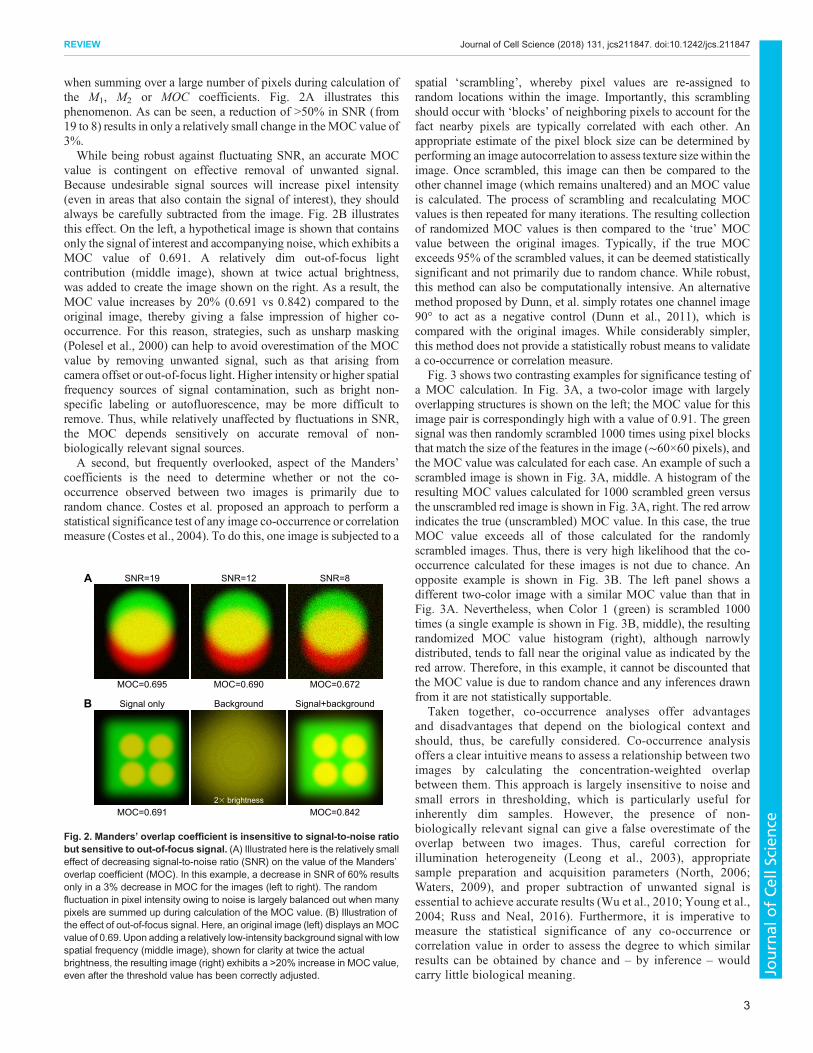
when summing over a large number of pixels during calculation ofthe M1, M2 or MOC coefficients. Fig. 2A illustrates thisphenomenon. As can be seen, a reduction of >50% in SNR (from19 to 8) results in only a relatively small change in theMOC value of3%.While being robust against fluctuating SNR, an accurate MOC

value is contingent on effective removal of unwanted signal.Because undesirable signal sources will increase pixel intensity(even in areas that also contain the signal of interest), they shouldalways be carefully subtracted from the image. Fig. 2B illustratesthis effect. On the left, a hypothetical image is shown that containsonly the signal of interest and accompanying noise, which exhibits aMOC value of 0.691. A relatively dim out-of-focus lightcontribution (middle image), shown at twice actual brightness,was added to create the image shown on the right. As a result, theMOC value increases by 20% (0.691 vs 0.842) compared to theoriginal image, thereby giving a false impression of higher co-occurrence. For this reason, strategies, such as unsharp masking(Polesel et al., 2000) can help to avoid overestimation of the MOCvalue by removing unwanted signal, such as that arising fromcamera offset or out-of-focus light. Higher intensity or higher spatialfrequency sources of signal contamination, such as bright non-specific labeling or autofluorescence, may be more difficult toremove. Thus, while relatively unaffected by fluctuations in SNR,the MOC depends sensitively on accurate removal of non-biologically relevant signal sources.A second, but frequently overlooked, aspect of the Manders’

coefficients is the need to determine whether or not the co-occurrence observed between two images is primarily due torandom chance. Costes et al. proposed an approach to perform astatistical significance test of any image co-occurrence or correlationmeasure (Costes et al., 2004). To do this, one image is subjected to a

spatial ‘scrambling’, whereby pixel values are re-assigned torandom locations within the image. Importantly, this scramblingshould occur with ‘blocks’ of neighboring pixels to account for thefact nearby pixels are typically correlated with each other. Anappropriate estimate of the pixel block size can be determined byperforming an image autocorrelation to assess texture sizewithin theimage. Once scrambled, this image can then be compared to theother channel image (which remains unaltered) and an MOC valueis calculated. The process of scrambling and recalculating MOCvalues is then repeated for many iterations. The resulting collectionof randomized MOC values is then compared to the ‘true’ MOCvalue between the original images. Typically, if the true MOCexceeds 95% of the scrambled values, it can be deemed statisticallysignificant and not primarily due to random chance. While robust,this method can also be computationally intensive. An alternativemethod proposed by Dunn, et al. simply rotates one channel image90° to act as a negative control (Dunn et al., 2011), which iscompared with the original images. While considerably simpler,this method does not provide a statistically robust means to validatea co-occurrence or correlation measure.

Fig. 3 shows two contrasting examples for significance testing ofa MOC calculation. In Fig. 3A, a two-color image with largelyoverlapping structures is shown on the left; the MOC value for thisimage pair is correspondingly high with a value of 0.91. The greensignal was then randomly scrambled 1000 times using pixel blocksthat match the size of the features in the image (∼60×60 pixels), andthe MOC value was calculated for each case. An example of such ascrambled image is shown in Fig. 3A, middle. A histogram of theresulting MOC values calculated for 1000 scrambled green versusthe unscrambled red image is shown in Fig. 3A, right. The red arrowindicates the true (unscrambled) MOC value. In this case, the trueMOC value exceeds all of those calculated for the randomlyscrambled images. Thus, there is very high likelihood that the co-occurrence calculated for these images is not due to chance. Anopposite example is shown in Fig. 3B. The left panel shows adifferent two-color image with a similar MOC value than that inFig. 3A. Nevertheless, when Color 1 (green) is scrambled 1000times (a single example is shown in Fig. 3B, middle), the resultingrandomized MOC value histogram (right), although narrowlydistributed, tends to fall near the original value as indicated by thered arrow. Therefore, in this example, it cannot be discounted thatthe MOC value is due to random chance and any inferences drawnfrom it are not statistically supportable.

Taken together, co-occurrence analyses offer advantagesand disadvantages that depend on the biological context andshould, thus, be carefully considered. Co-occurrence analysisoffers a clear intuitive means to assess a relationship between twoimages by calculating the concentration-weighted overlapbetween them. This approach is largely insensitive to noise andsmall errors in thresholding, which is particularly useful forinherently dim samples. However, the presence of non-biologically relevant signal can give a false overestimate of theoverlap between two images. Thus, careful correction forillumination heterogeneity (Leong et al., 2003), appropriatesample preparation and acquisition parameters (North, 2006;Waters, 2009), and proper subtraction of unwanted signal isessential to achieve accurate results (Wu et al., 2010; Young et al.,2004; Russ and Neal, 2016). Furthermore, it is imperative tomeasure the statistical significance of any co-occurrence orcorrelation value in order to assess the degree to which similarresults can be obtained by chance and – by inference – wouldcarry little biological meaning.

A

B

SNR=19

MOC=0.695

MOC=0.691

Signal only

SNR=12

MOC=0.690

Background

SNR=8

MOC=0.672

MOC=0.842

Signal+background

2� brightness

Fig. 2. Manders’ overlap coefficient is insensitive to signal-to-noise ratiobut sensitive to out-of-focus signal. (A) Illustrated here is the relatively smalleffect of decreasing signal-to-noise ratio (SNR) on the value of the Manders’overlap coefficient (MOC). In this example, a decrease in SNR of 60% resultsonly in a 3% decrease in MOC for the images (left to right). The randomfluctuation in pixel intensity owing to noise is largely balanced out when manypixels are summed up during calculation of the MOC value. (B) Illustration ofthe effect of out-of-focus signal. Here, an original image (left) displays an MOCvalue of 0.69. Upon adding a relatively low-intensity background signal with lowspatial frequency (middle image), shown for clarity at twice the actualbrightness, the resulting image (right) exhibits a >20% increase in MOC value,even after the threshold value has been correctly adjusted.

3

REVIEW Journal of Cell Science (2018) 131, jcs211847. doi:10.1242/jcs.211847

Journal

ofCe

llScience

In general, Manders’ coefficients are useful for assessing to whatextent a structure or molecule can be found in a particular location ororganelle. For example, it has been used to quantify the co-occurrence of a molecule of interest with mitochondria (Bravo et al.,2011; Seibler et al., 2011), the plasma membrane (Yeung et al.,2008; Spira et al., 2012) or the endoplasmic reticulum (Horner et al.,2011; Arruda et al., 2014). Importantly, however, Manders’approach does not signify that any predictable relationship existsbetween the intensities in one image and the corresponding valuesin the other. The MOC only expresses the degree to which twostructures spatially overlap, in an intensity-weighted manner. Itcannot positively indicate, for example, that areas of high intensityin one image correspond to low-intensity areas in the other and viceversa, which may be a sign of an important biological phenomenon.

Correlation: Pearson’s coefficientWhile the Manders’ overlap coefficients express the extent of co-occurrence between two images, correlation-based co-localizationanalyses are based on a different interpretation of co-localization. Inthis case, the guiding assumption states that, if two imaging targetsare functionally related, then their abundances will also bepredictably related to each other wherever they exist in the sameregion. This assumption is particularly relevant when probing twomolecules that are thought to bind to (or repulse) each other withinthe cell – even if such interactions may be rare. In other words,correlation methods measure the relationship between the signalintensities in one image and the corresponding values in another,not the degree to which the signals co-occur.Pearson’s correlation coefficient (PCC) is a common metric to

measure the predictability of this relationship (Pearson, 1896;Manders et al., 1993). In more mathematical terms, the PCC can bethought of as the covariance between the two images, normalized bythe product of their standard deviations:

PCC ¼Pn

i¼1ðxi � �xÞðyi � �yÞffiffiffiffiffiffiffiffiffiffiffiffiffiffiffiffiffiffiffiffiffiffiffiffiffiffiffiffiffiPni¼1 ðxi � �xÞ2

q ffiffiffiffiffiffiffiffiffiffiffiffiffiffiffiffiffiffiffiffiffiffiffiffiffiffiffiffiffiPni¼1 ðyi � �yÞ2

q ; ð6Þ

where xi and �x represent the ith pixel intensity and the averagepixel intensity (ignoring sub-threshold pixels), respectively, in thesegmented color 1 image. Likewise, yi and �y are the correspondingith and mean values for the color 2 image. The value of n representsthe total number of segmented pixels in both images. Recall that thevalue of n must be the same for both images since correlation

analysis should be performed on the intersection of the images inquestion.

In more conceptual terms, the PCC determines to what extent thesignal intensity variation in one image can be explained by thecorresponding variation in the other, assuming a linear relationship.Since the calculation of the PCC involves the difference of pixelintensity from the population mean, it can be either positive ornegative and can range from −1 to 1. The magnitude of the PCCgives a measure of the predictability of the relationship. Valuesclose to 1 or −1 indicate a near-perfect ability to infer a color 2intensity, given the corresponding color 1 intensity and vice versa.Values near zero indicate that there is little predictive value betweenthe images and that the two species being imaged do not have a clearcorrelation. The sign of the PCC indicates the ‘direction’ of therelationship between color 1 and color 2, with a positive signindicating that, when color 1 intensity increases, color 2 tends toincrease proportionally, pointing to a molecular attraction. Anegative sign implies the reverse, suggesting molecular repulsion.The ability to distinguish positive and negative correlation,therefore, represents a significant strength of the PCC coefficientover the Manders’ methods, owing to its ability to quantify bothpositive and negative associations.

Critical to the understanding of correlation-based image similaritymeasurements is the use of the scatterplot. Scatterplots are constructedby plotting the intensity value of each pixel in one image along the x-axis and on the y-axis the intensity value of the same pixel location inthe second image, thereby forminga bivariate histogram that describesthe relationship between the corresponding intensity values. It isimportant to note that a given region within a scatterplot does notnecessarily correspond to specific areas within the images, as thisrepresentation contains only intensity information.

Most importantly, a multi-color image may exhibit relatively highco-occurrence, while – at the same time – it can be poorly correlated,and vice versa. For example, analysis of the multicolor image shownin Fig. 4A results in relatively large Manders’ coefficients, withM1,M2 andMOC values of 0.81, 0.89 and 0.89, respectively. However,upon inspection of the corresponding scatterplot (Fig. 4B), apredictive relationship between the intensities of correspondinggreen and red pixels is not apparent, and calculation of the PCCconfirms this with a relatively low value of 0.11. Fig. 4C and Dillustrate a contrasting example. In this case, the M1, M2 and MOCvalues are found to be 0.13, 0.15 and 0.14, respectively, indicatinglittle co-occurrence. Nevertheless, the corresponding PCC value of

A

B

Fig. 3. Image randomization to test the statisticalsignificance of the Manders’ overlap coefficient. (A) Atrue multicolor image (left) that exhibits a Manders’ overlapcoefficient (MOC) value of 0.91. By using Costes’randomization method, the green-color image wasscrambled 1000 times in blocks whose size was determinedby autocorrelation. A single example of a randomized image(right). MOC was calculated for each of the scrambled greenimages and the original red-color image. The histogramshows the resulting values, in which the true (unscrambled)MOC value (red arrow) exceeds the randomized MOCvalues in all cases, indicating high statistical confidence inthe MOC. (B) A different multicolor image (left), with analmost identical MOC value to A (MOC=0.90). Costes’randomization method was applied to the green-channelimage as before. An example of a scrambled green image,overlaid with the original red image is shown (right). Theresulting MOC histogram shows that the true MOC value isnot consistently greater than the randomized values,suggesting the co-occurrence is mainly due to chance and,thus, has poor statistical significance.

4

REVIEW Journal of Cell Science (2018) 131, jcs211847. doi:10.1242/jcs.211847

Journal

ofCe

llScience

0.97 indicates an almost perfect correlation among the imageintersection. Therefore, although the data in Fig. 4C and D do notco-occur to a high degree, the intensity values are closely relatedwherever they overlap in the two images. Thus, the Manders’ andPearson’s coefficients can, in certain circumstances, give differentindications of image similarity. Although seemingly contradictory,such a result can provide powerful biological insight, as well asemphasizes the inherent differences between co-occurrence andcorrelation.The sensitivity of a PCC value to changing SNR and the addition

of unwanted low spatial frequency signal differs considerably fromco-occurrence approaches. To demonstrate this, Fig. 5A shows howthe PCC values for three green-red image pairs are affected byprogressively decreasing signal-to-noise ratio (SNR). This decreasein SNR is accompanied by a clear broadening of the correspondingscatter plots shown below each image pair, with an ∼35% reductionin PCC value. This behavior is in contrast to that of the Manders’coefficients, where relatively large changes in SNR have little effecton the MOC value (refer to Fig. 2A).Likewise, correlation and co-occurrence methods also respond

differently to unwanted low-frequency signal. Whereas the MOCrequires careful subtraction of such signals for accuratemeasurements (refer to Fig. 2B), the PCC is less sensitive to suchartefacts. This can be illustrated by simply adding a constant offsetto the images in Fig. 5A. Although this will shift the data points inthe scatterplot along the x- and y-axes, the predictability of theirrelationship will remain the same (ignoring saturated pixels).Therefore, a potential weakness of the PCC method lies in its

sensitivity to SNR. Decreasing SNR results in the relationship

between the pixel intensities of each image becoming less predictiveand increases the chances of an inadvertent inclusion of dimunwanted signal during threshold calculation. Imaging the samefield of view multiple times to measure noise characteristics canlessen the impact of low SNR on PCC value, but requires some apriori assumptions about the underlying relationship between theimages (Adler et al., 2008). To identify an optimal threshold valuefor correlation analysis, Costes et al. also proposed a means tosegment images on the basis of computing the PCC value across arange of threshold values (Costes et al., 2004). In this approach,continually decreasing thresholds for the two images are proposed,and the PCC value is calculated for pixels both above and belowthose threshold values. When the PCC value for the sub-thresholdpixels nears zero, an assumption is made that a suitablesegmentation of signal from background has been made.However, care must be taken when using Costes’ thresholdregression. If the signal of interest is not well correlated comparedto the background, there will not be a clear demarcation in the PCCvalues between the two. It is also important to note that Costes’significance testing scheme is equally applicable to correlationanalysis, as illustrated in the co-occurrence analysis in Fig. 3 (Costeset al., 2004). It should, therefore, always be performed to assess thereliability of an MOC or PCC result.

Correlation: Spearman’s coefficientThere are cases where PCC can give unexpected results. Thisincludes situations where the two images are well – but not linearly– correlated. In other words, the relationship between two imagesmay be very predictable but the scatterplot describing an imageintensity relationship is not well described by a straight line. In thesetypes of case, the PCC can underestimate the correlation betweenimages because the PCC can only approach its maximal magnitude(1 or −1) when the pixel intensity relationship is linear. However,Spearman’s rank correlation coefficient (SRCC) can address thisissue. In short, the SRCC is equivalent to the PCC, but is applied topixel intensity ranks rather than to the intensities themselves(Spearman, 1904). The conversion from pixel value to pixel rankproceeds such that the lowest above-threshold pixel intensity in theimage is given a value of 1, the next lowest value is assigned a rankof 2, and so on. In cases where multiple pixels have the sameintensity, that value is given an average rank. For example, if twopixels are tied for 3rd and 4th lowest value (rank 3–4), they are givenan ‘average’ rank of 3.5. The practical effect of this transformation isthat it linearizes the scatterplot from the two images, making thePearson’s analysis applicable to non-linear correlation.

Fig. 5B,C illustrates how the SRCC can be used to properlymeasure multicolor image correlation. In Fig. 5B, two almostidentical images are displayed (first two panels). The correspondingintensity scatterplot is displayed in the third and the ranked intensityscatterplot in the last panel. Note that both the intensity and rankedintensity scatterplots show a clear linear relationship, and the PCCand SRCC are both near unity. However, Fig. 5C illustrates theadvantage of SRCC over PCC. Here, although the color 1 image isidentical to that in Fig. 5B, the color 2 image has been altered so itproduces the intensity scatterplot shown in the third panel. This plotindicates a well-correlated but non-linear relationship between color1 and color 2. Despite the good predictability of the scatterplot, thePCC value is lower than expected (0.875) due to its non-linearity.However, by ranking the pixel intensity values, the relationshipbecomes linearized and the resulting SRCC value (0.989; last panel)does more accurately reflect the predictive relationship of theimages. Importantly, the SRCC is also useful for reducing the effect

A

C D

B

Fig. 4. Co-occurrence and correlation can occur independently of eachother. (A,B) The image shows an example of high co-occurrence (MOC=0.89)but with low correlation (PCC=0.11) (A). The low correlation can be clearlyseen in the corresponding intensity scatterplot (B), as there is no clearstatistical dependence between the corresponding pixels of each color image.(C) By contrast, the image shown here displays a relatively low co-occurrencebetween the red and green channels (MOC=0.14). (D) Nevertheless, whenonly the intersection of both color images is considered, the correspondingpixel intensities have a clear linear relationship, with a PCC value over theintersection of the red and green images almost equaling one. This serves toillustrate that correlation and co-occurrence are independent phenomena, asthey measure distinct behavior in an image pair. While co-occurrence gaugesthe overlap between signals in two images, correlation measures therelationship between those signals in overlapping areas.

5

REVIEW Journal of Cell Science (2018) 131, jcs211847. doi:10.1242/jcs.211847

Journal

ofCe

llScience

of pixel saturation as, in this case, the ranked value will generallydeviate less from the corresponding mean than the absolute intensityvalue.Unlike the Manders’ approach, correlation-based analyses do not

measure the extent to which one image overlaps with another.Indeed, high values of PCC or SRCC can occur even when thefractional co-occurrence is low (see Fig. 4). This can be especiallyapparent when two imaging targets are anti-correlated or when theyonly rarely interact. Correlation analysis simply measures how wellthe intensities in one image predict those in the other image, whensignal is present in the same pixel. This can be a powerful method tosuggest a functional relationship, such as – among many others –those shown for the assembly of endocytosis regulators (Teis et al.,

2008), association of focal adhesion components (Roca-Cusachset al., 2013; Carisey et al., 2013) or viral replication machineryassembly (Hsu et al., 2010).

Taken together, Figs 4 and 5 illustrate the requirements andlimitations of PCC or SRCC as a measure of co-localization.Further, these illustrations indicate the fundamental differencesbetween co-occurrence and correlation, with an eye towardsinferring the type of biological analysis that may be better suitedto one approach than another. For these correlation-based methodsto give meaningful results, the SNR in both images should bemaximized to the extent that is practical. As shown in Fig. 5, thePCC can fail to give an expected result if the correlation betweentwo images is non-linear. Interestingly, however, calculating the

A

B

PCC=0.998

Color 1 Color 2 Intensity scatter plot Ranked scatter plot

C

SRCC=0.997

PCC=0.875 SRCC=0.989

Fig. 5. The Pearson’s correlation coefficient is sensitive to both signal-to-noise ratio and scatterplot non-linearity. (A) Shown here is a series of threegreen and red image pairs whose signal-to-noise ratio (SNR) is progressively decreasing from 50 to 13 (scale not shown) from left via middle to right image. Thecorresponding scatterplots are shown below each image pair; they illustrate progressive broadening, and a decrease in the Pearson’s correlation coefficient(PCC) of ∼35%. (B) Two, almost identical, images shown in the green (left) and red (right) channel, and the corresponding intensity and ranked intensityscatterplots, both of which are linear. (C) The same green image as shown in B (left) compared to a different red image (right). This image pair exhibits a non-linearrelationship in their intensity scatterplot with a lower PCC value of 0.875. However, a ranked intensity scatterplot (see main text) recovers the linear relationship,with the resulting SRCC value almost equaling one (SRCC=0.989).

6

REVIEW Journal of Cell Science (2018) 131, jcs211847. doi:10.1242/jcs.211847

Journal

ofCe

llScience

SRCC for linearly correlated images still provides an accurate result.For these reasons, the SRCC should always be used in favor of thePCC. Fundamentally, however, both correlation and co-occurrencemeasurements yield different interpretations of co-localization. Yet,these interpretations can often be complementary.To further illustrate these considerations, Fig. 6 shows two

examples of biological associations. In A (top panel), a confocalimage of an U2OS cell reveals the distribution of epidermal growthfactor receptor (EGFR) (Herbst, 2004), tagged with GFP. Themiddle image shows Rab13 (Zerial and McBride, 2001) expressedas an mCherry-tagged fusion protein in the same cell. Fig. 6Bshows confocal images of a Ptk2 cell immunostained for bothtotal myosin (top panel) and phosphorylated myosin (middlepanel), respectively. The last image in A and B, each displays thecorresponding pixel intensity scatterplots for each of the proteinpairs. Appropriate signal threshold values for each image werecalculated by using Otsu’s method (Otsu, 1975). Then, theManders’, Pearson’s and Spearman’s coefficients were calculatedas described previously, and their results are summarized inFig. 6C.Qualitatively, the image pairs appear to have comparable levels of

similarity and the MOC values are, indeed, almost the same.However, the individual Manders’ coefficients reveal importantdifferences. Although almost all of the EGFR signal overlaps withthat of Rab13, not all Rab13 co-occurs with EGFR. This suggeststhat, although Rab13 may associate with EGFR, it may also beassociated with other molecules at different cellular locations. Totaland phosphorylated myosin, however, co-occur with each othernearly equally. The level of correlation between these two examplesis strikingly different, as suggested by their correspondingscatterplots. The PCC and SRCC values confirm this, with a two-fold difference in their value. The intersecting EGFR and Rab13concentrations predict each other relatively well, indicating aconcentration-dependent relationship between these molecules(Ioannou and McPherson, 2016). However, the overall abundanceof myosin does not predictably determine the concentration ofphosphorylated myosin (and vice versa), suggesting the presence ofother regulatory mechanisms (Goeckeler et al., 2000). This exampleillustrates the value to co-localization analysis in a holistic approachthat considers both overall and individual co-occurrence as well ascorrelation, in order to gain a broader range of biological insights.

Super-resolution imagingAs discussed initially, any image similarity measure is subject to theresolving power of the imaging system being used. Super-resolutionimaging circumvents the diffraction-limit and may offer detail that isotherwise unavailable. Techniques that improve resolution by ∼1.5to 2-fold, such as structured illumination microscopy (SIM)(Gustafsson et al., 2008), or image scanning microscopy and itsderivatives (Müller and Enderlein, 2010; York et al., 2013), offer thepossibility of increased accuracy when using pixel-based imagesimilarity measurements – as long as the interacting structures ofinterest both occur within in the same image pixels. Indeed, imagingtargets that appear co-localized under conventional imaging, may infact be well separated with even a modest improvement in resolution(Schermelleh et al., 2008). However, the near-molecular levelresolution of single-molecule localization (SML) techniques, suchas photo-activation and localization microscopy (PALM) (Betziget al., 2006) or stochastic optical reconstruction microscopy(STORM) (Rust et al., 2006), begin to reveal the effects of thePauli exclusion principle, which states that no two molecules canoccupy the same space at the same time.

A

C

B

Fig. 6. Interpreting co-occurrence and correlation analysis in twoexamples of biological data. (A) Confocal images of an U2OS cell that revealthe distribution of epidermal growth factor receptor (EGFR) (top) and Rab13(middle), expressed as GFP- and mCherry-tagged fusion proteins,respectively. The two-color overlay image is shown in the bottom image and thecorresponding pixel intensity scatterplot is shown underneath. (B) Confocalimages of a Ptk2 cell immunostained for total myosin (#3674, Cell Signaling)(top) and phosphorylated myosin (#922701, BioLegend) (middle), afterapplication of secondary antibodies conjugated to Alexa Fluor 488 and AlexaFluor 594 (Thermo Fisher), respectively. The corresponding two-color overlay isshown in the bottom image and the corresponding pixel intensity scatterplot isshown underneath. (C) Summary of the co-occurrence and correlationcoefficients, including Manders’ overlap (MOC), individual Manders’coefficients (M1 and M2), Pearson’s correlation coefficient (PCC) andSpearman’s rank correlation coefficients (SRCC). As can be seen, both imagepairs show similar levels of total overlap, with almost identical MOC values.However, the fractional overlap valuesM1 andM2 indicate important differencesbetween the two biological systems. Furthermore, the PCC and SRCC valuesalso indicate that, while EGFR and Rab13 have a clear concentrationrelationship, the abundance of phosphorylatedmysosin is not dependent on thetotal amount of mysosin, suggesting a secondary effector. Thus, carefulconsideration of both correlation and co-occurrencemetrics can reveal differentaspects of these biological systems.

7

REVIEW Journal of Cell Science (2018) 131, jcs211847. doi:10.1242/jcs.211847

Journal

ofCe

llScience

For SML techniques, spatial statistics have been utilized toquantitatively measure molecular associations without spatialoverlap (Coltharp et al., 2014; Lagache et al., 2015; Nicovichet al., 2017; Rossy et al., 2014; Georgieva et al., 2016; Malkuschet al., 2012). Malkusch et al. proposed a method termed coordinate-based co-localization (CBC) analysis. The procedure first calculatestwo functions,

Dxi;xðrÞ ¼Nxi;xðrÞ

Nxi;xðRmaxÞ �R2max

r2ð7Þ

and

Dxi;yðrÞ ¼Nxi;yðrÞ

Nxi;yðRmaxÞ �R2max

r2; ð8Þ

where Nxi;xðrÞ indicates the number of molecules of type x (or color1) that are found within a radius r surrounding a given singlelocalization, xi, of the same molecule type. Rmax refers to themaximum search radius, which should be larger than the expectedinteraction distance. In the second expression, Nxi;yðrÞ is definedanalogously, but counts the number of molecules of type y (or color2) within the same radius r and maximum distance Rmax. For each xi,an SRCC is then calculated between Nxi;xðrÞ and Nxi;yðrÞ. In thisway, a correlation value can be assigned to each molecule within theSML image. However, instead of a measure of intensity correlation,it reflects howwell two types of molecule are correlated in space. Byassigning each localization a CBC value, a ‘map’ can be constructedthat shows areas of both high and low spatial correlation within theimage.Another class of SML co-localization measures is based on

Ripley’s K-function (Ripley, 1977, 1976) and can serve as anensemble measure of interaction distance between two differentmolecules:

KijðrÞ ¼ A

NiNj

XNi

i¼1

XNj

j¼1

Iðdij , rÞwij

: ð9Þ

Here, A is the total imaging area (or volume in the case of 3D data),while Ni and Nj are the total number of localized molecules in eachimaging channel. I(dij<r) has a value of 1 if the distance between theith particle in channel one and the jth particle in channel two(denoted by dij) is less than r and zero otherwise. A correctionfactor, wij, is included to account for undercounting particles nearthe edge of the image (Haase, 1995). If two molecules are randomlydistributed with respect to each other, then Kij(r)=πr2. Thus, we candefine an L-function, such that

LijðrÞ ¼ KijðrÞ � pr2: ð10ÞFinding local maxima (or minima) in Lij(r) can, therefore, yieldcharacteristic interaction (or repulsion) distances (Kiskowski et al.,2009). A variant of Ripley’s K-function is termed pair-correlationfunction. Here, only the molecules contained within a ring withinner radius r and outer radius r+dr are included. Pair correlation ismore sensitive to local changes in molecule density around a givenlocalization, which can result in a more accurate measure ofcharacteristic interaction distance. However, it also depends on ahigh localization density within the image.Importantly, Ripley’s K-function (or pair correlation function)

and CBC can be used in tandem to gain complementaryinformation. CBC assigns a correlation value to each localizationin the image, thereby creating a map that can highlight areas of highor low association. Ripley’s K-function (and the related pair

correlation function), while only offering a global measure ofassociation, can provide a characteristic association distancebetween two different molecules that is missing in the CBCanalysis.

Conclusions and future perspectivesQuantitative image co-localization analyses, while utilized innumerous life science studies, represent a toolbox that is prone toflawed usage and misinterpretation. Contributing to this problem isthe fact that co-localization can be interpreted in at least two distinctways – co-occurrence or correlation. Both interpretations haveinherent, and often opposing, strengths and weaknesses. On onehand, measuring co-occurrence by using the Manders’ coefficientscan offer an intuitive accounting of the concentrated weightedoverlap between two imaging targets, with relative insensitivity toimaging noise. Yet, MOC values can be artefactually inflated byunwanted signal, such as out-of-focus light or endogenousfluorescence. On the other hand, correlation-based analysis offersa means to evaluate the intensity interdependence between imagesand, thus, is better able to distinguish both molecular attraction andrepulsion from random association. However, correlation measuressuch as PCC and SRCC work best when both images display a highSNR and are more sensitive to changes in threshold values.Importantly, Spearman’s rank correlation (Spearman, 1904) shouldalways be preferred over Pearson’s correlation (Pearson, 1896) toaccount for possible non-linear associations between images, and toguard against any pixel pair outliers, such as those occurring due toimage saturation. The statistical significance of any MCC, PCC orSRCC value should be assessed by Costes’ randomization approach(Costes et al., 2004) wherever possible.

Previous treatments of this subject have given recommendationson the appropriate approach based on image characteristics (Dunnet al., 2011; Bolte and Cordelieres, 2006) advocated for thesuperiority of correlation over co-occurrence (Adler and Parmryd,2010) or attempted to incorporate both concepts into a mergedmetric of overall co-localization (Zinchuk et al., 2013). We arguethat the specific biological question at hand should guide both theimage acquisition and analysis strategy. As illustrated in Figs 4 and6, co-occurrence and correlation can occur independently of eachother, and the extent of either phenomenon is largely determined bythe biological behavior being probed. Considering both types ofmetric can also yield complementary information.

In addition, the effect of so-called ‘global bias’ has not beenhistorically discussed in the context of image co-localization.Global bias refers to any external factor that can affect theinteraction between two molecules, apart from their affinity foreach other. Zaritsky and colleagues have proposed a powerfulmeans to separate local interactions from global relationships thatcan confound co-localization measurements (Zaritsky et al., 2017).Factors that can induce a global bias are numerous and can bebiological or non-biological, such as cell shape, cell cycle state,spatially correlated noise or offset in the detector, out-of-focussignal, or any combination thereof. For this reason, any imagingmodality that does not suppress out-of-focus light might lead toinaccurate results due to its inclusion of signal from above andbelow the focal plane. Confocal and TIRF microscopy are,therefore, better imaging methodologies for such analyses, as theyconfine excitation or detection to within the depth of field of theobjective lens (Conchello and Lichtman, 2005; Schneckenburger,2005). Furthermore, the advent of super-resolution techniques can,in principle, offer greater fidelity when inferring molecularinteractions. However, structures that might spatially overlap

8

REVIEW Journal of Cell Science (2018) 131, jcs211847. doi:10.1242/jcs.211847

Journal

ofCe

llScience

when interrogated with conventional modalities can, in fact, bewell-separated when using subject to super-resolution microscopy.In general, as achievable resolution improves, the intersection oftwo multi-channel images necessarily approaches zero and pixel-based similarity measures are rendered obsolete, favoring spatialstatistical approaches instead (Nicovich et al., 2017; Coltharp et al.,2014; Lagache et al., 2015). But, while the ultra-high resolutionattainable in PALM and STORM imaging can be attractive, thesemethods typically preclude imaging dynamic samples. Further, thepreferred means to analyze these data is computationally intensive.Thus, careful consideration must be paid to the underlyingbiological behavior being investigated to select the optimalimaging and analysis method. Any co-localization measurementsare most meaningful when expressed as relative changes. Evaluationof a coefficient value relative to stringent controls (both positive andnegative) and/or over time will significantly strengthen its ability todraw meaningful biological conclusions. In summary, thecomplexity of co-localization analysis demands carefulconsideration to determine the best approach to answer a givenbiological question. Furthermore, as imaging technology continuesto improve, strategies for measuring biomolecular associations willbe required to evolve concomitantly.

AcknowledgementsWe thank Satya Khuon, Maria Ioannou and Damien Alcor (HHMI Janelia ResearchCampus) for assistance in preparing and imaging biological samples.

Competing interestsThe authors declare no competing or financial interests.

FundingThe authors gratefully acknowledge support from the Advanced Imaging Center atJanelia Research Campus, a facility jointly funded by the Gordon and Betty MooreFoundation and the Howard Hughes Medical Institute.

ReferencesAbbe, E. (1873). Beitrage zur Theorie des Mikroskops und der mikroskopischenWahrnehmung. Arch. Fur Mikrosk. Anat. 9, 413-418.

Adler, J. and Parmryd, I. (2010). Quantifying colocalization by correlation: thePearson correlation coefficient is superior to the Mander’s overlap coefficient.Cytometry A. 77A, 733-742.

Adler, J., Pagakis, S. N. and Parmryd I. (2008). Replicate-based noise correctedcorrelation for accuratemeasurements of colocalization. J. Microsc. 230, 121-133.

Arruda, A. P., Pers, B. M., Parlakgul, G., Guney, E., Inouye, K. and Hotamisligil,G. S. (2014). Chronic enrichment of hepatic endoplasmic reticulum-mitochondriacontact leads to mitochondrial dysfunction in obesity. Nat. Med. 20, 1427-1435.

Betzig, E., Patterson, G. H., Sougrat, R., Lindwasser, O. W., Olenych, S.,Bonifacino, J. S., Davidson, M. W., Lippincott-Schwartz, J. and Hess, H. F.(2006). Imaging intracellular fluorescent proteins at nanometer resolution.Science 313, 1642-1645.

Bolte, S. and Cordelieres, F. P. (2006). A guided tour into subcellular colocalizationanalysis in light microscopy. J. Microsc. 224, 213-232.

Bravo, R., Vicencio, J. M., Parra, V., Troncoso, R., Munoz, J. P., Bui, M., Quiroga,C., Rodriguez, A. E., Verdejo, H. E., Ferreira, J. et al. (2011). Increased ER–mitochondrial coupling promotes mitochondrial respiration and bioenergeticsduring early phases of ER stress. J. Cell Sci. 124, 2143.

Carisey, A., Tsang, R., Greiner, A. M., Nijenhuis, N., Heath, N., Nazgiewicz, A.,Kemkemer, R., Derby, B., Spatz, J. and Ballestrem, C. (2013). Vinculinregulates the recruitment and release of core focal adhesion proteins in a force-dependent manner. Curr. Biol. 23, 271-281.

Chudakov, D. M., Matz, M. V., Lukyanov, S. and Lukyanov, K. A. (2010).Fluorescent proteins and their applications in imaging living cells and tissues.Physiol. Rev. 90, 1103.

Coltharp, C., Yang, X. and Xiao, J. (2014). Quantitative analysis of single-moleculesuperresolution images. Curr. Opin. Struct. Biol. 28, 112-121.

Conchello, J.-A. and Lichtman, J. W. (2005). Optical sectioning microscopy. Nat.Methods 2, 920-931.

Costes, S. V., Daelemans, D., Cho, E. H., Dobbin, Z., Pavlakis, G. and Lockett, S.(2004). Automatic and quantitative measurement of protein-protein colocalizationin live cells. Biophys. J. 86, 3993-4003.

Dickinson, M. E., Bearman, G., Tille, S., Lansford, R. and Fraser, S. E. (2002).Multi-spectral imaging and linear unmixing add a whole new dimension to laserscanning fluorescence microscopy. BioTechniques 31, 1272-1278.

Dunn, K. W., Kamocka, M. M. and McDonald, J. H. (2011). A practical guide toevaluating colocalization in biological microscopy. Am. J. Physiol. Cell Physiol.300, C723-C742.

Georgieva, M., Cattoni, D. I., Fiche, J.-B., Mutin, T., Chamousset, D. andNollmann, M. (2016). Nanometer resolved single-molecule colocalization ofnuclear factors by two-color super resolution microscopy imaging. Methods 105,44-55.

Glasbey, C. A. (1993). An analysis of histogram-based thresholding algorithms.CVGIP Graph. Models Image Process. 55, 532-537.

Goeckeler, Z. M., Masaracchia, R. A., Zeng, Q., Chew, T.-L., Gallagher, P. andWysolmerski, R. B. (2000). Phosphorylation of myosin light chain kinase by p21-activated kinase PAK2. J. Biol. Chem. 275, 18366-18374.

Grimm, J. B., English, B. P., Chen, J., Slaughter, J. P., Zhang, Z., Revyakin, A.,Patel, R., Macklin, J. J., Normanno, D., Singer, R. H. et al. (2015). A generalmethod to improve fluorophores for live-cell and single-molecule microscopy. Nat.Methods 12, 244-250.

Gustafsson, M. G. L., Shao, L., Carlton, P. M., Wang, C. J. R., Golubovskaya,I. N., Cande, W. Z., Agard, D. A. and Sedat, J. W. (2008). Three-dimensionalresolution doubling in wide-field fluorescence microscopy by structuredillumination. Biophys. J. 94, 4957-4970.

Haase, P. (1995). Spatial pattern analysis in ecology based on Ripley’s K-function:Introduction and methods of edge correction. J. Veg. Sci. 6, 575-582.

Helmuth, J. A., Paul, G. and Sbalzarini, I. F. (2010). Beyond co-localization:inferring spatial interactions between sub-cellular structures from microscopyimages. BMC Bioinformatics 11, 372.

Herbst, R. S. (2004). Review of epidermal growth factor receptor biology.Int. J. Radiat. Oncol. 59, S21-S26.

Horner, S. M., Liu, H. M., Park, H. S., Briley, J. and Gale, M. (2011). Mitochondrial-associated endoplasmic reticulum membranes (MAM) form innate immunesynapses and are targeted by hepatitis C virus. Proc. Natl. Acad. Sci. USA 108,14590-14595.

Hsu, N.-Y., Ilnytska, O., Belov, G., Santiana, M., Chen, Y.-H., Takvorian, P. M.,Pau, C., van der Schaar, H., Kaushik-Basu, N., Balla, T. et al. (2010). Viralreorganization of the secretory pathway generates distinct organelles for RNAreplication. Cell 141, 799-811.

Ioannou, M. S. andMcPherson, P. S. (2016). Regulation of cancer cell behavior bythe small GTPase Rab13. J. Biol. Chem. 291, 9929-9937.

Kiskowski, M. A., Hancock, J. F. and Kenworthy, A. K. (2009). On the use ofRipley’s K-function and its derivatives to analyze domain size. Biophys. J. 97,1095-1103.

Lagache, T., Sauvonnet, N., Danglot, L. and Olivo-Marin, J.-C. (2015). Statisticalanalysis of molecule colocalization in bioimaging. Cytometry A 87, 568-579.

Lange, S., Katayama, Y., Schmid, M., Burkacky, O., Brauchle, C., Lamb, D. C.and Jansen, R.-P. (2008). Simultaneous transport of different localized mRNAspecies revealed by live-cell imaging. Traffic 9, 1256-1267.

Leong, F. J. W.-M., Brady, M. and McGee, J. O. (2003). Correction of unevenillumination (vignetting) in digital microscopy images. J. Clin. Pathol. 56, 619-621.

Malkusch, S., Endesfelder, U., Mondry, J., Gelleri, M., Verveer, P. J. andHeilemann, M. (2012). Coordinate-based colocalization analysis of single-molecule localization microscopy data. Histochem. Cell Biol. 137, 1-10.

Manders, E. M. M., Verbeek, F. J. and Aten, J. A. (1993). Measurement of co-localization of objects in dual-colour confocal images. J. Microsc. 169, 375-382.

Muller, C. B. and Enderlein, J. (2010). Image scanning microscopy. Phys. Rev.Lett. 104, 198101.

Nakagawa, Y. and Rosenfeld, A. (1979). Some experiments on variablethresholding. Pattern Recognit. 11, 191-204.

Nakamura, J. (Ed.). (2017). Image sensors and signal processing for digital stillcameras. CRC Press, Boca Raton, FL, USA.

Nicovich, P. R., Owen, D. M. and Gaus, K. (2017). Turning single-moleculelocalization microscopy into a quantitative bioanalytical tool. Nat. Protoc. 12,453-460.

North, A. J. (2006). Seeing is believing? A beginners’ guide to practical pitfalls inimage acquisition. J. Cell Biol. 172, 9-18.

Otsu, N. (1975). A threshold selection method from gray-level histograms.Automatica 11, 23-27.

Pearson, K. (1896). Mathematical contributions to the theory of evolution. III.regression, heredity, and panmixia. Philos. Trans. R. Soc. Lond. Math. Phys. Eng.Sci. 187, 253-318.

Piston, D. W. and Kremers, G.-J. (2007). Fluorescent protein FRET: the good, thebad and the ugly. Trends Biochem. Sci. 32, 407-414.

Polesel, A., Ramponi, G. and Mathews, V. J. (2000). Image enhancement viaadaptive unsharp masking. IEEE Trans. Image Process. 9, 505-510.

Pun, T. (1980). A newmethod for grey-level picture thresholding using the entropy ofthe histogram. Signal Process. 2, 223-237.

Ripley, B. (1976). The second-order analysis of stationary point processes. J. Appl.Probab. 13, 255-266.

9

REVIEW Journal of Cell Science (2018) 131, jcs211847. doi:10.1242/jcs.211847

Journal

ofCe

llScience

Ripley, B. D. (1977). Modelling spatial patterns. J. R. Stat. Soc. Ser. B Methodol 39,172-212.

Roca-Cusachs, P., del Rio, A., Puklin-Faucher, E., Gauthier, N. C., Biais, N. andSheetz, M. P. (2013). Integrin-dependent force transmission to the extracellularmatrix by α-actinin triggers adhesion maturation. Proc. Natl. Acad. Sci. 110,E1361-E1370.

Rossy, J., Cohen, E., Gaus, K. and Owen, D. M. (2014). Method for co-clusteranalysis in multichannel single-molecule localisation data. Histochem. Cell Biol.141, 605-612.

Russ, J. C. (2016). The Image Processing Handbook. (6th Ed.). CRC Press, BocaRaton, FL, USA.

Russ, J. C. and Russ, J. C. (1987). Automatic discrimination of features in grey-scale images. J. Microsc. 148, 263-277.

Rust, M. J., Bates, M. and Zhuang, X. (2006). Sub-diffraction-limit imaging bystochastic optical reconstruction microscopy (STORM).Nat. Methods 3, 793-796.

Schermelleh, L., Carlton, P. M., Haase, S., Shao, L., Winoto, L., Kner, P., Burke,B., Cardoso, M. C., Agard, D. A., Gustafsson, M. G. L. et al. (2008).Subdiffraction multicolor imaging of the nuclear periphery with 3D structuredillumination microscopy. Science 320, 1332.

Schneckenburger, H. (2005). Total internal reflection fluorescence microscopy:technical innovations and novel applications. Anal. Biotechnol. 16, 13-18.

Seibler, P., Graziotto, J., Jeong, H., Simunovic, F., Klein, C. and Krainc, D.(2011). Mitochondrial park in recruitment is impaired in neurons derived frommutant PINK1 induced pluripotent stem cells. J. Neurosci. 31, 5970.

Sezgin, M. and Sankur, B. (2004). Survey over image thresholding techniques andquantitative performance evaluation. 13, 146-165.

Shaner, N. C., Steinbach, P. A. and Tsien, R. Y. (2005). A guide to choosingfluorescent proteins. Nat. Methods 2, 905-909.

Spearman, C. (1904). The proof and measurement of association between twothings. Am. J. Psychol. 15, 72-101.

Spira, F., Mueller, N. S., Beck, G., von Olshausen, P., Beig, J. and Wedlich-Soldner, R. (2012). Patchwork organization of the yeast plasma membrane intonumerous coexisting domains. Nat. Cell Biol. 14, 640-648.

Stelzer, E. H. K. (1998). Contrast, resolution, pixelation, dynamic range and signal-to-noise ratio: fundamental limits to resolution in fluorescence light microscopy.J. Microsc. 189, 15-24.

Sternberg, S. R. (1983). Biomedical image processing. Computer 16, 22-34.

Teis, D., Saksena, S. and Emr, S. D. (2008). Ordered assembly of the ESCRT-IIIcomplex on endosomes is required to sequester cargo during MVB formation.Dev. Cell 15, 578-589.

Truong, K. and Ikura, M. (2001). The use of FRET imaging microscopy to detectprotein–protein interactions and protein conformational changes in vivo. Curr.Opin. Struct. Biol. 11, 573-578.

Waters, J. C. (2009). Accuracy and precision in quantitative fluorescencemicroscopy. J. Cell Biol. 185, 1135-1148.

Wu, Q., Merchant, F. and Castleman, K. (2010). Microscope Image Processing.Academic Press, Burlington, MA, USA.

Wysocki, L. M. and Lavis, L. D. (2011). Advances in the chemistry of smallmolecule fluorescent probes. Mol. Imaging 15, 752-759.

Yeung, T., Gilbert, G. E., Shi, J., Silvius, J., Kapus, A. and Grinstein, S. (2008).Membrane phosphatidylserine regulates surface charge and protein localization.Science 319, 210.

York, A. G., Chandris, P., Nogare, D. D., Head, J., Wawrzusin, P., Fischer, R. S.,Chitnis, A. and Shroff, H. (2013). Instant super-resolution imaging in live cellsand embryos via analog image processing. Nat. Methods 10, 1122-1126.

Young, I., Gerbrands, J. J. and Van Vliet, L. (1998). Fundamentals Of ImageProcessing. Delft University of Technology, Delft, The Netherlands.

Zaritsky, A., Obolski, U., Gan, Z., Reis, C. R., Kadlecova, Z., Du, Y., Schmid, S. L.andDanuser, G. (2017). Decoupling global biases and local interactions betweencell biological variables. eLife 6, e22323.

Zerial, M. and McBride, H. (2001). Rab proteins as membrane organizers. Nat.Rev. Mol. Cell Biol. 2, 107.

Zinchuk, V. and Grossenbacher-Zinchuk, O. (2008). Quantitative colocalizationanalysis of confocal fluorescencemicroscopy images. InCurrent Protocols in CellBiology. 4-16.

Zinchuk, V., Zinchuk, O. andOkada, T. (2007). Quantitative colocalization analysisof multicolor confocal immunofluorescence microscopy images: pushing pixels toexplore biological phenomena. Acta Histochem. Cytochem 40, 101-111.

Zinchuk, V., Wu, Y. and Grossenbacher-Zinchuk, O. (2013). Bridging the gapbetween qualitative and quantitative colocalization results in fluorescencemicroscopy studies. Sci. Rep. 3, 1365.

Zitova, B. and Flusser, J. (2003). Image registration methods: a survey. Image Vis.Comput. 21, 977-1000.

10

REVIEW Journal of Cell Science (2018) 131, jcs211847. doi:10.1242/jcs.211847

Journal

ofCe

llScience