
Image Analysis on Symmetric Positive Definite...
120
Image Analysis on Symmetric Positive Definite Manifolds Azadeh Alavi Master of IT-Advanced, Bachelor of Applied Mathematics A thesis submitted for the degree of Doctor of Philosophy at The University of Queensland in 2014 School of Information Technology and Electrical Engineering
-
Upload
nguyentruc -
Category
Documents
-
view
223 -
download
0
Transcript of Image Analysis on Symmetric Positive Definite...
Image Analysis on Symmetric Positive Definite Manifolds
Azadeh Alavi
Master of IT-Advanced, Bachelor of Applied Mathematics
A thesis submitted for the degree of Doctor of Philosophy at
The University of Queensland in 2014
School of Information Technology and Electrical Engineering

Abstract
Over the last two decades, the research community has witnessed extensive
research growth in the field of analysing and understanding scenes. Auto-
matic scene analysis can support many critical applications, from person re-
identification as an advanced security tool, to real-time action classification
as an assistive technology for disabled patients. However, building effective
systems is still a challenge due to the presence of occlusion, varying illumi-
nation, varying pose and other factors encountered in the practical environ-
ment.
To deal with the real world environment, which is naturally not free from
noise, a recent trend in computer vision is to represent a given image through
a covariance matrix of a set of extracted features. Covariance matrices are
robust to noise and are well known to be compact and informative feature
descriptors. Non-singular covariance matrices are naturally symmetric pos-
itive definite (SPD) matrices which form connected Riemannian manifolds.
As such, their underlying distance and similarity functions might not be ac-
curately defined in Euclidean space, and consequently the Riemannian ge-
ometry needs to be considered in order to solve scene analysing tasks. The
traditional methods of analysing such manifolds require embedding them in
Euclidean spaces, a process which can be interpreted as warping the fea-
ture space. However, embedding manifolds is not free from drawbacks and
it can lead to limitations, as the manifold structure may not be accurately
preserved.
In this work we propose three methods for analysing SPD matrices on
Riemannian manifolds that unlike traditional methods respect the underlying
structure of a given image, while considering the computational complexity
of the learning algorithm. While all three methods offer strong solutions
for the task of image analysis over SPD manifolds that outperform state-of-
the-art methods, each of them tends to tackle one vision application better
than the rest. This is owed to the existing differences between each vision
application. Although all of these vision tasks can be categorised as a image
classification problem, each application offers unique challenges, such as very
limited training data, strong pose variation etc. To be more specific, the
first proposed method outperforms the rest of the proposed methods in face
recognition; the extension of the second method performs very well in the
task of person re-identification; and the last proposed method outperforms
other two in the task of texture recognition.
This work addresses the challenge of analysing SPD manifolds using the
below proposed methods:
1. Graph-Embedding Discriminant Analysis
2. Relational Divergence Based Classification
3. Random Projections
The first method proposes to embed Riemannian manifolds into Repro-
ducing Kernel Hilbert Spaces (RKHS) and then tackle the problem of dis-
criminant analysis on the Hilbert space. To achieve an efficient machinery,
we present a graph-based local discriminant analysis that utilises within-class
and between-class similarity graphs to characterise intra-class compactness
and inter-class separability. Experiments on face recognition, texture classifi-
cation and person re-identification indicate that the proposed method obtains
marked improvement in discrimination accuracy in comparison to several
state-of-the-art methods.
The second proposed method suggests direct classification on the Man-
ifold by presenting each SPD matrix through its similarity vector with the
number of other SPD matrices. In addition, to speed up the process, the
proposed method employs the recently introduced Stein divergence. Classifi-
cation problems on manifolds are then effectively converted into the problem
of finding appropriate machinery over the space of similarities. Experiments
on face recognition, texture classification and person re-identification show
that in comparison to well-known methods, the proposed approach obtains
a significant improvement in image classification, while also being several
orders of magnitude faster.
The third proposed algorithm proposes to project SPD matrices using a
set of random projection hyperplanes over an RKHS into a random projec-
tion space, which leads to representing each matrix as a vector of projec-
tion coefficients. Experiments on face recognition, person re-identification

and texture classification show that the proposed approach, in comparison to
well-known methods, obtains a significant improvement in image classifica-
tion, while also being relatively faster.
Experiments and comparative evaluations on standard datasets from a
variety of image analysis applications suggest that the three proposed algo-
rithms obtain considerably better results (both qualitatively and quantita-
tively) than other well-known techniques available in the literature. While
all three proposed methods have been designed to work for scenes analysis,
the experiment result suggest that based on the nature of the given appli-
cation (i.e., the number of points in the training set), one of the proposed
algorithms might be favoured over the rest.

Declaration by Author
This thesis is composed of my original work, and contains no material pre-
viously published or written by another person except where due reference
has been made in the text. I have clearly stated the contribution by others to
jointly-authored works that I have included in my thesis.
I have clearly stated the contribution of others to my thesis as a whole, in-
cluding statistical assistance, survey design, data analysis, significant techni-
cal procedures, professional editorial advice, and any other original research
work used or reported in my thesis. The content of my thesis is the result
of work I have carried out since the commencement of my research higher
degree candidature and does not include a substantial part of work that has
been submitted to qualify for the award of any other degree or diploma in
any university or other tertiary institution. I have clearly stated which parts
of my thesis, if any, have been submitted to qualify for another award.
I acknowledge that an electronic copy of my thesis must be lodged with the
University Library and, subject to the General Award Rules of The University
of Queensland, immediately made available for research and study in accor-
dance with the Copyright Act 1968.
I acknowledge that copyright of all material contained in my thesis resides
with the copyright holder(s) of that material. Where appropriate I have ob-
tained copyright permission from the copyright holder to reproduce material
in this thesis.

Contributions by Others to the Thesis
The work contained in this thesis was carried out by the author under the
guidance and supervision of her advisors, Prof. Brian C. Lovell and Dr. Con-
rad Sanderson. Part of the work contained in this thesis was carried out by
the author in collaboration and discussion with Dr. Mehrtash T. Harandi and
Dr. Arnold Wiliem.
Statement of Parts of the Thesis Submitted to Qualify for the Award of
Another Degree
None

Acknowledgements
I wish to express my sincere gratitude to my supervisors Prof. Brian C.
Lovell and Dr. Conrad Sanderson for their guidance, encouragement, and
support throughout my PhD studies. The drive and work-discipline of both
Prof. Lovell and Dr. Sanderson have been exemplary, and I sincerely hope
that I have picked up some of their drive and discipline along the way. I am
grateful to Dr. Mehrtash Harandi and Dr. Arnold Wiliem for their valuable
inputs and suggestions, which are reflected in this work. I would also like to
knowledge professor Peter Hobson and express my gratitude for his support.
Many thanks are due to my friends and colleagues for their encouragement
and support during all of these years. I would like to sincerely acknowledge
the support of The University of Queensland and NICTA by awarding scholar-
ships and providing necessary resources to undertake this work. I also wish
to acknowledge our lab’s external research partners, Queensland Rail and
Port of Brisbane for permitting us to access live surveillance feeds, which
aided in developing better algorithms, presented in this work. In addition,
I would like to acknowledge Sullivan Nicolaides Pathology, Australia, and
the Australian Research Council (ARC) Linkage Projects Grant LP130100230
who have partly funded this research. Finally, I am indebted to my family, in
particular to my parents, Fatemeh Kouchmeshki and Abdolrahman Alavi, and
my husband Hossein Akhoundi for their love, support and understanding.

Keywords
computer vision, pattern recognition, machine learning, differentiable mani-
folds, symmetric positive definite manifolds, riemannian manifolds
Australian and New Zealand Standard Research Classifications (ANZSRC)
ANZSRC code: 080104, Computer Vision, 40%
ANZSRC code: 080106, Image Processing, 30%
ANZSRC code: 010401, Applied Statistics, 30%
Fields of Research (FoR) Classification
FoR code: 0801, Artificial Intelligence and Image Processing, 70%
FoR code: 0104, Statistics, 30%
Contents
1 Introduction 22
1.0.1 Matrix Manifold . . . . . . . . . . . . . . . . . . . . . 23
1.1 Goals and Challenges . . . . . . . . . . . . . . . . . . . . . . . 25
1.2 Contributions . . . . . . . . . . . . . . . . . . . . . . . . . . . 27
1.2.1 Graph-Embedding Discriminant Analysis on Rieman-
nian Manifolds for Visual Recognition . . . . . . . . . 27
1.2.2 Relational Divergence Based Classification on Rieman-
nian Manifolds . . . . . . . . . . . . . . . . . . . . . . 28
1.2.3 Random Projections on Manifolds of Symmetric Posi-
tive Definite Matrices . . . . . . . . . . . . . . . . . . . 28
1.3 Thesis Outline . . . . . . . . . . . . . . . . . . . . . . . . . . . 29
1.3.1 Comprehensive Literature Review . . . . . . . . . . . . 30
2 Background theory 32
2.1 Non-Euclidean Geometry . . . . . . . . . . . . . . . . . . . . . 32
2.2 Differentiable Manifolds . . . . . . . . . . . . . . . . . . . . . 34
2.3 Riemannian Geometry . . . . . . . . . . . . . . . . . . . . . . 36
2.3.1 Tangent Space . . . . . . . . . . . . . . . . . . . . . . 37
2.3.2 Riemannian Metrics . . . . . . . . . . . . . . . . . . . 39
2.3.3 Types of Riemannian Manifolds . . . . . . . . . . . . . 41
2.4 Symmetric Positive Definite Manifolds . . . . . . . . . . . . . 43
2.4.1 Stein Divergence . . . . . . . . . . . . . . . . . . . . . 45
3 Graph-Embedding Discriminant Analysis on Riemannian Manifolds
for Visual Recognition 47
3.1 Overview . . . . . . . . . . . . . . . . . . . . . . . . . . . . . 47
3.2 Introduction . . . . . . . . . . . . . . . . . . . . . . . . . . . . 48
3.3 Kernel Analysis on Riemannian Manifolds . . . . . . . . . . . 49
3.3.1 Background . . . . . . . . . . . . . . . . . . . . . . . . 49
3.3.2 Graph Embedding Discriminant Analysis on Rieman-
nian Manifolds . . . . . . . . . . . . . . . . . . . . . . 51
3.3.3 Classification . . . . . . . . . . . . . . . . . . . . . . . 54
3.4 Experiments . . . . . . . . . . . . . . . . . . . . . . . . . . . . 55
3.4.1 Experiments on SPD Manifolds . . . . . . . . . . . . . 55
4 Relational Divergence Based Classification on Riemannian Mani-
folds 62
4.1 Relational Divergence Based Classification . . . . . . . . . . . 63
4.1.1 Overview . . . . . . . . . . . . . . . . . . . . . . . . . 63
4.1.2 Introduction . . . . . . . . . . . . . . . . . . . . . . . 64
4.1.3 Relational Divergence Classification . . . . . . . . . . 65
4.1.4 Experiments and Discussion . . . . . . . . . . . . . . . 67
4.1.5 Texture Classification . . . . . . . . . . . . . . . . . . . 68
4.1.6 Face Recognition . . . . . . . . . . . . . . . . . . . . . 70
4.1.7 Person Re-identification . . . . . . . . . . . . . . . . . 70
4.2 RDC for Person Re-identification . . . . . . . . . . . . . . . . 71
4.2.1 Overview . . . . . . . . . . . . . . . . . . . . . . . . . 71
4.2.2 Introduction . . . . . . . . . . . . . . . . . . . . . . . 72
4.2.3 Previous Work . . . . . . . . . . . . . . . . . . . . . . 74
4.2.4 Proposed approach . . . . . . . . . . . . . . . . . . . . 76
4.2.5 Similarity Vectors and Discriminative Mapping . . . . 78
4.2.6 Experiments and Discussion . . . . . . . . . . . . . . . 80
4.2.7 iLIDS Dataset . . . . . . . . . . . . . . . . . . . . . . . 80
4.2.8 ETHZ Dataset . . . . . . . . . . . . . . . . . . . . . . . 81
5 Random Projections on Manifolds of Symmetric Positive Definite
Matrices for Image Classification 84
5.1 Overview . . . . . . . . . . . . . . . . . . . . . . . . . . . . . 84
5.2 Introduction . . . . . . . . . . . . . . . . . . . . . . . . . . . . 85
5.3 Random Projection on RKHS . . . . . . . . . . . . . . . . . . 86
5.3.1 Synthetic Data . . . . . . . . . . . . . . . . . . . . . . 89
5.4 Experiments and Discussion . . . . . . . . . . . . . . . . . . . 92
5.4.1 Person Re-Identification . . . . . . . . . . . . . . . . . 93
5.4.2 Random Projection Space Discriminability . . . . . . . 94
5.4.3 Comparison with Recent Methods . . . . . . . . . . . . 97
6 Conclusion 100
6.1 Graph-Embedding Discriminant Analysis . . . . . . . . . . . . 101
6.1.1 Future work . . . . . . . . . . . . . . . . . . . . . . . . 101
6.2 Relational Divergence Based Classification . . . . . . . . . . . 102
6.2.1 Future work . . . . . . . . . . . . . . . . . . . . . . . . 102
6.3 Random Projection . . . . . . . . . . . . . . . . . . . . . . . . 102
6.3.1 Future work . . . . . . . . . . . . . . . . . . . . . . . . 103
6.4 Combining the proposed methods . . . . . . . . . . . . . . . . 103
6.4.1 Future work . . . . . . . . . . . . . . . . . . . . . . . . 104
Appendix 105
Codes 107
Bibliography 110
List of Figures
1.1 Examples from the VIPeR person re-identification dataset [GBT07a] . . . 23
2.1 φ maps some point of M to some point of Rn. . . . . . . . . . . . . . 35
2.2 φ maps each point of U and χ maps each point of V to some point of Rn.
The image demonstrates how more than one chart might be required to
cover all the points of M . . . . . . . . . . . . . . . . . . . . . . . 35
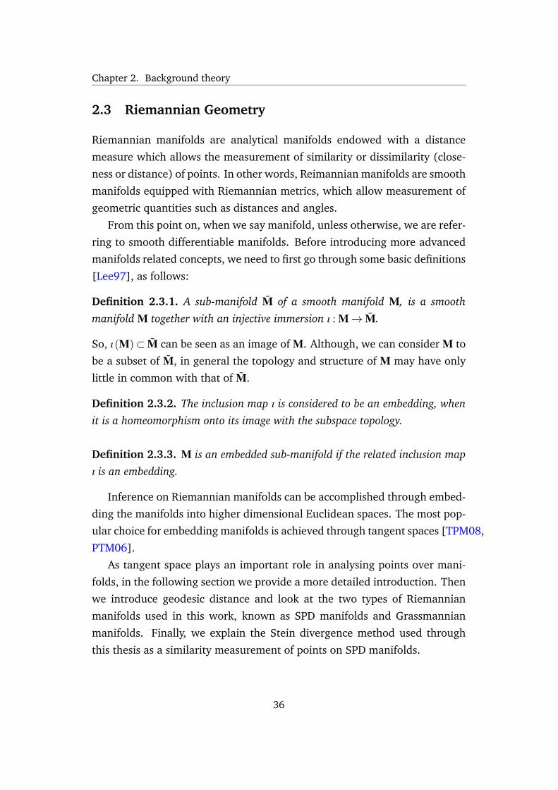
2.3 Relations between tangent spaces, tangent vectors, and geodesics. P1 and
P2 are points on the manifold, while TP1 and TP2 are tangent spaces at these
points [TVC08]. . . . . . . . . . . . . . . . . . . . . . . . . . . . 37
3.1 A conceptual illustration of the proposed approach. (a) Actions can be
modelled as points on the manifold M by linear subspaces. In this fig-
ure, two types of actions (”kicking” and ”swinging”) are shown. Having a
proper geodesic distance between the points on the manifold, it is possible
to convert the action recognition problem into a point to point classifica-
tion problem. (b) By having a kernel in hand, points on the manifold can
be mapped into an optimised RKHS where not only certain local properties
have been retained but also the discriminatory power between classes has
been increased. . . . . . . . . . . . . . . . . . . . . . . . . . . . 49
3.2 Examples of closely-cropped faces from the FERET ‘b’ subset. . . . . . . 56
3.3 Samples of Brodatz texture dataset [RH99]. . . . . . . . . . . . . . . 57
3.4 Performance on the Brodatz texture dataset [RH99] for Tensor Sparse Cod-
ing (TSC) [SBMP10] and the proposed RGDA approach. The black bars
indicate standard deviation. . . . . . . . . . . . . . . . . . . . . . 58
3.5 Examples of pedestrians in the ETHZ dataset. . . . . . . . . . . . . . 58
3.6 Performance on Sequence 1, 2, and 3 of the ETHZ dataset (top, middle and
bottom panels, respectively), in terms of Cumulative Matching Character-
istic curves. The proposed RGDA method is compared with Histogram Plus
Epitome (HPE) [BCP+10], and Symmetry-Driven Accumulation of Local
Features (SDALF) [FBP+10]. . . . . . . . . . . . . . . . . . . . . . 61
4.1 Performance on the Brodatz texture dataset [RH99] for LogE-SR [GIK10,
YHL+10], Tensor Sparse Coding (TSC) [SBMP10], Riemannian Locality
Preserving Projection (RLPP) [HSWL12] and the proposed RDC method. 68
4.2 Performance comparison on Sequence 1 (top) and 2 (bottom) of the ETHZ
dataset [SD09], in terms of Cumulative Matching Characteristic curves.
The proposed RDC method is compared with Riemannian Locality Preserv-
ing Projection (RLPP) [HSWL12], Histogram Plus Epitome (HPE) [BCP+10],
Symmetry-Driven Accumulation of Local Features (SDALF) [FBP+10] and
Partial Least Squares (PLS) [SD09]. . . . . . . . . . . . . . . . . . . 69
4.3 Examples of challenges in person re-identification, where each column con-
tains images of the same person from two separate camera views. Chal-
lenges include pose changes, occlusions of body parts, low resolution and
illumination variations. . . . . . . . . . . . . . . . . . . . . . . . 72
4.4 Performance on the iLIDS dataset [ZGX09] for N=3, using the proposed
RDC method, the direct Stein method, SDALF [FBP+10], context based
method [ZGX09]. HPE results for N=3 were not provided in [BCP+10]. . 81
4.5 Performance on the ETHZ dataset [SD09] for N = 10, using Sequences 1 to
3 (top to bottom). Results are shown for the proposed RDC method, direct
Stein method, HPE [BCP+10], PLS [SD09] and SDALF [FBP+10]. . . . . 83
5.1 The process of transferring points on SPD Manifold into Random Projection
Space. . . . . . . . . . . . . . . . . . . . . . . . . . . . . . . . 89
5.2 The above graphs show the sensitivity of the random projection space dis-
criminability to the number of selected data points for generating the ran-
dom hyperplanes, as well as the effect of adding synthetic data points for
improving space discriminability. The graphs compare the performance
of ROSE and ROSES on 5c (top) and 5m (bottom) sets of the BRODATZ
texture recognition dataset respectively. . . . . . . . . . . . . . . . . 96
List of Tables
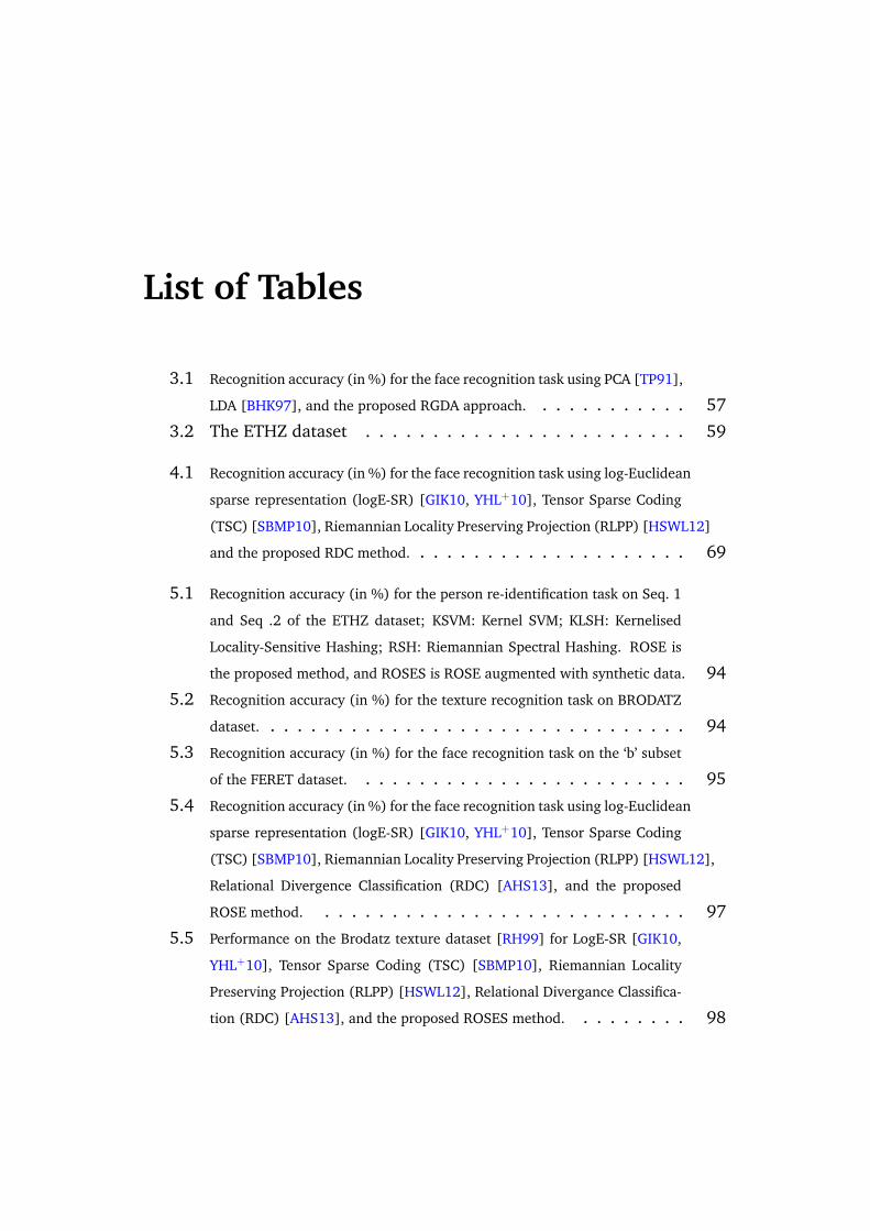
3.1 Recognition accuracy (in %) for the face recognition task using PCA [TP91],
LDA [BHK97], and the proposed RGDA approach. . . . . . . . . . . . 57
3.2 The ETHZ dataset . . . . . . . . . . . . . . . . . . . . . . . . 59
4.1 Recognition accuracy (in %) for the face recognition task using log-Euclidean
sparse representation (logE-SR) [GIK10, YHL+10], Tensor Sparse Coding
(TSC) [SBMP10], Riemannian Locality Preserving Projection (RLPP) [HSWL12]
and the proposed RDC method. . . . . . . . . . . . . . . . . . . . . 69
5.1 Recognition accuracy (in %) for the person re-identification task on Seq. 1
and Seq .2 of the ETHZ dataset; KSVM: Kernel SVM; KLSH: Kernelised
Locality-Sensitive Hashing; RSH: Riemannian Spectral Hashing. ROSE is
the proposed method, and ROSES is ROSE augmented with synthetic data. 94
5.2 Recognition accuracy (in %) for the texture recognition task on BRODATZ
dataset. . . . . . . . . . . . . . . . . . . . . . . . . . . . . . . . 94
5.3 Recognition accuracy (in %) for the face recognition task on the ‘b’ subset
of the FERET dataset. . . . . . . . . . . . . . . . . . . . . . . . . 95
5.4 Recognition accuracy (in %) for the face recognition task using log-Euclidean
sparse representation (logE-SR) [GIK10, YHL+10], Tensor Sparse Coding
(TSC) [SBMP10], Riemannian Locality Preserving Projection (RLPP) [HSWL12],
Relational Divergence Classification (RDC) [AHS13], and the proposed
ROSE method. . . . . . . . . . . . . . . . . . . . . . . . . . . . 97
5.5 Performance on the Brodatz texture dataset [RH99] for LogE-SR [GIK10,
YHL+10], Tensor Sparse Coding (TSC) [SBMP10], Riemannian Locality
Preserving Projection (RLPP) [HSWL12], Relational Divergance Classifica-
tion (RDC) [AHS13], and the proposed ROSES method. . . . . . . . . 98

5.6 Recognition accuracy (in %) for the person re-identification task on Seq.1
and Seq.2 of the ETHZ dataset. HPE: Histogram Plus Epitome [BCP+10];
SDALF: Symmetry-Driven Accumulation of Local Features [FBP+10]; RLPP:
Riemannian Locality Preserving Projection [HSWL12]; RDC: Relational Di-
vergence Classification [AHS13]. . . . . . . . . . . . . . . . . . . . 98
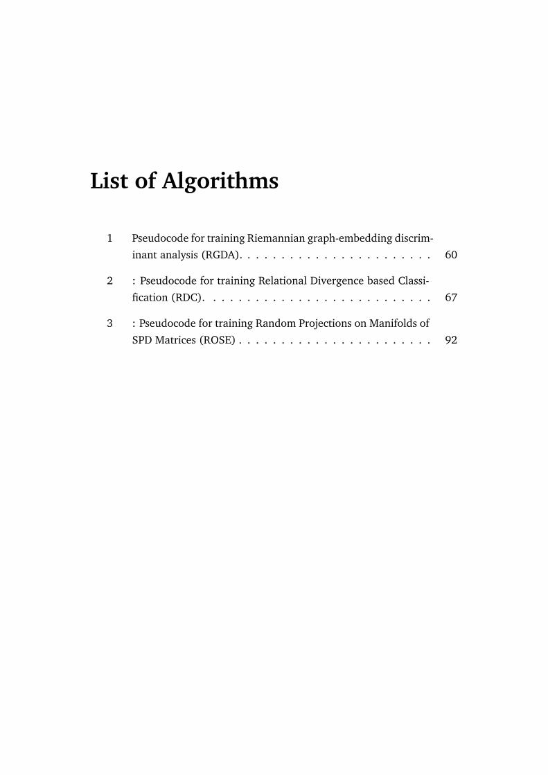
List of Algorithms
1 Pseudocode for training Riemannian graph-embedding discrim-
inant analysis (RGDA). . . . . . . . . . . . . . . . . . . . . . . 60
2 : Pseudocode for training Relational Divergence based Classi-
fication (RDC). . . . . . . . . . . . . . . . . . . . . . . . . . . 67
3 : Pseudocode for training Random Projections on Manifolds of
SPD Matrices (ROSE) . . . . . . . . . . . . . . . . . . . . . . . 92
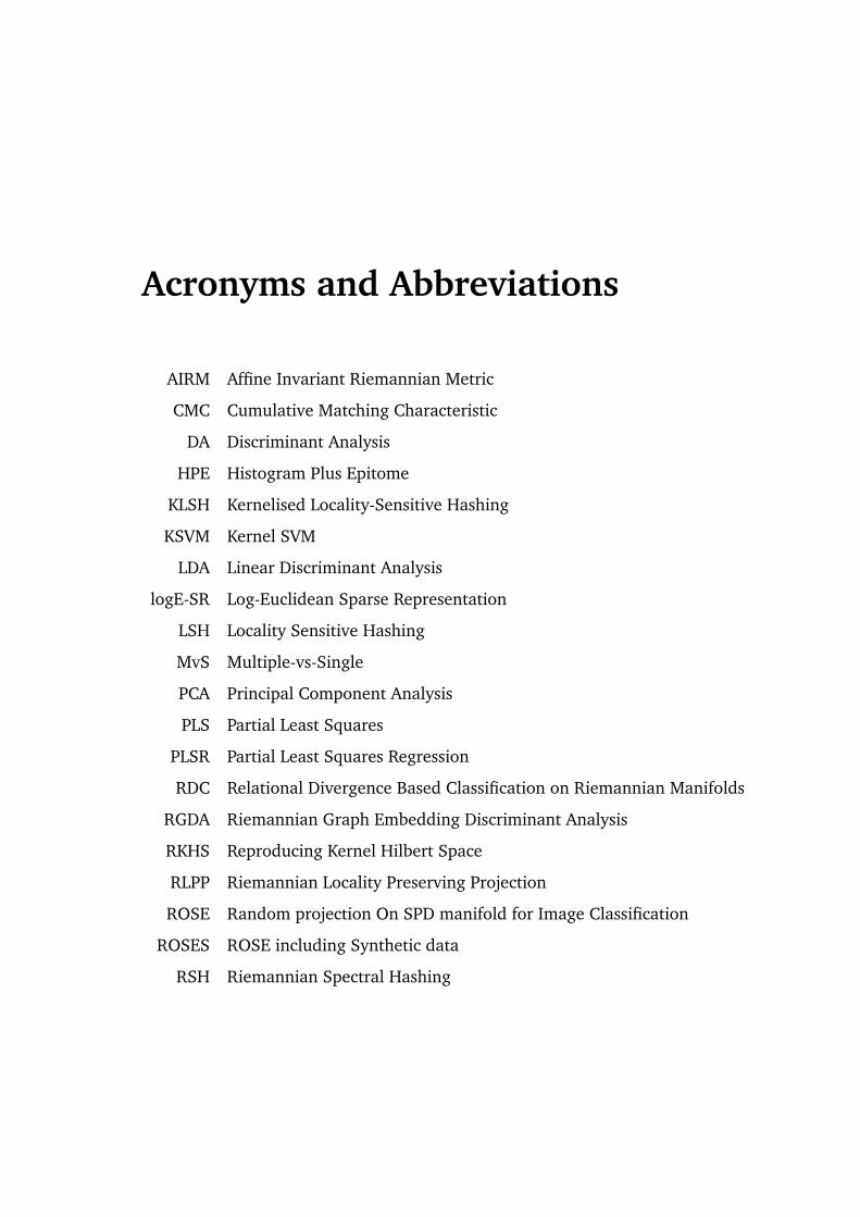
Acronyms and Abbreviations
AIRM Affine Invariant Riemannian Metric
CMC Cumulative Matching Characteristic
DA Discriminant Analysis
HPE Histogram Plus Epitome
KLSH Kernelised Locality-Sensitive Hashing
KSVM Kernel SVM
LDA Linear Discriminant Analysis
logE-SR Log-Euclidean Sparse Representation
LSH Locality Sensitive Hashing
MvS Multiple-vs-Single
PCA Principal Component Analysis
PLS Partial Least Squares
PLSR Partial Least Squares Regression
RDC Relational Divergence Based Classification on Riemannian Manifolds
RGDA Riemannian Graph Embedding Discriminant Analysis
RKHS Reproducing Kernel Hilbert Space
RLPP Riemannian Locality Preserving Projection
ROSE Random projection On SPD manifold for Image Classification
ROSES ROSE including Synthetic data
RSH Riemannian Spectral Hashing

SCM Sparsity-based Collaborative Model
SDALF Symmetry-Driven Accumulation of Local Features
SPD Symmetric Positive Definite
SR Sparse Representation
STEL Structural Element
SvS Single-vs-Single
SVD Singular Value Decomposition
SVM Support Vector Machine
TCCA Tensor Canonical Correlation Analysis
TSC Tensor Sparse Coding
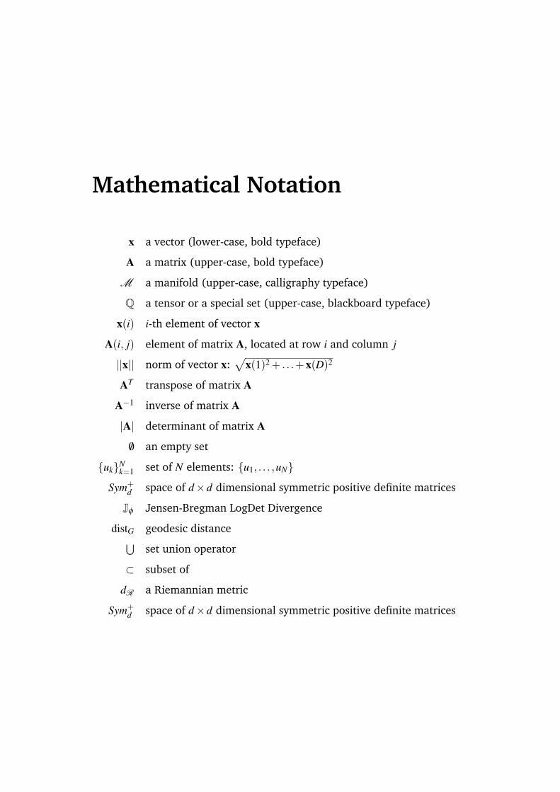
Mathematical Notation
x a vector (lower-case, bold typeface)
A a matrix (upper-case, bold typeface)
M a manifold (upper-case, calligraphy typeface)
Q a tensor or a special set (upper-case, blackboard typeface)
x(i) i-th element of vector x
A(i, j) element of matrix A, located at row i and column j
||x|| norm of vector x:√
x(1)2 + . . .+x(D)2
AT transpose of matrix A
A−1 inverse of matrix A
|A| determinant of matrix A
/0 an empty set
ukNk=1 set of N elements: u1, . . . ,uN
Sym+d space of d×d dimensional symmetric positive definite matrices
Jφ Jensen-Bregman LogDet Divergence
distG geodesic distance⋃set union operator
⊂ subset of
dR a Riemannian metric
Sym+d space of d×d dimensional symmetric positive definite matrices

Chapter 1
Introduction
Computer vision is a science that aims to design artificial visual machinery
that can analyse and interpret scenes information. It can be applied in vari-
ety of applications from security monitoring to enhancing medical diagnoses.
Some of the applications for scenes analysis are face recognition, cell classi-
fication, autonomous robotics, etc [CT10, JA10, YF08, FGR05]. Some exam-
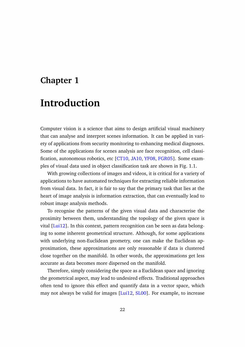
ples of visual data used in object classification task are shown in Fig. 1.1.
With growing collections of images and videos, it is critical for a variety of
applications to have automated techniques for extracting reliable information
from visual data. In fact, it is fair to say that the primary task that lies at the
heart of image analysis is information extraction, that can eventually lead to
robust image analysis methods.
To recognise the patterns of the given visual data and characterise the
proximity between them, understanding the topology of the given space is
vital [Lui12]. In this context, pattern recognition can be seen as data belong-
ing to some inherent geometrical structure. Although, for some applications
with underlying non-Euclidean geometry, one can make the Euclidean ap-
proximation, these approximations are only reasonable if data is clustered
close together on the manifold. In other words, the approximations get less
accurate as data becomes more dispersed on the manifold.
Therefore, simply considering the space as a Euclidean space and ignoring
the geometrical aspect, may lead to undesired effects. Traditional approaches
often tend to ignore this effect and quantify data in a vector space, which
may not always be valid for images [Lui12, SL00]. For example, to increase
22
Chapter 1. Introduction
Figure 1.1: Examples from the VIPeR person re-identification dataset [GBT07a]
robustness against noise, it is popular to present an image as a covariance of
a selected feature vectors such as colour, gradient and filter responses. The
covariance matrices belong to the space of d× d symmetric positive definite
matrices which forms a cone in the space of matrices, thus is not a vector
space [PFA06, TPM06a].
1.0.1 Matrix Manifold
To ensure that the underlying structure of the image is respected, manifold
learning techniques such as ISOmetric Mapping (ISOMAP) [TDSL00] and Lo-
cal Linear Embedding (LLE) [RS00] were introduced. These methods gener-
ally use a large amount of densely sampled training data to learn a mapping
from the ambient space to the intrinsic space; so that the projection of the
points is distance invariant.
If the underlying geometric structure of the data is already known, an-
other geometrical method can be employed which does not necessarily re-
quire the large amount of training data. The method suggests representing
images in an underlying parametrised space. This school of thought gives rise
23
Chapter 1. Introduction
to the representation of a matrix manifold [Lui12]. While manifold learning
techniques tend to learn a manifold through training data, matrix manifolds
methods derive from the properties of differential geometry. To be more
specific, a matrix manifold uses algebraic operations to characterise the id-
iosyncratic aspects of the geometry of the data in some parameter space; in
fact, image data are often described as the orbit of elements under the matrix
manifolds action (i.e., rotation group) [Lui12].
The concept of matrix manifolds dates back to the 19th century [Jam99].
Since then, they have gained more attention in the mathematics, physics, and
other scientific communities. Moreover, matrix manifolds enable the devel-
opment of similarity metrics, expressions for probability distributions, means
and covariances which can be useful for designing nearest neighbour and
Bayesian classifiers, support vector machines, and clustering and tracking
algorithms.
Matrix manifolds also naturally arise in computer vision as they enable the
representation of many types of image and video features in non-Euclidean
spaces [Che12]. Furthermore, matrix manifolds provide tools for design-
ing classifiers such as nearest neighbour and support vector machine by pro-
viding the means for the development of similarity metrics, expressions for
probability distributions, means and covariances [Che12]. This is still a very
popular research area and constitutes one of the challenging aspects of recog-
nising and classifying visual data.
In this research we focus on addressing the scenes analysis challenge
through matrix manifolds. To be more specific, in the domain of differen-
tiable manifolds we use the special class of Riemannian Manifolds known as
Symmetric Positive Definite (SPD) manifolds for analysing visual data.
24
Chapter 1. Introduction
1.1 Goals and Challenges
The work in this thesis proposes three approaches for analysing images over
Symmetric Positive Definite (SPD) manifolds which improves the performance
of major computer vision tasks that numerous image analysis applications are
confronted with.
Furthermore, the algorithms are designed to respect the underlying struc-
ture of the images with a view to achieve real-time performance. These three
approaches are:
1. Graph-Embedding Discriminant Analysis on Riemannian Manifolds for
Visual Recognition
2. Relational Divergence Based Classification on Riemannian Manifolds
3. Random Projections on Manifolds of Symmetric Positive Definite Matri-
ces
All three approaches are destined in a way to avoid the use of tangent
space by either mapping the data points into a Kernel Space or directly using
the similarity vectors over SPD manifolds. In the following, we will give a
brief description of the three proposed solutions.
As mentioned earlier, visual recognition is a fundamental task in a wide
range of computer vision applications such as security surveillance, person
re-identification and human-computer interaction. The general idea is to
improve the image classification system enabling reliable work in practical
environments containing pose and illumination variations, misalignment and
other varying conditions.
To this end, we contend that covariance matrices of the extracted image
features are the best means to model the images since they are able to pro-
vide compact and informative feature description that can accommodate the
above mentioned challenges. Non-singular covariance matrices are naturally
in the form of SPD matrices which form connected Riemannian manifolds
when endowed with a Riemannian metric over tangent spaces. Thereafter,
exploiting the non-Euclidean and curved geometry of manifolds is vital to
compare the SPD matrices without violating the underlying structure of the
matrices.
25

Chapter 1. Introduction
To increase the accuracy and speed of the inference on the SPD manifolds,
we proposed three approaches:
First approach developed a graph-based local discriminant analysis to em-
bed the SPD manifold into a Reproducing Kernel Hilbert space (RKHS) with
the intra-class compactness as well as inter-class separability.
The second approach employs the Stein Divergence dissimilarity measure-
ment to calculate the similarity vectors representing each SPD matrix.
The final approach employs Random Projection over RKHS and improves
the performance of image classification.
26
Chapter 1. Introduction
1.2 Contributions
Our main goal is to improve image classification on SPD manifolds without
violating the underlying structure of the manifold, while keeping the algo-
rithm computationally relatively inexpensive. In addition, our approaches
can be employed for any image analysis task.
In this thesis we propose three solutions for analysing images on SPD
manifolds with respect to the underlying structure
• Employing Graph-Embedding Discriminant Analysis on Riemannian Man-
ifolds for Visual Recognition
• Relational Divergence Based Classification on Riemannian Manifolds
• Random Projections on Manifolds of Symmetric Positive Definite Matri-
ces
Besides providing state-of-the-art algorithms to address these three tasks,
we made a series of contributions in terms of novel representation and clas-
sification approaches which could prove useful in alternative applications.
Below we enumerate our contributions per task. Note that our purpose
here is to give a brief overview of the contributions; further explanation of
the topics will be given later in the chapters attributed to each of the three
tasks.
1.2.1 Graph-Embedding Discriminant Analysis on Riemannian Mani-folds for Visual Recognition
• Tackles the problem of Discriminant Analysis (DA) on Riemannian man-
ifolds through RKHS space
• Proposes a graph-based local DA that utilises both within-class and between-
class similarity graphs to characterise intra-class compactness and inter-
class separability, respectively
27
Chapter 1. Introduction
1.2.2 Relational Divergence Based Classification on Riemannian Mani-folds
• Introduces a new way of analysing Riemannian manifolds where em-
bedding into Euclidean spaces or RKHS is not required
• Creates similarity vectors and discriminative mapping for final classifi-
cation
• The classification task on manifolds is then converted into a task in the
space of similarity vectors,
1.2.3 Random Projections on Manifolds of Symmetric Positive DefiniteMatrices
• Offers a novel approach for analysing SPD matrices which combines the
main advantage of tangent space approaches with the discriminatory
power provided by kernel space methods
• Embeds SPD manifold points into RKHS via the Stein Divergence Kernel
[Sra12a].
• Generates random projection hyperplanes in RKHS and project the em-
bedded points via the method proposed in [KG09].
• The classification task on manifolds is then converted into a task in the
Euclidean space
28
Chapter 1. Introduction
1.3 Thesis Outline
The rest of this thesis is comprised of four major parts. Chapter 2 provides
an overview of the relevant mathematical terms and theoretical aspects used
in this work. Chapter 3, Chapter 4 and Chapter 5 present our proposed solu-
tions targeting image analysis task on Symmetric Positive Definite manifolds
with respect to the underlying geometrical structure (i.e., without the aid of
tangent spaces). The above three chapters represent independent solutions
and include their own literature review and proposed algorithms. Our con-
cluding remarks and possible future directions are presented in Chapter 6.
Chapters 3 to 6 are summarised below:
• Chapter 2: Background Theory.
This chapter provides an overview of the relevant theory used in this
work. It starts with defining and describing Riemannian geometry fol-
lowed by a description of a tangent space. The curved shape of the
manifolds and the effect of the curvature on computing dissimilarity
between points is then explained. Finally, the Stein Divergence which
is employed in this thesis to calculate the dissimilarity between points
over Symmetric Positive Definite manifolds is explained in detail.
• Chapter 3: Graph-Embedding Discriminant Analysis on Riemannian
Manifolds for Visual Recognition. This chapter shows how discrimi-
nant analysis can be reformulated on non-Euclidean spaces, namely the
SPD manifolds. Inference on manifold spaces can be achieved by em-
bedding the manifolds in higher dimensional Euclidean spaces, which
can be considered as flattening the manifolds. In this work we pro-
pose to tackle the problem of Discriminant Analysis (DA) on Rieman-
nian manifolds through RKHS space and propose a graph-based local
DA that utilises both within-class and between-class similarity graphs to
characterise intra-class compactness and inter-class separability, respec-
tively.
• Chapter 4: Relational Divergence Based Classification on Rieman-
nian Manifolds. In this chapter we proposed to represent Riemannian
29
Chapter 1. Introduction
points through their similarities to a set of reference points on the man-
ifold, with the aid of the recently proposed Stein divergence, which
is a symmetrised version of Bregman matrix divergence. Classification
problems on manifolds are then effectively converted into the problem
of finding appropriate machinery over the space of similarities, which
can be tackled by conventional Euclidean learning methods such as lin-
ear discriminant analysis. This is then followed by expanding the work
to explicitly address the person re-identification task.
• Chapter 5: Random Projections on Manifolds of Symmetric Positive
Definite Matrices. This chapter presents a novel solution which em-
beds the data points into a random projection space by first generating
random hyperplanes in RKHS and then projecting the data in RKHS into
the random projection space.
• Chapter 6: Conclusion. This chapter summarises the contributions of
this thesis and enumerates new avenues and improvements for future
research.
1.3.1 Comprehensive Literature Review
As this work covers several distinct yet related solutions, each proposed
method has its own literature review. The overall literature review is com-
prised of:
• The entire chapter 2, which covers relevant background theory neces-
sary to build a solution based on Riemannian Manifolds (or to be more
specific Symmetric Positive Definite Manifolds).
• Section 3.2, which covers a literature review of the state-of-the-art stud-
ies that utilised non-Euclidean geometry (mainly focusing on Rieman-
nian Manifolds) to address several computer vision problems.
• Section 4.1.2, which covers popular choices for embedding Riemannian
manifolds and other proposed alternative solutions for analysing images
on Riemann manifolds.
30

Chapter 1. Introduction
• Section 4.2.2, which introduces the person re-identification task and its
main terminology, and is followed by Section 4.2.3 which goes through
literature review of the popular algorithms that target this area.
• Section 5.2, which presents a survey of state-of-the-art approaches for
mapping manifold points to Hilbert spaces, thereby enabling the use of
existing Euclidean-based learning algorithms.
31
Chapter 2
Background theory
This chapter introduces the required mathematical concepts and technical
background to provide a foundation for the rest of this work. First, we ex-
plain the concept of differentiable manifolds and introduce necessary defi-
nitions required in order to understand the rest of this thesis. Riemannian
geometry is then explained which is followed by introducing tangent space,
and then Riemannian metrics. Two types of Riemannian manifolds used in
this work known as Grassmannian Manifolds (chapter 3) and Symmetric Pos-
itive Definite (SPD) Manifolds(chapter 3, 4 and 5), are then introduced. The
distance function on such manifolds is subsequently introduced, followed by
the concept of Tangent Space. Then, as the main topic of interest of this
thesis is SPD manifolds, from this stage on, our main focus is to detail the
related SPD manifold concepts.
2.1 Non-Euclidean Geometry
Recently, several studies have utilised non-Euclidean geometry to address
several computer vision problems including object tracking [HLL+ss], charac-
terising the diffusion of water molecules as in diffusion tensor imaging [Pen06],
face recognition [PYL08, SBMP10], human re-identification [BCBTss], tex-
ture classification [HSWL12], pedestrian detection [TPM08] and action recog-
nition [OLDss, YHL+10].
In computer vision and machine learning disciplines, the trace of covari-
ance and kernel matrices can be seen in many ways. One notable example is
32
Chapter 2. Background theory
the covariance descriptor introduced by Tuzel et al. [TPM06b]. A covariance
descriptor is a structured representation and comes with several advantages
over traditional descriptors. A single covariance matrix extracted from a re-
gion (2D regions in images or 3D in videos) is usually enough to match the
region in different views and poses.
Furthermore, the covariance matrix proposes a natural way of fusing mul-
tiple features which might be correlated. The diagonal entries of the co-
variance matrix represent the variance of each feature and the non-diagonal
entries represent the covariances. The noise corrupting individual samples
are largely filtered out with an average filter during covariance computation.
Nevertheless, the space of covariance/correlation/kernel matrices (more gen-
erally symmetric positive definite matrices) is not Euclidean; it is a Rieman-
nian manifold of negative curvature.
Several studies show that better performance can be achieved when the
geometry of the Riemannian spaces is considered to its uttermost level [HL08,
TPM08, SM09, Lui12, HSSL11, TVSC11]. Exploiting the geometry of space
is especially important in the computer vision discipline since the notion of
Euclidean space is not well supported for high-dimensional vision data (c.f.,
think how inaccurate distances could be on a sphere when the geometry is
not considered).
33
Chapter 2. Background theory
2.2 Differentiable Manifolds
Generally speaking, employing the theory of differentiable manifolds enables
one to extend the applications, concepts and results of the calculus on Rn
spaces to sets that do not possess the structure of a normed vector space
[DC11]. Based on this definition one can absorb that many applications of
computer vision involve recognition of patterns from data which lie on such
manifolds [TVC08].
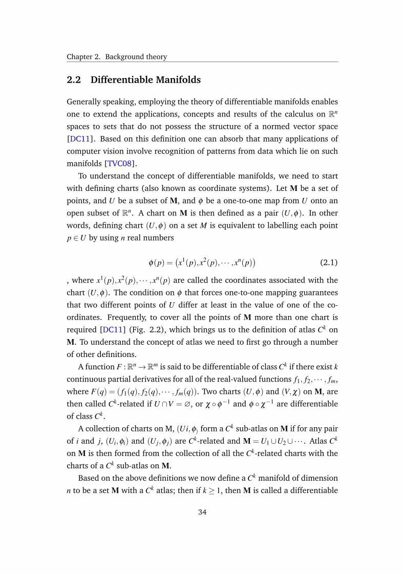
To understand the concept of differentiable manifolds, we need to start
with defining charts (also known as coordinate systems). Let M be a set of
points, and U be a subset of M, and φ be a one-to-one map from U onto an
open subset of Rn. A chart on M is then defined as a pair (U,φ). In other
words, defining chart (U,φ) on a set M is equivalent to labelling each point
p ∈U by using n real numbers
φ(p) =(x1(p),x2(p), · · · ,xn(p)
)(2.1)
, where x1(p),x2(p), · · · ,xn(p) are called the coordinates associated with the
chart (U,φ). The condition on φ that forces one-to-one mapping guarantees
that two different points of U differ at least in the value of one of the co-
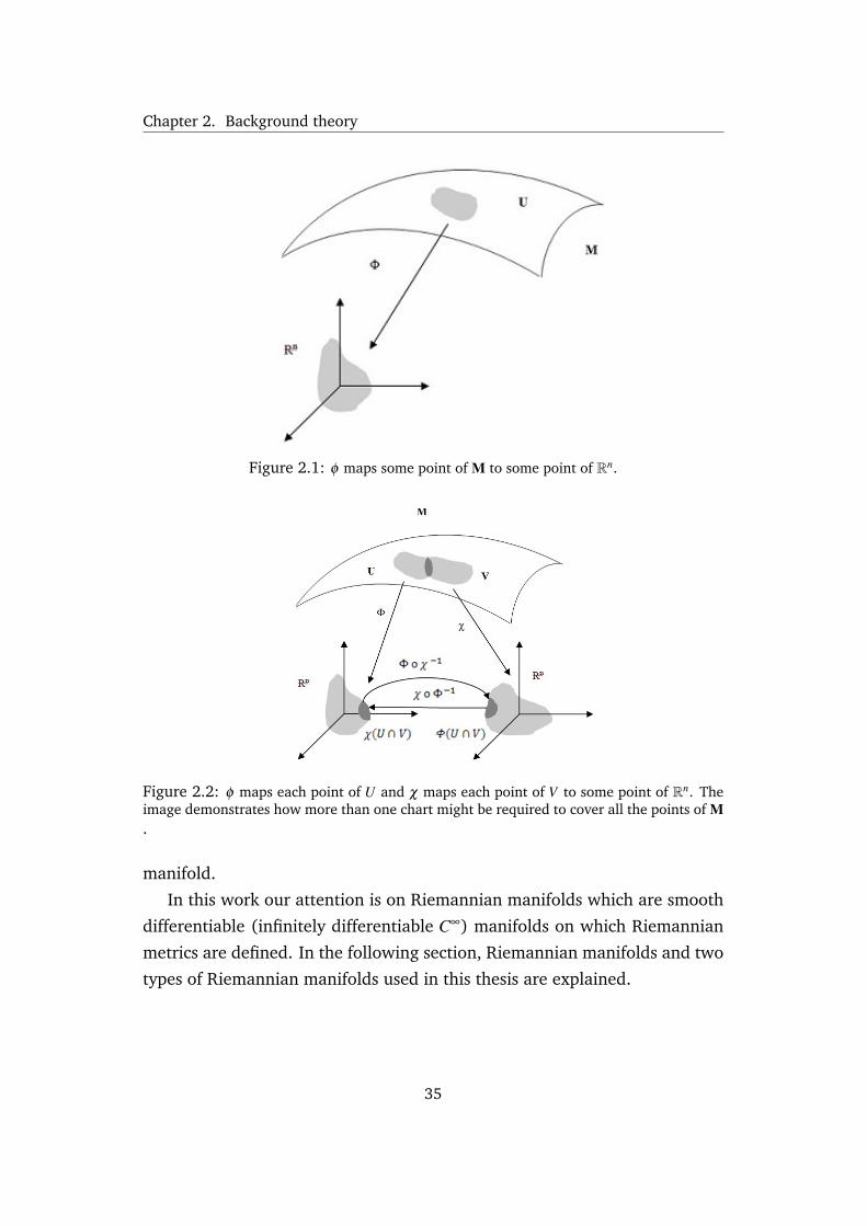
ordinates. Frequently, to cover all the points of M more than one chart is
required [DC11] (Fig. 2.2), which brings us to the definition of atlas Ck on
M. To understand the concept of atlas we need to first go through a number
of other definitions.
A function F :Rn→Rm is said to be differentiable of class Ck if there exist k
continuous partial derivatives for all of the real-valued functions f1, f2, · · · , fm,
where F(q) = ( f1(q), f2(q), · · · , fm(q)). Two charts (U,φ) and (V,χ) on M, are
then called Ck-related if U ∩V = ∅, or χ φ−1 and φ χ−1 are differentiable
of class Ck.
A collection of charts on M, (Ui,φ) form a Ck sub-atlas on M if for any pair
of i and j, (Ui,φi) and (U j,φ j) are Ck-related and M = U1∪U2∪ ·· · . Atlas Ck
on M is then formed from the collection of all the Ck-related charts with the
charts of a Ck sub-atlas on M.
Based on the above definitions we now define a Ck manifold of dimension
n to be a set M with a Ck atlas; then if k ≥ 1, then M is called a differentiable
34
Chapter 2. Background theory
Figure 2.1: φ maps some point of M to some point of Rn.
Figure 2.2: φ maps each point of U and χ maps each point of V to some point of Rn. Theimage demonstrates how more than one chart might be required to cover all the points of M.
manifold.
In this work our attention is on Riemannian manifolds which are smooth
differentiable (infinitely differentiable C∞) manifolds on which Riemannian
metrics are defined. In the following section, Riemannian manifolds and two
types of Riemannian manifolds used in this thesis are explained.
35
Chapter 2. Background theory
2.3 Riemannian Geometry
Riemannian manifolds are analytical manifolds endowed with a distance
measure which allows the measurement of similarity or dissimilarity (close-
ness or distance) of points. In other words, Reimannian manifolds are smooth
manifolds equipped with Riemannian metrics, which allow measurement of
geometric quantities such as distances and angles.
From this point on, when we say manifold, unless otherwise, we are refer-
ring to smooth differentiable manifolds. Before introducing more advanced
manifolds related concepts, we need to first go through some basic definitions
[Lee97], as follows:
Definition 2.3.1. A sub-manifold M of a smooth manifold M, is a smoothmanifold M together with an injective immersion ı : M→ M.
So, ı(M)⊂ M can be seen as an image of M. Although, we can consider M to
be a subset of M, in general the topology and structure of M may have only
little in common with that of M.
Definition 2.3.2. The inclusion map ı is considered to be an embedding, whenit is a homeomorphism onto its image with the subspace topology.
Definition 2.3.3. M is an embedded sub-manifold if the related inclusion mapı is an embedding.
Inference on Riemannian manifolds can be accomplished through embed-
ding the manifolds into higher dimensional Euclidean spaces. The most pop-
ular choice for embedding manifolds is achieved through tangent spaces [TPM08,
PTM06].
As tangent space plays an important role in analysing points over mani-
folds, in the following section we provide a more detailed introduction. Then
we introduce geodesic distance and look at the two types of Riemannian
manifolds used in this work, known as SPD manifolds and Grassmannian
manifolds. Finally, we explain the Stein divergence method used through
this thesis as a similarity measurement of points on SPD manifolds.
36
Chapter 2. Background theory
Figure 2.3: Relations between tangent spaces, tangent vectors, and geodesics. P1 and P2are points on the manifold, while TP1 and TP2 are tangent spaces at these points [TVC08].
2.3.1 Tangent Space
For each point P ∈M , a tangent space TP(M ) is the set of all tangent vectors
at the point P which can be defined as a vector space of derivations at the
point [Lui11]. Let P(t) be a matrix in Rn×m parametrised by a curve t such
that P(0) = In,p and P(t)T ×P(t) = I. Using the product rule, differentiating
P(t)T ×P(t) with respect to t produces [Lui11] :
P(t)T ddt
P(t)+ddt
P(t)T P(t) = 0 (2.2)
ddt
P(0)+ddt
P(0)T = 0 f or t = 0 (2.3)
The above equations indicate that the tangent space is the set of skew
symmetric matrices. Geometrically, one can refer to tangent space as a vec-
tor space with the origin shifted to x. Tangent spaces are critical aspects in
differential manifolds as they provide a bridge to a local vector space rep-
resentation of a manifold. To switch between manifold and tangent space
at point P, two operators, namely the exponential map exp(v) and logarithm
map log(P) are defined. Fig. 2.3 illustrates that for each point on the man-
ifold P ∈M , the tangent vector can be obtained through logarithmic map
log(P) = v where log(P) : M → TP(M ). For each vector starting from point X
37

Chapter 2. Background theory
in tangent space v ∈ Tp(M ) there exists an exponential map exp(v) = P where
exp(v) : TP(M )→M ‘pulls back’ the vector in the tangent space into a point
on the manifold [TVSC11].
38
Chapter 2. Background theory
2.3.2 Riemannian Metrics
In this section we briefly go through the definition of the Riemannian Met-
ric and geodesic distance which is then followed by detailing the relation
between geodesic distance and the curvature.
Definition 2.3.4. The Riemannian metric on a smooth manifold M is a sym-metric positive definite 2-tensor field g ∈ T 2 (M) [Lee97].
Thus a Riemannian metric determines an inner product on each tangent
space TpM.
Definition 2.3.5. The geodesic distance between two points X,Y ∈M , denotedby dg (X,Y), is defined as the minimum length over all possible smooth curvesbetween X and Y.
Thus a geodesic curve is a curve that locally minimises the distance between
points.
Curvature
It worth knowing that the possibility of computing geodesics on a Rieman-
nian manifold often is owed to the curved shape of the manifold [LTSC13].
The characterisation of the manifold curvature can be achieved through sev-
eral ways, here we briefly cover two of them:
1. sectional curvature
2. scalar curvature
If TX(M ) is a tangent space to a point X from a given Riemannian Mani-
fold M , sectional curvature is then specified with respect to a subspace of the
TX(M ) and can be obtained by using the Riemannian curvature tensor of the
M . The scalar curvature on the other hand, is the trace of the Ricci curvature
tensor and is twice the sum of sectional curvatures over all the subspaces of
TX(M ) [LTSC13].
To further clarify the above concepts, we consider the special case of 2
dimensional (2D) surfaces in R3. We first note that in the 2D space the
39
Chapter 2. Background theory
sectional and scalar curvature can be calculated through the Gaussian curva-
ture. In fact, in the 2D environment, the sectional curvature is equal to and
the scalar curvature is just twice the Gaussian curvature [LTSC13].
Let S : [0,1]2 → R3 be a parametrised surface with the mapping (u,v) 7→S(u,v) as the parametrisation of the S. We introduce two fundamental forms
of a surface which together defines certain geometric invariants of the sur-
face. The first fundamental form of S at (u,v) is given by the matrix below:
g(u,v) =
⟨
∂S∂u ,
∂S∂u
⟩ ⟨∂S∂u ,
∂S∂v
⟩⟨
∂S∂v ,
∂S∂u
⟩ ⟨∂S∂v ,
∂S∂v
⟩ (2.4)
where the vectors ∂S∂u ,
∂S∂v form a basis of the tangent space to S at (u,v). In
Eqn. (2.4) g(u,v) can be interpreted as a Riemannian metric on S.
The second fundamental form is defined below as representing the quadratic
approximation of the surface at point S:
Π =
⟨
∂S2
∂u2 , n⟩ ⟨
∂S2
∂u∂v , n⟩
⟨∂S2
∂u∂v , n⟩ ⟨
∂S2
∂v2 , n⟩ (2.5)
where n(u,v) = ∂S∂u×
∂S∂v is a vector normal to the surface at point (u,v) and
n = n(u,v)/ |n(u,v)| is the unit normal to the surface at that point.
Having defined the above concepts we can now build the definition of the
shape operator to be used as a descriptive tool for curvature properties. The
shape operator, which is a self-adjoint operator on the tangent space, is given
by the matrix below:
ς = g−1Π (2.6)
The Gaussian curvature can then be calculated through the shape operator
of the curved surface and is equivalent to the product of the eigenvalues of
the shape operator λ1λ2. Finally, the sectional curvature and scalar curvature
can be calculated accordingly [LTSC13].
40
Chapter 2. Background theory
2.3.3 Types of Riemannian Manifolds
Among various Riemannian manifolds, structures induced from subspaces
and Symmetric Positive Definite (SPD) matrices have been shown to be quite
useful in computer vision. Subspaces form a non-Euclidean and curved Rie-
mannian manifold known as a Grassmann manifold and SPD manifolds are
able to accommodate the effects of various image variations. For example,
a widely used approximation for photometric invariance, under conditions
of no shadowing and Lambertian reflectance, is a linear subspace [AMU97].
Moreover, subspaces can capture the dynamic properties of videos [TVSC11].
In this study we are interested in Grassmann manifolds (chapter 3) and the
manifolds of Symmetric-Positive-Definite matrices (SPD) (chapter 3, 4 and
5).
Symmetric positive definite matrices of size D×D, e.g. non-singular covari-
ance matrices, form a connected Riemannian manifold (Sym+D). The geodesic
distance between two points X and Y on Sym+D can be computed as
dG (X,Y) = trace
log2(
X−12 YX−
12
)(2.7)
In (2.7), log(·) is a matrix logarithm operator and can be computed through
Singular Value Decomposition (SVD). More specifically, let X = UΣUT be the
SVD of the symmetric matrix X, then
log(X) = U log(Σ)UT (2.8)
where log(Σ) is a diagonal matrices where the diagonal elements are equiva-
lent to the logarithms of the diagonal elements of matrix Σ.
To formally define a Grassmann manifold and its geometry, we need to
define the quotient space of the manifold. A quotient space of a manifold
can be described as the result of “gluing together” certain points of the man-
ifold. Formally, given ∼ψ as an equivalence relation on M , the quotient space
ϒ = M /∼ψ is defined to be the set of equivalence classes of elements of M ,
i.e., ϒ = [X] : X ∈M = [Y ∈M : Y∼ψ X] : X ∈M .
A Grassmann manifold is then defined as a quotient space of the special
orthogonal group1 SO(n) and is defined as a set of p-dimensional linear sub-1 Special orthogonal group SO(n) is the space of all n×n orthogonal matrices with the determinant
41
Chapter 2. Background theory
spaces of Rn.
In practice, an element X of G n, p is represented by an orthonormal basis
as a n× p matrix, i.e.,XT X = Ip. The geodesic distance between two points on
the Grassmann manifold can be computed as:
dG (X,Y) = ‖Θ‖2 (2.9)
where Θ = [θ1,θ2, · · · ,θp] is the principal angle vector, i.e.,:
cos(θi) = maxxi∈X, y j∈Y
xTi y j (2.10)
subject to xTi xi = yT
i yi = 1, xTi x j = yT
i y j = 0, i 6= j. The principal angles have the
property of θi ∈ [0,π/2] and can be computed through SVD of XT Y [EAS99].
+1. It is not a vector space but a differentiable manifold, i.e., it can be locally approximated by subsetsof a Euclidean space.
42
Chapter 2. Background theory
2.4 Symmetric Positive Definite Manifolds
Covariance matrices have recently been employed to describe images and
videos [Pen06, GIK10, TPM08], as they are known to provide compact and
informative feature description [CSBP11, AVN11]. Non-singular covariance
matrices are naturally symmetric positive definite matrices (SPD) which form
connected Riemannian manifolds when endowed with a Riemannian metric
over tangent spaces [Lan99]. Symmetric positive definite matrices (SPD)
arise in various problems in machine learning and computer vision. They
can be used to describe images and videos [GIK10, Pen06, TPM08], as they
naturally emerge in the form of covariance matrices and therefore provide
compact and informative feature descriptors [CSBP11]. In addition to cap-
turing feature correlations compactly, covariance matrices are known to be
robust to noise [AVN11]. A key aspect of covariance matrices is their natural
geometric property [Lan99], ie. they form a connected Riemannian mani-
fold. As such, the underlying distance and similarity functions might not be
accurately defined in Euclidean spaces [TPM08].
While the theory of learning in Euclidean spaces has been extensively de-
veloped, extensions to non-Euclidean spaces like Riemannian manifolds have
received relatively little attention. This is mainly due to difficulties of han-
dling the Riemannian structure as compared to straightforward Euclidean
geometry. For example, the manifold of SPD matrices is not closed under
normal matrix subtraction. As such, efficiently handling this structure is non-
trivial, due largely to two main challenges [SA11]: (i) defining divergence,
distance, or kernel functions on covariances is not easy; (ii) the numerical
burden is substantial, even for basic computations such as distances and clus-
tering.
To simplify the handling of Riemannian manifolds, inference is tradition-
ally achieved through first embedding the manifolds in higher dimensional
Euclidean spaces. A popular choice for embedding manifolds is through tan-
gent spaces [Lui11, PTM06, TPM08, VRCC05]. To be more specific, to ad-
dress the above issue, two lines of research have been proposed:
(1) embedding manifolds into tangent spaces [Lui11, PTM06, TPM08,
VRCC05];
43
Chapter 2. Background theory
(2) embedding into Reproducing Kernel Hilbert Spaces (RKHS), induced
by kernel functions [AHS13, HL09, HSWL12, STC04, SC11].
The former approach in effect maps manifold points to Euclidean spaces,
thereby enabling the use of existing Euclidean-based learning algorithms.
This comes at the cost of disregarding some of the manifold structure. For
instance, only distances between points to the tangent pole are equal to true
geodesic distances. This restriction might result in inaccurate modelling, as
the structure of the manifolds is only partially taken into account [HSWL12].
The latter approach addresses this by implicitly mapping points on the mani-
fold into RKHS, which can be considered to be a high dimensional Euclidean
space. Training data can be used to define a space that preserves manifold ge-
ometry [HSWL12]. While this approach allows the multitude of kernel-based
machine learning algorithms to be employed, existing Riemannian kernels
are either only applicable to subtypes of Riemannian manifolds (e.g., Grass-
mann manifolds) [HL09], or are pseudo-kernels [HSWL12], meaning they do
not satisfy all the conditions of true kernel functions [STC04]. The downside
is that existing Euclidean-based learning algorithms need to be kernelised,
which may not be trivial. Furthermore, the resulting methods can still have
high computational load, making them impractical to use in more complex
scenarios.
44
Chapter 2. Background theory
2.4.1 Stein Divergence
Consider X1 . . .Xn ∈ Symd+ to be a set of non-singular d×d-sized covariance
matrices, which are symmetric positive definite (SPD) matrices. These matri-
ces belong to a smooth differentiable topological spaces, known as SPD man-
ifolds. Before delving any further into this subject we first introduce one of
the most widely used Riemannian metric for SPD matrices which is known as
the Affine Invariant Riemannian Metrics (AIRM) [Pen06]. The AIRM induces
Riemannian structure which is invariant to inversion and similarity transfor-
mations. Despite its properties, learning methods using this approach have
to deal with computational challenges, such as employing computationally
expensive non-linear operators.
In this work, we endow the SPD manifold with the AIRM to induce the
Riemannian structure [Pen06]. As such, a point on manifold M can be
mapped to a tangent space using:
logXiXj = Xi
12 log(Xi
− 12 XjXi
− 12 )Xi
12 (2.11)
where Xi,Xj ∈ Symd+, Xi is the point where the tangent space is located
(i.e., tangent pole) and Xj is the point that we would like to map into the
tangent space TXiM ; log(·) is the matrix logarithm. The inverse function
that maps points on a particular tangent space into the manifold is:
expXiy = Xi
12 exp(Xi
− 12 yXi
− 12 )Xi
12 (2.12)
where Xi ∈ Symd+ is again the tangent pole; y∈TXiM is a point in the tangent
space TXiM ; exp(·) is the matrix exponential.
From the above functions, we now define the shortest distance between
two points on the manifold. The distance, here called geodesic distance, is
represented as the minimum length of the curvature path that connects two
points [Pen06]:
d2g (Xi,Xj) = trace
log2(Xi
− 12 XjXi
− 12 )
(2.13)
The above mapping functions can be computationally expensive. We can
also use the recently introduced Stein divergence [Sra12] to determine simi-
45

Chapter 2. Background theory
larities between points on the SPD manifold. Its symmetrised form is:
Jφ (X,Y), log(
det(
X+Y2
))− 1
2log(det(XY)) (2.14)
The Stein divergence kernel can then be defined as:
K(X,Y) = exp−σJφ (X,Y) (2.15)
under the condition of σ ∈ 12 ,
22 , ...,
d−12 to ensure that the kernel matrix
formed by Eqn. (2.15) is positive definite [HSHL12].
46
Chapter 3
Graph-Embedding DiscriminantAnalysis on Riemannian Manifoldsfor Visual Recognition
3.1 Overview
In this chapter1 we propose a solution for the problem of Discriminant Analy-
sis (DA) on Riemannian manifolds through RKHS space. The algorithm uses
a graph-based local Discriminant Analysis that utilises both within-class and
between class similarity graphs to characterise intra-class compactness and
inter-class separability respectively. We then validate the performance of the
proposed method on several classification tasks, including face and object
recognition, texture classification and person re-identification.
1 The method proposed in this chapter was published as a book chapter in ‘Graph Embedding forPattern Analysis’ [ASHL13]
47
Chapter 3. Graph-Embedding Discriminant Analysis on Riemannian Manifolds forVisual Recognition
3.2 Introduction
Inference on manifold spaces can be achieved by embedding the manifolds
in higher dimensional Euclidean spaces, which can be considered as flatten-
ing the manifolds. In the literature, the most popular choice for embedding
manifolds is through considering tangent spaces [TPM08, TVSC11]. Two
bold examples are the pedestrian detection system by Tuzel et al. [TPM08]
and non-linear mean shift [CM02] by Subbarao et al. [SM09]. Nevertheless,
flattening the manifold through tangent spaces is not without drawbacks. For
example, only distances between points to the tangent pole are equal to true
geodesic distances. This is restrictive and may lead to inaccurate modelling.
Instead of using tangent spaces to do inference on manifolds, we pro-
pose to embed Riemannian manifolds into Reproducing Kernel Hilbert Spaces
(RKHS). This in turn opens the door for employing many kernel-based ma-
chine learning algorithms [STC04]. As such, we tackle the problem of Dis-
criminant Analysis (DA) on Riemannian manifolds through RKHS space and
propose a graph-based local DA that utilises both within-class and between-
class similarity graphs to characterise intra-class compactness and inter-class
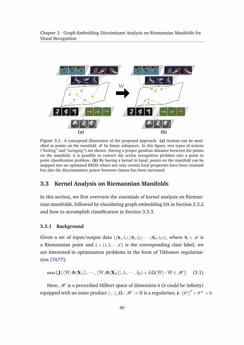
separability, respectively. See Fig. 3.1 for a conceptual example. Our graph-
based DA is inspired by findings in the Euclidean space that explain why the
conventional formalism of DA is not optimal when data comprises outliers
and multi-modal classes and contains outliers. Our experiments for several
recognition problems show that considerable gains in discrimination accu-
racy can be obtained by exploiting the geometrical structure and local infor-
mation on Riemannian manifolds.
48
Chapter 3. Graph-Embedding Discriminant Analysis on Riemannian Manifolds forVisual Recognition
(a) (b)
Figure 3.1: A conceptual illustration of the proposed approach. (a) Actions can be mod-elled as points on the manifold M by linear subspaces. In this figure, two types of actions(”kicking” and ”swinging”) are shown. Having a proper geodesic distance between the pointson the manifold, it is possible to convert the action recognition problem into a point topoint classification problem. (b) By having a kernel in hand, points on the manifold can bemapped into an optimised RKHS where not only certain local properties have been retainedbut also the discriminatory power between classes has been increased.
3.3 Kernel Analysis on Riemannian Manifolds
In this section, we first overview the essentials of kernel analysis on Rieman-
nian manifolds, followed by elucidating graph embedding DA in Section 3.3.2
and how to accomplish classification in Section 3.3.3.
3.3.1 Background
Given a set of input/output data (X1, l1),(X2, l2), · · · ,(XN , lN), where Xi ∈M is
a Riemannian point and li ∈ 1,2, · · · ,C is the corresponding class label, we
are interested in optimisation problems in the form of Tikhonov regularisa-
tion [TA77]:
maxJ(〈W,Φ(X1)〉, · · · ,〈W,Φ(XN)〉, l1, · · · , lN)+λΩ(W) : W ∈H (3.1)
Here, H is a prescribed Hilbert space of dimension h (h could be infinity)
equipped with an inner product 〈·, ·〉, Ω : H → R is a regulariser, J :(Rh)N×Y N → R
49
Chapter 3. Graph-Embedding Discriminant Analysis on Riemannian Manifolds forVisual Recognition
is a cost function. For certain choices of the regulariser, solving (3.1) reduces
to identifying N parameters and not the dimension of H . This is more for-
mally explained by the representer theorem [STC04] which states that the
solution W of (3.1) is a linear combination of the inputs when the regulariser
is the square of the Hilbert space norm. For vector Hilbert spaces, this result
is simple to prove and dates back to 1970s [KW70]. Argyriou et al. [AMP09]
showed that the representer theorem holds for matrix Hilbert spaces as well.
Implicitly embedding Riemannian manifolds into RKHS is achieved through
a Riemannian kernel. A function k : M ×M → R+ is a Riemannian kernel pro-
vided that it is positive definite and well defined for all X ∈M .
For the Grassmann manifold Xi ∈ GD,m, the latter criterion means that the
kernel should be invariant to various representations of the subspaces, i.e.,,k(X,Y) = k(XQ1,YQ2), ∀ Q1,Q2 ∈ O(m), where O(m) indicates orthonormal matri-
ces of order m [HL08]. The repertoire of Grassmann kernels includes Binet-
Cauchy [WS03] and projection kernels [HL08]. Furthermore, the first canon-
ical correlation of two subspaces forms a pseudo kernel2 on Grassmann man-
ifolds [HSSL11]. The three kernels are respectively shown below:
kBC(X,Y) = det(XT YYT X
)(3.2)
kproj(X,Y) = Tr(XT YYT X
)(3.3)
kCC(X,Y) = maxx∈X, y∈Y
xT y (3.4)
For the Sym+D, in [HSWL12] a pseudo kernel based on geodesic distances
was devised as followed:
kR (X,Y) = exp−σ−1dG (X,Y) (3.5)
where dG (X,Y) is obtained using (2.7). Very recently, Sra et al. introduced
the Stein kernel using Bregman matrix divergence as follows [Sra12]:
k(X,Y) = e−σS(X,Y) = 2dσ
√det(X)σ det(Y)σ
det(X+Y)σ(3.6)
2 A pseudo kernel is a function where the positive definiteness is not guaranteed to be satisfied forwhole range of the function’s parameters. Nevertheless, it is possible to convert a pseudo kernel into atrue kernel, as discussed for example in [CGG+09].
50
Chapter 3. Graph-Embedding Discriminant Analysis on Riemannian Manifolds forVisual Recognition
In (3.6), S(X,Y) is the symmetric Stein divergence and defined as:
S(X,Y), log(
det(
X+Y2
))− 1
2log(det(XY)) , for X,Y 0 (3.7)
3.3.2 Graph Embedding Discriminant Analysis on Riemannian Mani-folds
A graph (V,G) in our context refers to a collection of vertices or nodes, V,
and a collection of edges that connect pairs of vertices. We note that G is
a symmetric matrix with elements describing the similarity between pairs of
vertices. Moreover, the diagonal matrix D and the Laplacian matrix L of a
graph are defined as L = D−G, with the diagonal elements of D obtained as
D(i, i) = ∑ j G(i, j).
Given N labelled points X = (Xi, li)Ni=1 from the underlying Riemannian
manifold M , where Xi ∈ RD×m and li ∈ 1,2, · · · ,C, with C denoting the number
of classes, the local geometrical structure of M can be modelled by building
a within-class similarity graph Gw and a between-class similarity graph Gb.
The simplest forms of Gw and Gb are based on the nearest neighbour graphs
defined below:
Gw(i, j) =
1, if Xi ∈ Nw(X j) or X j ∈ Nw(Xi)
0, otherwise(3.8)
Gb(i, j) =
1, if Xi ∈ Nb(X j) or X j ∈ Nb(Xi)
0, otherwise(3.9)
In (3.8), Nw(Xi) is the set of νw neighbours
X1i ,X2
i , ...,Xvi, sharing the same
label as li. Similarly in (3.9), Nb(Xi) contains νb neighbours having different
labels. We note that more complex similarity graphs, like heat kernel graphs,
can also be used to encode distances between points on Riemannian mani-
folds [Ros97].
Our aim is to simultaneously maximise a measure of discriminatory power
and preserve the geometry of points. This can be formalised by finding
W : Φ(Xi)→ Yi such that the connected points of Gw are placed as close as
51
Chapter 3. Graph-Embedding Discriminant Analysis on Riemannian Manifolds forVisual Recognition
possible, while the connected points of Gb are moved as far as possible. As
such, a mapping must be sought by optimising the following two objective
functions:
f1 = min12 ∑i, j ‖Yi−Y j‖2Gw(i, j) (3.10)
f2 = max12 ∑i, j ‖Yi−Y j‖2Gb(i, j) (3.11)
Eqn. ((3.10)) punishes neighbours in the same class if they are mapped
far away, while Eqn.((3.11)) punishes points of different classes if they are
mapped close together.
According to the representer theorem [STC04], the solution W= [γ1|γ2| · · · |γr],
can be expressed as a linear combination of data points, i.e.,, γ i = ∑Nj=1 wi, jφ (X j).
More specifically:
Yi = (〈γ1,φ (Xi)〉 ,〈γ2,φ (Xi)〉 , · · · ,〈γr,φ (Xi)〉)T (3.12)
Since 〈γ l ,φ (Xi)〉= ∑Nj=1 wl, j Tr
(φ (X j)
Tφ (Xi)
)= ∑
Nj=1 wl, jk (X j,Xi), Yi = WT Ki, with Ki =
(k(Xi,X1),k(Xi,X2), · · · ,k(Xi,XN))T and
W =
w1,1 w1,2 · · · w1,r
w2,1 w2,2 · · · w2,r...
......
...
wN,1 wN,2 · · · wN,r
Plugging this back into (3.10) results in:
12 ∑i, j ‖Yi−Y j‖2Gw(i, j)
= 12 ∑i, j ‖WT Ki−WT K j‖2Gw(i, j)
= Tr(WTKDwKT W
)−Tr
(WTKGwKT W
) (3.13)
where K= [K1|K2| · · · |KN ]. Considering that Lb = Db−Wb, in a similar manner it
52
Chapter 3. Graph-Embedding Discriminant Analysis on Riemannian Manifolds forVisual Recognition
can be shown that (3.11) can be simplified to:
12 ∑i, j ‖Yi−Y j‖2Gb(i, j)
= Tr(WTKDbKT W
)−Tr
(WTKGbKT W
)= Tr
(WTKLbKT W
) (3.14)
To solve (3.10) and (3.11) simultaneously, we need to add the following
normalising constraint to the problem:
Tr(WTKDwKT W
)= 1 (3.15)
This constraint enables us to convert the minimisation problem (3.10)
into a maximisation one. Consequently, both equations can be combined
into one maximisation problem. Moreover, as we will see later, the imposed
constraint acts as a norm regulariser in the original Tikhonov problem (3.1),
thus satisfying the necessary condition of the representer theorem.
Plugging (3.15) into (3.10) results in:
min
Tr(WTKDwKT W
)−Tr
(WTKGwKT W
)= min
1−Tr
(WTKGwKT W
)= max
Tr(WTKGwKT W
) (3.16)
subject to the constraint shown in (3.15). As a result, the max versions of
(3.10) and (3.11) can be merged by the Lagrangian method as follows:
max
Tr(WTK(Lb +βGw)KT W
)subject to Tr
(WTKDwKT W
)= 1
(3.17)
where β is a Lagrangian multiplier. The solution to the optimisation in (3.17)
can be sought as the r largest eigenvectors of the following generalised eigen-
value problem [HSSL11]:
KLb +βGwKT W = λKDwKT W (3.18)
We note that in (3.18), the imposed constraint (3.15) serves as a norm reg-
ulariser and satisfies the representer theorem condition. Algorithm 1 assem-
53
Chapter 3. Graph-Embedding Discriminant Analysis on Riemannian Manifolds forVisual Recognition
bles all the above details into pseudo-code for Riemannian Graph Embedding
Discriminant Analysis (RGDA) training algorithm.
3.3.3 Classification
Upon acquiring the mapping W, the matching problem over Riemannian
manifolds is reduced to classification in vector spaces. More precisely, for any
query image set Xq, a vector representation using the kernel function and the
mapping W is acquired, i.e.,Vq =WT Kq, where Kq =(⟨
φ(X1),φ(Xq)⟩, · · · ,
⟨φ(XN),φ(Xq)
⟩)T .
Similarly, gallery points Xi are represented by r dimensional vectors Vi = WT Ki
and classification methods such as Nearest-Neighbour or Support Vector Ma-
chines [Bis06] can be employed to label Xq.
54
Chapter 3. Graph-Embedding Discriminant Analysis on Riemannian Manifolds forVisual Recognition
3.4 Experiments
In this section we investigate the performance of the proposed RGDA method
on several classification tasks, including face and object recognition, texture
classification and person re-identification. We evaluate RGDA over SPD man-
ifolds.
3.4.1 Experiments on SPD Manifolds
Mathematically, a covariance descriptor can be defined as follows: Let fiNi=1 ; fi ∈ Rn
be the feature vectors from the region of interest of an image or video, then
the Covariance Descriptor of this region C ∈ Sym+D is defined as:
C =1N
N
∑i=1
(fi−m)(fi−m)T (3.19)
where m is the mean feature vector, and N is the total number of training
data. In the following text, we study how covariance descriptors and the
induced geometry can be exploited for face recognition, texture classification
and people re-identification.
Face Recognition
For the face recognition task, we considered the subset ‘b’ of the FERET
dataset [PMRR00]. This subset includes 1400 images from 198 subjects.
Each image is closely cropped to merely include the face and then downsam-
pled to 64×64. Fig. 3.2 shows examples of the FERET dataset.
To evaluate the performance, we created three tests with various pose an-
gles. In all the tests, training data consisted of the images labelled as ‘bj’, ‘bk’
and ‘bf’ (ie. frontal image with illumination, expression and small pose varia-
tions). Images marked as ‘bd’, ‘be’ and ‘bg’ (ie. non-frontal images) were used
as three separate test sets. In our method, each face image is represented by
a 43× 43 covariance matrix as a point on the Riemannian manifold. To this
end, for every pixel I(x,y), we then computed Gu,v(x,y) as the response of a 2D
Gabor wavelet [Lee96], centered at x,y with orientation u and scale v. To be
specific, we considered the number of scales and orientations to be 5 and 8,
55
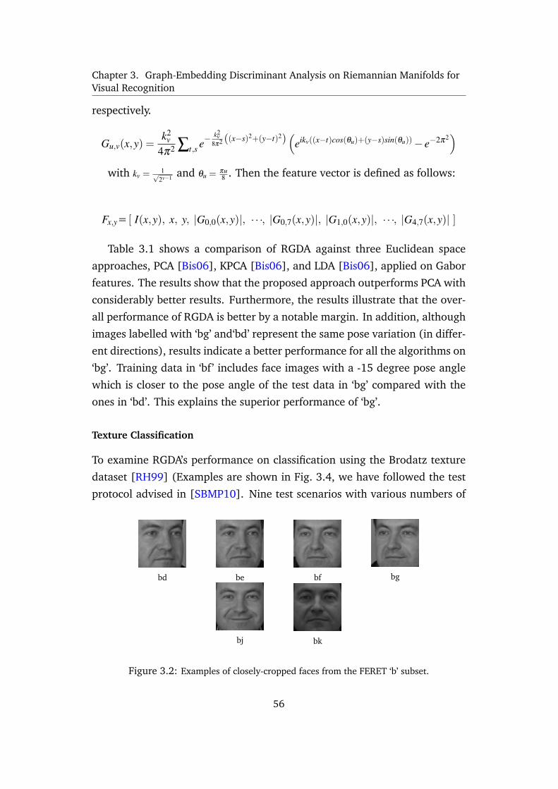
Chapter 3. Graph-Embedding Discriminant Analysis on Riemannian Manifolds forVisual Recognition
respectively.
Gu,v(x,y) =k2
v4π2 ∑t,s e−
k2v
8π2 ((x−s)2+(y−t)2)(
eikv((x−t)cos(θu)+(y−s)sin(θu))− e−2π2)
with kv =1√
2v−1 and θu =πu8 . Then the feature vector is defined as follows:
Fx,y= [ I(x,y), x, y, |G0,0(x,y)|, · · ·, |G0,7(x,y)|, |G1,0(x,y)|, · · ·, |G4,7(x,y)| ]
Table 3.1 shows a comparison of RGDA against three Euclidean space
approaches, PCA [Bis06], KPCA [Bis06], and LDA [Bis06], applied on Gabor
features. The results show that the proposed approach outperforms PCA with
considerably better results. Furthermore, the results illustrate that the over-
all performance of RGDA is better by a notable margin. In addition, although
images labelled with ‘bg’ and‘bd’ represent the same pose variation (in differ-
ent directions), results indicate a better performance for all the algorithms on
‘bg’. Training data in ‘bf’ includes face images with a -15 degree pose angle
which is closer to the pose angle of the test data in ‘bg’ compared with the
ones in ‘bd’. This explains the superior performance of ‘bg’.
Texture Classification
To examine RGDA’s performance on classification using the Brodatz texture
dataset [RH99] (Examples are shown in Fig. 3.4, we have followed the test
protocol advised in [SBMP10]. Nine test scenarios with various numbers of
bd be bf bg
bj bk
Figure 3.2: Examples of closely-cropped faces from the FERET ‘b’ subset.
56
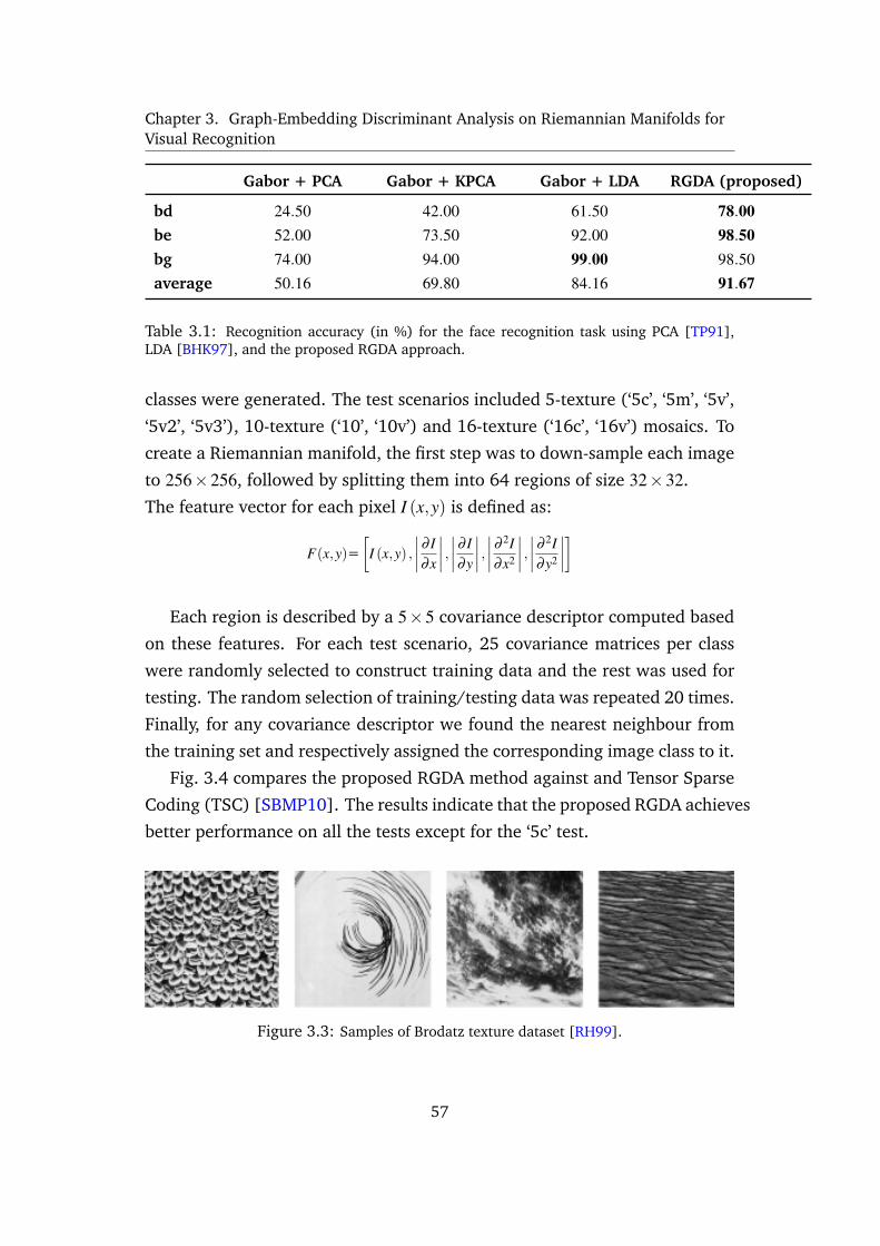
Chapter 3. Graph-Embedding Discriminant Analysis on Riemannian Manifolds forVisual Recognition
Gabor + PCA Gabor + KPCA Gabor + LDA RGDA (proposed)
bd 24.50 42.00 61.50 78.00be 52.00 73.50 92.00 98.50bg 74.00 94.00 99.00 98.50average 50.16 69.80 84.16 91.67
Table 3.1: Recognition accuracy (in %) for the face recognition task using PCA [TP91],LDA [BHK97], and the proposed RGDA approach.
classes were generated. The test scenarios included 5-texture (‘5c’, ‘5m’, ‘5v’,
‘5v2’, ‘5v3’), 10-texture (‘10’, ‘10v’) and 16-texture (‘16c’, ‘16v’) mosaics. To
create a Riemannian manifold, the first step was to down-sample each image
to 256×256, followed by splitting them into 64 regions of size 32×32.
The feature vector for each pixel I (x,y) is defined as:
F(x,y)=[
I (x,y) ,∣∣∣∣ ∂ I∂x
∣∣∣∣ , ∣∣∣∣ ∂ I∂y
∣∣∣∣ , ∣∣∣∣ ∂ 2I∂x2
∣∣∣∣ , ∣∣∣∣ ∂ 2I∂y2
∣∣∣∣]
Each region is described by a 5×5 covariance descriptor computed based
on these features. For each test scenario, 25 covariance matrices per class
were randomly selected to construct training data and the rest was used for
testing. The random selection of training/testing data was repeated 20 times.
Finally, for any covariance descriptor we found the nearest neighbour from
the training set and respectively assigned the corresponding image class to it.
Fig. 3.4 compares the proposed RGDA method against and Tensor Sparse
Coding (TSC) [SBMP10]. The results indicate that the proposed RGDA achieves
better performance on all the tests except for the ‘5c’ test.
Figure 3.3: Samples of Brodatz texture dataset [RH99].
57
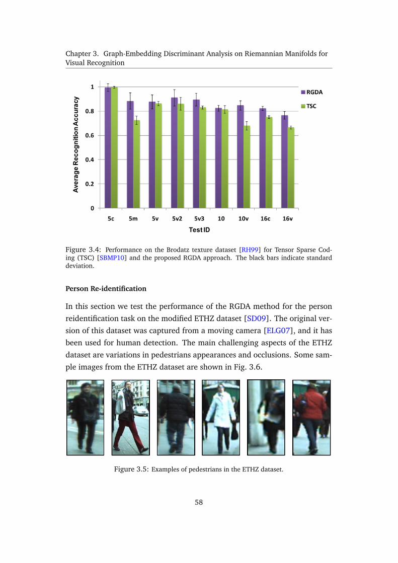
Chapter 3. Graph-Embedding Discriminant Analysis on Riemannian Manifolds forVisual Recognition
Figure 3.4: Performance on the Brodatz texture dataset [RH99] for Tensor Sparse Cod-ing (TSC) [SBMP10] and the proposed RGDA approach. The black bars indicate standarddeviation.
Person Re-identification
In this section we test the performance of the RGDA method for the person
reidentification task on the modified ETHZ dataset [SD09]. The original ver-
sion of this dataset was captured from a moving camera [ELG07], and it has
been used for human detection. The main challenging aspects of the ETHZ
dataset are variations in pedestrians appearances and occlusions. Some sam-
ple images from the ETHZ dataset are shown in Fig. 3.6.
Figure 3.5: Examples of pedestrians in the ETHZ dataset.
58
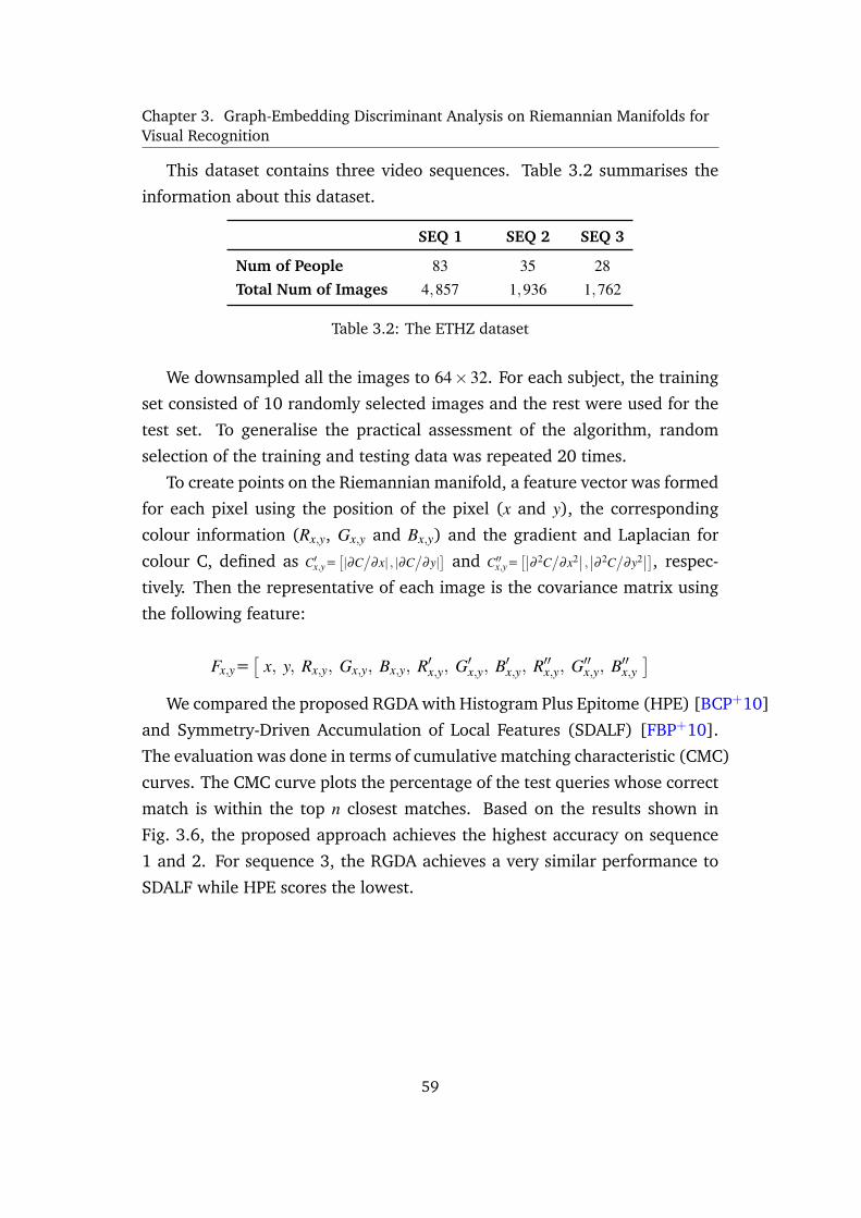
Chapter 3. Graph-Embedding Discriminant Analysis on Riemannian Manifolds forVisual Recognition
This dataset contains three video sequences. Table 3.2 summarises the
information about this dataset.
SEQ 1 SEQ 2 SEQ 3
Num of People 83 35 28Total Num of Images 4,857 1,936 1,762
Table 3.2: The ETHZ dataset
We downsampled all the images to 64×32. For each subject, the training
set consisted of 10 randomly selected images and the rest were used for the
test set. To generalise the practical assessment of the algorithm, random
selection of the training and testing data was repeated 20 times.
To create points on the Riemannian manifold, a feature vector was formed
for each pixel using the position of the pixel (x and y), the corresponding
colour information (Rx,y, Gx,y and Bx,y) and the gradient and Laplacian for
colour C, defined as C′x,y=[|∂C/
∂x| , |∂C/
∂y|]
and C′′x,y=[∣∣∂ 2C
/∂x2∣∣ , ∣∣∂ 2C
/∂y2∣∣], respec-
tively. Then the representative of each image is the covariance matrix using
the following feature:
Fx,y=[
x, y, Rx,y, Gx,y, Bx,y, R′x,y, G′x,y, B′x,y, R′′x,y, G′′x,y, B′′x,y]
We compared the proposed RGDA with Histogram Plus Epitome (HPE) [BCP+10]
and Symmetry-Driven Accumulation of Local Features (SDALF) [FBP+10].
The evaluation was done in terms of cumulative matching characteristic (CMC)
curves. The CMC curve plots the percentage of the test queries whose correct
match is within the top n closest matches. Based on the results shown in
Fig. 3.6, the proposed approach achieves the highest accuracy on sequence
1 and 2. For sequence 3, the RGDA achieves a very similar performance to
SDALF while HPE scores the lowest.
59
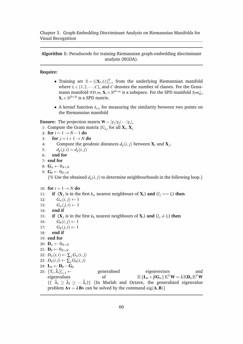
Chapter 3. Graph-Embedding Discriminant Analysis on Riemannian Manifolds forVisual Recognition
Algorithm 1: Pseudocode for training Riemannian graph-embedding discriminantanalysis (RGDA).
Require:
• Training set X= (Xi, li)Ni=1 from the underlying Riemannian manifold
where li ∈ 1,2, · · · ,C, and C denotes the number of classes. For the Grass-mann manifold G D,m, Xi ∈ RD×m is a subspace. For the SPD manifold Sym+
D,Xi ∈ RD×D is a SPD matrix.
• A kernel function ki j, for measuring the similarity between two points onthe Riemannian manifold
Ensure: The projection matrix W = [γ1|γ2| · · · |γr],1: Compute the Gram matrix [K]i j for all Xi, X j
2: for i = 1→ N−1 do3: for j = i+1→ N do4: Compute the geodesic distances dg(i, j) between Xi and X j.5: dg( j, i) = dg(i, j)6: end for7: end for8: Gw← 0N×N
9: Gb← 0N×N
% Use the obtained dg(i, j) to determine neighbourhoods in the following loop.
10: for i = 1→ N do11: if (X j is in the first kw nearest neighbours of Xi) and (l j == li) then12: Gw(i, j)← 113: Gw( j, i)← 114: end if15: if (X j is in the first kb nearest neighbours of Xi) and (l j 6= li) then16: Gb(i, j)← 117: Gb( j, i)← 118: end if19: end for20: Dw← 0N×N
21: Db← 0N×N
22: Dw(i, i)← ∑ j Gw(i, j)23: Db(i, i)← ∑ j Gb(i, j)24: Lb← Db−Gb25: ϒi, λir
i=1← generalised eigenvectors andeigenvalues of KLb +βGwKT W = λKDwKT W( λ1 ≥ λ2 ≥ ·· · λr) In Matlab and Octave, the generalised eigenvalueproblem Av = λBv can be solved by the command eig(A,B)
60
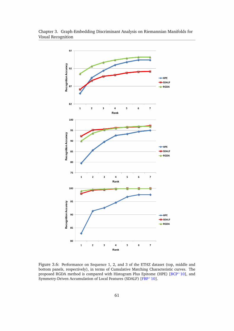
Chapter 3. Graph-Embedding Discriminant Analysis on Riemannian Manifolds forVisual Recognition
Figure 3.6: Performance on Sequence 1, 2, and 3 of the ETHZ dataset (top, middle andbottom panels, respectively), in terms of Cumulative Matching Characteristic curves. Theproposed RGDA method is compared with Histogram Plus Epitome (HPE) [BCP+10], andSymmetry-Driven Accumulation of Local Features (SDALF) [FBP+10].
61
Chapter 4
Relational Divergence BasedClassification on RiemannianManifolds
This chapter proposes a method for performing direct classification on mani-
fold. The method suggests presenting each SPD matrix through its similarity
vector to a number of other SPD matrices. The suggested method employs
the recently introduced Stein divergence to reduce the computational com-
plexity of the algorithm. Creating similarity vectors effectively converts the
classification problems on manifolds, which is a complex problem, into the
problem of finding appropriate machinery over the space of similarities.
In section 4.1 we detail the main method and validate it by testing the
algorithm using experiments on face recognition, texture classification and
person re-identification. The result illustrates that in comparison to well-
known methods, the proposed approach achieves a significant improvement
in image classification, while also being several orders of magnitude faster.
Then we specify a feature set in section 4.2 for addressing the person re-
identification task, and then test the method with a new feature set on the
two well known datasets for person re-identification. The results confirm that
in comparison to well-known person re-identification methods, the proposed
approach obtains a reasonable improvement in image classification, while
also being computationally competitive.
62

Chapter 4. Relational Divergence Based Classification on Riemannian Manifolds
4.1 Relational Divergence Based Classification
4.1.1 Overview
In this section1 we propose a method for performing direct classification on
manifold. More specifically, we propose a new method for analysing Rie-
mannian manifolds, where embedding into Euclidean spaces is not explicitly
required. To this end, we propose to represent Riemannian points through
their similarities to a set of reference points on the manifold, with the aid
of the recently proposed Stein divergence, which is a symmetrised version of
Bregman matrix divergence. Classification problems on manifolds are then
effectively converted into the problem of finding appropriate machinery over
the space of similarities, which can be tackled by conventional Euclidean
learning methods such as linear discriminant analysis. Experiments on face
recognition, person re-identification and texture classification show that the
proposed method outperforms state-of-the-art approaches, such as Tensor
Sparse Coding, Histogram Plus Epitome and Riemannian Locality Preserving
Projection.
1The method proposed in this chapter was published in IEEE Winter conference on Applications ofComputer Vision (WACV) 2014 [AHS13]
63
Chapter 4. Relational Divergence Based Classification on Riemannian Manifolds
4.1.2 Introduction
To avoid embedding into Euclidean spaces or RKHS, we explore the concept
of learning the classifier by relying only on the computed distance matrix
(similarity matrix) of the related training data. Given a set of training points
on a manifold, the idea is to employ the similarity between points as features.
More specifically, for each query point to be classified, a similarity to each
class is obtained, forming a similarity vector. We obtain each similarity with
the aid of the recently proposed Stein divergence [Sra12]. The classification
task on manifolds is hence converted into a task in the space of similarity
vectors, which can be tackled using learning methods devised for Euclidean
spaces. Experiments on several vision tasks (person re-identification, face
recognition and texture recognition), show that this new approach outper-
forms several state-of-the-art methods.
64
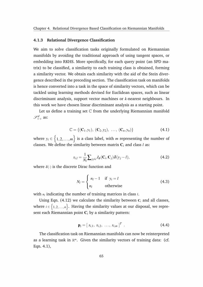
Chapter 4. Relational Divergence Based Classification on Riemannian Manifolds
4.1.3 Relational Divergence Classification
We aim to solve classification tasks originally formulated on Riemannian
manifolds by avoiding the traditional approach of using tangent spaces, or
embedding into RKHS. More specifically, for each query point (an SPD ma-
trix) to be classified, a similarity to each training class is obtained, forming
a similarity vector. We obtain each similarity with the aid of the Stein diver-
gence described in the preceding section. The classification task on manifolds
is hence converted into a task in the space of similarity vectors, which can be
tackled using learning methods devised for Euclidean spaces, such as linear
discriminant analysis, support vector machines or k-nearest neighbours. In
this work we have chosen linear discriminant analysis as a starting point.
Let us define a training set C from the underlying Riemannian manifold
S d++ as:
C= (C1,y1), (C2,y2), . . . , (Cn,yn) (4.1)
where yi ∈
1,2, . . . ,m
is a class label, with m representing the number of
classes. We define the similarity between matrix Ci and class l as:
si,l =1Nl
∑ j 6=i Jφ (Ci,C j)δ (y j− l), (4.2)
where δ (·) is the discrete Dirac function and
Nl =
nl−1 if yi = l
nl otherwise(4.3)
with nl indicating the number of training matrices in class l.
Using Eqn. (4.12) we calculate the similarity between Ci and all classes,
where i ∈
1,2, . . . ,n. Having the similarity values at our disposal, we repre-
sent each Riemannian point Ci by a similarity pattern:
pi = [ si,1, si,2, . . . , si,m ]T . (4.4)
The classification task on Riemannian manifolds can now be reinterpreted
as a learning task in Rm. Given the similarity vectors of training data: (cf.
Eqn. 4.1),
65
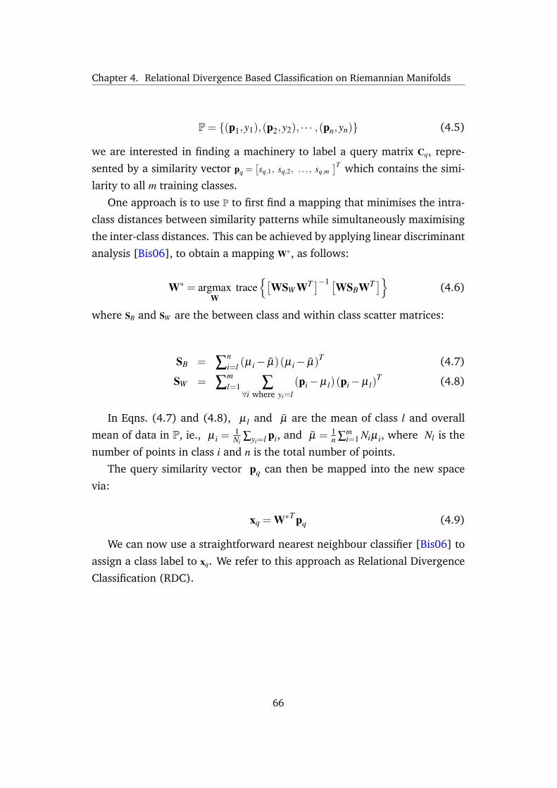
Chapter 4. Relational Divergence Based Classification on Riemannian Manifolds
P= (p1,y1),(p2,y2), · · · ,(pn,yn) (4.5)
we are interested in finding a machinery to label a query matrix Cq, repre-
sented by a similarity vector pq =[sq,1, sq,2, . . . , sq,m
]T which contains the simi-
larity to all m training classes.
One approach is to use P to first find a mapping that minimises the intra-
class distances between similarity patterns while simultaneously maximising
the inter-class distances. This can be achieved by applying linear discriminant
analysis [Bis06], to obtain a mapping W∗, as follows:
W∗ = argmaxW
trace[
WSW WT ]−1 [WSBWT ] (4.6)
where SB and SW are the between class and within class scatter matrices:
SB = ∑ni=l (µ i− µ)(µ i− µ)T (4.7)
SW = ∑ml=1 ∑∀i where yi=l
(pi−µ l)(pi−µ l)T (4.8)
In Eqns. (4.7) and (4.8), µ l and µ are the mean of class l and overall
mean of data in P, ie., µ i =1Ni
∑yi=l pi, and µ = 1n ∑
mi=1 Niµ i, where Nl is the
number of points in class i and n is the total number of points.
The query similarity vector pq can then be mapped into the new space
via:
xq = W∗T pq (4.9)
We can now use a straightforward nearest neighbour classifier [Bis06] to
assign a class label to xq. We refer to this approach as Relational Divergence
Classification (RDC).
66
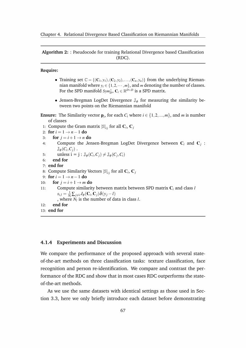
Chapter 4. Relational Divergence Based Classification on Riemannian Manifolds
Algorithm 2: : Pseudocode for training Relational Divergence based Classification(RDC).
Require:
• Training set C= (C1,y1),(C2,y2), . . . ,(Cn,yn) from the underlying Rieman-nian manifold where yi ∈ 1,2, · · · ,m, and m denoting the number of classes.For the SPD manifold Sym+
D, Ci ∈ RD×D is a SPD matrix.
• Jensen-Bregman LogDet Divergence Jφ for measuring the similarity be-tween two points on the Riemannian manifold
Ensure: The Similarity vector pi, for each Ci where i ∈ 1,2, ...,m, and m is numberof classes
1: Compute the Gram matrix [S]i j for all Ci, C j
2: for i = 1→ n−1 do3: for j = i+1→ n do4: Compute the Jensen-Bregman LogDet Divergence between Ci and C j :
Jφ (Ci,C j) .5: unless i = j : Jφ (Ci,C j) 6= Jφ (C j,Ci)6: end for7: end for8: Compute Similarity Vectors [S]i j for all Ci, C j
9: for i = 1→ n−1 do10: for j = i+1→ m do11: Compute similarity between matrix between SPD matrix Ci and class l
si,l =1Nl
∑ j 6=i Jφ (Ci,C j)δ (y j− l), where Nl is the number of data in class l.
12: end for13: end for
4.1.4 Experiments and Discussion
We compare the performance of the proposed approach with several state-
of-the-art methods on three classification tasks: texture classification, face
recognition and person re-identification. We compare and contrast the per-
formance of the RDC and show that in most cases RDC outperforms the state-
of-the-art methods.
As we use the same datasets with identical settings as those used in Sec-
tion 3.3, here we only briefly introduce each dataset before demonstrating
67

Chapter 4. Relational Divergence Based Classification on Riemannian Manifolds
Figure 4.1: Performance on the Brodatz texture dataset [RH99] for LogE-SR [GIK10,YHL+10], Tensor Sparse Coding (TSC) [SBMP10], Riemannian Locality Preserving Projec-tion (RLPP) [HSWL12] and the proposed RDC method.
our results. For more detail about the datasets and settings we refer the
reader to Section 3.3 of this thesis.
4.1.5 Texture Classification
We use the Brodatz texture dataset [RH99] and follow the test protocol pre-
sented in [SBMP10]. We use nine test scenarios with various number of
classes were generated.
Fig. 4.1 shows the performance of the proposed RDC method against
several state-of-the-art methods: log-Euclidean sparse representation (logE-
SR) [GIK10, YHL+10], Tensor Sparse Coding (TSC) [SBMP10] and Local-
ity Preserving Projection (RLPP) [HSWL12]. The results indicate that RDC
achieves better performance in 7 out of 9 tests.
68
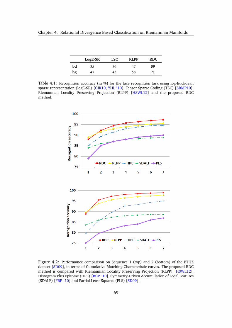
Chapter 4. Relational Divergence Based Classification on Riemannian Manifolds
LogE-SR TSC RLPP RDC
bd 35 36 47 59bg 47 45 58 71
Table 4.1: Recognition accuracy (in %) for the face recognition task using log-Euclideansparse representation (logE-SR) [GIK10, YHL+10], Tensor Sparse Coding (TSC) [SBMP10],Riemannian Locality Preserving Projection (RLPP) [HSWL12] and the proposed RDCmethod.
Figure 4.2: Performance comparison on Sequence 1 (top) and 2 (bottom) of the ETHZdataset [SD09], in terms of Cumulative Matching Characteristic curves. The proposed RDCmethod is compared with Riemannian Locality Preserving Projection (RLPP) [HSWL12],Histogram Plus Epitome (HPE) [BCP+10], Symmetry-Driven Accumulation of Local Features(SDALF) [FBP+10] and Partial Least Squares (PLS) [SD09].
69
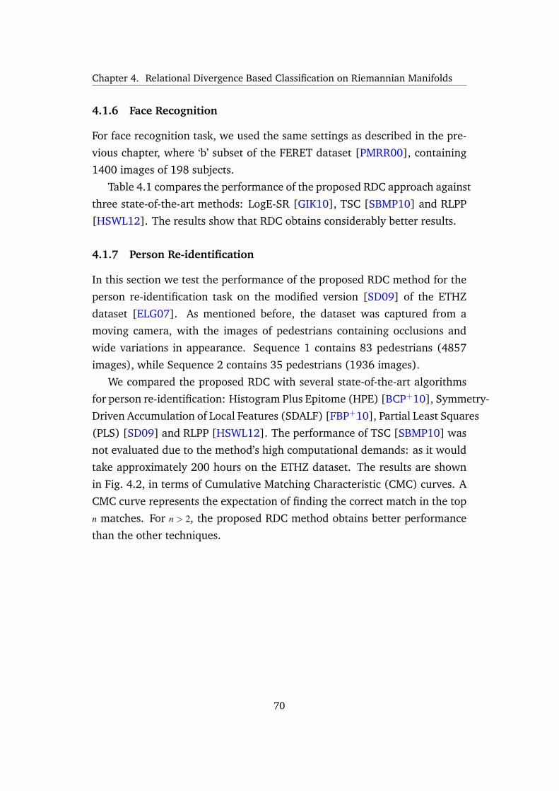
Chapter 4. Relational Divergence Based Classification on Riemannian Manifolds
4.1.6 Face Recognition
For face recognition task, we used the same settings as described in the pre-
vious chapter, where ‘b’ subset of the FERET dataset [PMRR00], containing
1400 images of 198 subjects.
Table 4.1 compares the performance of the proposed RDC approach against
three state-of-the-art methods: LogE-SR [GIK10], TSC [SBMP10] and RLPP
[HSWL12]. The results show that RDC obtains considerably better results.
4.1.7 Person Re-identification
In this section we test the performance of the proposed RDC method for the
person re-identification task on the modified version [SD09] of the ETHZ
dataset [ELG07]. As mentioned before, the dataset was captured from a
moving camera, with the images of pedestrians containing occlusions and
wide variations in appearance. Sequence 1 contains 83 pedestrians (4857
images), while Sequence 2 contains 35 pedestrians (1936 images).
We compared the proposed RDC with several state-of-the-art algorithms
for person re-identification: Histogram Plus Epitome (HPE) [BCP+10], Symmetry-
Driven Accumulation of Local Features (SDALF) [FBP+10], Partial Least Squares
(PLS) [SD09] and RLPP [HSWL12]. The performance of TSC [SBMP10] was
not evaluated due to the method’s high computational demands: as it would
take approximately 200 hours on the ETHZ dataset. The results are shown
in Fig. 4.2, in terms of Cumulative Matching Characteristic (CMC) curves. A
CMC curve represents the expectation of finding the correct match in the top
n matches. For n > 2, the proposed RDC method obtains better performance
than the other techniques.
70
Chapter 4. Relational Divergence Based Classification on Riemannian Manifolds
4.2 RDC for Person Re-identification
4.2.1 Overview
In this chapter2 we extend our work in Section 4.1 to specifically address
the person re-identification task. Person re-identification is particularly chal-
lenging due to significant appearance changes across separate camera views.
In order to reidentify people, a representative human signature should ef-
fectively handle differences in illumination, pose and camera parameters.
While general appearance-based methods are modelled in Euclidean spaces,
it has been argued that some applications in image and video analysis are
better modelled via non-Euclidean manifold geometry. To this end, recent
approaches represent images as covariance matrices, and interpret such ma-
trices as points on Riemannian manifolds. As direct classification on such
manifolds can be difficult, in this chapter we propose to represent each man-
ifold point as a vector of similarities to class representers, via a recently
introduced form of Bregman matrix divergence known as the Stein diver-
gence. This is followed by using a discriminative mapping of similarity vec-
tors for final classification. The use of similarity vectors is in contrast to
the traditional approach of embedding manifolds into tangent spaces, which
can suffer from representing the manifold structure inaccurately. Compara-
tive evaluations on benchmark ETHZ and iLIDS datasets for the person re-
identification task show that the proposed approach achieves better perfor-
mance than recent techniques such as Histogram Plus Epitome, Partial Least
Squares, and Symmetry-Driven Accumulation of Local Features.
2The method proposed in this chapter was published in International Conference on Image Pro-cessing (ICIP) 2013 [AYHS13]
71
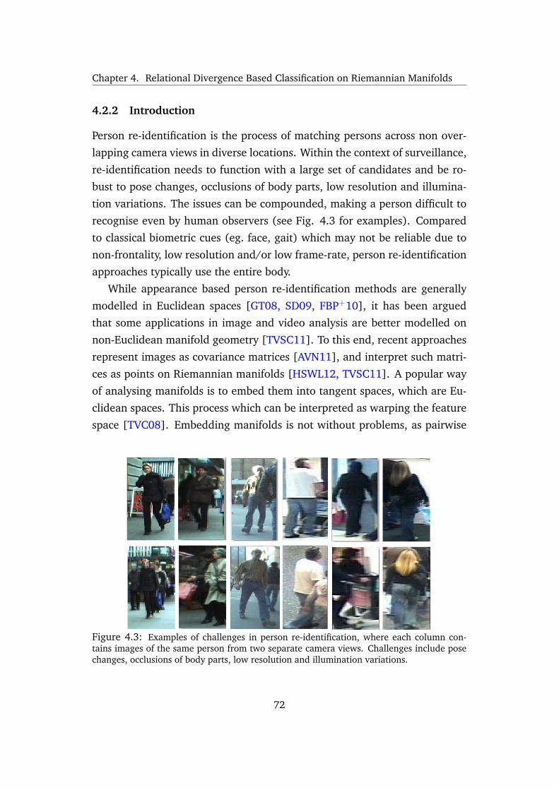
Chapter 4. Relational Divergence Based Classification on Riemannian Manifolds
4.2.2 Introduction
Person re-identification is the process of matching persons across non over-
lapping camera views in diverse locations. Within the context of surveillance,
re-identification needs to function with a large set of candidates and be ro-
bust to pose changes, occlusions of body parts, low resolution and illumina-
tion variations. The issues can be compounded, making a person difficult to
recognise even by human observers (see Fig. 4.3 for examples). Compared
to classical biometric cues (eg. face, gait) which may not be reliable due to
non-frontality, low resolution and/or low frame-rate, person re-identification
approaches typically use the entire body.
While appearance based person re-identification methods are generally
modelled in Euclidean spaces [GT08, SD09, FBP+10], it has been argued
that some applications in image and video analysis are better modelled on
non-Euclidean manifold geometry [TVSC11]. To this end, recent approaches
represent images as covariance matrices [AVN11], and interpret such matri-
ces as points on Riemannian manifolds [HSWL12, TVSC11]. A popular way
of analysing manifolds is to embed them into tangent spaces, which are Eu-
clidean spaces. This process which can be interpreted as warping the feature
space [TVC08]. Embedding manifolds is not without problems, as pairwise
Figure 4.3: Examples of challenges in person re-identification, where each column con-tains images of the same person from two separate camera views. Challenges include posechanges, occlusions of body parts, low resolution and illumination variations.
72
Chapter 4. Relational Divergence Based Classification on Riemannian Manifolds
distances between arbitrary points on a tangent space may not represent the
structure of the manifold accurately [HSWL12, HSHL12].
In this chapter we present a multi-shot appearance based person re-identification
method on Riemannian manifolds, where embedding the manifolds into tan-
gent spaces is not required. We adapt a recently proposed technique for
analysing Riemannian manifolds, where points on the manifolds are repre-
sented through their similarity vectors [AHS13]. The similarity vectors con-
tain similarities to class representers. We obtain each similarity with the aid
of a recently introduced form of Bregman matrix divergence known as the
Stein divergence [HSHL12, Sra12]. The classification task on manifolds is
hence converted into a task in the space of similarity vectors, which can be
tackled using learning methods devised for Euclidean spaces, such as Lin-
ear Discriminant Analysis [Bis06]. Unlike previous person re-identification
methods, the proposed method does not require separate settings for new
datasets.
73
Chapter 4. Relational Divergence Based Classification on Riemannian Manifolds
4.2.3 Previous Work
Given an image of an individual to be re-identified, the task of person re-
identification can be categorised into two main classes. (i) Single-vs-Single
(SvS), where there is only one image of each person in the gallery and one
in the probe; this can be seen as a one-to-one comparison. (ii) Multiple-vs-
Single (MvS), or multi-shot, where there are multiple images of each person
available in gallery and one image in the probe. Below we summarise several
person re-identification methods: Partial Least Squares (PLS) [SD09], Con-
text based method [ZGX09], Histogram Plus Epitome (HPE) [BCP+10], and
Symmetry-Driven Accumulation of Local Features (SDALF) [FBP+10].
The PLS method [SD09] first decomposes a given image into overlapping
blocks, and extracts a rich set of features from each block. Three types of fea-
tures are considered: textures, edges, and colours. The dimensionality of the
feature space is then reduced by employing Partial Least Squares regression
(PLSR) [WKJ85], which models relations between sets of observed variables
by means of latent variables. To learn a PLSR discriminatory model for each
person, one-against-all scheme is used [GK86]. Nearest neighbour is then
employed for classification.
The Context-based method [ZGX09] enriches the description of a person
by contextual visual knowledge from surrounding people. The method rep-
resents a group by considering two descriptors: (a) ‘center rectangular ring
ratio-occurrence’ descriptor, which describes the information ratio of visual
words between and within various rectangular ring regions, and (b) ‘block
based ratio-occurrence’ descriptor, which describes local spatial information
between visual words that could be stable. For group image representation
only features extracted from foreground pixels are used to construct visual
words.
HPE [BCP+10] considers multiple instances of each person to create a
person signature. The structural element (STEL) generative model approach
[JPC+09] is employed for foreground detection. The combination of a global
(person level) HSV histogram and epitome regions of foreground pixels is
then calculated, where an image epitome [JFK03] is computed by collapsing
74

Chapter 4. Relational Divergence Based Classification on Riemannian Manifolds
the given image into a small collage of overlapped patches. The patches con-
tain the essence of textural, shape and appearance properties of the image.
Both the generic epitome (epitome mean) and local epitome (probability that
a patch is in an epitome) are computed.
SDALF [FBP+10] considers multiple instances of each person. Foreground
features are used to model three complementary aspects of human appear-
ance extracted from various body parts. First, for each pedestrian image,
axes of asymmetry and symmetry are found. Then, complementary aspects
of the person appearance are detected on each part, and their features are
extracted. To select salient parts of a given pedestrian image, the features are
then weighted by exploiting perceptual principles of symmetry and asymme-
try.
The above methods assume that classical Euclidean geometry is capable of
providing meaningful solutions (distances and statistics) for modelling and
analysing images and videos, which might not be always correct [TVC08].
Furthermore, they require separate parameter tuning for each dataset.
75
Chapter 4. Relational Divergence Based Classification on Riemannian Manifolds
4.2.4 Proposed approach
Our goal is to automatically re-identify a given person among a large set of
candidates in diverse locations over various non-overlapping camera views.
The proposed method is comprised of three main stages: (i) feature extrac-
tion and generation of covariance descriptors, (ii) measurement of similari-
ties on Riemannian manifolds via the Stein divergence, and (iii) creation of
similarity vectors and discriminative mapping for final classification. Each of
the stages is elucidated in more detail in the following subsections.
Feature Extraction and Covariance Descriptors
As per [BCP+10, FBP+10], to reduce the effect of varying background, fore-
ground pixels are extracted from each given image of a person via the STEL
generative model approach [JPC+09]. We note that it is also possible to use
more advanced approaches, such as [RSL13].
Based on preliminary experiments, for each each foreground pixel located
at (x,y), the following feature vector is calculated:
f = [ x, y, HSVxy, CIELABxy, Λxy, Θxy ]T (4.10)
where HSVxy = [Hxy,Sxy,Vxy] are the colour values of the HSV channels, employ-
ing histogram equalisation for channel V , CIELABxy = [Lxy,axy,bxy] are the values
of CIELAB colour space [AR05], while Λxy = [λ Rxy,λ
Gxy,λ
Bxy] and Θxy = [θ R
xy,θGxy,θ
Bxy] in-
dicate gradient magnitudes and orientations for each channel in RGB colour
space. We note that we have selected this relatively straightforward set of
features as a starting point, and that it is certainly possible to use other fea-
tures. However, a thorough evaluation of possible features is beyond the
scope of this work.
Given a set F = fiNi=1 of extracted features, with its mean represented by
µ, each image is represented as a covariance matrix:
C =1
N−1 ∑Ni=1(fi−µ)(fi−µ)T (4.11)
Representing an image with a covariance matrix has several advantages
[AVN11]: (i) it is a low-dimensional (compact) representation that is inde-
pendent of image size, (ii) the impact of noisy samples is reduced via the
averaging during covariance computation, and (iii) it is a straightforward
76

Chapter 4. Relational Divergence Based Classification on Riemannian Manifolds
method of fusing correlated features.
77
Chapter 4. Relational Divergence Based Classification on Riemannian Manifolds
4.2.5 Similarity Vectors and Discriminative Mapping
For each query point (an SPD matrix) to be classified, a similarity to each
training class is obtained, forming a similarity vector. We obtain each simi-
larity with the aid of the Stein divergence described in the preceding section.
The classification task on manifolds is hence converted into a task in the space
of similarity vectors, which can be tackled using learning methods devised for
Euclidean spaces.
Given a training set of points on a Riemannian manifold, X= (X1,y1), . . . , (Xn,yn),
where yi ∈
1,2, . . . ,m
is a class label, and m is the number of classes, we define
the similarity between matrix Xi and class l as:
si,l =1Nl
∑ j 6=i Jφ (Xi,X j)δ (y j− l) (4.12)
where δ (·) is the discrete Dirac function and
Nl =
nl−1 if yi = l
nl otherwise(4.13)
where nl is the number of training matrices in class l. Using Eqn. (4.12), the
similarity between Xi and all classes is obtained, where i ∈
1,2, . . . ,n. Each
matrix Xi is hence represented by a similarity vector:
si = [ si,1, si,2, . . . , si,m ]T (4.14)
Classification on Riemannian manifolds can now be reinterpreted as a
learning task in Rm. Given the similarity vectors of training data, S= (s1,y1), · · · ,(sn,yn),
we seek a way to label a query matrix Xq, represented by a similarity vector
sq =[sq,1, sq,2, . . . , sq,m
]T . As a starting point, we have chosen linear discrimi-
nant analysis [Bis06], where we find a mapping W∗ that minimises the intra-
class distances while simultaneously maximising inter-class distances:
78

Chapter 4. Relational Divergence Based Classification on Riemannian Manifolds
W∗ = argmaxW
trace[
WSW WT ]−1 [WSBWT ] (4.15)
where SB and SW are the between class and within class scatter matrices[Bis06].
The query similarity vector sq can then be mapped into the new space via:
xq = W∗T sq (4.16)
We can now use a straightforward nearest neighbour classifier [Bis06]
to assign a class label to xq. We shall refer to this approach as Relational
Divergence Classification (RDC).
79
Chapter 4. Relational Divergence Based Classification on Riemannian Manifolds
4.2.6 Experiments and Discussion
In this section we evaluate the proposed RDC approach by providing com-
parisons against several methods on two person re-identification datasets:
iLIDS [ZGX09] and ETHZ [ELG07, SD09]. The VIPeR dataset [GBT07b] was
not used as it only has one image from each person in the gallery, and is hence
not suitable for testing MvS approaches. Each dataset covers various aspects
and challenges of the person re-identification task. The results are shown in
terms of the Cumulative Matching Characteristic (CMC) curves, where each
CMC curve represents the expectation of finding the correct match in the top
n matches.
In order to show the improvement caused by using similarity vectors in
conjunction with linear discriminant analysis, we also evaluate the perfor-
mance of directly using the Stein divergence in conjunction with a nearest
neighbour classifier (ie. direct classification on manifolds, without creating
similarity vectors). We refer to this approach as the direct Stein method.
4.2.7 iLIDS Dataset
The iLIDS dataset is a publicly available video dataset capturing real sce-
narios at an airport arrival hall under a multi-camera CCTV network. From
these videos a dataset of 479 images of 119 pedestrians was extracted and
the images were normalised to 128× 64 pixels (height × width) [ZGX09].
The extracted images were chosen from non-overlapping cameras, and are
subject to illumination changes and occlusions [ZGX09].
We randomly selected N images for each person to build the gallery set,
while the remaining images form the probe set. The whole procedure is
repeated 10 times in order to estimate an average CMC curve. We com-
pared the performance of the proposed RDC approach against the direct
Stein method, as well as the algorithms described in Section 4.2.3 (SDALF
and Context based) for a commonly used setting of N = 3. The results, shown
in Fig. 4.4, indicate that the proposed method generally outperforms the
other techniques. The results also show that the use of similarity vectors in
conjunction with linear discriminant analysis is preferable to directly using
the Stein divergence.
80
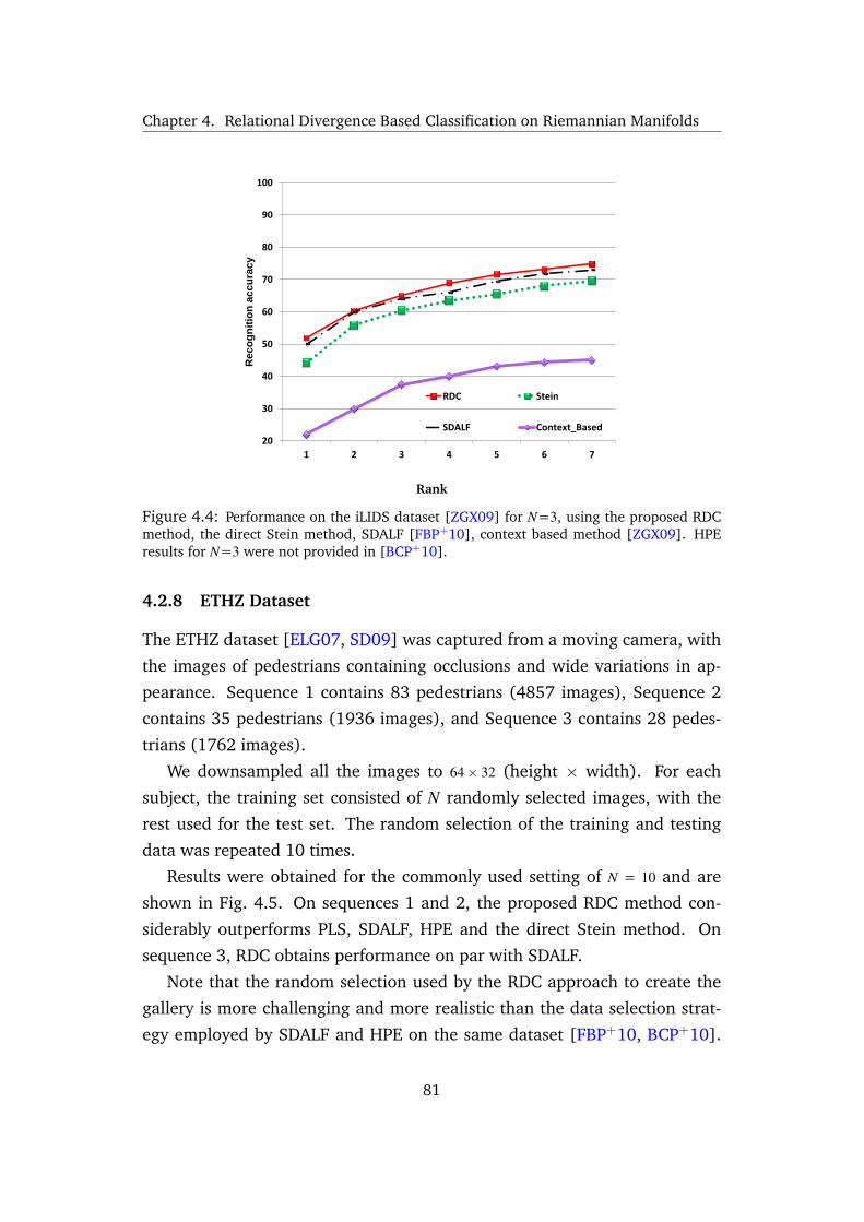
Chapter 4. Relational Divergence Based Classification on Riemannian Manifolds
20
30
40
50
60
70
80
90
100
1 2 3 4 5 6 7
Reco
gn
itio
n a
ccu
racy
RDC Stein
SDALF Context_Based
Rank
Figure 4.4: Performance on the iLIDS dataset [ZGX09] for N=3, using the proposed RDCmethod, the direct Stein method, SDALF [FBP+10], context based method [ZGX09]. HPEresults for N=3 were not provided in [BCP+10].
4.2.8 ETHZ Dataset
The ETHZ dataset [ELG07, SD09] was captured from a moving camera, with
the images of pedestrians containing occlusions and wide variations in ap-
pearance. Sequence 1 contains 83 pedestrians (4857 images), Sequence 2
contains 35 pedestrians (1936 images), and Sequence 3 contains 28 pedes-
trians (1762 images).
We downsampled all the images to 64× 32 (height × width). For each
subject, the training set consisted of N randomly selected images, with the
rest used for the test set. The random selection of the training and testing
data was repeated 10 times.
Results were obtained for the commonly used setting of N = 10 and are
shown in Fig. 4.5. On sequences 1 and 2, the proposed RDC method con-
siderably outperforms PLS, SDALF, HPE and the direct Stein method. On
sequence 3, RDC obtains performance on par with SDALF.
Note that the random selection used by the RDC approach to create the
gallery is more challenging and more realistic than the data selection strat-
egy employed by SDALF and HPE on the same dataset [FBP+10, BCP+10].
81

Chapter 4. Relational Divergence Based Classification on Riemannian Manifolds
SDALF and HPE both apply clustering beforehand on the original frames,
and then select randomly one frame for each cluster to build their gallery set.
In this way they can ensure that their gallery set includes the keyframes to
use for the multi-shot signature calculation. In contrast, we haven’t applied
any clustering for the proposed RDC method in order to be closer to real life
scenarios.
82
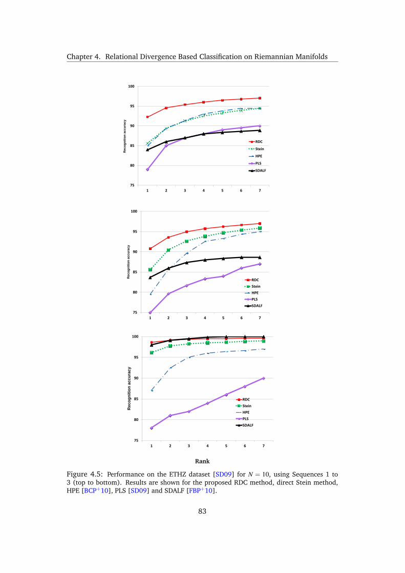
Chapter 4. Relational Divergence Based Classification on Riemannian Manifolds
75
80
85
90
95
100
1 2 3 4 5 6 7
Re
co
gn
itio
n a
cc
ura
cy
RDC
Stein
HPE
PLS
SDALF
75
80
85
90
95
100
1 2 3 4 5 6 7
Reco
gn
itio
n a
ccu
racy
RDC
Stein
HPE
PLS
SDALF
75
80
85
90
95
100
1 2 3 4 5 6 7
Reco
gn
itio
n a
ccu
racy
RDC
Stein
HPE
PLS
SDALF
Rank
Figure 4.5: Performance on the ETHZ dataset [SD09] for N = 10, using Sequences 1 to3 (top to bottom). Results are shown for the proposed RDC method, direct Stein method,HPE [BCP+10], PLS [SD09] and SDALF [FBP+10].
83
Chapter 5
Random Projections on Manifoldsof Symmetric Positive DefiniteMatrices for Image Classification
5.1 Overview
This chapter1 proposes the use of random projection over SPD manifold for
the purpose of scenes analysis. We offer a novel solution that allows SPD ma-
trices to be used with unmodified Euclidean-based learning algorithms, with
the true manifold shape well-preserved. Specifically, we propose to project
SPD matrices using a set of random projection hyperplanes over RKHS into
a random projection space, which leads to representing each matrix as a
vector of projection coefficients. Experiments on face recognition, person re-
identification and texture classification show that the proposed approach out-
performs several recent methods, such as Tensor Sparse Coding, Histogram
Plus Epitome, Riemannian Locality Preserving Projection and Relational Di-
vergence Classification.
1The algorithm proposed in this work is accepted in IEEE Winter conference on Applications ofComputer Vision (WACV) 2014.
84
Chapter 5. Random Projections on Manifolds of Symmetric Positive DefiniteMatrices for Image Classification
5.2 Introduction
We propose a method that employs a mapping technique to create a space
which preserves the manifold geometry while can be considered of as Eu-
clidean.
Specifically, we first embed SPD manifold points into RKHS via the Stein
Divergence Kernel [Sra12]. We then generate random projection hyper-
planes in RKHS and project the embedded points via the method proposed
in [KG09]. Finally, as the underlying space can be thought as Euclidean,
any appropriate Euclidean-based learning machinery can be applied. In this
chapter, we study the efficacy of this embedding method for classification
tasks. We show that the space is only as effective as the completeness of
the training data generating the random projection hyperplanes, and address
this through the use of synthetic data to augment training data. Experiments
on several vision tasks (person re-identification, face recognition and texture
recognition), show that the proposed approach outperforms several state-of-
the-art methods.
85
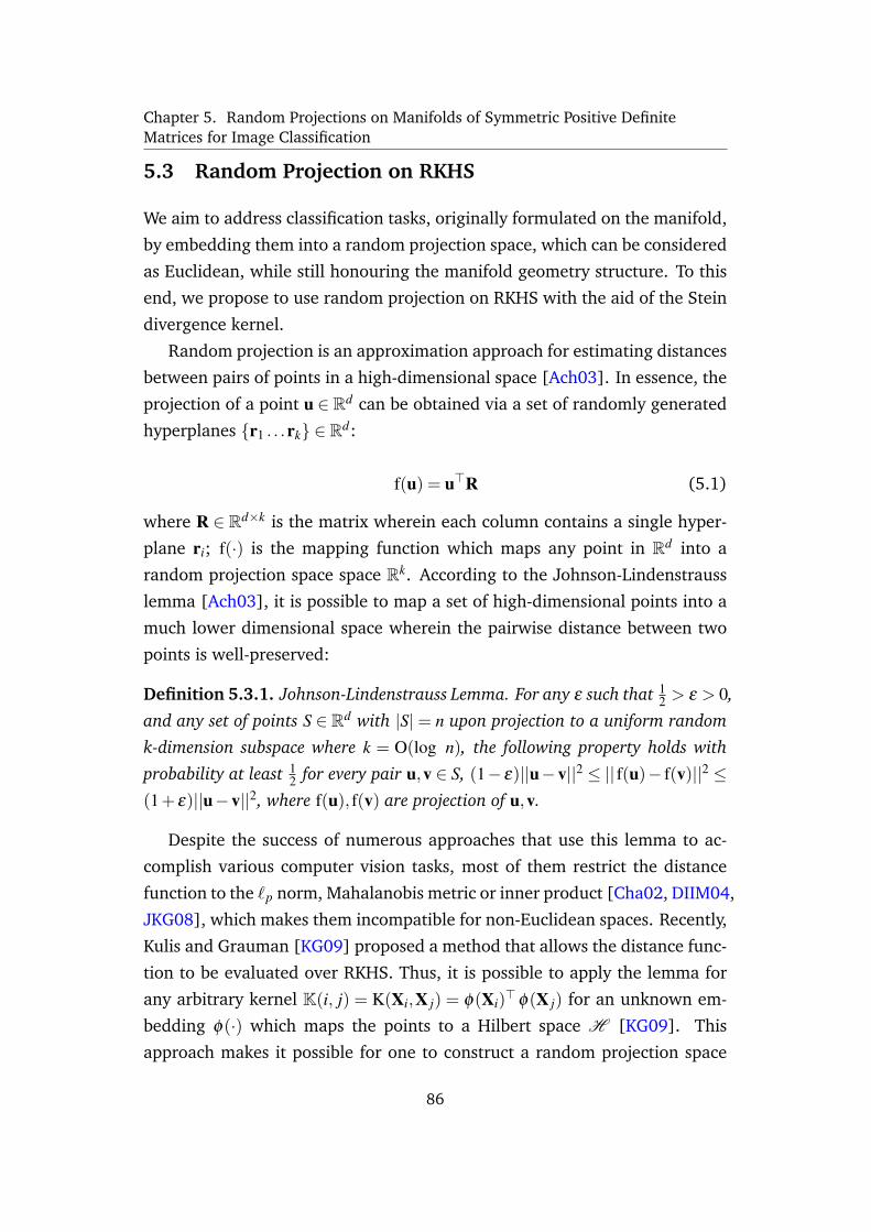
Chapter 5. Random Projections on Manifolds of Symmetric Positive DefiniteMatrices for Image Classification
5.3 Random Projection on RKHS
We aim to address classification tasks, originally formulated on the manifold,
by embedding them into a random projection space, which can be considered
as Euclidean, while still honouring the manifold geometry structure. To this
end, we propose to use random projection on RKHS with the aid of the Stein
divergence kernel.
Random projection is an approximation approach for estimating distances
between pairs of points in a high-dimensional space [Ach03]. In essence, the
projection of a point u ∈ Rd can be obtained via a set of randomly generated
hyperplanes r1 . . .rk ∈ Rd:
f(u) = u>R (5.1)
where R ∈ Rd×k is the matrix wherein each column contains a single hyper-
plane ri; f(·) is the mapping function which maps any point in Rd into a
random projection space space Rk. According to the Johnson-Lindenstrauss
lemma [Ach03], it is possible to map a set of high-dimensional points into a
much lower dimensional space wherein the pairwise distance between two
points is well-preserved:
Definition 5.3.1. Johnson-Lindenstrauss Lemma. For any ε such that 12 > ε > 0,
and any set of points S ∈ Rd with |S|= n upon projection to a uniform randomk-dimension subspace where k = O(log n), the following property holds withprobability at least 1
2 for every pair u,v ∈ S, (1− ε)||u−v||2 ≤ || f(u)− f(v)||2 ≤(1+ ε)||u−v||2, where f(u), f(v) are projection of u,v.
Despite the success of numerous approaches that use this lemma to ac-
complish various computer vision tasks, most of them restrict the distance
function to the `p norm, Mahalanobis metric or inner product [Cha02, DIIM04,
JKG08], which makes them incompatible for non-Euclidean spaces. Recently,
Kulis and Grauman [KG09] proposed a method that allows the distance func-
tion to be evaluated over RKHS. Thus, it is possible to apply the lemma for
any arbitrary kernel K(i, j) = K(Xi,X j) = φ(Xi)>φ(X j) for an unknown em-
bedding φ(·) which maps the points to a Hilbert space H [KG09]. This
approach makes it possible for one to construct a random projection space
86
Chapter 5. Random Projections on Manifolds of Symmetric Positive DefiniteMatrices for Image Classification
on an SPD manifold, where the manifold structure is well-preserved.
The main idea of our proposed approach, denoted as Random Projection
On SPD manifold for ImagE Classification (ROSE), is to first map all points
on the manifold into RKHS, with an implicit mapping function φ(·), via the
Stein divergence kernel. This is followed by mapping all the points in the
RKHS φ(Xi) ∈H into a random projection space Rk. To achieve this we
follow the Kulis-Grauman approach [KG09] by randomly generating a set
of hyperplanes over the RKHS r1 . . .rk ∈H which is restricted to be ap-
proximately Gaussian. As the embedding function φ(·) is unknown, then the
generation process is done indirectly via a weighted sum of the subset of the
given training sets.
To this end, consider each data point φ(Xi) from the training set as a
vector from some underlying distribution D with unknown mean µ and un-
known covariance σ . Let S be a set of t training exemplars chosen i.i.d. from
D, then zt =1t ∑i∈S φ(Xi) is defined over S. According to the central limit the-
orem for sufficiently large t, the random vector zt =√
t(zt −µ) is distributed
according to the multi-variate Gaussian N (µ,σ) [Ric07]. Then if a whiten-
ing transformation is applied, it results in ri = σ−12 zt which follows N (0,I)
distribution in Hilbert space H . Therefore, the i-th coefficient of each vector
in the random projection space is defined as:
φ(Xi)T
σ− 1
2 zt (5.2)
The mean µ and covariance σ need to be approximated from training
data. A set of p objects is chosen to form the first p items of a reference set:
φ(X1), . . . ,φ(Xp). Then the mean is implicitly estimated as µ = 1p ∑
pi=1 φ(Xi),
and the covariance matrix σ is also formed over the p samples. Eqn. (5.2)
can be solved using a similar approach as for Kernel PCA, which requires pro-
jecting onto the eigenvectors of the covariance matrix [KG09]. Let the eigen-
decomposition of σ be UVUT , then σ−12 =UV
12UT , and therefore Eqn. (5.2)
can be rewritten as below [KG09]:
φ(Xi)TUV
12UT zt (5.3)
Then let K be defined as a kernel matrix over the p randomly selected
87
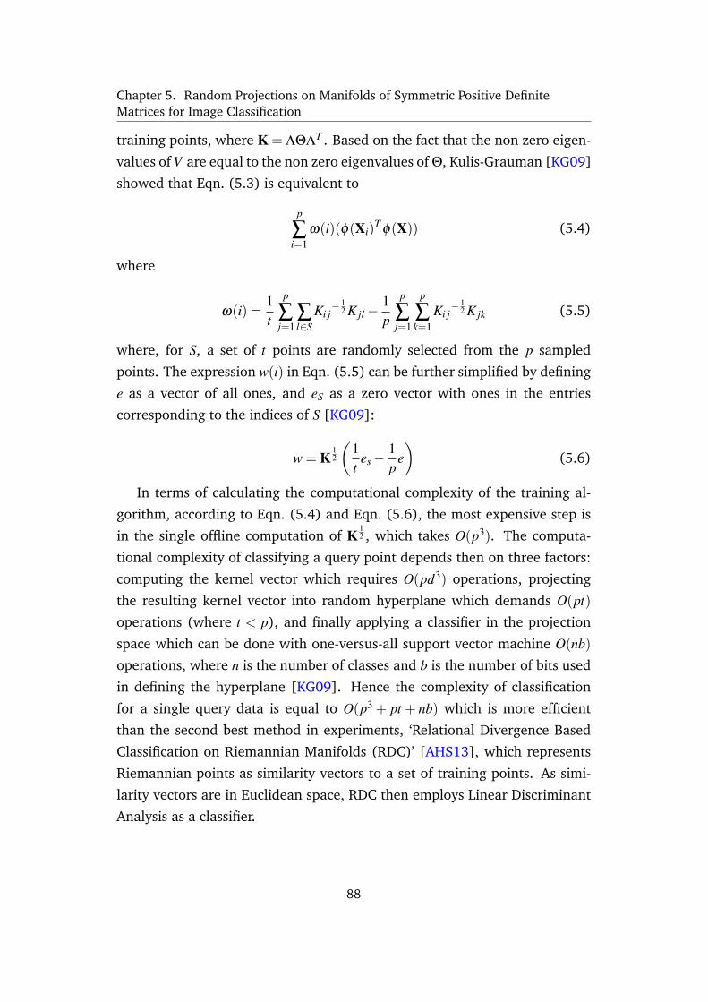
Chapter 5. Random Projections on Manifolds of Symmetric Positive DefiniteMatrices for Image Classification
training points, where K = ΛΘΛT . Based on the fact that the non zero eigen-
values of V are equal to the non zero eigenvalues of Θ, Kulis-Grauman [KG09]
showed that Eqn. (5.3) is equivalent to
p
∑i=1
ω(i)(φ(Xi)T
φ(X)) (5.4)
where
ω(i) =1t
p
∑j=1
∑l∈S
Ki j− 1
2 K jl−1p
p
∑j=1
p
∑k=1
Ki j− 1
2 K jk (5.5)
where, for S, a set of t points are randomly selected from the p sampled
points. The expression w(i) in Eqn. (5.5) can be further simplified by defining
e as a vector of all ones, and eS as a zero vector with ones in the entries
corresponding to the indices of S [KG09]:
w = K12
(1t
es−1p
e)
(5.6)
In terms of calculating the computational complexity of the training al-
gorithm, according to Eqn. (5.4) and Eqn. (5.6), the most expensive step is
in the single offline computation of K12 , which takes O(p3). The computa-
tional complexity of classifying a query point depends then on three factors:
computing the kernel vector which requires O(pd3) operations, projecting
the resulting kernel vector into random hyperplane which demands O(pt)
operations (where t < p), and finally applying a classifier in the projection
space which can be done with one-versus-all support vector machine O(nb)
operations, where n is the number of classes and b is the number of bits used
in defining the hyperplane [KG09]. Hence the complexity of classification
for a single query data is equal to O(p3 + pt + nb) which is more efficient
than the second best method in experiments, ‘Relational Divergence Based
Classification on Riemannian Manifolds (RDC)’ [AHS13], which represents
Riemannian points as similarity vectors to a set of training points. As simi-
larity vectors are in Euclidean space, RDC then employs Linear Discriminant
Analysis as a classifier.
88
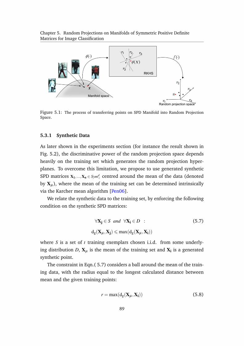
Chapter 5. Random Projections on Manifolds of Symmetric Positive DefiniteMatrices for Image Classification
Figure 5.1: The process of transferring points on SPD Manifold into Random ProjectionSpace.
5.3.1 Synthetic Data
As later shown in the experiments section (for instance the result shown in
Fig. 5.2), the discriminative power of the random projection space depends
heavily on the training set which generates the random projection hyper-
planes. To overcome this limitation, we propose to use generated synthetic
SPD matrices X1, ...,Xn ∈ Symd+ centred around the mean of the data (denoted
by Xµ), where the mean of the training set can be determined intrinsically
via the Karcher mean algorithm [Pen06].
We relate the synthetic data to the training set, by enforcing the following
condition on the synthetic SPD matrices:
∀Xj ∈ S and ∀Xi ∈ D : (5.7)
dg(Xµ ,Xj)6 max(dg(Xµ ,Xi))
where S is a set of t training exemplars chosen i.i.d. from some underly-
ing distribution D, Xµ is the mean of the training set and Xi is a generated
synthetic point.
The constraint in Eqn.( 5.7) considers a ball around the mean of the train-
ing data, with the radius equal to the longest calculated distance between
mean and the given training points:
r = max(dg(Xµ ,Xi)) (5.8)
89
Chapter 5. Random Projections on Manifolds of Symmetric Positive DefiniteMatrices for Image Classification
Then we need to generate SPD matrices which are located within r radius
from the mean (Eqn. 5.8). It is not trivial to generate SPD matrices which
follow the Eqn.(5.7), as it establishes a relation between the generated SPD
matrices and the original training points. To address this, we apply the re-
lationship between the geodesic distance and the given Riemannian metric
in a tangent space. Let Xi,Xj ∈ Symd+ be two points on the manifold and
xi,xj ∈ TXiM be the representing points on the tangent space TXiM . The
norm of vector xixj is equivalent to dg(Xi,Xj) [Pen06]. Therefore, it is possi-
ble to find a point Yi along the geodesic Xi and Xj whose geodesic distance
to Xi satisfies Eqn.(5.7).
Along with the above definitions, we introduce the following definition
and proposition:
Definition 5.3.2. Any point on an SPD manifold Xi ∈ Symd+ is said to have
normalised geodesic distance with respect to Xj ∈ Symd+ if and only if dg(Xi,Xj)=
1.
Proposition 5.3.3. For any two SPD matrices X,Xµ ∈ Symd+, there exists X on
the geodesic curve defined on X and Xµ , which has normalised geodesic distancewith respect to Xµ . The point X can be determined via: Xµ
12
(Xµ− 1
2 XXµ− 1
2
)cXµ
12 ,
where c = ζ
dg(X,Xµ ), for ζ = 1.
To prove the above proposition, we let X,Xµ ∈ Symd+ to be two given points
on an SPD manifold. In order to normalise the geodesic distance of X with
respect to Xµ , we map point X into tangent space TXµM . As a tangent space
is considered as Euclidean space where the distance between X and tangent
pole Xµ is preserved, Euclidean vector normalisation can be applied. Finally
the normalised point is mapped back to the manifold. These steps can be
presented as:
X = expXµ
(ζ
dg(Xµ ,X)logXµ
(X)
)(5.9)
By plugging in (2.11) and (2.12) we obtain:
X = Xµ
12 exp
(ζ
dg(Xµ ,X)log(Xµ
− 12 XXµ
− 12 )
)Xµ
12
90
Chapter 5. Random Projections on Manifolds of Symmetric Positive DefiniteMatrices for Image Classification
If we let c = ζ
dg(Xµ ,X) , based on the fact that X and Xµ are SPD matrices, we
arrive at:2
X = Xµ
12 exp
(log((Xµ
− 12 XXµ
− 12 )c))
Xµ
12
which proves that:
X = Xµ
12
(Xµ− 1
2 XXµ− 1
2
)cXµ
12 (5.10)
Having ζ is equal to 1 results in a normalised geodesic distance with re-
spect to Xµ . However in our case to satisfy Eqn. (5.7), we use ζ = δ ×max(dg(Xµ ,X j)), where δ ∈ [0,1] is a randomly generated number according
to uniform distribution.
2For the proof of logXc = c logX where X ∈ Symd+, refer to the appendix
91
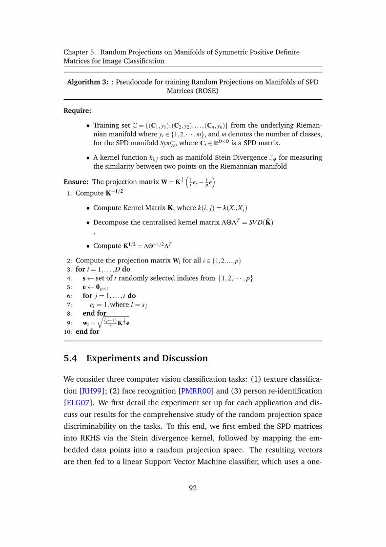
Chapter 5. Random Projections on Manifolds of Symmetric Positive DefiniteMatrices for Image Classification
Algorithm 3: : Pseudocode for training Random Projections on Manifolds of SPDMatrices (ROSE)
Require:
• Training set C= (C1,y1),(C2,y2), . . . ,(Cn,yn) from the underlying Rieman-nian manifold where yi ∈ 1,2, · · · ,m, and m denotes the number of classes,for the SPD manifold Sym+
D, where Ci ∈ RD×D is a SPD matrix.
• A kernel function ki, j such as manifold Stein Divergence Jφ for measuringthe similarity between two points on the Riemannian manifold
Ensure: The projection matrix W = K12
(1t es− 1
p e)
1: Compute K−1/2
• Compute Kernel Matrix K, where k(i, j) = k(Xi,X j)
• Decompose the centralised kernel matrix ΛΘΛT = SV D(K),
• Compute K1/2 = ΛΘ−1/2ΛT
2: Compute the projection matrix Wi for all i ∈ 1,2, ..., p3: for i = 1, . . . ,D do4: s← set of t randomly selected indices from 1,2, · · · , p5: e← 0p×16: for j = 1, . . . , t do7: el = 1,where l = s j
8: end for9: wi =
√(p−1)
t K12 e
10: end for
5.4 Experiments and Discussion
We consider three computer vision classification tasks: (1) texture classifica-
tion [RH99]; (2) face recognition [PMRR00] and (3) person re-identification
[ELG07]. We first detail the experiment set up for each application and dis-
cuss our results for the comprehensive study of the random projection space
discriminability on the tasks. To this end, we first embed the SPD matrices
into RKHS via the Stein divergence kernel, followed by mapping the em-
bedded data points into a random projection space. The resulting vectors
are then fed to a linear Support Vector Machine classifier, which uses a one-
92
Chapter 5. Random Projections on Manifolds of Symmetric Positive DefiniteMatrices for Image Classification
versus-all configuration for multi-class classification [FCH+08, STC04].
The parameter settings are as follows. As suggested in [KG09], we have
used t = min(30, 14n), where n is the number of samples chosen to create each
hyperplane. For the number of the random hyperplanes we have used vali-
dation data to choose one of n, 2n or 3n. Based on empirical observations on
validation sets, the number of synthetic samples was chosen as either n or m,
where m is the number of samples per class. In a similar manner, the value
of σ in Eqn. (2.15) was chosen from 1,2, . . . ,20.As we use the same datasets with identical setting as those used in Section
3.3, here we only briefly introduce each dataset before demonstrating our
results. For more details about the datasets and settings refer to Section 3.3
of this thesis.
We compare our proposed method, here denoted as Random Projection
On SPD manifold for ImagE Classification (ROSE), with several other em-
bedding approaches (tangent spaces, RKHS and hashing) as well as several
state-of-the-art methods. We also evaluate the effect of augmenting the train-
ing data with synthetic data points, and refer to this approach as ROSE with
Synthetic data (ROSES).
5.4.1 Person Re-Identification
For the person re-identification task we used the modified version [SD09] of
the ETHZ dataset [ELG07]. The dataset was captured from a moving camera,
with the images of pedestrians containing occlusions and wide variations in
appearance. Each image was represented as a covariance matrix of feature
vectors obtained at each pixel location.
For the task of texture classification, we use the Brodatz dataset [RH99].
We follow the test protocol presented in [SBMP10]. Accordingly, nine test
scenarios with various number of classes were generated, To create SPD ma-
trices, we follow [AHS13] by downsampling each image and then splitting it
into 64 regions. Each region is described by a covariance matrix formed from
the feature vectors introduced in section 3.3.
For face recognition task, the ‘b’ subset of the FERET dataset [PMRR00]
is used. Each image is first closely cropped to include only the face and then
downsampled. The tests with various pose angles were created to evaluate
93
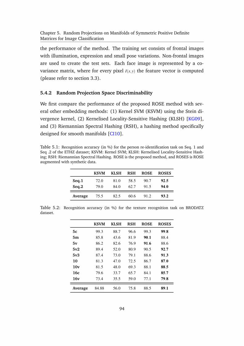
Chapter 5. Random Projections on Manifolds of Symmetric Positive DefiniteMatrices for Image Classification
the performance of the method. The training set consists of frontal images
with illumination, expression and small pose variations. Non-frontal images
are used to create the test sets. Each face image is represented by a co-
variance matrix, where for every pixel I(x,y) the feature vector is computed
(please refer to section 3.3).
5.4.2 Random Projection Space Discriminability
We first compare the performance of the proposed ROSE method with sev-
eral other embedding methods: (1) Kernel SVM (KSVM) using the Stein di-
vergence kernel, (2) Kernelised Locality-Sensitive Hashing (KLSH) [KG09],
and (3) Riemannian Spectral Hashing (RSH), a hashing method specifically
designed for smooth manifolds [CI10].
Table 5.1: Recognition accuracy (in %) for the person re-identification task on Seq. 1 andSeq .2 of the ETHZ dataset; KSVM: Kernel SVM; KLSH: Kernelised Locality-Sensitive Hash-ing; RSH: Riemannian Spectral Hashing. ROSE is the proposed method, and ROSES is ROSEaugmented with synthetic data.
KSVM KLSH RSH ROSE ROSES
Seq.1 72.0 81.0 58.5 90.7 92.5Seq.2 79.0 84.0 62.7 91.5 94.0
Average 75.5 82.5 60.6 91.2 93.2
Table 5.2: Recognition accuracy (in %) for the texture recognition task on BRODATZdataset.
KSVM KLSH RSH ROSE ROSES
5c 99.3 88.7 96.6 99.3 99.85m 85.8 43.6 81.9 90.1 88.45v 86.2 82.6 76.9 91.6 88.65v2 89.4 52.0 80.9 90.5 92.75v3 87.4 73.0 79.1 88.6 91.310 81.3 47.0 72.5 86.7 87.010v 81.5 48.0 69.3 88.1 88.516c 79.6 33.7 65.7 84.1 85.716v 73.4 35.5 59.0 77.1 79.8
Average 84.88 56.0 75.8 88.5 89.1
94
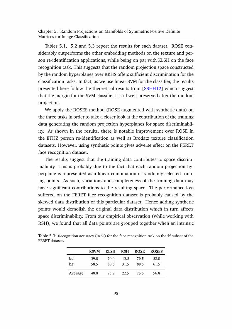
Chapter 5. Random Projections on Manifolds of Symmetric Positive DefiniteMatrices for Image Classification
Tables 5.1, 5.2 and 5.3 report the results for each dataset. ROSE con-
siderably outperforms the other embedding methods on the texture and per-
son re-identification applications, while being on par with KLSH on the face
recognition task. This suggests that the random projection space constructed
by the random hyperplanes over RKHS offers sufficient discrimination for the
classification tasks. In fact, as we use linear SVM for the classifier, the results
presented here follow the theoretical results from [SSHH12] which suggest
that the margin for the SVM classifier is still well-preserved after the random
projection.
We apply the ROSES method (ROSE augmented with synthetic data) on
the three tasks in order to take a closer look at the contribution of the training
data generating the random projection hyperplanes for space discriminabil-
ity. As shown in the results, there is notable improvement over ROSE in
the ETHZ person re-identification as well as Brodatz texture classification
datasets. However, using synthetic points gives adverse effect on the FERET
face recognition dataset.
The results suggest that the training data contributes to space discrim-
inability. This is probably due to the fact that each random projection hy-
perplane is represented as a linear combination of randomly selected train-
ing points. As such, variations and completeness of the training data may
have significant contributions to the resulting space. The performance loss
suffered on the FERET face recognition dataset is probably caused by the
skewed data distribution of this particular dataset. Hence adding synthetic
points would demolish the original data distribution which in turn affects
space discriminability. From our empirical observation (while working with
RSH), we found that all data points are grouped together when an intrinsic
Table 5.3: Recognition accuracy (in %) for the face recognition task on the ‘b’ subset of theFERET dataset.
KSVM KLSH RSH ROSE ROSES
bd 39.0 70.0 13.5 70.5 52.0bg 58.5 80.5 31.5 80.5 61.5
Average 48.8 75.2 22.5 75.5 56.8
95
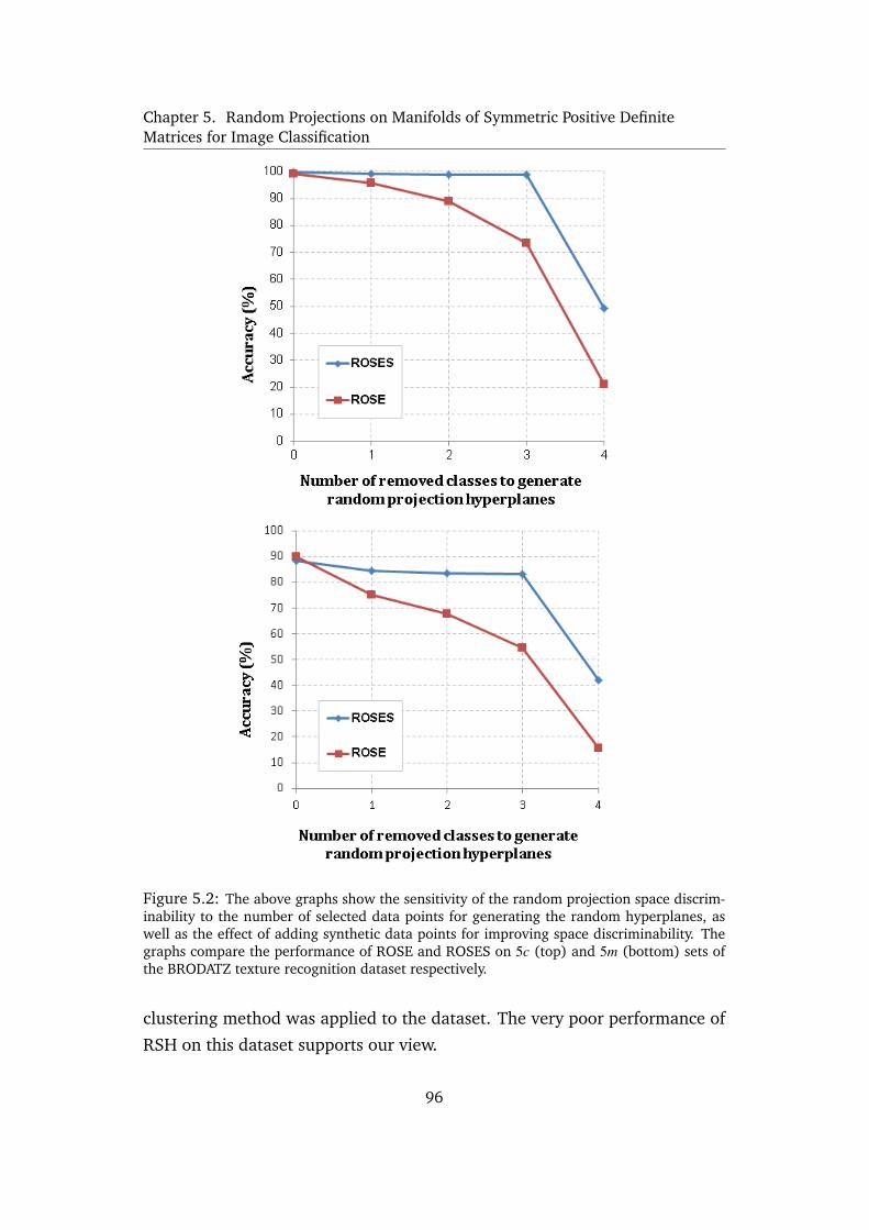
Chapter 5. Random Projections on Manifolds of Symmetric Positive DefiniteMatrices for Image Classification
Figure 5.2: The above graphs show the sensitivity of the random projection space discrim-inability to the number of selected data points for generating the random hyperplanes, aswell as the effect of adding synthetic data points for improving space discriminability. Thegraphs compare the performance of ROSE and ROSES on 5c (top) and 5m (bottom) sets ofthe BRODATZ texture recognition dataset respectively.
clustering method was applied to the dataset. The very poor performance of
RSH on this dataset supports our view.
96
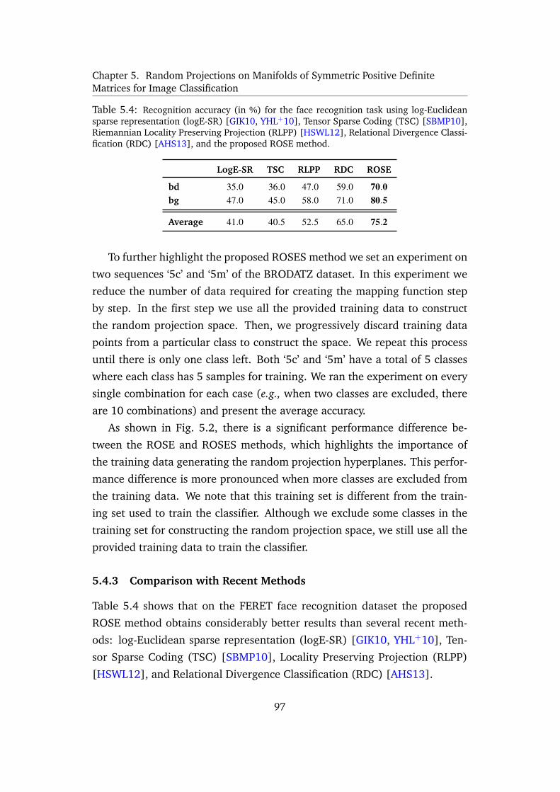
Chapter 5. Random Projections on Manifolds of Symmetric Positive DefiniteMatrices for Image Classification
Table 5.4: Recognition accuracy (in %) for the face recognition task using log-Euclideansparse representation (logE-SR) [GIK10, YHL+10], Tensor Sparse Coding (TSC) [SBMP10],Riemannian Locality Preserving Projection (RLPP) [HSWL12], Relational Divergence Classi-fication (RDC) [AHS13], and the proposed ROSE method.
LogE-SR TSC RLPP RDC ROSE
bd 35.0 36.0 47.0 59.0 70.0bg 47.0 45.0 58.0 71.0 80.5
Average 41.0 40.5 52.5 65.0 75.2
To further highlight the proposed ROSES method we set an experiment on
two sequences ‘5c’ and ‘5m’ of the BRODATZ dataset. In this experiment we
reduce the number of data required for creating the mapping function step
by step. In the first step we use all the provided training data to construct
the random projection space. Then, we progressively discard training data
points from a particular class to construct the space. We repeat this process
until there is only one class left. Both ‘5c’ and ‘5m’ have a total of 5 classes
where each class has 5 samples for training. We ran the experiment on every
single combination for each case (e.g., when two classes are excluded, there
are 10 combinations) and present the average accuracy.
As shown in Fig. 5.2, there is a significant performance difference be-
tween the ROSE and ROSES methods, which highlights the importance of
the training data generating the random projection hyperplanes. This perfor-
mance difference is more pronounced when more classes are excluded from
the training data. We note that this training set is different from the train-
ing set used to train the classifier. Although we exclude some classes in the
training set for constructing the random projection space, we still use all the
provided training data to train the classifier.
5.4.3 Comparison with Recent Methods
Table 5.4 shows that on the FERET face recognition dataset the proposed
ROSE method obtains considerably better results than several recent meth-
ods: log-Euclidean sparse representation (logE-SR) [GIK10, YHL+10], Ten-
sor Sparse Coding (TSC) [SBMP10], Locality Preserving Projection (RLPP)
[HSWL12], and Relational Divergence Classification (RDC) [AHS13].
97
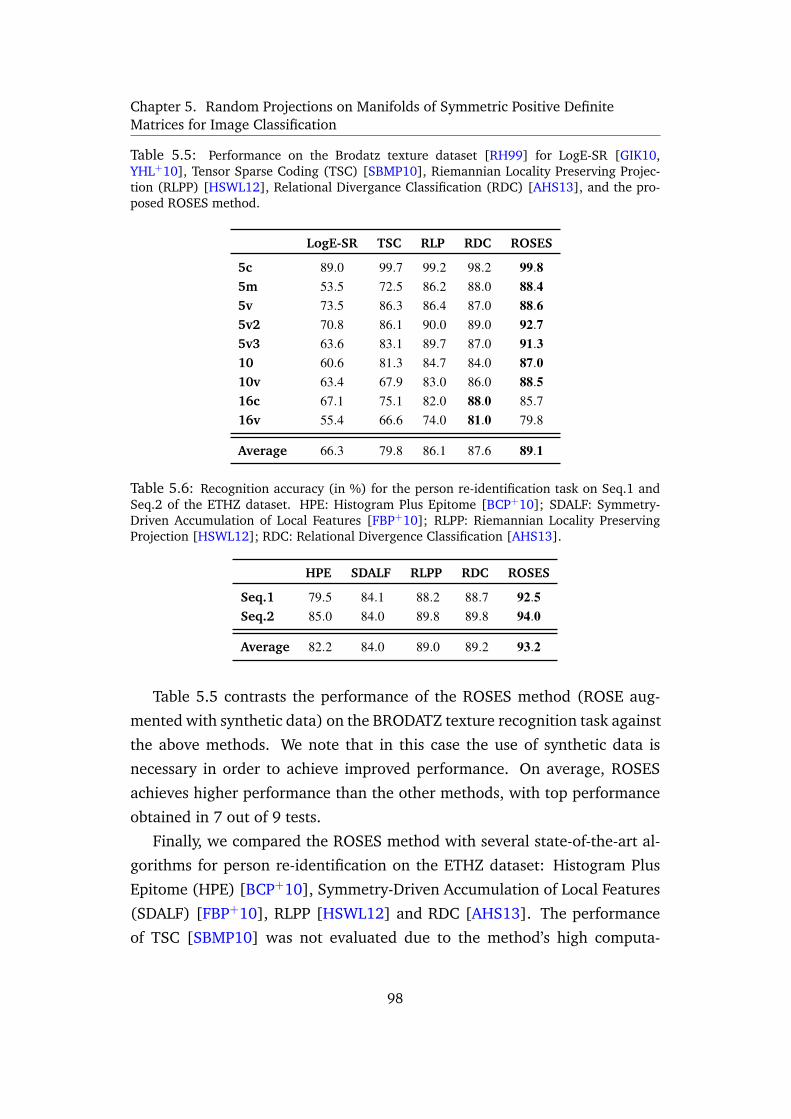
Chapter 5. Random Projections on Manifolds of Symmetric Positive DefiniteMatrices for Image Classification
Table 5.5: Performance on the Brodatz texture dataset [RH99] for LogE-SR [GIK10,YHL+10], Tensor Sparse Coding (TSC) [SBMP10], Riemannian Locality Preserving Projec-tion (RLPP) [HSWL12], Relational Divergance Classification (RDC) [AHS13], and the pro-posed ROSES method.
LogE-SR TSC RLP RDC ROSES
5c 89.0 99.7 99.2 98.2 99.85m 53.5 72.5 86.2 88.0 88.45v 73.5 86.3 86.4 87.0 88.65v2 70.8 86.1 90.0 89.0 92.75v3 63.6 83.1 89.7 87.0 91.310 60.6 81.3 84.7 84.0 87.010v 63.4 67.9 83.0 86.0 88.516c 67.1 75.1 82.0 88.0 85.716v 55.4 66.6 74.0 81.0 79.8
Average 66.3 79.8 86.1 87.6 89.1
Table 5.6: Recognition accuracy (in %) for the person re-identification task on Seq.1 andSeq.2 of the ETHZ dataset. HPE: Histogram Plus Epitome [BCP+10]; SDALF: Symmetry-Driven Accumulation of Local Features [FBP+10]; RLPP: Riemannian Locality PreservingProjection [HSWL12]; RDC: Relational Divergence Classification [AHS13].
HPE SDALF RLPP RDC ROSES
Seq.1 79.5 84.1 88.2 88.7 92.5Seq.2 85.0 84.0 89.8 89.8 94.0
Average 82.2 84.0 89.0 89.2 93.2
Table 5.5 contrasts the performance of the ROSES method (ROSE aug-
mented with synthetic data) on the BRODATZ texture recognition task against
the above methods. We note that in this case the use of synthetic data is
necessary in order to achieve improved performance. On average, ROSES
achieves higher performance than the other methods, with top performance
obtained in 7 out of 9 tests.
Finally, we compared the ROSES method with several state-of-the-art al-
gorithms for person re-identification on the ETHZ dataset: Histogram Plus
Epitome (HPE) [BCP+10], Symmetry-Driven Accumulation of Local Features
(SDALF) [FBP+10], RLPP [HSWL12] and RDC [AHS13]. The performance
of TSC [SBMP10] was not evaluated due to the method’s high computa-
98

Chapter 5. Random Projections on Manifolds of Symmetric Positive DefiniteMatrices for Image Classification
tional demands: it would take approximately 200 hours to process the ETHZ
dataset. We do not report the results for LogE-SR due to its low perfor-
mance on the other two datasets. The results shown in Table 5.6 indicate
that the proposed ROSES method obtains better performance. As in the pre-
vious experiment, the use of synthetic data is necessary to obtain improved
performance.
99
Chapter 6
Conclusion
This thesis contributes toward the improvement of visual analysis with the
aid of Symmetric Positive Definite(SPD) Manifolds. To be able to handle the
challenges of the real world environment, which are naturally not free from
noise, and in order to have a robust image descriptor, we have employed
covariance matrices to represent given scenes. The key advantage of repre-
senting images in forms of non-singular covariance matrices is that superior
performance can be achieved when the underlying structure of the group is
considered. It has been shown that when endowed with the Affine Invari-
ant Riemannian Metric (AIRM), the matrices form a connected, smooth and
differentiable Riemannian manifold.
However, as Non-singular covariance matrices are in form of SPD matri-
ces that form connected Riemannian manifolds, the Riemannian geometry is
required for solving learning tasks. Working directly on the manifold space
via AIRM poses many computational challenges.
Typical ways of addressing this issue include embedding the manifolds
to tangent spaces, and embedding into Reproducing Kernel Hilbert Spaces
(RKHS). Embedding the manifolds to tangent spaces considerably simplifies
further analysis, at the cost of disregarding some of the manifold structure.
Embedding via RKHS can better preserve the manifold structure, but adds the
burden of extending existing Euclidean-based learning algorithms into RKHS.
Riemannian manifolds address the limitations of using traditional methods,
while being mindful about the practicality of the method (for instance, en-
suring that the method is not computationally very complex).
100
Chapter 6. Conclusion
We make individual contributions to the following solutions on SPD man-
ifolds:
(i) Graph-Embedding Discriminant Analysis (ii) Relational Divergence
Based Classification (iii) Random Projection
For these solutions we propose novel approaches followed by a set of
designed experiments. In the following sections we summarise the contribu-
tions, possible extensions, and future research directions per algorithm.
6.1 Graph-Embedding Discriminant Analysis
In this work, we showed how discriminant analysis can be reformulated on
SPD manifolds. Inference on manifold spaces is generally achieved by em-
bedding the manifolds in higher dimensional Euclidean spaces, which can be
considered as flattening the manifolds. In this work we propose to embed
Riemannian manifolds into Reproducing Kernel Hilbert Spaces (RKHS). Em-
bedding a manifold into RKHS in turn opens the door for employing many
kernel-based machine learning algorithms [STC04]. As such, we tackle the
problem of Discriminant Analysis (DA) on Riemannian manifolds through
RKHS space and propose a graph-based local DA that utilises both within-
class and between-class similarity graphs to characterise intra-class compact-
ness and inter-class separability, respectively.
Thorough experiments on face and object recognition, action recogni-
tion, texture classification and person re-identification showed that notable
improvements in discrimination accuracy can be obtained through graph-
embedding analysis.
6.1.1 Future work
• Employing Stein Divergence instead of geodesic distance to make the
algorithm computationally more efficient.
• Investigate optimised parameter selection, as inappropriate parameter
selection might result in poor performance due to the structure of man-
ifold being encoded via the between and within similarity graphs.
101
Chapter 6. Conclusion
6.2 Relational Divergence Based Classification
The proposed method offers a new solution for analysing Riemannian man-
ifolds, where embedding into Euclidean spaces is not explicitly required. To
this end, we proposed to represent Riemannian points through their sim-
ilarities to a set of reference points on the manifold, with the aid of the
recently proposed Stein divergence, which is a symmetrised version of Breg-
man matrix divergence. Classification problems on manifolds are then effec-
tively converted into the problem of finding appropriate machinery over the
space of similarities, which can be tackled by conventional Euclidean learn-
ing methods such as linear discriminant analysis.
Experiments on face recognition, person reidentification and texture clas-
sification show that the proposed method outperforms state-of-the-art ap-
proaches, such as Tensor Sparse Coding, Histogram Plus Epitome, Rieman-
nian Locality Preserving Projection and log-Euclidean Sparse Representation.
6.2.1 Future work
• In the proposed approach we used all the training samples as reference
points (see Eqn. 4.12). While this approach is effective, more work is
required for selecting stronger set of reference points. This is because,
an optimized set of reference points can reduce the affect of outliers,
and result in reducing computational complexity.
• For classes with many examples, this approach may not be scalable. As
such, future avenues of research include defining alternative methods of
creating class representers, such as clustering directly on the manifold.
6.3 Random Projection
In this work, we have presented a novel solution which embeds the data
points into a random projection space by first generating random hyperplanes
in RKHS and then projecting the data in RKHS into the random projection
space. We presented a study of space discriminability for various computer
vision classification tasks and found that the random projection space has su-
102
Chapter 6. Conclusion
perior discriminative power in comparison to the typical approaches outlined
above. In addition, we found that the space discriminative power depends on
the completeness of the training data generating the random hyperplanes. To
address this issue, we proposed to augment the training data with synthetic
data.
Experiments on face recognition, person re-identification and texture clas-
sification show that the proposed method (combined with a linear SVM)
outperforms state-of-the-art approaches such as Tensor Sparse Coding, His-
togram Plus Epitome, Riemannian Locality Preserving Projection and Rela-
tional Divergence Classification. To our knowledge this is the first time ran-
dom projection space has been applied to solve classification tasks in mani-
fold space. We envision that the proposed method can be used to bring su-
perior discriminative power of manifold spaces to more general vision tasks,
such as object recognition and classification.
6.3.1 Future work
• The algorithm uses all the training data which makes it impractical for
very large datasets. Although for large datasets a random selection of
data can be used as a representor of the entire dataset, it would be
ideal to find an efficient data selection algorithm to replace the random
selection method.
• Inappropriate parameter selection might result in poor performance
which would be resolved by defining an effective optimisation formula.
6.4 Combining the proposed methods
To take advantage of all the proposed methods, one could benefit from using
a combination of the proposed methods. Below are a number of suggested
avenues for future work based on combining the methods detailed in this
thesis:
103

Chapter 6. Conclusion
6.4.1 Future work
• RDC uses distance matrix to calculate the similarity between a given
point and each class separately, then it employs LDA to classify given
points. On the other hand, ROSE uses random projection hyperplanes
in RKHS which, based on its randomness, does not necessarily generate
values that represent similarity of the given point to each class sepa-
rately. Being inspired by RDC method, one can employ RDC and con-
catenate its feature vector product with the feature vector computed by
ROSE to generate a more robust outcome that minimises the effect of
randomness.
• Similarly, inspired by RGDA, one can employ Graph-Embedding Dis-
criminant Analysis over a random projection space to improve the dis-
crimination power.
104
Appendix
In this section we provide more details to support the Proposition 5.3.3, thus
we show that for SPD matrices log(Xc) = c× log(X). For this proof we let c to
be a positive integer, however it is easy to extend the proof into real numbers.
log(Xc) = log(X×X× ...×X︸ ︷︷ ︸c
)
Replacing X with its Singular Value Decomposition (SVD) as X = U×V×U>,
the equation becomes:
log(X×X× ...×X︸ ︷︷ ︸c
) = log(U×V×U>×U×V×U>× ...×U×V×U>)
As X∈ Symd+ the eigenvalue matrix U is orthonormal, and therefore U>×U =
I. Hence, the below equation is valid:
log(Xc) = log(UVcU>)
Similarly, as X ∈ Symd+ therefore log(X) = U log(V) U> [TPM08].
log(Xc) = U log(Vc) U>
105

Appendix
where log(V) is the diagonal matrix of the eigenvalue logarithm [TPM08].
log(Xc) = U log(Vc) U>
= c U log(V) U>
= c× log(X)
106
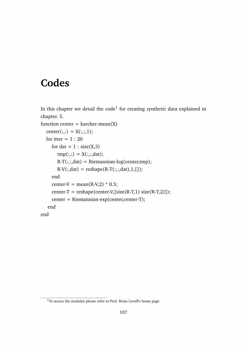
Codes
In this chapter we detail the code1 for creating synthetic data explained in
chapter. 5.
function center = karcher-mean(X)
center(:,:) = X(:,:,1);
for itter = 1 : 20
for dat = 1 : size(X,3)
tmp(:,:) = X(:,:,dat);
R-T(:,:,dat) = Riemannian-log(center,tmp);
R-V(:,dat) = reshape(R-T(:,:,dat),1,[]);
end
center-V = mean(R-V,2) * 0.5;
center-T = reshape(center-V,[size(R-T,1) size(R-T,2)]);
center = Riemannian-exp(center,center-T);
end
end
1To access the modules please refer to Prof. Brian Lovell’s home page
107

Codes
This function brings a point in riemannian manifold into a tangent space
T ×M where the point X coincides with the 0 in the tangent space Written by
the coauther Arnold Wiliem 2011.
function y = Riemannian-log(X,Y)
X05 = X0.5;
Xm05 = X−0.5;
temp = Xm05*Y*Xm05;
[V,D] = eig(temp);
logTemp = V * diag(diag(log(D))) * V’;
y = X05* logTemp * X05;
end
108

Codes
This function brings a point in a tangent space T ×M where the point X
coincides with the 0 into the manifold. This part is written by the co-author
Arnold Wiliem on 2011.
function Y = Riemannian-exp(X,y)
X05 = X0.5;
Xm05 = X−0.5;
temp = Xm05*y*Xm05;
[V,D] = eig(temp);
expTemp = V * diag(diag(exp(D))) * V’;
Y = X05* expTemp * X05;
end
109

Codes
This function uses all the above functions to compute the synthetic data
on Riemannian manifold
Center = Karcher-Mean(Training-Data);
for i = 1 : number-of-Samples
tmp = cov(randn(100,Dimension));
tmp = tmp + diag(diag(tmp));
X(:,:) = Center;
if (∑(eig(tmp) 0) 0)
eig(tmp)
break;
end
dist- = Riemannian-GeodesicDist(X,tmp);
tngnt-pnt = Riemannian-log(X,tmp);
tngnt-pnt = (tngnt-pnt ./ dist-) * theta(cnt-cnt) * rand;
pnt(:,:,i) = Riemannian-exp(X,tngnt-pnt);
end
110
Bibliography
[Ach03] D. Achlioptas. Database-friendly random projections: Johnson-
lindenstrauss with binary coins. Journal of Computer and SystemSciences, 66(4):671–687, 2003.
[AHS13] A. Alavi, M. T. Harandi, and C. Sanderson. Relational divergence
based classification on Riemannian manifolds. In IEEE Work-shop on Applications of Computer Vision (WACV), pages 111–116,
2013.
[AMP09] A. Argyriou, C. A. Micchelli, and M. Pontil. When is there a rep-
resenter theorem? Vector versus matrix regularizers. Journal ofMachine Learning Research, 10:2507–2529, December 2009.
[AMU97] Y. Adini, Y. Moses, and S. Ullman. Face recognition: the
problem of compensating for changes in illumination direction.
IEEE Transactions on Pattern Analysis and Machine Intelligence,
19(7):721 –732, 1997.
[AR05] T. Acharya and A. K. Ray. Image Processing: Principles and Appli-cations. 2005.
[ASHL13] A. Alavi, S. Shirazi, M. T. Harandi, and B. C. Lovell. Graph-
embedding discriminant analysis on Riemannian manifolds for
visual recognition. In Graph Embedding for Pattern Analysis, pages
157–175. Springer, 2013.
[AVN11] C. Anoop, M. Vassilios, and P. Nikolaos. Dirichlet process mixture
models on symmetric positive definite matrices for appearance
clustering in video surveillance applications. In IEEE Conf. Com-
111
Bibliography
puter Vision and Pattern Recognition (CVPR), pages 3417–3424,
2011.
[AYHS13] A. Alavi, Y. Yang, M. Harandi, and C. Sanderson. Multi-shot per-
son re-identification via relational Stein divergence. 2013.
[BCBTss] S. Bak, E. Corve, F. Brmond, and M. Thonnat. Boosted human
re-identification using Riemannian manifolds. Image and VisionComputing, (0):–, in press.
[BCP+10] L. Bazzani, M. Cristani, A. Perina, M. Farenzena, and V. Murino.
Multiple-shot person re-identification by HPE signature. In Pro-ceedings of the 2010 20th International Conference on PatternRecognition, pages 1413–1416. IEEE Computer Society, 2010.
[BHK97] P. Belhumeur, J. Hespanha, and D. Kriegman. Eigenfaces vs.
fisherfaces: Recognition using class specific linear projection.
IEEE Transactions on Pattern Analysis and Machine Intelligence,
19(7):711–720, 1997.
[Bis06] C. M. Bishop. Pattern Recognition and Machine Learning. Springer,
2006.
[CGG+09] Y. Chen, E. K. Garcia, M. R. Gupta, A. Rahimi, and L. Cazzanti.
Similarity-based classification: Concepts and algorithms. Journalof Machine Learning Research, 10:747–776, 2009.
[Cha02] M. S. Charikar. Similarity estimation techniques from rounding
algorithms. In Proceedings of the thiry-fourth annual ACM sympo-sium on Theory of Computing, pages 380–388. ACM, 2002.
[Che12] R. Chellappa. Introduction. Image and Vision Computing, 30:379,
2012.
[CI10] R. Chaudhry and Y. Ivanov. Fast approximate nearest neighbor
methods for non-Euclidean manifolds with applications to human
activity analysis in videos. In The 11th European Conference onComputer Vision, pages 735–748. Springer-Verlag, 2010.
112
Bibliography
[CM02] D. Comaniciu and P. Meer. Mean shift: A robust approach toward
feature space analysis. IEEE Trans. Pattern Analysis and MachineIntelligence, 24(5):603–619, 2002.
[CSBP11] A. Cherian, S. Sra, A. Banerjee, and N. Papanikolopoulos. Ef-
ficient similarity search for covariance matrices via the Jensen-
Bregman LogDet divergence. In International Conference on Com-puter Vision (ICCV), pages 2399–2406, 2011.
[CT10] H. Cevikalp and B. Triggs. Face recognition based on image sets.
In IEEE Conference on Computer Vision and Pattern Recognition(CVPR), pages 2567–2573. IEEE, 2010.
[DC11] G. F. T. Del Castillo. Differentiable Manifolds: A Theoretical PhysicsApproach. Springer, 2011.
[DIIM04] M. Datar, N. Immorlica, P. Indyk, and V. S. Mirrokni. Locality-
sensitive hashing scheme based on p-stable distributions. In Pro-ceedings of the twentieth annual symposium on Computational Ge-ometry, pages 253–262. ACM, 2004.
[EAS99] A. Edelman, T. A. Arias, and S. T. Smith. The geometry of al-
gorithms with orthogonality constraints. SIAM Journal MatrixAnalysis and Application, 20(2):303–353, 1999.
[ELG07] A. Ess, B. Leibe, and L. V. Gool. Depth and appearance for mo-
bile scene analysis. International Conference on Computer Vision(ICCV), pages 1–8, 2007.
[FBP+10] M. Farenzena, L. Bazzani, A. Perina, V. Murino, and M. Cristani.
Person re-identification by symmetry-driven accumulation of lo-
cal features. In Computer Vision and Pattern Recognition (CVPR),2010 IEEE Conference on, pages 2360–2367. IEEE, 2010.
[FCH+08] R.-E. Fan, K.-W. Chang, C.-J. Hsieh, X.-R. Wang, and C.-J. Lin.
LIBLINEAR: A library for large linear classification. Journal ofMachine Learning Research, 9:1871–1874, 2008.
113
Bibliography
[FGR05] M. Foracchia, E. Grisan, and A. Ruggeri. Luminosity and con-
trast normalization in retinal images. Medical Image Analysis,9(3):179–190, 2005.
[GBT07a] D. Gray, S. Brennan, and H. Tao. Evaluating appearance mod-
els for recognition, reacquisition, and tracking. In IEEE Inter-national Workshop on Performance Evaluation for Tracking andSurveillance, 2007.
[GBT07b] D. Gray, S. Brennan, and H. Tao. Evaluating appearance mod-
els for recognition, reacquisition, and tracking. In In Proceedingsof the IEEE International Workshop on Performance Evaluation forTracking and Surveillance (PETS), volume 3, page 5, 2007.
[GIK10] K. Guo, P. Ishwar, and J. Konrad. Action recognition using sparse
representation on covariance manifolds of optical flow. In IEEEConf. Advanced Video and Signal Based Surveillance (AVSS), pages
188–195, 2010.
[GK86] P. Geladi and B. Kowalski. Partial least-squares regression: a tu-
torial. Analytica Chimica Acta, 185:1–17, 1986.
[GT08] D. Gray and H. Tao. Viewpoint invariant pedestrian recognition
with an ensemble of localized features. In Computer Vision–ECCV2008, Lecture Notes in Computer Science, volume 5302, pages
262–275, 2008.
[HL08] J. Hamm and D. D. Lee. Grassmann discriminant analysis: a
unifying view on subspace-based learning. In International Con-ference on Machine Learning (ICML), pages 376–383, 2008.
[HL09] J. Hamm and D. D. Lee. Extended Grassmann kernels for
subspace-based learning. In D. Koller, D. Schuurmans, Y. Bengio,
and L. Bottou, editors, Advances in Neural Information ProcessingSystems (NIPS), pages 601–608. 2009.
[HLL+ss] W. Hu, X. Li, W. Luo, X. Zhang, S. Maybank, and Z. Zhang. Sin-
gle and multiple object tracking using log-Euclidean Riemannian
114
Bibliography
subspace and block-division appearance model. IEEE Trans. Pat-tern Analysis and Machine Intelligence, in press.
[HSHL12] M. T. Harandi, C. Sanderson, R. Hartley, and B. C. Lovell. Sparse
coding and dictionary learning for symmetric positive definite
matrices: A kernel approach. In European Conference on Com-puter Vision (ECCV), Lecture Notes in Computer Science (LNCS),
volume 7573, pages 216–229, 2012.
[HSSL11] M. T. Harandi, C. Sanderson, S. Shirazi, and B. C. Lovell. Graph
embedding discriminant analysis on Grassmannian manifolds for
improved image set matching. In IEEE Conference on ComputerVision and Pattern Recognition (CVPR), pages 2705–2712, 2011.
[HSWL12] M. Harandi, C. Sanderson, A. Wiliem, and B. Lovell. Kernel anal-
ysis over Riemannian manifolds for visual recognition of actions,
pedestrians and textures. IEEE Workshop on the Applications ofComputer Vision (WACV), pages 433–439, 2012.
[JA10] K. Jungling and M. Arens. Local feature based person reiden-
tification in infrared image sequences. In Seventh IEEE Interna-tional Conference on Advanced Video and Signal Based Surveillance(AVSS), pages 448–455. IEEE, 2010.
[Jam99] I. M. James. History of Topology. Access Online via Elsevier, 1999.
[JFK03] N. Jojic, B. J. Frey, and A. Kannan. Epitomic analysis of appear-
ance and shape. IEEE International Conference on Computer Vi-sion, 1:34–41, 2003.
[JKG08] P. Jain, B. Kulis, and K. Grauman. Fast image search for learned
metrics. In IEEE Conference on Computer Vision and Pattern Recog-nition (CVPR), pages 1–8. IEEE, 2008.
[JPC+09] N. Jojic, A. Perina, M. Cristani, V. Murino, and B. Frey. STEL
component analysis: Modeling spatial correlations in image class
structure. In IEEE Conference on Computer Vision and PatternRecognition, pages 2044–2051, 2009.
115
Bibliography
[KG09] B. Kulis and K. Grauman. Kernelized locality-sensitive hashing for
scalable image search. In International Conference on ComputerVision, pages 2130–2137. IEEE, 2009.
[KW70] G. S. Kimeldorf and G. Wahba. A correspondence between
bayesian estimation on stochastic processes and smoothing by
splines. The Annals of Mathematical Statistics, 41:495–502, 1970.
[Lan99] S. Lang. Fundamentals of Differential Geometry, volume 160.
Springer Verlag, 1999.
[Lee96] T. Lee. Image representation using 2D Gabor wavelets. Pat-tern Analysis and Machine Intelligence, IEEE Transactions on,
18(10):959–971, 1996.
[Lee97] J. M. Lee. Riemannian manifolds: an introduction to curvature,
volume 176. Springer, 1997.
[LTSC13] R. Li, P. Turaga, A. Srivastava, and R. Chellappa. Differential ge-
ometric representations and algorithms for some pattern recog-
nition and computer vision problems. Pattern Recognition Letters,2013.
[Lui11] Y. Lui. Tangent bundles on special manifolds for action recog-
nition. IEEE Trans. Circuits and Systems for Video Technology,
22(6):930–942, 2011.
[Lui12] Y. M. Lui. Advances in matrix manifolds for computer vision.
Image and Vision Computing, 30(6):380–388, 2012.
[OLDss] S. O’Hara, Y. M. Lui, and B. A. Draper. Using a product manifold
distance for unsupervised action recognition. Image and VisionComputing, 2012 (in press).
[Pen06] X. Pennec. Intrinsic statistics on Riemannian manifolds: Basic
tools for geometric measurements. Journal of Mathematical Imag-ing and Vision, 25(1):127–154, 2006.
116
Bibliography
[PFA06] X. Pennec, P. Fillard, and N. Ayache. A riemannian framework
for tensor computing. International Journal of Computer Vision,
66(1):41–66, 2006.
[PMRR00] P. Phillips, H. Moon, S. Rizvi, and P. Rauss. The FERET evaluation
methodology for face-recognition algorithms. IEEE Transactionson Pattern Analysis and Machine Intelligence, 22(10):1090–1104,
2000.
[PTM06] F. Porikli, O. Tuzel, and P. Meer. Covariance tracking using model
update based on Lie algebra. In IEEE Conf. Computer Vision andPattern Recognition (CVPR), pages 728–735, 2006.
[PYL08] Y. Pang, Y. Yuan, and X. Li. Gabor-based region covariance matri-
ces for face recognition. IEEE Transactions on Circuits and Systemsfor Video Technology, 18(7):989–993, 2008.
[RH99] T. Randen and J. Husoy. Filtering for texture classification: A
comparative study. Pattern Analysis and Machine Intelligence, IEEETransactions on, 21(4):291–310, 1999.
[Ric07] J. A. Rice. Mathematical statistics and data analysis. Cengage
Learning, 2007.
[Ros97] S. Rosenberg. The Laplacian on a Riemannian Manifold: An In-troduction to Analysis on Manifolds. Cambridge University Press,
1997.
[RS00] S. T. Roweis and L. K. Saul. Nonlinear dimensionality reduc-
tion by locally linear embedding. Science, 290(5500):2323–2326,
2000.
[RSL13] V. Reddy, C. Sanderson, and B. C. Lovell. Improved foreground
detection via block-based classifier cascade with probabilistic de-
cision integration. IEEE Transactions on Circuits and Systems forVideo Technology, 23(1):83–93, 2013.
[SA11] S. Suvrit and C. Anoop. Generalized dictionary learning for
symmetric positive definite matrices with application to near-
117

Bibliography
est neighbor retrieval. European Conference on Machine Learning(ECML), 2011.
[SBMP10] R. Sivalingam, D. Boley, V. Morellas, and N. Papanikolopoulos.
Tensor sparse coding for region covariances. In European Confer-ence on Computer Vision (ECCV), volume 6314 of Lecture Notes inComputer Science, pages 722–735. 2010.
[SC11] S. Sra and A. Cherian. Generalized dictionary learning for
symmetric positive definite matrices with application to nearest
neighbor retrieval. In Machine Learning and Knowledge Discoveryin Databases, pages 318–332. Springer, 2011.
[SD09] W. Schwartz and L. Davis. Learning discriminative appearance-
based models using partial least squares. In Computer Graphicsand Image Processing (SIBGRAPI), pages 322–329. IEEE, 2009.
[SL00] H. S. Seung and D. D. Lee. The manifold ways of perception.
Science, 290(5500):2268–2269, 2000.
[SM09] R. Subbarao and P. Meer. Nonlinear mean shift over Riemannian
manifolds. Int. J. Computer Vision, 84(1):1–20, 2009.
[Sra12] S. Sra. Positive definite matrices and the symmetric Stein diver-
gence. Preprint: [arXiv:1110.1773], 2012.
[SSHH12] Q. Shi, C. Shen, R. Hill, and A. v. d. Hengel. Is margin preserved
after random projection? ICML, 2012.
[STC04] J. Shawe-Taylor and N. Cristianini. Kernel Methods for PatternAnalysis. Cambridge University Press, 2004.
[TA77] A. N. Tikhonov and V. Y. Arsenin. Solutions of Ill-Posed Problems.V. H. Winston & Sons, Washington, D.C.: John Wiley & Sons,
New York, 1977.
[TDSL00] J. B. Tenenbaum, V. De Silva, and J. C. Langford. A global ge-
ometric framework for nonlinear dimensionality reduction. Sci-ence, 290(5500):2319–2323, 2000.
118
Bibliography
[TP91] M. Turk and A. Pentland. Eigenfaces for recognition. Journal ofCognitive Neuroscience, 3(1):71–86, 1991.
[TPM06a] O. Tuzel, F. Porikli, and P. Meer. Region covariance: A fast de-
scriptor for detection and classification. In Computer Vision–ECCV2006, pages 589–600. Springer, 2006.
[TPM06b] O. Tuzel, F. Porikli, and P. Meer. Region covariance: A fast
descriptor for detection and classification. In A. Leonardis,
H. Bischof, and A. Pinz, editors, European Conference on Com-puter Vision (ECCV), volume 3952 of Lecture Notes in ComputerScience, pages 589–600. Springer Berlin / Heidelberg, 2006.
[TPM08] O. Tuzel, F. Porikli, and P. Meer. Pedestrian detection via classi-
fication on Riemannian manifolds. IEEE Transactions on PatternAnalysis and Machine Intelligence (PAMI), 30:1713–1727, October
2008.
[TVC08] P. Turaga, A. Veeraraghavan, and R. Chellappa. Statistical analy-
sis on Stiefel and Grassmann manifolds with applications in com-
puter vision. In Computer Vision and Pattern Recognition (CVPR),
pages 1–8. IEEE, 2008.
[TVSC11] P. Turaga, A. Veeraraghavan, A. Srivastava, and R. Chellappa.
Statistical computations on Grassmann and Stiefel manifolds for
image and video-based recognition. Pattern Analysis and MachineIntelligence, IEEE Transactions on, 33(11):2273–2286, 2011.
[VRCC05] A. Veeraraghavan, A. Roy-Chowdhury, and R. Chellappa. Match-
ing shape sequences in video with applications in human
movement analysis. Pattern Analysis and Machine Intelligence,
27(12):1896–1909, 2005.
[WKJ85] H. Wold, S. Kotz, and N. Johnson. Partial least squares. Encyclo-pedia of Statistical Sciences, 6:581–591, 1985.
[WS03] L. Wolf and A. Shashua. Learning over sets using kernel principal
angles. The Journal of Machine Learning Research, 4:913–931,
2003.
119

Bibliography
[YF08] J. Yeh and J. Fu. A hierarchical genetic algorithm for segmen-
tation of multi-spectral human-brain MRI. Expert Systems withApplications, 34(2):1285–1295, 2008.
[YHL+10] C. Yuan, W. Hu, X. Li, S. Maybank, and G. Luo. Human action
recognition under log-euclidean Riemannian metric. In AsianConference on Computer Vision (ACCV), volume 5994 of LectureNotes in Computer Science, pages 343–353. Springer Berlin / Hei-
delberg, 2010.
[ZGX09] W. Zheng, S. Gong, and T. Xiang. Associating groups of people.
In British Machine Vision Conference, volume 1, pages 1–11, 2009.
120


![Part 1 - Université libre de Bruxellesscmero.ulb.ac.be/Teaching/Courses/MECA-H-411/MECA-H-411-Slides.… · = energy spectrum of f(t) 15. ... Symmetric & semi positive definite []](https://static.fdocuments.net/doc/165x107/5adb96187f8b9a4a268b8632/part-1-universit-libre-de-energy-spectrum-of-ft-15-symmetric-semi-positive.jpg)


![2.4 SOLVING SYSTEMS OF LINEAR EQUATIONSanitescu/CLASSES/2012/LECTURES/S310-2012-lect3.pdfCholesky LU Factorization • If [A] is symmetric and positive definite, it is convenient to](https://static.fdocuments.net/doc/165x107/5e5650aa114d8d26cc1c69c9/24-solving-systems-of-linear-equations-anitescuclasses2012lecturess310-2012-lect3pdf.jpg)
