Image analysis aided by Segmentation algorithms for...
12
Image analysis aided by Segmentation algorithms for techniques ranging from Scanning Probe Microscopy to Optical Microscopy M. D'Acunto, and O. Salvetti National Research Council, Istitute of Information Science and Technologies, ISTI-CNR, Via Moruzzi 1, 54124, Pisa,Italy [email protected] ; [email protected] Microscope image analysis is a common term that covers the use of digital image processing techniques to process and analyse images obtained with all the range of available microscopes, ranging from the Scanning Probe Microscopy (SPM) family, operating down to atomic scale, to Optical Microscopy (OM). Such processing techniques are now commonplace in a number of different fields such as medicine, biology, physics, chemistry, engineering. As a consequence, a number of manufacturers of microscopes now specifically design in features that allow the microscopes to interface to an image processing tool. Nevertheless, in many applications where a rough image analysis is requested, image processing systems are not enough for corrections of specific instrumental distortions or for the correct recognition of unknown sample features. In this chapter, we describe the fundamental aid offered by segmentation techniques for image analysis of microscopes operating on different scales. Several segmentation algorithms are described and commented looking how they work when applied to various scale lengths. Keywords Image analysis; Denoising; Thresholding; Segmentation algorithms; Scanning Probe Microscopy; Optical Microscopy 1. Introduction Image processing applied to microscopy is a broad term that covers the use of digital image processing techniques to process, analyze and present images obtained from a microscope. Because microscopy is the technical field of using microscopes to view samples or objects that cannot be seen with the unaided eye collecting images (imaging), the processing techniques for manipulating data stored in the images are the main challenging problems. There are three well-known branches of microscopy, optical, electron and scanning probe microscopy. Any of such techniques employs physical and instrumental mechanisms that produce a priori known artefacts and unknown features that have to be carefully removed to acquire meaningful information from the recorded images. For example, removing noise is a common pre-processing procedure to be applied in all the microscopy techniques. Thus common thresholding, edge detection and segmentation techniques can be applied to distinguish between the objects of interest and the background. Optical and electron microscopy involve the diffraction, reflection, or refraction of electromagnetic radiation or electron beams interacting with the subject of study, and the subsequent collection of this scattered radiation in order to build up an image. This process may be carried out by wide-field irradiation of the sample, as in the standard light OM or the Transmission Electron Microscopy (TEM). An alternative is represented by scanning of a fine beam over the sample, as in the Confocal Laser Scanning Microscopy (CLSM) and Scanning Electron Microscopy (SEM). In turn, SPM involves the interaction of a scanning probe with the surface or object of interest. An image of the surface is obtained by mechanically moving the probe in a raster scan of the specimen, line by line, and recording the probe –surface interaction as a function of position. Many SPMs can image several interactions simultaneously. Within the SPM family, the resolution varies somewhat from technique to technique, but some probe techniques reach a true atomic resolution, based on the ability of piezoelectric attractors to execute motions with a precision and accuracy at the atomic level. In this chapter, we present a review of the some methods for pre-processing image analysis, denoising and thresholding, and some common segmentation technique focusing the attention on the basic principles and their aid on microscopy image principally on biomedical samples, such as cells. The chapter is organized as follows: the next section describes the most common image segmentation techniques. The section 3 is focused on some applications of the segmentation techniques to biological samples, for a wide range of microscopy techniques (OM, SEM, CLSM, AFM, etc.) stressing how the object recognition and identification is strongly enhanced by the application of segmentation. Finally, in the section 4, segmentation techniques united to pattern matching are used to face the problem of thermal drift in a sequence of image recorded with AFM and Force Modulation Microscope (FMM). 2. Image Segmentation Techniques, Denosing and Thresholding. An overview. Image segmentation is a procedure that partitions an image into disjointing groups with each group sharing similar properties such as intensity, color, boundary and texture. In general, three main image features are used to guide image segmentation, which are intensity or color, edge, and texture. In other words, image segmentation methods generally Microscopy: Science, Technology, Applications and Education A. Méndez-Vilas and J. Díaz (Eds.) ©FORMATEX 2010 1455 ______________________________________________
Transcript of Image analysis aided by Segmentation algorithms for...

Image analysis aided by Segmentation algorithms for techniques ranging
from Scanning Probe Microscopy to Optical Microscopy
M. D'Acunto, and O. Salvetti
National Research Council, Istitute of Information Science and Technologies, ISTI-CNR, Via Moruzzi 1, 54124, Pisa,Italy
[email protected]; [email protected]
Microscope image analysis is a common term that covers the use of digital image processing techniques to process and
analyse images obtained with all the range of available microscopes, ranging from the Scanning Probe Microscopy (SPM)
family, operating down to atomic scale, to Optical Microscopy (OM). Such processing techniques are now commonplace
in a number of different fields such as medicine, biology, physics, chemistry, engineering. As a consequence, a number of
manufacturers of microscopes now specifically design in features that allow the microscopes to interface to an image
processing tool. Nevertheless, in many applications where a rough image analysis is requested, image processing systems
are not enough for corrections of specific instrumental distortions or for the correct recognition of unknown sample
features. In this chapter, we describe the fundamental aid offered by segmentation techniques for image analysis of
microscopes operating on different scales. Several segmentation algorithms are described and commented looking how
they work when applied to various scale lengths.
Keywords Image analysis; Denoising; Thresholding; Segmentation algorithms; Scanning Probe Microscopy; Optical
Microscopy
1. Introduction
Image processing applied to microscopy is a broad term that covers the use of digital image processing techniques to
process, analyze and present images obtained from a microscope. Because microscopy is the technical field of using
microscopes to view samples or objects that cannot be seen with the unaided eye collecting images (imaging), the
processing techniques for manipulating data stored in the images are the main challenging problems. There are three
well-known branches of microscopy, optical, electron and scanning probe microscopy. Any of such techniques employs
physical and instrumental mechanisms that produce a priori known artefacts and unknown features that have to be
carefully removed to acquire meaningful information from the recorded images. For example, removing noise is a
common pre-processing procedure to be applied in all the microscopy techniques. Thus common thresholding, edge
detection and segmentation techniques can be applied to distinguish between the objects of interest and the background.
Optical and electron microscopy involve the diffraction, reflection, or refraction of electromagnetic radiation or electron
beams interacting with the subject of study, and the subsequent collection of this scattered radiation in order to build up
an image. This process may be carried out by wide-field irradiation of the sample, as in the standard light OM or the
Transmission Electron Microscopy (TEM). An alternative is represented by scanning of a fine beam over the sample, as
in the Confocal Laser Scanning Microscopy (CLSM) and Scanning Electron Microscopy (SEM). In turn, SPM involves
the interaction of a scanning probe with the surface or object of interest. An image of the surface is obtained by
mechanically moving the probe in a raster scan of the specimen, line by line, and recording the probe –surface
interaction as a function of position. Many SPMs can image several interactions simultaneously. Within the SPM
family, the resolution varies somewhat from technique to technique, but some probe techniques reach a true atomic
resolution, based on the ability of piezoelectric attractors to execute motions with a precision and accuracy at the atomic
level.
In this chapter, we present a review of the some methods for pre-processing image analysis, denoising and
thresholding, and some common segmentation technique focusing the attention on the basic principles and their aid on
microscopy image principally on biomedical samples, such as cells. The chapter is organized as follows: the next
section describes the most common image segmentation techniques. The section 3 is focused on some applications of
the segmentation techniques to biological samples, for a wide range of microscopy techniques (OM, SEM, CLSM,
AFM, etc.) stressing how the object recognition and identification is strongly enhanced by the application of
segmentation. Finally, in the section 4, segmentation techniques united to pattern matching are used to face the problem
of thermal drift in a sequence of image recorded with AFM and Force Modulation Microscope (FMM).
2. Image Segmentation Techniques, Denosing and Thresholding. An overview.
Image segmentation is a procedure that partitions an image into disjointing groups with each group sharing similar
properties such as intensity, color, boundary and texture. In general, three main image features are used to guide image
segmentation, which are intensity or color, edge, and texture. In other words, image segmentation methods generally
Microscopy: Science, Technology, Applications and Education A. Méndez-Vilas and J. Díaz (Eds.)
©FORMATEX 2010 1455
______________________________________________

fall into three main categories: color-based, edge-based, and texture-based segmentations. Color-based (or intensity-
based) segmentation assumes that an image is composed by several objects with constant intensity. This kind of
methods usually depends on intensity similarity comparisons to separate different objects. Histogram thresholding [1,
2], clustering [3, 4] and split-and-merge [5, 6], are typical examples of intensity-based segmentation methods. Edge-
based segmentation has a strong relationship with color-based segmentation, since edge usually indicate discontinuites
in image intensity. Widely used methods in edge-based segmentation include Canny [7], watershed [8], and snake [9,
10]. Texture is another important characteristic used to segment objects from background. Most texture-based
segmentation algorithms map an image into a texture feature space, then statistical classifications methods are used to
segment different texture features [11]. Co-occurrence matrix [12], directional gray-level energy [13], Gabor filters
[14], and fractal dimensions [15, 16], are frequently used methods to obtain texture features. Besides intensity, color,
contour and texture: object density is another attribute to be used when image analysis is requested to find appropriate
features on microscope measurements. For instance, in pathological tissue images, pathological diagnosis relies on
accurate separation of different cells [17-20].
The goal of image denoising methods is to recover the original image from a noisy measurement
)()()( iniuiv += (1)
where v(i) is the observed value, u(i) is the true value and n(i) is the noise perturbation at a pixel i. The best simple way
to model the effect of noise on a digital image is to add a Gaussian white noise. In this case, n(i) are gaussian value with
zero mean and variance σ2. Several methods have been proposed to remove the noise and recover the true image u.
Even through they may be very different in tools it must be emphasized that a wide class shares the same basic remark:
denoising is achieved by averaging. This averaging may be performed locally using Gaussian smoothing models [21],
or by the calculus of variations [22], or in the frequency domain: using empirical Wiener filters [23] or wavelet
thresholding methods [24]. Usually the denoising method is a decomposition technque Dh:
v=Dhv+n(Dh,v) (2)
where v is the observed value and h is the filtering parameter which generally depends on the standard deviation of the
noise. Ideally, Dhv is smoother than v and n(Dh,v) looks like the realization of a white noise. The decomposition of an
image between a smooth part and a non smooth or oscillatory part is a current subject of research [25]. The denoising
methods should not alter the original image u, unfortunately, most denoising methods degrade or remove the fine details
and texture of u. To avoid this unwanted consequence, it is necessary to minimize the function that accounts the
difference between the original (always slightly noisy) image u and its denoised version. Furthenmore, some denoising
methods can be comparised looking how they work on some microscopy images. We introduce some denoising
methods and we apply them to cell images, figures 1 and 2.
Let u be an image and Dh a denoising operator depending on a filtering parameter h. Then, we define the method
noise as the image difference
u-Dhu (3)
In a Gaussian filtering, the image isotropic linear filtering boils down to the convolution of the image by a linear
symmetric kernel:22
4/
24
1)(
hh e
hG
xx
−=π
so that the Eq. (3) becomes
( )22 houhuGu h +∆−=∗− (4)
where ∗ denotes convolution, ∆ is a Laplacian operator and for h small enough. The Gaussian method noise is zero in
harmonic parts of the image and very large near edges or texture, where the Laplacian cannot be small. As a
consequence, the Gaussian convolution is optimal in flat parts of the image but edges and texture are blurred. In
addition, neighbourhood averaging can suppress isolated out-of-range noise, but the side effect is that it also blurs
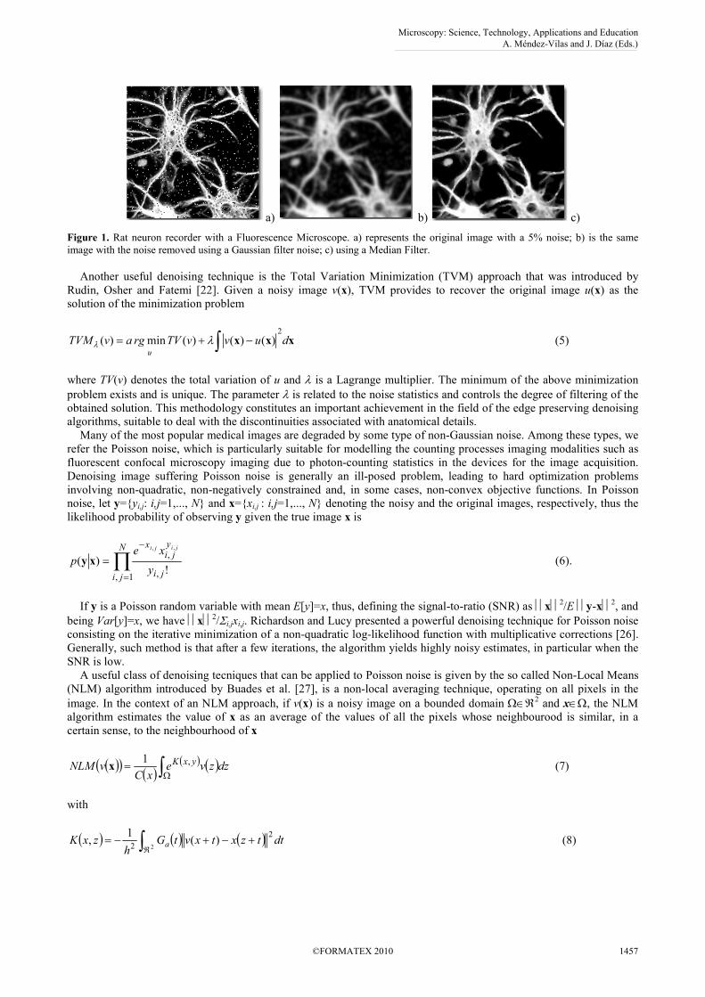
sudden changes (corresponding to high spatial frequencies) such as sharp edges. The Median Filter (MF) is an effective
method that can suppress isolated noise without blurring sharp edges. Specifically, the MF replaces a pixel by the
median of all pixels in the neighbourhood. A comparison between a Gaussian filter noise and a MF applied to a
Fluorescence Microscopy image of rat neurons is shown in figure 1.
Microscopy: Science, Technology, Applications and Education A. Méndez-Vilas and J. Díaz (Eds.)
1456 ©FORMATEX 2010
______________________________________________
a) b) c)
Figure 1. Rat neuron recorder with a Fluorescence Microscope. a) represents the original image with a 5% noise; b) is the same
image with the noise removed using a Gaussian filter noise; c) using a Median Filter.
Another useful denoising technique is the Total Variation Minimization (TVM) approach that was introduced by
Rudin, Osher and Fatemi [22]. Given a noisy image v(x), TVM provides to recover the original image u(x) as the
solution of the minimization problem
xxx duvvTVrgavTVMu
2
)()()(min)( ∫ −+= λλ (5)
where TV(v) denotes the total variation of u and λ is a Lagrange multiplier. The minimum of the above minimization
problem exists and is unique. The parameter λ is related to the noise statistics and controls the degree of filtering of the obtained solution. This methodology constitutes an important achievement in the field of the edge preserving denoising
algorithms, suitable to deal with the discontinuities associated with anatomical details.
Many of the most popular medical images are degraded by some type of non-Gaussian noise. Among these types, we
refer the Poisson noise, which is particularly suitable for modelling the counting processes imaging modalities such as
fluorescent confocal microscopy imaging due to photon-counting statistics in the devices for the image acquisition.
Denoising image suffering Poisson noise is generally an ill-posed problem, leading to hard optimization problems
involving non-quadratic, non-negatively constrained and, in some cases, non-convex objective functions. In Poisson
noise, let y=yi,j: i,j=1,..., N and x=xi,j : i,j=1,..., N denoting the noisy and the original images, respectively, thus the
likelihood probability of observing y given the true image x is
∏=
−
=N
ji ji
y
jix
y
xep
jiji
1, ,
,
!)(
,,
xy (6).
If y is a Poisson random variable with mean E[y]=x, thus, defining the signal-to-ratio (SNR) as x2/E y-x2, and being Var[y]=x, we have x2/Σi,jxi,j. Richardson and Lucy presented a powerful denoising technique for Poisson noise consisting on the iterative minimization of a non-quadratic log-likelihood function with multiplicative corrections [26].
Generally, such method is that after a few iterations, the algorithm yields highly noisy estimates, in particular when the
SNR is low.
A useful class of denoising tecniques that can be applied to Poisson noise is given by the so called Non-Local Means
(NLM) algorithm introduced by Buades et al. [27], is a non-local averaging technique, operating on all pixels in the
image. In the context of an NLM approach, if v(x) is a noisy image on a bounded domain Ω∈ℜ2 and x∈Ω, the NLM
algorithm estimates the value of x as an average of the values of all the pixels whose neighbourood is similar, in a
certain sense, to the neighbourhood of x
( )( ) ( )( ) ( )dzzve
xCvNLM yxK∫Ω= ,1
x (7)
with
( ) ( ) ( ) dttzxtxvtGh
zxK a
2
2)(
1,
2+−+−= ∫ℜ (8)
Microscopy: Science, Technology, Applications and Education A. Méndez-Vilas and J. Díaz (Eds.)
©FORMATEX 2010 1457
______________________________________________

where Ga(t) is a Gaussian kernel and the normalizing factor ( ) ( )∫Ω= dzexCzxK ,
. Unfortunately, the method is slow. To
speed it up, Mamoudi and Shapiro proposed a scheme of pre-selection of neighbourhoods [28]. With the same idea,
Dabov et al [29] presented an approach to image denoising, based on effective filtering in 3D transform domain, by
combining sliding windows transform processing with block matching. The blocks within the image are processed in a
sliding way, which means that given a block, the algorithm searches among the other blocks, which ones match
according to a certain criterium. The matching blocks are stacked togheter forming a 3D array with high level of
correlation. A 3D unitary transfom is applied and noise is attenuated due to to the shrinkage of the coefficients of the
transform. This 3D transform produce estimates of all the matched blocks. Repeating this procedure for all blocks in a
sliding way, the final estimate is computed as a weighted average of all overlapping block estimates in a fast and
efficient way.
Another powerful tool for a denoising procedure is the Wavelet Transform (WT) [24]. Unlike the Fourier transform,
the WT is suitable for application to non-stationary signals with transitory phenomena, whose frequency response varies
in time. The wavelet coefficients represent a measurement of similarity in the frequency content between a signal and a
chosen wavelet function. These coefficients are computed as a convolution of the signal and the scaled wavelet
function, which can be interpreted as a dilated band-pass filter because of its band-pass like spectrum. The range on
which is calculated the WT is inversely proportional to the frequency. As a consequence, low frequencies correspond to
high scales and a dilated wavelet function. Usually, by wavelet analysis at high scales, it is possible to extract global
information from a signal called approximations. Whereas at low scales, we extract fine information from a signal
called details. Signals are usually band-limited, which is equivalent to having finite energy, and therefore we need to
use just a constrained interval of scales. A denoising approach for image processing using the WT consists of the three
successive procedures, namely, signal decomposition, thresholding of the WT coefficients, and image reconstruction.
All such procedure can be made using the Discrete WT (DWT) that requires less space with respect to a continuous
wavelet transform. The DWT corresponds to its continuous version sampled usually on a dyadic grid, which means that
the scales and translations are powers of two [30]. Essentially, the DWT is computed by passing a signal successively
through a high-pass and a low-pass filter. For most practical applications, the wavelet dilatation and translation
parameters are discretized dyadically (s=2i, u=2
ij), hence, the DWT is represented by the following equation:
)2(2)(),( 2/ jnjxjiI i
i j
i −= −−∑∑ ψ (9)
where x denotes the discretized heights of the original profile measurements, ψ denotes discrete wavelet coefficients and n is a sample number. The translation parameter determines the location of the wavelet in the time domain, while
the dilation parameter determines the location in the frequency domain as well as the scale or the extent of the space-
frequency localization. In figure 2, it is reported the application of the techniques described above for Poisson denoising
on a cell structure (figure 2.a,b,c) and a tumor cell (figure 2.d,e,f) recored using Confocal Microscopy.
a) b) c)
d) e) f)
Figure 2. An original cell with noise, a); and its denoised image using WT, b) and TVM, c). A tumoral cell image with noise, d);
correspondent denoised images using WT, e) and NLM, f). (Reprinted from [26], with permission).
Thresholding is the simplest method of image segmentation [31]. Thresholding is based upon a simple concept: a
parameter λ, defined as the brightness threshold is chosen and applied to the image I[m,n] (where I[m,n] is the value of
the pixel located in the mth column, n
th row) in the following manner
Microscopy: Science, Technology, Applications and Education A. Méndez-Vilas and J. Díaz (Eds.)
1458 ©FORMATEX 2010
______________________________________________

if I[m,n]≥0 I[m,n]=object=1
else I[m,n]=background=0
The output is the label object of interest or background, which, due to its dichotomous nature, can be represented as a
Boolean variable correspondent to 1 or 0, respectively. The central question in thresholding is how to chose the
parameter λ, in absence of an image-independent or universal method. Several different methods for choosing a
threshold exist. A simple method would be to choose the mean or median value, the rationale being that if the object
pixels are brighter than the background, they should also be brighter than the average. In a noiseless im age with
uniform background and object values, the mean or median will work well as the threshold. A general approach might
be to use a histogram of the image pixel intensities and use the valley point as the threshold. The histogram approach
assumes that there is some average value for the background and object pixels, but the actual pixel values have some
variation around these average values. However, this may be computationally expensive, and image histograms may not
have clearly defined valley points, often making the selection of an accurate threshold difficult. One method that is
relatively simple and widely applicable is the iterative method. An initial threshold (λ) is chosen, this can be done randomly or according to any other method desired. Thus, the image is segmented into object and background pixels as
described above, creating two sets: G1 = I[m,n] : I[m,n]> λ (object pixels) and G2 = I[m,n] : I[m,n]≤ λ (background pixels). At this point, the average of each set is computed: m1 = average value of G1; m2 = average value of G2. A new
threshold is created that is the average of m1 and m2 defined as λ′ = (m1 + m2)/2. Finally, it is possible to recompute the
sets G1 and G2, now using the new threshold value, keep repeating until the new threshold matches the one before it and
convergence reached. Sezgin and Sankur have made a systematic categorization of the various methods for thresholding
[32]. The thresholding methods have been categorized in according to the information regarding histogram shape,
measurement space clustering, entropy, object attributes, spatial correlation, and local grey-level
surface. 40 selected
thresholding methods from various categories have been compared in the context of nondestructive testing applications
as well as for document images.
3. Segmentation techniques for the identification of object density on cell populations
Segmentation subdivides an image into its constituent regions or objects. The level to which the subdivision is carried
out depends on the problem being solved. Object identification segmentation of biomedical images is one of the most
challenging tasks in microscopy image processing. In this section, we focus the attention on three common techniques
of segmentation applied to cell image populations, the fuzzy C-Means clustering, the Fuzzy Neural Network and Graph
Cut Segmentation.
3.1 Utility of Fuzzy C-Means for object density
Fuzzy C-Means (FCM) can be employed to extract the layer of interest in many images of cells where some features are
connected to granular nature of the sample. Let X=I1, I2,…,In be a set of n pixels, and c be the total number of clusters
or classes. The objective function for portioning X into c clusters is given by:
2
1 1
2ji
c
j
c
i
ijFCM mIJ −=∑∑= =
µ (10)
where mj, j=1,2,…, c represent the cluster prototypes and µij gives the membership of pixel Ii in the jth cluster mj. The
fuzzy partition matrix satisfies [33]:
[ ]
∀<<∀=∈= ∑ ∑= =
c
j
N
i
ijijij jNandiU
1 1
011,0 µµµ (11)
The objective function, Eq. (10) is minimised when high membership values are assigned to pixels whose intensities
are close to the centroid of a class, and low membership values are assigned when the pixel value is far from the
centroid. The process is repeated till JFCM in Eq. (10) is minimised. Finally, image segmentation is achieved by
assigning each pixel solely to the class that has the highest membership value for that pixel. FCM can be used to
classify each pixel according to its intensity into c categories. Then the category with the high intensity is defined as
Microscopy: Science, Technology, Applications and Education A. Méndez-Vilas and J. Díaz (Eds.)
©FORMATEX 2010 1459
______________________________________________

layer of interest. The value of c is decided by decomposing the image histogram. We assume that the histogram of the
image is a mixture of n Gaussian distributions. The total probability density function of the mixture is given by:
( )
−−=∑ 2
2
2exp
2)(
i
in
i i
i xxp
σ
µ
σπ
α (12)
where αi, σi, and µi are respectively the weighting factor, standard deviation, and mean of the Gaussian distribution. An
expectation maximum (EM) algorithm is used to estimate the parameters αi, σi, and µi working on the image histogram
to optimise the density function, Eq. (12). Final detection of object density can be extracted from the background
improving the FCM clustering with watershed segmentation or energy-driven active contour [33], figure 3.
3.2 Fuzzy Neural Segmentation
A multi-resolution approach using Fuzzy Neural Segmentation has been used by Colantonio et al. [34] to separate cells
from a background on coloured red blood images. In the image, each cell I is represented by means of a vector of
features F(x) associated to each pixel x:
))(),...,(),(()( 10 xxxx qIIIF = (13)
where I(x) is the vector of the three color component I(x)=(h, s, v). Usually, I0(x)=I(x) and
)()( xx kk II Γ∗= for k=1,…, q (14)
where Γk is a Gaussian filter with σ=k. In this way, a data set D=v1, v2,…, vm can be obtained, where each vh,
h=1,…,m is a vector in ℜp representing image elements at different resolutions. Analogously to the c-means context
described in the subsection 3.1, an optiomal fuzzy c-partition for D can be obtained and described as follows:
[ ] 0,1,1,0:
11
muuuUU
m
h
ih
c
i
ihihcm <<=∈∈=Ω ∑∑==
(15)
where Ucm is a set of real c×m matrices, with c being an integer, 2≤c<m, and uih is the membership value of vih to cluster
i (i=1,…, c). Analogously to Eq. (10), such partition and its corresponding prototypes can be found by minimizing an
objective function (cost function) as
( ) ( ) 2
1 1
;, ih
m
h
c
i
ihuDUJ λv −=Λ ∑∑= =
ηη (16)
where η∈[0,∞) is a weighting exponent, that is a constant that influences the membership values, and Λ=(λλλλ1, λλλλ2, …, λλλλc) is a matrix of unknown cluster centers λλλλi∈ℜ
p. The second step consists in a local classification of each extracted image
subpart. The extraction of specific features can applied to a set of global features characterizing each pixel x. From the
analysis of image properties and of the characteristics of similar cells, some features are useful for taking into account
color information, edge and shape information, and the results for the clustering process. Such features are: 1) color
Figure 3. Microscopic slide
of rat spleen tissue using
optical microscopy. On the
right: final segmentation of
lymphocytes density obtained
improving fuzzy C-Means
with energy-driven active
contour. (Reprinted from [33],
with permission)
Microscopy: Science, Technology, Applications and Education A. Méndez-Vilas and J. Díaz (Eds.)
1460 ©FORMATEX 2010
______________________________________________

images I(x)=(h,s,v); 2) Mean color value M(x) computed by applying an average filter F(x), i.e., M(x)=I(x)*F(x); 3)
Gradient norm, defined as ∇I(x) and its mean, computed along the three color components; 4), radial Gradients,
defined as the gradient component in the radial direction from the center of the connected region [34]. In figure 4, the
results obtained applying the fuzzy algorithm as proposed by Colantonio et al. are summarized [34]. Four pixel classes
have been selected to let the network learn resolving the ambiguity in the case of touching cells, such classes are
connected to: 1) Cell internal body; 2) Cytoplasm; 3) Background; or 4) Artefacts.
3.2 Graph Cut Segmentation for 3D Scanning Electron Microscopy
The SEM is a microscope that uses electrons rather than light to form an image. The SEM has a large depth of field,
which allows a large amount of the sample to be in focus at one time. The SEM also produces images of high
resolution, which means that closely spaced features can be examined at a high magnification. Preparation of the
samples is relatively easy since most SEMs only require the sample to be conductive. The combination of higher
magnification, larger depth of focus, greater resolution, and ease of sample observation makes the SEM one of the most
heavily used instruments in many research areas. A recent segmentation technique, proposed by Yang and Choe, [35],
to solve some problems in 3D SEM imaging is the Graph Cut Segmentation (GCS). 3D imaging has been recently made
possible for the SEM to generate nanoscale images. 3D SEM data are collected as a stack of 2D nanoscale images with
a resolution on the order of tens of nanometers. The sectioning thickness is around 30nm and the lateral resolution can
achieve 10-20nm/pixel. Applied to biological applications, the high image resolution allows to identify small
organelles, synapses and to trace axons. The goal of the 3D reconstruction of a SEM image stack is to segment regions
in each 2D image first and then to find the region correspondences between adjacent images. GCS of SEM images
consists to delineating cell boundaries overcoming the main challenges that can be found manipulating 3D images
coming from staining noise and weak or missing boundaries between cells that are located very close. The core of the
segmentation procedure in GCS is the ability to overcome the boundary ambiguity problem. This can be made possible
assuming that the region appearances between adjacent images are similar, so the shape information from the previous
segmentation can facilitate the determination of correct region boundaries in the current image. Segmentation procedure
is posed as a Maximum A Posteriori estimation of a Markov Random Filed energy function minimization problem [35].
The energy function to be minimized has a regional term and a boundary term. The regional term is defined over the
flux of the image gradient vector fields form the current image that is formulated as the distance function. The boundary
term is defined over the image gray-scale intensity. Finally, the globally optimal solution is found. If an image is
represented as a graph G=<V, E> with a set of vertices (nodes) V representing pixels or image regions and a set of edges
E connecting the nodes. Each edge is associated with a nonnegative weight. The binary labeling problem is to assign
each node i with a unique label xi, that is xi∈0 (background), 1 (foreground) such that X=xi minimizes the energy
Figure 4. Example of ANN
segmentation applied to the
identification of target cell with
resptect to a large population:
original cells image (upper left),
result of the ANN classification
(upper right); identified contours of
each cells (the other images).
(Reprinted from [34], with
permission)
Microscopy: Science, Technology, Applications and Education A. Méndez-Vilas and J. Díaz (Eds.)
©FORMATEX 2010 1461
______________________________________________
function ( ) )()( XBXRXE +⋅= λ where λ is a positive parameter for adjusting the relative weighting between R
(Regional term) and B (Boundary term), and
)()( i
Vi
i xEXR ∑∈
= (17)
)),(1(),()(
,
,
,
ji
Nji
jiji
Nji
i xxxxEXB
ii
δω −== ∑∑∈∈
(18)
where Ni is the neighbours of node i, E(xi, xj) denotes the cost definition function on node i and j when their assigned
labels are xi and xj, respectively, wi,j is the weight between nodes i and j, and the indicator function δ(xi,xj) is defined as
ji
jiji xx
xx
if
ifxx
=
≠
=1
0),(δ (19)
and Ei(xi) in the regional term indicates the cost when a label xi is assigned to a node i. E(xi,xj) in the boundary term
captures the cost when nodes i and j are assigned different labels, that correspond to discontinuity between nodes i and
j. In the GCS procedure for segmentation of 3D images a particular care needs to be addressed for the definition of the
regional term, Eq. (17). The Regional term defines the cost that a node is assigned a label xi, that is, the corresponding
cost of assigning node i to the foreground and background. Yang and Choe proposed a regional term, R, consisting of
two parts, the flux of the gradient vector fields and the Distance Function (DF) carrying the shape information from the
segmentation of the previous image in the image stack. The flux of a given field v though a given continuous
hypersurface S is defined as
dSvNSF
S
∫ ><= ,)( (20)
where < , > is the Euclidian dot product, N are units normal to surface element, v is defined as the gradient vector field
of the smoothed image and dS consistent with a given orientation. Inward and outward are two possible orientations that
can be assigned to S. Analogously, the DF can be defined assuming that the region appearances between adjacent
images should be similar, thus the shape information from the previous segmentation can be formulated as a constraint
in the energy function. The constraint enables graph cuts to determine the correct boundaries if missing or blurred
boundaries are encountered. The region shape is represented by a DF: let Ot-1 denote the object in image t-1, the DF of a
pixel i in image t is
1
1
0)(
−
−
∈
∉
−
=t
ti
Oi
OioiiDF (21)
where i – oi represents the Euclidean distance from i to the nearest object pixel oi∈Ot-1. The DF erases pixels outside
the previously segmented objects but pixels inside the previously segmented objects get no cancelled. The larger
distances between the pixels outside the previously segmented objects and previously segmented objects’ boundaries,
the lower the possibility of those pixels belonging to the foreground. Finally, the edge weights between node i and the
terminals s and t are assigned as
( ))(,0min, iFis −=ω (22.a)
( ) ( )iDFiFti αω += )(,0max, (22.b)
where F(i) denotes the flux at point i, and α is a positive parameter to adjust the relative importance of the DF [35].
Boundaries can be determined if the intensity differences between pixels are large. The boundary discontinuity between
pixels is captured if the weight between node i and its neighbour j is defined as
( )
ji
II jiji −
⋅
−−=
1
2exp
2
2
,σ
ω (23)
Microscopy: Science, Technology, Applications and Education A. Méndez-Vilas and J. Díaz (Eds.)
1462 ©FORMATEX 2010
______________________________________________

where Ii and Ij are pixel intensities ranging from 0 to 255, i – j is the Euclidean distance between i and j, and σ is a positive parameter. When applied to a stack image, the GCS procedure gives the possibility to rebuild a 3D single cell,
extracted by a synthetic stack image, figure 5.
a) b)
4. Thermal drift correction for AFM sequence images aided by Segmentation
Size is one of the most important characteristics of nanostructures and determines their properties. AFM is widely used
to visualize 3D nanostructures, for example, nanoparticles placed on a surface. However, in many cases it is rather
difficult to obtain accurate information about the size distribution of nanoparticles because of the complex structure of
the substrate surface on which the particles are placed. Existing programs for grain detection and size distribution of
nanoparticles are often not able to correctly process such AFM images of a surface. Generally, an algorithm for
detection of nanoparticles is composed by the following passages. Firstly, it is necessary to exclude the influence to the
large-scale surface roughness on the further detection of particles boundary. Denoising plays a crucial role at this stage.
Secondly, it is necessary to detect the particles boundaries. Segmentation techniques have to be applied cum grano salis
because at this stage is rather difficult to detect clusters of particles that can be counted as one. This leads to unwanted
artefacts in the processed image. The closed contours that correspond to separate particles or conglomerates of adhering
particles might be improved using fine segmentation. It has been demonstrated that watershed algorithm achieves this
goal in a very excellent manner [36]. To improve the fine segmentation technique, different regions from single scan
image can be processed separately and, after segmentation techniques have been applied, the analysis of specific
features emerging from the images can be made reducing as well as possible misinterpretations.
A common source of distortions in SPM images is thermal drift, the slow thermal expansion of different materials in
the sample and microscope due to small changes in temperature over the course of a scan. The incidence of thermal drift
is increased when the experiments consist on the acquisition of many images of the same sample area and/or the sample
material is a polymer rather than harder materials, such as ceramics or metals. Several strategies can be used to either
reduce thermal drift or correct for it after the measurements. These strategies begin in a microscope’s hardware, where
designers can use materials with very low thermal expansion coefficients. They can also reduce temperature variations
by designing parts with large thermal masses and insulating the microscope and sample from the changes in the ambient
temperature of the room. Many SPMs are also designed so that the piezoelectric actuators that control the positioning of
the tip are part of a closed-loop feedback system, which compares the currently measured position to the desired
location, and applies a correction accordingly, reducing the contribution to drift due to the so-called piezo-creep.
Unfortunately, these methods can only go so far, in part because some thermal drift occurs not within the microscope
but within the actual sample itself. Recently, several groups have proposed software-based image analysis methods for
drift correction. Trawick et al. used a polynomial mapping technique to register a time series of AFM images, using a
small set of image features as a priori reference points [37]. Lapshin proposed a similar method, where two complete
scans could be compared and corrected, using a marker found using an image feature recognition algorithm. Other
proposal for thermal drift corrections were addressed operating on both distortion from random thermal drift, as well as
systematic distortions due to nonlinearities in the scanning mechanisms using region by region digital image
correlations (DIC) on series of images [38]. DIC based techniques have been applied previously in optical microscopy
for both 2D and stereo vision 3D imaging [39]. More recently, a robust and efficient method for removing thermal drift
from a large number series of AFM images has been proposed by D’Acunto and Salvetti [40]. The thermal drift in a
series of images is corrected by finding a single slow-varying smooth drift function which, when applied in reverse to
both the original scanned sequence if images yields corrected images that are identical over their common area to the
first image in the sequence. This method has been applied to images recorded using a Force Modulation Microscope
(FMM), that is a versatile tool of the SPM family that can be used for a simultaneous measurement with AFM
topography. The FMM measures in a qualitatively way the differences of surface elastic moduli. Although, FMM is a
powerful tool for the knowledge of surface properties, nevertheless it is strongly limited by its qualitative nature. In
figure 6, it is shown the effect of the thermal drift on the sequence of FMM images of a Polyurethane tri-block
copolymer. The copolymer presents hard domains (darker areas) surrounded by a soft matrix (brighter surface). It has
Figure 5. A synthetic stack image is
represented in a), and a partially
reconstructed 3D neuron using the GCS
method is shown in b).
Microscopy: Science, Technology, Applications and Education A. Méndez-Vilas and J. Díaz (Eds.)
©FORMATEX 2010 1463
______________________________________________

been observed that under the effect of the stressing AFM tip, the polymer chains can be stimulated to move from the
soft matrix covering partially the small hard domain. This effect is partially soiled by thermal drift causing a
misinterpretation and generating confusion.
Figure 6. A sequence of the elastic maps (FMM images) of a Polyurethane tri-block copolymer sample. The hard domains (darker
regions) are surrounded by soft matrix (brighter areas). Nonlinearity effects united to thermal drift represent the main artefacts. For a
quantification of the thermal drift we focused the attention of a small region including two hard domains as indicated by the arrow.
A first approach for the removal of the thermal drift is to consider a mapping (x,y)→(x′,y′), where (x,y) are the matrix
point correspondent to the measured heights z(x,y), and the relation between (x,y) and (x′,y′) is x= x′+∆rx, and y=y′+∆ry, where (∆rx,∆ry) is the local incidence of the thermal drift [37]. When in a sequence of image recorded on a polymeric
sample with a low scanning technique, as in an AFM, the thermal drift can be assumed to be slow, than the z-drift
cannot neglected due also to the compliance between the tip and soft sample. This inconvenient is reflected in a smooth
variation of the gray scale of the image. A more complex strategy must be adopted for removing thermal drift, making a
mapping that accounts also the z-component. If the gray level of the image is denoted as I(x,n), where x denotes the x, y,
points and the z(x,y) gray-scale value and n the position in the sequence, then, under the assumption of smooth z-
variation, I(x,n) may be formally expressed as
( ) ( )nnInI δδ ++≅ ,, xxx . (24)
Using a Taylor expansion, the right side of the equation above may be rewritten as follows:
( ) ( ) TtnIInInnI εδδδδ ++⋅∇+=++ xxxx ,, (25)
where ∇I is the spatial gradient, It is the temporal gradient and εT represents the higher order terms of the Taylor
expansion. Neglecting εT and subtracting I(x,n) from both sides of the equation and dividing them by δt, we have
0=+⋅∇ tII v (26)
The vector v represents the velocity of the thermal drift. Equation above is known as optical flow constraint (OFC)
that usually defines a single constraint on a sequence of images. Since velocity v has three components (x, y and z), the
equation OFC is not sufficient to determine uniquely the motion filed. Therefore, further constraints are needed to
compute both components of v. There are mainly two common approaches to compute the components of v. One
method is the gradient-based technique for computing drift velocity from spatio-temporal intensity gradients [41]. The
other one method is the region-based (block-matching) technique that defines the drift velocity by selecting a
displacement vector d from a set of candidate vectors giving the best matching between image blocks at different times
[31, 42]. Because tri-block-copolymer sample presents remarkable features corresponding to hard domains surrounded
by soft matrix, the region based method presents several advantages for reducing computational resources. Region-
based matching techniques compute the velocity v as a displacement vector d=(dx, dy, dz) which gives the best fit
between regions (hard domains, darker areas in figure 6) taken from the images in the sequence. The displacement
vector d is selected from a set of candidate vectors that maximizes the matching between the first image and the last one
of the sequence. Alternatively, the displacement vector d can minimizes a distance function, for instance, the sum-of-
squared difference (SSD):
Microscopy: Science, Technology, Applications and Education A. Méndez-Vilas and J. Díaz (Eds.)
1464 ©FORMATEX 2010
______________________________________________
( ) ( ) ( ) ( )( )[ ]∑∑∑= = =
+ +++−+⋅=J
j
K
k
L
l
mm mlkjImlkjIlkjWSSD
0 0 0
21, 1,,,),,,(,,, dxxdx (27)
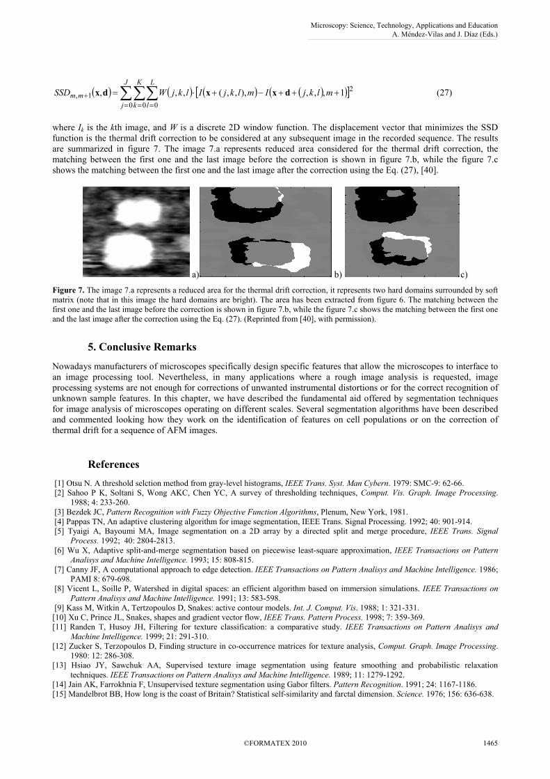
where Ik is the kth image, and W is a discrete 2D window function. The displacement vector that minimizes the SSD
function is the thermal drift correction to be considered at any subsequent image in the recorded sequence. The results
are summarized in figure 7. The image 7.a represents reduced area considered for the thermal drift correction, the
matching between the first one and the last image before the correction is shown in figure 7.b, while the figure 7.c
shows the matching between the first one and the last image after the correction using the Eq. (27), [40].
a) b) c)
Figure 7. The image 7.a represents a reduced area for the thermal drift correction, it represents two hard domains surrounded by soft
matrix (note that in this image the hard domains are bright). The area has been extracted from figure 6. The matching between the
first one and the last image before the correction is shown in figure 7.b, while the figure 7.c shows the matching between the first one
and the last image after the correction using the Eq. (27). (Reprinted from [40], with permission).
5. Conclusive Remarks
Nowadays manufacturers of microscopes specifically design specific features that allow the microscopes to interface to
an image processing tool. Nevertheless, in many applications where a rough image analysis is requested, image
processing systems are not enough for corrections of unwanted instrumental distortions or for the correct recognition of
unknown sample features. In this chapter, we have described the fundamental aid offered by segmentation techniques
for image analysis of microscopes operating on different scales. Several segmentation algorithms have been described
and commented looking how they work on the identification of features on cell populations or on the correction of
thermal drift for a sequence of AFM images.
References
[1] Otsu N. A threshold selction method from gray-level histograms, IEEE Trans. Syst. Man Cybern. 1979: SMC-9: 62-66.
[2] Sahoo P K, Soltani S, Wong AKC, Chen YC, A survey of thresholding techniques, Comput. Vis. Graph. Image Processing.
1988; 4: 233-260.
[3] Bezdek JC, Pattern Recognition with Fuzzy Objective Function Algorithms, Plenum, New York, 1981.
[4] Pappas TN, An adaptive clustering algorithm for image segmentation, IEEE Trans. Signal Processing. 1992; 40: 901-914.
[5] Tyaigi A, Bayoumi MA, Image segmentation on a 2D array by a directed split and merge procedure, IEEE Trans. Signal
Process. 1992; 40: 2804-2813.
[6] Wu X, Adaptive split-and-merge segmentation based on piecewise least-square approximation, IEEE Transactions on Pattern
Analisys and Machine Intelligence. 1993; 15: 808-815.
[7] Canny JF, A computational approach to edge detection. IEEE Transactions on Pattern Analisys and Machine Intelligence. 1986;
PAMI 8: 679-698.
[8] Vicent L, Soille P, Watershed in digital spaces: an efficient algorithm based on immersion simulations. IEEE Transactions on
Pattern Analisys and Machine Intelligence. 1991; 13: 583-598.
[9] Kass M, Witkin A, Tertzopoulos D, Snakes: active contour models. Int. J. Comput. Vis. 1988; 1: 321-331.
[10] Xu C, Prince JL, Snakes, shapes and gradient vector flow, IEEE Trans. Pattern Process. 1998; 7: 359-369.
[11] Randen T, Husoy JH, Filtering for texture classification: a comparative study. IEEE Transactions on Pattern Analisys and
Machine Intelligence. 1999; 21: 291-310.
[12] Zucker S, Terzopoulos D, Finding structure in co-occurrence matrices for texture analysis, Comput. Graph. Image Processing.
1980: 12: 286-308.
[13] Hsiao JY, Sawchuk AA, Supervised texture image segmentation using feature smoothing and probabilistic relaxation
techniques. IEEE Transactions on Pattern Analisys and Machine Intelligence. 1989; 11: 1279-1292.
[14] Jain AK, Farrokhnia F, Unsupervised texture segmentation using Gabor filters. Pattern Recognition. 1991; 24: 1167-1186.
[15] Mandelbrot BB, How long is the coast of Britain? Statistical self-similarity and farctal dimension. Science. 1976; 156: 636-638.
Microscopy: Science, Technology, Applications and Education A. Méndez-Vilas and J. Díaz (Eds.)
©FORMATEX 2010 1465
______________________________________________

[16] Pentland AP, Fractal based description of natural scenes. IEEE Transactions on Pattern Analisys and Machine Intelligence.
1984; PAMI 6: 661-674.
[17] Liu X, Tan J, Hatem I, Smith BL, Image processing of hematoxylin and eosin-stained tissues for pathological evaluation.
Toxicology Mech. Methods. 2002: 14: 301-307.
[18]Jonard S, Robert Y, Dewailly D, Revisting the ovarian volume as a diagnistic criterion for polycistic ovaries. Human
Reproduction. 2005; 20: 2893-2898.
[19] Allemand MC, Tummon IS, Phy JL, Foony SC, Dumesic DA, Sesion DR. Diagnosis of polycystic ovarioes by three –
dimensional transvaginal ultrasound. Fertility and Sterility. 2006; 85: 214-219.
[20] Danti S, D'Acunto M, Trombi L, Berrettini S, Pietrabissa A. A Micro/Nanoscale Surface Mechanical Study on Morpho-
Functional Changes in Multilineage-Differentiated Human Mesenchymal Stem Cells. Macromolecular Bioscence. 2007; 7:
589-598.
[21] Lindenbaum M, Fischer M, Bruckstein A, ON Gabor contribution to image enhancement. Pattern Recognition. 1994: 27: 1-8.
[22] Rudin L, Osher S, Fatemi E, Nonlinear total variation based noise removal algorithms. Physica D. 1992; 60: 259-268.
[23] Yaroslavsky L, Digital Picture Processing- An Introduction. Springer-Verlag, 1985.
[24] Coiffman R, Donoho D, Translation-invariant de-noising. In: Wavelets and Statistics. Springer-Verlag; 1995: 125-150.
[25] Osher S, Sole A, Vese L, Image decomposition and restoring using total variation minimization and the h-1 norm. Multiscale
Modeling and Simulation. 2003: 1(3): 349-370.
[26] Rodrigues I, Sanches J, Bioucas-Dias J. Denoising of biomedical images corrupted by Possion noise. In: Proceedings of the
International Conference on Image Processing, San Diego 2008: 1756-1759.
[27] Buades A, Coll B, Morel JM. A non-local algorithm for image denoising. In: Proceedings of the IEEE Computer Society
Conference on Computer Vision and Pattern Recognition. 2005; 2: 60-65.
[28] Mahmoudi M, Shapiro G, Fast image and video denoising via nonlocal means of similar neighborhoods. IEEE Signal
Processing Letters. 2005; 12: 839-842.
[29] Dabov K, Foi A, Katkovnik Egiazarian K, Image denoising by sparse 3D-transform domain collaborative filtering. IEEE
Transactions on Image Processing. 2007; 16: 2080-2095.
[30]Mohideen SK, Perumal AS, Sathik MM, Image denoising using discrete Wavelet Transform. International Journal Computer
Science and Network Security. 2008; 8: 213-216.
[31] Gonzalez RC, and Wood RE. Digital Image Processing. Pearson Education, 2002.
[32] Sezgin M, Sankur B. Survey over image thresholding techniques and quantitative performence evolution. J. Electron Imaging.
2004; 13: 146-165.
[33] YU J, Tan J. Objecy density-based image segmentation and its applications in biomedical image analysis. Computer methods
and Program in Biomedicine. 2009; 96: 193-204.
[34] Colantonio S, Salvetti O, Gurevich I. A two-step approach for automatic microscopic image segmentation using fuzzy clustering
and neural discrimination. Pattern recognition and Image Analysis, 2006; 17: 428-437.
[35] Yang HF, Choe Y, Cell tracking and segmentation in Electron Microscopy images using Graph Cuts. In Proceedings of the
IEEE International Symposium on Biomedical Imaging, 2009. In press.
[36] Chuklanov AP, Ziganshina SA, Bukharaev AA, Computer program for the grain analysis of AFM images of nanoparticles
placed on a rough surface. Surface and Interface Analysis. 2006; 38: 679-681.
[37] Salmons BD, Katz DR, Trawick ML, Correction of distortion due to thermal drift in scanning probe microscopy.
Ultramicroscopy, 2010; 110: 339-349.
[38] Lapshin RV, Automatic drift elimination in probe microscope images based on techniques of counter-scanning and topography
feature recognition. Measurement Science and Technology. 2007; 18: 907-927.
[39] ScheierHW, Garcia D, Sutton MA, Advances in light microscope stereo vision. Experimental Mechanics 2004; 44: 278-288.
[40] D’Acunto and Salvetti, Pattern recognition imaging for AFM measurements. In: Gurevich I, Niemann H, Salvetti O, IMT: Image
Mining Theory and Applications, , 2010: 68-77.
[41] Horn BKP, Schunck BG, Determining optical flow. Artificial Intelligence. 1981; 17: 185-204.
[42] Flore FC, de Alencar Lotufo R, Watershed from propagated markers: An interactive method to morphological object
segmentation in image sequences. Image and Vision Computing. Available on line 7 July 2009.
Microscopy: Science, Technology, Applications and Education A. Méndez-Vilas and J. Díaz (Eds.)
1466 ©FORMATEX 2010
______________________________________________