ILOG AMPL CPLEX System Version 8.0 User’s Guideliberti/teaching/xct/cplex/cplex-ampl-8.0.pdf · I...
94
© Copyright 2002 by ILOG This document and the software described in this document are the property of ILOG and are protected as ILOG trade secrets. They are furnished under a license or non-disclosure agreement, and may be used or copied only within the terms of such license or non-disclosure agreement. No part of this work may be reproduced or disseminated in any form or by any means, without the prior written permission of ILOG S.A. The AMPL Modeling System software is copyrighted by Bell Laboratories and is distributed under license by ILOG. CPLEX is a registered trademark of ILOG. Printed in France ILOG AMPL CPLEX System Version 8.0 User’s Guide Standard (Command-line) Version Including CPLEX Directives September 2002
Transcript of ILOG AMPL CPLEX System Version 8.0 User’s Guideliberti/teaching/xct/cplex/cplex-ampl-8.0.pdf · I...

© Copyright 2002 by ILOG
This document and the software described in this document are the property of ILOG and are protected as ILOG trade secrets. They are furnished under a license or non-disclosure agreement, and may be used or copied only within the terms of such license or non-disclosure agreement.
No part of this work may be reproduced or disseminated in any form or by any means, without the prior written permission of ILOG S.A.The AMPL Modeling System software is copyrighted by Bell Laboratories and is distributed under license by ILOG. CPLEX is a registered trademark of
ILOG.Printed in France
ILOG AMPL CPLEX System
Version 8.0
User’s Guide
Standard (Command-line) Version Including CPLEX Directives
September 2002


C O N T E N T S
Contents
Chapter 1 Introduction . . . . . . . . . . . . . . . . . . . . . . . . . . . . . . . . . . . . . . . . . . . . . . . . . . . . . . . 1
Welcome to AMPL . . . . . . . . . . . . . . . . . . . . . . . . . . . . . . . . . . . . . . . . . . . . . . . . . . . . . . . . . . .1
Using this guide . . . . . . . . . . . . . . . . . . . . . . . . . . . . . . . . . . . . . . . . . . . . . . . . . . . . . . . . . . . . .1
Installing AMPL . . . . . . . . . . . . . . . . . . . . . . . . . . . . . . . . . . . . . . . . . . . . . . . . . . . . . . . . . . . . .2
Chapter 2 Using AMPL. . . . . . . . . . . . . . . . . . . . . . . . . . . . . . . . . . . . . . . . . . . . . . . . . . . . . . . . 7
Running AMPL . . . . . . . . . . . . . . . . . . . . . . . . . . . . . . . . . . . . . . . . . . . . . . . . . . . . . . . . . . . . . .7
Using a text editor . . . . . . . . . . . . . . . . . . . . . . . . . . . . . . . . . . . . . . . . . . . . . . . . . . . . . . . . . . .7
Running AMPL in batch mode . . . . . . . . . . . . . . . . . . . . . . . . . . . . . . . . . . . . . . . . . . . . . . . . .8
Chapter 3 AMPL-Solver Interaction . . . . . . . . . . . . . . . . . . . . . . . . . . . . . . . . . . . . . . . . . . . . 11
Choosing a solver . . . . . . . . . . . . . . . . . . . . . . . . . . . . . . . . . . . . . . . . . . . . . . . . . . . . . . . . . .11
Specifying solver options . . . . . . . . . . . . . . . . . . . . . . . . . . . . . . . . . . . . . . . . . . . . . . . . . . . .12
Initial variable values and solvers . . . . . . . . . . . . . . . . . . . . . . . . . . . . . . . . . . . . . . . . . . . . .13
Problem and solution files . . . . . . . . . . . . . . . . . . . . . . . . . . . . . . . . . . . . . . . . . . . . . . . . . . .13
Running solvers outside AMPL . . . . . . . . . . . . . . . . . . . . . . . . . . . . . . . . . . . . . . . . . . . . . . .16
Using MPS file format . . . . . . . . . . . . . . . . . . . . . . . . . . . . . . . . . . . . . . . . . . . . . . . . . . . . . . .16
Temporary files directory . . . . . . . . . . . . . . . . . . . . . . . . . . . . . . . . . . . . . . . . . . . . . . . . . . . .17
Chapter 4 Customizing AMPL . . . . . . . . . . . . . . . . . . . . . . . . . . . . . . . . . . . . . . . . . . . . . . . . 19
Command line switches . . . . . . . . . . . . . . . . . . . . . . . . . . . . . . . . . . . . . . . . . . . . . . . . . . . . .19
Persistent option settings . . . . . . . . . . . . . . . . . . . . . . . . . . . . . . . . . . . . . . . . . . . . . . . . . . . .20
I L O G A M P L C P L E X S Y S T E M 8 . 0 — U S E R ’ S G U I D E v

T A B L E O F C O N T E N T S
Chapter 5 Using CPLEX with AMPL . . . . . . . . . . . . . . . . . . . . . . . . . . . . . . . . . . . . . . . . . . . . 23
Problems handled by CPLEX . . . . . . . . . . . . . . . . . . . . . . . . . . . . . . . . . . . . . . . . . . . . . . . . .23
Specifying CPLEX directives . . . . . . . . . . . . . . . . . . . . . . . . . . . . . . . . . . . . . . . . . . . . . . . . .25
Chapter 6 Using CPLEX for Linear Programming. . . . . . . . . . . . . . . . . . . . . . . . . . . . . . . . . 29
CPLEX linear programming algorithms. . . . . . . . . . . . . . . . . . . . . . . . . . . . . . . . . . . . . . . . .29
Directives for problem and algorithm selection . . . . . . . . . . . . . . . . . . . . . . . . . . . . . . . . . .30
Directives for preprocessing . . . . . . . . . . . . . . . . . . . . . . . . . . . . . . . . . . . . . . . . . . . . . . . . .32
Directives for controlling the simplex algorithm . . . . . . . . . . . . . . . . . . . . . . . . . . . . . . . . .34
Directives for controlling the barrier algorithm . . . . . . . . . . . . . . . . . . . . . . . . . . . . . . . . . .38
Directives for improving stability . . . . . . . . . . . . . . . . . . . . . . . . . . . . . . . . . . . . . . . . . . . . . .40
Directives for starting and stopping . . . . . . . . . . . . . . . . . . . . . . . . . . . . . . . . . . . . . . . . . . .41
Directives for controlling output . . . . . . . . . . . . . . . . . . . . . . . . . . . . . . . . . . . . . . . . . . . . . .43
Chapter 7 Using CPLEX for Integer Programming . . . . . . . . . . . . . . . . . . . . . . . . . . . . . . . . 45
CPLEX mixed integer algorithm . . . . . . . . . . . . . . . . . . . . . . . . . . . . . . . . . . . . . . . . . . . . . . .45
Directives for preprocessing . . . . . . . . . . . . . . . . . . . . . . . . . . . . . . . . . . . . . . . . . . . . . . . . .47
Directives for algorithmic control. . . . . . . . . . . . . . . . . . . . . . . . . . . . . . . . . . . . . . . . . . . . . .50
Directives for relaxing optimality . . . . . . . . . . . . . . . . . . . . . . . . . . . . . . . . . . . . . . . . . . . . . .56
Directives for halting and resuming the search . . . . . . . . . . . . . . . . . . . . . . . . . . . . . . . . . .57
Directives for controlling output . . . . . . . . . . . . . . . . . . . . . . . . . . . . . . . . . . . . . . . . . . . . . .60
Common difficulties. . . . . . . . . . . . . . . . . . . . . . . . . . . . . . . . . . . . . . . . . . . . . . . . . . . . . . . . .60
Chapter 8 Defined Suffixes for CPLEX. . . . . . . . . . . . . . . . . . . . . . . . . . . . . . . . . . . . . . . . . . 65
Algorithmic control . . . . . . . . . . . . . . . . . . . . . . . . . . . . . . . . . . . . . . . . . . . . . . . . . . . . . . . . .65
Sensitivity ranging. . . . . . . . . . . . . . . . . . . . . . . . . . . . . . . . . . . . . . . . . . . . . . . . . . . . . . . . . .67
Diagnosing infeasibilities . . . . . . . . . . . . . . . . . . . . . . . . . . . . . . . . . . . . . . . . . . . . . . . . . . . .68
Direction of unboundedness . . . . . . . . . . . . . . . . . . . . . . . . . . . . . . . . . . . . . . . . . . . . . . . . .70
Chapter 9 CPLEX status codes in AMPL . . . . . . . . . . . . . . . . . . . . . . . . . . . . . . . . . . . . . . . . 73
Solve codes . . . . . . . . . . . . . . . . . . . . . . . . . . . . . . . . . . . . . . . . . . . . . . . . . . . . . . . . . . . . . . .73
Basis status . . . . . . . . . . . . . . . . . . . . . . . . . . . . . . . . . . . . . . . . . . . . . . . . . . . . . . . . . . . . . . .76
Index . . . . . . . . . . . . . . . . . . . . . . . . . . . . . . . . . . . . . . . . . . . . . . . . . . . . . . . . . . . . . . . . . . . . . . . . . 81
vi I L O G A M P L C P L E X S Y S T E M 8 . 0 — U S E R ’ S G U I D E

C H A P T E R
Intro
du
ction
1
Introduction
Welcome to AMPL
Welcome to the AMPL Modeling System—a comprehensive, powerful, algebraic modeling language for problems in linear, nonlinear, and integer programming. AMPL is based upon modern modeling principles and utilizes an advanced architecture providing flexibility most other modeling systems lack. AMPL has been proven in commercial applications, and is successfully used in demanding model applications around the world.
AMPL helps you create models with maximum productivity. By using AMPL's natural algebraic notation, even a very large, complex model can often be stated in a concise (often less than one page), understandable form. As its models are easy to understand, debug, and modify, AMPL also makes maintaining models easy.
Using this guide
This brief guide describes starting up AMPL, reading a model and supplying data, and solving (optimizing) the model using CPLEX. The first three sections cover issues such as using command-line options and environment variables and using AMPL on different operating systems. Later sections provide a detailed description of CPLEX directives.
I L O G A M P L C P L E X S Y S T E M 8 . 0 — U S E R ’ S G U I D E 1

I N S T A L L I N G A M P L
This document does not provide full installation and set-up instructions. Documentation describing other AMPL-compatible solvers distributed by ILOG is also available separately.
This Guide does not teach you the AMPL language. To learn and effectively use the features of the AMPL language, you should have a copy of the book AMPL: A Modeling Language for Mathematical Programming by Robert Fourer, David M. Gay and Brian W. Kernighan (ISBN 0-534-50983-5, first published in 1993 by The Scientific Press, now published by Duxbury Press). This book includes a tutorial on AMPL and optimization modeling; models for many "classical" problems such as production, transportation, blending, and scheduling; discussions of modeling concepts such as linear, nonlinear and piecewise-linear models, integer linear models, and columnwise formulations; and a reference section.
AMPL is continuously undergoing development, and while we strive to keep users updated on language features and capabilities, the official reference to the language is the AMPL book, which is naturally revised less frequently.
Installing AMPL
Please read these instructions in their entirety before beginning the installation. Remember that most distributions will operate properly only on the specific platform and operating system version for which they were intended. If you upgrade your operating system you may need to obtain a new distribution.
All AMPL installations include cplexamp (cplexamp.exe on Windows), the CPLEX solver for AMPL. This combined distribution is known as the AMPL/CPLEX system.
Note that cplexamp may not be licensed for a few users with unsupported solvers. However, most AMPL installations will include the use of cplexamp.
Requirements
AMPL may be installed and run on the following configurations:
Table 1.1 AMPL configuration table
Computer Operating System Release
DEC Alpha DEC UNIX 4.0 and higher
HP PA-7xxx HP-UX 11 and higher
HP PA-8xxx HP-UX 11 and higher
Intel PC Linux 2.1 and higher
Intel PC Windows NT 3.5 and higher
2 I L O G A M P L C P L E X S Y S T E M 8 . 0 — U S E R ’ S G U I D E

I N S T A L L I N G A M P L
Intro
du
ction
Unix installation
On Unix systems, AMPL is installed into the current working directory. We recommend that you perform the installation in an empty directory. After installation, make sure the executable files have read and execute privileges turned on for all users and accounts that will use AMPL.
CD-ROM
The ILOG CD contains the AMPL/CPLEX system for several different platforms. First, read the file INFO_UNX.TXT. The section titled, "AMPL Modeling Language" contains information to help you locate the distribution for your platform. Note that the files listed in this section contain the entire AMPL/CPLEX System, not just the AMPL language processor. After you have located the files, read the CD booklet for instructions on extracting the distribution.
FTP
Execute:
gzip-dc < /path/ampl.tgz | tar xf -
where /path is the full path name into which ampl.tgz was downloaded.
AMPL and Parallel CPLEX (except for Linux)
If you have purchased AMPL and Parallel CPLEX, follow the above instructions for the appropriate media. Then rename cplexamp to cplexamp.ser and rename parcplexamp to cplexamp.
Windows installation
On Windows systems AMPL is installed into a directory which you can specify during the installation (the default location is C:\AMPL).
Intel PC Windows 9x/2000
RS6000 or PowerPC AIX 4.3 and higher
SGI 32-bit (MIPS3) Irix 6.5 and higher
SGI 64-bit (MIPS4) Irix 6.5 and higher
Sun SPARC Solaris 2.6 and higher
Sun Ultra Solaris 2.6 and higher
Table 1.1 AMPL configuration table (Continued)
Computer Operating System Release
I L O G A M P L C P L E X S Y S T E M 8 . 0 — U S E R ’ S G U I D E 3

I N S T A L L I N G A M P L
CD-ROM
The ILOG CD contains the AMPL/CPLEX system for several different platforms. First, read the file INFO_PC.TXT. The section titled, "AMPL Modeling Language" contains information to help you locate the distribution for your version of Windows. Note that the files listed in this section contain the entire AMPL/CPLEX System, not just the AMPL language processor. After you have located the files, read the CD booklet for instructions on setting up the distribution.
FTP
After downloading the files, execute SETUP.EXE from the Run dialog or in an MS-DOS window. Follow the instructions presented by the setup program. To access the Run dialog box on Windows, click on the Start button and select Run…
AMPL and Parallel CPLEX
If you have purchased the AMPL and Parallel CPLEX, follow the above installation instructions for the appropriate media. The AMPL/CPLEX System will automatically use the parallel processors available on your computer provided your license configuration includes the parallel option.
Licensing
AMPL is licensed in the same way as CPLEX. If you have already activated a license for the CPLEX Suite on this machine and you are not adding AMPL as a new feature, then AMPL is already licensed, and you should skip these licensing instructions.
Updating an existing license
If you are upgrading from a previous version of CPLEX, please refer to the CPLEX License Update Instructions (provided separately) or contact the CPLEX License Administrator. You should skip any installation steps that would establish a new license.
New installation
If you are installing CPLEX or AMPL for the first time, you will receive an ILOG License Manager (ILM) manual and a license key that enables the use of AMPL and/or CPLEX. Follow the instructions in that manual for details on how to install the license key.
Usage notes
The CPLEX solver for AMPL is named cplexamp (cplexamp.exe on Windows). This version of AMPL will use this solver by default. Older versions of the CPLEX solver for AMPL were simply named cplex (cplex.exe on Windows). Some users of that version may have specified the solver in their model or run files like this:
option solver cplex;
4 I L O G A M P L C P L E X S Y S T E M 8 . 0 — U S E R ’ S G U I D E

I N S T A L L I N G A M P L
Intro
du
ction
If you have models containing settings like this, you will encounter errors (or the old version of the solver might be invoked). There are two ways to fix this. Ideally, you should change these lines to:
If that is not practical, you can copy the file cplexamp to cplex. If you do the latter, you must remember to copy it again the next time you upgrade cplexamp.
Parallel users of the barrier method on the Sun UltraSparc will need to set the PARALLEL system environment variable to a value greater than or equal to the number of licensed threads. For example, from the C shell the command
will enable the parallel CPLEX solver for AMPL to use 4 threads, subject to license restrictions.
option solver cplexamp;
setenv PARALLEL 4
I L O G A M P L C P L E X S Y S T E M 8 . 0 — U S E R ’ S G U I D E 5

I N S T A L L I N G A M P L
Installed files
Unix systems
Windows systems
Examples
Parallel systems
On systems that support parallelization, additional files may be present:
Unix
ampl AMPL
cplexamp The CPLEX solver for AMPL
examples.txt Description of the example files (installed with the examples)
ampl.exe AMPL
cplexamp.exe The CPLEX solver for AMPL
uninst.isu File used by the Windows uninstall procedure
ampltabl.dll ODBC database interface
/models Sample AMPL models - Most of these correspond to examples in the AMPL book. More information on some of the examples is provided in the readme file in this directory.
/looping Advanced sample AMPL models - A description of each is provided in the readme file in this directory.
/compass/finance/compass/invest/compass/logistic/compass/product/compass/purchase/compass/schedule
More samples - The compass directory is sub-divided into industry-specific subdirectories. The models have been brought together from a variety of sources. Together, they provide a palette of AMPL models that you may use as a starting point for your projects.
parcplexamp Parallel CPLEX solver for AMPL
6 I L O G A M P L C P L E X S Y S T E M 8 . 0 — U S E R ’ S G U I D E

C H A P T E R
Usin
g A
MP
L
2
Using AMPL
Running AMPL
If you have added the AMPL installation directory to the search path, you can run AMPL from any directory. Otherwise, run AMPL by moving to the AMPL directory and typing ampl at the shell prompt.
At the ampl: prompt, you can type any AMPL language statement, or any of the commands described in Section A.13 of the book AMPL: A Modeling Language for Mathematical Programming. To end the session, type quit; at the ampl: prompt.
Using a text editor
Generally, you will edit your model and data (both expressed using AMPL language statements) in a text editor, and type commands at the ampl: prompt to load your model and data, solve a problem, and inspect the results. Although you could type in the statements of a model at the ampl: prompt, AMPL does not include a built-in text editor, so you cannot use AMPL commands to edit the statements you have previously entered. Microsoft Windows users (on PCs) and XWindows users (on Unix systems) should open separate windows for editing files and running AMPL.
I L O G A M P L C P L E X S Y S T E M 8 . 0 — U S E R ’ S G U I D E 7

R U N N I N G A M P L I N B A T C H M O D E
If you cannot open multiple windows on your desktop, you can use AMPL’s shell command to invoke an editor from within AMPL. You can use any editor that saves files in ASCII format. Windows command-line (DOS) users can use edit or notepad and Unix users vi or emacs. If you are using edit under DOS, for instance, you can type:
Use editor menus and commands to edit your file, then save it and exit the editor. At the ampl: prompt you can type new AMPL commands, such as:
Note that editing a file in a text editor does not affect your AMPL session until you explicitly reload the edited file, as shown above.
Running AMPL in batch mode
If you have previously developed a model and its data, and would like to solve it and display the results automatically, you can create a file containing the commands you would like AMPL to execute, and specify that file at the command line when you run AMPL. For example, you might create a file called steel.run, containing the commands:
Note that this assumes that steel.run is in the same directory as the model and data files, and that AMPL can be found on the path.
You can then run AMPL as follows:
A more flexible approach, which is a commonly followed convention among AMPL users, is to put just the AMPL commands (the last three lines in the example above) in a file with the *.run extension. You can then type:
which accomplishes the same thing as:
ampl: shell ’edit steel.dat’;
ampl: reset data;ampl: data steel.dat;
model steel.mod;data steel.dat;option solver cplexamp;solve;display Make >steel.ans;
C:\> ampl steel.run
C:\> ampl steel.mod steel.dat steel.run
C:\> amplampl: include steel.mod;ampl: include steel.dat;ampl: include steel.run;ampl: quit;C:\>
8 I L O G A M P L C P L E X S Y S T E M 8 . 0 — U S E R ’ S G U I D E

Usin
g A
MP
L
R U N N I N G A M P L I N B A T C H M O D E
If you intend to load several files and solve a problem, but you want to type a few interactive commands in the middle of the process, type the character – in place of a filename. AMPL processes the files on the command line from left to right; when it encounters the – symbol it displays the ampl: prompt and accepts commands until you type end;. For example, you could type:
This will solve the problem as before, but with the parameter avail set to 50 instead of 40 (the value specified in steel.dat). To start AMPL, load a model and data file, and wait for your interactive commands, type:
C:\> ampl steel.mod steel.dat - steel.runampl: let avail := 50;ampl: end;
C:\> ampl steel.mod steel.dat -
I L O G A M P L C P L E X S Y S T E M 8 . 0 — U S E R ’ S G U I D E 9

R U N N I N G A M P L I N B A T C H M O D E
10 I L O G A M P L C P L E X S Y S T E M 8 . 0 — U S E R ’ S G U I D E

C H A P T E R
AM
PL
-So
lver In
teraction
3
AMPL-Solver Interaction
Choosing a solver
AMPL’s solver interface supports linear, nonlinear, and mixed integer models with no built-in size limitations. This interface is rich enough to support many of the features used by advanced solvers to improve performance and solution accuracy, such as piecewise-linear constructs, representation of network problems, and automatic differentiation of nonlinear functions. To take advantage of these features, solvers must be written to utilize AMPL’s interface. ILOG provides no support for the usage of AMPL with solvers not distributed by ILOG.
You choose a solver for a particular problem by giving its executable filename in the AMPL option solver command. For example, to use the (AMPL-compatible) CPLEX solver, type:
Most solvers have algorithmic options, such as CPLEX with its Mixed Integer and Barrier options. In these cases, you give the solver executable name to AMPL (for example, with option solver cplexamp); the solver will determine, from the problem characteristics as passed by AMPL (for example, a quadratic objective or integer variables) as well as solver options you specify, which algorithmic options will be used.
ampl: option solver cplexamp;
I L O G A M P L C P L E X S Y S T E M 8 . 0 — U S E R ’ S G U I D E 11

S P E C I F Y I N G S O L V E R O P T I O N S
Specifying solver options
You can specify option settings for a particular solver through the AMPL option command. (CPLEX-specific directives are described later in this document.) Since all solvers provide default settings for their options, this is necessary only when your problem requires certain nondefault settings in order to solve, or when certain settings yield improved performance or solution accuracy.
To specify solver options, enter
where solver is replaced by the name of the solver you are using. This approach allows you to set up different options for each solver you use and to switch among them by simply choosing the appropriate solver with the option solver command. For example:
Solver options consist of an identifier alone, or an identifier followed by an = sign and a value. Some solvers treat uppercase and lowercase versions of an option identifier as equivalent, while others are sensitive to case, so that RELAX is not the same as relax, for example.
Solver option settings can easily become long enough to stretch over more than one line. In such cases you can either continue a single quoted string by placing a \ character at the end of each line, as in:
Or you can write a series of individually quoted strings, which will be concatenated automatically by AMPL, as in:
If you use the latter approach, be sure to include spaces at the beginning or end of the individual strings, so that the identifiers will be separated by spaces when all of the strings are concatenated.
Often you will want to add solver options to the set you are currently using. If you simply type a command such as option solver_options ’new options’; however, you will overwrite the existing option settings. To avoid this problem, you can use AMPL’s $ notation for options: the symbol $option_name is replaced by the current value of
option solver_options ’settings’;
ampl: option cplex_options ’relax scale=1’;
ampl: option cplex_options ’crash=0 dual \ampl? feasibility=1.0e-8 scale=1 \ampl? lpiterlim=100’;
ampl: option cplex_options ’crash=0 dual’ampl? ’ feasibility=1.0e-8 scale=1’ampl? ’ lpiterlim=100’;
12 I L O G A M P L C P L E X S Y S T E M 8 . 0 — U S E R ’ S G U I D E
AM
PL
-So
lver In
teraction
I N I T I A L V A R I A B L E V A L U E S A N D S O L V E R S
option_name. To add an optimality tolerance to the CPLEX options in the above example, you would write:
Initial variable values and solvers
Some optimizers (including most nonlinear solvers but excluding simplex-based linear solvers) make use of initial values for the decision variables as a starting point in their search for an optimal solution. A good choice of initial values can greatly speed up the solution process in some cases. Moreover, in nonlinear models with multiple local optima, the optimal solution reported by the solver may depend on the initial values for the variables.
AMPL passes initial values for decision variables, and dual values if available, to the solver. You can set initial values using the := syntax in the var declaration of your AMPL model.
When you solve a problem two times in a row, the final values from the first solver invocation become the initial values for the second solver invocation (unless you override this behavior with statements in your AMPL model). In nonlinear models with multiple local optima, this can cause some solvers to report a different solution on the second invocation.
Simplex-based solvers typically discard initial values. However, they can use basis status information, if available. Basis statuses can be set either within AMPL or by a previous optimization. Information on interpreting and setting variable statuses is provided in Chapter 9, CPLEX status codes in AMPL.
Problem and solution files
When you type solve; AMPL processes your model and data to create a temporary problem file, such as steel.nl, which will be read by the solver. It then loads and executes the solver program, which is responsible for creating a solution file such as steel.sol. AMPL reads the solution file and makes the solution values available through the variable, constraint, and objective names you have declared in your AMPL model. Unless you specify otherwise, AMPL then deletes the temporary problem and solution files.
You can display the solution information, for example the values of the decision variables and constraints, in your AMPL session with commands such as display. For example, if you have just solved a problem created from steel.mod and steel.dat, you could type:
ampl: option cplex_options $cplex_optionsampl? ’ optimality=1.0e-8’;
ampl: display Make, Time;
I L O G A M P L C P L E X S Y S T E M 8 . 0 — U S E R ’ S G U I D E 13

P R O B L E M A N D S O L U T I O N F I L E S
To save this output in a file, you can use redirection:
Note that when you simply mention the name of a constraint in a display statement, AMPL will display the dual value (shadow price) of that constraint, not its left-hand side value. You can use the AMPL suffix notation to display the left-hand side value, as described in the book AMPL: A Modeling Language for Mathematical Programming.
Saving temporary files
AMPL deletes the temporary problem (*.nl) and solution (*.sol) files after a solver is finished, so no permanent record of the solution is kept unless you save the output yourself (for example, using display with redirection as illustrated above). To override the deletion of temporary files, you can use the AMPL write command. For example:
The first letter, b, in the filename portion of the write command is interpreted specially, as explained below. If you now display the files in the current directory with a command such as dir steel.*, you will find the problem file steel.nl and the solution file steel.sol.
To later view the solution values, you would use the solution command. For example:
You must include the model and data statements, as shown above, so that AMPL knows the definitions of symbolic names like Make. But solution then retrieves the earlier results from steel.sol, without running a solver.
if you use b as the first character of the filename portion of the write command, AMPL uses a compact and efficient binary format for the problem and solution files. If you use g instead, AMPL writes the files in an ASCII format that may be easier to transmit electronically over systems like the Internet. In technical support and consulting situations,
ampl: display Make, Time > mysol.txt;
C:\> amplampl: model steel.mod; data steel.dat;ampl: write bsteel;ampl: solve;CPLEX 8.0: optimal solution; objective 1920002 iterations (0 in phase I)ampl: quit;
C:\> amplampl: model steel.mod; data steel.dat;ampl: solution steel.sol;CPLEX 8.0: optimal solution; objective 1920002 iterations (0 in phase I)ampl: display Make;Make [*] :=bands 6000coils 1400;ampl: quit;
14 I L O G A M P L C P L E X S Y S T E M 8 . 0 — U S E R ’ S G U I D E
AM
PL
-So
lver In
teraction
P R O B L E M A N D S O L U T I O N F I L E S
ILOG may ask you to send a file using this format. If you use m, AMPL writes the problem in MPS format, and the filename ends in mps (for example, steel.mps). This is described further in Using MPS file format on page 16.
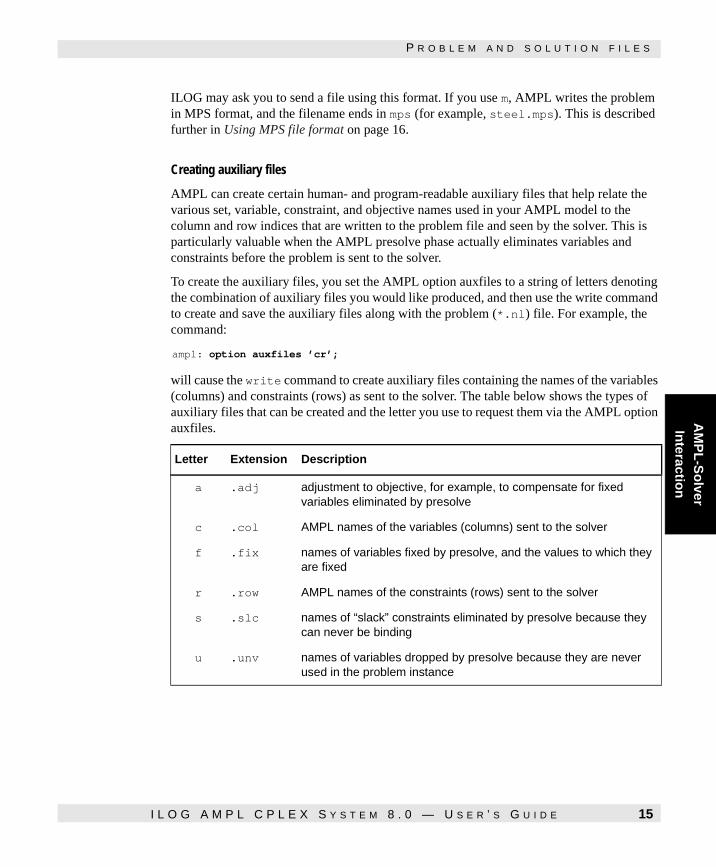
Creating auxiliary files
AMPL can create certain human- and program-readable auxiliary files that help relate the various set, variable, constraint, and objective names used in your AMPL model to the column and row indices that are written to the problem file and seen by the solver. This is particularly valuable when the AMPL presolve phase actually eliminates variables and constraints before the problem is sent to the solver.
To create the auxiliary files, you set the AMPL option auxfiles to a string of letters denoting the combination of auxiliary files you would like produced, and then use the write command to create and save the auxiliary files along with the problem (*.nl) file. For example, the command:
will cause the write command to create auxiliary files containing the names of the variables (columns) and constraints (rows) as sent to the solver. The table below shows the types of auxiliary files that can be created and the letter you use to request them via the AMPL option auxfiles.
ampl: option auxfiles ’cr’;
Letter Extension Description
a .adj adjustment to objective, for example, to compensate for fixed variables eliminated by presolve
c .col AMPL names of the variables (columns) sent to the solver
f .fix names of variables fixed by presolve, and the values to which they are fixed
r .row AMPL names of the constraints (rows) sent to the solver
s .slc names of “slack” constraints eliminated by presolve because they can never be binding
u .unv names of variables dropped by presolve because they are never used in the problem instance
I L O G A M P L C P L E X S Y S T E M 8 . 0 — U S E R ’ S G U I D E 15

R U N N I N G S O L V E R S O U T S I D E A M P L
Running solvers outside AMPL
With the write and solution commands, you can arrange to execute your solver outside the AMPL session. You might want to do this if you receive an out of memory message from your solver (not from AMPL itself): When the solver is invoked from within AMPL, a fair amount of memory is already used for the AMPL Modeling System program code and for data structures created by AMPL for its own use in memory. If you execute the solver alone, it can use all available memory.
To run your solver separately, first use AMPL to create a problem file:
Then run your solver with a command like the one below (for CPLEX):
In this example, the first argument steel matches the filename (after the initial letter b) in the AMPL write command. The -AMPL argument tells the solver that it is receiving a problem from AMPL. This may optionally be followed by any solver options you need for the problem, using the same syntax used with the option solver_options command but omitting the outer quotes, for example crash=1 relax. Assuming that the solver runs successfully to completion, it will write a solution file; steel.sol in this case. You can then restart AMPL and read in the results with the solution command, as outlined earlier:
Using MPS file format
MPS file format, originally developed decades ago for IBM’s Mathematical Programming System, is a widely recognized format for linear and integer programming problems. Although it is a standard supported by many solvers and modeling systems (including AMPL), MPS file format is neither compact nor easy to read and understand; AMPL’s binary file format is a much more efficient way for modeling systems and solvers to communicate. Also, MPS file format cannot be used for nonlinear problems, and not all MPS-compatible solvers support exactly the same format, particularly for mixed integer problems.
AMPL does have the ability to translate a model into MPS file format, as outlined below. With this feature, you may be able to solve AMPL models with a solver that reads its problem input in MPS file format. If you choose to use this feature, you will find AMPL’s
C:\> amplampl: model steel.mod; data steel.dat;ampl: write bsteel;ampl: quit;
C:\> cplexamp steel -AMPL solver_options
C:\> amplampl: model steel.mod; data steel.dat;ampl: solution steel.sol;
16 I L O G A M P L C P L E X S Y S T E M 8 . 0 — U S E R ’ S G U I D E

AM
PL
-So
lver In
teraction
T E M P O R A R Y F I L E S D I R E C T O R Y
ability to produce auxiliary files very useful, since these files can be used to relate the MPS file format information to the sets, variables, constraints, and objectives defined in the AMPL model. However, you will not be able to bring the solution—variable values, dual values, and so on—back into AMPL; further work with the solution must be performed outside of AMPL.
To translate your model into MPS file format, use the write command as outlined above with m as the first letter of the filename. To illustrate, the command shown below creates a file named steel.mps:
In most cases, you will need to run your solver separately to obtain the solution.
Note that the MPS format does not provide a way to distinguish between objective maximization and minimization. However, CPLEX assumes that the objective is to be minimized. (There is no standardization on this issue; other solvers may assume maximization.) Thus, it is incumbent upon the user of the MPS format to ensure that the objective sense in the AMPL model corresponds to the solver's interpretation.
Temporary files directory
If the TMPDIR option is not set, AMPL writes the problem and solution files and other temporary files to the current directory. You can give a specific location for the temporary files by setting option TMPDIR to a valid path. On a PC, you might use:
On a Unix machine, a typical choice would be:
ampl: write msteel;
ampl: option TMPDIR ’D:\temp’;
ampl: option TMPDIR ’/tmp’;
I L O G A M P L C P L E X S Y S T E M 8 . 0 — U S E R ’ S G U I D E 17

T E M P O R A R Y F I L E S D I R E C T O R Y
18 I L O G A M P L C P L E X S Y S T E M 8 . 0 — U S E R ’ S G U I D E
C H A P T E R
Cu
stom
izing
AM
PL
4
Customizing AMPL
Command line switches
Certain AMPL options normally set with the option command during an AMPL session can also be set when AMPL is first invoked. This is done using a command line switch consisting of a hyphen and a single letter, followed in some cases by a numeric or string value. You will find these switches most useful when you have one or more model, data, or run file that you want AMPL to process using different option settings at different times, without actually editing the files themselves.
The table below summarizes the command line switches and their equivalent names when set with the AMPL option command:
Switch AMPL Option Description
-Cn Cautions n n = 0: suppress caution messagesn = 1: report caution messages (default)n = 2: treat cautions as errors
-en eexit n n > 0: abandon command after n errorsn < 0: abort AMPL after |n| errorsn = 0: report any number of errors
I L O G A M P L C P L E X S Y S T E M 8 . 0 — U S E R ’ S G U I D E 19

P E R S I S T E N T O P T I O N S E T T I N G S
If you type ampl -? at the shell prompt, AMPL will display a summary list of all the command line switches. On some Unix shells, ? is a special character, so you may need to use "-?" with double quotation marks.
Persistent option settings
If you have many option settings or other commands that you would like performed each time AMPL starts, you may create a text file containing these commands (in AMPL language syntax). Then set the environment variable name OPTIONS_IN to the pathname of this text file. For example, on a Windows PC, you should type:
If you are using a C shell on a Unix machine you would type something like:
AMPL reads the file referred to by OPTIONS_IN and executes any commands therein before it reads any other files mentioned on the command line or prompts for any interactive commands.
-f funcwarn 1 do not treat unavailable functions of constant arguments as variable
-P presolve 0 turn off AMPL’s presolve phase
-S substout 1 use “defining” equations to eliminate variables
-L linelim 1 fully eliminate variables with linear “defining” equations, so model is recognized as linear
-T gentimes 1 show time to generate each model component
-t times 1 show time taken in each model translation phase
-ostr outopt str set problem file format (b, g, m) and stub name;to display more possibilities use -o?
-s randseed ‘’ use current time for random number seed
-sn randseed n use n for random number seed
-v version display the AMPL software version number
C:\> set OPTIONS_IN=c:\amplinit.txt
% setenv OPTIONS_IN ~ijr/amplinit.txt
Switch AMPL Option Description
20 I L O G A M P L C P L E X S Y S T E M 8 . 0 — U S E R ’ S G U I D E

Cu
stom
izing
AM
PL
P E R S I S T E N T O P T I O N S E T T I N G S
If you want AMPL to preserve all of your option settings from one session to the next, you can cause AMPL to write the options into a text file named by setting the AMPL option OPTIONS_INOUT:
Before exiting, AMPL writes a series of option commands to the file named by OPTIONS_INOUT which, when read, will set all of the options to the values they had at the end of the session. To use this text file, set the corresponding environment variable to the same filename:
After you do this, AMPL will read and execute the commands in amplopt.txt when it starts up. When you end a session, AMPL will write the current option settings - including any changes you have made during the session - into this file, so that they will be preserved for use in your next session.
If both the OPTIONS_IN and OPTIONS_INOUT environment variables are defined, the file referred to by OPTIONS_IN will be processed first, then the file referred to by OPTIONS_INOUT.
ampl: option OPTIONS_INOUT ’c:\amplopt.txt’;
C:\> set OPTIONS_INOUT=c:\amplopt.txt
I L O G A M P L C P L E X S Y S T E M 8 . 0 — U S E R ’ S G U I D E 21

P E R S I S T E N T O P T I O N S E T T I N G S
22 I L O G A M P L C P L E X S Y S T E M 8 . 0 — U S E R ’ S G U I D E

C H A P T E R
Usin
g C
PL
EX
with
A
MP
L
5
Using CPLEX with AMPL
Problems handled by CPLEX
CPLEX is designed to solve linear programs as described in Chapters 1-8 and 11-12 of AMPL: A Modeling Language for Mathematical Programming, as well as the integer programs described in Chapter 15. Integer programs may be pure (all integer variables) or mixed (some integer and some continuous variables); integer variables may be binary (taking values 0 and 1 only) or may have more general lower and upper bounds.
For the network linear programs described in Chapter 12, CPLEX also incorporates an especially fast network optimization algorithm.
The barrier algorithmic option to CPLEX, though originally designed to handle linear programs, also allows the solution of a special class of nonlinear problems, namely, quadratic programs (QPs), as described later in this section. However, CPLEX does not solve general (non-QP) nonlinear programs. For instance, if you attempt to solve the following nonlinear problem described in Chapter 13 of the AMPL book, CPLEX will generate an error message:
ampl: model models\nltransd.mod;ampl: data models\nltrans.dat; ampl: option solver cplexamp; ampl: solve; at0.nl contains a nonlinear objective.
ampl:
I L O G A M P L C P L E X S Y S T E M 8 . 0 — U S E R ’ S G U I D E 23
P R O B L E M S H A N D L E D B Y C P L E X
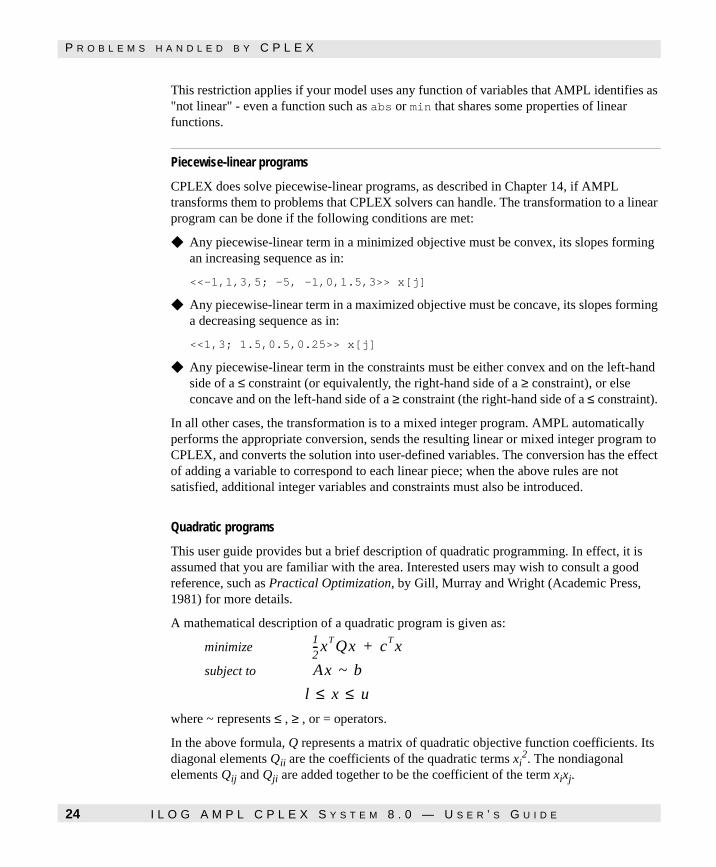
This restriction applies if your model uses any function of variables that AMPL identifies as "not linear" - even a function such as abs or min that shares some properties of linear functions.
Piecewise-linear programs
CPLEX does solve piecewise-linear programs, as described in Chapter 14, if AMPL transforms them to problems that CPLEX solvers can handle. The transformation to a linear program can be done if the following conditions are met:
◆ Any piecewise-linear term in a minimized objective must be convex, its slopes forming an increasing sequence as in:
<<-1,1,3,5; -5, -1,0,1.5,3>> x[j]
◆ Any piecewise-linear term in a maximized objective must be concave, its slopes forming a decreasing sequence as in:
<<1,3; 1.5,0.5,0.25>> x[j]
◆ Any piecewise-linear term in the constraints must be either convex and on the left-hand side of a ≤ constraint (or equivalently, the right-hand side of a ≥ constraint), or else concave and on the left-hand side of a ≥ constraint (the right-hand side of a ≤ constraint).
In all other cases, the transformation is to a mixed integer program. AMPL automatically performs the appropriate conversion, sends the resulting linear or mixed integer program to CPLEX, and converts the solution into user-defined variables. The conversion has the effect of adding a variable to correspond to each linear piece; when the above rules are not satisfied, additional integer variables and constraints must also be introduced.
Quadratic programs
This user guide provides but a brief description of quadratic programming. In effect, it is assumed that you are familiar with the area. Interested users may wish to consult a good reference, such as Practical Optimization, by Gill, Murray and Wright (Academic Press, 1981) for more details.
A mathematical description of a quadratic program is given as:
minimize
subject to
where ~ represents ≤ , ≥ , or = operators.
In the above formula, Q represents a matrix of quadratic objective function coefficients. Its diagonal elements Qii are the coefficients of the quadratic terms xi
2. The nondiagonal elements Qij and Qji are added together to be the coefficient of the term xixj.
12-- xT Qx cT x+
Ax b~
l x u≤ ≤
24 I L O G A M P L C P L E X S Y S T E M 8 . 0 — U S E R ’ S G U I D E

Usin
g C
PL
EX
with
A
MP
LS P E C I F Y I N G C P L E X D I R E C T I V E S
The CPLEX linear programming algorithms incorporate an extension for quadratic programming. For a problem to be solvable using this option, the following conditions must hold:
1. All constraints must be linear.
2. The objective must be a sum of terms, each of which is either a linear expression or a product of two linear expressions.
3. For any values of the variables (whether or not they satisfy the constraints), the quadratic part of the objective must have a nonnegative value (if a minimization) or a nonpositive value (if a maximization).
The last condition is known as positive semi-definiteness (for minimization) or negative semi-definiteness (for maximization). CPLEX automatically recognizes nonlinear problems that satisfy these conditions, and invokes the barrier algorithm to solve them. Nonlinear problems of any other kind are rejected with an appropriate message.
Most CPLEX features applying to continuous LP models apply also to continuous QP models; likewise most features applying to linear MIP models also apply to mixed-integer QP models (MIQP). In cases where the nature of QP dictates different behavior from a directive, usually the result is that the directive is ignored and default behavior remains in effect. An example of this would be the dual directive to specify that CPLEX solves the explicit dual formulation; for QP the default primal formulation will be used anyway. In almost every case, such differences will result in best performance and will require no user intervention.
Specifying CPLEX directives
In many instances, you can successfully apply CPLEX by simply specifying a model and data, setting the solver option to cplex, and typing solve. For larger linear programs and especially the more difficult integer programs, however, you may need to pass specific options (also referred to as directives) to CPLEX to obtain the desired results.
I L O G A M P L C P L E X S Y S T E M 8 . 0 — U S E R ’ S G U I D E 25

S P E C I F Y I N G C P L E X D I R E C T I V E S
To give directives to CPLEX, you must first assign an appropriate character string to the AMPL option called cplex_options. When CPLEX is invoked by solve, it breaks this string into a series of individual directives. Here is an example:
CPLEX confirms each directive; it will display an error message if it encounters one that it does not recognize.
CPLEX directives consist of an identifier alone, or an identifier followed by an = sign and a value; a space may be used as a separator in place of the =.
You may store any number of concatenated directives in cplex_options. The example above shows how to type all the directives in one long string, using the \ character to indicate that the string continues on the next line. Alternatively, you can list several strings, which AMPL will automatically concatenate:
In this form, you must take care to supply the space that goes between the directives; here we have put it before feasibility and iterations.
If you have specified the directives above, and then want to try setting, say, optimality to 1.0e-8 and changing crash to 1, you could use:
However, this will replace the previous cplex_options string. The other previously specified directives such as feasibility and iterations will revert to their default values. CPLEX supplies a default value for every directive not explicitly specified; defaults are indicated in the discussion below.
To append new directives to cplex_options, use this form:
ampl: model diet.mod;ampl: data diet.dat;ampl: option solver cplexamp;ampl: option cplex_options ’crash=0 dual \ampl? feasibility=1.0e-8 scale=1 \ampl? lpiterlim=100’;ampl: solve;CPLEX 8.0: crash 0dualfeasibility 1e-08scale 1lpiterlim 100CPLEX 8.0: optimal solution; objective 88.21 iterations (0 in phase I)
ampl: option cplex_options ’crash=0 dual’ampl? ’ feasibility=1.0e-8 scale=1’ampl? ’ lpiterlim=100’;
ampl: option cplex_optionsampl? ’optimality=1.0e-8 crash=1’;
ampl: option cplex_options $cplex_optionsampl? ’ optimality=1.0e-8 crash=1’;
26 I L O G A M P L C P L E X S Y S T E M 8 . 0 — U S E R ’ S G U I D E

Usin
g C
PL
EX
with
A
MP
LS P E C I F Y I N G C P L E X D I R E C T I V E S
A $ in front of an option name denotes the current value of that option, so this statement just appends more directives to the current directive string. As a result the string contains two directives for crash, but the new one overrides the earlier one.
I L O G A M P L C P L E X S Y S T E M 8 . 0 — U S E R ’ S G U I D E 27

S P E C I F Y I N G C P L E X D I R E C T I V E S
28 I L O G A M P L C P L E X S Y S T E M 8 . 0 — U S E R ’ S G U I D E

C H A P T E R
Usin
g C
PL
EX
for
Lin
ear Pro
gram
min
g
6
Using CPLEX for Linear Programming
CPLEX linear programming algorithms
For linear programs, CPLEX employs either a simplex method or a barrier method to solve the problem. Refer to a linear programming textbook for more information on these algorithms. Four distinct methods of optimization are incorporated in the CPLEX package:
◆ A primal simplex algorithm that first finds a solution feasible in the constraints (Phase I), then iterates toward optimality (Phase II).
◆ A dual simplex algorithm that first finds a solution satisfying the optimality conditions (Phase I), then iterates toward feasibility (Phase II).
◆ A network primal simplex algorithm that uses logic and data structures tailored to the class of pure network linear programs.
◆ A primal-dual barrier (or interior-point) algorithm that simultaneously iterates toward feasibility and optimality, optionally followed by a primal or dual crossover routine that produces a basic optimal solution (see below).
CPLEX normally chooses one of these algorithms for you, but you can override its choice by the directives described below.
The simplex algorithm maintains a subset of basic variables (or, a basis) equal in size to the number of constraints. A basic solution is obtained by solving for the basic variables, when the remaining nonbasic variables are fixed at appropriate bounds. Each iteration of the
I L O G A M P L C P L E X S Y S T E M 8 . 0 — U S E R ’ S G U I D E 29

D I R E C T I V E S F O R P R O B L E M A N D A L G O R I T H M S E L E C T I O N
algorithm picks a new basic variable from among the nonbasic ones, steps to a new basic solution, and drops some basic variable at a bound.
The coefficients of the variables form a constraint matrix, and the coefficients of the basic variables form a nonsingular square submatrix called the basis matrix. At each iteration, the simplex algorithm must solve certain linear systems involving the basis matrix. For this purpose CPLEX maintains a factorization of the basis matrix, which is updated during most iterations, and is occasionally recomputed.
The sparsity of a matrix is the proportion of its elements that are not zero. The constraint matrix, basis matrix and factorization are said to be relatively sparse or dense according to their proportion of nonzeros. Most linear programs of practical interest have many zeros in all the relevant matrices, and the larger ones tend also to be the sparser.
The amount of RAM memory required by CPLEX grows with the size of the linear program, which is a function of the numbers of variables and constraints and the sparsity of the coefficient matrix. The factorization of the basis matrix also requires an allocation of memory; the amount is problem-specific, depending on the sparsity of the factorization. When memory is limited, CPLEX automatically makes adjustments that reduce its requirements, but that usually also reduce its optimization speed.
The CPLEX directives in the following subsections apply to the solution of linear programs, including network linear programs. The letters i and r denote integer and real values, respectively.
Directives for problem and algorithm selection
CPLEX consults several directives to decide how to set up and solve a linear program that it receives. The default is to apply the dual simplex method to the linear program as given, substituting the network variant if the AMPL model contains node and arc declarations. The following discussion indicates situations in which you should consider experimenting with alternatives.
dualthresh=i (default 32000)primaldual
Every linear program has an equivalent "opposite" linear program; the original is customarily referred to as the primal LP, and the equivalent as the dual. For each variable and each constraint in the primal there are a corresponding constraint and variable, respectively, in the dual. Thus when the number of constraints is much larger than the number of variables in the primal, the dual has a much smaller basis matrix, and CPLEX may be able to solve it more efficiently.
30 I L O G A M P L C P L E X S Y S T E M 8 . 0 — U S E R ’ S G U I D E

D I R E C T I V E S F O R P R O B L E M A N D A L G O R I T H M S E L E C T I O N
Usin
g C
PL
EX
for
Lin
ear Pro
gram
min
g
The primal and dual directives instruct CPLEX to set up the primal or the dual formulation, respectively. The dualthresh directive makes a choice: the dual LP if the number of constraints exceeds the number of variables by more than i, and the primal LP otherwise.
autooptdualoptbaroptprimaloptsiftoptconcurrentopt
The autoopt directive instructs CPLEX to select an appropriate algorithm to solve the problem. You can specify a particular algorithm by the dualopt, baropt, and primalopt directives, which invoke dual simplex, barrier, and primal simplex methods respectively. The autoopt directive will most frequently select the dual simplex method. The two simplex variants use similar basis matrices but employ opposite strategies in constructing a path to the optimum. Any of the algorithms can be applied regardless of whether the primal or the dual LP is set up as explained above; in general the six combinations of primalopt/ dualopt/baropt and primal/dual perform differently.
Consider trying the barrier method or the primal simplex method if CPLEX’s dual simplex method reports problems in its display or if you simply wish to determine whether another algorithm will be faster. Few linear programs exhibit poor numerical performance in both the primal and the dual algorithms. In general the barrier method tends to work well when the product of the constraint matrix and its transpose remains sparse.
The siftopt directive instructs CPLEX to use a sifting method that solves a sequence of LP subproblems, eventually converging to an optimal solution for the full original model. Sifting is especially applicable to models with many more columns than rows when the eventual solution is likely to have a majority of variables placed at their lower bounds. The concurrentopt directive instructs CPLEX to make use of multiple processors on your computer by launching concurrent threads to solve your model in parallel. The first thread uses dual simplex, a second thread uses barrier, a third thread—if your computer has that many processors—uses primal simplex, and any additional processors are added to parallelizing barrier. On a machine with enough memory, this will result in a solution being returned by the fastest of the available algorithms on each problem, eliminating the need to choose a single optimizer for all purposes.
netopt=i (default 1)CPLEX incorporates an optional heuristic procedure that looks for "pure network" constraints in your linear program. If this procedure finds sufficiently many such constraints, CPLEX applies its fast network simplex algorithm to them. Then, if there are also non-network constraints, CPLEX uses the network solution as a start for solving the whole LP by the general primal or dual simplex algorithm, whichever you have chosen.
The default value of i=1 invokes the network-identification procedure if and only if your model uses node and arc declarations, and CPLEX sets up the primal formulation as discussed above. Setting i=0 suppresses the procedure, while i=2 requests its use in all
I L O G A M P L C P L E X S Y S T E M 8 . 0 — U S E R ’ S G U I D E 31

D I R E C T I V E S F O R P R E P R O C E S S I N G
cases. You can have CPLEX display the number of network nodes (constraints) and arcs (variables) that it has extracted, by setting the prestats directive (described with the preprocessing options below) to 1.
CPLEX’s network simplex algorithm can achieve dramatic reductions in optimization time for "pure" network linear programs defined entirely in terms of node and arc declarations. (For a pure network LP, every arc declaration must contain at most one from and one to phrase, and these phrases may not specify optional coefficients.) In the case of linear programs that are mostly defined in terms of node and arc declarations, but that have some "side" constraints defined by subject to declarations, the benefit is highly dependent on problem structure; it is best to try experimenting with both i=0 and i=1.
relaxThis directive instructs CPLEX to ignore any integrality restrictions on the variables. The resulting linear program is solved by whatever algorithm the above directives specify.
maximizeminimize
While AMPL completely specifies the problem and its objective sense, it is possible to change the objective sense after specifying the model. The two directives instruct CPLEX to set the objective sense to be minimize or maximize, respectively.
Directives for preprocessing
Prior to applying any simplex algorithm, CPLEX modifies the linear program and initial basis in ways that tend to reduce the number of iterations required. The following directives select and control these preprocessing features.
aggregate=i1 (default 1)aggfill=i2 (default 10)
When i1 is left at its default value of 1, CPLEX looks for constraints that (possibly after some rearrangement) define a variable x in terms of other variables:
◆ two-variable constraints of the form x = y + b;
◆ constraints of the form x = Σj yj, where x appears in less than i2 other constraints.
Under certain conditions, both x and its defining equation can be eliminated from the linear program by substitution. In CPLEX’s terminology, each such elimination is an aggregation of the linear program. When i1 is -1, CPLEX decides how many passes to perform. Set i1 to 0 to prevent any such aggregations. Set i1 to a positive integer to specify the precise number of passes.
Aggregation can yield a substantial reduction in the size of some linear programs, such as network flow LPs in which many nodes have only one incoming or one outgoing arc. If i2 > 2, however, aggregation may also increase the number of nonzero constraint coefficients, resulting in more work at each simplex iteration. The default setting of i2=10 usually makes
32 I L O G A M P L C P L E X S Y S T E M 8 . 0 — U S E R ’ S G U I D E

D I R E C T I V E S F O R P R E P R O C E S S I N G
Usin
g C
PL
EX
for
Lin
ear Pro
gram
min
g
a good tradeoff between reduction in size and increase in nonzeros, but you may want to experiment with lower values if CPLEX reports that many aggregations have been made. If CPLEX consistently reports that no aggregations can be performed, on the other hand, you can set i1 to 0 to turn off the aggregation routine and save memory and processing time.
To request a report of the number of aggregations, see the prestats directive later in this section.
dependency=i (default 0)By default (i=0), during the presolve phase, CPLEX does not check for or identify dependent rows in the coefficient matrix. Setting i=1 turns on the dependency checker.
precompress=i (default 0)This directive specifies whether CPLEX should compress the original model after presolve is performed. This can save considerable storage space for large models. Under the automatic setting (i=0), CPLEX decides whether to perform the compression based on model characteristics. Setting i=-1 switches precompress off; setting i=1 switches it on.
predual=i (default 0)By default, after presolving the problem CPLEX decides whether to solve the primal or dual problem based on which problem it determines it can solve faster. Setting i=1 explicitly instructs CPLEX to solve the dual problem, while setting it to -1 explicitly instructs CPLEX to solve the primal problem. Regardless of the problem CPLEX solves internally, it still reports primal solution values. This is often a useful technique for problems with more constraints than variables.
prereduce=i (default 3)This directive determines whether primal reductions, dual reductions or both are performed during preprocessing. By default, CPLEX performs both. Set this directive to 0 to prevent all reductions, 1 to only perform primal reductions, and 2 to only perform dual reductions. While the default usually suffices, performing only one kind or the other may be useful when diagnosing infeasibility or unboundedness.
presolve=i (default 1)Prior to invoking any simplex algorithm, CPLEX applies transformations that reduce the size of the linear program without changing its optimal solution. In this presolve phase, constraints that involve only one non-fixed variable are removed; either the variable is fixed and also dropped (for an equality constraint) or a simple bound for the variable is recorded (for an inequality). Each inequality constraint is subjected to a simple test to determine if there exists any setting of the variables (within their bounds) that can violate it; if not, it is dropped as nonconstraining. Further iterative tests attempt to tighten the bounds on primal and dual variables, possibly causing additional variables to be fixed, and additional constraints to be dropped.
AMPL’s presolve phase, as described in Section 10.2 of the AMPL book, also performs many (but not all) of these transformations. To see how many variables and constraints are eliminated by AMPL’s presolve, set option show_stats to 1. To suppress AMPL’s presolver, so that all presolving is done in CPLEX, set option presolve to 0.
I L O G A M P L C P L E X S Y S T E M 8 . 0 — U S E R ’ S G U I D E 33
D I R E C T I V E S F O R C O N T R O L L I N G T H E S I M P L E X A L G O R I T H M
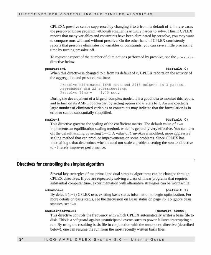
CPLEX’s presolve can be suppressed by changing i to 0 from its default of 1. In rare cases the presolved linear program, although smaller, is actually harder to solve. Thus if CPLEX reports that many variables and constraints have been eliminated by presolve, you may want to compare runs with and without presolve. On the other hand, if CPLEX consistently reports that presolve eliminates no variables or constraints, you can save a little processing time by turning presolve off.
To request a report of the number of eliminations performed by presolve, see the prestats directive below.
prestats=i (default 0)When this directive is changed to 1 from its default of 0, CPLEX reports on the activity of the aggregation and presolve routines:
Presolve eliminated 1645 rows and 2715 columns in 3 passes.Aggregator did 22 substitutions.Presolve Time = 1.70 sec.
During the development of a large or complex model, it is a good idea to monitor this report, and to turn on its AMPL counterpart by setting option show_stats to 1. An unexpectedly large number of eliminated variables or constraints may indicate that the formulation is in error or can be substantially simplified.
scale=i (default 0)This directive governs the scaling of the coefficient matrix. The default value of i=0 implements an equilibration scaling method, which is generally very effective. You can turn off the default scaling by setting i=-1. A value of 1 invokes a modified, more aggressive scaling method that can produce improvements on some problems. Since CPLEX has internal logic that determines when it need not scale a problem, setting the scale directive to -1 rarely improves performance.
Directives for controlling the simplex algorithm
Several key strategies of the primal and dual simplex algorithms can be changed through CPLEX directives. If you are repeatedly solving a class of linear programs that requires substantial computer time, experimentation with alternative strategies can be worthwhile.
advance=i (default 1)By default (i=1) CPLEX uses existing basis status information to begin optimization. For more details on basis status, see the discussion on Basis status on page 76. To ignore basis statuses, set i=0.
basisinterval=i (default 50000)This directive controls the frequency with which CPLEX automatically writes a basis file to disk. This is a safeguard against unanticipated events such as power failures interrupting a run. By using the resulting basis file in conjunction with the xxxstart directive (described below), one can resume the run from the most recently written basis files.
34 I L O G A M P L C P L E X S Y S T E M 8 . 0 — U S E R ’ S G U I D E

D I R E C T I V E S F O R C O N T R O L L I N G T H E S I M P L E X A L G O R I T H M
Usin
g C
PL
EX
for
Lin
ear Pro
gram
min
g
crash=i (default 1)This directive governs CPLEX’s procedure for choosing an initial basis, except when the basis is read from a file as specified by the directive readbasis described below. A value of i=0 causes the objective to be ignored in choosing the basis, whereas values of -1 and 1 select two different heuristics for taking the objective into account. The best setting for your purposes will depend on the specific characteristics of the linear programs you are solving, and must be determined through experimentation.
pgradient=i (default 0)This directive governs the primal simplex algorithm’s choice of a "pricing" procedure that determines which variable is selected to enter the basis at each iteration. Your choice is likely to make a substantial difference to the tradeoff between computational time per iteration and the number of iterations. As a rule of thumb, if the number of iterations to solve your linear program exceeds three times the number of constraints, you should consider experimenting with alternative pricing procedures.
The recognized values of i are as follows:
The "reduced cost" procedures are sophisticated versions of the pricing rules most often described in textbooks. The "devex" and "steepest edge" alternatives employ more elaborate computations, which can better predict the improvement to the objective offered by each candidate variable for entering the basis.
Compared to the default of i=0, the less compute-intensive reduced-cost pricing (i= -1) may be preferred if your problems are small or easy, or are unusually dense—say, 20 to 30 nonzeros per column. Conversely, if you have more difficult problems which take many iterations to complete Phase I, consider using devex pricing (i=1). Each iteration may consume more time, but the lower number of total iterations may lead to a substantial overall reduction in time. Do not use devex pricing if your problem has many variables and relatively few constraints, however, as the number of calculations required per iteration in this situation is usually too large to afford any advantage.
If devex pricing helps, you may wish to try steepest-edge pricing (i=2). This alternative incurs a substantial initialization cost, and is computationally the most expensive per iteration, but may dramatically reduce the number of iterations so as to produce the best results on exceptionally difficult problems. The variant using slack norms (i=3) is a compromise that sidesteps the initialization cost; it is most likely to be advantageous for relatively easy problems that have a low number of iterations or time per iteration.
-1 Reduced-cost pricing
0 Hybrid reduced-cost/devex pricing
1 Devex pricing
2 Steepest-edge pricing
3 Steepest-edge pricing with slack initial norms
4 Full reduced-cost pricing
I L O G A M P L C P L E X S Y S T E M 8 . 0 — U S E R ’ S G U I D E 35

D I R E C T I V E S F O R C O N T R O L L I N G T H E S I M P L E X A L G O R I T H M
Full reduced-cost pricing (i=4) is a variant that computes a reduced cost for every variable, and selects as entering variable one having most negative reduced cost (or most positive, as appropriate). Compared to CPLEX’s standard reduced-cost pricing (i=-1), full reduced-cost pricing takes more time per iteration, but in rare cases reduces the number of iterations more than enough to compensate. This alternative is supplied mainly for completeness, as it is proposed in many textbook discussions of the simplex algorithm.
dgradient=i (default 0)This directive governs the dual simplex algorithm’s choice of a "pricing" procedure that determines which variable is selected to leave the basis at each iteration. Your choice is likely to make a substantial difference to the tradeoff between computational time per iteration and the number of iterations. As a rule of thumb, if the number of iterations to solve your linear program exceeds three times the number of constraints, you should consider experimenting with alternative pricing procedures.
The recognized values of i are as follows:
Standard dual pricing (i=1), described in many textbooks, selects as leaving variable one that is farthest outside its bounds. The three "steepest edge" alternatives employ more elaborate computations, which can better predict the improvement to the objective offered by each candidate for leaving variable. The default (i=0) lets CPLEX choose a dual pricing procedure through an internal heuristic based on problem characteristics.
Steepest-edge pricing involves an extra initialization cost, but its extra cost per iteration is much less in the dual simplex algorithm than in the primal. Thus if you find that your problems solve faster using the dual simplex, you should consider experimenting with the steepest-edge procedures. The standard procedure (i=2) and the variant "in slack space" (i=3) have similar computational costs; often their overall performance is similar as well, though one or the other can be advantageous for particular applications. The variant using "unit initial norms" (i=4) is a compromise that sidesteps the initialization cost; it is most likely to be advantageous for relatively easy problems that have a low number of iterations or time per iteration.
pdswitch=i (default 0)This directive determines whether a switch of algorithms will be made when undoing perturbations or shifts that may occur during execution of the primal or dual simplex algorithm. By default, CPLEX automatically decides whether to switch algorithms. Consider setting this directive to 1 if you observe many cycles of removing perturbations or shifts at the end of the optimization. Set it to -1 to inhibit switching.
0 Pricing procedure determined automatically
1 Standard dual pricing
2 Steepest-edge pricing
3 Steepest-edge pricing in slack space
4 Steepest-edge pricing with unit initial norms
36 I L O G A M P L C P L E X S Y S T E M 8 . 0 — U S E R ’ S G U I D E

D I R E C T I V E S F O R C O N T R O L L I N G T H E S I M P L E X A L G O R I T H M
Usin
g C
PL
EX
for
Lin
ear Pro
gram
min
g
pricing=i (default 0)To promote efficiency, when using reduced-cost pricing in primal simplex, CPLEX considers only a subset of the nonbasic variables as candidates to enter the basis. The default of i=0 selects a heuristic that dynamically determines the size of the candidate list, taking problem dimensions into account. You can manually set the size of this list to i>0, but only very rarely will this improve performance.
refactor=i (default 0)This directive specifies the number of iterations between refactorizations of the basis matrix.
At the default setting of i=0, CPLEX automatically calculates a refactorization frequency by a heuristic formula. You can determine the frequency that CPLEX is using by setting the display directive (described below) to 1. Since each update to the factorization uses more memory, CPLEX may reduce the factorization frequency if memory is low. In extreme cases, the basis may have to be refactored every few iterations and the algorithm will be very slow.
Given adequate memory, CPLEX’s performance is relatively insensitive to changes in refactorization frequency. For a few extremely large, difficult problems you may be able to improve performance by reducing i from the value that CPLEX chooses.
netfind=i (default 1)This directives governs the method used by the CPLEX network optimizer to extract a network from the linear program. The value of i influences the size of the network extracted, potentially reducing optimization time. The default value (i=1) extracts only the natural network from the problem. CPLEX then invokes its network simplex method on the extracted network. In some cases, CPLEX can extract a larger network by multiplying rows by -1 (reflection scaling) and rescaling constraints and variables so that more matrix coefficients are plus or minus 1. Setting the netfind directive to 2 enables reflection scaling only, while setting it to 3 allows reflection scaling and general scaling.
simthreads=i (default 1)This directive only applies to users of parallel CPLEX solvers. It specifies the number of parallel processes used during the simplex method optimization. The dual simplex method can exploit parallel processing (on certain platforms), while the primal simplex method cannot.
xxxstart=i (default 0)Set this parameter to 1 to instruct CPLEX to start the optimization from one of the .xxx format basis files generated by CPLEX when it last solved this problem (see the description of the basisinterval directive above for more information). Note that these .xxx format files are for the presolved problem, so one should not specify .xxx files in readbasis and writebasis directives.
I L O G A M P L C P L E X S Y S T E M 8 . 0 — U S E R ’ S G U I D E 37
D I R E C T I V E S F O R C O N T R O L L I N G T H E B A R R I E R A L G O R I T H M
Directives for controlling the barrier algorithm
Several key strategies of the barrier algorithm can be changed through CPLEX directives. If you are repeatedly solving a class of linear programs that requires substantial computer time, experimentation with alternative strategies can be worthwhile.
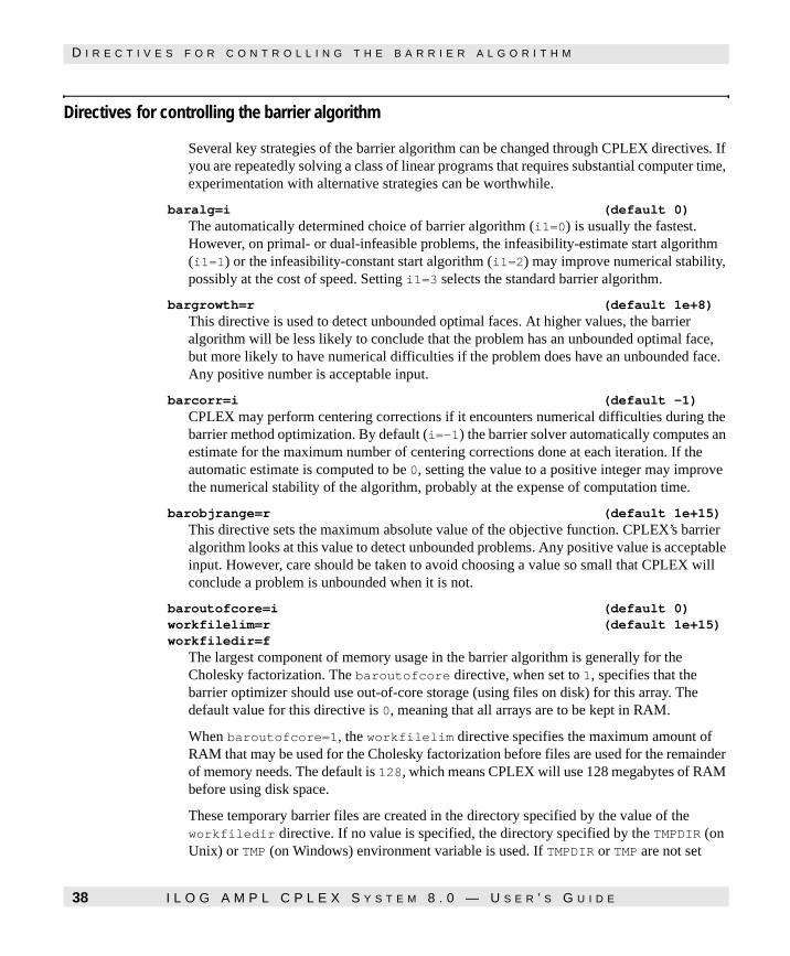
baralg=i (default 0)The automatically determined choice of barrier algorithm (i1=0) is usually the fastest. However, on primal- or dual-infeasible problems, the infeasibility-estimate start algorithm (i1=1) or the infeasibility-constant start algorithm (i1=2) may improve numerical stability, possibly at the cost of speed. Setting i1=3 selects the standard barrier algorithm.
bargrowth=r (default 1e+8)This directive is used to detect unbounded optimal faces. At higher values, the barrier algorithm will be less likely to conclude that the problem has an unbounded optimal face, but more likely to have numerical difficulties if the problem does have an unbounded face. Any positive number is acceptable input.
barcorr=i (default -1)CPLEX may perform centering corrections if it encounters numerical difficulties during the barrier method optimization. By default (i=-1) the barrier solver automatically computes an estimate for the maximum number of centering corrections done at each iteration. If the automatic estimate is computed to be 0, setting the value to a positive integer may improve the numerical stability of the algorithm, probably at the expense of computation time.
barobjrange=r (default 1e+15)This directive sets the maximum absolute value of the objective function. CPLEX’s barrier algorithm looks at this value to detect unbounded problems. Any positive value is acceptable input. However, care should be taken to avoid choosing a value so small that CPLEX will conclude a problem is unbounded when it is not.
baroutofcore=i (default 0)workfilelim=r (default 1e+15)workfiledir=f
The largest component of memory usage in the barrier algorithm is generally for the Cholesky factorization. The baroutofcore directive, when set to 1, specifies that the barrier optimizer should use out-of-core storage (using files on disk) for this array. The default value for this directive is 0, meaning that all arrays are to be kept in RAM.
When baroutofcore=1, the workfilelim directive specifies the maximum amount of RAM that may be used for the Cholesky factorization before files are used for the remainder of memory needs. The default is 128, which means CPLEX will use 128 megabytes of RAM before using disk space.
These temporary barrier files are created in the directory specified by the value of the workfiledir directive. If no value is specified, the directory specified by the TMPDIR (on Unix) or TMP (on Windows) environment variable is used. If TMPDIR or TMP are not set
38 I L O G A M P L C P L E X S Y S T E M 8 . 0 — U S E R ’ S G U I D E

D I R E C T I V E S F O R C O N T R O L L I N G T H E B A R R I E R A L G O R I T H M
Usin
g C
PL
EX
for
Lin
ear Pro
gram
min
g
either, the current working directory is used. Temporary barrier files are deleted automatically when CPLEX terminates normally.
barstart=i (default 1)This directive controls the starting point CPLEX uses to initiate the barrier method. The default setting of 1 will suffice for most problems. Consider other values (2, 3, and 4) if the barrier method appears to converge slowly, or when the predual directive is specified.
barthreads=i (default 1)This directive only applies to users of parallel CPLEX solvers. It specifies the number of parallel processes used during the barrier method optimization.
barvarup=r (default 1e+20)This directive sets the upper bound for all variables that have infinite upper bounds. It is used to prevent difficulties associated with unbounded optimal faces. Any positive value less then or equal to 1e+20 is acceptable input. However, care should be taken to avoid choosing a value so small that CPLEX concludes that a problem has an unbounded optimal face when it does not.
comptol=r (default 1e-8)This directive specifies the complementarity tolerance used by the barrier algorithm to test convergence. The barrier algorithm will terminate with an optimal solution if the relative complementarity is smaller than this value. Any positive number larger than 1e-10 is acceptable input.
crossover=i (default 1)On a linear problem, by default (i=1) CPLEX initiates the "crossover" algorithm to convert the barrier solution to a basic (or vertex) solution using a primal simplex-like method. If i=2, a dual simplex-like method is used for the crossover. The crossover algorithm can be turned off by setting i=0.
densecol=i (default 0)CPLEX uses this directive to distinguish dense columns in the constraint matrix. Because barrier algorithm performance can improve dramatically if dense columns are treated separately, changing this value may improve optimization time. Columns with more nonzeros than this setting are considered to be dense. If left at the default value, CPLEX will automatically determine a value, considering factors such as the size of the problem. Any nonnegative integer is acceptable input.
ordering=i (default 0)This directive selects the method used to permute the rows of the constraint matrix in order to reduce fill in the Cholesky factor. There is a trade-off between ordering speed and sparsity of the Cholesky factor. The automatic default setting usually chooses the best ordering for the problem.
The approximate minimum degree (AMD) algorithm (i=1) balances speed and fill. The approximate minimum fill (AMF) algorithm (i=2) usually generates slightly better orderings than AMD, at the cost of more ordering run-time. The nested dissection (ND)
I L O G A M P L C P L E X S Y S T E M 8 . 0 — U S E R ’ S G U I D E 39

D I R E C T I V E S F O R I M P R O V I N G S T A B I L I T Y
algorithm, triggered by using i=3 sometimes reduces Barrier run-time dramatically—ten-fold reductions have been observed for some problems. This option sometimes produces worse orderings, though, and it requires much more ordering run-time.
Directives for improving stability
CPLEX is highly robust and has been designed to avoid problems such as degenerate stalling and numerical inaccuracy that can occur in the simplex algorithm. However, some linear programs can benefit from adjustments to the following directives if difficulties are encountered.
doperturb=i1 (default 0)perturbation=r (default 1.0e-6)perturblimit=i2 (default 0)
The simplex algorithm tends to make very slow progress when it encounters solutions that are highly degenerate (in the sense of having many basic variables lying at one of their bounds, rather than between them). When CPLEX detects degenerate stalling, it automatically introduces a perturbation that expands the bounds on every variable by a small amount, thereby creating a different but closely related problem. Generally, CPLEX can make faster progress on this less constrained problem; once optimality is indicated, the perturbation is removed by resetting the bounds to their original values.
The value of r determines the size of the perturbation. If you receive messages from CPLEX indicating that the linear program has been perturbed more than once, r is probably too large; reduce it to a level where only one perturbation is required.
The default doperturb value of i1=0 selects CPLEX's automatic perturbation strategy. If an automatic perturbation occurs early in the solution process, consider setting i1=1 to select perturbation at the outset. This alternative will save the time of first allowing the optimization to stall before activating the perturbation mechanism, but is useful only rarely, for extremely degenerate problems.
The perturblimit parameter governs the number of stalled iterations CPLEX allows before perturbing the problem. The default value of i2=0 causes CPLEX to determine this number based on the characteristics of the particular problem being solved. Setting i2 to a positive integer value identifies a specific number of stalled iterations to tolerate before perturbing the problem.
feasibility=r1 (default 1.0e-6)markowitz=r2 (default 0.01)optimality=r3 (default 1.0e-6)
If a problem is making slow progress through Phase I, or repeatedly becomes infeasible during Phase II, numerical difficulties have arisen. Adjusting the algorithmic tolerances controlled by these directives may help. Decreasing the feasibility tolerance, increasing the
40 I L O G A M P L C P L E X S Y S T E M 8 . 0 — U S E R ’ S G U I D E

D I R E C T I V E S F O R S T A R T I N G A N D S T O P P I N G
Usin
g C
PL
EX
for
Lin
ear Pro
gram
min
g
optimality tolerance and/or increasing the Markowitz tolerance will typically improve numerical behavior.
The feasibility tolerance r1>0 specifies the degree to which a linear program’s basic variables may violate their bounds. You may wish to lower r1 after finding an optimal solution if there is any doubt that the solution is truly optimal; but if it is set too low, CPLEX may falsely conclude that the problem has no feasible solution. Valid values for r1 lie between 1e-9 and 0.1.
The Markowitz threshold r2<1 influences the order in which variables are eliminated during basis factorization. Increasing r2 may yield a more accurate factorization, and consequently more accurate computations during iterations of the simplex algorithm. Too large a value may produce an inefficiently dense factorization, however. Valid values for r2 lie between 0.0001 and 0.99999.
The optimality tolerance r3>0 specifies how closely the optimality (or dual feasibility) conditions must be satisfied for CPLEX to declare an optimal solution. Valid values for r3 lie between 1e-9 and 0.01.
Directives for starting and stopping
Normally CPLEX uses an internal procedure to determine a starting point for the simplex algorithm, then iterates to optimality. The following directives override these conventions so that you can start from a saved basis, and can stop when a certain criterion is satisfied.
Command-line versions of CPLEX for AMPL can also be stopped by using break, typically by pressing the Control and C keys simultaneously. The best solution found so far is returned.
bariterlim=i (default 2100000000)CPLEX stops after i barrier method iterations and returns its current solution, whether or not it has determined that the solution is optimal.
clocktype=i (default 1)The default setting of clocktype=1 means that CPLEX will measure time in terms of CPU seconds. A setting of 2 means that CPLEX will measure time in terms of elapsed wall-clock seconds.
lpiterlim=i (default 2.1e+9 or larger)CPLEX stops after i simplex method iterations and returns its current solution, whether or not it has determined that the solution is optimal.
lowerobj=r1 (default -1.0e+75)upperobj=r2 (default +1.0e+75)
CPLEX stops at the first iteration where the solution is feasible in the constraints, and the objective value is below r1 or above r2. At their default values these directives have no
I L O G A M P L C P L E X S Y S T E M 8 . 0 — U S E R ’ S G U I D E 41

D I R E C T I V E S F O R S T A R T I N G A N D S T O P P I N G
practical effect. Setting r1 (for a minimization) or r2 (for a maximization) to a "good" value for the objective will cause CPLEX to stop as soon as it achieves this value.
readbasis=f1writebasis=f2
Current versions do not require you to explicitly save the basis to hot-start CPLEX - variable status is automatically stored and used between CPLEX invocations. The readbasis and writebasis directives are included for backward compatibility with previous versions of CPLEX for AMPL, which did not use variable status information.
If the readbasis directive is specified, then the initial basis is instead read from the file f1, which must also be in the standard MPS basis format. This basis determines the initial solution.
If the writebasis directive is specified, CPLEX writes a record of the final simplex basis to the file named f2, in the standard MPS basis format. Normally this is an optimal basis, but it may be otherwise if an optimum does not exist or could not be found by the chosen algorithm, or if the iterations were terminated prematurely by one of the directives described below.
readvector=f1writevector=f2
These directives are used to take a barrier algorithm solution and write it to or read it from a CPLEX .vec file. Because AMPL always instructs CPLEX to take its barrier method solution and apply a hybrid method to obtain a basic solution, this feature can only be used if a barrier iteration limit is exceeded.
If the readvector directive is specified, CPLEX will read in a .vec file named f1 and use it to initiate the hybrid crossover method that results in an optimal basic solution. Note that CPLEX will not perform additional barrier iterations after reading in the .vec file. Similarly, if the writevector directive is specified, CPLEX will write out .vec file named f2.
singular=i (default 10)CPLEX will attempt to repair the basis matrix up to i times when it finds evidence that the matrix is singular. Once this limit is exceeded, CPLEX terminates with the current basis set to the best factorizable basis that has been found.
timelimit=r (default 1.0e+75)CPLEX stops after r seconds of computation time and returns its current solution, whether or not it has determined that the solution is optimal.
42 I L O G A M P L C P L E X S Y S T E M 8 . 0 — U S E R ’ S G U I D E

D I R E C T I V E S F O R C O N T R O L L I N G O U T P U T
Usin
g C
PL
EX
for
Lin
ear Pro
gram
min
g
Directives for controlling output
When invoked by solve, CPLEX normally returns just a few lines to your screen to summarize its performance. The following directives let you choose a greater amount of output, which may be useful for monitoring the progress of a long run or for comparing the effects of other directives on the detailed behavior on CPLEX’s algorithms. Output normally comes to the screen, but it may be redirected to a file by specifying solve >filename.
bardisplay=i (default 0)The default choice of i=0 produces a minimal few lines of output from CPLEX, summarizing the results of a barrier method run.
When i=1, a log line recording the barrier iteration number, primal and dual objective values, and infeasibility information is displayed after each barrier iteration.
When i=2, additional information about the barrier run is provided. This level of output is occasionally useful for diagnosing problems of degeneracy or instability in the barrier algorithm.
file=f1This directive instructs CPLEX to write a copy of the model it receives for solution into a file named f1.
iisfind=i (default 0)When i=1 for an infeasible problem, CPLEX returns an irreducible infeasible subset (IIS) of the constraints and variable bounds. By definition, members of an IIS have no feasible solution, but dropping any one of them permits a solution to be found to the remaining ones. Clearly, knowing the composition of an IIS can help localize the source of the infeasibility.
Setting i=2 generates a potentially smaller IIS, at the cost of greater computation time. When iisfind is used, CPLEX uses the .iis suffix to specify which variables and constraints are in the IIS, as explained in Diagnosing infeasibilities on page 68.
logfile=f1This directive instructs CPLEX to create a log file named f1 that will contain output from the optimization. The amount of output in the log file will depend on other directives, such as the display directive described above.
lpdisplay=i (default 0)The default choice of i=0 produces a minimal few lines of output from CPLEX, summarizing the results of the run.
When i=1, a log line recording the iteration number and the scaled infeasibility or objective value is displayed after each refactorization of the basis matrix. Additional information on the operation of the network simplex algorithm is also provided, if applicable. This is often the appropriate setting for tracking the progress of a long run.
I L O G A M P L C P L E X S Y S T E M 8 . 0 — U S E R ’ S G U I D E 43

D I R E C T I V E S F O R C O N T R O L L I N G O U T P U T
When i=2, a log line is displayed after each iteration. This level of output is occasionally useful for diagnosing problems of degeneracy or instability in the simplex algorithm.
sensitivityWhen specified, this directive instructs CPLEX to output sensitivity ranges corresponding to the optimal solution. For variables, the suffix .current provides the corresponding objective function coefficient in the current problem, and .down and .up specify the smallest and largest values for which the current basis remains optimal. For constraints, the suffixes apply to the constant value, or right-hand-side. Details on CPLEX-defined suffixes are provided in Defined Suffixes for CPLEX on page 65.
timing=i (default 0)When this directive is changed to 1 from its default value of 0, a summary of processing times is displayed to "standard output":
Input = 0.06 CPU 0.06 Wall
Solve = 6.42 CPU 6.42 Wall
Output = 0.05 CPU 0.05 Wall
Input is the time that CPLEX takes to read the problem from a file that has been written by AMPL. Solve is the time that CPLEX spends trying to solve the problem. Output is the time that CPLEX takes to write the solution to a file for AMPL to read. CPU values provide processor time, whereas Wall values provide elapsed time.
Setting i=2 writes the timing information to "standard error", and setting i=3 directs the information to both the standard output and the standard error. The latter two options are only interesting for Unix CPLEX for AMPL users.
versionThis directive causes the display of the CPLEX version being used to solve the problem.
44 I L O G A M P L C P L E X S Y S T E M 8 . 0 — U S E R ’ S G U I D E

C H A P T E R
Usin
g C
PL
EX
for
Integ
er Pro
gram
min
g
7
Using CPLEX for Integer Programming
CPLEX mixed integer algorithm
For problems that contain integer variables, CPLEX uses a branch & bound approach. The optimizing algorithm maintains a hierarchy of related linear programming subproblems, referred to as the search tree and usually visualized as branching downward:
There is a subproblem at each node of the tree, and each node is explored by solving the associated subproblem.
The algorithm starts with just a top (or root) node, whose associated subproblem is the relaxation of the integer program—the LP that results when all integrality restrictions are
I L O G A M P L C P L E X S Y S T E M 8 . 0 — U S E R ’ S G U I D E 45

C P L E X M I X E D I N T E G E R A L G O R I T H M
dropped. If this relaxation happened to have an integer solution, then it would provide an optimal solution to the integer program. Normally, however, the optimum for the relaxation has some fractional-valued integer variables. A fractional variable is then chosen for branching, and two new subproblems are generated, each with more restrictive bounds for the branching variable. For example, if the branching variable is binary (or 0–1), one subproblem will have the variable fixed at zero, the other node will have it fixed at one. In the search tree, the two new subproblems are represented by two new nodes connected to the root. Most likely each of these subproblems also has fractional-valued integer variables, in which case the branching process must be repeated; successive branchings produce the tree structure shown above.
If there are more than a few integer variables, the branching process has the potential to create more nodes than any computer can hold. There are two key circumstances, however, in which branching from a particular node can be discontinued:
◆ The node’s subproblem has no fractional-valued integer variables. It thus provides a feasible solution to the original integer program. If this solution yields a better objective value than any other feasible solution found so far, it becomes the incumbent, and is saved for future comparison.
◆ The node’s subproblem has no feasible solution, or has an optimum that is worse than a certain cutoff value. Since any subproblems under this node would be more restricted, they would also either be infeasible or have an optimum value worse than the cutoff. Thus none of these subproblems need be considered.
In these cases the node is said to be fathomed. Because subproblems become more restricted with each branching, the likelihood of fathoming a node becomes greater as the algorithm gets deeper into the tree. So long as nodes are not created by branching much faster than they are inactivated by fathoming, the tree can be kept to a reasonable size.
When no active nodes are left, CPLEX is finished, and it reports the final incumbent solution back to AMPL. If the cutoff value has been set throughout the algorithm to the objective value of the current incumbent—CPLEX's default strategy—then the reported solution is declared optimal. Other cutoff options, described below, cannot provide a provably optimal solution, but may allow the algorithm to finish much faster.
CPLEX's memory requirement for solving linear subproblems is about the same as its requirement for linear programs discussed in the previous section. In the branch & bound algorithm, however, each active node of the tree requires additional memory. The total memory that CPLEX needs to prove optimality for an integer program can thus be much larger and less predictable than for a linear program of comparable size.
Because a single integer program generates many LP subproblems, even small instances can be very computation-intensive and require significant amounts of memory. In contrast to solving linear programming problems, where little user intervention is required to obtain optimal results, you may have to set some of the following directives to get satisfactory results on integer programs. You can either change the way that the branch & bound
46 I L O G A M P L C P L E X S Y S T E M 8 . 0 — U S E R ’ S G U I D E

Usin
g C
PL
EX
for
Integ
er Pro
gram
min
gD I R E C T I V E S F O R P R E P R O C E S S I N G
algorithms work, or relax the conditions for optimality, as explained in the two corresponding subsections below. When experimenting with these possibilities, it is also a good idea to include directives that set stopping criteria and display informative output; these are described in the next two subsections. If you consistently fail to receive any useful solution in response to the solve command after a reasonable amount of time, and are in doubt as to how to proceed, consult the troubleshooting tips at the end of this section.
Directives for preprocessing
All of the preprocessing directives described in Using CPLEX for Linear Programming are also applicable to problems that specify integer-valued variables. The following directives control additional preprocessing steps that are applicable to certain mixed integer programs only.
aggcutlim=i (default 3)This directive controls the number of constraints that can be aggregated for generating flow cover and mixed integer rounding cuts. In most cases the default setting of 3 will be satisfactory. Set it to 0 to prevent any aggregation.
boundstr=i (default -1)Bound strengthening tightens the bounds on variables in mixed integer programs. This may enable CPLEX to fix the variable and remove it from consideration during the branch & bound algorithm. By default (i=-1), CPLEX automatically decides whether to perform bound strengthening. This reduction usually improves performance, but occasionally takes a long time, due to its iterative nature. In cases where the time required for bound strengthening outweighs any subsequent reduction in run time, disable this feature by setting i=0. To turn on bound strengthening, set i=1.
mipcuts=i (default 0)or
cliquecuts=i1 (default 0)covercuts=i2 (default 0)disjcuts=i3 (default 0)flowcuts=i4 (default 0)flowpathcuts=i5 (default 0)fraccuts=i6 (default 0)gubcuts=i7 (default 0)impliedcuts=i8 (default 0)mircuts=i9 (default 0)
Integer programming solve times can often be improved by generating new constraints (or cuts) based on polyhedral considerations. These additional constraints tighten the feasible region, reducing the number of fractional variables to choose from when CPLEX needs to select a branching variable. CPLEX can generate cuts based on different combinatorial constructs corresponding to the directives listed above.
I L O G A M P L C P L E X S Y S T E M 8 . 0 — U S E R ’ S G U I D E 47

D I R E C T I V E S F O R P R E P R O C E S S I N G
By default, CPLEX decides whether to generate cuts. Typically the default setting yields the best performance. To disable a particular family of cuts, set its directive to -1. To enable moderate cut generation, set the appropriate directive to 1. To enable aggressive cut generation, set it to 2. To set all these classes of cuts to one common value, for instance -1 to disable all cuts, use the directive mipcuts. Cuts directives are applied in the order in which they are encountered, so for instance mipcuts=-1 fraccuts=2 first turns off all cuts and then turns fractional cuts back on. The reverse cae of fraccuts=2 mipcuts=-1 results in all cuts being disabled as though the fraccuts=2 directive is not present.
Using more aggressive cut generation causes CPLEX to make more passes through the problem to generate cuts. The disjcuts directive also supports a setting of 3 for very aggressive cut generation.
coeffreduce=i (default 2)Coefficient reduction during the presolve phase typically improves CPLEX’s performance on integer programs by speeding up the solve times of the LP subproblems solved in the branch-and-bound algorithm. However, while coefficient reduction will tighten the LP subproblems, occasionally it makes them more difficult to solve. So, if CPLEX solves an integer program in a modest number of nodes, but the LP subproblem at each node consumes significant amounts of time, solve time may improve by setting i=0 to disable this feature. The node count may increase, but the savings in time per node may compensate for the increased node count. The default setting of i=2 causes CPLEX to perform coefficient reduction whenever possible, while i=1 will only reduce coefficients to integer values.
cutpass=i (default 0)This directive controls the number of passes CPLEX performs when generating cutting planes for a MIP model. By default, CPLEX automatically determines the number of passes to perform. This setting should suffice for most problems. Set the cutpass directive to -1 to stop all cut generation. Set it to a positive integer to specify a particular number of passes.
cutsfactor=r (default 4.0)The cutsfactor directive controls the number of additional cuts generated by CPLEX. While the constraints generated by CPLEX improve performance in most cases, in some problems the additional memory to store them and time required to solve the larger LP subproblems may outweigh the performance gains from the tighter problem formulation. In such cases, use this directive to limit the number of cuts that CPLEX generates. CPLEX will generate no more than r times the number of rows in the problem.
fraccand=i (default 200)This directive limits the number of candidate variables CPLEX will examine when generating fractional cuts on a MIP model. For most purposes the default of 200 will be satisfactory.
fracpass=i (default 0)This directive controls the number of passes CPLEX performs when generating fractional cuts on a MIP model. The default of 0 instructs CPLEX to automatically determine the
48 I L O G A M P L C P L E X S Y S T E M 8 . 0 — U S E R ’ S G U I D E

Usin
g C
PL
EX
for
Integ
er Pro
gram
min
gD I R E C T I V E S F O R P R E P R O C E S S I N G
number of passes and should suffice for most problems. Set it to a positive integer to specify a particular number of passes.
mipstartstatus=i1 (default 1)mipstartvalue=i2 (default 1)
These directives control how existing MIP solution information is used by CPLEX. The default value of i1=1 tells CPLEX to use incoming variable and constraint statuses. Incoming statuses can be ignored by setting i1=0.
Note however, that mipstartstatus is normally overridden by the AMPL option send_statuses, which can take on the following values:
By default (i2=1) variable values are checked to see if they provide an integer feasible solution before the problem is optimized. If an integer feasible solution is found, the objective function value is used as a cutoff during branch & bound. To ignore existing values, set i2=0.
prerelax=i (default 0)Setting i=1 invokes the CPLEX presolve for the linear program associated with the initial relaxation of a mixed integer program. All other presolve settings apply. Sometimes additional reductions can be made beyond any previously performed MIP presolve reductions.
presolvenode=i (default 0)The presolvenode directive determines how CPLEX applies its presolve to the LP subproblems at the nodes of the branch and bound tree. By default, CPLEX decides automatically. Set i=1 to force node presolve. Set i=-1 to prevent it. The default setting usually works best.
probe=i (default 0)This directive controls whether CPLEX should perform probing before solving the MIP. Probing can lead to dramatic reductions in the problem size, but can also consume large amounts of time. By default (i=0) CPLEX automatically decides whether to perform probing. To disable probing, set i=-1. To enable probing, set it to a value of 1, 2 or 3. A larger value results in an increased level of probing. More probing can lead to greater reductions in problem size, but also significant increases in probing time.
sos1=i (default 1)An optimization problem containing restrictions that at most one of a specified group of variables can take a nonzero value is a form of discrete optimization that can be handled by an equivalent mixed integer program. When i is at its default value of 1, this conversion is
0 ⇒ send no solver status values
1 (default) ⇒ send statuses if there are no integer variables
2 ⇒ send statuses even if there are integer variables.
I L O G A M P L C P L E X S Y S T E M 8 . 0 — U S E R ’ S G U I D E 49

D I R E C T I V E S F O R A L G O R I T H M I C C O N T R O L
performed using a structure known as a special ordered set (of type 1). If i is changed to 0, the conversion is made instead to an equivalent formulation using multiple binary variables.
sos2=i (default 1)An optimization problem containing piecewise-linear terms may have to be converted to an equivalent mixed integer program, as explained in Piecewise-linear programs on page 24. When i is at its default value of 1, this conversion results in only one extra variable per piecewise-linear breakpoint. All of the extra variables associated with a particular piecewise-linear term are marked as belonging together, so that CPLEX’s branch & bound procedure knows to treat them specially. Variables so marked have come to be known as a special ordered set of type 2, whence the name sos2 for this directive.
When i is changed to 0 from its default of 1, the conversion creates a larger number of variables, but does not employ the special ordered set feature. This alternative has no known advantages, and is supplied for completeness only.
Directives for algorithmic control
CPLEX has default values for the algorithmic control directives that often work well for solving a wide range of mixed integer programs. However, it is sometimes necessary to specify alternative values for one or more of the following directives to improve solution times.
You can view each of these directives as corresponding to a particular decision faced at each step in the branch & bound procedure. To be specific, imagine that an LP subproblem has just been solved. The sequence of decisions and the corresponding directives are then as follows:
◆ Branch next from which node in the tree? (backtrack, nodesel)
◆ Branch by constraining which fractional variable at the selected node? (mip_priorities, ordertype, varselect; refer to the discussion on setting priorities by variable in Algorithmic control on page 65.)
◆ Investigate which of a fractional variable’s two resulting branches first? (branch; refer to the discussion on setting branching preference by variable in Algorithmic control on page 65.)
◆ Solve the resulting new subproblem by which LP algorithm? (mipalgorithm)
◆ Explore rounded subproblem solutions how often? (heuristicfreq)
It is often hard to predict which combination of directives will work best. Some experimentation is usually required; your knowledge of the problem structure may also suggest certain choices of branch & bound strategy.
50 I L O G A M P L C P L E X S Y S T E M 8 . 0 — U S E R ’ S G U I D E

Usin
g C
PL
EX
for
Integ
er Pro
gram
min
gD I R E C T I V E S F O R A L G O R I T H M I C C O N T R O L
backtrack=r (default 0.9999)bbinterval=i1 (default 7)nodeselect=i2 (default 1)
These directives determine the criterion for choosing the next node from which to branch, once a feasible integer solution has been found.
Depending on whether i2 is set to 1, 2, or 3, CPLEX associates a value with each node and chooses a node based on these values. For i2=1, a node’s value is the bound on the integer optimum that is given by solving the LP subproblem at that node. For i2=2 or i2=3, a node’s value is an estimate of the best integer objective that can be achieved by branching from that node; estimates of node objective values are derived from so-called pseudocosts, which are in turn derived from the solutions to the LP subproblems. Settings 2 and 3 differ regarding the exact nature of the estimated objective. Depending on the value at the current (most recently created) active node, CPLEX either branches from that node, or else backtracks to the node that has the best bound (i2=1) or best estimate (i2=2 or i2=3) among all active nodes.
When used in conjunction with best estimate node selection (i2=2), the bbinterval setting (i1) controls the interval for selecting the best bound node. Decreasing this interval may be useful when best estimate finds good solutions but makes little progress moving the bound. Conversely, increasing i1 may help when the best estimate node selection does not find any good integer solutions.
The backtracking decision is made by comparing the value (bound or estimate) at the current node with the values at parent nodes in the tree. If the value of the current node has degraded (increased for a minimization, decreased for a maximization) by at least a certain amount relative to the values at parent nodes, then a backtrack is performed. The cutoff for degradation is determined by an internal heuristic that is regulated by the value of r.
Lower values of r (which can range from 0 to 1) favor backtracking, resulting in a strategy that is more nearly "breadth first". The search jumps around fairly high in the tree, solving somewhat dissimilar subproblems. Good solutions are likely to be found sooner through this strategy, but the processing time per node is also greater.
Higher values of r discourage backtracking, yielding a strategy that is more nearly "depth first". Successive subproblems are more similar, nodes are processed faster, and integer solutions are often quickly found deep in the search tree. Considerable time may be wasted in searching the descendants of one node, however, before backtracking to a better part of the tree.
The default value of .01 gives a moderately breadth-first search and represents a good compromise. Lower values often pay off when the LP subproblems are expensive to solve.
Setting i2 to 0 chooses a pure depth-first strategy, regardless of r. CPLEX automatically uses this strategy to search for an initial feasible integer solution at the outset of the branch & bound procedure.
I L O G A M P L C P L E X S Y S T E M 8 . 0 — U S E R ’ S G U I D E 51

D I R E C T I V E S F O R A L G O R I T H M I C C O N T R O L
branch=i1 (default 0)The branch directive determines the direction in which CPLEX branches on the selected fractional variable. When branching on a variable x that has fractional value r, CPLEX creates one subproblem that has the constraint x>ceil(r) and one that has the constraint x<floor(r); these are the "up branch" and "down branch" respectively. By default (i1=0), CPLEX uses an internal heuristic to decide whether it should first process the subproblem on the up branch or on the down branch. You may instead specify consistent selection of the up branch (i1=1) or down branch (i1= -1). Sometimes one of these settings leads the algorithm to examine and discard the "poorer" branches high in the tree, reducing the tree size and overall solution time. Branching control can also be exercised using the .direction suffix described in Algorithmic control on page 65.
heuristicfreq=i3 (default 0)Use the heuristicfreq directive to specify the frequency with which CPLEX applies a rounding heuristic at the nodes. This can help find solutions missed using other settings. The default value (i3=0) instructs CPLEX to use internal logic to decide when to apply the heuristic. To suppress application of the heuristic at all nodes, let i3=-1. To specify the node frequency with which CPLEX applies the heuristic, set i3 to a positive integer.
mipalgorithm=i1 (default 2)mipcrossover=i2 (default 1)
This directive specifies the algorithm, or combination of algorithms, that CPLEX will apply to solve the LP subproblem at each branch & bound node. The recognized values of i1 are:
The default strategy uses an internal heuristic to determine when to switch from dual to primal simplex. It usually performs well, but the other strategies can significantly reduce the time per node. These settings do not significantly affect the number of nodes that must be visited during the search.
When the Barrier algorithm is used to solve subproblems (i1=4), by default (i2=1) CPLEX uses primal simplex for the crossover. In certain cases, dual simplex (i2=2) may be faster.
option mip_priorities ’v1 i1 v2 i2 ...’ ;From CPLEX 7.0 onwards, the mip_priorities option has been superseded by the .priority suffix. Please refer to Algorithmic control on page 65 for a discussion of setting priorities by individual variable.
mipemphasis=i (default 0)This directive guides CPLEX’s branch & bound strategy. The default of 0 corresponds to a balance between searching for feasible solutions and proving optimality, and works well for most users’ purposes. A setting of 1 shifts the emphasis strongly toward finding new feasible
1 Primal simplex
2 Dual simplex
3 Network simplex
4 Barrier
5 Sifting
52 I L O G A M P L C P L E X S Y S T E M 8 . 0 — U S E R ’ S G U I D E

Usin
g C
PL
EX
for
Integ
er Pro
gram
min
gD I R E C T I V E S F O R A L G O R I T H M I C C O N T R O L
solutions, and may be an appropriate setting with difficult models for which a proof of optimality is unlikely to be reached anyway. A setting of 2 shifts the emphasis slightly more toward the proof of optimality and away from finding new feasibles. A setting of 3 shifts the emphasis very aggressively toward the optimality proof by concentrating on moving the best bound value, and may be an appropriate setting for models resistant to other solution techniques or when feasible solutions without a proof of optimality are of no value. None of these emphasis settings changes the fundamental nature of the CPLEX branch & bound algorithm, which is to deliver proved optimal solutions if given enough time; the setting merely changes some internal strategies and tactics along the way, and represents a way for the user to express his or her aims in a way that is separate from the model formulation.
mipthreads=i (default 1)This directive only applies to users of parallel CPLEX solvers. It specifies the number of parallel processes used during the branch & bound optimization.
nodefile=i (default 1)workfilelim=r (default 128)workfiledir=f
The list of unprocessed nodes in the branch & bound tree typically dominates CPLEX’s memory usage when solving integer programs. A setting of 0 for the nodefile directive causes CPLEX to store all nodes in physical memory. The default value of 1 creates a compressed version of the node file in memory.
Writing nodes to disk (i=2, 3) enables CPLEX to process more nodes before running out of memory. This is typically more efficient than relying on the operating system’s generic swapping procedure. If i=2, an uncompressed node file is written to disk. Compressing the file (i=3) adds computation time, but allows more efficient use of memory.
When the nodefile directive instructs CPLEX to write nodes to a node file, the workfilelim directive specifies the maximum size of RAM to be consumed before writing to disk takes place. Although node files are designed for efficiency, the speed of RAM is always superior to that of disk, and you should take advantage of what memory your computer has. The default value of 128, a reasonable value for most computers, means that 128 megabytes of RAM will be devoted to storing the tree, and requirements beyond that will begin to go to files on disk. A related directive is treememlim, described below, which serves to place a limit on the total size of the tree. The default value of the treememlim directive is effectively infinity, which means CPLEX will continue to write nodes to disk until it solves the problem, or exhausts available disk space, or encounters some other limit.
Disk node files are created in the temporary directory specified by the value of the workfiledir directive. If no value is specified, the directory specified by the TMPDIR (on Unix) or TMP (on Windows) environment variable is used. If TMPDIR or TMP are not set either, the current working directory is used. Node files are deleted automatically when CPLEX terminates normally.
I L O G A M P L C P L E X S Y S T E M 8 . 0 — U S E R ’ S G U I D E 53
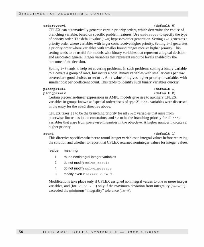
D I R E C T I V E S F O R A L G O R I T H M I C C O N T R O L
ordertype=i (default 0)CPLEX can automatically generate certain priority orders, which determine the choice of branching variable, based on specific problem features. Use ordertype to specify the type of priority order. The default value (i=0) bypasses order generation. Setting i=1 generates a priority order where variables with larger costs receive higher priority. Setting i=2 generates a priority order where variables with smaller bound ranges receive higher priority. This setting tends to be useful for models with binary variables that represent a logical decision and associated general integer variables that represent resource levels enabled by the outcome of the decision.
Setting i=3 tends to help set covering problems. In such problems setting a binary variable to 1 covers a group of rows, but incurs a cost. Binary variables with smaller costs per row covered are good choices to set to 1. An i value of 3 gives higher priority to variables with smaller cost per coefficient count. This tends to identify such binary variables quickly.
plconpri=i1 (default 1)plobjpri=i2 (default 2)
Certain piecewise-linear expressions in AMPL models give rise to auxiliary CPLEX variables in groups known as "special ordered sets of type 2". Sos2 variables were discussed in the entry for the sos2 directive above.
CPLEX takes i1 to be the branching priority for all sos2 variables that arise from piecewise-linearities in the constraints, and i2 to be the branching priority for all sos2 variables that arise from piecewise-linearities in the objective. A higher number indicates a higher priority.
round (default 1)This directive specifies whether to round integer variables to integral values before returning the solution and whether to report that CPLEX returned noninteger values for integer values.
Modifications take place only if CPLEX assigned nonintegral values to one or more integer variables, and (for round < 8) only if the maximum deviation from integrality (maxerr) exceeded the minimum “integrality” tolerance (1e-9).
value meaning
1 round nonintegral integer variables
2 do not modify solve_result
4 do not modify solve_message
8 modify even if maxerr < 1e-9
54 I L O G A M P L C P L E X S Y S T E M 8 . 0 — U S E R ’ S G U I D E

Usin
g C
PL
EX
for
Integ
er Pro
gram
min
gD I R E C T I V E S F O R A L G O R I T H M I C C O N T R O L
startalgorithm=i (default 0)This directive specifies the algorithm that CPLEX will apply to solve the initial LP relaxation. The recognized values of i are:
strongcand=i1 (default 10)strongit=i2 (default 0)strongthreads=i3 (default 1)
These three directives impact strong branching (see varsel directive below).
The strongcand directive controls the size of the candidate list for strong branching. The strongit parameter limits the number of iterations performed on each branch in strong branching. The default setting of i2=0, which allows CPLEX to determine the iteration parameter, will generally suffice. You can use low values of i1 and i2 if the time per strong branching node appears excessive; you may reduce the time per node yet still maintain the performance. Conversely, if the time per node is reasonable but CPLEX makes limited progress, consider increasing the values.
Users of parallel CPLEX can control the number of threads used in strong branching using the strongthreads directive.
varselect=i (default 0)Once a node has been selected for branching, this directive determines how CPLEX chooses a fractional-valued variable to branch on. By default (i=0) the choice is made by an internal heuristic based on the problem and its progress.
The maximum infeasibility rule (i=1) chooses the variable with the largest fractional part. This forces larger changes earlier in the tree, but it tends to disregard the objective function in doing so.
The minimum infeasibility rule (i= -1) chooses the variable with the smallest fractional part. This may lead more quickly to a first integer feasible solution, but will usually be slower overall to reach the optimal integer solution.
A pseudocost rule (i=2) estimates the worsening of the objective that will result by forcing each fractional variable to an adjacent integer, and uses these "degradations" in an internal heuristic for choosing a variable to branch on. This setting tends to be most effective when the problem embodies complex tradeoffs, and the dual variables have an economic interpretation.
0 Automatic
1 Primal simplex
2 Dual simplex
3 Network simplex
4 Barrier
5 Sifting
6 Concurrent
I L O G A M P L C P L E X S Y S T E M 8 . 0 — U S E R ’ S G U I D E 55
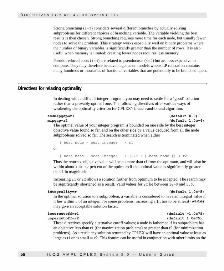
D I R E C T I V E S F O R R E L A X I N G O P T I M A L I T Y
Strong branching (i=3) considers several different branches by actually solving subproblems for different choices of branching variable. The variable yielding the best results is then chosen. Strong branching requires more time for each node, but usually fewer nodes to solve the problem. This strategy works especially well on binary problems where the number of binary variables is significantly greater than the number of rows. It is also useful when memory is limited: creating fewer nodes requires less memory.
Pseudo reduced costs (i=4) are related to pseudocosts (i=2) but are less expensive to compute. They may therefore be advantageous on models whose LP relaxation contains many hundreds or thousands of fractional variables that are potentially to be branched upon.
Directives for relaxing optimality
In dealing with a difficult integer program, you may need to settle for a "good" solution rather than a provably optimal one. The following directives offer various ways of weakening the optimality criterion for CPLEX’s branch-and-bound algorithm.
absmipgap=r1 (default 0.0)mipgap=r2 (default 1.0e-4)
The optimal value of your integer program is bounded on one side by the best integer objective value found so far, and on the other side by a value deduced from all the node subproblems solved so far. The search is terminated when either
| best node - best integer | < r1
or
| best node - best integer | / (1.0 + | best node |) < r2
Thus the returned objective value will be no more than r1 from the optimum, and will also be within about 100 r2 percent of the optimum if the optimal value is significantly greater than 1 in magnitude.
Increasing r1 or r2 allows a solution further from optimum to be accepted. The search may be significantly shortened as a result. Valid values for r2 lie between 1e-9 and 1.0.
integrality=r (default 1.0e-5)In the optimal solution to a subproblem, a variable is considered to have an integral value if it lies within r of an integer. For some problems, increasing r (it has to be at least ✑❅✍✙ ) may give an acceptable solution faster.
lowercutoff=r1 (default -1.0e75)uppercutoff=r2 (default 1.0e75)
These directives specify alternative cutoff values; a node is fathomed if its subproblem has an objective less than r1 (for maximization problems) or greater than r2 (for minimization problems). As a result any solution returned by CPLEX will have an optimal value at least as large as r1 or as small as r2. This feature can be useful in conjunction with other limits on the
56 I L O G A M P L C P L E X S Y S T E M 8 . 0 — U S E R ’ S G U I D E

Usin
g C
PL
EX
for
Integ
er Pro
gram
min
gD I R E C T I V E S F O R H A L T I N G A N D R E S U M I N G T H E S E A R C H
search; but too high a value of r1 or too low a value of r2 may result in no integer solution being found.
objdifference=r1 (default 0.0)relobjdiff=r2 (default 0.0)
This directive automatically updates the cutoff to more restrictive values. Normally the incumbent integer solution’s objective value is used as the cutoff for subsequent nodes. When r1 > 0, the cutoff is instead the incumbent’s value -r1 (if minimizing) or +r1 (if maximizing). This forces the mixed integer optimization to ignore integer solutions that are not at least r1 better than the one found so far. As a result there tend to be fewer nodes generated, and the algorithm terminates more quickly; but the true integer optimum may be missed if its objective value is within r1 of the best integer objective found.
If r1=0, r2 is used to adjust the objective function value during the optimization. For a maximization problem, r2 times the absolute value of the objective function value is added to the best feasible objective value obtained so far. Similarly, if the objective is to be minimized, r2 times the absolute value is subtracted from the best-so-far feasible objective value. Subsequent nodes are ignored if their linear relaxations have optimal values worse that this adjusted value. Positive values of r2 usually speed the search, but may cause the true optimum to be missed.
Directives for halting and resuming the search
There is usually no need to make exhaustive runs to determine the impact of different search strategies or optimality criteria. While you are experimenting, consider using one of the directives below to set a stopping criterion in advance. In each case, the best solution found so far is returned to AMPL. (As mentioned earlier, using "break" on command-line versions of CPLEX for AMPL will return the best known solution - for integer programs, that means the current incumbent.)
You can arrange to save the entire search tree when CPLEX halts, so that the search may be resumed from where it left off. Directives for this purpose are also listed below.
clocktype=i (default 1)The default setting of clocktype=1 means that CPLEX will measure time in terms of CPU seconds. A setting of 2 means that CPLEX will measure time in terms of elapsed wall-clock seconds.
endtree=f1starttree=f2
CPLEX progressively allocates more memory for the search tree as the branch & bound procedure creates new nodes; it frees all this memory at termination. If the endtree directive is specified, CPLEX also writes a record of the final tree to the file named f1, in a compact binary format.
I L O G A M P L C P L E X S Y S T E M 8 . 0 — U S E R ’ S G U I D E 57

D I R E C T I V E S F O R H A L T I N G A N D R E S U M I N G T H E S E A R C H
CPLEX normally starts the branch & bound procedure from a tree that consists only of the root node, as explained at the beginning of this section. If the starttree directive is specified, then CPLEX instead starts from the search tree stored in the file named f2. This file must be one that was previously written, for the same problem, by the endtree directive.
These directives are particularly useful for large and difficult problems that may take hours or days to solve to optimality. If you would like to look at the first integer solution that CPLEX finds, for example, you can set solutionlim=1 together with endtree and any other directives you like:
A display of the Trans variables, at the values they take in the first integer solution, has been directed to the file multmip.sol for future examination. You could also browse through the values interactively at this point. When you are ready to continue, you need only set starttree to the same file as endtree, and make any other changes to the branch & bound directives that you wish. Then give the solve command again:
ampl: model multmip3.mod;ampl: data multmip3.dat;ampl: option solver cplexamp;ampl: option cplex_optionsampl? ’solutionlim=1 varselect=-1’ampl? ’ endtree=multmip.tre’;ampl: solve;
CPLEX 8.0: solutionlim 1varselect -1endtree multmip.treCPLEX 8.0: mixed-integer solutions limit; objective 238225251 simplex iterations64 branch-and-bound nodes
ampl: display Trans > multmip.so1;
ampl: option cplex_options ampl? ’solutionlim=1 varselect=1’ampl? ’ starttree=multmip.tre’ampl? ’ endtree=multmip.tre’;ampl: solve;
CPLEX 8.0: solutionlim 1varselect 1starttree multmip.treendtree multmip.treCPLEX 8.0: mixed-integer solutions limit; objective 235625596 simplex iterations124 branch-and-bound nodes
ampl: display Trans > multmip.so2;
58 I L O G A M P L C P L E X S Y S T E M 8 . 0 — U S E R ’ S G U I D E

Usin
g C
PL
EX
for
Integ
er Pro
gram
min
gD I R E C T I V E S F O R H A L T I N G A N D R E S U M I N G T H E S E A R C H
CPLEX’s counts of the numbers of iterations and nodes are cumulative. Since this is a minimization problem, the objective at this second solution is lower than at the first. To continue past this point with all the same CPLEX directives, you need only type solve:
We see here that the objective value from the second solution (235625) was optimal, but that CPLEX had to process an additional 18 nodes to prove optimality. This is not by chance. The branch & bound procedure must often examine many nodes to prove optimality after it has found an optimal solution.
nodelim=i (default 2.1e9)The search is terminated after i linear programming subproblems have been solved. The default value can vary depending on the hardware.
priorities=i (default 0)This directive instructs CPLEX to generate an automatic priority order based on characteristics of the model it has received for solving. The default of priorities=0 means that no such priority order will be built and CPLEX will use its own methods for branching variable selection. A value of priorities=1 means variables will be ordered according to decreasing (or increasing) objective function value for a minimization (or maximization) problem. A value of priorities=2 means variables will be ordered by the range of their possible values (so that, for instances, any fractional binary variables will be branched upon before other fractional integer variables). A value of priorities=3 means variables will be ordered according to increasing (or decreasing) objective function cost per coefficient count in the constraint matrix for a minimization (or maximization) problem.
solutionlim=i (default 2.1e9)The search is terminated after i feasible solutions satisfying the integrality requirements have been found.
timelimit=r (default 1.0e75)The search is terminated after r seconds of computing time.
treememlim=r (default 1.0e75The total size of the branch & bound tree is limited to r megabytes.
ampl: solve;
CPLEX 8.0: solutionlim 1varselect 1starttree multmip.treendtree multmip.treCPLEX 8.0: optimal integer solution; objective 235625601 simplex iterations142 branch-and-bound nodes
I L O G A M P L C P L E X S Y S T E M 8 . 0 — U S E R ’ S G U I D E 59

D I R E C T I V E S F O R C O N T R O L L I N G O U T P U T
Directives for controlling output
When invoked by solve, CPLEX normally returns just a few lines to your screen to summarize its performance. The following directives let you choose more output, which may be useful for monitoring the progress of a long run, or for comparing the effects of other directives on the behavior of the branch & bound algorithm. Output normally comes to the screen, but may be redirected to a file by specifying solve >filename.
mipdisplay=i1 (default 0)mipinterval=i2 (default 1)
The default of i1=0 produces a minimal few lines of output from CPLEX, summarizing the results of the run.
When i1=1, a single "log line" is displayed for every integer solution found. The information includes the number of nodes processed, and the objective values of the best integer solution found so far and of the best unprocessed node subproblem. The optimal value lies between these two.
When i1=2, a more detailed log line is displayed once every i2 nodes, as well as for each node where an integer solution is found. A * indicates lines of the latter type. The default of i2=1 gives a complete picture of the branch & bound process, which may be instructive for small examples. With a larger choice of i2, this setting can be very useful for evaluating the progress of long runs; the log line includes a count of the number of active nodes, which gives an indication of the rate at which the search tree is growing or shrinking in memory.
When i1=3, CPLEX also prints information on node cut and node presolve. The LP iteration log for the root node (i1=4) and for all subproblems (i1=5) can also be displayed.
timing=i (default 0)This directive can be used to display a summary of processing times. It works the same for integer programming as for linear programming, as described in Using CPLEX for Linear Programming on page 29.
Common difficulties
The following discussion addresses the difficulties most often encountered in solving integer programs with CPLEX.
Running Out of Memory
The most common difficulty when solving MIP problems is running out of memory. This problem arises when the branch & bound tree becomes so large that insufficient memory is available to solve an LP subproblem. As memory gets tight, you may observe warning messages while CPLEX attempts to navigate through various operations within limited
60 I L O G A M P L C P L E X S Y S T E M 8 . 0 — U S E R ’ S G U I D E

Usin
g C
PL
EX
for
Integ
er Pro
gram
min
gC O M M O N D I F F I C U L T I E S
memory. If a solution is not found shortly, the solutions process will be terminated with an error termination message.
The tree information saved in memory can be substantial. CPLEX saves a basis for every unexplored node. When utilizing the best-bound or best estimate method of node selection, the list of unexplored nodes can become very long for large or difficult problems. How large the unexplored node list can become is entirely dependent on the actual amount of physical memory available, the size of the problem, and the solution algorithm selected. Certainly increasing the amount of memory available extends the problem solving capability. Unfortunately, once a problem has failed because of insufficient memory you cannot project how much further the process needed to go or how much memory would be required to ultimately solve it.
To avoid out-of-memory failures, we recommend resetting the treememlim parameter to stop the solution process prior to consuming all available memory. This limit parameter value should be set to a number slightly less than the total available memory, which can include the swap file. Remember that not all installed memory is available—the operating system and other active processes can reduce the amount of memory available to CPLEX.
In some cases, even though the current tree size is within system resource limits, it may be that there is considerable memory fragmentation and as a result, poor performance because of the way in which the tree was built. To combat that fragmentation, it can be helpful to write a tree file and resolve, reading in the tree file.
Some parts of the branch & bound tree can be stored in compressed files when the nodefile directive is used. Storing part of each node in files will allow more nodes to be explored in a given treememlim limit, but file access may be slower than physical memory access. This feature may be especially useful if you use steepest edge pricing for subproblem simplex pricing strategy, because the pricing information consumes a lot of memory.
The best approach to reduce memory usage is to modify the solution process. Switching to a higher backtrack parameter value and best estimate node selection strategy (or depth-first search node selection which is even more extreme) often works. Depth-first search rarely generates a large unexplored node list since CPLEX will be diving deep into the branch & bound tree rather than jumping around within it. This narrowly focused search also often results in faster individual node processing times. Overall efficiency is sometimes worse than with best-bound node selection since each branch is exhaustively searched to the deepest level before fathoming it in favor of better branches.
Another memory conserving strategy is to use strong branching variable selection (using the varselect directive). When using strong branching substantial computational effort is made at each node to determine the best branching variable. As a result, many fewer nodes are generated reducing the overall demand on memory. Often, strong branching is faster as well as using less memory.
I L O G A M P L C P L E X S Y S T E M 8 . 0 — U S E R ’ S G U I D E 61

C O M M O N D I F F I C U L T I E S
On some problems, the automatic generation of cuts results in excessive use of memory with little benefit in speed. In such cases it is expedient to turn off cut generation by setting the covers and cliques directives to -1.
Failure To Prove Optimality
One frustrating aspect of the branch & bound technique for solving MIP problems is that the solution process can continue long after the best solution has been found. In these situations the branch & bound tree is being exhaustively searched in an effort to guarantee that the current integer feasible solution is indeed optimal. Remember that the branch & bound tree may be as large as 2n nodes, where n equals the number of binary variables. A problem containing only 30 binary variables could produce a tree having over 1 billion nodes! If no other stopping criteria have been set, the process might continue until the search is complete or your computer’s memory is exhausted.
In general you should set at least one limit on the number of nodes processed, number of improved solutions found, or total processing time, using the CPLEX directives given above. Setting limits ensures that the tree search will terminate in reasonable time. You can then inspect the solution and, if necessary, re-run the problem using different directive settings. Consider some of the shortcuts described above for improving performance, particularly those for relaxing optimality. They may provide you with an optimal or very nearly optimal solution, even though a proof of optimality would require more computer resources than you have available.
Difficult MIP Subproblems
Certain classes of MIP problems occasionally produce very difficult subproblems. The subproblems may be dual degenerate. Or an alternative algorithm such as primal simplex or barrier may perform better with the particular model.
If the subproblems are dual degenerate, consider setting mipalgorithm to choose primal simplex for solving subproblems.
If the subproblems are taking many iterations per node to solve, consider setting dgradient to use a stronger dual-pricing algorithm. Most often, one would use dual steepest edge pricing.
In cases where the barrier algorithm is selected to solve the initial LP relaxation, it may be useful to apply it on the subproblems using one of two options. The first is to use barrier on all subproblems. Since the barrier algorithm cannot utilize a basis, often a better choice is to allow the dual simplex algorithm to run for a predetermined number of iterations before switching to barrier. Set the simplex iteration limit to a reasonably low number of dual iterations and then invoke this hybrid solutions strategy by setting the mipalgorithm directive to 5. Remember that setting a simplex iteration limit apples to all invocations of the simplex solvers. If the iteration limit is set too low, it might prematurely terminate cleanup iterations sometimes needed at the conclusion of a crossover operation. Since the dual
62 I L O G A M P L C P L E X S Y S T E M 8 . 0 — U S E R ’ S G U I D E

Usin
g C
PL
EX
for
Integ
er Pro
gram
min
gC O M M O N D I F F I C U L T I E S
simplex solver will most often be the best method, specify a sufficient number of iterations before forcing a switch to barrier.
For either of the above mipalgorithm strategies, it is beneficial to set the barrier algorithm option to settings 1 or 2. Either of these nondefault choices is better at detecting infeasibility, a frequent characteristic of MIP subproblems.
I L O G A M P L C P L E X S Y S T E M 8 . 0 — U S E R ’ S G U I D E 63

C O M M O N D I F F I C U L T I E S
64 I L O G A M P L C P L E X S Y S T E M 8 . 0 — U S E R ’ S G U I D E
C H A P T E R
Defin
ed S
uffixes fo
r C
PL
EX
8
Defined Suffixes for CPLEX
The most common use of AMPL suffixes is to represent solver result values that correspond to variables, constraints, and other model components. Yet only the most standard kinds of results, such as reduced costs (given by X.rc, where X is a variable name) and slacks (given by C.slack, where C is a constraint name), are covered by the built-in suffixes.
To allow for solver-specific optimization results, AMPL permits solvers to define new suffixes and to associate solution result information with them. Similarly, users can also define suffixes to control the solver. User-defined suffixes understood by CPLEX and suffixes defined by CPLEX are described in this section.
Algorithmic control
For each integer variable in a problem, CPLEX recognizes a preferred branching direction and a branching priority, specified by the following two suffixes:
.direction
.priority
Branching direction preference can be specified for each variable by setting its .direction suffix to a value between -1 and 1. Variables not assigned a suffix value get a default value of zero. A negative value indicates a preference for branching down, and a positive value indicates a preference for branching up. For variables with .direction at zero, the
I L O G A M P L C P L E X S Y S T E M 8 . 0 — U S E R ’ S G U I D E 65

A L G O R I T H M I C C O N T R O L
branching direction is determined by the branching-related directives described in Directives for algorithmic control on page 50.
Each time that CPLEX must choose a fractional-valued integer variable on which to branch, it gives preference to the fractional variables that have the highest .priority value. A judicious choice of priorities (any number between 0 and 9999 is valid) can guide the search in a way that reduces the number of nodes generated. For example, let us consider a model drawn from pages 300-301 of the AMPL book:
Note that CPLEX takes 91 nodes and 601 simplex iterations to find the optimal integer solution. Now, let us provide CPLEX with branching priorities for all variables as well as a preferred branching direction for a single variable. Note that before we re-run CPLEX, we set mipstartvalue to discard the existing solution.
Indeed, CPLEX now requires fewer nodes (64) and fewer simplex iterations (446) to reach optimality. While this is not a dramatic improvement, larger cases where directing branch-and-bound in this manner makes the difference between unsolvability and finding the solution in a few minutes are well-known.
Another form of algorithmic control is provided by the suffix
.bestnode
of your model’s objective function, which returns the best node value at the present state of optimization after control is returned to AMPL from the solve command. If the optimization terminates for some reason other than a proved optimum, such as a time limit or other limit, the .bestnode suffix, in comparison with the solution value, may provide some indication of the quality of the solution or the nearness of a proof of optimality.
ampl: model models\multmip3.mod;ampl: data models\multmip3.dat;ampl: solve;
CPLEX 8.0: optimal integer solution; objective 235625601 simplex iterations91 branch-and-bound nodes
ampl: option cplex_options ’mipstartvalue 0’;ampl: suffix priority IN,integer,>=0,<=9999;ampl: suffix direction IN,integer,>=-1,<= 1;ampl: let {i in ORIG, j in DEST}ampl? Use[i,j].priority := ampl? sum {p in PROD} demand[j,p];ampl: let Use["GARY","FRE"].direction := -1;ampl: solve;
CPLEX 8.0: optimal integer solution; objective 235625446 simplex iterations64 branch-and-bound nodes
66 I L O G A M P L C P L E X S Y S T E M 8 . 0 — U S E R ’ S G U I D E

Defin
ed S
uffixes fo
r C
PL
EXS E N S I T I V I T Y R A N G I N G
Sensitivity ranging
When the sensitivity directive (described in Directives for controlling output on page 43) is included in CPLEX’s option list, classical sensitivity ranges are computed and are returned in the following three suffixes:
.current
.down
.up
Let us illustrate the use of these suffixes using an example model from Section 4.3 of the AMPL book:
The three lines at the end show the suffix commands executed by AMPL in response to the results from CPLEX. These commands are invoked automatically; you do not need to type them.
For variables, suffix .current indicates the objective function coefficient in the current problem, while .down and .up give the smallest and largest values of the objective coefficient for which the current simplex basis remains optimal. (CPLEX returns -1e+20 for .down and 1e+20 for .up to indicate minus infinity and plus infinity, respectively.)
ampl: model steelT.mod;ampl: data steelT.dat;ampl: option solver cplexamp;ampl: option cplex_options ’sensitivity’;ampl: solve;
CPLEX 8.0: sensitivityCPLEX 8.0: optimal solution; objective 51503318 iterations (1 in phase I)
suffix up OUT;suffix down OUT;suffix current OUT;
ampl: display Sell.down, Sell.current,ampl? Sell.up;
: Sell.down Sell.current Sell.up :=bands 1 23.3 25 1e+20bands 2 25.4 26 1e+20bands 3 24.9 27 27.5bands 4 10 27 29.1coils 1 29.2857 30 30.8571coils 2 33 35 1e+20coils 3 35.2857 37 1e+20coils 4 35.2857 39 1e+20;
I L O G A M P L C P L E X S Y S T E M 8 . 0 — U S E R ’ S G U I D E 67
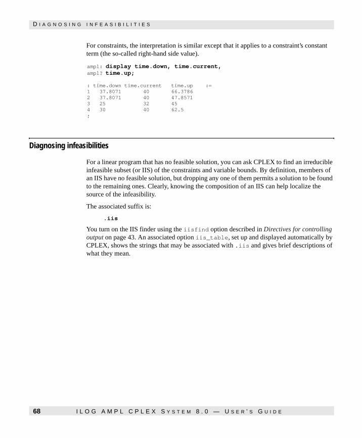
D I A G N O S I N G I N F E A S I B I L I T I E S
For constraints, the interpretation is similar except that it applies to a constraint’s constant term (the so-called right-hand side value).
Diagnosing infeasibilities
For a linear program that has no feasible solution, you can ask CPLEX to find an irreducible infeasible subset (or IIS) of the constraints and variable bounds. By definition, members of an IIS have no feasible solution, but dropping any one of them permits a solution to be found to the remaining ones. Clearly, knowing the composition of an IIS can help localize the source of the infeasibility.
The associated suffix is:
.iis
You turn on the IIS finder using the iisfind option described in Directives for controlling output on page 43. An associated option iis_table, set up and displayed automatically by CPLEX, shows the strings that may be associated with .iis and gives brief descriptions of what they mean.
ampl: display time.down, time.current,ampl? time.up;
: time.down time.current time.up :=1 37.8071 40 66.37862 37.8071 40 47.85713 25 32 454 30 40 62.5;
68 I L O G A M P L C P L E X S Y S T E M 8 . 0 — U S E R ’ S G U I D E

Defin
ed S
uffixes fo
r C
PL
EX
D I A G N O S I N G I N F E A S I B I L I T I E S
The following example shows how IIS finding might be applied to the infeasible diet problem from chapter 2 of the AMPL book. After solve detects that there is no feasible solution, it is repeated with the iisfind directive:
You can use display to look at the .iis values that have been returned:
This information indicates that the IIS consists of four lower and three upper bounds on the variables, plus the constraints providing the lower bound on B2 and the upper bound on NA in the diet. Together these restrictions have no feasible solution, but dropping any one of them will permit a solution to be found to the remaining ones. (Of course, in our example, we shouldn’t actually drop the lower bounds on the Buy variable - we could end up with negative values. However, we could reduce certain lower bounds to zero.)
ampl: model diet.mod;ampl: data diet2.dat;ampl: option solver cplexamp;ampl: solve;
CPLEX 8.0: infeasible problem7 iterations (7 in phase I)
ampl: option cplex_options ’iisfind 1’;ampl: solve;
CPLEX 8.0: iisfind 1CPLEX 8.0: infeasible problem0 iterations
Returning iis of 7 variables and 2 constraints.
suffix iis symbolic OUT;
option iis_table ’\0 non not in the iis\1 low at lower bound\2 fix fixed\3 upp at upper bound\’;
ampl: display _varname, _var.iis, _conname,ampl? _con.iis;: _varname _var.iis _conname con.iis:=1 "Buy[’BEEF’]" upp "diet[’A’]" non2 "Buy[’CHK’]" low "diet[’B1’]" non3 "Buy[’FISH’]" low "diet[’B2’]" low4 "Buy[’HAM’]" upp "diet[’C’]" non5 "Buy[’MCH’]" non "diet[’NA’]" upp6 "Buy[’MTL’]" upp "diet[’CAL’]" non7 "Buy[’SPG’]" low . .8 "Buy[’TUR’]" low . .;
I L O G A M P L C P L E X S Y S T E M 8 . 0 — U S E R ’ S G U I D E 69

D I R E C T I O N O F U N B O U N D E D N E S S
Direction of unboundedness
For an unbounded linear program—one that effectively has a minimum objective value of -Infinity or a maximum of +Infinity—the "solution" is characterized by a feasible point together with a direction of unboundedness from that point. On return from CPLEX, the values of the variables define the feasible point. The direction of unboundedness is given by an additional value associated with each variable through the associated solver-defined suffix:
.unbdd
An application of the direction of unboundedness can be found in our example of Benders decomposition applied to a transportation-location problem. One part of the decomposition scheme is a subproblem obtained by fixing the variables Build[i], which indicate the warehouses that are to be built, to trial values build[i].
When all values build[i] are set to zero, no warehouses are built, and the primal subproblem is infeasible. As a result, the dual formulation of the subproblem - which always has a feasible solution - is unbounded. When this dual problem is solved from the AMPL command line, CPLEX returns the direction of unboundedness in the expected way:
ampl: model trnloc1d.mod;ampl: data trnloc1.dat;ampl: problem Sub: Supply_Price, Demand_Price,ampl? Dual_Ship_Cost, Dual_Ship;ampl: let {i in ORIG} build[i] := 0;ampl: option solver cplexamp;ampl: option cplex_options ’presolve 0’;ampl: solve;
CPLEX 8.0: presolve 0CPLEX 8.0: unbounded problem30 iterations (0 in phase I)variable.unbdd returned
suffix unbdd OUT;
70 I L O G A M P L C P L E X S Y S T E M 8 . 0 — U S E R ’ S G U I D E

Defin
ed S
uffixes fo
r C
PL
EX
D I R E C T I O N O F U N B O U N D E D N E S S
The suffix message indicates that .unbdd has been created automatically. You can use this suffix to display the direction of unboundedness, which is quite simple in this case:
ampl: display Supply_Price.unbdd;
Supply_Price.unbdd [*] := 1 -1 6 -1 11 -1 16 -1 21 -1 2 -1 7 -1 12 -1 17 -1 22 -1 3 -1 8 -1 13 -1 18 -1 23 -1 4 -1 9 -1 14 -1 19 -1 24 -1 5 -1 10 -1 15 -1 20 -1 25 -1;ampl: display Demand_Price.unbdd;
Demand_Price.unbdd [*] :=A3 1 A6 1 A8 1 A9 1 B2 1 B4 1;
I L O G A M P L C P L E X S Y S T E M 8 . 0 — U S E R ’ S G U I D E 71

D I R E C T I O N O F U N B O U N D E D N E S S
72 I L O G A M P L C P L E X S Y S T E M 8 . 0 — U S E R ’ S G U I D E

C H A P T E R
CP
LE
X statu
s cod
es in
AM
PL
9
CPLEX status codes in AMPL
Solve codes
When CPLEX returns control to AMPL after a solve command, built-in AMPL parameters and an AMPL option provide information on the outcome of the optimization, as shown:
ampl: model oil.mod;ampl: data oil.dat;ampl: option solver cplexamp;ampl: display solve_result_num, solve_result;
solve_result_num = -1solve_result = ’?’
ampl: solve;
CPLEX 8.0: optimal solution; objective 12.2083432437 iterations (0 in phase I)
ampl: display solve_result_num, solve_result;
solve_result_num = 0solve_result = solved
ampl: option solve_result_table;
option solve_result_table ’\0 solved\100 solved?\200 infeasible\300 unbounded\400 limit\500 failure\’;
I L O G A M P L C P L E X S Y S T E M 8 . 0 — U S E R ’ S G U I D E 73

S O L V E C O D E S
The session log shows that the built-in AMPL parameter solve_result_num is -1 initially and parameter solve_result is ’?’. The solve invocation resets these parameters, however, so that they describe CPLEX's status at the end of its run—the solve_result_num parameter by a numeric code and solve_result by a message string. In the example shown, solve_result_num is set to 0 and solve_result to solved, indicating normal termination.
The AMPL option solve_result_table lists the valid combinations of solve_result_num and solve_result, for CPLEX. These combinations should be interpreted as shown below.
Status ranges are normally used to control algorithmic flow in AMPL scripts, where solve_result_num can be tested to distinguish among cases that must be handled in different ways. It is occasionally useful, however, to make fine distinctions among different solver termination conditions. All valid solve codes, with the corresponding termination message from CPLEX, are listed in the table below.
Table 9.1 Interpretation of numeric result codes
Number String Interpretation
0 – 99 solved optimal solution found
100 – 199 solved? optimal solution indicated, but error likely
200 – 299 infeasible constraints cannot be satisfied
300 – 399 unbounded objective can be improved without limit
400 – 499 limit stopped by a limit (such as on iterations)
500 – 599 failure stopped due to solver error
Table 9.2 Solve codes and termination messages
Number Message at termination
0 optimal solution
1 primal has unbounded optimal face
2 optimal integer solution
3 optimal integer solution within mipgap or absmipgap
100 best solution found, primal-dual feasible
200 infeasible problem
201 infeasible with phase II singularities
74 I L O G A M P L C P L E X S Y S T E M 8 . 0 — U S E R ’ S G U I D E

CP
LE
X statu
s cod
es in
AM
PL
S O L V E C O D E S
202 infeasible with phase I singularities
203 optimal with unscaled infeasibilities
204 converged, dual feasible, primal infeasible
205 converged, primal and dual infeasible
206 best solution found, primal infeasible
207 best solution found, primal-dual infeasible
208 infeasible or unbounded in presolve
220 integer infeasible
300 unbounded problem
301 converged, primal feasible, dual infeasible
302 best solution found, dual infeasible
400 phase II objective limit exceeded
401 phase II iteration limit
402 phase I iteration limit
403 phase II time limit
404 phase I time limit
405 primal objective limit reached
406 dual objective limit reached
410 node limit with no integer solution
411 time limit with no integer solution
412 treememory limit with no integer solution
420 mixed integer solutions limit
421 node limit with integer solution
422 time limit with integer solution
423 treememory limit with integer solution
Table 9.2 Solve codes and termination messages (Continued)
Number Message at termination
I L O G A M P L C P L E X S Y S T E M 8 . 0 — U S E R ’ S G U I D E 75
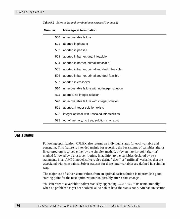
B A S I S S T A T U S
Basis status
Following optimization, CPLEX also returns an individual status for each variable and constraint. This feature is intended mainly for reporting the basis status of variables after a linear program is solved either by the simplex method, or by an interior-point (barrier) method followed by a crossover routine. In addition to the variables declared by var statements in an AMPL model, solvers also define "slack" or "artificial" variables that are associated with constraints. Solver statuses for these latter variables are defined in a similar way.
The major use of solver status values from an optimal basic solution is to provide a good starting point for the next optimization run, possibly after a data change.
You can refer to a variable’s solver status by appending .sstatus to its name. Initially, when no problem has yet been solved, all variables have the status none. After an invocation
500 unrecoverable failure
501 aborted in phase II
502 aborted in phase I
503 aborted in barrier, dual infeasible
504 aborted in barrier, primal infeasible
505 aborted in barrier, primal and dual infeasible
506 aborted in barrier, primal and dual feasible
507 aborted in crossover
510 unrecoverable failure with no integer solution
511 aborted, no integer solution
520 unrecoverable failure with integer solution
521 aborted, integer solution exists
522 integer optimal with unscaled infeasibilities
523 out of memory, no tree; solution may exist
Table 9.2 Solve codes and termination messages (Continued)
Number Message at termination
76 I L O G A M P L C P L E X S Y S T E M 8 . 0 — U S E R ’ S G U I D E

CP
LE
X statu
s cod
es in
AM
PL
B A S I S S T A T U S
of a simplex solver, the same display lists the statuses of the variables at the optimal basic solution. For example, consider the following:
A table of the recognized CPLEX status values is stored in the AMPL option sstatus_table displayed above. Numbers and short strings representing status values are given in the first two columns. The numbers are mainly for communication between AMPL and CPLEX, though you can access them by using the suffix .sstatus_num in place of .sstatus. The entries in the third column are comments.
The output of the display command shows that variable InCr[’MID_C’] is in the basis and InCr[’W_TEX’] at its lower bound at optimality.
You can change a variable’s basis status using AMPL’s let command. This may be useful in instances where you want to provide an initial basis to jump-start CPLEX.
ampl: model oil.mod;ampl: data oil.dat;ampl: option solver cplex;ampl: solve;
CPLEX 8.0: optimal solution; objective 12.2083432437 iterations (0 in phase I)
ampl: option sstatus_table;
option sstatus_table ’\0 none no status assigned\1 bas basic\2 sup superbasic\3 low nonbasic <= (normally =) lower bound\4 upp nonbasic >= (normally =) upper bound\5 equ nonbasic at equal lower and upper bounds\6 btw nonbasic between bounds\’;
ampl: display InCr.sstatus;
InCr.sstatus [*] :=MID_C basW_TEX low;
I L O G A M P L C P L E X S Y S T E M 8 . 0 — U S E R ’ S G U I D E 77

B A S I S S T A T U S
78 I L O G A M P L C P L E X S Y S T E M 8 . 0 — U S E R ’ S G U I D E

A P P E N D I X
A
CPLEX Synonyms
The following list contains alternative names for certain CPLEX directives. The use of primary names is recommended.
Synonym Primary Directive
agglim aggfill
dense densecol
display lpdisplay
doperturb perturb
endbasis writebasis
endvector writevector
growth bargrowth
heuristic rootheuristic
iterations lpiterlim
mipsolutions solutionlim
nodes nodelim
I L O G A M P L C P L E X S Y S T E M 8 . 0 — U S E R ’ S G U I D E 79

nodesel nodeselect
presolvedual predual
startalg mipstartalg
startalgorithm mipstartalg
startbasis readbasis
startvector readvector
subalgorithm mipalgorithm
time timelimit
treememory treememlim
varsel varselect
writeprob file
Synonym Primary Directive
80 I L O G A M P L C P L E X S Y S T E M 8 . 0 — U S E R ’ S G U I D E

I N D E X
Index
$ symbolnotation for options 12
.bestnodesuffix 66
.currentsuffix 67
.directionsuffix 65
.downsuffix 67
.iissuffix 68
.prioritysuffix 65
.unbddsuffix 70
.upsuffix 67
:= syntaxset initial values 13
A
absmipgapdirective 56
advancedirective 34
aggcutlimdirective 47
aggfill
directive 32aggregate
directive 32algorithm
directives for selection 30mixed integer 45
algorithmic controldirectives 50
AMPL$ notation for options 12batch mode 8command line switches 19configuration table 2description 1end session 7execute solver outside AMPL 16installing 2launching AMPL 7learning the AMPL language 2let command 77licensing 4requirements 2solver interface 11
ampl: prompt 7append directives 27ASCII format
problem and solution files 14autoopt
directive 31auxiliary files
I L O G A M P L C P L E X S Y S T E M 8 . 0 — U S E R ’ S G U I D E 81

I N D E X
creating 15
B
backtrackdirective 51
baralgdirective 38
barcorrdirective 38
bardisplaydirective 43
bargrowthdirective 38
bariterlimdirective 41
barobjrangedirective 38
baroptdirective 31
baroutofcoredirective 38
barrier algorithmdirectives 38
barstartdirective 39
barthreadsdirective 39
barvarupdirective 39
basic solutionsimplex algorithm 29
basissimplex algorithm 29
basisintervaldirective 34
batch mode 8bbinterval
directive 51bestnode
suffix 66binary format
problem and solution files 14boundstr
directive 47
branchdirective 52
C
cliquecutsdirective 47
clocktypedirective 41, 57
coeffreducedirective 48
commandlet 77option 12, 19option solver 11predefined commands 20solution 14write 14, 15
command line switches 19commands
display 13comptol
directive 39concurrentopt
directive 31configuration 2covercuts
directive 47CPLEX
append directives 27barrier algorithm 23barrier algorithm QP extension 25choice of algorithm 29cplex_options option 26linear programs 29memory requirement for linear programs 30mixed integer algorithm 45optimization methods 29problems handled by CPLEX 23specifying CPLEX directives 25
crashdirective 35
crossoverdirective 39
current
82 I L O G A M P L C P L E X S Y S T E M 8 . 0 — U S E R ’ S G U I D E

I N D E X
suffix 67cutpass
directive 48cuts
generate 47polyhedral 47
cutsfactordirective 48
D
densecoldirective 39
dependencydirective 33
dgradientdirective 36
directionsuffix 65
directiveabsmipgap 56advance 34aggcutlim 47aggfill 32aggregate 32autoopt 31backtrack 51baralg 38barcorr 38bardisplay 43bargrowth 38bariterlim 41barobjrange 38baropt 31baroutofcore 38barstart 39barthreads 39barvarup 39basisinterval 34bbinterval 51boundstr 47branch 52cliquecuts 47clocktype 41, 57coeffreduce 48
comptol 39concurrentopt 31covercuts 47crash 35crossover 39cutpass 48cutsfactor 48densecol 39dependency 33dgradient 36disjcuts 47doperturb 40dual 30dualopt 31dualthresh 30endtree 57feasibility 40file 43flowcuts 47flowpathcuts 47fraccand 48fraccuts 47fracpass 48gubcuts 47heuristicfreq 52iisfind 43impliedcuts 47integrality 56logfile 43lowercutoff 56lowerobj 41lpdisplay 43lpiterlim 41markowitz 40maximize 32minimize 32mipalgorithm 52mipcrossover 52mipcuts 47mipdisplay 60mipemphasis 52mipgap 56mipinterval 60mipstartstatus 49mipstartvalue 49
I L O G A M P L C P L E X S Y S T E M 8 . 0 — U S E R ’ S G U I D E 83

I N D E X
mipthreads 53mircuts 47netfind 37netopt 31nodefile 53nodelim 59nodeselect 51objdifference 57optimality 40ordering 39ordertype 54pdswitch 36perturbation 40perturblimit 40pgradient 35plconpri 54plobjpri 54precompress 33predual 33prereduce 33prerelax 49presolve 33presolvenode 49prestats 34pricing 37primal 30primalopt 31priorities 59probe 49readbasis 42readvector 42refactor 37relax 32relobjdiff 57round 54scale 34sensitivity 44siftopt 31simthreads 37singular 42solutionlim 59sos1 49sos2 50startalgorithm 55starttree 57
strongcand 55strongit 55strongthreads 55timelimit 42, 59timing 44, 60treememlim 59uppercutoff 56upperobj 41varselect 55version 44workfiledir 38, 53workfilelim 38, 53writebasis 42writevector 42xxxstart 37
directivesalgorithmic control 50append additional CPLEX directives 27control barrier algorithm 38control output 43, 60control simplex algorithm 34CPLEX directives 25CPLEX directives for linear programs 30halt and resume search 57improving stability 40preprocessing 32preprocessing, integer programs only 47relax optimality 56select algorithm 30starting and stopping 41store multiple 26
disjcutsdirective 47
display command 13doperturb
directive 40down
suffix 67dual
directive 30dual simplex algorithm 29dualopt
directive 31dualthresh
directive 30
84 I L O G A M P L C P L E X S Y S T E M 8 . 0 — U S E R ’ S G U I D E

I N D E X
E
editingusing a text editor 7
end AMPL session 7endtree
directive 57
F
feasibilitydirective 40
filecreating auxiliary 15predefined commands 20
filedirective 43
filesload several files 9temporary directory 17
flowcutsdirective 47
flowpathcutsdirective 47
fraccanddirective 48
fraccutsdirective 47
fracpassdirective 48
G
gubcutsdirective 47
H
heuristicfreqdirective 52
I
iissuffix 68
iisfinddirective 43
impliedcutsdirective 47
installation 2Unix 3Windows 3
integer programs 23integrality
directive 56
L
launching AMPL 7licensing 4linear programs 23
CPLEX solution method 29logfile
directive 43lowercutoff
directive 56lowerobj
directive 41lpdisplay
directive 43lpiterlim
directive 41
M
markowitzdirective 40
Markowitz threshold 41Markowitz tolerance 41maximize
directive 32memory
requirement for linear programs 30running out 60
memory usageexecute solver outside AMPL 16
messagestermination 74
minimizedirective 32
I L O G A M P L C P L E X S Y S T E M 8 . 0 — U S E R ’ S G U I D E 85

I N D E X
MIPdifficult subproblems 62
mip_prioritiesoption 52
mipalgorithmdirective 52
mipcrossoverdirective 52
mipcutsdirective 47
mipdisplaydirective 60
mipemphasisdirective 52
mipgapdirective 56
mipintervaldirective 60
mipstartstatusdirective 49
mipstartvaluedirective 49
mipthreadsdirective 53
mircutsdirective 47
N
netfinddirective 37
netoptdirective 31
network primal simplex algorithm 29nodefile
directive 53nodelim
directive 59nodeselect
directive 51nonlinear quadratic programs 23numeric result codes
interpretation 74
O
objdifferencedirective 57
optimalitydirectives for relaxing 56
optimalitydirective 40
optimizationmethods available in CPLEX 29
optioncautions 19eexit 19funcwarn 20gentimes 20linelim 20mip_priorities 52outopt 20presolve 20randseed 20substout 20times 20version 20
optionsadd options 12persistent settings 20preserve settings 21set options 19specify solver options 12
orderingdirective 39
ordertypedirective 54
out of memory 16output
directives for controlling 60directives for controlling output 43
P
pdswitchdirective 36
persistent option settings 20perturbation
directive 40
86 I L O G A M P L C P L E X S Y S T E M 8 . 0 — U S E R ’ S G U I D E

I N D E X
perturblimitdirective 40
pgradientdirective 35
piecewise linear programstransformation 24
plconpridirective 54
plobjpridirective 54
precompressdirective 33
predualdirective 33
preprocessingdirectives 32directives, integer programs only 47
prereducedirective 33
prerelaxdirective 49
presolvedirective 33
presolvenodedirective 49
prestatsdirective 34
pricingdirective 37
primaldirective 30
primal simplex algorithm 29primal-dual barrier algorithm 29primalopt
directive 31priorities
directive 59priority
suffix 65probe
directive 49problem file
ASCII format 14binary format 14
problem files 13
Q
quadratic programming 24
R
RAMrequirement for linear programs 30
readbasisdirective 42
readvectordirective 42
refactordirective 37
relaxoptimality 56
relaxdirective 32
relobjdiffdirective 57
requirementsAMPL 2
rounddirective 54
S
save output 14saving temporary files 14scale
directive 34search
directives for stopping and starting 57sensitivity
directive 44siftopt
directive 31simplex algorithm
basic solution 29directives 34
simthreadsdirective 37
singulardirective 42
solution
I L O G A M P L C P L E X S Y S T E M 8 . 0 — U S E R ’ S G U I D E 87

I N D E X
display information 13save output 14saving a solution 14
solution command 14solution file
ASCII format 14binary format 14
solution files 13solutionlim
directive 59solve codes 73, 74solver
add solver options 12choosing 11display solution information 13execute outside AMPL 16interface 11multiline options 12options 12problem files 13set initial values 13solution files 13specify options 12use of initial values 13
sos1directive 49
sos2directive 50
stabilitydirectives for improving 40
startalgorithmdirective 55
startingdirectives 41
starttreedirective 57
stoppingdirectives 41
strongcanddirective 55
strongitdirective 55
strongthreadsdirective 55
suffix
.bestnode 66
.current 67
.direction 65
.down 67
.iis 68
.priority 65
.unbdd 70
.up 67switches
-Cn 19command line 19-en 19-f 20-L 20-ostr 20-P 20-S 20-s 20-sn 20-T 20-t 20-v 20
T
temporary filesdirectory 17saving 14
termination messages 74text editor
using 7text file
predefined commands 20time
to find solution 44to read problem 44to write solution 44
timelimitdirective 42, 59
timingdirective 44, 60
treememlimdirective 59
troubleshootingcommon difficulties 60
88 I L O G A M P L C P L E X S Y S T E M 8 . 0 — U S E R ’ S G U I D E

I N D E X
U
unbddsuffix 70
Unix installation 3up
suffix 67uppercutoff
directive 56upperobj
directive 41usage notes 4
V
varselectdirective 55
versiondirective 44
W
Windows installation 3workfiledir
directive 38, 53workfilelim
directive 38, 53write command 14, 15writebasis
directive 42writevector
directive 42
X
xxxstartdirective 37
I L O G A M P L C P L E X S Y S T E M 8 . 0 — U S E R ’ S G U I D E 89

I N D E X
90 I L O G A M P L C P L E X S Y S T E M 8 . 0 — U S E R ’ S G U I D E