
iii - Aaltolib.tkk.fi/Diss/2001/isbn9512254611/isbn9512254611.pdf · 3.2.7 Model errors ... 5...
243
Transcript of iii - Aaltolib.tkk.fi/Diss/2001/isbn9512254611/isbn9512254611.pdf · 3.2.7 Model errors ... 5...


iii
ACKNOWLEDGEMENTS
The research presented in this dissertation was carried out at the Mechanical
Process and Recycling Laboratory, Department of Materials Science and Rock
Engineering, Helsinki University of Technology (HUT). Concrete castings were
performed at the concrete laboratory of Fortum Technologies in Vantaa and the statistical
modelling was carried out at the Laboratory of Computational Engineering, Department
of Electrical and Communications Engineering, Helsinki University of Technology. The
work was financed by Lohja Rudus Oy Ab, and the initiation for the dissertation was
introduced by the Scancem Scientific Counsel.
I would profoundly like to thank Professor Kari Heiskanen, under whose
supervision this study was carried out. The technical support was never compromised
whenever that was needed.
I also wish to thank Professor Göran Fagerlund and Dr Ernst M∅ rtsell for
reviewing the dissertation and for their comments and suggestions on the text.
Additionally, I want to extend my gratitude to Professor Jouko Lampinen for reviewing
the statistical approach of the dissertation.
The support of my employer, Lohja Rudus Oy Ab is gratefully acknowledged and
especially the encouragement received from M.Sc. Martti Kärkkäinen and M.Sc. Kauko
Linna is highly appreciated.
I want to express my sincere gratitude to M.Sc. Ville Toivanen for diligent and
intelligent assisting work, Mr. Tuomo Rimpiläinen and his group at Fortum for
accurately performed concrete castings and M.Sc. Aki Vehtari for the demanding
statistical modelling. Also the work of Mr. Ilkka Kalliomäki for the statistical program is
gratefully appreciated. It has been truly enjoyable and easy to work with all of you.
Many thanks are due to my colleagues at Lohja Rudus Oy Ab and the Laboratory
of Mechanical Process and Recycle for their support and interest as well as for
interdisciplinary and witty discussions.
Special thanks are due to my friends close by and abroad for balancing the life.
Finally, I wish to thank my parents for everything.
Hanna Järvenpää

iv
CONTENTS
Abstract ii
Acknowledgements iii
Contents iv
Definitions and notations xi
1. Introduction 1
2. Effects of aggregate characteristics on concrete properties 42.1 Workability 4
2.1.1 Effect of paste and water content 42.1.2 Effect of aggregate grading, surface area and size 52.1.3 Effect of aggregate shape, angularity and surface texture 62.1.4 Effect of aggregate mineralogy 72.1.5 Effect of aggregate absorption 82.1.6 Effect of superplasticizer and air-entraining agent 10
2.2 Air percentage 112.2.1 Air-void formation and stability 112.2.2 Effect of water-cement ratio 122.2.3 Effect of aggregate grading 122.2.4 Effect of aggregate shape, angularity and surface texture 132.2.5 Effect of aggregate mineralogy 142.2.6 Effect of superplasticizer 14
2.3 Bleeding 142.3.1 Definition of stability, viscosity and cohesion 142.3.2 Effect of cement and workability 152.3.3 Effect of aggregate surface area, grading and size 152.3.4 Effect of aggregate shape, angularity and surface texture 162.3.5 Effect of superplasticizer and air-entraining agent 17

v
2.4 Compressive strength 172.4.1 Effect of water-cement ratio and
aggregate-paste interface 172.4.2 Effect of compaction degree 192.4.3 Effect of aggregate size 192.4.4 Effect of aggregate strength 202.4.5 Effect of aggregate shape, angularity and surface texture 202.4.6 Effect of aggregate surface area 222.4.7 Effect of aggregate mineralogy 222.4.8 Effect of superplasticizer and air-entraining agent 23
2.5 Drying shrinkage 242.5.1 Mechanism of drying shrinkage 242.5.2 Effect of water-cement ratio 242.5.3 Effect of aggregate content 252.5.4 Effect of elastic modulus of aggregate 252.5.5 Effect of aggregate grading, shape, size, angularity
and surface texture 252.5.6 Effect of aggregate shrinkage properties 262.5.7 Effect of superplasticizer and air-entraining agent 27
3. Data analysis – methods and Excel –program used 283.1 Inputs – outputs 283.2 Bayesian statistics and Gaussian processes for prediction of
the fine aggregate-concrete interaction 293.2.1 Bayesian methods 293.2.2 Gaussian Process 293.2.3 Relevance values of inputs 323.2.4 Deviance Information Criterion (DIC) for model evaluation 333.2.5 Data pre-processing 343.2.6 Model selection 343.2.7 Model errors (prediction errors) 35

vi
3.3 Excel program for prediction of fine aggregate – concrete interaction 353.3.1 General principles of the Excel program 353.3.2 Predicting the correlation in input variables 363.3.3 Sensitivity analysis and its reliability 37
3.4 Error estimation 39
4. Experimental programme 404.1 Materials 40
4.1.1 Aggregate products 404.1.2 Cement 414.1.3 Admixtures 42
4.2 Test programme 434.2.1 Aggregate (inputs) 434.2.2 Concrete (outputs) 44
4.3 Mix designs and concrete mixes, mixing procedure, test specimens 464.3.1 Mix designs and concrete mixes 464.3.2 Mixing procedure 494.3.3 Test specimens 50
4.4 Testing methods and potential input values, aggregates 514.4.1 Mineralogical composition, fines and semi-coarse fractions 514.4.2 Specific surface area, fines 514.4.3 Grading, fines 554.4.4 Particle density, fines and semi-coarse factions 554.4.5 Particle porosity, fines and semi-coarse fractions 564.4.6 Zeta potential, fines 574.4.7 Resistance to fragmentation, semi-coarse fractions 584.4.8 Elongation, flakiness, particle volume and quantity,
semi-coarse fractions 584.4.9 Angularity/roundness, semi-coarse fractions 604.4.10 Surface texture, semi-coarse fractions 61

vii
4.5 Testing methods and concrete output values 624.5.1 Workability 624.5.2 Air % and density of fresh concrete 634.5.3 Bleeding 644.5.4 Compressive strength and density of the hardened concrete 64
4.6 Testing methods for drying shrinkage, weight loss and air-parameters,hardened concrete 664.6.1 Drying shrinkage and weight loss 664.6.2 Thin section analysis; air %, specific surface area and
spacing factor of air void 67
5 Aggregate test results and discussion 685.1 Mineralogical composition 695.2 Grading 705.3 Specific surface area 745.4 Particle density 765.5 Particle porosity 785.6 Zeta potential 835.7 Resistance to fragmentation 855.8 Elongation, flakiness, particle volume and quantity 865.9 Angularity and surface texture 905.10 Discussion of the test results for aggregates 93
6. Concrete test results and discussion 966.1 Workability 966.2 Air % 101
6.2.1 Air %, fresh concrete 1016.2.2 Air %, hardened concrete 105
6.3 Bleeding 1076.4 Compressive strength 1106.5 Drying shrinkage and weight change 114
6.5.1 Results 1146.5.2 Discussion 118

viii
7. Models for the fine aggregate – concrete interaction 1207.1 Model for the flow value 120
7.1.1 Sensitivity analysis – flow value 1227.1.1.1 Reliability of the sensitivity analysis – flow value 1227.1.1.2 Flow value – SC-flakiness 3.15/4.0 mm, SC-angularity and
SC-elongation 3.15/4.0 mm 1227.1.1.3 Flow value – SC-pore area 300-900Å and
SC- pore area >900Å 1247.1.1.4 Flow value – F- mica %, F- Cu, F- BET value and
F-zeta potential 125
7.2 Model for air %, fresh concrete 1287.2.1 Sensitivity analysis – air % 129
7.2.1.1 Reliability of the sensitivity analysis – air % 1297.2.1.2 Air % - SC-pore area 60-300Å and SC-pore area 300-900Å 1307.2.1.3 Air % - SC- flakiness 3.15/4.0 mm and SC-angularity 1317.2.1.4 Air % - F- Cu and F- BET value 133
7.3 Model for the bleeding 1347.3.1 Sensitivity analysis – bleeding 135
7.3.1.1 Reliability of the sensitivity analysis – bleeding 1357.3.1.2 Bleeding – SC- total pore area and SC- average pore area 1367.3.1.3 Bleeding – SC- elongation 0.8/1.0 mm,
SC- flakiness 1.6/2.0 mm and SC- elongation 1.6/2.0 mm 1377.3.1.4 Bleeding – F- BET value, F- zeta potential,
F- density and Cu 139
7.4 Model for the compressive strength 1427.4.1 Sensitivity analysis – compressive strength 144
7.4.1.1 Reliability of the sensitivity analysis –compressive strength 144
7.4.1.2 Compressive strength – SC- flakiness 3.15/4.0 mm andSC- quantity 1.6/2.0 mm 144
7.4.1.3 Compressive strength – SC- Los Angeles value 1457.4.1.4 Compressive strength – SC- pore area 60-300Å 145
7.5 Discussion of the models 147

ix
8. Predicting with the models 1508.1 Principles of the predictions 150
8.1.1 Combined effect of two input characteristics 1508.1.2 Predictions with different solutions for concrete
aggregate combination 151
8.2 Predicting with the flow value model 1538.2.1 SC- pore area 300-900Å and SC- flakiness 3.15/4.0 mm
vs. flow value 1538.2.2 F- Cu and SC- flakiness 3.15/4.0 mm vs. flow value 1568.2.3 Effect of different aggregate combinations on the flow value 159
8.3 Predicting with the air % model 1608.3.1 SC- pore area 60-300Å and SC- flakiness 3.15/4.0 mm vs. air % 1608.3.2 SC- pore area 60-300Å and F- Cu vs. air % 1618.3.3 Effect of different aggregate combinations on the air % 163
8.4 Predicting with the bleeding –model 1648.4.1 SC- total pore area and F- BET value vs. bleeding 1648.4.2 SC- total pore area and SC- elongation 0.8/1.0 mm vs. bleeding 1658.4.3 Effect of different aggregate combinations on the bleeding 167
8.5 Predicting with the compressive strength model 1688.5.1 SC- Los Angeles value and SC- flakiness 3.15/4.0 mm vs.
compressive strength 1688.5.2 SC- Los Angeles value and SC- pore area 60-300Å vs.
compressive strength 1718.5.3 Effect of different aggregate combinations on
the compressive strength 174
8.6 Discussion of the predictions made with the models 175
9. Verification of the models with two new aggregtate products 1799.1 Procedure 1799.2 Identification of the new aggregate products 1799.3 Results of the modelled and measured values 1809.4 Evaluation of the verification of the modelled and measured values 183

x
10. Conclusion 184
11. Need for future research 188
REFERENCES 189

xi
DEFINITIONS AND NOTATIONS
Aggregate
Granular material used in construction. Aggregate may be natural, manufactured or
recycled.
Natural aggregate
Aggregate from mineral sources which has been subjected to nothing more than
mechanical processing.
Natural fine aggregate
Designation given to smaller aggregate sizes with upper nominal size less than or equal
to 4 mm. Fine aggregate can be produced from natural disintegration of rock or gravel
and/or by the crushing of rock or gravel.
Fines
Particle size fraction of an aggregate, which passes the 0.063 mm sieve (aggregate
testing) or the 0.125 mm sieve (concrete castings).
AE air-entrainment (concrete)
ARD Automatic Relevance Determination
DIC Deviance Information Criterion
F fines (< 0.063 mm or 0.125 mm see above)
FG future gravel
GP Gaussian Process
gSH good shape
gST good strength (Los Angeles value)
MCMC Markov Chain Monte Carlo
N no admixture (concrete)
PG past gravel
pSH poor shape
pST poor strength (Los Angeles value)
SC semi-coarse
SCF semi-coarse fraction (0.125 – 4 mm)
WR superplasticizer (concrete)

1
1. Introduction
For the aggregate producer, the concrete aggregates are end products, while, for the
concrete manufacturer, the aggregates are raw materials to be used for mix designs and
successful concrete production. With the aggregate production, the quality of the
aggregate products can be influenced, but the raw material – the gravel or rock - may
have characteristics which cannot be modified by the production process. Similarly, with
the concrete mix designs can be influenced how the aggregate affects the properties of
concrete, but there is also a limit, whether technical and/or economic, in the mix design
modification after which it is useful to select a more suitable aggregate product.
Concrete aggregates have been studied relative largely in the past decades, though most
of the research has been done to the coarse aggregate and only to one or few quality
characteristics at a time. In order to optimise the aggregate-concrete chain, one has to
know what are the aggregate quality characteristics that dominate different concrete
properties, and how basic changes in the concrete mix design affect the influences. The
need for knowledge is increasing as conventional concrete aggregate supplies are
becoming depleted, and environmental aspects prevent the use of existing sources.
The objectives of this work are:
1. To determine which the most important fine aggregate characteristics are that
affect the concrete workability, compressive strength, air %, bleeding and drying
shrinkage.
2. To determine how the aggregate characteristics affect the concrete properties
separately and together.
3. To determine how basic changes in the concrete mix design, i.e. change in paste
amount and admixtures (air-entraining agent, superplasticizer) affect the
aggregate influences.
4. To become a program with which can be predicted how the fine aggregate –
concrete interaction affects the concrete workability, compressive strength, air %
and bleeding.

2
When the objectives are fulfilled, the results are applicable for optimising both the
aggregate and concrete production.
The experimental studies were divided to aggregate tests for aggregate characteristics
determination and to concrete tests where the tested aggregates were used for concrete
production and observation of behaviour in concrete properties. To be able to relate the
extent that the aggregate has on the concrete as compared against the effect of the
changes in mix design, the test programme was built to monitor the aggregate behaviour
in different mix designs including variations in admixtures and paste amount. The test
programme was additionally constructed in such a way that the effect of the fines and the
semi-coarse fraction could be interpreted separately. The fines are defined in this study as
the fractions bellow 125 µm and the semi-coarse fractions as particle sizes between 125
µm and 4 mm. The aggregate characteristics and basic concrete mix design changes are
regarded as input variables and the fresh and hardened concrete properties are the
outputs to be modelled.
Due to the restricted amount of data and lack of knowledge concerning which aggregate
characteristics are relevant and their relationships to the concrete properties, it was
decided to apply the Bayesian statistics and non-parametric non-linear Gaussian process
models. The Bayesian statistics is based on learning processes where the prior
information is combined with the evidence from the data. The results are treated as
probability distributions expressing our beliefs regarding how likely the different
predictions are. In a non-parametric model, the aggregate characteristics – concrete
properties relationship is determined from the data without reference to an explicitly
parameterised model and thus, the possible different behaviour of aggregate inputs in the
different mix design conditions can be concurred in the model. The adoption of a non-
linear model enables the possibility of non-linear conduct of the aggregate
characteristics.
The statistical modelling was performed by the laboratory of computational engineering
at the Technical University of Helsinki.

3
The results of the models in this study are presented in the following formats:
1. ARD (Automatic Relevance Determination) listing gives the relevance values of the
inputs, i.e. aggregate characteristics and basic mix design changes, in each model.
The relevance value determines the distance of each input in the space of the model
over which the input is expected to vary significantly.
2. Sensitivity analysis figures present how the output changes when an input variable is
changed by a small amount. The predicted output is calculated and by comparing the
change made in the input variable to the change perceived in the output, we see how
the model reacts to changes in that particular input variable. The sensitivity analysis
figures are presented for all inputs in each of the models except for SEM/N/AE/WR
which are of nature “on/off”.
3. Sensitivity reliability figures present the difference between the modelled and
measured values and thus, indicate how reliable the model is in general and on
specific input-output-mix design combination.
4. Example predictions of combined effect of two aggregate input characteristics
present how the models can be used for predictions for the combined effect on one
output of two input characteristics over their total variation range. The result is
shown by means of 3D surface charts and in the calculations the other characteristics
of the model have fixed values. The charts are drawn for each mix design separately,
as the mix design parameters (SEM, N/AE/WR) are additional influencing
characteristics for the output. The example predictions are executed to one possible
future solution for concrete aggregate combination.
5. Example predictions with different solutions for concrete aggregate combination
present how the models can be used for predicting the effect of different aggregate
products on the concrete properties. The results are shown in column charts and for
each mix design separately, as the mix design parameters (SEM(N/AE/WR) are
additional influencing characteristics for the outputs. In these predictions all the input
characteristics are changed according to the aggregate combination. The example
predictions are executed to three different solutions for concrete aggregate
combinations; past and future gravel and combination of filler aggregate and crushed
rock including predictions for the variation on shape and strength characteristics.
6. Verification of the models with two new aggregate products.

4
2 EFFECTS OF AGGREGTE CHARCTERISTICS ON CONCRETE
POPERTIES
2.1 Workability
2.1.1 Effect of paste and water content
Any mix made with given materials and having a certain consistency will have a point at
which the water ratio or the voids ratio is at a minimum. This point of maximum solids
content also determines the optimum paste consistency. POWERS (1968) has defined the
optimum paste consistency as follows: “Optimum paste consistency is that consistency at
which the solids content of the paste and the paste content of the mix are such that they
produce the maximum solids content possible with the given materials.”. Several
commercial programs for particle packing prediction are now available, e.g. LPDM
(Linear Packing Density Model) and Europack.
For the concrete mix to be plastic, the volume of the cement paste must be sufficient to
fill the interstitial space of the compacted aggregate, plus an increment that causes a
certain dispersion of the aggregate particles (figure 1). (POWERS 1968, KRONLÖF 1997)
Figure 1. Dry compacted state of the aggregate skeleton (A)
Aggregate particles dispersed in cement paste (B) (POWERS 1968)

5
In plastic mixes, it is not paste alone that causes the dispersion of aggregate particles and
plasticity; the volume of the paste is always augmented by a certain amount of air.
According to the excess paste theory, the consistency of concrete depends on two factors:
the volume of cement paste in excess of the amount required to fill the voids of the
compacted aggregate; and the consistency of the paste itself. If the aggregate/cement
ratio or the cement content of the mix for given materials is kept constant, the
workability is then governed by the water amount. (POWERS 1968)
MØRTSELL (1996) proposed functions for workability prediction of mortars and concrete.
The inputs of the functions are the flow resistance ratio ( Qλ ) which characterises the
matrix phase and the air voids space modulus ( mH ) which characterises the aggregate
phase. For a given matrix and aggregate phase, the volume relations between the phases
determine the workability of the mortar or concrete. The matrix phase consists of water,
cement, pozzolanes, admixtures and filler (<0.125 mm aggregate).
2.1.2 Effect of aggregate grading, surface area and size
When the grading is changed for given materials, then the surface area of the aggregate
combination is also affected. The greater the exposed surface area is the more water and
cement paste will be required to wet that area and, therefore, the less water and paste will
remain to lubricate the mix and thus the lower its workability will be. Special mix
proportioning methods based on the specific surface of the aggregate combination have
been proposed by, e.g. SINGH (1959). In his method the specific surface is determined by
the water permeability method or an estimation is made on the basis of a shape factor.
The specific surface of a combination of spheres of fine aggregate, fS , is given by:
���
����
� +++++=32168421100
654321 ppppppSS f Equation 1
where

6
S = the specific surface of the smallest size group,
i.e. No. 100/ No. 200 sieves (0.075/0.150 mm)
61...pp = percentage weight of six groups in the fine aggregate,
from the smallest to the largest (0.075-0.150-0.300-0.600-1.2-2.4-4.8 mm)
LOUDON (1952-53) studied the shapes of different fine aggregates and he arrived at a
determination of angularity factor, f, where the angularity is expressed as the ratio of the
specific surface of a size group to the specific surface of spheres of a corresponding size
group. He suggested that f = 1.1 for a rounded fine aggregate, f = 1.25 for a fine
aggregate of medium angularity, and f = 1.4 for an angular fine aggregate. The specific
surface is thus shape corrected by multiplying the specific surface of spheres by an
appropriate angularity factor.
MURDOCK (1960) suggested a modified method that also takes the maximum particle size
into account. In addition to having a relatively smaller surface area requiring wetting an
increased maximum aggregate size also presents the possibility of denser packing.
With a given quantity of paste, decreasing the percentage of fine aggregate decreases the
surface area, and hence the surface tension, thus tending to increase the mobility of the
mix. In lean mixes (those with a low amount of cement) and gap graded mixes, the
percentage of fine aggregate should, however, be high enough to ensure sufficient
cohesion. Concrete mixes of which good mobility is required should also have an
adequate surface area enabling good cohesion and shear resistance (see 2.2).
2.1.3 Effect of aggregate shape, angularity and surface texture
As was discussed earlier, the shape factors influence the specific surface; aggregates
which are flaky, elongated and/or angular thus require more paste to wet the surfaces.
The shape and texture of the aggregate also affect the bulk density of the aggregate
skeleton and for rough, poor-shaped aggregate, the bulk density is therefore less than that
of smooth, well-rounded particles of the same density owing to particle friction and

7
interference. Filling the voids and overcoming the friction call for a higher content of
fine aggregate and water. A higher cement amount may also be necessary, to keep the
strength constant.
When a mix becomes richer, the angularity and grading of the aggregates become less
important until, with high proportions of cement, the aggregate particles are little other
than “plums” floating in cement paste. The test results obtained by MURDOCK (1960)
show that, when the aggregate/cement ratio is reduced to 2, the effects of angularity and
grading become negligible.
KAPLAN (1958) studied 13 different coarse aggregates and came to the conclusion that
increased angularity and/or flakiness lead to a reduction in the workability of concrete.
Changes in the angularity, however, have a greater effect on the workability of concrete
than changes in the flakiness. In Kaplan’s studies flakiness caused 20% of the variation
in the workability, whilst 59% was due to angularity. Although in his study there was a
wide variation in the surface texture of the aggregates, Kaplan did not find any
correlation between aggregate surface texture and the workability of concrete.
In his research WILLIS (1967 studied nine different fine and coarse aggregates. He found
that an equal change in shape characteristics caused fine aggregate to need two to three
times more water than coarse aggregates. He also noted that the shape characteristics
described the concrete behaviour best, whereas the mortar tests also included the effects
of clay, mica and other deleterious materials. Owing to the method that was used to
determine the shape (flow rate through an orifice), we can conclude that the findings
reported by Willis are actually caused by a combination of shape, angularity and surface
texture effects.
2.1.4 Effect of aggregate mineralogy
Clay minerals are normally sheet-shaped i.e. they have more surface area than other
minerals of the same grain size. The ratio of thickness to length for clay particles is

8
normally near 20. This makes the surface area of a clay particle nearly three times that of
a cube of the same volume (non-expanding clays).
Clays normally have a charged surface, and thus they attract charged ions and/or water
molecules to adsorb on the surface. With some clays, the activity of the surface is
increased by a sort of internal surface into which charged ions and water molecules can
find their way (expanding clays). These absorbed ions and molecules expand the clay,
and the surface area can be increased by a factor of 25 or more. (VELDE 1995)
DANIELSEN AND RUESLÅTTEN (1984) studied micas in the size range of 0.15/0.30 mm.
They found that micas have a negative effect on the workability properties of concrete.
The effect is even greater for muscovite than for biotite, but only in the case of newly
crushed, unweathered micas. For gravel-based, weathered micas, there is no difference
in behaviour between muscovite and biotite.
Particle degradation during mixing (flaky and elongated or otherwise mechanically weak
particles) may cause an increased water requirement, slump loss, and a reduced air
content of the air-entrained concrete. Additionally, if the aggregate particles have a
coating which is soft or loosely adherent, the coating may be removed during the mixing
and this would increase the fines amount of the grading.
2.1.5 Effect of aggregate absorption
The mix design procedure now prevailing in Finland is based on the total water/cement
ratio, i.e. the aggregate is considered to be in the bone-dry state. The mix design
procedure most commonly applied in other countries is based on the effective
water/cement ratio, which excludes the water absorbed by the aggregates (figure 2). This
is also the case with EN 206-1, “Concrete – Part 1: Specification, performance,
production and conformity”.

9
Figure 2. Different aggregate moisture conditions (NEVILLE 1995)
The effective water/cement ratio and the free water content are difficult to determine. For
both coarse and fine aggregates, the absorption of bone-dry aggregate to the state of
saturated and surface dry (SSD) is determined with standard tests that are hence accurate,
though both methods have their own reproducibility and repeatability errors. Normally, it
is assumed that, at the time of the setting of concrete, the aggregate is in an SSD
condition. When aggregates are dry, e.g. in spring and summer the particles may quickly
get coated with cement paste which prevents the further ingress of water necessary for
saturation; in consequence, the effective water/cement ratio is higher than assumed. On
the other hand, when the water/cement ratio is calculated on the bone-dry basis, the
effective water content is always less than calculated recipe water. In this case, too, the
effective water content varies according to the prevailing moisture content of the
aggregate products and mix designs, as in richer mixes the coating effect of the cement
tends to be quicker than in leaner mixes. (SINGH 1958, NEVILLE 1995)
Most of the water absorption occurs by the outer layer of the aggregate particles. Some
aggregates, especially gravel products, can have a weathered “patina” outer layer. The
minerals of the outer surface can be altered and/or some minerals may have been leached
away, causing enhanced porosity. The weathered gravel with a “patina” outer layer
absorbs more than crushed product produced from the same raw material. This is due to
the fresh, less porous unweathered surfaces, which appear during crushing. (KAPLAN
1958)

10
2.1.6 Effect of superplasticizer and air-entraining agent
When an air-entraining admixture is used the water content and/or the share of fine
aggregate can be reduced. An 1 per cent increase in air is equivalent to a 1 per cent
increase in fine aggregate or a 3 per cent increase in the unit water content (ACI
COMMITTEE 309, 1981). The reason for the improved workability brought about by the
entrained air is that the air bubbles, kept spherical by surface tension, act as a fine
aggregate having a very low surface friction and considerable elasticity. Figure 3 shows
the indicative reduction of the water content as a function of the percentage of added air
and the cement content.
Figure 3. Reduction in the mixing water due to entrained air (NRCA 1993)
For very lean mixes with an aggregate/cement ratio of 8 or more, and particularly when
an angular aggregate is used, the improvement in workability caused by air entrainment
is such that the resultant decrease in the water/cement ratio compensates fully for the loss
of strength resulting from the presence of the voids. (POWERS 1968)
Superplasticizers adsorb onto the surface of cement and aggregate particles and alter the
electrical charge of the surface and/or cause physical interference (steric repulsion)
between particles. The deflocculation and dispersion of cement and aggregate fines is
thus enhanced and the workability is increased.

11
2.2 Air percentage
2.2.1 Air-void formation and stability
Entrapped air voids are unintentional voids. They are characteristically 1000 microns or
more in diameter and, because the periphery of the voids follows the contour of the
surrounding aggregate particles, they are usually irregular in shape. Entrained air voids,
in the contrast, are spherical or nearly so, owing to the hydrostatic pressure to which they
are subjected by the surrounding paste of water, cement and aggregate fines. These voids
are typically between 10 and 1000 microns in diameter. (MIELENZ ET AL. 1958)
Air-entraining agents adsorb at air-water interfaces, and thus the air voids that are formed
during mixing become stabilised as they are covered by a sheath of air-entraining
molecules that repel one another. Repellence prevents the coalescence of voids and
ensures uniform dispersion of the entrained air. The soluble air-entraining agents will
also precipitate on the surface of cement and aggregate particles, and will reduce the
hydrophilic quality of the surface and render it hydrophobic. Air voids tend to cling to
the hydrophobic surface of the particles. It is thus anticipated that void-particle adhesion
is most significant for certain ranges of particle size. Studies of ore flotation indicate that
particles between about 10 and 50 microns in sizes are most susceptible to void adhesion.
(NEVILLE 1995, MIELENZ ET AL. 1958)
Often there is a discrepancy between the air content measured in fresh concrete and air
content determined in hardened concrete. Three mechanisms have been proposed for air-
void instability in fresh concrete (FAGERLUND 1990):
1. Loss of coarse air voids due to handling and compaction as the large bubbles
move upwards by buoyancy
2. Dissolution of small bubbles in water as the bubbles collapse due to pressure
caused by surface tension
3. Transfer of air from small bubbles to coarse bubbles as small bubbles coalescence
with larger bubbles

12
2.2.2 Effect of water-cement ratio
The amount of entrained air is smaller with lower water/cement ratios, i.e. with higher
cement concentrations. WHITING (1985) has reported that dosages as much as ten times
greater are needed for 6.5 ±1.0% entrainment for concrete with a w/c of 0.30..0.32 (SSD)
and a maximum aggregate size of 25 mm as compared against dosages used in
conventional concrete mixes. The same phenomenon can be seen in figure 4, the air
entrainment in cement paste where is presented for different w/c ratios and air-
entrainment agent dosages. (POWERS 1968)
Figure 4. Air entrainment in cement paste as influenced by the w/c ratio and the
dosage of air-entraining agent (POWERS 1968)
2.2.3 Effect of aggregate grading
The air content of concrete increases if the proportion of intermediate size (150 – 600
µm) of fine aggregate is increased. The maximum size of the space subtended by
intermediate particles varies from about 30 to 130 microns. The size range is suitable for
enmeshing air-entrained bubbles that are big enough to withstand rapid dissolution in the
mixing water. An increase in the finer sizes of aggregate or cement beyond the optimum

13
intermediate size decreases the air content because the available volume among the
particles is decreased and hence the air bubbles become smaller. The smaller bubbles are
subjected to greater pressure than bigger bubbles, thus increasing the dissolution of the
bubbles. Further, an increase in coarse aggregate size decreases the available interstitial
space of optimum dimensions and thus decreases the air content in concrete. (MIELENZ
ET AL. 1958, SINGH 1959, PIGEON AND PLEAU 1995)
2.2.4 Effect of aggregate shape, angularity and surface texture
When the shape and/or angularity of the aggregate particles deviates from sphericity, the
interstitial space between the particles decreases if the most compact arrangement of the
particles is achieved. If good workability is required, the paste content of the mix design
is increased, which enlarges the interstitial space and leads to successful air entrainment
(NICHOLS JR. 1982, MIELENZ 1958). On the basis of his tests, SINGH (1959) concluded
that angular particles derive great benefit for purposeful air entrainment as they resist
compaction and thus increase the interstitial space between particles.
BACKSTROM ET AL. (1958) studied eleven aggregates, including aggregates with smooth
and rough surfaces. They found that surface texture had a to be rather striking effect on
the values of the specific surface and spacing factor in air-entrained castings. The
average value of the surface area was 742 in-1 for the smooth aggregates and 1037 in-1 for
the rough aggregates. The average values of the spacing factor were 0.0065 and 0.0045
in., respectively. They found a fairly good correlation between the spacing factor and the
freezing and thawing resistance with seven out of the eleven aggregates they tested. Four
concrete castings expanded more than would have been expected according to the
spacing factor. These aggregates all had smooth surfaces, and in petrographic
examination they were found to contain appreciable amounts of weathered and physically
unsound materials.

14
2.2.5 Effect of aggregate mineralogy
The effect of aggregates on the air-entrainment agent function varies according to the
chemical and mineralogic compositions and degrees of alteration (see 2.5.4). Aggregates
composed with alkali earth and metallic ions, e.g. limestone, dolomite, blast furnace
slags and glassy basalts, are expected to have the most considerable effect on the
performance of the air-entraining agent. (MIELENZ 1958)
2.2.6 Effect of superplasticizer
If superplasticizers are used to increase the workability of concrete, the air content of air-
entrained concrete generally increases if the other mix design parameters are constant. In
some cases, however, the air is not stable, i.e. the air-void system created during the
concrete manufacturing changes before the concrete is hardened. This has been explained
by two phenomena (PLANTE ET AL. 1989):
1. superplasticizers can entrain large bubbles, which are thus easily lost during
handling and compaction
2. superplasticizers increase the paste fluidity, thereby promoting the coalescence of
air-voids.
2.3 Bleeding
2.3.1 Definition of stability, viscosity and cohesion
Stability is defined as the flow of fresh concrete without applied force and is measured by
bleeding and segregation characteristics. Bleeding occurs when the mortar is unstable
and releases free water. Normal bleeding, which occurs in the form of uniform seepage,
is not necessarily undesirable. It is, e.g. good preventive curing against plastic shrinkage
cracking. Segregation is defined as the instability of a mix, caused by a weak matrix that

15
cannot retain individual aggregate particles in a homogeneous dispersion. Segregation is
possible in the case of both wet and dry consistencies.
Viscosity is defined as the quotient of shear stress divided by the rate of shear in a steady
flow. The viscosity of the matrix can also be said to contribute to the ease with which the
aggregate particles can move and rearrange themselves within the mix.
Cohesion is defined as the force of adhesion between the matrix and the aggregate
particles. It provides the tensile strength of fresh concrete that resists segregation.
Internal friction occurs when a mix is displaced and the aggregate particles translate and
rotate. (ACI COMMITTEE 309, 1981)
2.3.2 Effect of cement and workability
The fineness and the amount of cement greatly affect the bleeding tendency of concrete.
Finer cement decreases this tendency owing to its larger surface area, earlier hydration
and lower sedimentation rate. In addition, less bleeding occurs when cement has a high
alkali and C3A content. (NEVILLE, 1995)
A water content above that needed to achieve a workable mix produces greater fluidity
and decreased friction. Additionally, the water-cement ratio increases; this reduces the
cohesion within the mix and hence increases the potential for segregation and excessive
bleeding. An overly dry mix may also result in loss of cohesion and dry segregation. (ACI
COMMITTEE 309, 1981)
2.3.3 Effect of aggregate surface area, grading and size
The amount and surface area of the fine aggregate, especially that smaller than 150 µm,
influences the bleeding of the concrete. The increased bleeding caused by the angularity
of the fine aggregate can be controlled by the surface area. The bleeding tendency is

16
reduced by using a finer fine aggregate or by adding separate fines to the mix. The fines
automatically contained in the crushed fine aggregate as a result of the crushing
phenomenon is also suitable, though care should be taken that the amount is not too
much.
Mixes with gap grading normally require less water to achieve good workability than
continuous grading with an otherwise similar recipe. Gap grading reduces the sizes of
coarse fine aggregate and small coarse aggregate, and the tendency for bleeding and even
segregation is enhanced if the concrete has a high workability without enough cohesion
(cement, fines or air %). Additionally, if the fine aggregate fraction becomes coarse, the
cohesion is reduced thus making the mix harsh and the tendency for bleeding increases.
In contrast, as the fine aggregate becomes finer, the water requirement increases and the
concrete mix becomes increasingly sticky.
If the coarse aggregate has a large maximum size and if, in addition, the particles are
flaky an excessively workable concrete should be avoided because pockets of bleed
water may collect on the undersize of the coarse aggregate particles.
2.3.4 Effect of aggregate shape, angularity and surface texture
Flakiness, elongation, angularity and surface texture of the aggregate, especially with the
fine aggregate, all reduce the workability of concrete. The viscosity of the paste increases
if only water is added, and if the surface area of the paste (cement, additives, fines and
air) is too low, the extra water can overcome the cohesion and vigorous bleeding or even
segregation can occur.

17
2.3.5 Effect of superplasticizer and air-entraining agent
Superplasticizers generally reduce bleeding except if there is a very high slump when the
concrete can become unstable and heavy bleeding or even segregation can occur.
(NEVILLE 1995)
Air entrainment also reduces bleeding. The reduction is caused by the displacement of
the paste, the buoyancy of the bubbles and their surface area. (POWERS 1968)
2.4 Compressive strength
2.4.1 Effect of the water-cement ratio and aggregate-paste interface
Concrete is a heterogeneous material. Its properties depend on the properties of its
component phases and the interactions between them. If concrete is fully compacted, the
compressive strength for a given set of materials at a given age is inversely proportional
to the water/cement ratio. It has been observed, however, if the water/cementitious
material ratio and the fine aggregate/cement ratio of the concrete and mortar are constant,
the cement paste has the highest compressive strength and ductility compared to mortar
and concrete. Additionally, mortar has a somewhat higher compressive strength and a
little more ductility than concrete, but otherwise possesses a similar stress-strain curve,
figure 5.(MARTIN ET AL. 1991)
According to DARWIN (1999) the lower strength of mortar and concrete results from
stress concentrations induced in the cement paste by the aggregate particles. The stress
peaks are due to differences in the elastic properties of aggregate and paste. Failure of the
paste-aggregate interface also plays a role here, but generally to a lesser degree.

18
Figure 5. Stress-strain curves for concrete, mortar and cement paste with
a water/cementitious material ratio of 0.5 (MARTIN ET AL. 1991)
The weakness of the aggregate-matrix interface may be explained by the following
phenomena:
a) development of a higher porosity than the bulk matrix (higher w/c ratio)
b) formation of larger crystal particles of the hydration products
c) deposition of calcium hydroxide crystals with a preferential orientation on the
interface
MONTEIRO, MASO AND OLLIVIER (1985) found that the thickness of the transition phase
is determined by the intensity of the surface effects produced by the aggregate. The
thickness is larger for larger aggregates, and it is also a function of the size and shape of
the fine aggregate particles. The surface effects originated by the fine aggregate particles
interfere with those caused by the large aggregate, and the intensity of this interference
determines the final thickness of the transition zone. PING et al. (1991) discovered,
however, that for very fine limestone particles (radius ≤ 0.199 mm) the transition zone
was denser than bulk paste. They concluded this to be due to chemical reactions between
limestone particles and portland cement.

19
2.4.2 Effect of compaction degree
If the compaction of concrete is insufficient, the compressive strength is reduced.
KAPLAN (1960) observed, for example, that the compressive strength of concrete with a
voids content of 15% was reduced by approximately 72% when compared against the
strength of fully consolidated concrete This result was irrespective of the mix proportions
or the age at which the test was done. However, the reduction in strength due to a rise in
voids up to a content of 15 % was much greater than that, owing to an increase from 15%
up to 30%. The reduction percentage in concrete having a voids content of 30% was
found to be 92%. WALKER AND BLOEM (1959) concluded that, at a given water/cement
ratio the compressive strength of concrete containing up to about 10% entrained air, is
reduced by approximately 5% for every 1% of air added. Their conclusion agrees fairly
well with the results of KAPLAN (1960).
WRIGHT (1953) concluded that the effect on compressive strength is materially the same,
irrespective of whether the air is entrained intentionally in the form of numerous minute
bubbles or occurs unintentionally in the from of large irregular voids.
2.4.3 Effect of aggregate size
WALKER AND BLOEM (1960) have shown that, at a fixed water/cement ratio, strength
decreases as the maximum size of aggregate increases, particularly for sizes larger than
38 mm (1½ in.). The optimum size tends to decrease with increasing strength. This
phenomenon is caused by many parameters related to the heterogeneity of concrete, e.g.
the interface zone, lower bond stresses between the aggregate particles and the matrix,
maximum paste thickness and different dimensional changes of the paste and aggregate
at both early and later age (ALEXANDER ET AL. 1961, LALLARD AND BELLOC 1997).
However, reduction in the maximum aggregate size increases the specific surface of the
aggregates and thus the incidentally entrapped air tends to be higher or if the workability
is kept constant, the w/c ratio becomes higher. Both cases have a decreasing effect on the
compressive strength, unless the workability is controlled with superplasticizer.

20
2.4.4 Effect of aggregate strength
Most normal-weight aggregates have strengths much greater than the strength of the
cement paste. Thus, up to concrete strengths of about 35 to 40 MPa, the effects of
different good-quality aggregates are usually small. However, the aggregate strength
required is considerably higher than the normal range of concrete strengths, because the
actual stresses at the interface of individual particles within the concrete may be far in
excess of the nominal compressive stress that is applied.
In higher strength classes, the aggregate strength properties - which are also a function of
particle shape - as well as the bond between the paste and aggregate begin to play a more
important role. As the concrete is a heterogeneous material, the best compressive strength
results are achieved with aggregate, which has a high strength (e.g. a good Los Angeles
value) and low modulus of elasticity, i.e. a modulus of elasticity that is not very different
from hydrated cement paste. When the elasticity values are closer to each other, the bond
stresses are lower; thus less microcracking is induced and higher compressive strength
values can be achieved. For flexural strength, the compatibility of the modulus of
elasticity is even greater. (NEVILLE 1995)
2.4.5 Effect of aggregate shape, angularity and surface texture
WILLIS (1967) found that the shape of the fine aggregate had a markedly greater effect on
compressive strength than the coarse aggregate. Fine aggregate influenced the
compressive strength primarily through its effect on the need for mixing water, whereas
with coarse aggregate, other factors in addition to the water requirement affected the
compressive strength, e.g. elasticity, bond and mineralogy.
ALEXANDER (1959) concluded that if even slightly angular projections or depressions are
present on the surface of an otherwise smooth aggregate pebble, the mechanism of tensile
failure can change from a preferential rupture of the bond to a preferential rupture
through the paste in the region of the surface irregularity. (Figure 6. )

21
Figure 6. The rupture mechanism depends on the relationship between bond
and paste strengths as well as on the degree of irregularity on the surface
of the crushed aggregate particle. ALEXANDER (1959)
KAPLAN (1959) studied 13 different coarse aggregates and found, that the most important
factor in coarse aggregate affecting the compressive strength was the surface texture. A
rougher surface results in a greater adhesive force between the cement matrix and the
aggregate. In this study, the surface texture was determined by comparing the traced line
length from a magnification of 125 times against the length of an unevenness line drawn
as a series of chords.
One explanation for surface texture is the porosity of the particle surface. A porous, dry
surface absorbs water and thus positively influences the bond between the aggregate
particle and the paste. Additionally, if the aggregates are drier than SSD, the
water/cement ratio will be reduced by the absorption of the aggregates and, consequently,
the strength will increase. (STOCK ET AL. 1979, NEVILLE 1995)
When it comes to the effect of the shape, angularity and surface texture, it is somewhat
difficult to compare the results obtained by researchers, because nearly all the studies
have been conducted using different testing methods to determine the same
characteristics. Also, the terminology is overlapping to some extent, e.g. the line used to
distinguish between the surface texture and angularity is vague.
Aggregate
Paste
A C
B
B’A
B
C

22
2.4.6 Effect of aggregate surface area
STOCK ET AL. (1975) conducted tests to study the effect of the aggregate concentration
on the compressive strength of concrete. The results show that the strength of cement
paste in tension and in compression is reduced by the addition of 20% by volume of
graded aggregate, and it fell to a minimum value at a volume fraction of 30% to 35% and
then increased with a further addition of aggregate.
When the specific surface of aggregate is increased for a constant mix proportion, the
amount of cement relative to the surface of the aggregate decreases. LALLARD AND
BELLOC (1997) state that as the maximum paste thickness (MPT) between aggregate
particles decreases the compressive strength increases. In dry packing of particles, it has
been observed that the highest stresses exist at the contact points of aggregate particles.
Thus, when paste is introduced into the packing and it is placed between two close
aggregates, the paste will be highly stressed, yielding a greater matrix strength. The
results of GOBLE AND COHEN (1999) also showed that the mortar strength increased and
the strain-stress behaviour became more ductile as the quantity of the transition zone
material was increased, i.e. as the aggregate surface area was increased. They comment,
however, that increasing surface area causes stiffer mixtures, which is probably why in
the test series performed by SINGH (1958) it was noted that the increase in the aggregate
surface area caused more voids around the surface of the aggregate particles and thus a
decrease in compressive strength.
2.4.7 Effect of aggregate mineralogy
The mineral size, texture and mineralogical composition as well as the shape, angularity
and surface texture affect the strength properties of the aggregate products. Additionally,
the electrostatic conditions as well as the behaviour together with admixtures, additives
and cement depend on the mineralogy. Some chemical bond may exist between the

23
aggregate and cement paste in the case of limestone and dolomite aggregates and
possibly also siliceous aggregates. (NEVILLE 1995)
In their studies, DANIELSEN AND RUESLÅTTEN (1984) found that altered feldspars (An –
rich plagioclases) have an almost continuous transition zone from the mineral phase to
the cement paste phase. For unaltered feldspars, the contact zone was completely
discontinuous. They concluded that the altered feldspars, with their cation deficiency in
the crystal structure, make the diffusion of Ca from the cement paste into the Si-Al
framework possible. A similar phenomenon also occurs with mica minerals during
weathering. While unweathered mica (0.15/0.30 mm) caused a loss of strength in mortar,
mortar made with weathered mica didn’t deviate form the strength of the reference
mortar. Potassium leached during the weathering process helps the hydrated calcium ions
to find adsorption sites on the mica surfaces.
When mica is present in the coarse aggregate, the most important factor is not the total
amount of mica but its distribution. If the mica is in bundles, then even smaller amounts
of mica can be detrimental, though its effect can be also seen from the strength
determinations.
2.4.8 Effect of superplasticizer and air-entraining agent
Superplasticizers are used to increase the workability, to reduce the w/c ratio and/or to
save cement. Changes in the w/c ratio and cement amount have clear effects on
compressive strength. By reducing the water without compromising the workability, the
24-hour early strength can be increased by 50% to 75%. Owing to the better dispersion of
the cement particles, a greater amount of reactive surface area of cement is exposed,
which can also lead to increased compressive strength. (NEVILLE 1995)
The effect of entrained air has been discussed in chapter 2.4.2.

24
2.5 Drying shrinkage
2.5.1 Mechanism of drying shrinkage
Concrete holds water in various states with different bonding energies. These are
capillary water, which is free from the influence of surface forces, adsorbed water; which
is bound to a solid surface; and interlayer water, which penetrates between a pair of solid
surfaces. Drying shrinkage is observed as a result of the forces of contraction arising as
the water is removed by drying.
There are many models for determining the drying shrinkage of concrete. There is,
however, widespread agreement that the dominant factors are the modulus of elasticity of
the aggregate and cement paste (or their ratio), the aggregate content and, aggregate and
paste shrinkage. (PICKETT, 1956, HANSEN AND NIELSEN 1965, HANSEN AND
ALMUDAIHEEM 1987)
2.5.2 Effect of water-cement ratio
Shrinkage is greater the higher the water-cement ratio is, because the w/c ratio
determines the amount of evaporable water in the cement paste and, additionally, the rate
of evaporation. BROOKS (1989) concluded that the shrinkage depends on the
water/cement ratio up to a w/c ratio of approximately 0.6, after which the additional
water in the cement paste takes the form of free water. Unlike the physically (adsorbed)
and chemically (interlayer) bound water, the free water does not contribute to shrinkage.
Hence, the change in the volume of drying concrete is not equal to the volume of water
removed.

25
2.5.3 Effect of aggregate content
The aggregate in concrete restrains the drying shrinkage; this explains the higher
aggregate content the smaller shrinkage with a constant w/c ratio. According to the
model of HANSEN AND ALMUDAIHEEM (1987), the shrinkage decreases by about 18%
when the aggregate content is changed from 65% to 70%. This change is independent of
the w/c ratio, though the restraining effect of the aggregate is more pronounced with an
increasing w/c ratio. The effect of the aggregate content on concrete shrinkage has also
been reported by, e.g. PICKETT (1956).
2.5.4 Effect of elastic modulus of aggregate
The total restraining effect of aggregate depends not only on the volume concentration of
the particles but also on the elastic properties of the particles and paste. The modulus
ratio is defined as the ratio of the elastic modulus of the dispersed particles to the
hydration products. For normal-weight concrete, the modulus ratio is typically in the
range of 4 to 7. According to the model presented by HANSEN AND ALMUDAIHEEM
(1987), the difference in dying shrinkage of concrete having a volume of aggregate in the
range of 60% to 80% is about 30% when the modulus ratio increases from 4 to 7. When
the effect of same change in the modulus ratio is predicted with the model by presented
HANSEN AND NIELSEN (1965), the decrease in drying shrinkage is, however, only 8%.
The reason for this difference between the two models lies in the calculation of Young’s
modulus of elasticity, especially, how the aggregate effect is taken into account.
2.5.5 Effect of aggregate grading, shape, size, angularity and surface texture
The effect of aggregate grading, shape and size on concrete shrinkage is indirect and
depends on how these influence the amount of water amount in the concrete. On the
other hand, aggregate properties that enhance the bond between the paste and aggregate,

26
e.g. surface texture, angularity and porosity (see 2.3.6) decrease the drying shrinkage.
(ACI COMMITTEE 221, 1997)
2.5.6 Effect of aggregate shrinkage properties
Some aggregates are known to shrink on drying. In most cases, these aggregates also
have a high water absorption. Generally, aggregates containing quartz or feldspar and
granite, limestone, dolomite as well as some basalts can be classified as low-shrinkage
producing aggregates. Aggregates containing sandstone, shale, slate, graywacke, or some
types of basalt have been associated with high-shrinkage concrete. However, the
properties of a given aggregate type, such as granite, limestone or sandstone, can vary
considerably within different sources. This can result in significant variation in the
shrinkage of concrete made with a given type of aggregate. (ACI COMMITTEE 221, 1997)
In their studies, HANSEN AND NIELSEN (1965) concluded, that if any appreciable
shrinkage occurs in the aggregate material, the restraining effect of the particles is
reduced and that it is not usually possible to bring the concrete shrinkage within
reasonable limits by adjusting the composition of the concrete mix. Similar results were
reported previously by CARLSON (1939), as can be seen from table 1.
Table 1. Drying shrinkage of concrete with different aggregates (CARLSON 1939)
Aggregate
Particle density
[ Mg/m3 ]
Absorption
[ % ]
1-year drying shrinkage,
RH 50%
[ o/oo]
Sandstone 2.47 5.0 1.16
Slate 2.75 1.2 0.68
Granite 2.67 0.5 0.47
Limestone 2.74 0.2 0.41
Quartz 2.65 0.3 0.32

27
The presence of clay on the aggregate lowers its restraining effect on shrinkage.
Moreover, because the clay itself is subject to shrinkage, clay coatings can increase the
shrinkage by up to 70%. (POWERS 1959)
2.5.7 Effect of superplasticizer and air-entraining agent
If superplasticizer is used for water reduction then two opposite phenomena affect the
drying shrinkage. A lowered w/c ratio reduces the shrinkage, whereas the enhanced
dispersion of cement increases the effective surface area of the paste and thus increases
the shrinkage.
BROOKS (1989) studied five different plasticizers and superplasticizers in water reduced
and cement reduced concrete mixes and found that the admixtures increase the
deformation (shrinkage and creep) by 3% to 132% compared to plain concrete. His
suggestion was that for admixture flowing concrete (high workability), the deformation
expectation should be increased by 20%.
Entrainment of air has been found to have no effect on shrinkage. (KEENE 1960)

28
3. DATA ANALYSIS – METHODS AND EXCEL PROGRAM USED
3.1 Inputs – outputs
We studied how the fine aggregate characteristics affect the concrete properties. To be
able to relate the extent of the effect that the aggregate has on the concrete compared to
the effect of the mix design changes, the testing program was build to contain six
different mix designs in which 21 fine aggregate products were studied altogether in 215
castings. See section 4.
The fine aggregate characteristics and mix design parameters are input variables, and the
fresh and hardened concrete properties are the outputs to be modelled. (Figure 7)
Figure 7. Input – output scheme
These outputs have been modelled with the methods described in chapters 3.2 and 3.3.
The models can be used with the Excel –program described in chapter 3.4.
Additionally, concrete drying shrinkage and the air % in hardened concrete were studied,
but these were not modelled.
Mix design parameters
Fine aggregatecharacteristics
•Air %, fresh concrete•Flow value•Bleeding•Compressive strength
INPUTS OUTPUTS

29
3.2 Bayesian statistics and Gaussian processes for prediction of
the fine aggregate-concrete interaction
3.2. 1 Bayesian methods
Bayesian statistical methods use probability to quantify uncertainty in inferences. The
result of Bayesian learning is a probability distribution expressing our beliefs regarding
how likely the different predictions are. The prior information from the problem is
combined with the evidence from the data, giving the posterior probability of the
solutions. Predictions are made by integrating over this posterior distribution. The effect
of the prior information diminishes with increased evidence from the data and in the case
of insufficient data, the prior dominates in the solution. The article of GELMAN ET AL.
1995 gives a good introduction to Bayesian methods.
3.2.2 Gaussian Process
As it is not known what the parameterised form of the input-output relationship should
be, we use non-parametric non-linear Gaussian process (GP) models (RASMUSSEN 1996,
ABRAHAMSEN 1997, MACKAY 1998, NEAL 1997, NEAL 1999). In a nonparametric model,
the input-output relationship is determined from the data without reference to an
explicitly parameterised physical model. Gaussian processes are a natural way of
specifying prior distributions over possible relationships between the inputs and the
output. In material science, Gaussian Processes have been applied, e.g. to the problem of
predicting the microstructures of forged materials (BAILER-JONES ET AL. 1998) and the
austenite formation in steel (BAILER-JONES ET AL. 1999).
Based on the training data ( ) ( )( ) ( ) ( )( ){ }nn yxyxD ,,...,, 11= (having n data points), our
primary purpose is to predict the new output, ( )1+ny , for a new case where we have

30
observed only the new input vector, ( )1+nx . With Gaussian processes predictive
distribution of ( )1+ny is Gaussian, with the mean and variance given by
( )[ ] yCkDyE n 11 ´ −+ = Equation 2
( )[ ] kCkVDyVar n 11 ´ −+ −= Equation 3
where,
C is the n by n covariance matrix of the observed targets( ) ( ){ }nyyy ,...,1= is the vector of known values for these targets
k is the vector of covariances between ( )1+ny and the n known outputs
V is the prior variance of ( )1+ny (i.e. ( ) ( )[ ]11 , ++ nn yyCov ).
There are many possibilities for the covariance function, some of which are discussed in
(RASMUSSEN 1996, ABRAHAMSEN 1997, MACKAY 1998, NEAL 1999). For example, a
regression model based on a class of smooth functions can be obtained using a
covariance function of the form
( ) ( )( ) 2
1
222 exp σij
p
u
ju
iuuij dxxrsC +��
�
����
�−−= �
=Equation 4
The first term of this covariance function expresses that the cases with nearby inputs
should have highly correlated outputs. The s parameter gives the overall scale of the local
correlations. The ur parameters are multiplied by the co-ordinate wise distances in input
space and thus allow for different distance measures for each input dimension. For
irrelevant inputs, the corresponding ur should be small in order for the model to ignore
these inputs.
The second term is the noise model, where 1=ijd when i=j. For the noise model, we
tested normal and 4t distributions. The 4t distribution is Student's t distribution with 4
degrees of freedom, which is a quite safe and robust choice when the true noise
distribution is unknown.
It should be noted that this noise model is only for the outputs, and we assume here that
the inputs are noise-free. This assumption is wrong (we know there are measurement

31
errors in input variables), but we assume that this simplification still gives the model
acceptable accuracy. A noise model for the inputs would improve estimate of predictive
distribution and would allow reconstruction of the regression over the true noiseless input
– but such a noise model would be more complex to implement and to use. (CARROLL ET
AL. 1995, CORNFORD ET AL. 1998, WRIGHT 1999).
Our prior knowledge is usually insufficient to fix the appropriate values for the
hyperparameters in the covariance function (σ , s, and the ur for the model above).
Therefore the hyperparameters are given prior distributions and predictions are made by
integrating (averaging) over the posterior distribution for hyperparameters. This
integration can be done using Markov Chain Monte Carlo (MCMC) methods (GILKS ET
AL. 1996, GAMERMAN 1997, ROBERT & CASELLA 1999). In Monte Carlo methods
expectations of integrals are approximated by using a sample of values drawn from the
posterior distribution of parameters. In MCMC, samples are generated using a Markov
chain that has the desired posterior distribution as its equilibrium distribution.
We have used Flexible Bayesian Modeling (FBM) software (NEAL), which implements
the methods described in (NEAL 1996, NEAL 1997, NEAL 1999).
• The Gaussian process specification used was
gp-spec log nin 1 - - 0.01 / 0.05:0.5 0.05:0.5:1
• The noise model specification used was
model-spec log real 0.05:0.5:4
• The initial values for the model parameters were set as
gp-gen log fix 0.2 0.1
• The MCMC sampling parameters were set as
mc-spec log repeat 10 sample-variances heatbath 0.9 hybrid 10 0.15 negate
The length and the number of the chains and the burn-in length were decided using visual
inspection of trends and the potential scale reduction method (GELMAN AND RUBIN
1992A, GELMAN AND RUBIN 1992B).

32
3.2.3 Relevance values of inputs
In the GP model using a covariance function of the equation 4 the ur parameters are
sometimes called Automatic Relevance Determination (ARD) (GIBBS 1997, NEAL 1997,
NEAL 1999). The ARD parameter determines the distance to the particular direction in
the n-dimensional space (n = number of inputs) over which the data point is expected to
vary significantly, i.e. the ARD listing can be referred to as a listing of the relevance
values of the inputs.
We computed the relevance value for each input for each posterior sample of relevance
parameters ( ur ). This yields a sample from the posterior distribution of the relevance
values, which may be summarised to provide an estimate of the mean (asterisk) and
median (diamond) values for each input, plus 25%-75% (box) and 10%-90% (line)
quantiles. The quantiles describe the uncertainty of each input in relevance value. Figure
8 shows the relevance value listing of the inputs for the compressive strength 91 d model.
(See chapter 7.4.) Higher value describes a higher relevance for the specific input.
Figure 8. Example of a relevance value listing of inputs, compressive strength 91 d
Asterisk – mean value; diamond – median value;
box – 25-75 % quantiles; line - 10-90 % quantiles
WR
Flkn 3.15/4.0 mm
AE
Los Angeles
QNTY 1.6/2.0 mm
Pore area 10-300 Å
SEM
-4 -3 -2 -1 0 1

33
3.2.4 Deviance Information Criterion (DIC) for model evaluation
The purpose of interpolation problems is not usually to obtain the closest fit to the data
but to find a balance between fitting the data and making sensible predictions about new
events. Hugely complex models are often over-parameterised and, while fitting the data
precisely, they interpolate and extrapolate poorly. Within the classical modelling
framework, model comparison takes place by defining a measure of fit, typically the
deviance statistic, and complexity, the number of free parameters in the model. (GIBBS
1997, SPIEGELHALTER ET AL. 1998)
Deviance Information Criterion (DIC) was recently proposed by SPIEGELHALTER ET AL.
(1998) for comparison of arbitrarily complex Bayesian models.
DIC is based on comparison of the posterior distribution of the deviance
( ) ( ) ( )yfypD log2log2 +−= θθ ,
where y is the observed data and θ are the lowest-level parameters directly influencing
the fit. The standardising term ( )yf is a function of the data alone and hence does not
affect model comparison.
The fit of a model is summarised by the posterior expectation of the deviance
[ ]DED yθ= .
The model complexity is measured by the effective number of parameters Dp , defined as
[ ] [ ]( )θθθ yyD EDDEp −=
( )θDD −=

34
The fit and the complexity are then added to form a Deviance Information Criterion
DpDDIC +=
( ) DpD 2+= θ
The DIC and quantiles for it can be easily obtained from the MCMC analysis.
3.2.5 Data pre-processing
For computational reasons, input and output variables were normalised to have zero
mean and unit variance (BISHOP 1995 P.298, NEAL 1999). Some of the outputs (air %,
bleeding 60min) had values close to zero, but it is known that the values for these outputs
are always greater than zero. In order to assure that the predictions and predictive
quantiles for these outputs would always be greater than zero, log transformation was
used.
3.2.6 Model selection
First we made models with different noise models for each output with full set of
potential inputs (see chapter 4.4.). To compare different noise models, we calculated the
mean square error (MSE) and 90% quantiles of absolute error of the test data and
Bayesian Deviance Information Criterion (DIC). The 4t noise model was clearly better
than the Normal noise model for all outputs. Then, using relevance values of the inputs,
smaller sets of inputs were selected and new models were made (some inputs were
favoured over others, based on expert knowledge e.g. BET vs. pore area (fines); see
chapter 4.4.
We continued this approach for each output until the DIC increased. The best model
according to the DIC was selected and then, using backward selection, the input set was
still reduced. The model with the lowest DIC was selected. If several models had
statistically similar DIC values, the model with the least inputs was selected. Models

35
having the least inputs had similar errors compared to the errors of the model having all
inputs. Depending on which output was modelled, seven to twelve input variables were
needed. (see section 7.)
3.2.7 Model errors (prediction errors)
To estimate prediction errors we used a ten-fold cross-validation (10-CV) error estimate,
i.e. nine tenths of the data was used for training and the one tenth was left out for error
evaluation, and this scheme was repeated ten times (STONE 1974, GEISSER 1975,
GELFAND AND DEY 1994). All the castings were used for inferences, but error estimates
were computed only for castings with A and B aggregate products (no REF was used).
Quantiles of estimated prediction errors were obtained by re-sampling. Cross-validation
was used to produce cross-validation predictive densities (GELFAND 1996). Expectations
and quantiles were then easy to estimate by re-sampling MCMC samples and data points.
3.3 Excel program for prediction of fine aggregate – concrete interaction
3.3.1 General principles of the Excel program
When the desired input combination (fine aggregate characteristics and mix design
parameters) are entered into the Excel program, it will
• calculate the expectation value for the output and 10% and 90% quantiles for the
prediction (→ 3.3.2)
• suggest adjustments to other input variables when one variable is changed (→ 3.3.2)
• show how marginal changes of one input affect the specific output, i.e. it
demonstrates, the output sensitivity to an input variation (→ 3.3.3)
• show the reliability of the sensitivity analysis (→ 3.3.3).

36
3.3.2 Predicting the correlation in input variables
When a single input variable is changed by a large amount, we would like to take into
account the correlation between the inputs. All other inputs should be adjusted in such a
way that the new input vector is similar to those found in the training data set. This can
be done by calculating the covariance matrix of the data and adjusting the other inputs
according to the relative magnitude of the elements in the covariance matrix,
2
2
,,ii
ijiunchangedjchangedj dxxx
σσ
⋅+= . Equation 5
where
i is the index of the manually changed input
idx is the change made to that input
j is the index of the input to be adjusted
2ijσ is one element in the covariance matrix Σ
For practical purposes, it is better to use a regularised estimate for the covariance matrix.
This is done by Principal Component Analysis (PCA) (BISHOP 1995). First, the
maximum likelihood estimate for the covariance matrix is computed with
�=
−−=ΣN
i
Tii xxN 1
)()( ))((1 µµ ��
�
. Then, the eigenvectors iv and eigenvalues iλ of the
matrix Σ�
are computed, choosing M largest ones. The regularised estimate for the
covariance matrix is then TVVΛ=Σ~ , where the matrix Λ has M largest eigenvalues iλ
on the main diagonal and the matrix V contains corresponding eigenvectors iv as
columns. Using a regularised estimate has the advantage of making more conservative
adjustments to the inputs because less significant and noisy correlation effects are
ignored.

37
3.3.3 Sensitivity analysis and its reliability
Sensitivity analysis answers the question: “How does the output change when an input
changes?” At each data point, a single input variable is changed by a small amount (for
example, ±2%) and the predicted output is calculated. By comparing the change made in
the input variable to the change perceived in the output, we see how the model reacts to
changes in that particular input variable. A useful graph can be made by plotting the
input variable on the horizontal axis and connecting the predicted outputs of the original
and changed inputs with a line (Figure 9).
Figure 9. Example of an input-output sensitivity analysis
The slope of this line then represents the sensitivity of the model in one data point. If the
lines are horizontal, the change in the input variable has no effect on the output. Upward
and downward slopes suggest positive and negative effects in the output, respectively.
Having two data points with different slopes close to one another does not necessarily
mean that the model is incorrect; the change in the slope could be due to a large change
Sensitivity analysis
35
40
45
50
55
60
65
1.2 1.25 1.3 1.35 1.4 1.45
SC-Flkn 3.15/4.0 mm
Co
mp
. Ste
ng
th [
MP
a]
N30
WR30AE30N35WR35AE35

38
in other input variables, not illustrated in any way in the graph. The mutual correlation of
the input variables is ignored in this analysis, as the changes made in the inputs are small.
We would also like to estimate the reliability of our sensitivity analysis. By plotting the
input variable of interest on the horizontal axis and connecting the predicted and
measured output variables on the vertical axis with a line, we can identify ranges in the
input variable where prediction errors are large, and thus where the model is not to be
trusted (Figure 10).
Figure 10. Example of the reliability of a sensitivity analysis
In these areas, the results of the sensitivity analysis are likely to be incorrect as well. In
contrast, where the prediction errors are small, the results of the sensitivity analysis are
deemed to be more plausible.
Sensitivity analysis - difference between modelled and measured values
35
40
45
50
55
60
65
70
1.2 1.25 1.3 1.35 1.4 1.45
SC-Flkn 3.15/4.0 mm
Co
mp
. Ste
ng
th [
MP
a]
N30WR30AE30N35WR35AE35
39
3.4 Error estimation
For determining the error in output measurements, we repeated 15% of the castings.
From these repetitions we determined the repeatability error of measurement; it is the
median of the 90% quantile of the absolute error. It includes the error made by the
laboratory personnel as well as errors arising from differences in the conditions during
the repetitions. In addition, it includes the deviations within the raw materials between
the repetition castings. The skewness of the error prediction distribution can be observed
from the 10/50/90% quantiles of the 90% quantile of the absolute error. In the text is
used notation, e.g. “40 mm (30 – 60 mm)”, in which the 40 mm is the median (50%) of
the 90% quantile of the absolute error, and the values in parentheses give the 10% and
90% quantiles for the 90% quantile of the absolute error.
The model error includes the repeatability error of the measurement and the errors due to
the selected inputs and model. As discussed earlier, the model selection is normally done
by choosing the model where the fit and complexity are optimised. The input selection is,
of course, crucially important to the model performance. If the inputs aren’t capable of
describing the output phenomenon, then the lack of the fit of the model will be obvious
and hence the model error will be large. Also, the model error describes the median of
the 90% quantile of the absolute error and the notation in the text is similar to the
repeatability error notation.
The group average is the median of the 90% quantile for the mix design group results,
i.e. castings without admixture (N), with superplasticizer (WR) and with air-entraining
agent (AE). The largest group is that, where all the castings are included (all). When we
compare the group average to the repeatability error, we can evaluate the variation
caused by other factors, presumably that caused by the fine aggregate characteristics.

40
4 EXPERIMENTAL PROGRAMME
4.1 Materials
4.1.1 Aggregate products
Fine Aggregate products
A total twenty-one (21) different aggregate products were used in this study. Thirteen
(13) of these were gravel materials and eight (8) crushed rocks. Table 2 is presents the
aggregate products, their material source, rock type, used size fractions and geographical
origin.
Table 2. List of the aggregate products
Aggregate
Material
source Rock type
Used size fractions
fines / semi-coarse
Geographical
origin
A2 Rock Granite F & SC Uusimaa
A3 Rock Granite F & SC Uusimaa
A6 Rock Mica gneiss F Pohjois-Savo
A7 Rock Tonalite F & SC Uusimaa
A8 Rock Garnet bearing granite F & SC Pohjanmaa
A10 Rock Tonalite SC Pohjanmaa
A15 Rock Mafic metavolcanite F Pohjois-Savo
A16 Rock Gabbro F & SC Kanta-Häme
B1 Gravel Granitic gravel F & SC Uusimaa
B2 Gravel Granitic gravel F & SC Uusimaa
B3 Gravel Granitic gravel F Kymenlaakso
B6 Gravel Granitic gravel F Varsinais-Suomi
B7 Gravel Granitic gravel F & SC Pohjois-Savo
B8 Gravel Sandstone, granitic gravel F & SC Satakunta
B9 Gravel Sandstone F Satakunta
B10 Gravel Granitic gravel F Satakunta
B11 Gravel Granitic gravel F & SC Uusimaa
B12 Gravel Granitic gravel F & SC Päijät-Häme
B13 Gravel Granitic gravel F & SC Päijät-Häme
B14 Gravel Granitic gravel F & SC Uusimaa
REF Gravel Granitic gravel SC Uusimaa

41
Aggregate REF is the normal concrete laboratory aggregate used in Finland and was
chosen as a reference aggregate for this study.
More accurate mineralogical compositions of the aggregate products are presented in
tables 12 - 14 in chapter 5.
In order to control the mix design grading curve, the aggregate products were sieved to
six (6) nominal size fractions; 0/0.125, 0.125/0.25, 0.25/0.5, 0.5/1.0, 1.0/2.0 and 2.0/4.0
mm. Down to 0.25 mm the sieving was performed with a Mogen sieving apparatus, and
the two smallest size fractions were separated using a Sweco sieving machine. To ensure
accurate sieving results the size fractions 1.0/2.0 and 2.0/4.0 mm were sieved twice and
the size fractions 0.25/0.5 and 0.5/1.0 mm and 0/0.125 and 0.125/0.25 mm three times.
The REF aggregate was already sieved to narrow nominal size fractions; 0.1/0.6, 0.5/1.2,
1/2, 2/3 and 2/5 mm. Only the finest size fraction, 0.1/0.6 mm, was sieved using the
Sweco to obtain the fraction 0.125/0.6 mm. Appendix 1 presents the original gradings of
the aggregate products.
Coarse aggregate
The coarse aggregate was a combination of two coarse aggregate products. The nominal
sizes of the aggregate products were 5/10 and 8/14 mm. Both aggregate products were
uncrushed granitic gravels from Uusimaa.
4.1.2 Cement
The cement was Finnish rapid hardening cement, CEM IIA 42.5R. Table 3 presents its
chemical composition and physical characteristics. As it was already known from the
beginning that the total time for the castings would be long, extra care was taken to
prevent the cement from ageing. To verify the quality of the cement along the castings,
four (4) strength determinations were made. Table 4 shows the initial compressive
strength results and the three determinations done during the castings.

42
Table 3. Chemical composition and physical properties of cement
Chemical composition [ % ] Physical properties
CaO 61.3 Property Value
SiO2 19.6 Particle density 3.14 Mg/m3
Al2O3 4.8 Specific surface (Blaine) 473 m2/kg
MgO 3.0 Standard consistency 31.0 %
Fe2O3 2.4 Setting time, beginning 90 min
SO3 3.6 Setting time, end 150 min
Na2O eq 1.3
TiO2 0.3
Table 4. Compressive strength determinations
Age [ d ] Compressive strength [ MPa]
25.02.1998 25.08.1998 30.11.1998 08.02.1999
1 24.8 25.4 29.1 28.9
7 49.6 49.9 51.3 49.7
28 57.1 58.1 57.9 57.0
4.1.3 Admixtures
Two admixtures were used: a superplasticizer and an air-entrainment agent. The
superplasticizer was a sulphonated naphthalene formaldehyde condensate, Mighty 150. A
fatty acid soap-based product, Ilma-Parmix, was used as an air entrainment admixture.
The air entrainment agent was diluted to solution of 1:19. Both substances are
commercially available and commonly used admixtures in the concrete industry.
The dry material content for the water reducer is 42% and for the diluted air-entraining
agent 5%.

43
4.2 Test programme
4.2.1 Aggregate (inputs)
The test programme was divided into tests for the fines (F) and semi-coarse (SC) size
fractions separately partly because this is natural due to the magnitude difference
between them, but also in order to ascertain the effects of the characteristics in isolation
from each other. This is especially important with the processed fine aggregate products,
e.g. mixture of uncrushed gravel and rock products. For the purpose of better revealing
the variations in the characteristics, the fines were tested as the size fraction 0/0.063 mm.
Table 5 presents a list of the basic characteristics of the fine aggregate studied and the
test methods used. It also shows to which size fractions the tests have been applied.
Table 5. Basic characteristics of the fine aggregate studied and the test methods
used
Basic characteristic of the
fine aggregate Test method Tested size fraction(s)
Mineralogical composition Röntgen diffraction
(X –ray)
0/0.063 mm
2.0/4.0 mm
Specific surface area 1. BET-analysis
2. Laser diffraction 0/0.063 mm
Grading Laser diffraction 0/0.063 mm
Particle density Helium pycnometer 0/0.063 mm
2.0/4.0 mm
Particle porosity Mercury intrusion porosimetry 0/0.063 mm
0.5/1.0 mm
Zeta potential Zeta potential 0/0.063 mm
Resistance to fragmentation Los Angeles value, modified 4.0/5.6 mm
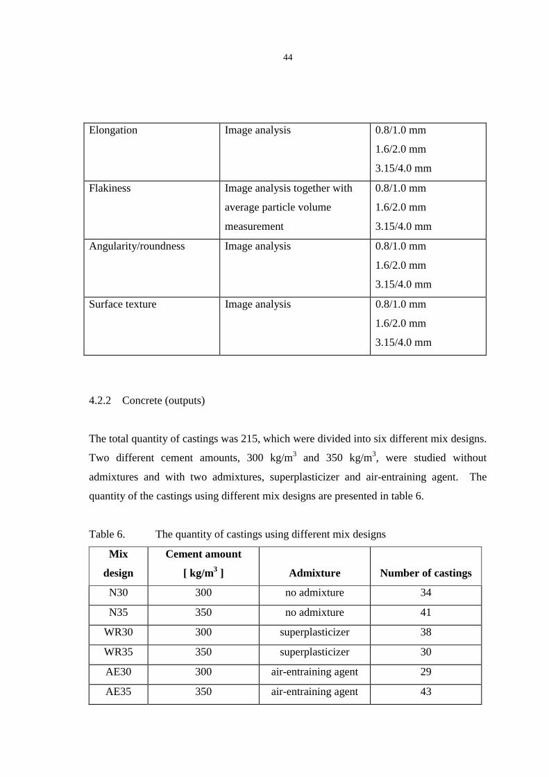
44
Elongation Image analysis 0.8/1.0 mm
1.6/2.0 mm
3.15/4.0 mm
Flakiness Image analysis together with
average particle volume
measurement
0.8/1.0 mm
1.6/2.0 mm
3.15/4.0 mm
Angularity/roundness Image analysis 0.8/1.0 mm
1.6/2.0 mm
3.15/4.0 mm
Surface texture Image analysis 0.8/1.0 mm
1.6/2.0 mm
3.15/4.0 mm
4.2.2 Concrete (outputs)
The total quantity of castings was 215, which were divided into six different mix designs.
Two different cement amounts, 300 kg/m3 and 350 kg/m3, were studied without
admixtures and with two admixtures, superplasticizer and air-entraining agent. The
quantity of the castings using different mix designs are presented in table 6.
Table 6. The quantity of castings using different mix designs
Mix
design
Cement amount
[ kg/m3 ] Admixture Number of castings
N30 300 no admixture 34
N35 350 no admixture 41
WR30 300 superplasticizer 38
WR35 350 superplasticizer 30
AE30 300 air-entraining agent 29
AE35 350 air-entraining agent 43

45
The drying shrinkage and weight loss measurements were mainly performed on mix
designs N35, WR30 and AE35 and there are therefore a greater number of castings with
these mix designs.
In order to determine deviations between castings, 15 % of them were repeated (see
appendix 2). In addition, two mixes were repeated several times (5 and 6 times) along the
castings to ascertain that no major changes had occurred during the one year that it took
to conclude all the castings.
As far as deviations within castings were concerned, the focus was on compressive
strength results. Each compressive strength result is an average of three (3) cubes; this
also applies to the results for density, because the same cubes were used for the density
measurements.
The concrete test programme consists of tests for both fresh and hardened concrete. The
tests were selected so as to cover the majority of the building code requirements and the
practical concrete tests performed during concrete production. They were also designed
to reveal potential difficulties arising from variations in the aggregate inputs. The lists of
tests are presented in tables 7 and 8 for fresh and hardened concrete respectively.
Table 7. Measured characteristics of fresh concrete and test methods
Concrete
characteristics Test method
Testing age
(after mixing) Remarks
Workability Slump
Flow value
5 min
7 min
All castings
All castings
Density of fresh concrete
Unit mass of the
concrete in 8 l container 10 min All castings
Air %, fresh concrete Pressure method 12 min All castings
Bleeding Bleeding test 10, 30, 60 min All castings

46
Table 8. Measured characteristics of hardened concrete and test methods
Concrete
characteristics Test method Testing age Remarks
Compressive
strength
Compressive strength
measurement
24 h
28, 91 d All castings
Density of hardened
concrete
Particle density 24 h
28, 91 d All castings
Drying shrinkage Measurement of
the length changes Up to 231 d
64 of 215
castings
Weight loss Measurement of
the weight changes Up to 231 d
64 of 215
castings
Air %,
hardened concrete
Determination from
the thin section 56 ± 2 d
(AE mix designs)
72 of 215 castings
Specific surface area
of air void
Determination from
the thin section 56 ± 2 d
(AE mix designs)
72 of 215 castings
Spacing factor
of air void
Determination from
the thin section 56 ± 2 d
(AE mix designs)
72 of 215 castings
4.3 Mix designs and concrete mixes, mixing procedure, test specimens
4.3.1 Mix designs and concrete mixes
Mix designs
Six (6) different mix designs were applied to all 215 castings, as shown in table 9. The
designs consisted of two different cement amounts, corresponding to low and high paste
volumes, together with three admixture classes; no admixture, superplasticizer or air-
entraining agent.

47
The mix designs were based on the following rules:
1. Two cement amounts, 300 and 350 kg/m3
2. Same water-cement ratio for both cement amounts
3. Both cement amounts without admixture (N), with superplasticizer (WR) and
with air-entraining (AE) agent
4. Same starting workability with one fines/semi-coarse aggregate combination in
low paste mix designs (B3/B14, slump 110±10 mm)
5. Same superplasticizer dosage % from the cement amount in the WR mix designs
6. Same air-entraining agent dosage % from the cement amount in the AE mix
designs
7. The water amount includes the water in the admixtures
8. Same fines % for the cement amount in all mix designs
9. Same combined grading curve for all mix designs, though fines amount (passing-
% 0.125 mm) varies according to rule # 8
Table 9. Mix designs
Mix
design
Cement
amount
[ kg ]
Water
[ l ]
Aggre-
gates
[ l ]
Fines
[ kg ]
20%C
Super-
plasticizer
[ kg ]
1.2%C
Air-entr.
1:19
[ kg ]
0.425%C
Air
[ % ]
W/C
ratio
Paste
amount
[ % ]
Paste
amount
[ % ]
w/ air
N30 300 195 700 60 - - 1 0.65 31.2 32.2
N35 350 228 651 70 - - 1 0.65 36.5 37.5
WR30 300 171 724 60 3.6 - 1 0.58 28.8 29.8
WR35 350 200 679 70 4.2 - 1 0.58 33.7 34.7
AE30 300 174 679 60 - 1.3 5 0.58 29.1 34.1
AE35 350 203 634 70 - 1.5 5 0.58 34.0 39.0
The mix designs were made with the assumption that the air % for the N and WR mix
designs would be 1% and for the AE mix designs 5%. However, it was known that there
would be great deviations between the actual measured values and the theoretical values.
Actually, this is one of the points of interest in this study, and it has to be taken into
account in the interpretation of the other results, e.g. compressive strength and
slump/spread values.

48
Combined grading curve
In all mix designs, the ratio of the fine and coarse aggregates was kept constant. The
percentage of the fine aggregate in the total aggregate was always 42.8 % and thus that of
the coarse aggregate was 57.2 % (5/10 mm 20.2 %-unit and 8/14 mm 37.0 %-unit). The
target combined grading curve for all the mix designs is presented in table 10. The
passing-% of the 0.125 mm sieve is dependent on the cement content and is further
slightly affected by the total aggregate amount of the mix designs. The target value varies
from 3.1% to 4.1%.
Table 10. Target combined grading curves for all mix designs
Mix
design
0.125
mm
0.25
mm
0.5
mm
1
mm
2
mm
4
mm
8
mm
14
mm
16
mm
N30 3.2
N35 4.0
WR30 3.1
WR35 3.8
AE30 3.3
AE35 4.1
8.9 15.0 23.0 32.5 46.5 60.0 95.0 100
Fine aggregate combinations
The fine aggregate products had been sieved into narrow size fractions: i.e. fines, 0/0.125
mm, and five semi-coarse fractions, 0.125/0.25, 0.25/0.5, 0.5/1.0, 1.0/2.0 and 2.0/4.0
mm.. Figure 11 presents the ways in which the fine aggregate fractions were combined.
The combination of the fines and semi-coarse fractions could range from:
• the same aggregate or
• two different aggregate products or
• a maximum of 4 different aggregate products both for the fines
and semi-coarse fractions

49
Figure 11. Combinations of the fine aggregate combining;fines and semi-coarse size fractions
Concrete castings
The list of all concrete mixes for the 215 castings with mix design type and fine
aggregate combinations is contained in appendix 2. The list also indicates repetitions of
castings.
4.3.2 Mixing procedure
The castings were mixed using a 50 litre Zyklos pan mixer, and the size of the batches
varied between 27 and 32 litres. A larger batch size was needed when shrinkage and
weight loss prisms were also cast.
The filling order of the mixer was: coarse aggregate products, cement and fine aggregate
products. The following figure 12, illustrates the mixing cycle. The total mixing time was
five minutes.
<0.125 mm
0.125 mm - 4 mm
A 100 %
A 100 %
A 100 %
B 100 %
C-D-E-Fmax 4 pc.
G-H-I-Jmax 4 pc.

50
Figure 12. Mixing cycle, total mixing time five minutes
4.3.3 Test specimens
For the purpose of compressive strength determinations, nine 100 mm cubes were cast
from each batch. The strength determinations were conducted on three ages: 24 h, 28 d
and 91 d, each representing an average of three cubes. The same cubes were used for
density measurements.
One additional cube was cast for the preparation of thin-section samples. An impregnated
pre-sample was made from each cube at the age of 56 ± 2 days, and only from the AE
mix designs were made final tin-section samples. Other pre-samples were stored as a
reserve information source in case some phenomenon might need extra clarification.
For the drying shrinkage and weight loss determinations, two 100 x 100 x 500 mm
prisms were needed. The determinations were made for 64 out of 215 castings. The
measurements consisted of drying shrinkage and weight loss determinations at ages of up
to 231 days.
Coarse aggregate, cement,fine aggregate
Dry mixing time,total 1 min
1 min
2/3 of the water
2 min
1/3 of the water +possible admixture
5 min
Wet mixing time,total 4 min
TOTAL MIXING TIME FIVE MINUTES

51
4.4 Testing methods and potential input values, aggregates
4.4.1 Mineralogical composition, fines and semi-coarse fractions
The mineralogical composition of the fine aggregate products was determined, using the
X-ray diffraction method, at the Geological Survey of Finland. For all the aggregates the
determination was made for two size fractions, <0.063 mm and 2.0/4.0 mm. Both size
fractions were ground to fine powder before sample preparation. The <0.063 mm size
fraction was additionally tested using two oriented mounts for enhanced determination of
clay minerals. From these concentrated and oriented samples the X�ray diffraction
spectrum was determined with the 2θ-angle region 2°-20°. After analysis, one sample
was treated with ethylene glycol for 24 hours and the other was heated for 1 hour at a
temperature of 550 °C. Following this, the X�ray diffraction spectrum was recorded for
the treated sample. By comparing the prior and post-treatment X�ray spectra with the
information obtained from infrared spectrometric analysis of untreated material, it was
possible to recognise and identify even minor quantities of clay minerals. A semi-
quantitative estimation of individual minerals was done by using experimentally obtained
absorption coefficients.
The potential input values gained from the mineralogical composition:
1. F and SC – clay, (clay amount, fines and semi-coarse), [ % ]
2. F and SC - mica, (mica amount, fines and semi-coarse), [ % ]
3. F and SC – amphibole, (amphibole amount, fines and semi-coarse), [ % ]
4. F and SC – quartz, (quartz amount, fines and semi-coarse) [ % ]
4.4.2 Specific surface area, fines
The specific surface area of the fines, <0.063 mm, was determined using a NOVA � 1000
Gas Sorption Analyser by the Quantachrome Corporation (BET method) and Coulter�s
LS Particle Size Analyser, which is based on the laser diffraction (LD) principle.

52
BET method
The basis of adsorption method is the fact that the amount of gas adsorbed on a gas-solid
interface under specific conditions is proportional to the interfacial area presented.
The most commonly used adsorption method is the adsorption isotherm derived by
Brunauer, Emmet and Teller (BET) using simplifying asusmptions; the isotherm gives
the amount n of gas adsorbed relative to the monolayer amount nm as a function of (1) the
gas pressure p divided by the saturation vapour pressure ps and (2) a constant C that
depends on the adsorption energy.
( ) ( )( )[ ] 1//1/1// −+−−= ssssm pCppppppCpnn Equation 6
The BET equation has generally been found to be very useful for physical adsorption for
non-porous solids, e.g. aggregates, in the pressure range 0.05 < p/ps < 0.35, and it is
usually satisfactory to determine just a single point near the upper limit of validity of the
BET isotherm. Since the constant C for nitrogen gas is generally much greater than unity
(generally 50-250), 1-p/ps, can be neglected compared with C p/ps, and the BET
adsorption isotherm is reduced to the relation:
( )sm ppnn /1−= Equation 7
The monolayer capacity nm can be calculated using equation Q* and the ideal gas
equation and thus, the equation becomes
( )sm ppRT
pVMn /1−= Equation 8
where,
p = ambient pressure (atm)
T = ambient temperature (°K)
R = gas constant (82.1 cc atm/°K mole)
V and p/ps are measured values

53
The total surface area St of the sample can be expressed as
MNAnS camt /= Equation 9
where,
N = Avogadro�s number (6.023 x 10²³ molecules/mol)
Aca = 16.2 Å2, cross-sectional area for the
hexagonal close-packed nitrogen at 77 °K (temperature of liquid nitrogen)
M = molecular weight of the adsorbate (nitrogen (N2) 28 g/mol)
By combining the equations Q* and Q* the total surface area equation becomes a form:
( )RT
pppVNAS scat
/1−= Equation 10
The degree of physical adsorption increases when temperature decreases. Thus, the
nitrogen gas is allowed to adsorb on the sample surface at the temperature of liquid
nitrogen (77 °K). When the sample is transferred to ambient temperature, the adsorbed
nitrogen gas starts to evaporate from the surface of the sample and this volume of
desorbed gas is measured (RUMPF1990). The specific surface area is obtained when the
total surface area is divided by the mass of the sample. Prior testing the samples were
dried at 80 º C.
LD method
Laser diffraction (LD) is a method where the particle size distribution is determined from
the light scattering information of different size particles.
A sample, which has been dispersed either in gas or liquid, is lead through a coherent
light (laser beam). When the coherent light meets the particle surfaces, the light scatters
and thus, a diffraction pattern is formed. Both the scattered and unscattered light is then
focused to a detector plane through a transform lens, figure 13.

54
Figure 13. Optical arrangement of laser diffraction method to obtain size distribution
of particles (FELTON 1990)
The unscattered light is focused to a point on the optical axis and the scattered light
forms a pattern of rings around the central spot. The diffraction pattern is the net
diffraction of all the separate particles. Movement of the particles does not cause
movement of the diffraction pattern, because light scattered at an angle θ, will always
give the same radial displacement in the detector, irrespective of the particles position in
the illuminating beam. This diffraction pattern produced is known as the Fraunhofer
diffraction pattern. From the diffraction pattern can thus, be determined the particle size
distribution. (FELTON 1990, STANLEY-WOODS AND LINES 1992)
In the Fraunhofer diffraction calculations, it is assumed that all the particles are spheres.
As the spheres are the only particles having an equal diameter when measured either
from projected area or volume, it is obvious that the shape of the particles affect the
achieved result. For irregular particles the grading result depends on the orientation of the
particles. The particles are detected as a set of spheres having the average diameter
between the smallest and largest projected area diameter thus, generally causing wider
span in the grading curve and possibly transfer of the average particle diameter.
(WEICHTER 1986)
The samples were tested in water dispersion. To ensure proper dispersion the samples
were first wetted in a beaker by a small amount of water after which the beaker was
placed in an ultrasonic bath for one minute.

55
The main difference between the two methods is that the BET method determines the
actual surface area, including the surface area of accessible pores, by measuring the
amount of adsorbed gas on the gas-solid interface, while in the LD method the area is
calculated from the grading curve, with the assumption that all the particles are spheres
and non-porous.
The potential input values are (used denotation in bold):
1. F - BET value (specific surface area by BET, fines), [m2/g]
2. F - LD value (specific surface area by LD, fines), [m2/g]
4.4.3 Grading, fines
The grading of the fines, <0.063mm, was determined by means of laser diffraction
analysis. The equipment used was a Coulter LS Particle Size Analyser.
The principle of the method is described in chapter 4.4.2.
The potential input values are (used denotation in bold):
1. F - Hf, [%], is the sum of the passing-% for sieve sizes of
2, 4, 8, 11.2, 16, 22.4, 31.5, 45, 63, 80, 125 µm, fines
2. F - 0.008 mm, [% ], is the passing-% for the sieve size of 8 µm, fines
3. F - Cu, [ - ], is the ratio of the sieve sizes for which the passing-% is 60% and
10%, fines
4.4.4 Particle density, fines and semi-coarse fractions
The particle density measurements were made for size fractions <0.063 mm and 2.0/4.0
mm using a Quantachrome helium pycnometer, AccuPyc 1330.
The principle of the Helium pycnometer method is that the volume of a sample is
determined by measuring the pressure change of helium in a calibrated volume. The

56
density can be calculated when the mass of the sample is given. Prior testing the samples
were dried at temperature of 80 º C.
The potential input values are (used denotation in bold):
1. F – density (particle density, fines), [ Mg/m3 ]
2. SC – density (particle density, semi-coarse fractions), [ Mg/m3 ]
4.4.5 Particle porosity, fines and semi-coarse fractions
The particle porosity values are based on mercury intrusion porosimetry measurements
and were conducted using a Micrometrics Poresize 9320. The determinations were made
for the size fractions <0.063 mm and 0.5/1.0 mm.
The principle of the method is based on the fact that mercury behaves as a non-wetting
substance towards most materials. Consequently, it does not penetrate into the pores of
the material and one must apply pressure to make it do so. The most commonly applied
intrusion equation is the Washburn equation, which states that the pore size is inversely
proportional to the applied pressure:
( ) Pr LV /cos2 θσ= Equation 11
where,
P = pressure applied to the mercury
LVσ = surface tension of the mercury surface
θ = contact angle of the mercury
r = radius of the capillary
If the mercury intrusion method is applied to loose powder material, the result obtained
includes both the accessible pores in the particles (intra-particle voids) as well as the
voids between the particles (inter-particle voids). However, if the loose material is of
single size, granular material the mercury fills the inter-particle voids space
predominantly without pressure (VAN BRAKEL ET AL. 1981, KLOUBEK 1994) and thus, the
result obtained represents intra-particle voids, i.e. particle surface porosity. The former

57
case applies to the tested aggregate fines (<0.063 mm) and the latter case to the tested
aggregate semi-coarse fraction 0.5/1.0 mm.
A contact angle of 130.0° and a surface tension of 485 mN/m were used in the
calculations. Prior testing the samples were dried at 105 °C and then evacuated in a
penetrometer before mercury filling to minimum 3 Pa. The measured range of pores was
from 300 µm (3 Pa) down to 6 nm (200 MPa).
The potential input values are (used denotation in bold) :
1. F – avg. pore size (average pore size, fines), [µm]
2. F – tot. pore area (total pore area, fines), [ m2/g ]
3. SC – avg. pore size (average pore size, semi-coarse), [µm]
4. SC – tot. pore area (total pore area, semi-coarse), [ m2/g ]
5.-7. SC – pore area 60-300Å/300-900Å/>900Å
(incremental pore area 60-300Å, 300-900Å and >900Å, semi-coarse), [ m2/g ]
4.4.6 Zeta potential, fines
The Zeta potential measurements were performed for the fines, <0.063 mm, using a
Coluter Delsa 440.
Because the zeta potential measures the average electric charge of the aggregate particle
surfaces, the tests were carried out for samples without admixtures (N), with
superplasticizer (WR) and with air entrainment agent (AE). The dosages of the
admixtures were according to the mix designs, i.e. 0.2% and 0.07% from the amount of
aggregate for the WR and AE measurements respectively.
In order to obtain results that can be related to the environment of the concrete, the
electrolyte was made of 4 litres of ion-exchanged water and 1.00 kg of cement. After
mixing, the electrolyte was filtered twice, first with a coarse filter and then with a 0.22
µm membrane filter. The pH value of the electrolyte was 12.5. The zeta potential

58
measurements were conducted by means of the following routine: 100 mg of fines was
added to a beaker containing 100 ml of electrolyte. The beaker was placed in an
ultrasonic bath for one minute to ensure proper dispersion, after which the beaker was
placed on a magnetic stirrer. The sample was allowed to balance itself for 10 minutes
before measurements were made. Before any admixture addition, the N (no-admixture)
value was measured to ensure that the sample was clean of any impurities. After the
admixture had been added, the sample was again allowed to balance itself for 10 minutes
before measurements were conducted.
The potential input value is (used denotation in bold):
1. F - Zeta pot. (Zeta potential value, fines), [ mV ]
4.4.7 Resistance to fragmentation, semi-coarse fractions
The European standard EN 1097-2: Methods for the determination of resistance to
fragmentation was applied. A slight modification was made to the tested size fraction, i.e.
the size fraction was 4.0/5.6 though the smallest size fraction given in the EN standard is
4.0/8.0 mm. The shape properties of the aggregate products were not altered, e.g. by bar
sieving, and thus the results resemble the product characteristics and not only the raw
material characteristics.
The potential input value is (used denotation in bold):
1. SC - LA value (mod.) (Los Angeles value (mod.), semi-coarse), [ % ]
4.4.8 Elongation, flakiness, particle volume and quantity, semi-coarse fractions
The determination of elongation, flakiness, particle quantity, surface area, angularity and
surface texture area were all based on scanned images. The scanner was a normal office
scanner (AGFA SnapScan 600). For image processing, an image analysis tool was
developed.

59
The pre-processing of the scanned images
The images were scanned in colour, and thus they are first converted to greyscale. The
aggregate particles are recognised from the background using simple thresholding. The
grey level distribution of the image has two peaks, one corresponding to the background
and one to the particles. The minimum between the two peaks in the histogram marks the
decision boundary: pixels which are darker than this boundary belong to the background
and pixels which are lighter belong to particles. In order to reduce noise, the binary
image produced by means of thresholding is then filtered using a 3-by-3 median filter.
This operation marks each pixel black or white, depending on which was more common
in the pixel�s 3-by-3 neighbourhood. Next, a morphological opening operation is
performed. This tends to even out the particle boundaries and removes small holes,
caused by speckles in the image, from the particles. Finally, connected areas in the image
are sought and holes possibly still left inside these areas are filled.
The determinations of elongation and flakiness were conducted for three narrow size
fractions: 3.15/4.0, 1.6/2.0 and 0.8/1.0 mm. The same procedure was applied in the case
of each size fraction:
a. The theoretical geometric mean for the sphere diameter of the narrow size
fraction was calculated (e.g. 3.15/4.0 mm → 3.55 mm)
b. Particles of the narrow size fraction were spread on a scanner screen
c. The image of the particles was scanned with a resolution of 1000 pixels per inch
d. The quantity and the areas of the particles were determined by an image analysis
program. (The quantity was cross-checked by manual counting)
e. The average area of one particle from the narrow aggregate size fraction was
calculated and the pixels were transformed to mm value
f. From the average area was calculated
the average equivalent 2D diameter (=circle)
h.
g.
ELONGATION =[ avg. equivalent 2D diameter / theoretical sphere diameter ]
As the quantity of the scanned particles and the particle density are known → the
average particle volume → the average equivalent 3D diameter (=sphere)

60
The part
means o
( Total a
The perc
was the
8.0% fo
The elo
aggrega
The pote
1. S
(
2. S
(
3. S
(
4. S
(
5. S
4.4.9 A
Angular
approxim
shaped
pixels fr
i.
FLAKINESS =[ avg. equivalent 2D diameter / avg. equivalent 3D diameter ]
icle quantity per each size fraction was calculated from the mix information by
f the equation:
mount of aggregates [ l ] * Percentage of size fraction [ % ] )
Average particle volume of size fraction [ dm3 ]
entage of the size fraction was calculated from the combined grading curve and
same for all mix designs i.e. 14.0% for 3.15/4.0 mm, 9.5% for 1.6/2.0 mm and
r 0.8/1.0 mm. The total amount of aggregate can be seen from table 9.
ngation, flakiness and quantities was calculated for each mix according to the
te combination and mix design.
ntial input values are (denotation in bold):
C – Elng 3.15/4.0, 1.6/2.0 and 0.8/1.0 mm
Elongation of size fractions, 3.15/4.0, 1.6/2.0 and 0.8/1.0 mm), [ - ]
C – Flkn 3.15/4.0, 1.6/2.0 and 0.8/1.0 mm
Flakiness of size fractions, 3.15/4.0, 1.6/2.0 and 0.8/1.0 mm), [ - ]
C – Qnty 3.15/4.0, 1.6/2.0 and 0.8/1.0 mm
Particle quantity of size fractions, 3.15/4.0, 1.6/2.0 and 0.8/1.0 mm), [ - ]
C- Surface area 3.15/4.0, 1.6/2.0 and 0.8/1.0 mm
Surface area of size fractions, 3.15/4.0, 1.6/2.0 and 0.8/1.0 mm), [ - ]
C – tot. surface (total surface, semi-coarse), [ - ]
ngularity/roundness, semi-coarse fractions
ity is determined from the morphological spectrum of the particle and is
ated by performing successive morphological �eroding� operations using disk-
masks. The �eroding� operation rounds the edges of the particles and removes
om the particle, depending on the size of the mask and the ruggedness of the

61
border. The features are computed using masks with radii of 3, 5, 7, 10 and 12 pixels.
The number of pixels eroded from the stone is then divided by the square of the mask
radius. As a result a sequence of five numbers is acquired, representing the shape
distribution of the stone border. An average of the five-number sequence was calculated,
and for the purpose of input parameter, the angularity was additionally averaged
according to the particle quantity of the three size fractions. (GONZALES AND WOODS
1993)
Angularity is computed with regard to each aggregate particle independently. The results
of a given image are then the expectation values of the independent particles.
The potential input value is:
1. SC – Angularity (angularity, semi-coarse), [ - ]
4.4.10 Surface texture, semi-coarse fractions
When the surface texture is determined, a square is fitted inside the aggregate particle
and texture inside the square is considered. Because the size of the texture samples varies
from particle to particle, the texture sample is copied periodically so that samples from
different particles become comparable. A two-dimensional Fourier transform is
computed from the texture sample. In the two-dimensional case the Fourier transform
coefficients are too numerous to be useful alone as features. Instead, radial sums of the
absolute values of the Fourier transform coefficients from [pi/2..pi/4] band is used. The
input parameter was calculated as the weighed average of the particle quantity of the
three particle sizes. (JAIN 1989)
The surface texture is computed with regard to each aggregate particle independently.
The results of a given image are then the expectation values of the independent particles.
The potential input value is:
1. SC - Surface texture, (surface texture, semi-coarse) [ - ]

62
4.5 Testing methods and concrete output values
All concrete castings were made and tests conducted at the Fortum concrete laboratory in
Vantaa, except in the case of the thin-section analyses, which were carried out at the
Finnish Research Centre in Otaniemi.
4.5.1 Workability
For workability determination, the slump and flow value was applied according to testing
methods ISO 4109 and SFS 5286 respectively (figure 14). The slump was measured 5
and 15 minutes and flow values 7 and 17 minutes after the mixing.
Figure 14. The measuring of the slump
and flow value
The outputs are:
1. Slump 5 min, [ mm ]
2. Flow value 7 min, [ mm ]

63
4.5.2 Air % and density of fresh concrete
The testing of the percentage of air in the concrete was performed according to the
standard ISO 4848, as shown in figure 15. The testing was done 12 minutes after the
mixing. Prior to the air % measurement, the 8 litre vessel filled with concrete using
standard compaction routines was weighed, and in this way the unit density of the fresh
concrete was determined.
Figure 15. Measurement of the air % of fresh concrete
The testing method for the air % measures all the air in the concrete: entrapped and
entrained air. Therefore no judgement of the quality of the air can be made on the basis
of this measurement. Consequently, thin-sections were made from the AE castings for
the air parameter determinations (see 4.5.6).
The outputs are:
1. Air %, fresh concrete, [ % ]
2. Density of the fresh concrete, [ kg/m3 ]
3. Excess density of the fresh concrete, [ % ] (deviation from the theoretical density)

64
4.5.3 Bleeding
The measurement of bleeding was done after intervals of 10 min, 30 min and 60 min.
Approximately 2 litres of concrete was put into a plastic cylinder container and vibrated
slightly. The container was covered with a lid and placed in a quiet place to rest. After a
specified time the bleeding water was sucked out and weighed. The bleeding was
calculated by means of the equation:
Bleeding = Vw / V, Equation 12
where
Vw = the amount of bleeding water, [ g ]
V = the volume of the concrete
With some concrete mixes, it was difficult to measure the bleeding water accurately due
to the large overall amount of bleeding and the segregation tendency of the concrete. The
bleeding liquid consisted of both water and very low viscosity cement paste, and hence
the “choice” of the liquid was some times challenging.
The outputs are:
1. Bleeding 10 min, [ g/cm3 ]
4. Bleeding 30 min, [ g/cm3 ]
3. Bleeding 60 min, [ g/cm3 ]
4.5.4 Compressive strength and density of the hardened concrete
The compressive strength and density were determined at the ages of 24h, 28d and 91d.
All the values are average for three 100 mm cubes. The density determinations were
made as mass per volume calculations based on weighing the specimen in air and in
water (figure 16).

65
Figure 16. Density determination of the hardened concrete
The 28d and 91d specimens were stored in a climate room with RH >95% and
temperature 20 ± 2 °C. At the testing age the specimens were taken out of the climate
room 3 hours before testing.
The outputs are:
1 – 3. Compressive strength 24h, 28d and 91d, [ MPa ]
4 – 6. Standard deviation of the compressive strength 24h, 28d and 91d, [ MPa ]
7 – 9. Density 24h, 28d and 91d, [ kg/m3 ]
10–12. Standard deviation of the density 24h, 28d and 91d, [ MPa ]
13-15. Excess density 24h, 28d and 91d, [ % ] (deviation from the theoretical density)

66
4.6 Testing methods for drying shrinkage, weight loss and air parameters,
hardened concrete
4.6.1 Drying shrinkage and weight loss
For drying shrinkage and weight loss determinations two 100 x 100 x 500 mm prisms
with measuring bolts in the ends were cast. After demoulding, the prisms were placed in
water for curing for 6 days before weight and length measurements were conducted;
these were set as the zero values for the drying shrinkage and weight loss determinations.
The prisms were stored in a climate room with RH 40 ± 3 % and temperature 20 ± 2 °C.
Weight and length determinations were done at the ages of 14, 21, 35, 49, 63, 91, 119,
147, 175, 203 and 231 days. A general view of the climate room and of the set-up for the
length measurement can be seen in figures 17 and 18.
Figures 17. General view of the drying shrinkage climate room (left)
Figure 18. Set-up for the drying shrinkage measurement (right)

67
4.6.2 Thin section analysis; air %, specific surface area and spacing factor of air void
From all the castings one thin-section pre-sample was made by cutting a 30x50x10 mm
prism vertically from the middle of a 100 mm cube. The pre-samples were impregnated
with clear resin at normal atmosphere pressure, and thus the reactions in the concrete
were interrupted. Final petrographic thin sections were prepared from all the AE castings.
The pre-samples were vacuum impregnated with fluorescent coloured resin and glued on
slides. Finally the samples were diamond cut and grind down to sizes 30x50 mm2 x 25
µm. A detailed description of the preparation method is contained in standard NT Build
381.
The analyses were performed using a Leica DM LP polarisation and fluorescence
microscope, applying the modified point-count method described in standard ASTM
C457 (NT Build 381). Air pores which had diameter < 0.8 mm were counted as air voids
and pores with greater diameter as entrapped air pores. The minimum analysed air pore
size was with diameter 0.020 mm. The analysed parameters were: air void percentage,
entrapped air percentage, specific surface of the air voids (mm2/mm3) and spacing factor
of the air voids (mm).

68
5. AGGREGATE TEST RESULTS AND DISCUSSION
The test programme was constructed in such a way that the fines, < 0.125 mm, and the
semi-coarse fraction, 0.125/4 mm, could be interpreted separately. This is vital. The
reason is that, although the testing methods for these two groups are different, the test
results can correlate quite strongly, and thus one phenomenon can hide the other. As two
examples one may give the results of the F-LD specific surface area for rock products vs.
the SC- Los Angeles value and the F- BET specific surface area for gravel products vs.
the SC- total pore area (figures 19 and 20).
Figures 19 and 20. Correlations between the fines and the semi-coarse fractions;
Examples: F- LD vs. SC- Los Angeles and
F- BET vs. SC-total pore area
It is inevitable that there will be fines and semi-coarse inputs such that the separate fines
inputs will correlate with each other; the same applies to the semi-coarse fraction inputs.
The correlations between the inputs are taken into account in the Excel program for the
prediction of fine aggregate�concrete interaction by Principal Component Analysis (see
chapter 3). Appendix 3 provides lists of the correlations within the fines and semi-coarse
inputs.
LD SSA fines vs Los Angeles value (mod.)A -aggregate
R = 0.91
15
20
25
30
35
40
45
0.2 0.3 0.4 0.5
LD specific surface area [m2/g]
Lo
s A
ng
eles
val
ue [
%]
BET SSA fines vs Total pore area SC B - aggregate
R = 0.97
0
0.1
0.2
0.3
0.4
0 5 10 15BET specific surface area [m2/g]
To
tal p
ore
are
a [m
2 /g]

69
5.1 Mineralogical composition
The X�ray diffraction determinations are only semi-quantitative and thus the actual
quantities are difficult to determine with high precision. The results from the
determinations are presented in table 12-14 with an accuracy of within 1%�unit for the
lower concentrations (<10 %) and 5 %-unit for the higher concentrations (≥ 10%).
Table 12. Mineralogical composition for the rock products; X-ray determination
A2
[%]
F SC
A3
[%]
F SC
A6
[%]
F SC
A7
[%]
F SC
A8
[%]
F SC
A10
[%]
F SC
A15
[%]
F SC
A16
[%]
F SC
Quartz 7 40 40 35 15 30 35 45 10 25 4 15 4
Potassium feldspar 30 30 30 30 15 20 8 9
Plagioclase 35 30 25 35 30 40 35 30 80 60 30 45 75
Hornblende 1 45 6 5 10 65 20 20
Biotite 3 1 1 1 10 6 2 15 8 7 7 4
Chlorite 1 2 1 1 4 3 1 1 3
Carbonate 15
Pyroxene 15
Garnet 2 2
Table 13. Mineralogical composition for the B1-8 gravel products; X-ray determination
B1 [%]
F SC
B2 [%]
F SC
B3 [%]
F SC
B6 [%]
F SC
B7 [%]
F SC
B8 [%]
F SC
Quartz 20 30 35 35 35 15 20 20 35 45
Potassium feldspar 15 25 10 20 25 8 8 20 10 25
Plagioclase 25 30 30 40 35 20 40 50 35 30
Hornblende 4 3 2 3 10 8 5
Biotite 10 2 2
Muscovite 6 10 10 1 3
Chlorite 1 2 10 7 4 7 1
Smectite 20 25 9 5
Kaolinite 15 2
Vermiculite 4 1
Talc 1 2

70
Table 14. Mineralogical composition for the B9-14 gravel products; X-ray determination
B9 [%]
F SC
B10 [%]
F SC
B11 [%]
F SC
B12 [%]
F SC
B13 [%]
F SC
B14 [%]
F SC
Quartz 55 40 35 25 30 25 20 40 35 25
Potassium feldspar 10 20 8 35 10 20 10 20 15 30
Plagioclase 20 30 30 40 35 45 30 30 35 40
Hornblende 2 8 6 3 3 2 5 1
Biotite 3 1 2 1 1
Muscovite 3 15 1 15 2 2
Chlorite 5 6 1 6 3 8 6 3 1
Smectite 5 2 15
Kaolinite 7
Vermiculite 7
Talc 2
The mineralogical composition of the SCF and the fines can vary substantially both with
the rock and the gravel products (tables 12-14). For the rock products, the reasons for the
deviation lie in the heterogeneous of the rock product itself, enriching of minerals during
the crushing process and representativeness of the samples. The gravel products, on the
other hand, have been through weathering processes and hence the mineralogical
composition, especially of the fines, has changed during a long period. The weathering of
the gravel products can indirectly be measured, e.g. using the BET method, and as
general, such products which have larger amounts of clay minerals show also higher
values in the BET determination.
5.2 Grading
The measurements were performed on three test specimens and each specimen being
determined twice. The average coefficient of variation of the surface area (calculated
from the grading information) was 4.6 ± 1.9%.

71
The potential input values i.e. fineness, shape of the grading curve and one passing-%
value (0.008 µm), were chosen so that the grading curve could be described by them and
its orientation would be unambiguous.
Figure 21 illustrates the three potential input values from the grading curve for each of
the fines. The scatter in the values was in general greater for gravel products than for
rock products. Thus, the lowest and highest fineness values for the gravel and crushed
rock products were 338 (B14) � 644 (B11) and 425 (A8) � 636 (A15) respectively. The 8
µm passing-% values varied with the gravel products within the range of 5.9% (B3) and
34.6% (B11), whereas the rock products had values within the range of 13.0% (A8) and
27.9% (A15). Furthermore, the Cu values for the gravel products varied from 3.4% (B3)
to 16.5% (B10) and for the rock products from 10.1% (A8) to 16.2% (A3). The mix
values for the grading inputs were calculated proportional to the percentage of the
different fines.
Figure 21. Values for fineness, 8µm passing-% and Cu for each of the fines
Fineness, 8 µm passing-%, Cu
0
100
200
300
400
500
600
700
800
900
B1
B2
B3
B6
B7
B8
B9
B10
B11
B12
B13
B14 A2
A3
A6
A7
A8
A15
A16
Fines
Fin
enes
s
0
5
10
15
20
25
30
35
408
µm p
-% a
nd
Cu
Fineness
8 µm p-%
Cu

72
Figures 22 and 23 show the grading curves of the finest and coarsest gravel and rock
fines. Figure 22 presents the cumulative grading curve and the figure 23 shows the same
information in differential format.
Figure 22. Cumulative grading curves of A8, A15, B3 and B11 products, fines
Figure 23. Differential grading curves of A8, A15, B3 and B11 products, fines
Cumulative grading curve
0102030405060708090
100
0.01 0.1 1 10 100 1000Particle diameter [µm]
Vo
lum
e [%
]
A08
A15
B03
B11
Differential grading curve
0
2
4
6
8
10
0.01 0.1 1 10 100 1000
Particle diameter [µm]
Vo
lum
e [%
]
A08
A15
B03
B11

73
As can be seen from figure 22, the shape of the cumulative grading curves for the rock
products are very similar to each other. In contrast, the shape of the cumulative grading
curves for the gravel products vary considerably. This could of course be due to the
choice of test material, but more likely, it results from the classification actions caused by
the glacial periods and proceeded weathering. The rock products have been subjected
only to compressive stressing processes, and thus the fines generated fall within narrower
grading limits, (RUMPF 1990). The differential grading curve of the B11 reveals that the
product has a fairly large amount of clay-size particles and thus indicates weathered
material. This can additionally be seen from the SEM pictures, figures 24, of the fines as
well as from their surface area values (see 5.3).
B11
A15
B3
A8
Figure 24. SEM pictures of the fines B3, B11, A8 and A15. Magnification x 500.

74
The SEM pictures also accord well with the fineness and Cu values of the fines. What can
also be seen from the pictures is the shape properties of the fines. The gravel particles
mainly have a cubical shape, whereas the rock particles are often flaky and/or elongated.
The structure, mineral size and mineralogical composition of the rock has a vast
influence on the shape of the particles. The exact amount of the crushed fines was known
but was not used as a potential input, as in the everyday production it would not be
possible to determine it.
5.3 Specific surface area
The LD measurements were made 3*2 times (see 5.2) and the BET measurements three
times. The average coefficient of variation was for the LD 4.6 ± 1.9% and 11.0 ± 9.2%
for the BET.
The specific surface area of the fines was determined by means of two methods: gas
adsorption (BET method) and laser diffraction (LD). Of these two, the gas adsorption
method can be considered a direct method and laser diffraction as an indirect method (see
4.4.2). The BET values of the fines varied between 1.77 m2/g (B3) and 13.98 m2/g (B10)
for the gravel products and between 1.25 m2/g (A8) and 2.73 m2/g (A15) for the rock
products. The corresponding LD values of the fines varied from 0.223 m2/g (B3) to 0.633
m2/g (B11) for the gravel products and from 0.259 m2/g (A8) to 0.682 m2/g (A15) for the
rock products. Figure 25 shows the results obtained from both determinations.

75
Figure 25. Specific surface area values determined using the BET�method and LD
The LD value describes the grading/fineness of the fines as one value. Because the
method calculates the surface area, i.e. constitutes indirect determination, and assumes
the particles to be spheres, it can be concluded that the value does not contain any
information on the particle shape or the weathering properties of the fines. As BET is a
direct method, it contains both types of information, although weathering is more
prominent than the shape properties. In practice, this means that the BET value should be
considered when the water-cement ratio of the mixes is determined with the bone-dry
state of the aggregate products. Consequently, the LD surface area value should be
considered when the w/c ratio is based on the saturated-surface dry (SSD) state of the
aggregate products. Figure 26 shows pictures of the B10 and A7 fines that have close LD
values, 0.444 m2/g and 0.475 m2/g, but very different BET values, 13.98 m2/g and 2.44
m2/g.
Specific surface area
0
2
4
6
8
10
12
14
16
B1
B2
B3
B6
B7
B8
B9
B10
B11
B12
B13
B14 A2
A3
A6
A7
A8
A15
A16
Fines
BE
T [
m2 /g
]
0.0
0.1
0.2
0.3
0.4
0.5
0.6
0.7
0.8
LD
[m
2 /g]
BET
LD

76
B10 A7
Figure 26. SEM pictures of the fines B10 and A7. Magnification x 1500
The correlation between LD and BET is non-significant (R = 0.22), but if the gravel and
rock products are interpreted as separate groups the correlation for rock products
becomes significant (R= 0.76). The reason becomes clear if we consider the fact that the
rock products are virtually non-weathered and that the main difference between the LD
and BET results is thus due to the shape properties of the particles.
5.4 Particle density
The average coefficient of measurement variation was 0.12 ± 0.03% and was determined
from 12 aggregate fractions, 9 SCF and 3 fines. The determinations were carried out
with three test specimens and each specimen was measured three times (3 x 3 times).
The remaining 23 aggregate fractions were measured 1x 3 times.
Fines
The particle density values for the fines were quite constant for the gravel products. The
values varied between 2.681 Mg/m3 (B3) and 2.797 Mg/m3 (B7). Greater variation, from
2.654 Mg/m3 (A2) to 3.015 Mg/m3 (A15), was observed in the fines of the rock products
Figure 27 presents the particle density values for each fines.

77
Figure 27. Particle density values for the fines
Semi-coarse fractions
The gravel products showed a small scatter in the particle densities of the semi-coarse
fractions. The lowest value was 2.647 Mg/m3 (B8) and highest 2.726 Mg/m3 (B7). For
rock products, the scatter was greater: between 2.636 Mg/m3 (A3) and 3.008 Mg/m3
(A16). The results are presented in figure 28.
Rock quarries are normally quite heterogeneous when it comes to rock types, and hence
it is possible for particle density to vary significantly from one rock type to another. For
example, a difference of 0.15 Mg/m3 in particle density (2.80 Mg/m3 instead of 2.65
Mg/m3) in normal concrete with 1750 kg of aggregate affects the volume of 1 m3 by �3.6
percentage, i.e. -36 litres/m3.
Particle density
2.4
2.5
2.6
2.7
2.8
2.9
3.0
3.1B
1
B2
B3
B6
B7
B8
B9
B10
B11
B12
B13
B14 A2
A3
A6
A7
A8
A15
A16
Fines
Den
sity
[M
g/m
3]

78
Figure 28. Particle density values for the semi-coarse fractions
5.5 Particle porosity
The measurements were performed 2-6 times for each aggregate product (fines and SCF)
and the average coefficients of measurement variation thus obtained are shown in table
15.
Table 15. Average coefficient of particle porosity measurement variation
Average coefficient of measurement variation
Fines SCF
Average pore size 8.7 ± 9.2% 14.0 ±12.5%
Total pore area 6.9 ± 7.3% 17.7 ± 17.1%
As can be seen from table 15, the accuracy is substantially better for the fines than for the
SCF. This is mostly due to the disproportion between the sample size and the fraction
size i.e. the sample size was 1-2 g and the tested semi-coarse size fraction was 0.5/1.0
Particle density
2.4
2.5
2.6
2.7
2.8
2.9
3.0
3.1
B1
B2
B7
B8
B10
B11
B12
B13
B14
RE
F
A2
A3
A7
A8
A10
A16
Semi-coarse
Den
sity
[m
g/m
3 ]

79
mm. This equals approximately 100 grains. The sample size is same for the fines, which
has size fraction <0.063 mm.
The weathering of the aggregates dissolves minerals, i.e. increases particle porosity,
disintegrates particles and causes mineral transformation. Hence, it is to be expected that
several potential input values will correlate with the particle porosity values. The data
source for the total pore area and average pore size is the same, and thus it is obvious that
they display a good correlation (figure 29) .
Figure 29. Correlations between average pore size and total pore area for the
fines and semi-coarse fractions
Fines
The total pore area and average pore size values for the fines are presented in figure 30.
The gravel products showed greater scatter in the values than did the rock products. For
the total pore area, the gravel products had values between 0.218 m2/g (B14) and 3.574
m2/g (B10), and the rock products showed values between 0.572 m2/g (A6) and 1.031
m2/g (A7). The smallest and largest average pore size values for the gravel and rock
products were 0.459 µm (B10) - 5.230 µm (B14) and 1.420 µm (A7) � 2.514 µm (A8)
respectively.
Avg pore size vs total pore area, fines
y = 1.5078x-1.1469
R = 1.00
0.0
1.0
2.0
3.0
4.0
0.0 1.0 2.0 3.0 4.0 5.0 6.0
Average pore size [µm]
To
tal p
ore
are
a[m
2 /g
]
Avg pore size vs. total pore area,semi-coarse
y = 0.1404x-0.9831
R = 0.98
0
0.1
0.2
0.3
0.4
0.5
0 2 4 6 8 10 12
Average pore size [µm]
To
tal p
ore
are
a [m
2 /g]

80
Figure 30. Average pore size and total pore area for the fines
A correlation between the total pore area and the BET surface area in the case of fines of
the gravel products is also to be expected, because the molecular area of the nitrogen gas
(16.2 Å2) is much smaller than the smallest pore size diameter (0.006 µm = 60 Å) as
measured by means of mercury intrusion (figure 31). The rock products are not
weathered, and so there is no statistically significance correlation between the total pore
area and the BET value (figure 31).
Figure 31. Correlations between BET value and total pore area, fines
Average pore size and total pore area
0
1
2
3
4
5
6
7B
1
B2
B3
B6
B7
B8
B9
B10
B11
B12
B13
B14 A2
A3
A6
A7
A8
A15
A16
Fines
Avg
po
re s
ize
[µm
]
0.0
0.5
1.0
1.5
2.0
2.5
3.0
3.5
To
tal p
ore
are
a [m
2 /g]
Avg pore size
Total pore area
BET (A) vs total pore area
R = 0.62
0.5
0.6
0.7
0.8
0.9
1.0
1.1
1.0 1.5 2.0 2.5 3.0
BET value [m2/g]
To
tal p
ore
are
a [m
2 /g]
BET (B) vs total pore area
R = 0.96
0.0
1.0
2.0
3.0
4.0
5.0
0.0 5.0 10.0 15.0
BET value [m2/g]
To
tal p
ore
are
a [m
2 /g]

81
For powders, i.e. fines, the mercury intrusion method measures not only the particle
porosity but also the pore size distribution and space/voids between the particles (see
4.4.5). The quantity of voids is dependent on the packing degree of the powder. The main
factors affecting the packing degree of the powders are the grading curve, particle shape
and surface adhesion (CUMBERLAND 1987, RUMPF 1990). The Cu value describes the
shape of the grading curve and the linear correlation between the average pore sizes and
the Cu value is 0.91 for the rock products and 0.89 for the gravel products.
Semi-coarse fractions
The highest total pore areas were 0.337 m2/g (B1) and 0.058 m2/g (A7) for the semi-
coarse fractions of the gravel and rock products respectively (figure 32). The lowest
value for the rock products was 0.017 m2/g (A8 and A10) and for the gravel products
0.010 m2/g (B14). The highest average pore sizes were 10.43 µm (A8) and 9.08 µm
(B14) for the rock and gravel products respectively. The lowest values were 0.36 µm
(B1) for the gravel product was and 2.94 µm (A7) for the rock product.
Figure 32. Total pore area and average pore size for the semi-coarse aggregates
Total pore area and average pore size
0
2
4
6
8
10
12
A2
A3
A7
A8
A10
A16 B
1
B2
B7
B8
B12
B13
B14
B15
RE
F
Semi-coarse aggregate
Avg
. p
ore
siz
e [u
m]
0.00
0.06
0.12
0.18
0.24
0.30
0.36
To
t. p
ore
are
a [m
2 /g]
Average pore sizeTotal pore area

82
The total pore area of the semi-coarse fractions is divided into three categories: pore sizes
> 0.09 µm, 0.03�0.09 µm and 0.006�0.03 µm. As can be seen in figure 33, only the
gravel products have pores in the smallest category.
Figure 33. Incremental pore areas for the semi-coarse aggregates
What is noteworthy is that those gravel products that are partly crushed do not contain
the smallest pores and only rock products that have been stored in outdoor stockpiles for
years have the middle-category pores. It is quite likely that for the gravel products, the
crushing process has partly shaken off the most weathered layer, and//or that this layer
has partly flaked off during the crushing. The particle porosity origin from the weathered
layers exist in the aggregate product even after the crushing, however, in smaller particle
sizes. The particle porosity of the B8 product (sandstone) results both from weathering
phenomena and from the sedimentation structure.
The practical influence of aggregate particle porosity on concrete is water absorption.
Normal unweathered aggregate has an absorption capacity of 0.3-0.5% and moderately
weathered aggregate can easily have an absorption capacity of 1.0-1.5% or even higher.
For 1 m3 of concrete with 1750 kg of aggregate, the difference with water absorption
Incremental pore area
0.00
0.02
0.04
0.06
0.08
0.10
0.12
0.14
0.16
A2
A3
A7
A8
A10
A16 B1
B2
B7
B8
B11
B12
B13
B14
RE
F
Semi-coarse aggregate
Incr
emen
tal p
ore
are
a [m
2 /g]
>0.09 µm
0.03-0.09 µm
0.006-0.03 µm

83
capacity of 0.7 % (0.3 % → 1.0 %) affects 12 litres/m3 of water when the mix design is
made on a bone-dry basis. If saturated and surface dry basis is used, the influence on
workability is thus insignificant, though the effect on the drying shrinkage still exists (see
chapter 6.5).
5.6 Zeta potential
The zeta potential measurements were made three times for samples without admixture
(N) and additionally three times for samples with superplasticizer (WR). The average
coefficient of variation for the zeta potential measurements was 5.5± 4.0%.
The function of the superplasticizers in concrete is based on adsorption by the cement
particles and the induced effect on the electrical double layer, electrostatic repulsion and
enhanced dispersion of the particles (RAMACHANDRAN 1981, RUMPF 1990, TATTERSALL
ET AL. 1983). The same phenomena are also involved in the way which the
superplasticizer affects the aggregate fines. The higher the absolute value of the zeta
potential, the greater is the particle dispersion. Figure 34 presents the zeta potential
values measured for each aggregate without (N) and with the ionic surfactant, i.e.
superplasticizer Mighty 150. The zeta potential measurements performed with the air-
entraining agent showed no difference in values when compared to N (=no admixture)
levels. Hence, it was concluded that the air-entraining agent develops a lipid layer or
equivalent on the aggregate surface and thus, does not affect the surface electrical
stability.
The range for the fines of the gravel products varied from �9.1 mV (B2) to �2.8 mV
(B10) without the superplasticizer and from �18.3 mV (B14) to �5.7 mV (B10) with the
superplasticizer. For the fines of the rock products the values were between �11.2 mV
(A2) and �5.0 mV (A6) without the surfactant and �17.1 mV (A3) and �12.2 mV (A15)
with the surfactant.

84
Figure 34. Zeta potential values for each fines without and with superplasticizer
As can be seen, the addition of the superplasticizer causes a level change in the zeta
potential value. The regression equations for the level change are as follows:
Zeta change N→ WR (A) = - 746F-LD � 73F- avg. pore size +151F-BET Equation 13
Zeta change N→ WR (B) = - 142F-LD � 49F-avg. pore size Equation 14
According to the equations, the change in the zeta potential value is greater when the
average pore size increases, i.e. when the total pore area is lower. Additionally, the
increase in total fineness also increases the zeta potential change. The equation for rock
products also includes the effect of the BET value, i.e. surface area caused by shape
properties. The greater the change in the zeta potential, thus lower the consumption of
superplasticizer for adequate dispersion of the fines.
The correlation between the measured and calculated values is 0.90 if all the A and B
aggregates are included. If the B9 is omitted the correlation rises to 0.96 (figure 35 and
table 16).
Zeta potential
0
2
4
6
8
10
12
14
16
18
20
B1
B2
B3
B6
B7
B8
B9
B10
B11
B12
B13
B14 A2
A3
A6
A7
A8
A15
A16
Fines
Zet
a p
ote
nti
al [
mV
]WR
N & AE

85
Table 16. The measured and calculated values of the percentile change in
zeta potential of the fines
Figure 35. The correlation of the measured and
calculated zeta potential change-%
5.7 Resistance to fragmentation
The Los Angeles values of the semi-coarse fractions (SCF) are results of one
determination. According to the EN 1097-2 standard the reproducibility of the test is R =
0.17X (X represents the Los Angeles value).
Figure 36 presents the results of the Los Angeles test done on the SCF. As can be seen
from the figure, the gravel products (except the B8) had fairly constant values: between
21.5% (B2) and 29.4% (B12); the B8 had the value of 32.5%. The rock type of the B8
aggregate is sandstone, while all the other gravel products are of granitic origin. By
contrast, rock products showed a large scatter in the results. The A7 had the lowest value,
19.6%, and the A8 had the highest value, 38.2%.
Measured change [%]
Calculated change [%]
B1 -76 -71B2 -66 -94B3 -243 -227B6 -102 -139B7 -145 -123B8 -98 -106B9 -100 -196B10 -104 -86B11 -114 -114B12 -133 -109B13 -142 -115B14 -291 -291A2 -37 -30A3 -159 -139A6 -210 -194A7 -69 -90A8 -172 -188A15 -230 -224A16 -163 -177
Zeta potential Change N->WR vs. Calculated Change N->WR
without B9
R = 0.96
-300
-200
-100
0-300 -200 -100 0
Zeta pot. change [%]
Cal
lc. Z
eta
po
t. ch
ang
e [%
]

86
Figure 36. Results of the Los Angeles test for the semi-coarse aggregates
As the tested samples of the aggregate products were not modified according to shape
(e.g. bar sieved), the results show the true resistance to fragmentation and hence, also
best describe performance in concrete castings.
5.8 Elongation, flakiness, particle volume and quantity
The number of aggregate particles scanned in one image varied according to the particle
size. For the size 3.15/4.0 mm the number varied between 100-200 and for the 1.6/2.0
mm and 0.8/1.0 mm sizes between 400-650 and 500-1200 respectively. The coefficient
of measurement variation, as calculated from area determination, between images of two
sets of particles from same aggregate product was < 5 % in each size fraction.
The accuracy of the calculated particle quantity in the mix design is additionally
influenced by the simplification of the particle shape. All the particles were assumed to
Los Angeles -test (mod.)
15
20
25
30
35
40B
1
B2
B7
B8
B11
B12
B13
B14
RE
F
A2
A3
A7
A8
A10
A16
Semi-coarse aggregate
Lo
s A
ng
eles
val
ue
[%]

87
be spheres. This is not the case, but it allows us to perceive the quantity differences
caused by the shape properties, i.e. average volume scatter.
Figure 37 presents the elongation and flakiness for all three size fractions: 3.15/4.0 mm,
1.6/2.0 mm and 0.8/1.0 mm. Though the values are dimensionless, the information that
they give is the extent to which the dimensions of the particles deviate from the
dimensions of a sphere.
The rock products are more elongated and flaky than the gravel products. The figures
show clearly that the particles of smaller size are more elongated than those of larger
sizes. For the rock products the tendency is seen in the case of all three size fractions, but
with the gravel products the elongation values for the 1.6/2.0 mm and 3.15/4.0 mm
particles are quite close to each other. The B7, B12 and B13 aggregates are party crushed
gravel products and hence have increased elongation and/or flakiness values. In contrast
to elongation, the relative flakiness levels are the same for all size fractions.
Figure 37. Elongation and flakiness values for the three size fractions
Figure 38 shows scanned images of the A7 and REF aggregates. The figure makes
visible the elongation variations in the size fraction 0.8/1.0 mm. The A7 aggregate has
the highest value, 1.64, and the REF aggregate has the lowest value, 1.45.
Elongation
1.30
1.35
1.40
1.45
1.50
1.55
1.60
1.65
1.70
B1
B2
B7
B8
B11
B12
B13
B14
RE
F
A2
A3
A7
A8
A10
A16
Semi-coarse aggregate
Elo
ng
atio
n
0.8/1.0
1.6/2.0
3.15/4.0
Flakiness
1.20
1.25
1.30
1.35
1.40
1.45
1.50
1.55
1.60
B1
B2
B7
B8
B11
B12
B13
B14
RE
F
A2
A3
A7
A8
A10
A16
Semi-coarse aggregate
Fla
kin
ess
0.8/1.0
1.6/2.0
3.15/4.0

88
A7 0.8/1.0 mm
REF 0.8/1.0 mm
Figure 38. Scanned images of the A7 and REF 0.8/1.0 size fractions
The impression one gets from the images is that the A7 particles are bigger than the REF
particles. The 2D area is, however, greater for the A7 than for the REF particles as the
1.0 mm sieve, which has been used for preparation of the narrow size fraction, allows
elongated particles to pass but not those with a width greater than 1.0 mm. Due to the
elongation, the density of the A7 particles (pieces/cm2) is smaller in the image, and this
also strengthens the impression given.
The particle volume calculations have been made partly from a data source different from
that for the elongation and flakiness values, though the particles used for all the
measurements were the same. As can be seen from figures 39 and 37, the particle volume
has the lowest values when the elongation is low and the flakiness high. The following
regression equations can be calculated for the three size fractions:
Volume (3.15/4.0 mm) = 76E - 35F � 18(E*F) Equation 15
Volume (1.6/2.0 mm) = 10.1E - 5.1F - 2.1(E*F) Equation 16
Volume (0.8/1.0 mm) = 1.29E - 0.62F - 0.28(E*F) Equation 17
where E = elongation value and F = flakiness value

89
Figure 39. Particle volume for the three size fractions
The equations are well in line with each other, when the theoretical volume ratios
between the size fractions are taken into account. The 3.15/4.0 mm particles have a
volume 23 * 23 times larger than the 0.8/1.0 mm particles and 23 times larger than the
1.6/2.0 mm particles. The correlation between all three equations and the measured
particle volumes is 1.00.
The quantity data is calculated from the volume data and the quantities are dependent on
mix design, i.e. aggregate volume amount. Table 17 shows the quantities for all
aggregate products with the N35 mix design.
The quantity difference between the �most sphere� and �least sphere� aggregate
products, B1 and A8 respectively, is over 20% in each size fraction. What is also
important to notice is that B7, which is a gravel product containing some crushed gravel,
has more particles than two totally crushed rock products, A2 and A3. We can thus say
that, at least when it comes to paste consumption due to shape properties, unprofessional
production and blending of partly crushed gravel with uncrushed gravel can spoil a good
raw material.
Particle volume
0.40
0.42
0.44
0.46
0.48
0.50
0.52
0.54
0.56
0.58
0.60
B1
B2
B7
B8
B11
B12
B13
B14
RE
F A2
A3
A7
A8
A10
A16
Semi-coarse aggregate
Vo
lum
e 0.
8/1.
0 [m
m3 ]
17
19
21
23
25
27
29
31
Vo
lum
e 3.
15/4
.0 +
(1.
6/2.
0)*6
[mm
3 ]
0.8/1.0
(1.6/2.0)*6
3.15/4.0

90
Table 17. Particle quantities for the N35 mix design
5.9 Angularity and surface texture
The angularity and surface texture determinations for the SCF are based on the same
scanned images used in the case of elongation and flakiness. The coefficient of
measurement variation was < 4 % for surface texture and <5% for angularity.
The surface texture and angularity values are presented in figure 40. As can be seen, the
angularity values are higher for the rock products than for the gravel products. Only the
partly crushed gravel products B7 and B12 have somewhat higher values than the
average gravel products. The highest and lowest angularity values for the gravel and rock
products are 4.9 (B2) - 6.5 (B12) and 7.1 (A2) � 8.7 (A10) respectively (figure 41).
QNTY QNTY QNTY3.15/4.0 mm 1.6/2.0 mm 0.8/1.0 mm
B1 2953585 15062027 90899627
B2 3021109 15948490 92278260
B7 3230442 15217343 98678573
B8 3025736 15882836 92628474
B11 2980233 15802213 92950287
B12 3037531 15136040 97321200
B13 3126541 15909456 96287402
B14 2976494 15018694 92597402
REF 2924470 15036257 91608749
A2 3217892 16103993 97301145
A3 3168835 15456489 93983455
A7 3433438 17197190 100209083
A8 3881904 17194139 114637234
A10 3521490 17023814 107781461
A16 3318100 15756364 102031485

91
Figure 40. Surface texture and angularity values of the semi-coarse aggregates
For the surface texture, there is no gap between the values of the crushed and uncrushed
products. Those gravel products which are either crushed or weathered (high particle
surface porosity) have higher surface texture values than the other gravel products.
Among the rock products, the mineral size and mineralogical composition have the main
effect on the surface texture. The A2 and A3 products are rich with plagioclase, feldspar
and quartz, and their mineral size is fairly large, approximately 3 mm. The A8 and A10
products also have a large mineral size, approximately 3 mm, while the A7 and A16 have
a mineral size smaller than 1mm. The highest and lowest surface texture values for the
gravel and rock products are 0.97 (REF) - 1.36 (B7) and 1.01 (A3) � 1.80 (A16)
respectively (figure 42).
Surface texture and Angularity
0.6
0.8
1.0
1.2
1.4
1.6
1.8
2.0B
1
B2
B7
B8
B11
B12
B13
B14
RE
F
A2
A3
A7
A8
A10
A16
Semi-coarse aggregate
Su
rfac
e te
xtu
re
4.0
4.5
5.0
5.5
6.0
6.5
7.0
7.5
8.0
8.5
9.0
An
gu
lari
ty
Surface texture
Angularity

92
Figure 41. Scanned images of B2 and A10 with low and high angularity, SCF
A2 and A16
B14 and B1Figure 42. Scanned images of A2, A16, B14 and B1 representing different
surface texture values, SCF

93
The term �surface texture� describes the unevenness of the particle surface. In the case of
the uncrushed gravel products, the surface texture actually characterises how much
dissolving and/or disintegration of minerals has occurred; for the rock products, it
describes the origin of surface roughness on the basis of the mineral and mineralogical
properties, e.g. mineral size and crystal form. The correlation between the total pore area
and surface texture is R = 0.98 for the gravel products (figure 43). For this correlation,
the gravel products B7 and B12 are excluded, because they contain an undetermined
amount of crushed gravel. For rock products the correlation is R = 0.72, and the
correlation covering both the gravel and rock products is R = 0.15.
Figure 43. Correlation between surface texture and total pore area for the gravel products
5.10 Discussion of the test results for aggregates
The fine aggregate products produced from natural aggregate can be divided mainly into
four categories as follows (the three first were studied in this work):
• Uncrushed gravel products
• Crushed rock products
• Partly crushed gravel products
• Mixture of uncrushed gravel and rock products
Surface texture (B) vs. total pore areaB7 and B12 excluded
R = 0.98
0
0.1
0.2
0.3
0.4
0.9 1 1.1 1.2 1.3 1.4 1.5
Surface texture
Tota
l por
e ar
ea [m
2 /g]

94
The test results indicate that some phenomena are more likely to be associated with
gravel products and others with rock products. The partly crushed gravel products and
the mixture of uncrushed gravel and rock products are combinations of the first two
product types. Table 18 presents a general overview of the potential connection between
product type and the quality characteristics.
Table 18. General overview of the potential association between
product type and quality characteristics
SEMI-COARSE FRACTIONS FINES
SHAPE WEATHERING STRENGTH DENSITY WEATHERING FINENESS
UNCRUSHED
GRAVELX X X
CRUSHED
ROCKX X X X
PARTLY
CRUSHED GRAVELX X X X
MIXTURE OF
UNCRUSHED GRAVEL
AND ROCK
X X X X X X
Semi–coarse fractions
Shape: elongation, flakiness, particle volume & quantity and angularity
Weathering: total pore area, incremental pore area, average pore size
Strength: resistance to fragmentation (Los Angeles value)
Density: particle density
Fines
Weathering: BET value, total pore area, average pore size
Fineness: LD value, Cu, 8 µm passing-%, fineness
The rock products are always more elongated, flakier and more angular than the gravel
products. With professional production, the differences in the elongation, flakiness and,
to some extend, also the angularity between the rock and uncrushed gravel products can
be minimised and controlled. However, each rock material has its own characteristic
tendency for good or poor shape properties.

95
Weathering of the gravel is caused by a long period of physical and chemical strain. The
degree of weathering can vary substantially from one gravel product to another. In the
contrast, rock is not normally weathered, excluding the very surface of rock formations.
Particle porosity by mercury intrusion has been used as a measure of the existing degree
of weathering, but it should not be considered an evaluation of the future durability of the
aggregate products.
The variation in the resistance to fragmentation in the granitic gravel was found to be
quite small. One of the major reasons for this is the glacial period, which was so harsh
that only materials of a relatively good strength survived the abrasion effect.
Additionally, the glacial period mixed the different rock types together so extensively
that the variation in strength, as well as the particle density variation in the gravel, is fairy
small. In contrast, the variation in the rock products for both the strength and particle
density can be very large.
Weathering of the fines can be also possible for the crushed rock products, if the rock has
many crack joints where weathering has occurred and if this material then ends up in the
crushed rock products.
The dispersion effect of specific superplasticizer dosage varies appreciably with both the
gravel and rock products. The dominating characteristics for the zeta potential value are
the average pore size and the calculated surface area, and for rock products also the shape
of the fines particles, as this influences the surface area.

96
6. CONCRETE TEST RESULTS AND DISCUSSION
6.1 Workability
The workability of the castings was measured by means of the flow and slump methods.
At the time when the slump value is measured, the concrete is not moving. Thus, it can
be expected that the effective average shear rate will be zero and that the slump value
will correlate only with yield value. In the case of the flow method, the result is to some
extent influenced by the plastic viscosity, though the correlation with the slump value is
reported to be 0.92 (TATTERSALL 1983). In this work, the correlation between the slump
and flow values varied between 0.93 and 0.99 with the N, AE and WR30 castings (figure
44).
Figure 44. Correlation between the slump and flow values
The linear correlation equation varied between
Flow value (N30,AE30,WR30) = [1.4�1.6] * Slump value + [295�275] mm Eq 18
Flow value (N35, AE35) = [1.0�1.1] * Slump value + [330�320] mm Eq 19
Slump vs. Flow
y = 2.5x + 80R = 0.95
y = 1.0 ...1.6x + 330...275R = 0.96
0
100
200
300
400
500
600
700
800
0 50 100 150 200 250 300
Slump [mm]
Flo
w [
mm
]
N30 N35 WR30 WR35 AE30 AE35

97
Many of the castings made with the WR35 mix design behaved differently, -more
viscously - partly due to segregation and partly due to excess paste. Consequently, while
the correlation equation differs significantly (Eq 15), the correlation between the slump
and flow values, 0.95, is good.
Flow value (WR35) = 2.5 * Slump value + 80 mm Eq 20
The repetitions of the castings showed that accuracy is better in the case of flow value
than in that of slump. The repeatability errors for the slump and flow values were 12 (10�
16) mm and 15 (13�19) mm respectively. The evaluation of the data was therefore
conducted using the flow results. Table 19 presents the flow value repeatability errors
and group average for N, WR and AE mixes, and figure 45 shows the average, minimum,
maximum and standard deviation values for each mix design.
Table 19. Flow repeatability error and group average
median of 90% quantile (10%-90% quantiles for the median)
N WR AE All
Repeatability error[mm] 21
(16-31)
9
(6-13)
10
(6-19)
15
(13-19)
Group average [mm] 70
(62-89)
128
(122-139)
61
(48-72)
104
(97-119)
The repeatability error is smallest for the WR mix designs and highest for the N mix
designs. The use of admixtures with normal dosages improves the cohesion of concrete
and thus advances congruent behaviour in the workability repetitions. Nevertheless, in
the case of the WR mix designs, the result scatter is the largest. The WR30 mix design in
particular shows a large result range, 295-590 mm, which demonstrates that
small/moderate changes in aggregate parameters can have a strong influence on concrete.
For each mix design group the result scatter is smaller for the high paste than the low
paste mixes. When the repeatability errors and group averages are compared, it can be
stated that for the N mix designs less than 30%, for the AE mix designs less than 16%
and for the WR mix designs less than 7% of the difference can be explained by the

98
repeatability error. When all the mix designs are taken into account, the repeatability
error explains 14% of the result scatter.
Figure 45. Flow value statistics for each mix design
Figure 46 presents measured flow table values for six WR30 and WR35 castings.
Figure 46. Measured flow table value for different combinations of fines and SCF (The repeatability error is indicated by bars on the columns)
Flow value, 5 min
250
350
450
550
650
750
B1/B1 B3/B1 B1/REF B3/REF B3/A8 B13/B13
Fines/Semi-coarse combination
Flo
w v
alu
e [
mm
]
WR30
WR35
Flow 5min
108344469973758= Stdev
200
300
400
500
600
700
800
Flo
w [
mm
]
avg [mm] 407 505 432 645 330 442 460
max 495 570 590 730 435 505 730
min 290 420 295 525 250 345 250
N30 N35 WR30 WR35 AE30 AE35 All

99
Figure 46 makes it clear that the characteristics of both the fines and the SCF affect the
flow value. The main aggregate characteristics in the castings are shown in table 20.
Table 20. Main aggregate characteristics for the WR castings presented in figure 46
Aggregate Fines Semi-coarse fraction
B1 High surface area High particle porosity
Good shapeB3 Low surface area
REF Low particle porosity
Good shapeA8 Low particle porosity
Poor shapeB13 Medium surface area Medium particle porosity
Fair shape
Shape of the semi-coarse fraction
The effect of poor semi-coarse fraction shape prevails when the amount of paste is low,
but when enough paste is available, the shape characteristics can be mostly overcome, as
can be seen from the B3/A8 castings. The influence of the shape characteristic (flakiness
3.15/4.0 mm) on the workability of the WR 30 and WR35 castings can also be seen from
figure 47. The difference between the mix designs WR30 and WR35 consists of 45
litres/m3 of paste, including 29 litres of water and 50 kg of cement.
Figure 47. Correlations between flow value and flakiness for the WR castings
Flow (WR30) vs. Flakiness 3.15/4.0 mm
R = 0.73
250
350
450
550
650
1.200 1.250 1.300 1.350 1.400 1.450
Flakiness 3.15/4.0 mm
Flo
w v
alu
e [m
m]
Flow (WR35) vs. Flakiness 3.15/4.0 mm
R = 0.08
450
550
650
750
1.200 1.250 1.300 1.350 1.400 1.450
Flakiness 3.15/4.0 mm
Flo
w v
alu
e [m
m]

100
Particle porosity of the semi-coarse fraction and surface area of the fines
Both the particle porosity of the semi-coarse fraction and surface area of the fines have a
clear effect on workability, mainly through water absorption. As one workability class is
60 mm in flow value (EN206), thus the effects of the fines surface area and SCF particle
porosity can be calculated into changes in flow classes (table 21).
Table 21. Changes in flow classes due to the surface area of the fines and pore area
of the SCF; WR30 and WR35 mix designs
WR30
Flow class change
WR35
Flow class change
Effect of fines surface area
when SC particle porosity is high
(∆ = 80 mm)
≈ 1.3 classes
(∆ = 50 mm)
≈ 0.8 classesEffect of fines surface area
when SC particle porosity is low
(∆ = 120 mm)
≈ 2.0 classes
(∆ = 45 mm)
≈ 0.8 classesEffect of SC particle porosity
when fines surface area is high
(∆ = 140 mm)
≈ 2.3 classes
(∆ = 145 mm)
≈ 2.4 classesEffect of SC particle porostiy
when fines surface area is low
(∆ = 165 mm)
≈ 2.8 classes
(∆ = 135 mm)
≈ 2.3 classesEffect of both
SC p.porosity and fines surface area
when both change from high to low
(∆ = 270 mm)
≈ 4.5 classes
(∆ = 190 mm)
≈ 3.2 classes
The separate effects of the fines and SCF can best be evaluated using the WR35 castings,
as the amount of paste and water are higher than those of the WR30 castings, and thus,
the absorption caused by the fines and SCF does not lead to friction between aggregate
particles and to decreased workability. The particle porosity of the SCF has a greater
effect on the workability than does the surface area of the fines. As can be seen in table
21, the effect of the particle porosity of the SCF on the WR35 flow values is three times
greater than that of the surface area of the fines.
The cumulative effect of the fines and SCF is more than three flow classes, if they both
change from low to high. On the other hand, because of the low surface area of the fines,

101
the cohesion of the B3/REF concrete was so low that the concrete became segregated and
thus would not be suitable for concrete production.
Medium values for surface area (fines), particle porosity and shape (SCF)
The SCF B13 is a partly crushed gravel product and thus has a somewhat worse shape
than the B1 and REF products. However, the shape is far better than it is for the A8.
Additionally, the particle porosity of the SCF B13 falls between the A8-REF and B1.
Furthermore, the surface area of the B13 fines also lies between those of the B1 and B3.
The results for the B13/B13 castings are in line with the aggregate characteristics. Hence,
the B13/B13 castings equal the B3/B1 and B1/REF castings respectively, thus
representing average aggregate quality.
6.2 Air %
6.2.1 Air %, fresh concrete
The air in the concrete can be divided into two groups: intentionally entrained air (AE
mix designs) and air entrapped because of unsuccessful compaction/low degree of (N and
WR mix designs). The concrete mix designs were calculated inclusive of the air. For the
AE mix designs the target value was 5.0%, and for the N and WR mix designs it was
1.0%. For the N35 and WR35 mixes the average values are close the target value;
deviations + 0.1%-unit and � 0.3%-unit respectively. However, for the N30 and WR30
mix designs the deviations are greater than the repeatability error (figure 48 and table
22). The AE mixes have a large variation in the air % values. For the AE30 mixes, even
the average value is below the target value and the difference between the minimum and
maximum values is more than 200%, i.e. 2.1% and 6.6%. For the AE35 mixes the
average is within the target range, but the difference between the minimum and
maximum values is more than 100%, i.e. 3.0% and 7.5%.

102
Figure 48. Air %, fresh concrete statistics for each mix design
As the mix design calculations were performed using the target air % values it was
therefore to be expected that the actual densities of the castings would deviate according
to the difference between the actual and target air %. Figure 49 shows the excess density
percentage for the fresh concrete and additionally the excess densities of the hardened
concrete at the ages 24 h, 28d and 91d. The upper set of data is the for the AE mix
designs and the lower set is for the N and WR mix designs.
As can be seen from figure 49, the excess density of the fresh concrete accords quite well
with the calculated density of the concrete inclusive the 1.0% and 5.0% of air. The
deviation, which is approximately 0.5%-unit, is caused by the water absorption of the
aggregate. Additionally, figure 49 demonstrates how the density of the concrete increases
along the degree of hydration (see 24h cubes vs. 91d cubes). The difference between the
densities of the 28d and 91d cubes is within the measurement accuracy. What is
Air % , fresh concrete
1.80.90 .90 .40 .40 .30.2=Stdev
0
1
2
3
4
5
6
7
8
Air
%
avg [%] 1 .7 1 .1 1 .5 0 .7 3 .9 5 .4 2 .4
m ax 2.1 1.6 2 .5 1 .5 6 .6 7 .5 7 .5
m in 1.0 0.5 0 .7 0 .2 2 .1 3 .0 0 .2
N30 N35 W R30 W R35 AE30 AE35 All
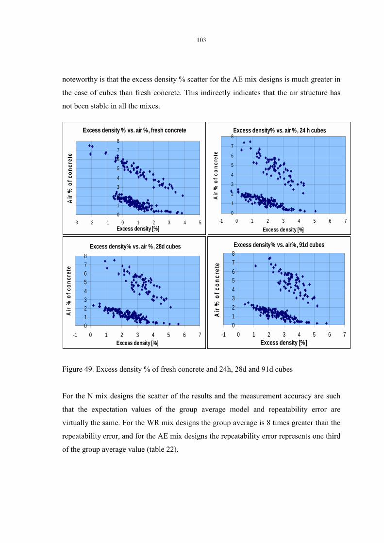
103
noteworthy is that the excess density % scatter for the AE mix designs is much greater in
the case of cubes than fresh concrete. This indirectly indicates that the air structure has
not been stable in all the mixes.
Figure 49. Excess density % of fresh concrete and 24h, 28d and 91d cubes
For the N mix designs the scatter of the results and the measurement accuracy are such
that the expectation values of the group average model and repeatability error are
virtually the same. For the WR mix designs the group average is 8 times greater than the
repeatability error, and for the AE mix designs the repeatability error represents one third
of the group average value (table 22).
Excess density % vs. air %, fresh concrete
0
1
2
3
4
5
6
7
8
-3 -2 -1 0 1 2 3 4 5Excess density [%]
Air
% o
f co
ncre
te
Excess density% vs. air %, 24 h cubes
0
1
2
3
4
5
6
7
8
-1 0 1 2 3 4 5 6 7
Excess density [%]
Air
% o
f co
ncr
ete
Excess density% vs. air %, 28d cubes
012345678
-1 0 1 2 3 4 5 6 7Excess density [%]
Air
% o
f con
cret
e
Excess density% vs. air%, 91d cubes
012345678
-1 0 1 2 3 4 5 6 7Excess density [%]
Air
% o
f co
ncr
ete

104
Table 22. Air % repeatability error and group average
median of 90% quantile (10%-90% quantiles for the median)
N WR AE All
Repeatability error[%] 0.3
(0.2�0.4)
0.1
(0.1-0.2)
0.4
(0.3-0.8)
0.3
(0.2-0.3)
Group Average [%] 0.4
(0.4-0.5)
0.8
(0.6-0.8)
1.5
(1.1-2.2)
0.9
(0.8-1.0)
For the N and WR mix designs, a strong inverse correlation, R = -0.91, between the
entrapped air and flow value can be detected, i.e. when the workability is poor, the
normal compaction energy is not sufficient to force the air out of the concrete (figure 50).
The reverse phenomenon applies to the AE mix designs, R = 0.89 and R = 0.52 for the
AE30 and AE35 respectively. When the workability is good, the entrained air % also
tends to be higher (figure 50).
Figure 50. Correlation between entrapped and entrained air % and flow values
As the correlations are so strong, we can conclude that fine aggregate characteristics that
affect the workability also affect the entrapped air %. When the amount of paste is low,
the entrained air % is also influenced by aggregate characteristics that affect the
workability. With higher amounts of paste, other mix design and/or aggregate
characteristics begin to compensate for the influence.
Air % (N & WR) vs. Flow 5 min
R = -0.91
250
450
650
850
0 0.5 1 1.5 2 2.5 3
Air %, fresh concrete
Flo
w [m
m]
Air % (AE) vs. Flow 5 min
R = 0.89
R = 0.52
250
350
450
550
0 2 4 6 8
Air %, fresh concrete
Flo
w [
mm
]
AE30
AE35

105
6.2.2 Air %, hardened concrete
Thin sections of all the AE castings were made for air analysis. The factors determined
were: the entrained and entrapped air %, the specific surface of the entrained air voids,
and the spacing factor, i.e. the thickness of the hardened cement paste between adjacent
air voids. Tables 23 and 24 present the thin-section statistics for the AE30 and AE35 mix
designs. Additionally, for comparison purposes, the tables show the air % statistics, with
the volumetric method from the fresh concrete.
Table 23. Thin-section statistics from the AE30 mix design
Table 24. Thin-section statistics from the AE35 mix design
As can be seen from tables 23 and 24, the AE30 castings are more homogenous with the
air quality. Furthermore, the deviations between the volumetric air % and thin-section air
% are smaller for the AE30 than for the AE35 castings.
These results reveal that the repeatability of the thin-section is two sided. The results
were relatively constant if the air void system was stable and if not, they could deviate
strongly from each other (table 25 and figures 51). The repeatability error for the
volumetric method is covered in chapter 6.2.
AE30
Entrained air
[%]
Entrapped air
[%]
Total air [%] Specific surface of
voids [mm2]
Spacing
Factor
Volumetric
method
AE30
Total air [%]
avg 2.6 1.5 4.1 44 0.16 avg 3.9stdev 1.0 0.9 1.3 10 0.05 stdev 0.9max 6.4 4.1 7.2 67 0.29 max 6.6min 1.1 0.2 2.5 27 0.10 min 2.1
AE35
Entrained air
[%]
Entrapped air
[%]
Total air [%] Specific surface of
voids [mm2]
Spacing
Factor
Volumetric
method
AE35
Total air [%]avg 3.2 1.5 4.7 42 0.20 avg 5.4
stdev 1.3 1.1 1.8 11 0.20 stdev 0.9max 5.7 3.6 8.1 60 1.07 max 7.5min 0.3 0.0 0.6 15 0.11 min 3.0

106
Table 25. Examples of thin-section analysis results from repeated castings
Casting # 64 Casting # 58
Figure 51. Pictures of repetition castings of the same mix with unstable
void structure.
The castings had very similar fresh concrete values;
air 6.0% and 5.6%, flow value 440 mm and 435 mm,
bleeding 60 min 1.0 g/cm3 and 1.1 g/cm3
for castings #58 and #64 respectively.
Recipe #Entrained air
[%]
Entrapped air
[%]
Total air [%] Specific surface of
voids [mm2]
Spacing
Factor
AE35: B9 (50%)+ A3 (50%) / B7 (50%) + A2 (50%)26 4.3 0.7 5.0 43 0.1160 3.8 0.2 4.0 47 0.1166 4.5 0.2 4.7 35 0.1489 3.5 2.1 5.6 46 0.12140 3.0 1.5 4.5 58 0.11
AE35: B7 (100%) / B7 (100%)58 0.5 3 3.5 15 0.8564 4.3 3.2 7.5 43 0.13

107
6.3 Bleeding
The bleeding was determined at three time intervals: 10, 30, 60 minutes after the mixing
was completed. Normally the bleeding proceeds at a constant rate, and water appears on
the surface as the mix constituents settle downwards. However, if the concrete
segregates, the water comes to the surface directly after mixing. These phenomena can be
seen from tables 26 and 27 and figure 52, which present the 10 min, 30 min and 60 min
bleeding statistics for the six mix designs. Table 28 shows the bleeding 60 min
repeatability error and group average confidence limits with quantiles for the N, WR and
AE mix designs.
Table 26. Bleeding 10 minutes, statistics for each mix design
10 min [g/cm3] N30 N35 WR30 WR35 AE30 AE35 All
Average 0.0 0.0 0.0 1.2 0.0 0.0 0.4
Stdev 0.1 0.1 0.0 3.0 0.0 0.4 2.7
Max 0.3 0.3 0.0 13.6 0.0 1.0 25.5
Min 0.0 0.0 0.0 0.0 0.0 0.0 0.0
Table 27. Bleeding 30 minutes, statistics for each mix design
30 min [g/cm3] N30 N35 WR30 WR35 AE30 AE35 All
Average 1.1 1.8 0.1 2.3 0.3 0.4 1.4
Stdev 0.6 0.8 0.3 3.8 0.3 0.2 4.4
Max 2.9 4.2 1.5 13.3 0.9 1.0 44.1
Min 0.0 0.2 0.0 0.0 0.0 0.0 0.2
Table 28. Bleeding test repeatability error and group average
median of 90% quantile (10%-90% quantiles for the median)
N WR AE All
Repeatability error [g/cm3] 1.1
(0.8-3.2)
2.2
(1.5-4.0)
0.3
(0.2-0.6)
1.3
(1.1-1.7)
Group Average [g/cm3] 2.5
(2.3-3.2)
3.6
(2.2-7.8)
0.9
(0.6-1.2)
2.3
(2.0-2.5)

108
Though the expectation values of the repeatability errors are smaller than the group
average, the quantiles for the repeatability median are large, and thus the measurement
error can actually even exceed the bleeding estimation based on the group average (N
and WR mix designs). The determination of what was bleeding water and what was grout
(cement+water) from the segregated castings was difficult and has thus increased the
repeatability error. Results for two castings were even disregarded for this reason (values
for bleeding 60 min; 47.9 and 58.2 g/cm3).
Figure 52. Bleeding 60 min statistics for each mix design
Both the air-entraining agent and superplasticizer decrease bleeding in comparison with
no-admixture concrete. An exception occurs when the superplasticizer is used with
concrete of very high workability. In this case, the bleeding increased substantially due to
the segregation (figure 53). This phenomenon involved some WR35 castings, where the
water absorption characteristics of the aggregate composition, the particle porosity of the
SCF and the BET value of the fines were small/low. As can be seen, the correlation is
significant for all mix designs but is highest for the WR35 mix design.
Bleeding 60 min
1.3=s tde v
1.8 0.5 4.8 0.5 0.6 2.6
0
4
8
12
16
20
Ble
edin
g [
g/c
m3 ]
avg [g /cm 3] 3.2 4.9 0.6 7.6 1.1 1.5 2.6
m ax 6.8 9.6 2.5 18.5 2.6 3.0 18.5
m in 0.8 0.9 0.1 0.3 0.4 0.2 0.1
N30 N35 WR30 WR35 AE30 AE35 All

109
Figure 53. Correlation between flow value and bleeding
The dividing line between the bleeding and segregation is blurred, and what is typical of
bleeding is that when the threshold for the ability to hold the mixing water is passed the
bleeding tendency increases rapidly. This can be observed from figures 54 and 55, which
show the correlations between F-BET value and bleeding for the N30 mix design, and
between SC- pore area >900Å and bleeding for the AE30 mix design.
Figure 54. Correlation between F- BET value and bleeding; N30
Figure 55. Correlation between SC- pore area >900Å and bleeding; AE30
BET (N30) vs. Bleeding 60 min
R = -0.60
0
2
4
6
8
0 5 10 15
BET value [m2/g]
Ble
edin
g [
g/c
m3 ]
Pore area S-C, >0.09 µm, (AE30) vs. Bleeding 60 min
R = -0.77
0
1
2
3
0 0.05 0.1 0.15
Pore Area >0.09 µm [m2/g]
Ble
edin
g [
g/c
m3 ]
Flow value (WR35) vs. Bleeding 60 min
R = 0.80
0
4
8
12
16
20
500 550 600 650 700 750
Flow value [mm]
Ble
edin
g [
g/c
m3]
N30 0.46N35 0.58
WR30 0.44WR35 0.80AE30 0.44AE35 0.38
Correlation for each mix design

110
Both the F- BET value and the SC- pore area are characteristics that describe the
absorption tendencies and also the water-retaining capacity of the aggregate. If the
aggregate combination has a low value for both these aspects, bleeding will occur. The
amount is dependent on the mix design and admixture combination.
6.4 Compressive strength
The compressive strength was determined at three ages, 1d, 28d and 91d. For each
casting and age, the compressive strength was calculated as an average of three parallel
cubes. Tables 29, 30 and figure 56 present the mix design average, standard deviation,
maximum value and minimum value for 1d, 28 d and 91d respectively for the six mix
designs. The standard deviation results, 1d, 28d and 91d, for the three parallel cubes is
presented in table 31.
Table 29. Compressive strength statistics for each mix design, 1d
1d [MPa] N30 N35 WR30 WR35 AE30 AE35 All
Average 15.0 14.4 20.9 20.0 17.7 15.7 17.1
Stdev 1.2 0.9 1.5 1.4 1.9 1.3 2.9
Max 18.0 16.3 24.3 23.5 20.7 19.3 24.3
Min 12.2 12.0 18.3 17.1 13.6 12.6 12.0
Table 30. Compressive strength statistics for each mix design, 28d
28d [MPa] N30 N35 WR30 WR35 AE30 AE35 All
Average 42.6 42.3 52.0 51.3 43.0 39.5 44.9
Stdev 3.0 2.0 4.5 2.9 2.7 2.5 5.7
Max 46.6 45.4 57.6 54.5 48.1 46.2 57.6
Min 34.6 36.8 40.4 42.5 37.6 34.5 34.5

111
Table 31. Standard deviation statistics for the three parallel cubes
C stdev [MPa] 1d 28d 91d
Average stdev 0.3 0.6 0.7
Stdev 0.1 0.3 0.3
Max 0.9 1.4 1.5
Min 0.0 0.1 0.1
Figure 56. Compressive strength statistics for each mix design, 91 d
The basis for the mix designs was two fixed amounts of cement, 300 kg/m3 and 350
kg/m3, and the same starting workability with one fines/semi-coarse aggregate
combination. This led to different w/c ratios and thus variable compressive strength
levels with different mix designs. However, within a mix design group the compressive
strength should be the same, because the w/c ratio was constant for the two amounts of
cement. At all ages, the WR mix designs have the highest compressive strength (w/c =
0.58) and the N and AE mix designs have approximately 20% lower values at each age
(w/c = 0.65 and 0.58 respectively). The AE30 mix design has higher compressive
strength than the AE35 mix design, because the air % attained is lower, and the strength
Compressive Strength, 91d
6.32.72.93.05.12.12.8=stdev
35
40
45
50
55
60
65
Co
mp
. str
eng
th [
MP
a]
avg [MPa] 47.8 47.2 58.2 57.7 47.8 44.1 50.2
m ax 51.7 51.7 64.0 60.8 52.4 50.3 64.0
m in 37.7 43.3 45.2 46.6 39.8 37.6 37.6
N30 N35 WR30 WR35 AE30 AE35 All

112
is thus reduced less. The average standard deviation for the three parallel compressive
strength cubes is half of the repeatability error between the repetition castings (table 32
and 31).
Table 32. Compressive strength repeatability error and group average
median of 90% quantile (10%-90% quantiles for the median)
N WR AE All
Repeatability error [MPa] 2.2
(1.6-3.3)
2.5
(1.8-3.9)
1.6
(1.0-3.1)
2.1
(1.8-2.7)
Group Average [MPa] 4.3
(3.4-4.8)
9.3
(4.6-12.4)
4.9
(4.1-6.3)
4.8
(4.6-5.6)
For the N mix designs the repeatability error is approximately 50% of the group average,
and for the WR and AE mix designs the group average exceeds the repeatability error by
over 300%.
The air % has a strong influence on the achievable compressive strength. Figure 57a
shows the correlation for the WR mix designs (R = -0.73 for the WR30 and R = -0.53 for
the WR35), and figure 57b presents the correlation for the AE mix designs (R = -0.73).
The corresponding values for the N30 and N35 mix designs are R = -0.56 and R = -0.39
respectively.
Figure 57. Correlation between air % and compressive strength
Air % (AE) vs. Compressive Strenght 91d
R = -0.73
30
35
40
45
50
55
0 2 4 6 8
Air %, fresh concrete
Co
pm
ress
ive
Str
eng
ht [
MP
a]
Air % (WR) vs. Compressive Strength 91d
R = -0.73
R = -0.53
45
50
55
60
65
0 1 2 3
Air %, fresh concrete
Co
mp
ress
ive
Str
eng
th [
MP
a]
WR35
WR30

113
Other characteristics that have a strong influence and which can be seen from the linear
correlation calculations are the SC- Los Angeles value and SC- quantity of the particles.
Figure 58a presents the correlation between the SC- LA value (mod.) and compressive
strength at 91d for the WR mix designs. Figure 58b shows the correlation between SC-
particle quantity 3.15/4.0 mm and compressive strength for the N mix designs. The
correlation between the SC- quantity of the particles and the SC- LA value is R = 0.66.
Figure 58a. Correlation between SC- Los Angeles (mod.) value and
compressive strength at 91d, WR mix designs
Figure 58b. Correlation between SC- quantity 3.15/4.0 mm and
compressive strength at 91d, N mix designs
As can be seen, the effect of the SC- LA value and the SC-quantity can be is as high as
15…25 % of the absolute value of the compressive strength. The correlations with the
other mix designs are also significant, except in the case of AE30.
Los Angeles (mod.) -value (WR) vs. Compressive Strength 91d
R = -0.90
R = -0.85
40
50
60
70
20 25 30 35 40
Los Angeles (mod.) [%]
Co
mp
. Str
eng
th [
MP
a]
WR30
WR35
Quantity 3.15/4.0 mm (N) vs.Compressive Strength 91d
R = -0.82
R = -0.66
35
40
45
50
55
3.E+06 3.E+06 4.E+06 4.E+06 5.E+06
Quantity 3.15/4.0 mm
Com
p. S
tren
gth
[MP
a]
N30
N35

114
6.5 Drying shrinkage and weight change
6.5.1 Results
The shrinkage and weight measurements were conducted 10 to 13 times during the 231d
period during which the prisms were observed. For each casting, the results are
calculated as an average of two parallel prisms. The standard deviation statistics for the
231d results for two parallel prisms is presented in table 33. The repeatability errors for
the drying shrinkage and weight change are 0.060 ± 0.012 o/oo and 0.088 ± 0.020 %
respectively.
Table 33. Standard deviation statistics for the drying shrinkage and
weight change, two parallel prisms, 231d
[ o/oo ] Drying shrinkage Weight change [ % ]
Average stdev 0.011 0.054 Average stdev
Stdev 0.009 0.045 Stdev
Max 0.037 0.192 Max
Min 0.000 0.001 Min
Figures 59 and 60 show the average, standard deviation, maximum and minimum values
for the 231d drying shrinkage and weight change for three mix designs. The number of
castings per mix design was 15, 16 and 16 castings for N35, WR30 and AE35
respectively.
Figures 61 and 62 show the drying shrinkage and weight change development for
particular fines/semi-coarse combinations (7 castings) to verify the variations between
and within the mix designs.

115
Figures 59 and 60. Drying shrinkage and weight change statistics, 231d
Figures 61 and 62. Drying shrinkage and weight change due to the mix design variation
As can be seen from the results, the variation in drying shrinkage within a mix design is
greater than the variation between them. The maximum difference between the mix
designs is 20 % (WR30 – AE35), while the difference between max-min values within a
mix design is 43%, 39% and 28% for the N35, WR30 and AE35 respectively. This
indicates that the effect of the fine aggregate characteristics exceeds the effect of the mix
design.
Drying Shrinkage, 231d
0.0740.0540.0550.069 =stdev
0.5
0.6
0.7
0.8
0.9
Sh
rin
kag
e [o
/oo
]
avg [o/oo] 0.641 0.564 0.670 0.625
max 0.797 0.702 0.749 0.797
min 0.555 0.505 0.583 0.505
N35 WR30 AE35 All
Weight Change, 231d
0.4800.1320.1280.138=stdev
-3.0
-2.5
-2.0
-1.5
-1.0
Wei
gh
t ch
ang
e [%
]
avg [%] -2.566 -1.438 -2.009 -1.992
max -2.362 -1.181 -1.826 -1.181
min -2.884 -1.630 -2.242 -2.884
N35 WR30 AE35 All
Drying Shrinkage AVG (B1/B1, A8/A8, A16/A16, B11/B11, B2/B2, B13/B13, B8/B8)
-0.1
0.0
0.1
0.2
0.3
0.4
0.5
0.6
0.7
0 50 100 150 200 250
Age [d]
Sh
rin
kag
e [o
/oo
]
N35
AE35
WR30
Weight ChangeAVG (B1/B1, A8/A8, A16/A16, B11/B11, B2/B2, B13/B13, B8/B8)
-3
-2.5
-2
-1.5
-1
-0.5
0
0.5
1
0 50 100 150 200 250
Age [d]
Wei
gh
t ch
ang
e [%
]
N35
AE35
WR30

116
The weight change is more strongly affected by the mix design than by the aggregate
characteristics. The variation between the mix designs is nearly 80 % (N35 – WR30),
while the variations within the mix designs are only 22%, 38% and 23% for the N35,
WR30 and AE35 respectively. If we calculate the weight change relative to the total
water amount, and compare the results to the weight change of the N35 mix design, we
observe that the weight changes of the WR30 and AE35 mix designs are 54% and 75%
respectively.
If the results are analysed from the point of view of aggregate products, we obtain
figures, which reveal the dominating aggregate characteristics. Figures 63 and 64 present
the drying shrinkage and weight change curves for the same 7 castings in such a way that
the curve represents the average of the three mix designs (N35, WR30, AE35) for each
aggregate combination.
Figure 63. Drying shrinkage scatter due to aggregate characteristics
Drying Shrinkage, AVG (N35,AE35, WR30)
-0.1
0.0
0.1
0.2
0.3
0.4
0.5
0.6
0.7
0.8
0 50 100 150 200 250
Age [d]
Shrinka
ge
[o/o
o]
B1/B1
A8/A8
A16/A16
B11/B11
B2/B2
B13/B13
B8/B8

117
Figure 64. Weight change scatter due to aggregate characteristics
The largest shrinkage occurs in the case of the aggregate combinations B8/B8, B11/B11
and B1/B1, which all have a high SCF particle porosity and fines surface area (figure 30
and 32 chapter 5). A8/A8 and A16/A16 are both castings with only rock aggregate
products and do not have excessively high SCF particle porosity characteristics. A8
represents a poor particle shape and thus has a high quantity of particles, whereas A16
has a fair particle shape, which results in fewer particles as compared to the A8. Hence,
the shape quality of particles does not seem to affect the drying shrinkage if the loss of
workability is accepted and thus, the paste amount is kept constant.
The difference between the highest and lowest weight changes is not especially large, nor
can any aggregate quality characteristics particularly be related to the weight changes.
Figure 65 shows how much the shrinkage properties can be affected merely by a change
in the fines (<0.125 mm).
Weight Change, AVG (N35,AE35, WR30)
-2.5
-2
-1.5
-1
-0.5
0
0.5
1
0 50 100 150 200 250
Age [d]
Wei
gh
t ch
ang
e [%
]
B1/B1
A8/A8
A16/A16
B11/B11
B2/B2
B13/B13
B8/B8

118
Figure 65. Effect of the fines, < 0.125 mm on drying shrinkage
Even the B1 and B3 represent very different fines quality, the amount of fines in the
combined grading curve is only 3…4%, yet the effect on the shrinkage is approximately
5% (231d). The repeatability error is greater than the observed fine fraction effect, but as
the difference is calculated as an average of three mix designs, the phenomenon is
statistically valid.
6.5.2 Discussion
The weathering properties of the gravel aggregate increase the shrinkage. In the case of
weathered aggregates, the drying shrinkage is partly self-induced, as the water absorption
reduces the workability, extra water is needed for replacement; together with the time-
dependent water evaporation from the aggregate pores, this in turn further increase the
shrinkage. In the case of the present test programme, the effect of the aggregate
D rying Shrinkage - Effect of the fines AVG (N35, AE35, WR 30)
-0.1
0.0
0.1
0.2
0.3
0.4
0.5
0.6
0.7
0.8
0 50 100 150 200 250
Age [d]
Sh
rin
kag
e o
/oo
B3/B1
B1/B1

119
characteristics on the drying shrinkage was more than twice as large as the effect of
changes in the mix design.
For drying shrinkage purposes, the best information on the potential shrinkage is
obtained if the water/cement ratio of the mix design is expressed by means of the total
water content instead of the effective amount of water. As the rock aggregate products
are not normally weathered, the shrinkage potential is thus lower than in the case of
normal gravel aggregates, but the possible extra water and/or paste needed for good
workability increases the tendency. However, the results of this study make it possible to
assume that even though corrective changes in the mix design were made, the shrinkage
increase is less that the effect of moderately weathered gravel aggregate. Consequently, if
a non-weathered gravel aggregate product is available, both the drying shrinkage and the
w/c ratio for good workability are low.
By means of aggregate production technology, it is possible to reduce the effect that the
fine aggregate has on the drying shrinkage. If the gravel fine aggregate is weathered, it is
possible to reduce the effect by using, for example, the following aggregate production
techniques:
• Crushing the gravel (totally or partly), because in this case fresh, unweathered
surfaces open
• Sieving off (dry or wet sieving) the finest fractions, because they have the largest
surface area and thus particle porosity and replacing them with unweathered filler
aggregate
It should, however, be remembered, that the fines are derived from the semi-coarse
particles and that the same characteristics are thus valid for all size fractions. Therefore,
if it is not possible to exclude a phenomenon, the effect and its magnitude should be
known and altered within the possible limits.

120
7 MODELS FOR THE FINE AGGREGATE – CONCRETE INTERACTION
7.1 Model for the flow value
The model for the flow value consists of 12 parameters: 3 mix design characteristics and
5 semi-coarse and 4 fines characteristics. Figure 66 shows the ARD listing for the
parameters.
Figure 66. ARD listing of the parameters for the modelled flow value
Asterisk =mean value; diamond =median value;
box = 25-75 % quantiles; line = 10-90 % quantiles
The median of the 90% quantile and its 10% and 90% quantiles for the model error are
presented in table 34.
Cu
Mica% fines
Pore area > 900 Å
Elgn 3.15/4.0 mm
Angularity
AE
Pore area 300-900 Å
Flkn 3.15/4.0 mm
WR
SEM
ZETA pot.
BET
-4 -3 -2 -1 0

121
Table 34. Flow group averages and repeatability and model errors
median of 90% quantile (10%-90% quantiles for 90% quantile)
N WR AE All
Repeatability error[mm] 21
(16-31)
9
(6-13)
10
(6-19)
15
(13-19)
Group Average [mm] 70
(62-89)
128
(122-139)
61
(48-72)
104
(97-119)
Model error [mm] 34
(32-41)
39
(33-47)
30
(26-34)
34
(32-38)
For the N and AE mix designs the model is 50% more accurate than the group average,
and for the WR mix designs the value is as high as 70%. The repeatability errors
represent 23% to 62% of the different mix design model errors and 44% of the model
error for all the mix designs. One workability class is 60 mm (EN206) and as the model
error is 34 mm (32-38), the model error constitutes approximately half a workability
class. Consequently, the repeatability error is a quarter of a workability class.
Figure 67 shows correlation plots for measured vs. modelled flow value for the AE mix
designs and the N&WR mix designs. Table 35 presents the correlations for each mix
design, for mix design groups and for all mix designs.
Figure 67. Correlation plots for measured vs. modelled flow value
AE mix designs and N & WR mix designs
Measured vs. modelled FLOW value, AE mix designs
R = 0.99
250
350
450
550
250 300 350 400 450 500 550
Measured flow value [mm]
Mod
elle
d fl
ow v
alue
[m
m]
Measured vs. modelled FLOW value, N & WR mix designs
R = 0.99
250
350
450
550
650
750
250 350 450 550 650 750
Measured flow value [mm]
Mod
elle
d fl
ow v
alue
[m
m]

122
Table 35. Correlations between measured and modelled flow value for
each mix design, mix design groups and all mix designs
7.1.1 Sensitivity analysis – flow value
7.1.1.1 Reliability of the sensitivity analysis – flow value
The reliability figures for the flow value sensitivity analyses are presented in appendix 4.
As can be seen from the figures, the deviations between the measured and the modelled
values in general constitute less than half a workability class. Greater differences are
mainly concentrated among the N30 castings.
7.1.1.2 Flow value – SC- flakiness 3.15/4.0 mm, SC- angularity and
SC- elongation 3.15/4.0 mm
The flakiness 3.15/4.0 mm has a strong effect on workability in all mix designs (figure
68). The effect is also approximately the same for all mix designs.
The angularity affects the workability of the WR mix designs most strongly. To some
extent, it also influences the N30 and AE30 mix designs, but the effect seems to be
negligible on the higher paste amount mix designs containing a higher amount of paste,
i.e. N35 and AE35 (figure 69).
The effect of the elongation 3.15/4.0 mm is not linear. In the case of the lower elongation
values, there is a negative effect on workability, but after certain limit, the increase in
elongation enhances workability (figure 70). However, the enhancing effect is dependent
on the amount of paste, so that this effect is stronger for mix designs with a higher paste
amount, i.e. N35, WR35 and AE35.
AE30 AE35 N30 N35 WR30 WR35 WR N N&WR AE ALL0.97 0.94 0.97 0.97 0.99 0.99 1.00 0.98 0.99 0.99 0.99

123
Figure 68. Sensitivity analysis figure; SC- flakiness 3.15/4.0–flow value
Figure 69. Sensitivity analysis–figure; SC- angularity–flow value
Sensitivity analysis
0
100
200
300
400
500
600
700
800
1.2 1.25 1.3 1.35 1.4 1.45
SC-Flkn 3.15/4.0 mm
Flo
w v
alu
e [m
m]
N30
WR30AE30
N35WR35
AE35
Sensitivity analysis
0
100
200
300
400
500
600
700
800
4.5 5 5.5 6 6.5 7 7.5 8 8.5 9
SC-Angularity
Flo
w v
alu
e [m
m]
N30W R30AE30N35W R35AE35

124
Figure 70. Sensitivity analysis figure; SC-elongation 3.15/4.0 mm–flow value
7.1.1.3 Flow value – SC- pore area 300-900 Å and SC- pore area > 900 Å
Both the SC- pore area values have significant effect on the flow value, (figures 71 and
72).
Figure 71. Sensitivity analysis figure; SC- pore area 300-900Å–flow value
Sensitivity analysis
0
100
200
300
400
500
600
700
800
1.34 1.36 1.38 1.4 1.42 1.44 1.46 1.48
SC-Elgn 3.15/4.0 mm
Flo
w v
alu
e [m
m]
N30W R30AE30N35W R35AE35
Sensitivity analysis
0
100
200
300
400
500
600
700
800
0 0.02 0.04 0.06 0.08 0.1 0.12 0.14
SC-pore area 300-900Å [m2/g]
Flo
w v
alu
e [m
m]
N30W R30AE30N35W R35AE35

125
Figure 72. Sensitivity analysis figure; SC- pore area > 900Å–flow value
7.1.1.4 Flow value – >F- Mica %, F- Cu, F- BET value and F- zeta potential
The effect of the percentage of F- mica % fines alone seems to be negligible (figure 73),
and thus can be assumed that it acts in combination with other fines inputs. The situation
is the same in the case of F- zeta potential (figure 74).
The sensitivity analysis for F- Cu, figure 75, shows a slight general negative effect on
workability accompanying an increased F- Cu value. The effect is approximately equal
for all mix designs.
An increase in the F- BET value also has a negative effect on workability. However,
different behaviour is seen with different mix designs; the effect on mix designs
containing superplasticizer is the strongest (figure 76).
Sensitivity analysis
0
100
200
300
400
500
600
700
800
0 0.02 0.04 0.06 0.08 0.1 0.12 0.14
SC-pore area>900Å [m2/g]
Flo
w v
alu
e [m
m]
N30W R30AE30N35W R35AE35

126
Figure 73. Sensitivity analysis figure; %F- mica fines–flow value
Figure 75. Sensitivity analysis figure; F- Cu–flow value
Sensitivity analysis
0
100
200
300
400
500
600
700
800
0 2 4 6 8 10 12 14 16
F - mica %
Flo
w v
alu
e [m
m]
N30WR30AE30N35WR35AE35
Sensitivity analysis
0
100
200
300
400
500
600
700
800
0 2 4 6 8 10 12 14 16 18
F - Cu
Flo
w v
alu
e [m
m]
N30WR30
AE30
N35WR35
AE35

127
Figure 76. Sensitivity analysis figure; F- BET value–flow value
Figure 74. Sensitivity analysis figure; F- Zeta potential–flow value
Sensitivity analysis
0
100
200
300
400
500
600
700
800
0 2 4 6 8 10 12 14 16
F- BET [m2/g]
Flo
w v
alu
e [m
m]
N30WR30
AE30
N35WR35
AE35
Sensitivity analysis
0
100
200
300
400
500
600
700
800
-20 -18 -16 -14 -12 -10 -8 -6 -4 -2 0
F - Zeta pot. [mV]
Flo
w v
alu
e [m
m]
N30WR30
AE30
N35WR35
AE35

128
7.2 Model for air %, fresh concrete
The model for the air % in fresh concrete consists of 9 parameters: 3 mix design
characteristics and 4 are semi-coarse and 2 fines characteristics. Figure 77 shows the
ARD listing for the parameters.
Figure 77. ARD listing of the parameters for the modelled air %
Asterisk = mean value; diamond = median value;
box = 25-75 % quantiles; line = 10-90 % quantiles
The median of the 90% quantile and its 10% and 90% quantiles for the model error are
presented in table 36.
Table 36 Air % group averages and repeatability and model errors
median of 90% quantile (10%-90% quantiles for 90% quantile)N WR AE All
Repeatability error[%] 0.3(0.2–0.4)
0.1(0.1-0.2)
0.4(0.3-0.8)
0.3(0.2-0.3)
Group Average [%] 0.4(0.4-0.5)
0.8(0.6-0.8)
1.5(1.1-2.2)
0.9(0.8-1.0)
Model error [%] 0.2(0.2-0.3)
0.4(0.3-0.5)
0.9(0.8-1.1)
0.6(0.5-0.7)
Flk 3.15/4.0mm
Pore area 300-900Å
Angularity
WR
SEM
Pore area 60-300Å
AE
Cu
BET
-4 -3 -2 -1 0 1 2 3

129
When one compares the model errors to the group averages, the explication is enhanced
approximately 50 %. For all the mix designs the model error is twice the repeatability
error and 65 % of the group average model.
Figure 78 presents correlation plots for measured vs. modelled air % for the AE mix
designs and the N&WR mix designs. Table 37 below further presents the correlations for
each mix design, for mix design groups and for all mix designs.
Figure 78. Correlation plots for measured air % vs. modelled air %
Table 37. Correlations between measured air % and modelled air % for each mix
design, mix design group and all mix designs
7.2.1 Sensitivity analysis – air %
7.2.1.1 Reliability of the sensitivity analysis – air %
The reliability figures for the air % sensitivity analyses are presented in appendix 4. For
the N and WR mix designs the deviations between the modelled and measured values is
clearly less than 0.5%-unit. Generally this is also the case for the AE mix designs, though
there are several castings where the deviation is as high as 1.5%-unit.
Measured vs. modelled AIR %, N & WR mix designs
R = 0.98
0
1
2
3
0 1 2 3
Measured air %
Mo
del
led
air
%
Measured vs. modelled AIR %, AE mix designs
R = 0.95
2
4
6
8
2 3 4 5 6 7 8
Measured air %
Mo
del
led
air
%
AE30 AE35 N30 N35 WR30 WR35 WR N N&WR AE ALL0.92 0.91 0.9 0.96 0.95 0.95 0.98 0.97 0.98 0.95 0.99

130
7.2.1.2 Air % - SC- pore area 60-300Å and SC- pore area 300-900Å
The SC- pore area 60-300Å and 300-900Å have a similar effect on the mix designs, i.e.
the air % increases with the N and WR mix designs and decreases with the AE mix
designs (figure 79 and 80).
Figure 79. Sensitivity analysis figure; SC- pore area 60-300 Å–air %
At low amount of pore area the shape characteristics act together, causing the air % to
increase in the case of the AE30 and decrease in that of the N and WR mix designs.
Additionally noteworthy for both SC- pore area inputs is the fact that the decrease in the
air % is very dramatic in the range of medium-amount of the pore area, but seems to
recover at the higher-amount of pore area. This phenomenon is most likely due to
different aggregate products and thus difference in the pore structure. The measurements
were though conducted similarly for all aggregate products.
Sensitivity analysis
0
1
2
3
4
5
6
7
8
-0.02 0 0.02 0.04 0.06 0.08 0.1 0.12 0.14 0.16
SC-pore area 60-300Å [m2/g]
Air
%
N30WR30
AE30
N35WR35
AE35

131
Figure 80. Sensitivity analysis figure; SC- pore area 300-900 Å–air %
7.2.1.3 Air % - SC- flakiness 3.15/4.0 mm and SC-angularity
When the SC- flakiness 3.15/4.0 mm increases, the effect of it on the two AE mix
designs is the opposite: the air % of the AE30 mix design decreases and the air % of the
AE35 mix design increases, to an even greater extent. The effect on the N and WR mix
designs is negligible (figure 81).
SC- angularity has a decreasing effect on the air % of the AE mix designs. The effect is
stronger in the case of the AE35. For the N and WR mix designs, SC- angularity has a
slight effect on the entrapped air % (figure 82).
Sensitivity analysis
0
1
2
3
4
5
6
7
8
-0.02 0 0.02 0.04 0.06 0.08 0.1 0.12 0.14
SC-pore area 300-900Å [m2/g]
Air
%
N30WR30
AE30
N35WR35
AE35

132
Figure 81. Sensitivity analysis figure; SC- flakiness 3.15/4.0 mm–air %
Figure 82. Sensitivity analysis figure; SC- angularity–air %
Sensitivity analysis
0
1
2
3
4
5
6
7
8
1.2 1.25 1.3 1.35 1.4 1.45
SC-Flkn 3.15/4.0 mm
Air
%
N30WR30
AE30
N35WR35
AE35
Sensitivity analysis
0
1
2
3
4
5
6
7
8
4.5 5 5.5 6 6.5 7 7.5 8 8.5 9
SC-Angularity
Air
%
N30WR30
AE30
N35WR35
AE35

133
7.2.1.4 Air % - F- Cu and F- BET value
The effects of the F- Cu and F- BET value are not very strong, and for the N and WR mix
designs the influence is almost negligible (figures 83 and 84). When the F- Cu increases
the air % decreases and the influence is slightly stronger on the AE30 mix design. An
increase in the F- BET value also decreases the air % and seems to influence the AE35
mix design somewhat more strongly.
Figure 83. Sensitivity analysis figure; F- Cu–air %
Figure 84. Sensitivity analysis figure; F- BET value–air %
Sensitivity analysis
0
1
2
3
4
5
6
7
8
2 4 6 8 10 12 14 16 18
F - Cu
Air
%
N30WR30
AE30
N35WR35
AE35
Sensitivity analysis
0
1
2
3
4
5
6
7
8
0 2 4 6 8 10 12 14 16
F- BET [m2/g]
Air
%
N30
WR30
AE30N35
WR35AE35

134
7.3 Model for the bleeding
The model for the bleeding 60 min consists of 12 parameters, 3 mix design
characteristics and 5 semi-coarse and 4 fines characteristics. The figure 85 shows the
ARD listing for the parameters. The median of the 90% quantile and its 10% and 90%
quantiles for the model error are presented in table 38.
Figure 85. ARD listing of the parameters for the modelled bleeding
Asterisk = mean value; diamond = median value;
box = 25-75 % quantiles; line = 10-90 % quantiles
Table 38. Bleeding group averages and repeatability and model errors
median of 90% quantile (10%-90% quantiles for 90% quantile)N WR AE All
Repeatability error [g/cm3] 1.1(0.8-3.2)
2.2(1.5-4.0)
0.3(0.2-0.6)
1.3(1.1-1.7)
Group Average [g/cm3] 2.5(2.3-3.2)
3.6(2.2-7.8)
0.9(0.6-1.2)
2.3(2.0-2.5)
Model error [g/cm3] 2.2(1.8-2.8)
2.8(1.1-6.3)
0.7(0.4-0.9)
1.8(1.3-2.2)
WR
SEM
Tot. pore area SC
AE
Elgn 0.8/1.0 mm
Flkn 1.6/2.0 mm
BET
Avg pore size SC
Elgn 1.6/2.0 mm
ZETA pot.
Density fines
Cu
-4 -3 -2 -1 0 1 2 3

135
If the expectation values of the group average and model are compared, it will be noticed
that no major improvement has occurred. The most important reason for this is the large
deviation in the measurement, i.e. the considerable repeatability error.
Figure 86 presents correlation plots measured vs. modelled bleeding for the WR and N
mix designs. Additionally, table 39 shows the correlations for each mix design, for mix
design groups and for all mix designs.
Figure 86. Correlation plots for measured vs. modelled bleeding
Table 39. Correlations between measured and modelled bleeding
7.3.1 Sensitivity analysis – bleeding
7.3.1.1 Reliability of the sensitivity analysis - bleeding
The model follows the bleeding of all mix designs except the WR35 well. In this case the
model underestimates the higher bleeding values, and some deviations between the
modelled and measured values amount as much as 4 g/cm3. For the N30, AE30, AE35
and WR30 mix designs, which all exhibited low bleeding, the deviation is generally less
Measured vs. modelled BLEEDING, WR mix designs
R = 0.97
0
4
8
12
16
20
0 5 10 15 20
Measured bleeding [g/cm3]
Mo
del
led
ble
edin
g [
g/c
m3 ]
Measured vs. modelled BLEEDING, N mix designs
R = 0.88
0
2
4
6
8
10
0 2 4 6 8 10
Measured bleeding [g/cm3]
Mo
del
led
ble
edin
g [
g/c
m3 ]
AE30 AE35 N30 N35 WR30 WR35 WR N N&WR AE ALL0.88 0.85 0.81 0.86 0.85 0.96 0.97 0.88 0.95 0.87 0.96

136
than 0.5 g/cm3. For the N35 the highest deviations are 2 g/cm3. The reliability figures for
the bleeding sensitivity analyses are presented in appendix 4.
7.3.1.2 Bleeding – SC- total pore area and SC- average pore area
The SC- total pore area has an inhibiting effect on bleeding, and the effect is strongest on
the WR35 mix design (figure 87). Here we can also see the effect of different aggregate
products, i.e. bleeding seems to increase when the SC- total pore area increases (compare
air % model).
Figure 88 shows an extreme case in which the aggregate products have two strong inputs
whose effect works in opposite directions (amount of pore area >< shape) in the case of
the WR35 mix designs. Depending on the value of SC- average pore size, the net effect
on bleeding can be either inhibiting or promoting. For other mix designs, an increase in
the SC- average pore size slightly increases bleeding.
Figure 87. Sensitivity analysis figure; SC- total pore area-bleeding
Sensitivity analysis
0
2
4
6
8
10
12
14
16
18
20
0 0.05 0.1 0.15 0.2 0.25 0.3 0.35 0.4
SC-tot. pore area [m2/g]
Ble
edin
g [
g/c
m3]
N30
WR30
AE30N35
WR35AE35

137
Figure 88. Sensitivity analysis figure; SC- average pore size–bleeding
7.3.1.3 Bleeding–SC- Elongation 0.8/1.0mm, SC- flakiness 1.6/2.0mm and
SC-elongation 1.6/2.0mm
When the elongation 0.8/1.0 mm increases, it increases the bleeding of the WR35 mix
design. In the case of the N35 and WR30, an increase in elongation first increases the
bleeding, though at higher elongation values the bleeding decreases. For other mix
designs the effect is negligible (figure 89).
The flakiness 1.6/2.0 mm decreases bleeding in all the mix designs, but the effect is
strongest in the case of the WR35, N35 and WR30 mix designs (figure 90).
The effect of the elongation 1.6/2.0 mm alone is seemingly negligible in the case of mix
designs other than the WR35 (figure 91).
Sensitivity analysis
0
2
4
6
8
10
12
14
16
18
20
0 2 4 6 8 10 12
SC- avg.pore size [µm]
Ble
edin
g [
g/c
m3]
N30WR30
AE30
N35WR35
AE35

138
Figure 89. Sensitivity analysis figure; SC- elongation 0.8/1.0 mm–bleeding
Figure 90. Sensitivity analysis figure; SC- flakiness 1.6/2.0 mm–bleeding
Sensitivity analysis
0
2
4
6
8
10
12
14
16
1.2 1.25 1.3 1.35 1.4 1.45 1.5
SC-Flkn 1.6/2.0 mm
Ble
edin
g [
g/c
m3]
N30
WR30AE30
N35WR35
AE35
Sensitivity analysis
0
2
4
6
8
10
12
14
16
18
20
1.4 1.45 1.5 1.55 1.6 1.65 1.7
SC-Elgn 0.8/1.0 mm
Ble
edin
g [
g/c
m3]
N30WR30
AE30
N35WR35
AE35

139
Figure 91. Sensitivity analysis figure; SC- elongation 1.6/2.0 mm–bleeding
7.3.1.4 Bleeding – F- BET value, F- zeta potential, F- density and F- Cu
The F- BET value strongly decreases the bleeding of the WR35 mix designs. This
influence is also fairly important in the case of the N35 mix. A slight inhibiting trend can
also be seen in the case of the WR30 mix design, but for the others, the influence is
negligible (figure 92).
When the absolute value of the F- zeta potential decreases, the bleeding of the WR35 and
N35 mix designs decreases. For other mix designs the influence is negligible (figure 93).
The F- density has an influence only on the WR35 mix designs. When the F- density
increases, the bleeding decreases (figure 94).
The increase of the F- Cu inhibits the bleeding of the N35 and WR35 mix designs. For
other mix designs the effect is mainly negligible (figure 95).
Sensitivity analysis
0
2
4
6
8
10
12
14
16
1.3 1.35 1.4 1.45 1.5 1.55 1.6
SC-Elgn 1.6/2.0 mm
Ble
edin
g [
g/c
m3]
N30
WR30AE30
N35WR35
AE35

140
Figure 92. Sensitivity analysis figure; F- BET value–bleeding
Figure 93. Sensitivity analysis figure; F- Zeta potential–bleeding
Sensitivity analysis
0
2
4
6
8
10
12
14
16
18
20
0 2 4 6 8 10 12 14 16
F- BET [m2/g]
Ble
edin
g [
g/c
m3]
N30
WR30AE30
N35WR35
AE35
Sensitivity analysis
0
2
4
6
8
10
12
14
16
-20 -18 -16 -14 -12 -10 -8 -6 -4 -2 0
F - Zeta pot. [mV]
Ble
edin
g [
g/c
m3]
N30WR30
AE30
N35WR35
AE35

141
Figure 94. Sensitivity analysis figure; density fines–bleeding
Figure 94. Sensitivity analysis figure; F- Cu bleeding
Sensitivity analysis
0
2
4
6
8
10
12
14
16
18
20
2.6 2.65 2.7 2.75 2.8 2.85 2.9 2.95 3 3.05
F- density [Mg/m3]
Ble
edin
g [
g/c
m3]
N30
WR30AE30
N35WR35
AE35
Sensitivity analysis
0
2
4
6
8
10
12
14
16
18
20
0 2 4 6 8 10 12 14 16 18
F - Cu
Ble
edin
g [
g/c
m3]
N30WR30
AE30
N35WR35
AE35

142
7.4 Model for the compressive strength
The model for the compressive strength 91d consists of 7 parameters: 3 mix design
characteristics and 4 semi-coarse characteristics. Figure 96 shows the ARD listing for the
parameters.
Figure 96. ARD listing of the parameters for the modelled compressive strength
Asterisk = mean value; diamond = median value;
box = 25-75 % quantiles; line = 10-90 % quantiles
The median of the 90% quantile and its 10% and 90% quantiles for the model error are
presented in table 40.
Table 40. Compressive strength group averages and repeatability and model errors
median of 90% quantile (10%-90% quantiles for 90% quantile)N WR AE All
Repeatability error[MPa] 2.2(1.6-3.3)
2.5(1.8-3.9)
1.6(1.0-3.1)
2.1(1.8-2.7)
Group Average [MPa] 4.3(3.4-4.8)
9.3(4.6-12.4)
4.9(4.1-6.3)
4.8(4.6-5.6)
Model error [MPa] 1.9(1.7-2.6)
2.4(2.0-2.9)
3.1(2.8-3.4)
2.7(2.4-3.0)
WR
Flkn 3.15/4.0 mm
AE
Los Angeles
QNTY 1.6/2.0 mm
Pore area 10-300 Å
SEM
-4 -3 -2 -1 0 1

143
The best improvement with the model is achieved for the WR group, where the accuracy
improved with 75% compared to the group average. For the N and WR mix designs the
model and repeatability errors are virtually the same, but for the AE mix designs the
model error is still twice the repeatability error. On the other hand, the 90% quantile for
the expectation value of the repeatability is large and thus also affects the model error.
Figure 97 shows the correlation plots for measured vs. modelled compressive strength at
91d for the AE mix designs and the N & WR mix designs. In addition, table 41 below
presents the correlations for each mix design, for mix design groups and for all mix
designs.
Figure 97. Correlation plots for measured vs. modelled compressive strength 91d
Table 41. Correlations between measured and modelled compressive strength for each
mix design, for mix design groups and for all mix designs
AE30 AE35 N30 N35 WR30 WR35 WR N N&WR AE ALL0.75 0.79 0.93 0.88 0.96 0.92 0.95 0.91 0.98 0.84 0.97
Measured vs. modelledCOMPRESSIVE STRENGTH, AE mix designs
R= 0.84
35
40
45
50
55
35 40 45 50 55
Measured Comp. strength [MPa]
Mo
del
led
Co
mp
. str
eng
th [M
Pa]
Measured vs. modelledCOMPRESSIVE STRENGTH, N&WR mix designs
R= 0.98
35
40
45
50
55
60
65
35 40 45 50 55 60 65
Measured Comp. strength [MPa]
Mo
del
led
Co
mp
. str
eng
th [M
Pa]

144
7.4.1 Sensitivity analysis – compressive strength
7.4.1.1 Reliability of the sensitivity analysis – compressive strength
The reliability figures for the compressive strength 91d sensitivity analyses are presented
in appendix 4. In general the deviation between the modelled and measured value is less
than 3 MPa, but there are some castings where the deviation is as high as 7 MPa. The
greater deviations normally involve the AE35, WR30 and AE30 mix designs.
7.4.1.2 Compressive strength – SC- flakiness 3.15/4.0 mm and SC- quantity 1.6/2.0 mm
Both the SC- flakiness 3.15/4.0 mm and SC- quantity 1.6/2.0 mm have a powerful
decreasing effect on compressive strength (figures 98 and 99). The effect is
approximately the same in all mix designs.
Figure 98. Sensitivity analysis figure; SC- flakiness 3.15/4.0 mm–
compressive strength
Sensitivity analysis
35
40
45
50
55
60
65
1.2 1.25 1.3 1.35 1.4 1.45
SC-Flkn 3.15/4.0 mm
Co
mp
. Ste
ng
th [
MP
a]
N30WR30
AE30
N35WR35
AE35

145
Figure 99. Sensitivity analysis figure; SC- quantity 1.6/2.0 mm–compressive strength
7.4.1.3 Compressive strength – SC- Los Angeles value
The SC- Los Angles value also strongly affects the compressive strength. When the SC-
LA value increases, i.e. resistance to fragmentation decreases, the compressive strength
diminishes (figure 100). The tendency is similar for all mix designs, however, the effect
is strongest on the WR mix designs.
7.4.1.4 Compressive strength – SC- pore area 60-300 Å
The SC- pore area 60-300 Å has a minor effect on the compressive strength (figure 101).
Some increasing effect can be observed when the SC- pore area increases in the lower
amount of pore area.
Sensitivity analysis
35
40
45
50
55
60
65
14000000 15000000 16000000 17000000 18000000 19000000 20000000
SC-Qnty 1.6/2.0 mm
Co
mp
. Ste
ng
th [
MP
a]
N30WR30
AE30
N35WR35
AE35

146
Figure 100. Sensitivity analysis figure; SC- Los Angeles value–compressive strength
Figure 101. Sensitivity analysis figure; SC- pore area 60 - 300 Å–
compressive strength
Sensitivity analysis
35
40
45
50
55
60
65
20 22 24 26 28 30 32 34 36 38 40
SC-LA value (mod.) [%]
Co
mp
. Ste
ng
th [
MP
a]
N30WR30
AE30
N35WR35
AE35
Sensitivity analysis
35
40
45
50
55
60
65
0 0.02 0.04 0.06 0.08 0.1 0.12 0.14 0.16
SC-pore area 60-300Å [m2/g]
Co
mp
. Ste
ng
th [
MP
a]
N30
WR30
AE30N35
WR35AE35

147
7.5 Discussion of the models
For each concrete property (flow value, air %, bleeding and compressive strength) was
constructed one model. The concrete property model covers the effect of the relevant
aggregate characteristics in the six mix designs (see table 42, column “All”), i.e. the low
and high amount of paste without any admixture or with an air-entraining agent or with
superplasticizer.
Table 42 presents a summary of the concrete test results given in chapter 6. The six mix
design columns show how large the difference was between the highest and lowest
values within same mix design. The column “All” was calculated (max-min) from the
values for all the mix designs and hence it includes the additional difference from the
mix design changes i.e. the amount of paste and admixture.
Table 42. Summary of the concrete test results.
Difference between the maximum-minimum values and
the repeatability error
Difference between the maximum-minimum values
(Repeatability error)
N30 N35 WR30 WR35 AE30 AE35 All
Flow value [mm] 205
(21)
150
(21)
295
(9)
205
(9)
185
(10)
160
(10)
480
(15)
Air % [%] 1.1
(0.3)
1.1
(0.3)
1.8
(0.1)
1.3
(0.1)
4.5
(0.4)
4.5
(0.4)
7.3
(0.3)
Bleeding
60 min
[g/cm3] 6.0
(1.1)
8.7
(1.1)
2.4
(2.2)
18.2
(2.2)
2.2
(0.3)
2.8
(0.3)
18.4
(1.3)
Compressive
strength 91d
[MPa] 14.0
(2.2)
8.4
(2.2)
18.8
(2.5)
14.2
(2.5)
12.6
(1.6)
12.7
(1.6)
26.4
(2.1)
The ARD listing gives the order of the influence that each parameter has in the model.
The sensitivity analysis figures enable to visualisation of how the model reacts to
changes in one input variable in each mix design. As seen from the sensitivity analysis,

148
the influence of the aggregate characteristics varied considerably between the different
mix designs. The differences in behaviour are related mainly to the amount of paste and
the use of superplasticizer i.e. the WR mix designs.
Flow value model
For the flow value, the amount of paste (SEM) and the superplasticizer (WR) were the
two superior parameters in the model. The most important aggregate inputs were the
shape and porosity characteristics of the semi-coarse fractions. The fines-related input
characteristics, including mineralogy, fineness, effect of the superplasticizer (zeta
potential) and surface area, ranked only third in the flow value model.
The correlations between the measured and modelled flow values were excellent for each
mix design. The lowest correlation was observed for the AE35 (0.94) and the highest for
the WR mix designs (0.99). The correlation for all 215 castings was 0.99. The
repeatability error represents 44% of the model error.
Air % model
As air entrainment is induced into the concrete by the air entrainment admixture, it is
evident that the AE was the most important input. The porosity characteristic of the semi-
coarse fractions was clearly the second in the order and the most important aggregate
input. The amount of paste (SEM) and superplasticizer (WR) were the third and fourth
most important characteristics, followed by the shape characteristic of the semi-coarse
fraction and two fines inputs describing the fineness and the surface area.
The correlations between the measured and modelled air % were good for each mix
design. The lowest correlation was for the N30 (0.90) and the highest for the N35 mix
design (0.95). The correlation for all 215 castings was 0.99. The repeatability error
represents 50% of the model error.

149
Bleeding model
The mix design input WR was by far the most important input in the bleeding model.
The second important was the amount of paste and the AE ranked fourth. The porosity
characteristic of the semi-coarse fraction ranked the highest of the aggregate inputs,
followed by shape characteristics. In addition, the surface area characteristic of the fines
was fairly important in the model. The effect of the superplasticizer on the fines (zeta
potential) as well as the density of the fines were also included in the bleeding model.
The last on the list was the fineness of the fines.
The correlations between the measured and modelled bleeding were good for the WR35
mix designs; although the model underestimates the amount of bleeding. The correlations
for the WR30, N and AE mix designs were fair, between 0.81 and 0.88. The lowest
correlation was for the N30 (0.81), the highest for the WR35 mix design (0.96). The
correlation for all 213 castings was 0.96. The repeatability error represents 72% of the
model error.
Compressive strength model
The WR mix designs had the lowest w/c ratio, and as the superplasticizer additionally
increases the dispersion of the cement particles, it is understandable that what had the
greatest influence in the model. Air entrainment ranked third and the amount of paste
was second last on the list. The shape characteristic of the semi-coarse fraction was the
aggregate characteristic with the greatest influence and it was nearly as important as the
Los Angeles value. The pore area of the semi-coarse fraction also had some effect on the
compressive strength.. No fines characteristics were included in the model.
The correlation between the measured and modelled compressive strength was excellent
for the WR30 mix design and good for the WR35 and N30 mix designs. For the N35 and
the AE mix designs, the correlations were fair; between 0.75 and 0.88. The lowest
correlation was observed for the AE30 (0.75) and the highest for the WR30 mix design
(0.96). The correlation for all 215 castings was 0.97. The repeatability error represents
78% of the model error.

150
8. PREDICTING WITH THE MODELS
8.1 Principles of the predictions
8.1.1 Combined effect of two input characteristics
In these predictions, the combined effect on one output (concrete property) of two input
characteristics (aggregate characteristics) over their total variation range is shown by
means of 3D surface charts, figure 102.
Figure 102. A schematic 3D surface chart presenting how the variation in
two input values affect the value of one output, specific to one mix design
The charts are drawn for each mix design separately, as the mix design parameters (SEM,
N/AE/WR) are additional influencing characteristics for the output. In the 3D surface
chart calculations, the other characteristics of the model have fixed values.
The basic set of input characteristics was chosen according to the following principles,
which represent one possible future solution for a concrete aggregate combination
(appendix 6):
20
24
28
32
361.23 1.26 1.28 1.30 1.32 1.34 1.36 1.38 1.41 1.43
52
54
56
58
60
62
OU
TP
UT
INPUT 2
INPUT 1
C 91dWR35
60-62
58-60
56-58
54-56
52-54

151
• The fines fraction consists of
75% fines from unweathered filler aggregate
25% fines from crushed rock with a medium resistance to fragmentation
• The semi-coarse fractions consist of
100% crushed rock with fair shape, medium resistance to fragmentation and low
weathering degree
There would be ( )N2 different combinations (N = number of inputs in a model) to present
as 3D surface charts and therefore the example charts are drawn using representatives
which have the strongest influence in each model (see chapter 7) and within the
dependent characteristics, e.g. SC-shape, SC-weathering and F-fineness (see chapter
5.10). The surfaces in the 3D charts present the predicted expectation values calculated
by the models. The quantiles for the predicted expectation values vary according to the
amount and accuracy of the available training data (=215 castings) in the surroundings of
the two input-one output combination. The coefficient of variations for the expectation
values are reported in appendix 6 and have been calculated on the assumption that the
distributions are symmetrical.
8.1.2 Predictions with different solutions for concrete aggregate combination
In these predictions all the input characteristics are changed according to the aggregate
combination. The results are shown using a column chart including the 10%-90%
quantiles for the predicted expectation value for the output.
The prediction examples were performed to aggregate combinations with the following
rough generalising principles (appendix 5):
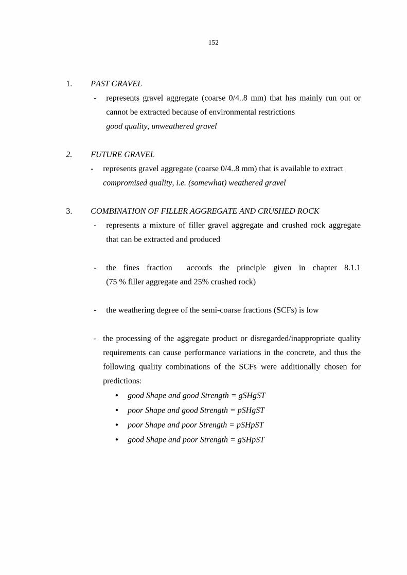
152
1. PAST GRAVEL
- represents gravel aggregate (coarse 0/4..8 mm) that has mainly run out or
cannot be extracted because of environmental restrictions
good quality, unweathered gravel
2. FUTURE GRAVEL
- represents gravel aggregate (coarse 0/4..8 mm) that is available to extract
compromised quality, i.e. (somewhat) weathered gravel
3. COMBINATION OF FILLER AGGREGATE AND CRUSHED ROCK
- represents a mixture of filler gravel aggregate and crushed rock aggregate
that can be extracted and produced
- the fines fraction accords the principle given in chapter 8.1.1
(75 % filler aggregate and 25% crushed rock)
- the weathering degree of the semi-coarse fractions (SCFs) is low
- the processing of the aggregate product or disregarded/inappropriate quality
requirements can cause performance variations in the concrete, and thus the
following quality combinations of the SCFs were additionally chosen for
predictions:
• good Shape and good Strength = gSHgST
• poor Shape and good Strength = pSHgST
• poor Shape and poor Strength = pSHpST
• good Shape and poor Strength = gSHpST

153
8.2 Predicting with the flow value model
8.2.1 SC- pore area 300-900 Å and SC- flakiness 3.15/4.0 mm vs. flow value
Figure 103 shows the combined effect of the SC- pore area 300-900Å and SC- flakiness
3.15/4.0 mm on the flow value for the six mix designs. The ranges of the SC- pore area
300-900 Å and the SC- flakiness are 0…0.13 m2/g and 1.23…1.43 respectively. The data
and corresponding coefficient of variation values are presented in appendix 6.
As can be seen from figure 103, there exists an apparent level difference between the low
and high paste mix designs. The effect of the increased amount of paste generally
exceeds the combined effect of SC- pore area and SC- flakiness, though there is some
overlapping. For all mix design groups the average flow value of the high paste mix
designs is greater than the maximum value for the low paste mix design (table 43).
Table 43. Statistics for the predicted flow value for each mix design; combined
effect of the SC- pore area 300-900Å and SC- flakiness 3.15/4.0 mm
N30 N35 AE30 AE35 WR30 WR35
Min [mm] 304 421 268 377 306 459
Max [mm] 470 570 427 503 535 700
Average [mm] 364 491 322 432 382 588
Stdev [mm] 50 43 45 39 64 67
The shape of the surfaces and the balance between the two characteristics on the surfaces
of the low paste mix designs are fairly identical. With a combination of low SC- pore
area and SC- flakiness, the flow value attains the highest values. The effect of the SC-
flakiness is, however, marginally greater than that of the SC- pore area.
With the high paste mix designs, the N35 and AE35 have similar types of surfaces, i.e.
when the SC- flakiness is low the effect of the SC- pore area is practically negligible. For

154
the WR35, however, the importance of the SC- pore area and SC- flakiness is
approximately equal to the flow value.
The superplasticizer enhances the quality differences between fine aggregate products
(table 43). In particular, the superplasticizer increases the workability of combinations
whose characteristics already produce best workability.
The coefficient of variation is highest in the area where both the SC- pore area and SC-
flakiness have high values, i.e. weathered and poor-shaped rock, which would normally
not be possible. Table 44 shows the coefficient of variation statistics for the predicted
flow value. More detailed information is given in appendix 6.
Table 44. Coefficient of variation statistics for the predicted flow value
for each mix design; combined effect of
the SC- pore area 300-900Å and SC- flakiness 3.15/4.0 mm
N30 N35 AE30 AE35 WR30 WR35
Min [%] 5 3 6 4 5 3
Max [%] 33 24 38 27 35 24
Average [%] 15 10 16 12 15 10
Stdev [%] 7 5 8 5 8 5

155
Figure 103. Combined effect of the SC- pore area 300-900Å and
SC- flakiness 3.15/4.0 mm on the flow value, all mix designs
0.000.010.030.040.060.070.090.100.120.13
1.23
1.28
1.32
1.36
1.41
300
350
400
450
500
550
600
Flo
w v
alu
e [m
m]
SC-pore area 300-900Å [m2/g]
SC-F
lkn
3/4
Flow N30
550-600
500-550
450-500
400-450
350-400
300-350
0.000.010.030.040.060.070.090.100.120.13
1.23
1.28
1.32
1.36
1.41
300
350
400
450
500
550
600
Flo
w v
alu
e [m
m]
SC-pore area 300-900Å [m2/g]
SC-F
lkn
3/4
Flow N35
550-600
500-550
450-500
400-450
350-400
300-350
0.000.010.030.040.060.070.090.100.120.13
1.23
1.28
1.32
1.36
1.41
250
300
350
400
450
500
550
Flo
w v
alu
e [m
m]
SC-pore area 300-900Å [m2/g]
SC-F
lkn
3/4
Flow AE30
500-550
450-500
400-450
350-400
300-350
250-300
0.000.010.030.040.060.070.090.100.120.13
1.23
1.28
1.32
1.36
1.41
250
300
350
400
450
500
550
Flo
w v
alu
e [m
m]
SC-pore area 300-900Å [m2/g]SC
-Flk
n 3/
4
Flow AE35
500-550
450-500
400-450
350-400
300-350
250-300
0.000.010.030.040.060.070.090.100.120.13
1.23
1.28
1.32
1.36
1.41
300
350
400
450
500
550
600
650
700
Flo
w v
alu
e [m
m]
SC-pore area 300-900Å [m2/g]
SC-F
lkn
3/4
Flow WR30
650-700
600-650
550-600
500-550
450-500
400-450
350-400
300-350
0.000.010.030.040.060.070.090.100.120.13
1.23
1.28
1.32
1.36
1.41
300
350
400
450
500
550
600
650
700
Flo
w v
alu
e [m
m]
SC-pore area 300-900Å [m2/g]
SC-F
lkn
3/4
Flow WR35
650-700
600-650
550-600
500-550
450-500
400-450
350-400
300-350

156
8.2.2 F- Cu and SC- flakiness 3.15/4.0 mm vs. flow value
Figure 104 shows the combined effect of the F- Cu and SC- flakiness 3.15/4.0 mm on the
flow value for the six mix designs. The ranges of F- Cu and SC- flakiness are 3.4…16.5
and 1.23…1.43 respectively. The data and corresponding coefficient of variation values
are presented in appendix 6.
The low and high paste surfaces are all fairly similar to each other, though the effect of
the SC- flakiness is slightly smaller in the case of mix designs with a high paste content.
Figure 104 and table 45 again show that in general, the amount of paste has a greater
effect on the flow value than the combined aggregate characteristics, though there is
some overlapping in the flow values of the same mix design group. The range of the flow
values is greater in the case of the low paste mix designs than in that of the high paste
mix designs, i.e. the additional paste and/or water reduces the combined effect of the F-
Cu and SC- flakiness.
Table 45. Statistics for the predicted flow value for each mix design;
combined effect of the F- Cu and SC- flakiness 3.15/4.0 mm
N30 N35 AE30 AE35 WR30 WR35
Min [mm] 332 465 302 414 331 586
Max [mm] 489 569 449 516 551 710
Average [mm] 394 513 353 457 428 663
Stdev [mm] 45 26 43 25 66 32
The flow value is highest when the F- Cu and SC- flakiness both have low values, and
correspondingly, it shows the lowest values when there is high F- Cu and SC- flakiness.
Again it can be noticed that the superplasticizer spreads the difference between the
extreme combinations.
The coefficient of variation statistics is presented in table 46. These values are
significantly smaller than the values for the SC- pore area and SC- flakiness

157
combination. As the fines and semi-coarse fractions were separated from each other, it
was possible to produce data over the whole combination range and thus, the quantiles
become smaller. More detailed information is given in appendix 6.
Table 46. Coefficient of variation statistics for the predicted flow value for each mix
design; combined effect of the F- Cu and SC- flakiness 3.15/4.0 mm
N30 N35 AE30 AE35 WR30 WR35
Min [%] 5 3 6 4 5 3
Max [%] 11 8 13 8 12 7
Average [%] 7 5 8 6 7 4
Stdev [%] 2 1 2 1 2 1

158
Figure 104. Combined effect of the Cu and flakiness 3.15/4.0 mm on the
flow value, all mix designs
356891112141516
1.23
1.28
1.32
1.36
1.41
300
350
400
450
500
550
600
Flo
w v
alu
e [m
m]
F - Cu SC-F
lkn
3/4
Flow N30
550-600
500-550
450-500
400-450
350-400
300-350
356891112141516
1.23
1.28
1.32
1.36
1.41
300
350
400
450
500
550
600
Flo
w v
alu
e [m
m]
F - Cu SC-F
lkn
3/4
Flow N35
550-600
500-550
450-500
400-450
350-400
300-350
356891112141516
1.23
1.28
1.32
1.36
1.41
250
300
350
400
450
500
550
Flo
w v
alu
e [m
m]
F - Cu SC-F
lkn
3/4
Flow AE30
500-550
450-500
400-450
350-400
300-350
250-300
356891112141516
1.23
1.28
1.32
1.36
1.41
250
300
350
400
450
500
550
Flo
w v
alu
e [m
m]
F - Cu SC-F
lkn
3/4
Flow AE35
500-550
450-500
400-450
350-400
300-350
250-300
356891112141516
1.23
1.28
1.32
1.36
1.41
300
350
400
450
500
550
600
650
700
750
Flo
w v
alu
e [m
m]
F - Cu SC-F
lkn
3/4
FlowWR30
700-750
650-700
600-650
550-600
500-550
450-500
400-450
350-400
300-350
356891112141516
1.23
1.28
1.32
1.36
1.41
300
350
400
450
500
550
600
650
700
750
Flo
w v
alu
e [m
m]
F - Cu SC-F
lkn
3/4
FlowWR35
700-750
650-700
600-650
550-600
500-550
450-500
400-450
350-400
300-350

159
8.2.3 Effect of different aggregate combinations on the flow value
Figure 105 presents predicted flow values including 10% and 90% quantiles for six
different aggregate combinations. The combinations are described in chapter 8.1.2.
Figure 105. Predicted flow values for six different aggregate combinations
The past gravel (PG) achieves the best flow values in the case of all mix designs. The
difference between the PG and future gravel (FG) constitutes approximately one
workability class, i.e. 60 mm, for the N and AE mix designs,while for the WR castings
the difference increases to two workability classes.
The flow values for the good-shaped crushed rock product (gSH) are at the same level as
in the case of the FG mix designs, with the exception of the WR35 mix design; in this
case the gSH attains the flow value of the PG. For the poor-shaped crushed rock (pSH)
the workability loss is severe for the mix designs containing the low amount of paste, but
when the paste amount is high mix designs the pSH mix designs achieve the flow values
of the FG.
Flow [mm] - predicted values incl. 10%-90% quantiles
gSH - pSTpSH - pSTpSH - gSTgSH - gSTFUTUREeeGRAVEL
WR30/35
AE30/35
N30/35
PAST…..hj GRAVEL
200
300
400
500
600
700
800

160
8.3 Predicting with the air % model
8.3.1 SC- Pore area 60-300 Å and SC- flakiness 3.15/4.0 mm vs. air %
Figure 106 shows the combined effect of the SC- pore area 60-300Å and SC- flakiness
3.15/4.0 mm on the air % for the AE mix designs. The ranges of the Sc- pore area and the
SC- flakiness are 0…0.14 m2/g and 1.23…1.43 respectively. The data and corresponding
coefficient of variation values are presented in appendix 6.
In both the AE mix designs the air % is mainly influenced by the SC- pore area. For the
higher SC- pore area values, the air % is well below the target value of 5%, and when the
SC- pore area value reduces approximately to the level of 0.05 m2/g the air % rises
rapidly. In the case of the low paste mix design the SC- flakiness tends to decrease the air
% while for the high paste mix design the Sc- flakiness increases the air %.
The quantiles for the expectation values are very high in the case of the higher SC- pore
area values. This is due to a lack of training data, i.e. no combination of high SC- pore
area and high SC- flakiness, and the different behaviour of aggregate products in the case
of the SC- pore area. Table 47 shows the statistics for the predicted air %. More detailed
information is given in appendix 6.
Table 47. Statistics for the predicted air %, AE mix designs
combined effect of the SC- pore area 60-300Å and SC- flakiness 3.15/4.0
mm
Predicted air % [%] Coefficient of variation [%]
AE30 AE35 AE30 AE35
Min 1.8 2.3 13 11
Max 5.1 6.6 111 112
Average 2.6 3.4 69 67
Stdev 1.0 1.2 33 32

161
Figure 106. Combined effect of the SC- pore area 60-300Å and
SC- flakiness 3.15/4.0 mm on the air %, AE mix designs
8.3.2 SC- pore area 60-300 Å and F- Cu vs. air %
Figure 107 shows the combined effect of the SC- pore area 60-300Å and F- Cu on the air
% for the AE mix designs. The ranges of the SC- pore area and F- Cu are 0…0.14 m2/g
and 3.4…16.5 respectively. The data and corresponding coefficient of variation values
are presented in appendix 6.
The combined effect of the SC- pore area and F- Cu is very similar to the effect of the
SC- pore area and SC- flakiness. The air % is low for high SC- pore area values and rises
when the pore area of the semi-coarse fraction decreases. When the semi-coarse fraction
has low pore area values, the influence of the F- Cu can be detected. The air % becomes
higher if the Cu value of the fines is low.
The quantiles for the expectation values are very high with the higher SC- pore area
values. This is due to the different behaviour of aggregate products in the case of the SC-
pore area. Table 48 shows the statistics for the predicted air %. More detailed
information is given in the appendix 6.
0.00 0.02 0.03 0.05 0.06 0.08 0.10 0.11 0.13 0.141.23
1.28
1.32
1.36
1.41
1
2
3
4
5
6
7
Flo
w v
alu
e [m
m]
SC-pore area 60-300Å [m2/g]
SC-F
lkn
3/4
Air %AE30
6-7
5-6
4-5
3-4
2-3
1-2
0.00 0.02 0.03 0.05 0.06 0.08 0.10 0.11 0.13 0.141.23
1.28
1.32
1.36
1.41
1
2
3
4
5
6
7
Flo
w v
alu
e [m
m]
SC-pore area 60-300Å [m2/g]
SC-F
lkn
3/4
Air %AE35
6-7
5-6
4-5
3-4
2-3
1-2

162
Table 48. Statistics for the predicted air %, AE mix designs
combined effect of the SC- pore area 60-300Å and F- Cu
Predicted air % [%] Coefficient of variation [%]
AE30 AE35 AE30 AE35
Min 1.7 2.3 15 12
Max 4.7 5.9 108 100
Average 2.6 3.4 68 64
Stdev 0.9 1.2 34 33
Figure 107. Combined effect of the SC- pore area 60-300Å and F- Cu on the air %,
AE mix designs
0.00 0.02 0.03 0.05 0.06 0.08 0.10 0.11 0.13 0.143
6
9
12
15
1
2
3
4
5
6
7
Flo
w v
alu
e [m
m]
SC-pore area 60-300Å [m2/g]
F - C
u
Air %AE30
6-7
5-6
4-5
3-4
2-3
1-2
0.00 0.02 0.03 0.05 0.06 0.08 0.10 0.11 0.13 0.143
6
9
12
15
1
2
3
4
5
6
7
Flo
w v
alu
e [m
m]
SC-pore area 60-300Å [m2/g]
F - C
u
Air %AE35
6-7
5-6
4-5
3-4
2-3
1-2

163
8.3.3 Effect of different aggregate combinations on the air %
Figure 108 presents predicted air % values including 10% and 90% quantiles for six
different aggregate combinations. The combinations are described in chapter 8.1.2.
Figure 108. Predicted air % for six different aggregate combinations
For the N and WR mix designs the air % describes the amount of unintentionally
entrapped air i.e. air that is in the concrete due to unsuccessful compaction and low
workability. Generally can be noticed that the entrapped air is higher for the mix designs
containing the low amount of paste and for the poor-shaped aggregate products. The mix
designs containing the high amount of paste and the crushed products have entrained air
% values equal to those mix designs made with the past and future gravel products. By
contrast, the low paste AE30 containing crushed aggregate product attains significantly
lower air % values than those of the corresponding high paste mix design. The difference
is even greater if the shape is bad.
AIR% -predicted values incl. 10%-90% quantiles
gSH - pST..pSH - pST..pSH - gST..gSH - gST..
N30/35
AE30/35
WR30/35
PAST…..…. GRAVEL
FUTURE.....GRAVEL
0
1
2
3
4
5
6
7

164
8.4 Predicting with the bleeding model
8.4.1 SC- total pore area and F- BET value vs. bleeding
Figure 109 shows the combined effect of the SC- total pore area and F- BET on the
bleeding for the N35 and WR35 mix designs. The ranges of the SC- total pore area and
F- BET are 0.01…0.34 m2/g and 1.3…14.0 m2/g respectively. The data and
corresponding coefficient of variation values are presented in appendix 6.
For the N35 mix design the effect of the fines, i.e. the F- BET value, is stronger than the
effect of the semi-coarse, i.e. the SC- total pore area. The bleeding is highest when the F-
BET value and SC- total pore area both have low values, i.e. the combined pore area of
the fines and semi-coarse factions is the smallest.
For the WR35 mix design the effect of the F- BET and SC- total pore area is roughly
equal. The bleeding phenomenon of the mix designs N35 and WR35 differ from each
other. When the bleeding of the N35 mix design increases linearly as the combined pore
area decreases, the bleeding of the mix design WR35 is low, until a threshold value for
the combined pore area has been reached, after which the bleeding increases drastically.
The quantiles of the expectation values are very high over the whole 3D surface area.
Reasons for this include the different behaviour of aggregate products regarding the pore
area characteristics, inaccuracies in the measurements and small absolute values. It has
also already been noted that the model underestimates the high bleeding values, and thus
the quantiles become additionally larger in this area. Table 49 shows the statistics for the
predicted bleeding. More detailed information is given in appendix 6.

165
Table 49. Statistics for the bleeding, N35 and WR35 mix designs
combined effect of SC- total pore area and F- BET value
Predicted bleeding [g/cm3] Coefficient of variation [%]
N35 WR35 N35 WR35
Min 3.3 0.2 28 47
Max 7.5 13.3 194 147
Average 4.5 1.8 86 87
Stdev 1.1 2.3 43 27
Figure 109. Combined effect of the SC- total pore area and F- BET on the bleeding;
N35 and WR35 mix designs
8.4.2 SC- total pore area and SC- elongation 0.8/1.0 mm vs. bleeding
Figure 110 shows the combined effect of the SC- total pore area and SC- elongation
0.8/1.0 mm on the bleeding for the N35 and WR35 mix designs. The ranges of the SC-
total pore area and SC- elongation 0.8/1.0 mm are 0.01…0.34 m2/g and 1.45…1.64
respectively. The data and corresponding coefficient of variation values are presented in
appendix 6.
0.010.05
0.080.120.160.190.230.260.300.34
14
7
10
13
0
2
4
6
8
10
12
14
Ble
edin
g [g
/cm
3 ]
SC-tot. pore area [m2/g]
BET [m2/g
]
BleedingWR35
12-14
10-12
8-10
6-8
4-6
2-4
0-2
0.010.05
0.080.120.160.190.230.260.300.34
1
4
7
10
13
0
1
2
3
4
5
6
7
Ble
edin
g [g
/cm
3 ]
SC-tot. pore area [m2/g]BET [m
2/g]
BleedingN35
6-7
5-6
4-5
3-4
2-3
1-2
0-1

166
For the N35 mix design the effect of the SC- total pore area and SC- elongation is
roughly equal. The highest bleeding values occur when the SC- total pore area is low and
the SC- elongation has average range values.
For the WR35 mix design the SC- total pore area has a much greater impact than the SC-
elongation. In the high SC- total pore area the bleeding values are very minimal, and
after a threshold value for the SC- total pore area has been reached, the bleeding
increases rapidly. The highest bleeding value occurs when the SC- total pore area is low
and the SC- elongation is high.
The quantiles of the expectation values are very high over the whole 3D surface area.
Reasons for this include the different behaviour of aggregate products regarding the pore
area characteristics, inaccuracies in the measurements and small absolute values. It has
also already been noted that the model underestimates the high bleeding values, and thus
the quantiles become additionally larger in this area. Table 50 shows the statistics for the
predicted bleeding. More detailed information is given in appendix 6.
Table 50. Statistics for the bleeding, N35 and WR35 mix designs
combined effect of SC- total pore area and SC- elongation 0.8/1.0 mm
Predicted bleeding [g/cm3] Coefficient of variation [%]
N35 WR35 N35 WR35
Min 2.3 0.9 26 27
Max 6.8 11.2 220 148
Average 4.9 3.2 70 77
Stdev 1.2 2.6 39 28

167
Figure 110. Combined effect of the SC- total pore area and SC- elongation 0.8/1.0 mm
on the bleeding; N35 and WR35 mix designs
8.4.3 Effect of different aggregate combinations on the bleeding
Figure 111 presents predicted bleeding values includeing 10% and 90% quantiles for six
different aggregate combinations. The combinations are described in chapter 8.1.2.
Figure 111. Predicted bleeding for six different aggregate combinations
0.01 0.05 0.08 0.12 0.16 0.19 0.23 0.260.30
0.34
1.45
1.50
1.54
1.58
1.62
0
1
2
3
4
5
6
7
Ble
edin
g [g
/cm
3 ]
SC-tot. pore area [m2/g] SC-Elg
n 0.8/1
Bleeding N35
6-7
5-6
4-5
3-4
2-3
1-2
0-1
0.01 0.05 0.08 0.12 0.16 0.19 0.23 0.260.30
0.34
1.45
1.50
1.54
1.58
1.62
0
1
2
3
4
5
6
7
Ble
edin
g [g
/cm
3 ]
SC-tot. pore area [m2/g] SC-Elgn 0.8/1
BleedingWR35
6-7
5-6
4-5
3-4
2-3
1-2
0-1
Bleeding [g/cm3]- predicted values incl. 10%-90% quantiles
gSH -. pSTpSH -. pSTpSH - .gSTgSH -. gSTFUTURE..eGRAVEL
WR30/35
AE30/35
N30/35
PAST…... . GRAVEL
0
2
4
6
8
10
12
14

168
The past gravel has higher bleeding values than the future gravel for all mix designs. The
crushed aggregate combinations exhibit bleeding phenomena similar to those of the past
gravel, except the good-shapes WR35, which has significantly higher bleeding. The
quantiles are also very large for the good-shaped WR35 mix design.
8.5 Predicting with the compressive strength model
8.5.1 SC- Los Angeles value and SC- flakiness 3.15/4.0 mm vs. compressive strength
Figure 112 shows the combined effect of the SC- Los Angeles value and SC- flakiness
3.15/4.0 mm on the compressive strength for the six mix designs. The ranges of the SC-
Los Angeles value and SC- flakiness are 19.6…38.2 % and 1.23…1.43 respectively. The
data and corresponding coefficient of variation values are presented in appendix 6.
The surfaces of the N and WR mix designs are controlled by changes in the SC- Los
Angeles value, and the influence of the SC- flakiness only marginally modifies the shape
of the 3D surface. The effects of the SC- flakiness are mainly due to the influence on the
workability, i.e. compaction degree of concrete, and strength properties of individual
aggregate particles. Both the N30 and WR30 have the lowest compressive strength
values with a combination of high SC- Los Angeles value and high SC- flakiness. In the
case of mix designs with the high paste amount the phenomenon is weaker. The WR mix
designs have the highest compressive strength values when both the SC- Los Angels and
SC- flakiness have low values. In contrast, the high paste N35 has the highest
compressive strength with a combination of low SC- Los Angels value and high SC-
flakiness. For the low paste N30 the effect of the SC- flakiness in the low SC- Los
Angeles value area is almost negligible. The gain of the compressive strength for the AE
mix designs is strongly dependent on the entrained air. Even so, high SC- Los Angeles
values do also affect the compressive strength of the AE mix designs negatively.

169
The range of the compressive strength values is the greatest for the WR mix designs and
the low paste N30 (table 51).
Table 51. Statistics for the predicted compressive strength for each mix design;
combined effect of the SC- Los Angeles value and SC- flakiness 3.15/4.0
mm
N30 N35 AE30 AE35 WR30 WR35
Min [MPa] 42 45 45 41 50 52
Max [MPa] 51 51 50 47 62 62
Average [MPa] 46 47 47 44 58 57
Stdev [MPa] 2.1 1.3 1.2 1.4 2.6 2.1
The quantiles of the expectation values are highest in the corners of the high SC- Los
Angeles value and low SC- flakiness as well as in those of low SC- Los Angeles value
and high SC- flakiness. Table 52 shows the coefficient of variation statistics for the
predicted compressive strength. More detailed information is given in appendix 6.
Table 52. Coefficient of variation statistics for the predicted compressive strength
value for each mix design;
combined effect of the SC- Los Angeles value and SC- flakiness 3.15/4.0
mm
N30 N35 AE30 AE35 WR30 WR35
Min [%] 2 2 2 2 2 2
Max [%] 8 8 8 9 8 9
Average [%] 3 3 4 4 3 3
Stdev [%] 1 1 1 1 1 2

170
Figure 112. Combined effect of the SC- Los Angeles value and
SC- flakiness 3.15/4.0 mm on the compressive strength; all mix designs
202224262830323436
38
1.231.28
1.32
1.36
1.41
42
44
46
48
50
52
Co
mp
. Str
eng
th [
MP
a]SC-LA value (mod.) [%]
SC-Flkn 3/4
C 91dN30
50-52
48-50
46-48
44-46
42-44
202224262830323436
38
1.231.28
1.32
1.36
1.41
42
44
46
48
50
52
Co
mp
. Str
eng
th [
MP
a]
SC-LA value (mod.) [%]
SC-Flkn 3/4
C 91dN35
50-52
48-50
46-48
44-46
42-44
20222426283032343638
1.23
1.28
1.32
1.36
1.41
40
42
44
46
48
50
52
Co
mp
. Str
eng
th [
MP
a]
SC-LA value (mod.) [%]
SC-Flkn 3/4
C 91dAE30
50-52
48-50
46-48
44-46
42-44
40-42
202224262830323436
38
1.231.28
1.32
1.36
1.41
40
42
44
46
48
50
52
Co
mp
. Str
eng
th [
MP
a]
SC-LA value (mod.) [%]
SC-Flkn 3/4
C 91dAE35
50-52
48-50
46-48
44-46
42-44
40-42
202224262830323436
38
1.23
1.28
1.32
1.36
1.41
50
52
54
56
58
60
62
64
Co
mp
. Str
eng
th [
MP
a]
SC-LA value (mod.) [%]
SC-Flkn 3/4
C 91dWR30
62-64
60-62
58-60
56-58
54-56
52-54
50-52
202224262830323436
38
1.23
1.28
1.32
1.36
1.41
50
52
54
56
58
60
62
64
Co
mp
. Str
eng
th [
MP
a]
SC-LA value (mod.) [%]
SC-Flkn 3/4
C 91dWR35
62-64
60-62
58-60
56-58
54-56
52-54
50-52

171
8.5.2 SC- Los Angeles value and SC- pore area 60-300 Å vs. compressive strength
Figure 113 shows the combined effect of the SC- Los Angeles value and SC- flakiness
3.15/4.0 mm on the compressive strength for the six mix designs. The ranges of the SC-
pore area 60-300 Å and SC- Los Angeles value are 0…0.14 m2/g and 19.6…38.2%
respectively. The data and corresponding coefficient of variation values are presented in
appendix 6.
The N and AE mix designs have similar 3D surface shapes, whereas the WR mix designs
deviate fundamentally from their shape. The effect of the SC- pore area on the
compressive strength of the WR mix designs is minimal, and thus the combined effect of
the SC- pore area and SC- Los Angeles value is mainly dominated by the SC- Los
Angeles value changes. The highest and lowest predicted compressive strength values for
the WR mix designs are in the corners of low SC- pore area and low SC- Los Angeles
value and of high SC- pore area and high SC- Los Angeles value. For the N mix designs
the surface cambers approximately in the middle of the SC- pore area range, where the
compressive strength also reaches the highest value for each SC- Los Angeles value. The
AE mix designs camber similarly and also on the zero SC- pore area line, where the
compressive strength values are balanced between the strength of the aggregate (Los
Angeles value) and entrained air %.
The statistics for the predicted compressive strength values are presented in table 53. The
range of the compressive strength values is the greatest for the WR mix designs and the
low paste N30. The quantiles of the expectation values are highest in the high SC- pore
area. Table 54 shows the coefficient of variation statistics for the predicted compressive
strength. More detailed information is given in appendix 6.

172
Table 53. Statistics for the predicted compressive strength for each mix design;
combined effect of the SC- Los Angeles value and SC-pore area 60-300 Å
N30 N35 AE30 AE35 WR30 WR35
Min [MPa] 45 46 47 43 51 51
Max [MPa] 52 52 53 50 61 60
Average [MPa] 47 48 50 47 57 56
Stdev [MPa] 2.0 1.5 1.4 1.6 2.9 2.6
Table 54. Coefficient of variation statistics for the predicted compressive
strength value for each mix design;
combined effect of the SC- Los Angeles value and SC-pore area 60-300 Å
N30 N35 AE30 AE35 WR30 WR35
Min [%] 2 2 2 2 6 26
Max [%] 11 10 10 10 11 11
Average [%] 6 5 5 5 5 5
Stdev [%] 2 2 2 2 2 2

173
Figure 113. Combined effect of the SC- Los Angeles value and
SC- pore area 60-300 Å on the compressive strength; all mix designs
0.000.020.030.050.060.080.100.110.130.14
2024
28
32
36
44
46
48
50
52
54
Co
mp
. Str
eng
th [
MP
a]
SC-pore area 60-300Å [m2/g] SC-LA value (mod)
C 91dN30
52-54
50-52
48-50
46-48
44-46
0.000.020.030.050.060.080.100.110.130.14
2024
28
32
36
44
46
48
50
52
54
Co
mp
. Str
eng
th [
MP
a]
SC-pore area 60-300Å [m2/g] SC-LA value (mod)
C 91dN35
52-54
50-52
48-50
46-48
44-46
0.000.020.030.050.060.080.100.110.130.14
20
24
28
32
36
42
44
46
48
50
52
54
Co
mp
. Str
eng
th [
MP
a]
SC-pore area 60-300Å [m2/g]
SC-LA value (mod)
C 91dAE30
52-54
50-52
48-50
46-48
44-46
42-44
0.000.020.030.050.060.080.100.110.130.14
20
24
28
32
36
42
44
46
48
50
52
54
Co
mp
. Str
eng
th [
MP
a]
SC-pore area 60-300Å [m2/g]
SC-LA value (mod)
C 91dAE35
52-54
50-52
48-50
46-48
44-46
42-44
0.000.020.030.050.060.080.100.110.130.14
2024
28
32
36
50
52
54
56
58
60
62
Co
mp
. Str
eng
th [
MP
a]
SC-pore area 60-300Å [m2/g] SC-LA value (mod)
C 91dWR30
60-62
58-60
56-58
54-56
52-54
50-52
0.000.020.030.050.060.080.100.110.130.14
2024
28
32
36
50
52
54
56
58
60
62
Co
mp
. Str
eng
th [
MP
a]
SC-pore area 60-300Å [m2/g] SC-LA value (mod)
C 91dWR35
60-62
58-60
56-58
54-56
52-54
50-52

174
8.5.3 Effect of different aggregate combinations on the compressive strength
Figure 114 presents predicted compressive strength values including 10% and 90%
quantiles for six different aggregate combinations. The combinations are described in
chapter 8.1.2.
Figure 114. Predicted compressive strength values for six different aggregate
combinations
There is no significant compressive strength difference between the past gravel, future
gravel and crushed rock product with good shape and good strength. If it has a good
strength, even concrete made of crushed rock product with a poor shape achieves a
quality similar to that of the N and AE mix designs, though some loss of compressive
strength occurs with the WR mix designs. A remarkable loss of compressive strength
ensues if the fine aggregate combination has both poor shape and poor strength. The
difference to PG is between 5 – 10 MPa for the N and AE mix designs and between 10-
15 MPa for the WR mix designs. If a product exhibiting poor strength is made with good
shape, the loss is prevented in the case of the N35 and AE mix designs. In the case of the
low paste N30 mix design some loss can be expected, and in the case of the WR mix
designs the loss is between 5-10 MPa.
Comp. strength [MPa] - predicted values incl. 10%-90% quantiles
gSH - pST.pSH - pST.pSH - gST.gSH - gST.
WR30/35
AE30/35
N30/35
FUTURE…GRAVEL
PAST…..…GRAVEL
35
40
45
50
55
60
65

175
8.6 Discussion of the predictions made with the models
The models were based on the outlines made with the fine aggregate and mix design
selections. The following considerations can be applied to the models:
• The selected fine aggregate products represent fairly well the common Finnish
variety range of concrete aggregates used in Finland, as well as representing products
that might replace the familiar fine aggregate solutions in the future, i.e. weathered
gravel and crushed rock products.
• All castings had the same grading curve (close to the ideal grading curve).
• The coarse aggregate was uncrushed gravel and was the same in all castings
• Castings were divided into six mix designs: cement amount 300 kg/m3 or 350 kg/m3,
no admixture w/c=0.65, superplasticizer w/c=0.58, air-entraining agent w/c=0.58
• The average compressive strength was 45 MPa – 55 MPa (no additives were used).
• The models were made for concrete with a maximum aggregate size of 14 mm
Table 56 presents a summary of the concrete properties made with the six aggregate
combinations (see chapter 8.1.2 and appendix 5). The points given to each aggregate-mix
design composition represent how much the concrete property value of the evaluated
aggregate combination deviated from the value attained with the past gravel. The rules
for the point scoring are shown in table 55. The deviations were calculated from the
expectation values.
Table 55. Rules for the point scoring for concrete property deviation between
the past gravel and the fine aggregate combination evaluated
Points per
deviation
Flow value
[mm]
Air %
[%]
Bleeding
[g/cm3]
Compressive strength
[MPa]
1 ± 50 ± 0.5 ± 2 ± 5
2 ± 100 ± 1.0 ± 4 ± 10
3 ± 150 ± 1.5 ± 6 ± 15
4 ± 200 ± 2.0 ± 8 ± 20

176
Table 56. Summary of the modelled concrete property values as
compared against the values for the past gravel
Fine aggregate combination
Future gravel
Good shape-
good strength
Poor shape-
good strength
Poor shape-
poor strength
Good shape-
poor strength
-1 -1 -3 -3 -1-1 0 -1 -1 0-1 -1 -2 -2 -1-1 0 -1 -1 0-2 -2 -4 -4 -2-2 0 -2 -2 0FL
OW
VA
LU
E
N30
N35
AE30
AE35
WR30
WR35
TOTAL -8 -4 -13 -13 -4-1 0 0 0 0-1 0 -1 -1 00 0 -2 -2 00 0 0 0 0-1 0 -2 -2 0-1 0 -1 -1 0
AIR
%
N30
N35
AE30
AE35
WR30
WR35
TOTAL -4 ±±±±0 -6 -6 ±±±±0+1 0 0 0 0+1 0 0 0 00 0 0 0 00 0 0 0 00 0 0 0 0
+1 -2 0 0 -2BL
EE
DIN
G
N30
N35
AE30
AE35
WR30
WR35
TOTAL +3 -2 ±±±±0 ±±±±0 -20 0 0 -2 00 0 0 -1 00 0 0 -1 00 0 0 -2 00 0 -1 -3 -20 0 0 -2 -1
CO
MPR
ESS
IVE
STR
EN
GT
H
N30
N35
AE30
AE35
WR30
WR35
TOTAL ±±±±0 ±±±±0 -1 -11 -3

177
If all six mix designs are included, the past gravel has by far the best workability, i.e.
flow value. The good-shaped rock, however, has equal workability if the amount of paste
is sufficient. On lower amounts of paste, the good-shaped rock has flow values equal to
those for the future gravel, which represents uncrushed gravel with weathering
properties. The loss in workability is considerable if the rock product is of poor shape,
and the influence, is strongest with the low paste mix designs.
The compressive strength values were same with the past gravel, future gravel and with
good-shape & good-strength rock. Even if the rock has poor shape, but if its strength is
good, the compressive strength values of the concrete are nearly equal to those of the past
gravel. Only some strength loss is expected with the WR30 mix design. If the aggregate,
on the other hand, has poor strength but a good shape, then the compressive strength loss
starts to build up, especially with the superplasticizer mix designs. If, however, both the
shape and strength are poor, then the compressive strength of the concrete is significantly
lower than that of the past gravel.
The future gravel and the good-shaped & good-strength rock both need extra water to
attain the same workability as the past gravel. Because there was no difference in the
compressive strength over the past gravel, any extra water added to increase the flow
value of the future gravel and of the good-shaped & good-strength rock leads to lower
compressive strength. We can thus conclude that even if the effective mix design
procedure would (most likely) raise the flow value of the future gravel to the same level
as the past gravel, it would in any case cause a reduction in the compressive strength.
Additionally, increasing the workability with cement paste will have economic
consequences, though to a much lesser degree than with the poor-shaped and good-
shaped & poor strength rock products. It is even uncertain if the same compressive
strength level as that of the past gravel can be reached, since both the workability and the
compressive strength are so greatly compromised.
The deviations in the air % are caused mainly by the low workability, and the
unsuccessful compaction and, for the AE mix designs, the unsuccessful air formation. It

178
is not possible to evaluate the quality of the entrained air on the basis of the amount of air
in the AE mix designs.
The future gravel, in general, reduces the bleeding tendency as a result of the particle
porosity characteristics. The good-shaped rock products, however, have a greatly
increased tendency for bleeding and even for segregation with the high paste concrete
with superplasticizer. This is also due to the particle porosity phenomenon, but in this
case the explanation is, more specifically, the lack of particle porosity.
Some of the concrete properties could be controlled by other mix design changes, e.g. by
adding additives and by changing the grading curve. One example is the workability of
the good-shaped rock product which, most likely, with a finer grading curve and/or
added additive could be adjusted without extra water to have a flow value equal to that of
the past gravel. The finest particles could reduce the friction between the semi-coarse
particles and to increase the packing density by filling the interstitial spaces between
them. This does not apply to the future gravel, as it has round/non-angular particles, but
anyhow worse workability than the past gravel.
The superplasticizer enhances the difference between the fine aggregate products, e.g. the
relative difference between the flow values of two fine aggregate combinations is greater
with the mix design containing the superplasticizer than without the admixture. This is
also the case with the compressive strength, though the strength level is higher with the
WR than with the N and AE mix designs; this, in turn, can influence the impact of the
inputs, e.g. the Los Angeles value. The superplasticizer also seems to affect how the
particle porosity characteristics affect the compressive strength. For the N and AE mix
designs there appears to be an optimum particle porosity level for the semi-coarse
fraction, whereas, no such point exists for the WR mix designs.

179
9. VERIFICATION OF THE MODELS WITH
TWO NEW AGGREGATE PRODUCTS
9.1 Procedure
The verification of the models was performed by introducing two such aggregate
products that had not been utilized in the modelling of the interaction between aggregate
characteristics and concrete properties. The aggregate products consisted of the fines and
semi-coarse fractions.
First the aggregate products were investigated with the same methods that are described
in the chapter 4.4 to obtain the input values for the models. Secondly, castings with the
mix designs N35, WR30 and AE35 were executed with both of the aggregate products.
Finally, the actual results were compared against the values attained from the models. In
the comparison is taken into account the repeatability error of the councrete
measurements (actual results) as well as the 10 % and 90 % quantiles for the modelled
values.
9.2 Identification of the new aggregate products
The aggregate input values of the two new aggregates are shown in table 57. The table
includes the aggregate characteristics for both the fines (F) and the semi-coarse (SC)
fractions. Additionally, the table presents which aggregate inputs are valid for each
model, e.g. flow value, air %, bleeding and compressive strength 91 d.
The A1 is a crushed rock and by rock type it is categorized as granite. The B16 is an
uncrushed granitic gravel.

180
Table 57. Aggregate input values of the B16 and A1 aggregate products
9.3 Results of the modelled and measured values
The results of the models include the expectation values and their 10% and 90 %
quantiles, whereas the measured values are presented by the actual values and their
repeatability ranges (chapter 6).
In each of the following figures the symbols are the same:
Asterisk ( * ) actual value
Box ( ) repeatability range of the actual value
Diamond ( ♦ ) expectation value (modelled value)
Line ( ) 10 –90 % quantiles of the expectation value
B16/B16 A1/A1 FLOW AIR % BLEEDING
COMP. STRENGTH 91d
BET 2,27 1,31 X X XF - density [Mg/m3] 2,7726 2,6711 XF - Zeta pot. [mV] -9,1 -11,2 X XF - Cu 6 14,6 X X XSC-avg. pore size [um] 1,74 9,72 XSC-tot. pore area [m2/g] 0,05 0,013 XSC-LA value (mod.) [%] 21,8 36,9 XSC-Elgn 3.15/4.0 mm 1,37 1,44 XSC-Elgn 1.6/2.0 mm 1,38 1,49 XSC-Elgn 0.8/1.0 mm 1,45 1,6 XSC-Angularity 4,9 7,14 X XSC-Qnty 1.6/2.0 mm 16610000 17000000 XSC-Flkn 3.15/4.0 mm 1,25 1,36 X X XSC-Flkn 1.6/2.0 mm 1,25 1,37 XF-mica [%] 1 3 XSC-pore area>900Å [m2/g] 0,022 0,009 XSC-pore area 300-900Å [m2/g] 0,005 0 X XSC-pore area 60-300Å [m2/g] 0,001 0 X X

181
Figure 115. Verification of the flow value model
Figure 116. Verification of the air % model
A1/A1 AE35
B16/B16 N35
B16/B16 WR30
B16/B16 AE35
A1/A1 WR30
A1/A1 N35
330 380 430 480 530 580 630
A1/A1 AE35
B16/B16 N35
B16/B16 WR30
B16/B16 AE35
A1/A1 WR30
A1/A1 N35
0 1 2 3 4 5 6 7 8
Air [ % ]
Flow value [mm]

182
Figure 117. Verification of the bleeding model
Figure 118. Verification of the compressive strength model
A1/A1 AE35
B16/B16 N35
B16/B16 WR30
B16/B16 AE35
A1/A1 WR30
A1/A1 N35
38 43 48 53 58 63 68
A1/A1 AE35
B16/B16 N35
B16/B16 WR30
B16/B16 AE35
A1/A1 WR30
A1/A1 N35
0 1 2 3 4 5 6 7 8
Compressive strength 91d [ MPa]
Bleeding [ g/cm3]

183
9.4 Evaluation of the verification of the modelled and measured values
The evaluation of the models is carried out by comparing the modelled and measured
values and by detecting if the ranges of the 10 – 90 % quantiles and repeatability are
overlapping. If the modelled value is inside the repeatability range, it can be stated that
the modelled value is within the 95 % confidence interval of the measurement. If instead
only the repetabilty range and the quantiles of the 10 – 90 % overlap, then can be stated
that due to the model error there exists a statistical probability that the modelled and
measured values are equal. However, that cannot be statistically proved.
Table 58. Evaluation of the accuracy of the modelled and measured values for
the verification castings (N35, WR30 and AE35)
Modelled value inside the
measurement repeatability
Measurement repeatability
and quantiles of the model
overlap
B16 A1 B16 A1
Flow value 2 of 3 1 of 3 1 of 3 2 of 3
Air % 1 of 3 2 of 3 2 of 3 1 of 3
Bleeding 2 of 3 2 of 3 1 of 3 1 of 3
Compressive strength 91 d 2 of 3 1 of 3 1 of 3 2 of 3
As a conclusion one can say that the model predicted the actual behaviour of uncrushed
gravel B16 very well and the crushed rock A1 satisfactorily.

184
10. CONCLUSIONS
The results for aggregate and concrete as well as the results for the models are based on
21 aggregate products and 215 castings made with six different mix designs. The mix
designs consisted of two cement amounts (300 or 350 kg/m3) corresponding to low and
high paste volumes, with three admixture possibilities: no admixture, superplasticizer or
air-entraining agent.
The following listing of the conclusions is divided into seven headlines. The four first
ones are the modelled concrete parameters; flow value, compressive strength, air % and
bleeding. The three next groups are the drying shrinkage, the aggregate characteristics
and the aggregate testing methods.
FLOW VALUE
1. For the same mix design, the flow value differed according to the quality
characteristics of the fine aggregate, and ranged between 150...295 mm, i.e.
2.5…5 workability classes. The greater variations were observed with the low
paste mix designs. (concrete test results)
2. The most important fine aggregate characteristics in the flow value model were
the semi-coarse fraction parameters related to shape and particle porosity. Even
though the amount of paste was the decisive parameter in determining the general
level of the flow value, the effect of the fine aggregate characteristics could
exceed the effect of the paste difference. For the no-admixture and air-entraining
agent mix designs, the average effect of the paste difference was 100 mm, and for
the superplasticizer mix designs it was 200 mm. The flow model error was 34
(32-38) mm and the repeatability error of the measurement represents 44% of the
model error. (model)
3. The weathering of gravel affected the flow value more negatively than the use of
a combination of good-shaped rock as the semi-coarse fraction and unweathered
filler aggregate as the fines. If the shape of the rock semi-coarse fraction was
poor, the reduction observed in the flow value was extensive, especially if the
paste amount was low. For the low paste mix designs the reduction was up to
185
100…200 mm, i.e. 1.5…3.5 workability classes, dependent of the mix design and
for the high paste amount the reduction was up to 50…100 mm.
(model/sensitivity analysis, predictions with the model)
4. The superplasticizer enhanced the difference in quality between fine aggregate
products. The relative difference between the flow values of two fine aggregate
products was greater with superplasticizer mix designs than with mix designs
without any admixture or with the air-entraining agent. (concrete test results &
predictions with the model)
COMPRESSIVE STRENGTH
5. For the same mix design, the compressive strength differed according to the
quality characteristics of the fine aggregate, and ranged between 8.4…18.8 MPa.
The largest variation was detected with the superplasticizer mix designs. The
average compressive strength of the mix designs varied between approximately
45 – 55 MPa. (concrete test results)
6. The most important fine aggregate characteristics for the compressive strength
model were the flakiness 3.15/4.0 mm and the Los Angeles value of the semi-
coarse fraction. The compressive strength model error was 2.7 (2.4-3.0) MPa, and
the repeatability error of the measurement represents 78% of the model error.
(model)
7. If the rock product was good-shaped and had good strength, then the compressive
strength of the concrete equalled that of the unweathered gravel. Even if the rock
had poor shape, if it had good strength the compressive strength was only
marginally affected. With the combination of poor strength and good shape, the
compressive strength with the superplasticizer mix designs was reduced by 5-10
MPa as compared to the unweathered gravel. (predictions with the model)
8. If the rock product had the combined characteristics of poor shape, i.e. flaky/thin
particles, and poor strength, the quality characteristics had a manifold negative
effect on the compressive strength. The compressive strength was reduced by as
much as 10-15 MPa with the superplasticizer mix designs and by 5-10 MPa with
mix designs having no admixture or having air-entraining agent (predictions with
the model)

186
9. The superplasticizer affected the bond between the aggregate particles and the
paste (see #8). The effect of the changes on the Los Angeles value was the
strongest with the superplasticizer mix designs as compared to mix designs
without any admixture or with the air-entraining agent. (model/sensitivity
analysis, predictions with the model)
10. For the no admixture and air-entraining agent mix designs, there was an optimum
particle porosity level for the semi-coarse fraction when the compressive strength
was the highest, but for the superplasticizer mix designs the effect of the particle
porosity of the semi-coarse fraction was linear. (predictions with the model)
AIR %
11. For same mix design, the air % differed according to the quality characteristics of
the fine aggregate and ranged between 1.1…1.8% for the no admixture and
superplasticizer mix designs and 4.5% for the air-entraining agent mix designs.
(concrete test results)
12. The amount of the entrapped and entrained air correlated strongly with the flow
value. Thus, the most important fine aggregate characteristics were the particle
porosity and shape related semi-coarse fraction parameters. The air % model
error was 0.6% (0.5-0.7%) and the repeatability error of the measurement
represents 50% of the model error. (model)
BLEEDING
13. For same mix design, the bleeding varied due to the quality characteristics of the
fine aggregate and ranged between 2.2…8.7 g/cm3 for all other mix designs
except for the high paste superplasticizer mix design, which had variation of 18.2
g/cm3. (concrete test results)
14. The most important parameters for the bleeding model were the superplasticizer
and the amount of paste. From the fine aggregate characteristics, the particle
porosity parameters of the semi-coarse fraction and surface area parameter for the
fines were important. Additionally, the shape parameters of the semi-coarse
fraction were important for the model, as they decreased the workability and thus
reduced the bleeding tendency. The bleeding model error was 1.8 (1.3-2.2) g/cm3

187
and the repeatability error of the measurement represents 72% of the model error.
(model)
15. The fine aggregate combination of good-shaped rock as the semi-coarse fraction
and unweathered filler aggregate as fines, greatly increased the tendency for
bleeding and even for segregation with the high paste mix design with
superplasticizer, as the combination doesn’t have the water restraining effect of
the particle porosity and surface area. (model/sensitivity analysis, predictions with
the model)
DRYING SHRINKAGE
16. The effect of the weathering properties of the fine aggregate on the drying
shrinkage exceeded twice the effect of the mix design changes, i.e. amount of
paste and/or the admixtures. Based on the results can be concluded, that the
drying shrinkage caused by the weathering properties is partly self-induced; as the
water absorption reduces the workability, extra water is needed for replacement,
which in turn, together with the time-dependent water evaporation from the
aggregate pores, enhances the shrinkage additionally. (concrete test results)
AGGREGATE CHARACTERISTICS
17. In general, the gravel products are more likely to have weathering properties in
both the semi-coarse fraction and fines than in the rock products. Additionally,
the fineness of the fines can vary to a great extent. The rock products, on the other
hand, are always more elongated, flaky and angular than the gravel products. The
shape properties can vary significantly, as can the resistance to fragmentation and
the particle density. Furthermore, the fineness of the fines can vary considerably.
Partly crushed gravel and a mixture of uncrushed gravel and rock are thus likely
to have combinations of the rock and uncrushed gravel properties. (aggregate test
result)
AGGREGATE TESTING METHODS
18. By applying the developed shape determination method, it is possible to obtain
totally independent values for the elongation and flakiness. (aggregate test
results)

188
10. NEED FOR FUTURE RESEARCH
The models for the prediction of concrete properties developed in this study cover the
influence of fine aggregate in normal, textbook mix designs.
Thus, the following future research areas can be detected:
AGGREGATE / BASIC CHARACTERISTICS
1. Influence of the coarse aggregate
AGGREGATE PRODUCTS
2. Influence of different grading curves
MIX DESIGNS
3. Special concrete mix designs, e.g. self-compacting concrete and high strength
concrete

189
REFERENCES
1. Abrahamsen, P., “A review of Gaussian random fields and correlation functions”Technical report 917, Norwegian Computing Centre, 1997
2. ACI Committee 221, “Guide for use of normal weight and heavyweight aggregates inconcrete”, ACI 221R-96, American Concrete Institute, p. 29, 1997
3. ACI Committee 309, “Behaviour of fresh concrete during vibration”, ACI Journal,Vol. 78, No. 1, pp. 36-53, 1981
4. Alexander, K. M., “Strength of the cement-aggregate bond”, ACI Journal, Vol. 31, No.5, pp. 377-390, 1959
5. Alexander, K. M. et al, Discussion on “Effects of aggregate size on properties ofconcrete”, ACI Journal, Vol. 32, No. 9, pp. 1201-1258, 1961
6. Backstrom J. E., Mielenz R. C., Wolkodoff V. E., Falck H.L., “Origin, evolution andeffects of the air void system in concrete. Part 2. – Influence of type and amount of air-entraining agent”, ACI Journal, Vol. 30, No. 2, pp. 261-272, 1958
7. Backstrom J. E., Mielenz R. C., Wolkodoff V. E., Falck H.L., “Origin, evolution andeffects of the air void system in concrete. Part 3. – Influence of water-cement ratio andcompaction”, ACI Journal, Vol. 30, No. 3, pp. 359-375, 1958
8. Bailer-Jones, C. A. L., MacKay, D. J. C., Sabin, T. J., Withers, P. J., “Statistic anddynamic modelling of materials forging”, Australian Journal of Intelligent InformationProcessing Systems, Vol. 5, No. 1, 1998
9. Bazant, Z. P. (Ed.), “Mathematical modelling of creep and shrinkage of concrete”,John Wiley & Sons Ltd., p. 459, 1988
10. Bishop C. M., “Neural networks for pattern recognition”, Oxford University Press,1995
11. Brooks, J. J., “Influence of mix proportions, plasticizers and superplasticizers oncreep and drying shrinkage of concrete”, Magazine of Concrete Research, Vol. 41, No.148, pp. 145-153, 1989
12. Carlson, R. W., “Drying shrinkage of concrete as affected by many factors”, ASTMProceedings, Vol. 38, part 2, pp. 419-437, 1939
13. Carroll, R. J., Ruppert, D., Stefanski, L. A., “Measurement error in non-linearmodels”, Chapman & Hall /CRC, 1995
14. Cornford, D., Ramage, G., Nabney, I. T., “A neural network sensor model with inputnoise”, Technical Report, Neural Computing Research Group, Aston University, 1998
15. Cumberland D. J., Crawford R. J., “The packing of particles”, Elsevier SciencePublishers B.V., Amsterdam, p. 149, 1987

190
16. Darwin , D., “Concrete in compression”, Concrete International, Vol. 21, No. 8, pp.82-85, 1999
17. EN 206-1 Concrete – Part 1: Specification, performance, production and conformity,European Committee for Standardization, p. 70, 2000
18. EN 480-11 Admixtures for concrete, mortar and grout – Test methods – Part 11:Determination of air void characteristics in hardened concrete
19. Fagerlund, G.,Air-pore instability and its effect on the concrete properties, NordicConcrete Research, No. 9, pp. 39 – 52, (Oslo, Dec. 1990)
20. Felton P.G., “A review of the Fraunhofer diffraction particle-sizing technique”, in thebook “Liquid particle size measurement techniques” 2nd volume, ASTM STP 1083,editors Hirleman E.D., Bachalo W.D., Felton P.G., ASTM, Philadelphia, 1990, pp. 47-59
21. Gamerman D., “Markov Chain Monte Carlo: Stochastic simulation for Bayesianinference”, Statistical Science, Chapman & Hall, 1997
22. Geisser S., “The predictive sample reuse method with applications”, Journal of theAmerican Statistical Association, Vol. 70, No. 350, pp. 320-328, 1975
23. Gelfand A. E., “Model determination using sampling-based methods”, in W. R.Gilks, S. Richardson and D. J. Spiegelhalter, editors, “Marcov Chain Monte Carlo inpractice”, pp. 145-162, Chapman&Hall, 1996
24. Gelfand A. E., Dey D. K., “Bayesian model choice; asymptotic and exactcalculations”, Journal of the Royal Statistical Society, Series B (Methodological), Vol.56, No. 3, pp. 501-514, 1994
25. Gelman, A., Carlin, J. B., Stern, H. S., Rubin, D. R., “Bayesian data analysis”Statistical Science, Vol. 10, 1995
26. Gelman A., Rubin D. B., “A single series from the Gibbs sampler provides a falsesense of security (with discussion)”, in Bernardo J. M., Berger J. O., Dawid A. P. andSmith A. F. M., ed., “Bayesian Statistics 4” pp. 625-631, Oxford University Press,1992B
27. Gelman A., Rubin D. B., “Inference from iterative simulation using multiplesequence (with discussion)”, Statistical Science, Vol. 7, No. 4, pp.457-472, 1992A
28. Gibbs M. N., “Bayesian Gaussian Processes for Regression and Classification”, PhDthesis, University of Cambridge, 1997
29. Gilks W. R., Richardson S., Spiegelhalter D. J.,ed., “Markov Chain Monte Carlo inpractice”, Chapman & Hall, 1996
30. Goble, C. F.; Cohen M. D., “Influence of aggregate surface area on mechanicalproperties of mortar”, ACI Materials Journal, Vol. 96, No. 6, pp. 657-662, 1999

191
31. Gonzales R., Woods R., “Digital image processing”, Addison-Wesley PublishingCompany, p. 713, 1993
32. Hansen, T. C., Nielsen, K. E. C., “Influence of aggregate properties on concreteshrinkage”, ACI Journal, Vol. 62, No. 7, pp. 783-794, 1965
33. Hansen, W., Almudaiheem, J. A., “Ultimate drying shrinkage of concrete – influenceof major parameters”, ACI Materials Journal, Vol. 84, No. 3, pp. 217-223, 1987
34. Illston, J. M., “Time-dependent deformations of concrete”, in publication“Developments in concrete technology – 1”, pp. 51-81, edited by Lydon., F. M., AppliedScience Publishers Ltd., pp. 325, 1979
35. Jain A., “Fundamentals of digital image processing”, Prentice-Hall Inc., New Yersey,p. 580, 1989
36. Jolicoeur C., Simard M-A., “Chemical admixture-Cement interactions:Phenomenology and physico-chemical concepts”, Cement and Concrete Composites,Vol. 20, No. 2-3, pp. 87-101, 1998
37. Kaplan, M. F., “Effects of incomplete consolidation on compressive strength andflexural strength, ultrasonic pulse velocity, and dynamic modulus of elasticity ofconcrete”, ACI Journal, Vol. 31, No. 9, pp. 853-867, 1960
38. Kaplan, M. F., “Flexural and compressive strength of concrete as affected by theproperties of coarse aggregate”, ACI Journal, Vol. 30, No. 11, pp. 1193-1208, 1959
39. Kaplan, M. F., “The effects of the properties of coarse aggregates on the workabilityof concrete”, Magazine of Concrete Research, Vol. 10, No. 29, pp. 63-74, 1958
40. Keene, P. W., “The effect of air-entrainment on the shrinkage of concrete stored inlaboratory air”, Cement and Concrete Association Technical Report TRA/331, London,1960
41. Klouber J., “Investigation of porous structure using mercury re-intrusion andretention”, Journal of Colloid Interface Science, No. 163, pp. 10-18, 199442. Kronlöf A., Filler effect of inert mineral powder in concrete, Technical ResearchCenter of Finland, Espoo, VTT Publications 322, p. 155, 1997
43. Lallard, F., Belloc A., “The influence of aggregate on the compressive strength ofnormal and high-strength concrete”, ACI Materials Journal, Vol. 94, No. 5, pp. 417-426,1997
44. Loudon, A. G., “A laboratory study of the permeability of sand”, Geotechnique, Vol.3, N0. 4, pp. 165-183, 1952-53
45. MacKay, D. J. C., “Introduction to Gaussian processes”, in C. M. Bisjop, ed.,“Neural Networks and Machine Learning”, vol. 168 of NATO ASI Series F: Computerand Systems Sciences, pp. 133-165, Springer-Verlag, 1996

192
46. Martin, J.L., Darwin, D., Terry, R. E., “Cement paste, mortar and concrete undermonotonic, sustained and cyclic loading”, SM Report No. 31, University of KansasCenter of Research, Lawrence, Kansas, p. 161, 1991
47. Mielenz R. C., Wolkodoff V. E., Backstrom J. E., Falck H.L., “Origin, evolution andeffects of the air void system in concrete. Part 1. – Entrained air in unhardened concrete”,ACI Journal, Vol. 30, No. 1, pp. 95-121, 1958
48. Mielenz R. C., Wolkodoff V. E., Backstrom J. E., Falck H.L., “Origin, evolution andeffects of the air void system in concrete. Part 4. – The air void system in job concrete”,ACI Journal, Vol. 30, No. 4, pp. 507-517, 1958
49. Monteiro, P. J. M, Maso, J. C., Ollivier, J. P., “The aggregate-mortar interface”,Cement and Concrete Research, Vol. 15, No. 6, pp. 953-958, 1985
50. Murdock, L. J., “The workability of concrete”, Magazine of Concrete Research, Vol.12, No. 36, pp. 135-144, 1960
51. Mørtsell E., Modellering av delmaterialens betydning for betongens konsistens”,Ph.D. Thesis, Norwegian University of Technology, Trondheim, pp. 301, 1996
52. National Ready-Mixed Concrete Association, “Outline and tables for proportioningnormal weight concrete”, Silver Spring, Maryland, p. 6, 1993
53. Neal R. M., “Bayesian learning for neural networks”, Vol. 118 of lecture notes instatistics, Springer-Verlag, 1996
54. Neal, R. M., “Monte Carlo implementation of Gaussian process models for Bayesianregression and classification”, Technical Report 9702, Dept. of Statistics, University ofToronto, 1997
55. Neal, R. M., “Regression and classification using Gaussian process priors (withdiscussions)”, in J. M. Bernardo, J. O. Berger, A. P. Dawid and A. F. M. Smith, ed.,“Bayesian Statistics 6”, pp. 475-501, 1999
56. Neal, URL:http://www.cs.toronto.edu/~radford/fbm.software.html
57. Neville, A. M., “Properties of concrete”, Longman Group Limites, p. 844, 1995
58. Nichols Jr. F. P., “Manufactured sand and crushed stone in Portland cementconcrete”, Concrete International, Vol. 4, No. 8, pp. 56-63, 1982
59. Pickett, G. “Effect of aggregate on shrinkage of concrete and a hypothesis concerningshrinkage”, ACI Journal, Vol. 52, No. 5, pp. 581-590, 1956
60. Pigeon M., Plante P., Plante M., “Airvoid stability, Part I: Influence of silica fumeand other parameters”, ACI Materials Journal, Vol. 86, No. 5, pp. 482-490, 1989

193
61. Pigeon M., Pleau R., “Durability of concrete in cold climates”, London, E & FNSpon., p. 244
62. Ping, X., Beaudoin, J. J., Brousseau, R., “Effect of aggregate size on transition zoneproperties at the portland cement paste interface”, Cement and Concrete Research, Vol.21, No. 6, pp. 999-1005, 1991
63. Plante P., Pigeon M., Saucier F., “Air-void stability, Part II: Influence ofsuperplasticizers and cement”, ACI Materials Journal, Vol. 86, No. 6, pp. 581-589, 1989
64. Poijärvi H., On the effects of the finest part of aggregate on the properties of concrete(in Finnish), State Institute for Technical Research, Helsinki, Publication 110, p. 197,1966
65. Powers, T. C., “Causes and control of volume change”, Journal of Portland CementAssociation Research and Development Laboratories, Vol. 1, No. 1, pp. 29-39, 1959
66. Powers, T. C., “Studies of workability of concrete”, ACI Journal, Vol. 28, pp. 419-448, 1932
67. Powers, T. C., “The properties of concrete”, John Wiley & Sons Inc., p. 664, 1968
68. Ramachandran, V.S., “Concrete Science”, Heyden & Son Ltd., London, p. 427, 1981
69. Rasmussen, C. E., “Evaluation of Gaussian Prosesses and other methods for non-linear regression”, PhD thesis, Department of Computer Science, University of Toronto,1996
70. Robert C. P., Casella G., “Monte Carlo statistical methods”, Springer test inStatistics, Springer –Verlag, 1999
71. Rumpf H., “Particle Technology”, Chapman and Hall, p. 199, 1990
72. Saucier F., Pigeon M., Plante P., “Air-void stability, Part III: Field tests ofsuperplasticized concretes”; ACI Materials Journal, Vol. 87, No. 1, pp. 3-11, 1990
73. Singh B. G., “Aggregate grading affects air entrainment”, ACI Journal, Vol. 30, No.7, pp. 803-810, 1959
74. Singh, B. G., “Specific surface of aggregates applied to mix proportioning”, ACIJournal, Vol. 30, No. 8, pp. 893-901, 1959
75. Singh, B. G., “Specific surface of aggregates related to compressive and flexuralstrength of concrete”, ACI Journal, Vol. 29, No. 10, pp. 897-907, 1958
76. Spiegelhalter D. J., Best N. G., Carlin B. P., “Bayesian deviance, the effectivenumber of parameters, and the comparison of arbitrarily complex models”, TechnicalReport 98-009, Division of Biostatistics, University of Minnesota, 1998

194
77. Stanley-Wood N. G., Lines R.W., “Particle size analysis”, The Royal Society ofChemistry, Cambridge, 1992, p. 538
78. Stock, A. F.; Hannan D. J.; Williams R. I. T., “The effect of aggregate concentrationupon the strength and modulus of elasticity of concrete”, Magazine of ConcreteResearch, Vol. 31, N0. 109, pp. 225-234, 1975
79. Stone M., “Cross-validatory choice and assessment of statistical predictions”, Journalof the Royal Statistical Society, Series B (Methodological), Vol. 36, No. 2, pp. 111-147,1974
80. Tattersal G. H, Banfill P. F. G., “The rheology of Fresh Concrete”, Pitman BooksLimited, London, p. 356, 1983
81. van Brakel J., Modry S., Svata M., “Mercury porosimetry: State of the Art”, PowderTechnology, Vol. 29, 1981, pp. 1-12
82. Velde, B. (Ed.), “Origin and mineralogy of clays – clays and the environment”,Springer – Verlag, Berlin Heidelberg, p. 334, 1995
83. Walker, S.; Bloem, D. L., “Design and control of air-entraining concrete”,Publication No. 60, National Ready Mixed Concrete Association, Washington, D. C.,1959
84. Walker, S.; Bloem, D.L., “Effects of aggregate size on properties of concrete”, ACIJournal, Vol. 31, No. 3, pp. 283-298, 1960
85. Weichter R., “Light scattering and extinction of spheroids in the Fraunhoferapproximation”, pre-prints First World Congress Particle Technology Nurnberg 1986,Part 1, Particle Characterization, pp. 189-199
86. Whiting D., “Air contents and air-void characteristics in low slump dense concrete”,ACI Journal, Vol. 82, No. 5, pp. 716-723, 1985
87. Willis, M. H. Jr., “How aggregate particle shape influences concrete mixing waterrequirement and strength”, Journal of Materials, Vol. 2, No. 4, pp. 843-865, 1967
88. Wright, P. J., “Entrained air in concrete”, Proceedings, Institution of Civil Enginees(London), Part 1, pp. 337-358, 1953
89. Wright, W. A., “Bayesian approach to neural network modelling with inputuncertainty”, IEEE Transactions on Neural Networks, Vol. 10, No. 6, pp. 1261-1270,1999

APPENDIX 1
ORIGINAL GRADINGS OF THE STUDIED AGGREGATE PRODUCTS
ROCK PRODUCTS
A2 A3 A6 A7 A8 A10 A15 A16Sieve [mm] Passing-%
0,063 4,4 5,1 5,7 3,0 4,9 6,4 9,3 8,30,125 8 9 11 6 10 15 12 14
0,25 14 14 22 8 18 31 15 210,5 23 21 36 12 30 47 20 28
1 36 31 58 17 45 63 28 362 55 45 82 29 69 79 46 494 79 66 93 51 98 96 77 698 100 96 98 82 100 100 100 97
16 100 100 100 100 100 100 100 100
GRAVEL PRODUCTS
B1 B2 B3 B6 B7 B8 B9 B10 B11 B12 B13 B14Sieve [mm] Passing-%
0,063 0,5 2,9 15,9 1,8 3,5 1,6 2,9 1,2 2,7 2,9 2,2 2,00,125 2 8 51 3 7 3 14 3 5 6 5 8
0,25 4 21 85 4 13 7 53 9 11 12 12 230,5 13 47 95 6 24 21 91 21 25 22 23 41
1 33 65 97 12 36 52 98 37 38 36 41 582 60 79 99 33 52 81 100 60 56 55 63 744 82 90 99 67 70 93 100 81 78 74 82 888 96 98 100 99 95 99 100 97 94 98 99 97
16 100 100 100 100 100 100 100 100 100 100 100 100

LIST OF CASTINGS AND REPETITIONS APPENDIX 2 1/4
SEM NA AE WR RES FINES 1 FINES2 FINES3 FINES4 COARSE1 COARSE2 COARSE3 COARSE4 Repetitions
350 1 0 0 1 B13 1 0 0 0 0 0 0 B11 0,5 A7 0,5 0 0 0 0300 0 1 0 2 B3 0,25 A2 0,75 0 0 0 0 B2 0,75 A8 0,25 0 0 0 0300 1 0 0 3 B3 0,5 A2 0,5 0 0 0 0 B13 1 0 0 0 0 0 0350 0 0 1 4 B13 1 0 0 0 0 0 0 B8 0,5 A7 0,5 0 0 0 0300 0 0 1 5 B7 1 0 0 0 0 0 0 A3 1 0 0 0 0 0 0300 0 1 0 6 B10 0,25 A15 0,75 0 0 0 0 B2 0,5 A2 0,5 0 0 0 0300 1 0 0 7 B7 1 0 0 0 0 0 0 B2 1 0 0 0 0 0 0 39350 0 0 1 8 B10 0,25 A7 0,75 0 0 0 0 B7 1 0 0 0 0 0 0300 1 0 0 9 B3 1 0 0 0 0 0 0 B14 1 0 0 0 0 0 0350 1 0 0 10 B6 0,5 B10 0,25 B12 0,25 0 0 B2 1 0 0 0 0 0 0350 0 1 0 11 B1 0,25 A2 0,75 0 0 0 0 B7 0,5 A3 0,5 0 0 0 0350 1 0 0 12 B1 0,5 A8 0,5 0 0 0 0 A2 1 0 0 0 0 0 0300 1 0 0 13 A3 1 0 0 0 0 0 0 B14 1 0 0 0 0 0 0350 0 0 1 14 B3 1 0 0 0 0 0 0 B1 1 0 0 0 0 0 0350 1 0 0 15 B1 0,75 A15 0,25 0 0 0 0 A2 1 0 0 0 0 0 0300 0 0 1 16 B2 1 0 0 0 0 0 0 B2 1 0 0 0 0 0 0 195350 1 0 0 17 B2 0,5 B3 0,5 0 0 0 0 REF 1 0 0 0 0 0 0300 1 0 0 18 B7 0,25 A16 0,75 0 0 0 0 B7 0,5 A16 0,5 0 0 0 0300 0 0 1 19 B12 0,75 B14 0,25 0 0 0 0 B13 1 0 0 0 0 0 0300 1 0 0 20 B10 0,5 B13 0,5 0 0 0 0 REF 0,5 A8 0,5 0 0 0 0300 1 0 0 21 B2 1 0 0 0 0 0 0 B2 1 0 0 0 0 0 0 35, 175350 0 0 1 22 B3 1 0 0 0 0 0 0 A7 1 0 0 0 0 0 0300 1 0 0 23 B7 0,25 B12 0,5 A3 0,25 0 0 REF 1 0 0 0 0 0 0350 1 0 0 24 B3 0,5 B11 0,5 0 0 0 0 REF 1 0 0 0 0 0 0350 0 1 0 25 B1 1 0 0 0 0 0 0 A7 1 0 0 0 0 0 0350 0 1 0 26 B9 0,5 A3 0,5 0 0 0 0 B7 0,5 A2 0,5 0 0 0 0 60, 66, 89, 140300 1 0 0 27 B3 1 0 0 0 0 0 0 REF 1 0 0 0 0 0 0 42, 74, 112, 155, 221300 1 0 0 28 B7 0,25 B12 0,5 A16 0,25 0 0 A16 1 0 0 0 0 0 0350 1 0 0 29 B7 1 0 0 0 0 0 0 A2 1 0 0 0 0 0 0 150300 0 1 0 30 B7 0,5 A6 0,5 0 0 0 0 B2 0,5 A8 0,5 0 0 0 0350 0 1 0 31 A8 1 0 0 0 0 0 0 B2 1 0 0 0 0 0 0350 1 0 0 32 B9 0,75 A8 0,25 0 0 0 0 B8 1 0 0 0 0 0 0300 1 0 0 33 B7 0,5 B9 0,5 0 0 0 0 REF 0,5 A8 0,5 0 0 0 0 67, 87300 0 1 0 34 B8 0,25 B11 0,5 A16 0,25 0 0 REF 0,5 A16 0,5 0 0 0 0300 1 0 0 35 B2 1 0 0 0 0 0 0 B2 1 0 0 0 0 0 0 *350 0 0 1 36 B2 0,5 A6 0,5 0 0 0 0 REF 1 0 0 0 0 0 0350 0 0 1 37 B1 1 0 0 0 0 0 0 REF 1 0 0 0 0 0 0300 1 0 0 38 B3 1 0 0 0 0 0 0 A10 1 0 0 0 0 0 0300 1 0 0 39 B7 1 0 0 0 0 0 0 B2 1 0 0 0 0 0 0 *350 1 0 0 40 A2 0,75 A8 0,25 0 0 0 0 B7 1 0 0 0 0 0 0350 0 0 1 41 B7 0,25 B12 0,75 0 0 0 0 REF 1 0 0 0 0 0 0 106, 244300 1 0 0 42 B3 1 0 0 0 0 0 0 REF 1 0 0 0 0 0 0 *300 0 0 1 43 B7 0,75 A7 0,25 0 0 0 0 B13 1 0 0 0 0 0 0300 1 0 0 44 B6 0,5 A6 0,5 0 0 0 0 B8 1 0 0 0 0 0 0350 0 0 1 45 B14 0,25 B11 0,75 0 0 0 0 REF 1 0 0 0 0 0 0350 0 0 1 46 B7 0,5 A16 0,5 0 0 0 0 B7 0,5 B13 0,5 0 0 0 0300 0 1 0 47 B13 0,25 A6 0,75 0 0 0 0 B7 1 0 0 0 0 0 0350 0 1 0 48 B2 1 0 0 0 0 0 0 REF 1 0 0 0 0 0 0 114300 0 0 1 49 B3 1 0 0 0 0 0 0 REF 1 0 0 0 0 0 0 103350 0 1 0 50 B8 0,5 B11 0,5 0 0 0 0 REF 1 0 0 0 0 0 0 116300 0 1 0 51 B2 0,5 A16 0,5 0 0 0 0 A10 1 0 0 0 0 0 0300 1 0 0 52 B2 0,25 B7 0,25 B8 0,25 B11 0,25 REF 0,5 B13 0,5 0 0 0 0300 0 0 1 53 B6 0,5 B12 0,25 A15 0,25 0 0 A10 1 0 0 0 0 0 0 160

LIST OF CASTINGS AND REPETITIONS APPENDIX 2 2/4
SEM NA AE WR RES FINES 1 FINES2 FINES3 FINES4 COARSE1 COARSE2 COARSE3 COARSE4 Repetitions
300 0 0 1 54 B14 1 0 0 0 0 0 0 B11 1 0 0 0 0 0 0350 0 1 0 55 B3 0,25 A8 0,75 0 0 0 0 B13 1 0 0 0 0 0350 0 0 1 56 B3 1 0 0 0 0 0 0 A8 1 0 0 0 0 0 0350 0 0 1 57 B7 1 0 0 0 0 0 0 B1 1 0 0 0 0 0 0 161350 0 1 0 58 B7 1 0 0 0 0 0 0 B7 1 0 0 0 0 0 0 64300 0 0 1 59 B11 1 0 0 0 0 0 0 B7 1 0 0 0 0 0 0350 0 1 0 60 B9 0,5 A3 0,5 0 0 0 0 B7 0,5 A2 0,5 0 0 0 0 *350 1 0 0 61 B7 0,25 B8 0,5 A2 0,25 0 0 REF 0,5 A10 0,5 0 0 0 0350 0 0 1 62 B13 1 0 0 0 0 0 0 REF 1 0 0 0 0 0 0350 0 1 0 63 B3 1 0 0 0 0 0 0 A3 1 0 0 0 0 0 0 108350 0 1 0 64 B7 1 0 0 0 0 0 0 B7 1 0 0 0 0 0 0 *300 0 1 0 65 B2 1 0 0 0 0 0 0 A3 0,5 A16 0,5 0 0 0 0350 0 1 0 66 B9 0,5 A3 0,5 0 0 0 0 B7 0,5 A2 0,5 0 0 0 0 *300 1 0 0 67 B7 0,5 B9 0,5 0 0 0 0 REF 0,5 A8 0,5 0 0 0 0 *350 0 0 1 68 B2 0,5 A2 0,5 0 0 0 0 B14 0,5 A3 0,5 0 0 0 0350 0 1 0 69 B2 0,5 A8 0,5 0 0 0 0 A8 0,5 A10 0,5 0 0 0 0350 0 1 0 70 B12 1 0 0 0 0 0 0 B1 1 0 0 0 0 0 0350 1 0 0 71 B14 0,25 A6 0,75 0 0 0 0 REF 1 0 0 0 0 0 0300 0 1 0 72 B6 0,25 B11 0,25 A7 0,5 0 0 REF 1 0 0 0 0 0 0300 0 0 1 73 B9 1 0 0 0 0 0 0 REF 1 0 0 0 0 0 0300 1 0 0 74 B3 1 0 0 0 0 0 0 REF 1 0 0 0 0 0 0 *350 0 0 1 75 B1 1 0 0 0 0 0 0 B14 0,5 A16 0,5 0 0 0 0350 0 1 0 76 B7 0,5 A3 0,5 0 0 0 0 REF 1 0 0 0 0 0 0350 0 1 0 77 B1 1 0 0 0 0 0 0 A2 1 0 0 0 0 0 0350 0 0 1 78 B1 0,25 B10 0,5 A15 0,25 0 0 A7 0,25 A8 0,5 A10 0,25 0 0350 1 0 0 79 B3 1 0 0 0 0 0 0 REF 1 0 0 0 0 0 0300 0 1 0 80 B14 1 0 0 0 0 0 0 A16 1 0 0 0 0 0 0350 1 0 0 81 B3 0,5 A15 0,5 0 0 0 0 REF 1 0 0 0 0 0 0350 1 0 0 82 B2 0,5 A8 0,5 0 0 0 0 B7 1 0 0 0 0 0 0350 0 0 1 83 B9 0,5 B12 0,5 0 0 0 0 B7 1 0 0 0 0 0 0300 1 0 0 84 B1 1 0 0 0 0 0 0 B1 1 0 0 0 0 0 0 215300 0 1 0 85 B3 0,75 A16 0,25 0 0 0 0 REF 1 0 0 0 0 0 0300 0 1 0 86 B3 0,25 A15 0,75 0 0 0 0 B8 0,5 A16 0,5 0 0 0 0300 1 0 0 87 B7 0,5 B9 0,5 0 0 0 0 REF 0,5 A8 0,5 0 0 0 0 *350 1 0 0 88 B1 0,25 B9 0,25 A15 0,5 0 0 B14 0,5 A3 0,5 0 0 0 0350 0 1 0 89 B9 0,5 A3 0,5 0 0 0 0 B7 0,5 A2 0,5 0 0 0 0 *350 1 0 0 90 B2 1 0 0 0 0 0 0 B1 1 0 0 0 0 0 0350 1 0 0 91 B6 0,25 B7 0,25 B13 0,25 B14 0,25 A8 0,5 A10 0,5 0 0 0 0300 0 1 0 92 B8 0,5 A16 0,5 0 0 0 0 B13 1 0 0 0 0 0 0300 0 0 1 93 B3 0,5 B8 0,25 A6 0,25 0 0 B7 1 0 0 0 0 0 0 95300 0 0 1 94 B1 0,25 B10 0,25 B11 0,25 A8 0,25 REF 1 0 0 0 0 0 0300 0 0 1 95 B3 0,5 B8 0,25 A6 0,25 0 0 B7 1 0 0 0 0 0 0 *350 1 0 0 96 B11 1 0 0 0 0 0 0 B1 1 0 0 0 0 0 0350 0 0 1 97 B14 0,75 B11 0,25 0 0 0 0 REF 1 0 0 0 0 0 0300 1 0 0 99 B10 0,5 B11 0,25 A15 0,25 0 0 A7 0,5 A8 0,5 0 0 0 0300 0 1 0 100 B1 0,5 B3 0,5 0 0 0 0 B1 1 0 0 0 0 0 0 102300 0 1 0 102 B1 0,5 B3 0,5 0 0 0 0 B1 1 0 0 0 0 0 0 *300 0 0 1 103 B3 1 0 0 0 0 0 0 REF 1 0 0 0 0 0 0 *350 0 0 1 106 B7 0,25 B12 0,75 0 0 0 0 REF 1 0 0 0 0 0 0 *350 0 0 1 107 A8 1 0 0 0 0 0 0 B1 1 0 0 0 0 0 0350 0 1 0 108 B3 1 0 0 0 0 0 0 A3 1 0 0 0 0 0 0 *350 1 0 0 109 B12 1 0 0 0 0 0 0 B11 1 0 0 0 0 0 0350 1 0 0 110 B1 0,5 A8 0,5 0 0 0 0 A7 0,5 A8 0,5 0 0 0 0300 0 1 0 111 B3 0,5 A7 0,5 0 0 0 0 B1 1 0 0 0 0 0 0

LIST OF CASTINGS AND REPETITIONS APPENDIX 2 3/4
SEM NA AE WR RES FINES 1 FINES2 FINES3 FINES4 COARSE1 COARSE2 COARSE3 COARSE4 Repetitions
300 1 0 0 112 B3 1 0 0 0 0 0 0 REF 1 0 0 0 0 0 0 *300 0 0 1 113 B9 0,25 A3 0,75 0 0 0 0 REF 1 0 0 0 0 0 0350 0 1 0 114 B2 1 0 0 0 0 0 0 REF 1 0 0 0 0 0 0 *300 0 1 0 115 B3 1 0 0 0 0 0 0 B11 1 0 0 0 0 0 0 146350 0 1 0 116 B8 0,5 B11 0,5 0 0 0 0 REF 1 0 0 0 0 0 0 *350 0 1 0 117 B9 1 0 0 0 0 0 0 B8 0,5 A8 0,5 0 0 0 0300 1 0 0 118 B1 0,25 B3 0,25 B14 0,25 B11 0,25 A7 0,5 A16 0,5 0 0 0 0350 0 1 0 120 B8 0,25 B11 0,5 A16 0,25 0 0 REF 0,5 A16 0,5 0 0 0 0350 0 1 0 121 B11 0,5 A15 0,5 0 0 0 0 REF 0,5 A8 0,5 0 0 0 0300 0 1 0 122 B3 0,5 B9 0,5 0 0 0 0 A16 1 0 0 0 0 0 0300 1 0 0 123 B9 1 0 0 0 0 0 0 B14 1 0 0 0 0 0 0350 1 0 0 125 B13 0,25 A3 0,75 0 0 0 0 B13 0,5 A16 0,5 0 0 0 0300 0 0 1 126 B14 0,25 A8 0,75 0 0 0 0 REF 1 0 0 0 0 0 0350 1 0 0 127 B3 0,25 A15 0,75 0 0 0 0 A10 1 0 0 0 0 0 0350 1 0 0 129 B3 1 0 0 0 0 0 0 B12 1 0 0 0 0 0 0350 1 0 0 130 B10 0,25 B11 0,25 A15 0,25 A16 0,25 A7 0,25 A8 0,25 A10 0,25 A16 0,25300 0 1 0 131 B7 0,25 B13 0,5 A8 0,25 0 0 REF 1 0 0 0 0 0 0300 0 1 0 132 B1 0,25 B10 0,75 0 0 0 0 REF 1 0 0 0 0 0 0300 0 0 1 133 B3 0,5 B11 0,5 0 0 0 0 B8 1 0 0 0 0 0 0350 0 0 1 134 B3 1 0 0 0 0 0 0 REF 1 0 0 0 0 0 0 229350 0 0 1 136 B9 1 0 0 0 0 0 0 A16 1 0 0 0 0 0 0300 1 0 0 137 B11 0,25 A6 0,75 0 0 0 0 REF 1 0 0 0 0 0 0350 0 1 0 138 B10 0,25 B12 0,75 0 0 0 0 B12 1 0 0 0 0 0 0300 0 1 0 139 B9 0,75 A8 0,25 0 0 0 0 B8 1 0 0 0 0 0 0350 0 1 0 140 B9 0,5 A3 0,5 0 0 0 0 B7 0,5 A2 0,5 0 0 0 0 *300 0 1 0 141 B9 0,5 A7 0,5 0 0 0 0 B11 1 0 0 0 0 0 0300 0 0 1 142 B1 1 0 0 0 0 0 0 REF 1 0 0 0 0 0 0350 1 0 0 143 B11 1 0 0 0 0 0 0 B12 1 0 0 0 0 0 0300 1 0 0 144 B14 1 0 0 0 0 0 0 B8 1 0 0 0 0 0 0350 0 0 1 145 B13 0,25 B11 0,5 A3 0,25 0 0 REF 0,5 A7 0,5 0 0 0 0300 0 1 0 146 B3 1 0 0 0 0 0 0 B11 1 0 0 0 0 0 0 *300 0 0 1 147 B3 0,25 B6 0,25 B13 0,25 B11 0,25 REF 1 0 0 0 0 0 0350 0 0 1 148 B3 0,5 A7 0,5 0 0 0 0 A3 1 0 0 0 0 0 0300 0 1 0 149 B12 1 0 0 0 0 0 0 B1 1 0 0 0 0 0 0350 1 0 0 150 B7 1 0 0 0 0 0 0 A2 1 0 0 0 0 0 0 *300 0 0 1 151 B9 0,5 A6 0,5 0 0 0 0 B13 1 0 0 0 0 0 0300 0 1 0 152 B11 1 0 0 0 0 0 0 REF 1 0 0 0 0 0 0350 0 1 0 153 B14 0,5 A7 0,5 0 0 0 0 REF 0,5 A7 0,5 0 0 0 0300 1 0 0 155 B3 1 0 0 0 0 0 0 REF 1 0 0 0 0 0 0 *300 0 1 0 156 B8 0,25 A16 0,75 0 0 0 0 B1 1 0 0 0 0 0 0300 0 1 0 158 B13 0,5 A3 0,5 0 0 0 0 B11 1 0 0 0 0 0 0350 0 1 0 159 B11 1 0 0 0 0 0 0 A2 0,5 A8 0,5 0 0 0 0300 0 0 1 160 B6 0,5 B12 0,25 A15 0,25 0 0 A10 1 0 0 0 0 0 0 *350 0 0 1 161 B7 1 0 0 0 0 0 0 B1 1 0 0 0 0 0 0 *350 1 0 0 162 B12 1 0 0 0 0 0 0 B12 1 0 0 0 0 0 0300 0 0 1 163 B11 1 0 0 0 0 0 0 B11 1 0 0 0 0 0 0300 0 0 1 164 B3 1 0 0 0 0 0 0 A8 1 0 0 0 0 0 0 185350 0 1 0 165 B3 1 0 0 0 0 0 0 B1 1 0 0 0 0 0 0350 1 0 0 166 A8 1 0 0 0 0 0 0 A8 1 0 0 0 0 0 0350 1 0 0 167 A8 1 0 0 0 0 0 0 B1 1 0 0 0 0 0 0350 0 1 0 168 A16 1 0 0 0 0 0 0 A16 1 0 0 0 0 0 0300 0 0 1 169 B10 1 0 0 0 0 0 0 A8 1 0 0 0 0 0 0350 1 0 0 170 B14 1 0 0 0 0 0 0 A16 1 0 0 0 0 0 0350 0 1 0 171 A15 1 0 0 0 0 0 0 B8 1 0 0 0 0 0 0

LIST OF CASTINGS AND REPETITIONS APPENDIX 2 4/4
SEM NA AE WR RES FINES 1 FINES2 FINES3 FINES4 COARSE1 COARSE2 COARSE3 COARSE4 Repetitions
350 0 1 0 172 B11 1 0 0 0 0 0 0 B11 1 0 0 0 0 0 0300 0 0 1 173 B12 1 0 0 0 0 0 0 B12 1 0 0 0 0 0 0350 1 0 0 174 B2 1 0 0 0 0 0 0 B2 1 0 0 0 0 0 0300 1 0 0 175 B2 1 0 0 0 0 0 0 B2 1 0 0 0 0 0 0 *350 0 1 0 176 B3 1 0 0 0 0 0 0 A8 1 0 0 0 0 0 0300 0 0 1 177 A16 1 0 0 0 0 0 0 A16 1 0 0 0 0 0 0350 1 0 0 178 B3 1 0 0 0 0 0 0 B1 1 0 0 0 0 0 0350 0 1 0 179 B2 1 0 0 0 0 0 0 B2 1 0 0 0 0 0 0350 0 0 1 180 A8 1 0 0 0 0 0 0 A8 1 0 0 0 0 0 0300 0 0 1 181 B8 1 0 0 0 0 0 0 B8 1 0 0 0 0 0 0350 0 1 0 182 A8 1 0 0 0 0 0 0 B1 1 0 0 0 0 0 0300 1 0 0 183 A16 1 0 0 0 0 0 0 A16 1 0 0 0 0 0 0350 1 0 0 184 B8 1 0 0 0 0 0 0 B8 1 0 0 0 0 0 0300 0 0 1 185 B3 1 0 0 0 0 0 0 A8 1 0 0 0 0 0 0 *300 0 1 0 186 A8 1 0 0 0 0 0 0 A8 1 0 0 0 0 0 0300 0 1 0 187 B13 1 0 0 0 0 0 0 B13 1 0 0 0 0 0 0300 0 0 1 188 A8 1 0 0 0 0 0 0 A8 1 0 0 0 0 0 0350 0 1 0 189 A6 1 0 0 0 0 0 0 B14 1 0 0 0 0 0 0350 1 0 0 190 B11 1 0 0 0 0 0 0 B11 1 0 0 0 0 0 0350 0 1 0 191 B1 1 0 0 0 0 0 0 B1 1 0 0 0 0 0 0350 0 1 0 192 B8 1 0 0 0 0 0 0 B8 1 0 0 0 0 0 0350 1 0 0 193 A16 1 0 0 0 0 0 0 A16 1 0 0 0 0 0 0300 0 0 1 194 B10 1 0 0 0 0 0 0 A10 1 0 0 0 0 0 0300 0 0 1 195 B2 1 0 0 0 0 0 0 B2 1 0 0 0 0 0 0 *300 1 0 0 196 A8 1 0 0 0 0 0 0 A8 1 0 0 0 0 0 0300 0 0 1 197 B1 1 0 0 0 0 0 0 B1 1 0 0 0 0 0 0350 1 0 0 198 B13 1 0 0 0 0 0 0 B13 1 0 0 0 0 0 0300 0 0 1 199 A6 1 0 0 0 0 0 0 B14 1 0 0 0 0 0 0 243350 0 1 0 200 B12 1 0 0 0 0 0 0 B12 1 0 0 0 0 0 0 242350 0 0 1 201 B11 1 0 0 0 0 0 0 B11 1 0 0 0 0 0 0350 1 0 0 202 B10 1 0 0 0 0 0 0 A10 1 0 0 0 0 0 0350 0 1 0 203 A16 1 0 0 0 0 0 0 B2 1 0 0 0 0 0 0300 0 0 1 204 B3 1 0 0 0 0 0 0 B1 1 0 0 0 0 0 0350 0 0 1 205 B1 1 0 0 0 0 0 0 B1 1 0 0 0 0 0 0350 0 1 0 206 A8 1 0 0 0 0 0 0 A8 1 0 0 0 0 0 0350 0 1 0 207 B10 1 0 0 0 0 0 0 A10 1 0 0 0 0 0 0350 1 0 0 208 B1 1 0 0 0 0 0 0 B1 1 0 0 0 0 0 0300 0 0 1 209 B13 1 0 0 0 0 0 0 B13 1 0 0 0 0 0 0350 1 0 0 210 A6 1 0 0 0 0 0 0 B14 1 0 0 0 0 0 0300 0 0 1 211 A16 1 0 0 0 0 0 0 B2 1 0 0 0 0 0 0350 1 0 0 212 A16 1 0 0 0 0 0 0 B2 1 0 0 0 0 0 0350 0 1 0 213 B13 1 0 0 0 0 0 0 B13 1 0 0 0 0 0 0350 0 0 1 214 B13 1 0 0 0 0 0 0 B13 1 0 0 0 0 0 0300 1 0 0 215 B1 1 0 0 0 0 0 0 B1 1 0 0 0 0 0 0 *300 0 1 0 216 B1 1 0 0 0 0 0 0 B1 1 0 0 0 0 0 0300 1 0 0 217 B13 1 0 0 0 0 0 0 B13 1 0 0 0 0 0 0350 1 0 0 218 B3 1 0 0 0 0 0 0 A8 1 0 0 0 0 0 0300 1 0 0 221 B3 1 0 0 0 0 0 0 REF 1 0 0 0 0 0 0 *350 0 0 1 222 B3 1 0 0 0 0 0 0 B13 1 0 0 0 0 0 0350 0 0 1 225 B3 1 0 0 0 0 0 0 A10 1 0 0 0 0 0 0350 0 0 1 229 B3 1 0 0 0 0 0 0 REF 1 0 0 0 0 0 0 *350 0 1 0 242 B12 1 0 0 0 0 0 0 B12 1 0 0 0 0 0 0 *300 0 0 1 243 A6 1 0 0 0 0 0 0 B14 1 0 0 0 0 0 0 *350 0 0 1 244 B7 0,25 B12 0,75 0 0 0 0 REF 1 0 0 0 0 0 0 *

CORRELATIONS WITHIN THE FINES INPUTS APPENDIX 31/2
BET
value
Density Hf Sieving
63/125
Share %
crushed
Average
pore size
Total pore area
ZETA
potential
% MICA
fines
Passing -% 8 microns
Cu LD surface area
BET value 1,00 -0,05 0,51 0,09 -0,38 -0,68 0,97 0,07 0,02 0,53 0,51 0,43Density -0,05 1,00 0,46 0,61 0,60 -0,24 0,00 0,05 0,40 0,38 0,47 0,44Hf 0,51 0,46 1,00 0,74 0,21 -0,80 0,64 0,00 0,09 0,99 0,92 0,94Sieving 63/125 0,09 0,61 0,74 1,00 0,48 -0,49 0,23 -0,03 0,36 0,66 0,65 0,61Share % crushed -0,38 0,60 0,21 0,48 1,00 0,04 -0,29 -0,04 0,22 0,17 0,25 0,16Average pore size -0,68 -0,24 -0,80 -0,49 0,04 1,00 -0,78 0,01 -0,32 -0,78 -0,86 -0,65Total pore area 0,97 0,00 0,64 0,23 -0,29 -0,78 1,00 0,02 0,03 0,67 0,62 0,56ZETA potential 0,07 0,05 0,00 -0,03 -0,04 0,01 0,02 1,00 -0,04 -0,01 0,01 0,02% MICA fines 0,02 0,40 0,09 0,36 0,22 -0,32 0,03 -0,04 1,00 0,01 0,29 -0,15Passing -% 0.008 mm 0,53 0,38 0,99 0,66 0,17 -0,78 0,67 -0,01 0,01 1,00 0,91 0,95Cu 0,51 0,47 0,92 0,65 0,25 -0,86 0,62 0,01 0,29 0,91 1,00 0,80LD surface area 0,43 0,44 0,94 0,61 0,16 -0,65 0,56 0,02 -0,15 0,95 0,80 1,00
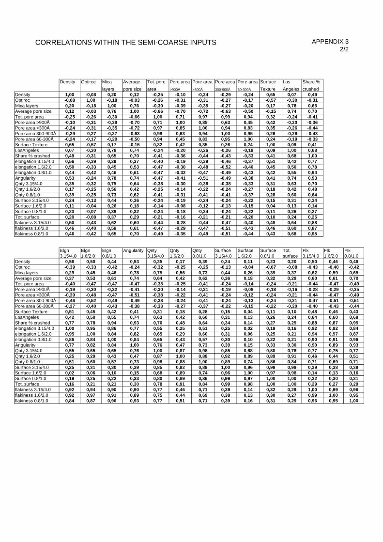
CORRELATIONS WITHIN THE SEMI-COARSE INPUTS APPENDIX 32/2
Density Optiroc Mica
layers
Average
pore size
Tot. pore
area
Pore area
>900Å
Pore area
>300Å
Pore area
300-900Å
Pore area
60-300Å
Surface
Texture
Los
Angeles
Share %
crushedDensity 1,00 -0,08 0,20 0,12 -0,25 -0,10 -0,24 -0,29 -0,24 0,65 0,07 0,49Optiroc -0,08 1,00 -0,18 -0,03 -0,26 -0,31 -0,31 -0,27 -0,17 -0,57 -0,30 -0,31Mica layers 0,20 -0,18 1,00 0,76 -0,30 -0,39 -0,35 -0,27 -0,20 0,17 0,78 0,65Average pore size 0,12 -0,03 0,76 1,00 -0,66 -0,70 -0,72 -0,63 -0,50 -0,15 0,74 0,70Tot. pore area -0,25 -0,26 -0,30 -0,66 1,00 0,71 0,97 0,99 0,94 0,32 -0,24 -0,41Pore area >900Å -0,10 -0,31 -0,39 -0,70 0,71 1,00 0,85 0,63 0,45 0,42 -0,20 -0,36Pore area >300Å -0,24 -0,31 -0,35 -0,72 0,97 0,85 1,00 0,94 0,83 0,35 -0,26 -0,44Pore area 300-900Å -0,29 -0,27 -0,27 -0,63 0,99 0,63 0,94 1,00 0,95 0,26 -0,26 -0,43Pore area 60-300Å -0,24 -0,17 -0,20 -0,50 0,94 0,45 0,83 0,95 1,00 0,24 -0,19 -0,33Surface Texture 0,65 -0,57 0,17 -0,15 0,32 0,42 0,35 0,26 0,24 1,00 0,09 0,41LosAngeles 0,07 -0,30 0,78 0,74 -0,24 -0,20 -0,26 -0,26 -0,19 0,09 1,00 0,68Share % crushed 0,49 -0,31 0,65 0,70 -0,41 -0,36 -0,44 -0,43 -0,33 0,41 0,68 1,00elongation 3.15/4.0 0,56 -0,39 0,29 0,37 -0,40 -0,19 -0,39 -0,46 -0,37 0,51 0,42 0,77elongation 1.6/2.0 0,50 -0,33 0,45 0,53 -0,47 -0,30 -0,48 -0,52 -0,40 0,45 0,50 0,78elongation 0.8/1.0 0,44 -0,42 0,46 0,61 -0,47 -0,32 -0,47 -0,49 -0,43 0,42 0,55 0,94Angularity 0,53 -0,24 0,78 0,74 -0,47 -0,41 -0,51 -0,49 -0,38 0,41 0,74 0,93Qnty 3.15/4.0 0,35 -0,32 0,75 0,64 -0,38 -0,30 -0,38 -0,38 -0,33 0,31 0,63 0,70Qnty 1.6/2.0 0,17 -0,25 0,56 0,42 -0,25 -0,14 -0,22 -0,24 -0,27 0,18 0,42 0,48Qnty 0.8/1.0 0,39 -0,25 0,73 0,62 -0,41 -0,31 -0,41 -0,41 -0,37 0,28 0,60 0,64Surface 3.15/4.0 0,24 -0,13 0,44 0,36 -0,24 -0,19 -0,24 -0,24 -0,22 0,15 0,31 0,34Surface 1.6/2.0 0,11 -0,04 0,26 0,18 -0,14 -0,08 -0,12 -0,13 -0,15 0,04 0,13 0,14Surface 0.8/1.0 0,23 -0,07 0,39 0,32 -0,24 -0,18 -0,24 -0,24 -0,22 0,11 0,26 0,27Tot. surface 0,20 -0,08 0,37 0,29 -0,21 -0,16 -0,21 -0,21 -0,20 0,10 0,24 0,25flakiness 3.15/4.0 0,50 -0,43 0,62 0,60 -0,44 -0,28 -0,44 -0,47 -0,40 0,48 0,64 0,88flakiness 1.6/2.0 0,46 -0,40 0,59 0,61 -0,47 -0,29 -0,47 -0,51 -0,43 0,46 0,60 0,87flakiness 0.8/1.0 0,46 -0,42 0,65 0,70 -0,49 -0,35 -0,49 -0,51 -0,44 0,43 0,68 0,95
Elgn 3.15/4.0
Elgn 1.6/2.0
Elgn 0.8/1.0
Angularity Qnty 3.15/4.0
Qnty 1.6/2.0
Qnty 0.8/1.0
Surface 3.15/4.0
Surface 1.6/2.0
Surface 0.8/1.0
Tot. surface
Flk 3.15/4.0
Flk 1.6/2.0
Flk 0.8/1.0
Density 0,56 0,50 0,44 0,53 0,35 0,17 0,39 0,24 0,11 0,23 0,20 0,50 0,46 0,46Optiroc -0,39 -0,33 -0,42 -0,24 -0,32 -0,25 -0,25 -0,13 -0,04 -0,07 -0,08 -0,43 -0,40 -0,42Mica layers 0,29 0,45 0,46 0,78 0,75 0,56 0,73 0,44 0,26 0,39 0,37 0,62 0,59 0,65Average pore size 0,37 0,53 0,61 0,74 0,64 0,42 0,62 0,36 0,18 0,32 0,29 0,60 0,61 0,70Tot. pore area -0,40 -0,47 -0,47 -0,47 -0,38 -0,25 -0,41 -0,24 -0,14 -0,24 -0,21 -0,44 -0,47 -0,49Pore area >900Å -0,19 -0,30 -0,32 -0,41 -0,30 -0,14 -0,31 -0,19 -0,08 -0,18 -0,16 -0,28 -0,29 -0,35Pore area >300Å -0,39 -0,48 -0,47 -0,51 -0,38 -0,22 -0,41 -0,24 -0,12 -0,24 -0,21 -0,44 -0,47 -0,49Pore area 300-900Å -0,46 -0,52 -0,49 -0,49 -0,38 -0,24 -0,41 -0,24 -0,13 -0,24 -0,21 -0,47 -0,51 -0,51Pore area 60-300Å -0,37 -0,40 -0,43 -0,38 -0,33 -0,27 -0,37 -0,22 -0,15 -0,22 -0,20 -0,40 -0,43 -0,44Surface Texture 0,51 0,45 0,42 0,41 0,31 0,18 0,28 0,15 0,04 0,11 0,10 0,48 0,46 0,43LosAngeles 0,42 0,50 0,55 0,74 0,63 0,42 0,60 0,31 0,13 0,26 0,24 0,64 0,60 0,68Share % crushed 0,77 0,78 0,94 0,93 0,70 0,48 0,64 0,34 0,14 0,27 0,25 0,88 0,87 0,95elongation 3.15/4.0 1,00 0,95 0,86 0,77 0,55 0,25 0,51 0,25 0,02 0,19 0,16 0,92 0,92 0,84elongation 1.6/2.0 0,95 1,00 0,84 0,82 0,65 0,29 0,60 0,31 0,06 0,25 0,21 0,94 0,97 0,87elongation 0.8/1.0 0,86 0,84 1,00 0,84 0,65 0,43 0,57 0,30 0,10 0,22 0,21 0,90 0,91 0,96Angularity 0,77 0,82 0,84 1,00 0,76 0,47 0,73 0,39 0,15 0,33 0,30 0,90 0,89 0,93Qnty 3.15/4.0 0,55 0,65 0,65 0,76 1,00 0,87 0,98 0,85 0,68 0,80 0,78 0,77 0,75 0,77Qnty 1.6/2.0 0,25 0,29 0,43 0,47 0,87 1,00 0,88 0,92 0,89 0,89 0,91 0,46 0,44 0,51Qnty 0.8/1.0 0,51 0,60 0,57 0,73 0,98 0,88 1,00 0,89 0,74 0,86 0,84 0,71 0,69 0,71Surface 3.15/4.0 0,25 0,31 0,30 0,39 0,85 0,92 0,89 1,00 0,96 0,99 0,99 0,39 0,38 0,39Surface 1.6/2.0 0,02 0,06 0,10 0,15 0,68 0,89 0,74 0,96 1,00 0,97 0,98 0,14 0,13 0,16Surface 0.8/1.0 0,19 0,25 0,22 0,33 0,80 0,89 0,86 0,99 0,97 1,00 1,00 0,32 0,30 0,31Tot. surface 0,16 0,21 0,21 0,30 0,78 0,91 0,84 0,99 0,98 1,00 1,00 0,29 0,27 0,29flakiness 3.15/4.0 0,92 0,94 0,90 0,90 0,77 0,46 0,71 0,39 0,14 0,32 0,29 1,00 0,99 0,96flakiness 1.6/2.0 0,92 0,97 0,91 0,89 0,75 0,44 0,69 0,38 0,13 0,30 0,27 0,99 1,00 0,95flakiness 0.8/1.0 0,84 0,87 0,96 0,93 0,77 0,51 0,71 0,39 0,16 0,31 0,29 0,96 0,95 1,00

APPENDIX 4 RELIABILITY OF THE SENSISTIVITY ANALYSIS –
FLOW VALUE, AIR %, BLEEDING AND COMPRESSIVE STRENGTHPAGE 1/14
Reliability of sensitivity analysis; SC- flakiness 3,15/4.0 mm-flow value
Reliability of sensitivity analysis; SC- angularity-flow value
Sensitivity analysis - difference between modelled and measured values
0
100
200
300
400
500
600
700
800
1.2 1.25 1.3 1.35 1.4 1.45
SC-Flkn 3.15/4.0 mm
Flo
w v
alu
e [m
m]
N30WR30AE30N35WR35AE35
Sensitivity analysis - difference between modelled and measured values
0
100
200
300
400
500
600
700
800
4.5 5 5.5 6 6.5 7 7.5 8 8.5 9
SC-Angularity
Flo
w v
alu
e [m
m]
N30W R30AE30N35W R35AE35

APPENDIX 4 RELIABILITY OF THE SENSISTIVITY ANALYSIS –
FLOW VALUE, AIR %, BLEEDING AND COMPRESSIVE STRENGTHPAGE 2/14
Reliability of sensitivity analysis; SC- elongation 3.15/4.0 mm-flow value
Reliability of sensitivity analysis; SC- pore area 300-900Å-flow value
Sensitivity analysis - difference between modelled and measured values
0
100
200
300
400
500
600
700
800
1.34 1.36 1.38 1.4 1.42 1.44 1.46 1.48
SC-Elgn 3.15/4.0 mm
Flo
w v
alu
e [m
m]
N30W R30AE30N35W R35AE35
Sensitivity analysis - difference between modelled and measured values
0
100
200
300
400
500
600
700
800
0 0.02 0.04 0.06 0.08 0.1 0.12 0.14
SC-pore area 300-900Å [m2/g]
Flo
w v
alu
e [m
m]
N30W R30AE30N35W R35AE35

APPENDIX 4 RELIABILITY OF THE SENSISTIVITY ANALYSIS –
FLOW VALUE, AIR %, BLEEDING AND COMPRESSIVE STRENGTHPAGE 3/14
Reliability of sensitivity analysis; SC- pore area >900Å-flow value
Reliability of sensitivity analysis; F- mica %-flow value
Sensitivity analysis - difference between modelled and measured values
0
100
200
300
400
500
600
700
800
0 0.02 0.04 0.06 0.08 0.1 0.12 0.14
SC-pore area>900Å [m2/g]
Flo
w v
alu
e [m
m]
N30W R30AE30N35W R35AE35
Sensitivity analysis - difference between modelled and measured values
0
100
200
300
400
500
600
700
800
0 2 4 6 8 10 12 14 16
F- mica %
Flo
w v
alu
e [m
m]
N30WR30AE30N35WR35AE35

APPENDIX 4 RELIABILITY OF THE SENSISTIVITY ANALYSIS –
FLOW VALUE, AIR %, BLEEDING AND COMPRESSIVE STRENGTHPAGE 4/14
Reliability of sensitivity analysis; F- Cu-flow value
Reliability of sensitivity analysis; F- BET value-flow value
Sensitivity analysis - difference between modelled and measured values
0
100
200
300
400
500
600
700
800
0 2 4 6 8 10 12 14 16 18
F - Cu
Flo
w v
alu
e [m
m]
N30WR30AE30N35WR35AE35
Sensitivity analysis - difference between modelled and measured values
0
100
200
300
400
500
600
700
800
0 2 4 6 8 10 12 14 16
F- BET [m2/g]
Flo
w v
alu
e [m
m]
N30WR30AE30N35WR35AE35

APPENDIX 4 RELIABILITY OF THE SENSISTIVITY ANALYSIS –
FLOW VALUE, AIR %, BLEEDING AND COMPRESSIVE STRENGTHPAGE 5/14
Reliability of sensitivity analysis; F- Zeta potential-flow value
Reliability of sensitivity analysis; SC- pore area 60-300Å-air %
Sensitivity analysis - difference between modelled and measured values
0
100
200
300
400
500
600
700
800
-20 -18 -16 -14 -12 -10 -8 -6 -4 -2 0
F - Zeta pot. [mV]
Flo
w v
alu
e [m
m]
N30WR30AE30N35WR35AE35
Sensitivity analysis - difference between modelled and measured values
0
1
2
3
4
5
6
7
8
0 0.02 0.04 0.06 0.08 0.1 0.12 0.14 0.16
SC-pore area 60-300Å [m2/g]
Air
%
N30WR30AE30N35WR35AE35

APPENDIX 4 RELIABILITY OF THE SENSISTIVITY ANALYSIS –
FLOW VALUE, AIR %, BLEEDING AND COMPRESSIVE STRENGTHPAGE 6/14
Reliability of sensitivity analysis; SC- pore area 300-900Å-air %
Reliability of sensitivity analysis; SC- flakiness 3.15/4.0 mm-air %
Sensitivity analysis - difference between modelled and measured values
0
1
2
3
4
5
6
7
8
0 0.02 0.04 0.06 0.08 0.1 0.12 0.14
SC-pore area 300-900Å [m2/g]
Air
%
N30WR30AE30N35WR35AE35
Sensitivity analysis - difference between modelled and measured values
0
1
2
3
4
5
6
7
8
1.2 1.25 1.3 1.35 1.4 1.45
SC-Flkn 3.15/4.0 mm
Air
%
N30WR30AE30N35WR35AE35

APPENDIX 4 RELIABILITY OF THE SENSISTIVITY ANALYSIS –
FLOW VALUE, AIR %, BLEEDING AND COMPRESSIVE STRENGTHPAGE 7/14
Reliability of sensitivity analysis; SC- angularity-air %
Reliability of sensitivity analysis; F- Cu-air %
Sensitivity analysis - difference between modelled and measured values
0
1
2
3
4
5
6
7
8
4.5 5 5.5 6 6.5 7 7.5 8 8.5 9
SC-Angularity
Air
%
N30WR30AE30N35WR35AE35
Sensitivity analysis - difference between modelled and measured values
0
1
2
3
4
5
6
7
8
2 4 6 8 10 12 14 16 18
F - Cu
Air
%
N30WR30AE30N35WR35AE35

APPENDIX 4 RELIABILITY OF THE SENSISTIVITY ANALYSIS –
FLOW VALUE, AIR %, BLEEDING AND COMPRESSIVE STRENGTHPAGE 8/14
Reliability of sensitivity analysis; F- BET value-air %
Reliability of sensitivity analysis; SC- total pore area-bleeding
Sensitivity analysis - difference between modelled and measured values
0
1
2
3
4
5
6
7
8
0 2 4 6 8 10 12 14 16
F- BET [m2/g]
Air
%
N30WR30AE30N35WR35AE35
Sensitivity analysis - difference between modelled and measured values
0
2
4
6
8
10
12
14
16
18
20
0 0.05 0.1 0.15 0.2 0.25 0.3 0.35 0.4
SC-tot. pore area [m2/g]
Ble
edin
g [
g/c
m3]
N30WR30AE30N35WR35AE35

APPENDIX 4 RELIABILITY OF THE SENSISTIVITY ANALYSIS –
FLOW VALUE, AIR %, BLEEDING AND COMPRESSIVE STRENGTHPAGE 9/14
Reliability of sensitivity analysis; SC- average pore size-bleeding
Reliability of sensitivity analysis; SC- elongation 0.8/1.0 mm-bleeding
Sensitivity analysis - difference between modelled and measured values
0
2
4
6
8
10
12
14
16
18
20
0 2 4 6 8 10 12
SC- avg.pore size [µm]
Ble
edin
g [
g/c
m3]
N30WR30AE30N35WR35AE35
Sensitivity analysis - difference between modelled and measured values
0
2
4
6
8
10
12
14
16
18
20
1.4 1.45 1.5 1.55 1.6 1.65 1.7
SC-Elgn 0.8/1.0 mm
Ble
edin
g [
g/c
m3]
N30WR30AE30N35WR35AE35

APPENDIX 4 RELIABILITY OF THE SENSISTIVITY ANALYSIS –
FLOW VALUE, AIR %, BLEEDING AND COMPRESSIVE STRENGTHPAGE 10/14
Reliability of sensitivity analysis; SC- flakiness 1.6/2.0 mm-bleeding
Reliability of sensitivity analysis; SC- elongation 1.6/2.0 mm-bleeding
Sensitivity analysis - difference between modelled and measured values
0
2
4
6
8
10
12
14
16
18
20
1.2 1.25 1.3 1.35 1.4 1.45 1.5
SC-Flkn 1.6/2.0 mm
Ble
edin
g [
g/c
m3]
N30WR30AE30N35WR35AE35
Sensitivity analysis - difference between modelled and measured values
0
2
4
6
8
10
12
14
16
18
20
1.3 1.35 1.4 1.45 1.5 1.55
SC-Elgn 1.6/2.0 mm
Ble
edin
g [
g/c
m3]
N30WR30AE30N35WR35AE35

APPENDIX 4 RELIABILITY OF THE SENSISTIVITY ANALYSIS –
FLOW VALUE, AIR %, BLEEDING AND COMPRESSIVE STRENGTHPAGE 11/14
Reliability of sensitivity analysis; F- BET value-bleeding
Reliability of sensitivity analysis; F- Zeta potential-bleeding
Sensitivity analysis - difference between modelled and measured values
0
2
4
6
8
10
12
14
16
18
20
0 2 4 6 8 10 12 14 16
F- BET [m2/g]
Ble
edin
g [
g/c
m3]
N30WR30AE30N35WR35AE35
Sensitivity analysis - difference between modelled and measured values
0
2
4
6
8
10
12
14
16
18
20
-20 -18 -16 -14 -12 -10 -8 -6 -4 -2 0
F - Zeta pot. [mV]
Ble
edin
g [
g/c
m3]
N30WR30AE30N35WR35AE35

APPENDIX 4 RELIABILITY OF THE SENSISTIVITY ANALYSIS –
FLOW VALUE, AIR %, BLEEDING AND COMPRESSIVE STRENGTHPAGE 12/14
Reliability of sensitivity analysis; F- density-bleeding
Reliability of sensitivity analysis; F- Cu-bleeding
Sensitivity analysis - difference between modelled and measured values
0
2
4
6
8
10
12
14
16
18
20
2.6 2.65 2.7 2.75 2.8 2.85 2.9 2.95 3 3.05
F- density [Mg/m3]
Ble
edin
g [
g/c
m3]
N30
WR30
AE30
N35WR35
AE35
Sensitivity analysis - difference between modelled and measured values
0
2
4
6
8
10
12
14
16
18
20
0 2 4 6 8 10 12 14 16 18
F - Cu
Ble
edin
g [
g/c
m3]
N30WR30AE30N35WR35AE35

APPENDIX 4 RELIABILITY OF THE SENSISTIVITY ANALYSIS –
FLOW VALUE, AIR %, BLEEDING AND COMPRESSIVE STRENGTHPAGE 13/14
Reliability of sensitivity analysis; SC- flakiness 3.15/4.0 mm-compressive strength
Reliability of sensitivity analysis; SC- quantity 1.6/2.0 mm-compressive strength
Sensitivity analysis - difference between modelled and measured values
35
40
45
50
55
60
65
70
1.2 1.25 1.3 1.35 1.4 1.45
SC-Flkn 3.15/4.0 mm
Co
mp
. Ste
ng
th [
MP
a]
N30WR30AE30N35WR35AE35
Sensitivity analysis - difference between modelled and measured values
35
40
45
50
55
60
65
70
14000000 15000000 16000000 17000000 18000000 19000000 20000000
SC-Qnty 1.6/2.0 mm
Co
mp
. Ste
ng
th [
MP
a]
N30WR30AE30N35WR35AE35

APPENDIX 4 RELIABILITY OF THE SENSISTIVITY ANALYSIS –
FLOW VALUE, AIR %, BLEEDING AND COMPRESSIVE STRENGTHPAGE 14/14
Reliability of sensitivity analysis; SC- Los Angeles value-compressive strength
Reliability of sensitivity analysis; SC- pore area 60-300Å-compressive strength
Sensitivity analysis - difference between modelled and measured values
35
40
45
50
55
60
65
70
20 22 24 26 28 30 32 34 36 38 40
SC-LA value (mod.) [%]
Co
mp
. Ste
ng
th [
MP
a]
N30WR30AE30N35WR35AE35
Sensitivity analysis - difference between modelled and measured vcalues
35
40
45
50
55
60
65
70
0 0.02 0.04 0.06 0.08 0.1 0.12 0.14 0.16
SC-pore area 60-300Å [m2/g]
Co
mp
. Ste
ng
th [
MP
a]
N30WR30AE30N35WR35AE35

INPUTS OF MODELLED AGGREGATE COMBINATIONS APPENDIX 5
SE
M
AE
WR
BE
T
F -
den
sity
[M
g/m
3]
F -
Zet
a p
ot.
[m
V]
F-
Cu
SC
- av
g. p
ore
siz
e [u
m]
SC
- to
t. p
ore
are
a [m
2/g
]
SC
- L
A v
alu
e (m
od
.) [
%]
SC
- E
lgn
3.1
5/4.
0 m
m
SC
- E
lgn
1.6
/2.0
mm
SC
- E
lgn
0.8
/1.0
mm
SC
- A
ng
ula
rity
SC
- Q
nty
1.6
/2.0
mm
SC
- F
lkn
3.1
5/4.
0 m
m
SC
- F
lkn
1.6
/2.0
mm
F-
Mic
a [%
]
SC
- P
ore
are
a >
900Å
[m
2/g
]
SC
- P
ore
are
a 30
0-90
0Å [
m2/
g]
SC
- P
ore
are
a 60
-300
Å [
m2/
g]
Past gravel 300 0 0 3,4 2,70 -9,1 8,8 1,77 0,08 21,5 1,36 1,36 1,46 4,9 17148914 1,25 1,25 6,00 0,03 0,04 0,01350 0 0 3,4 2,70 -9,1 8,8 1,77 0,08 21,5 1,36 1,36 1,46 4,9 15948490 1,25 1,25 6,00 0,03 0,04 0,01300 1 0 3,4 2,70 -9,1 8,8 1,77 0,08 21,5 1,36 1,36 1,46 4,9 15532017 1,25 1,25 6,00 0,03 0,04 0,01350 1 0 3,4 2,70 -9,1 8,8 1,77 0,08 21,5 1,36 1,36 1,46 4,9 16634447 1,25 1,25 6,00 0,03 0,04 0,01300 0 1 3,4 2,70 -15,1 8,8 1,77 0,08 21,5 1,36 1,36 1,46 4,9 17736877 1,25 1,25 6,00 0,03 0,04 0,01350 0 1 3,4 2,70 -15,1 8,8 1,77 0,08 21,5 1,36 1,36 1,46 4,9 16634447 1,25 1,25 6,00 0,03 0,04 0,01
Future gravel 300 0 0 9,3 2,71 -7,1 16,2 1,00 0,18 24,1 1,35 1,35 1,46 5,2 16991626 1,23 1,23 0,00 0,10 0,06 0,02350 0 0 9,3 2,71 -7,1 16,2 1,00 0,18 24,1 1,35 1,35 1,46 5,2 15802213 1,23 1,23 0,00 0,10 0,06 0,02300 1 0 9,3 2,71 -7,1 16,2 1,00 0,18 24,1 1,35 1,35 1,46 5,2 15389559 1,23 1,23 0,00 0,10 0,06 0,02350 1 0 9,3 2,71 -7,1 16,2 1,00 0,18 24,1 1,35 1,35 1,46 5,2 16481878 1,23 1,23 0,00 0,10 0,06 0,02300 0 1 9,3 2,71 -15,2 16,2 1,00 0,18 24,1 1,35 1,35 1,46 5,2 17574196 1,23 1,23 0,00 0,10 0,06 0,02350 0 1 9,3 2,71 -15,2 16,2 1,00 0,18 24,1 1,35 1,35 1,46 5,2 16481878 1,23 1,23 0,00 0,10 0,06 0,02
Good strenght&good shape 300 0 0 3,1 2,72 -8,8 10,7 7,62 0,02 19,6 1,41 1,46 1,59 7,1 17316121 1,33 1,34 6,00 0,02 0,00 0,00350 0 0 3,1 2,72 -8,8 10,7 7,62 0,02 19,6 1,41 1,46 1,59 7,1 16103993 1,33 1,34 6,00 0,02 0,00 0,00
Filler aggregate and 300 1 0 3,1 2,72 -8,8 10,7 7,62 0,02 19,6 1,41 1,46 1,59 7,1 15683459 1,33 1,34 6,00 0,02 0,00 0,00crushed rock 350 1 0 3,1 2,72 -8,8 10,7 7,62 0,02 19,6 1,41 1,46 1,59 7,1 16796638 1,33 1,34 6,00 0,02 0,00 0,00
300 0 1 3,1 2,72 -13,7 10,7 7,62 0,02 19,6 1,41 1,46 1,59 7,1 17909817 1,33 1,34 6,00 0,02 0,00 0,00350 0 1 3,1 2,72 -13,7 10,7 7,62 0,02 19,6 1,41 1,46 1,59 7,1 16796638 1,33 1,34 6,00 0,02 0,00 0,00
Good strength&poor shape 300 0 0 3,1 2,72 -8,8 10,7 7,62 0,02 19,6 1,43 1,51 1,57 8,6 18488322 1,43 1,42 6,00 0,02 0,00 0,00350 0 0 3,1 2,72 -8,8 10,7 7,62 0,02 19,6 1,43 1,51 1,57 8,6 17194139 1,43 1,42 6,00 0,02 0,00 0,00
Filler aggregate and 300 1 0 3,1 2,72 -8,8 10,7 7,62 0,02 19,6 1,43 1,51 1,57 8,6 16745137 1,43 1,42 6,00 0,02 0,00 0,00crushed rock 350 1 0 3,1 2,72 -8,8 10,7 7,62 0,02 19,6 1,43 1,51 1,57 8,6 17933672 1,43 1,42 6,00 0,02 0,00 0,00
300 0 1 3,1 2,72 -13,7 10,7 7,62 0,02 19,6 1,43 1,51 1,57 8,6 19122207 1,43 1,42 6,00 0,02 0,00 0,00350 0 1 3,1 2,72 -13,7 10,7 7,62 0,02 19,6 1,43 1,51 1,57 8,6 17933672 1,43 1,42 6,00 0,02 0,00 0,00
Poor strength&poor shape 300 0 0 3,1 2,72 -8,8 10,7 7,62 0,02 38,2 1,43 1,51 1,57 8,6 18488322 1,43 1,42 6,00 0,02 0,00 0,00350 0 0 3,1 2,72 -8,8 10,7 7,62 0,02 38,2 1,43 1,51 1,57 8,6 17194139 1,43 1,42 6,00 0,02 0,00 0,00
Filler aggregate and 300 1 0 3,1 2,72 -8,8 10,7 7,62 0,02 38,2 1,43 1,51 1,57 8,6 16745137 1,43 1,42 6,00 0,02 0,00 0,00crushed rock 350 1 0 3,1 2,72 -8,8 10,7 7,62 0,02 38,2 1,43 1,51 1,57 8,6 17933672 1,43 1,42 6,00 0,02 0,00 0,00
300 0 1 3,1 2,72 -13,7 10,7 7,62 0,02 38,2 1,43 1,51 1,57 8,6 19122207 1,43 1,42 6,00 0,02 0,00 0,00350 0 1 3,1 2,72 -13,7 10,7 7,62 0,02 38,2 1,43 1,51 1,57 8,6 17933672 1,43 1,42 6,00 0,02 0,00 0,00
Poor strength&good shape 300 0 0 3,1 2,72 -8,8 10,7 7,62 0,02 38,2 1,41 1,46 1,59 7,1 17316121 1,33 1,34 6,00 0,02 0,00 0,00350 0 0 3,1 2,72 -8,8 10,7 7,62 0,02 38,2 1,41 1,46 1,59 7,1 16103993 1,33 1,34 6,00 0,02 0,00 0,00
Filler aggregate and 300 1 0 3,1 2,72 -8,8 10,7 7,62 0,02 38,2 1,41 1,46 1,59 7,1 15683459 1,33 1,34 6,00 0,02 0,00 0,00crushed rock 350 1 0 3,1 2,72 -8,8 10,7 7,62 0,02 38,2 1,41 1,46 1,59 7,1 16796638 1,33 1,34 6,00 0,02 0,00 0,00
300 0 1 3,1 2,72 -13,7 10,7 7,62 0,02 38,2 1,41 1,46 1,59 7,1 17909817 1,33 1,34 6,00 0,02 0,00 0,00350 0 1 3,1 2,72 -13,7 10,7 7,62 0,02 38,2 1,41 1,46 1,59 7,1 16796638 1,33 1,34 6,00 0,02 0,00 0,00

N30 FLOW VALUE_COMBINED EFFECT APPENDIX 6A1/6
Testing data 300 0 0 3,12 2,718 -8,8 10,7 7,62 0,019 19,6 1,41 1,46 1,59 7,1 17316121 1,33 1,34 6 0,019 0 0stdev min max average
SC-Flkn 3.15/4.0 mm and SC-Pore area 300-900Å -> Flow value 49,6 304 470 364Surface 1,23 1,26 1,28 1,30 1,32 1,34 1,36 1,38 1,41 1,43
0,00 470 450 430 410 392 376 362 351 342 3370,01 470 448 425 403 383 365 350 339 331 3270,03 469 444 419 395 373 354 339 328 321 3180,04 466 439 412 386 363 344 329 319 313 3120,06 461 432 404 378 355 336 321 312 307 3070,07 454 425 396 370 347 329 316 307 304 3060,09 446 417 389 364 342 324 312 306 304 3070,10 438 410 383 359 338 322 312 307 307 3110,12 430 403 378 356 337 324 315 311 313 3180,13 423 398 376 355 339 327 321 319 321 327
41,1 39 218 103 6,9 5 33 15Difference between the 10% and 90% quantiles [MPa] Coefficient of variation for the expectation value [%]
81 68 59 50 42 39 40 46 55 68 8,6 7,6 6,8 6,1 5,4 5,2 5,5 6,5 8,1 10,087 73 62 53 46 42 43 48 56 68 9,3 8,2 7,3 6,6 6,0 5,8 6,1 7,1 8,5 10,496 81 69 60 56 54 55 60 68 80 10,2 9,1 8,2 7,6 7,5 7,6 8,2 9,1 10,6 12,5
105 89 77 70 66 66 70 76 85 98 11,2 10,1 9,4 9,1 9,1 9,6 10,6 11,9 13,6 15,7112 98 87 81 80 82 87 94 104 117 12,2 11,3 10,8 10,8 11,2 12,2 13,6 15,0 16,9 19,0121 106 97 93 93 97 103 113 126 139 13,4 12,5 12,3 12,5 13,4 14,8 16,4 18,4 20,6 22,8129 115 106 102 105 114 123 134 146 160 14,4 13,7 13,6 14,0 15,3 17,5 19,7 21,9 24,0 26,1136 123 114 113 119 126 137 151 165 182 15,5 14,9 14,9 15,8 17,6 19,5 22,0 24,6 26,8 29,2139 127 121 123 129 140 154 169 184 201 16,2 15,8 16,0 17,2 19,2 21,7 24,4 27,1 29,5 31,6146 134 130 133 142 155 170 185 201 218 17,3 16,8 17,3 18,7 20,9 23,6 26,4 29,1 31,3 33,3
stdev min max averageSC- Flkn 3.15/4.0 mm and F- Cu -> Flow value 45,4 332 489 394
Surface 1,23 1,26 1,28 1,30 1,32 1,34 1,36 1,38 1,41 1,433 489 468 448 427 407 390 374 362 352 3465 485 465 444 424 404 387 372 359 350 3446 482 461 441 421 401 384 369 357 348 3428 478 458 437 417 398 381 367 355 346 3409 474 454 434 414 395 379 364 353 344 339
11 470 450 430 410 392 376 362 351 342 33712 466 446 426 407 389 373 360 349 341 33614 462 442 423 404 386 371 357 347 339 33415 457 438 419 400 383 368 355 345 337 33316 453 434 415 397 380 365 353 343 336 332
13,6 38 89 57 1,5 5 11 7Difference between the 10% and 90% quantiles [MPa] Coefficient of variation for the expectation value [%]
89 77 67 59 53 50 51 55 63 73 9,1 8,2 7,5 6,9 6,5 6,5 6,8 7,6 8,9 10,587 74 63 56 49 46 47 51 59 69 9,0 8,0 7,1 6,6 6,1 6,0 6,3 7,1 8,4 10,186 73 62 53 47 44 44 48 57 68 8,9 7,9 7,0 6,3 5,8 5,7 5,9 6,8 8,1 9,985 72 61 52 45 41 41 46 55 67 8,9 7,8 6,9 6,2 5,6 5,4 5,6 6,5 8,0 9,883 70 59 50 43 40 40 46 54 66 8,7 7,7 6,8 6,1 5,5 5,3 5,5 6,5 7,9 9,782 69 58 49 42 38 39 45 54 67 8,7 7,7 6,7 5,9 5,3 5,1 5,4 6,4 7,9 10,081 67 57 48 41 38 40 46 55 68 8,7 7,5 6,6 5,9 5,3 5,1 5,6 6,6 8,1 10,180 67 57 48 42 39 41 47 57 70 8,7 7,6 6,8 6,0 5,4 5,3 5,7 6,8 8,4 10,480 67 57 48 43 41 43 50 60 73 8,8 7,7 6,8 6,0 5,6 5,6 6,1 7,2 8,9 10,981 69 58 50 45 43 45 52 62 76 9,0 7,9 7,0 6,3 5,9 5,8 6,4 7,6 9,3 11,5

N35 FLOW VALUE_COMBINED EFFECT APPENDIX 6A2/6
Testing data 350 0 0 3,12 2,718 -8,8 10,7 7,62 0,019 19,6 1,41 1,46 1,59 7,1 16103993 1,33 1,34 6 0,019 0 0stdev min max average
SC-Flkn 3.15/4.0 mm and SC-Pore area 300-900Å -> Flow value 43,4 421 570 491Surface 1,23 1,26 1,28 1,30 1,32 1,34 1,36 1,38 1,41 1,43
0,00 547 539 530 521 512 504 497 491 486 4830,01 555 544 532 519 508 497 488 481 476 4730,03 561 547 532 517 502 489 479 471 465 4620,04 566 550 532 514 497 482 469 460 454 4510,06 569 550 530 510 491 474 461 451 444 4410,07 570 550 528 506 485 467 453 442 436 4330,09 569 548 525 502 481 462 447 436 430 4270,10 566 545 522 499 477 459 443 432 426 4230,12 562 541 519 496 475 457 442 431 424 4210,13 556 536 515 494 474 456 442 432 425 422
39,0 35 206 96 4,7 3 24 10Difference between the 10% and 90% quantiles [MPa] Coefficient of variation for the expectation value [%]
70 58 47 39 35 35 38 45 54 66 6,4 5,3 4,4 3,8 3,4 3,5 3,8 4,5 5,5 6,976 62 52 45 41 39 41 46 55 66 6,8 5,7 4,9 4,4 4,0 3,9 4,2 4,8 5,8 7,084 71 60 54 51 50 52 58 65 76 7,5 6,5 5,7 5,2 5,1 5,1 5,5 6,1 7,0 8,295 80 71 66 63 64 67 72 81 91 8,3 7,3 6,7 6,4 6,4 6,6 7,1 7,9 8,9 10,1
104 91 82 77 76 79 83 90 99 109 9,1 8,3 7,7 7,6 7,8 8,3 9,1 10,0 11,2 12,3113 100 91 87 88 92 98 107 117 132 9,9 9,1 8,7 8,6 9,0 9,8 10,8 12,1 13,4 15,2123 109 101 98 101 107 115 125 135 148 10,8 10,0 9,6 9,8 10,5 11,6 12,9 14,4 15,7 17,4128 115 107 106 110 118 128 141 154 169 11,3 10,5 10,3 10,6 11,6 12,9 14,5 16,3 18,1 20,0134 121 116 117 122 132 144 157 169 185 12,0 11,2 11,1 11,8 12,9 14,5 16,3 18,2 19,9 21,9138 127 122 125 132 145 159 174 190 206 12,4 11,8 11,8 12,6 14,0 15,9 18,0 20,2 22,4 24,4
stdev min max averageSC- Flkn 3.15/4.0 mm and F- Cu -> Flow value 25,6 465 569 513
Surface 1,23 1,26 1,28 1,30 1,32 1,34 1,36 1,38 1,41 1,433 569 562 553 545 535 527 519 513 508 5035 565 558 549 540 531 523 515 509 504 5006 561 553 545 536 527 518 511 505 500 4968 556 549 540 531 522 514 506 500 495 4929 552 544 535 526 517 509 501 496 491 488
11 547 539 530 521 512 504 497 491 486 48312 542 534 525 516 507 499 492 486 482 47914 538 529 520 511 502 493 487 481 477 47415 533 524 515 505 496 488 481 476 472 47016 528 519 510 500 491 483 476 471 467 465
11,9 34 77 51 1,1 3 8 5Difference between the 10% and 90% quantiles [MPa] Coefficient of variation for the expectation value [%]
77 64 55 50 47 46 47 52 58 68 6,8 5,7 5,0 4,6 4,4 4,3 4,6 5,0 5,7 6,774 62 53 47 43 43 45 49 56 67 6,5 5,6 4,8 4,3 4,1 4,1 4,4 4,8 5,6 6,773 61 51 45 41 41 43 48 56 66 6,5 5,5 4,7 4,2 3,9 3,9 4,2 4,8 5,6 6,772 60 50 42 39 38 41 47 55 66 6,5 5,5 4,6 4,0 3,7 3,7 4,0 4,7 5,6 6,770 58 49 41 37 37 40 46 55 66 6,3 5,3 4,5 3,9 3,6 3,6 3,9 4,6 5,6 6,870 57 47 40 35 35 38 45 54 65 6,4 5,3 4,5 3,8 3,4 3,5 3,9 4,6 5,5 6,870 58 47 39 35 35 38 44 53 66 6,5 5,4 4,5 3,8 3,4 3,5 3,8 4,5 5,5 6,970 57 47 39 35 34 38 44 55 67 6,5 5,4 4,5 3,8 3,4 3,4 3,9 4,6 5,7 7,171 57 47 40 36 35 39 46 55 68 6,7 5,5 4,6 3,9 3,6 3,6 4,0 4,8 5,9 7,372 58 47 40 36 37 41 48 58 73 6,8 5,6 4,6 4,0 3,7 3,8 4,3 5,1 6,2 7,8

AE30 FLOW VALUE_COMBINED EFFECT APPENDIX 6A3/6
Testing data 300 1 0 3,12 2,718 -8,8 10,7 7,62 0,019 19,6 1,41 1,46 1,59 7,1 15683459 1,33 1,34 6 0,019 0 0stdev min max average
SC-Flkn 3.15/4.0 mm and SC-Pore area 300-900Å -> Flow value 45,4 268 427 322Surface 1,23 1,26 1,28 1,30 1,32 1,34 1,36 1,38 1,41 1,43
0,00 427 406 385 366 348 333 321 312 307 3050,01 425 401 378 356 336 320 308 299 295 2940,03 422 396 370 346 325 309 296 288 284 2850,04 418 389 362 337 315 298 286 279 276 2780,06 412 382 354 328 307 290 278 272 271 2750,07 405 375 347 321 300 284 273 268 269 2740,09 398 368 340 315 295 280 271 268 270 2770,10 391 362 336 312 293 280 273 271 275 2830,12 385 358 333 312 295 284 278 278 283 2920,13 380 355 333 314 299 290 286 288 294 303
42,2 38 230 103 7,8 6 38 16Difference between the 10% and 90% quantiles [MPa] Coefficient of variation for the expectation value [%]
82 69 58 48 42 38 40 47 57 71 9,6 8,5 7,5 6,6 6,0 5,8 6,2 7,5 9,3 11,688 73 61 52 44 40 41 47 57 71 10,3 9,1 8,1 7,2 6,6 6,2 6,7 7,8 9,7 12,296 81 68 58 51 49 52 59 69 84 11,4 10,2 9,2 8,4 7,9 8,0 8,8 10,3 12,2 14,8
105 89 77 68 63 63 67 76 87 102 12,6 11,5 10,7 10,0 10,0 10,5 11,7 13,6 15,7 18,3113 97 85 77 75 79 86 93 105 122 13,7 12,7 12,0 11,8 12,2 13,7 15,4 17,1 19,4 22,3120 104 93 88 88 93 102 114 127 143 14,8 13,9 13,5 13,7 14,8 16,5 18,7 21,2 23,6 26,1127 111 101 99 101 108 119 133 149 167 15,9 15,1 14,9 15,7 17,0 19,3 22,0 24,9 27,6 30,1134 119 110 109 115 124 135 150 167 185 17,1 16,4 16,4 17,4 19,5 22,1 24,7 27,7 30,4 32,7138 123 117 118 126 138 152 170 188 207 17,9 17,2 17,5 19,0 21,3 24,3 27,4 30,5 33,2 35,5143 131 126 130 140 154 170 187 207 230 18,8 18,4 19,0 20,7 23,4 26,6 29,7 32,5 35,3 37,9
stdev min max averageSC- Flkn 3.15/4.0 mm and F- Cu -> Flow value 42,6 302 449 353
Surface 1,23 1,26 1,28 1,30 1,32 1,34 1,36 1,38 1,41 1,433 449 427 405 384 364 347 333 323 316 3135 444 423 401 380 361 344 331 320 314 3116 440 419 397 376 358 341 328 318 312 3098 436 414 393 373 354 338 326 316 310 3089 431 410 389 369 351 336 323 314 308 306
11 427 406 385 366 348 333 321 312 307 30512 423 402 381 362 345 330 319 310 305 30414 418 398 377 359 342 328 317 309 304 30315 414 393 374 355 339 326 315 307 303 30216 410 389 370 352 337 324 313 306 302 302
14,4 37 92 58 1,8 6 13 8Difference between the 10% and 90% quantiles [MPa] Coefficient of variation for the expectation value [%]
92 81 70 60 55 53 54 58 66 77 10,2 9,5 8,6 7,8 7,5 7,6 8,1 9,0 10,4 12,291 77 66 57 51 49 50 54 62 73 10,2 9,1 8,2 7,5 7,1 7,1 7,5 8,4 9,9 11,788 76 64 55 48 45 45 50 59 70 10,0 9,0 8,1 7,3 6,7 6,5 6,9 7,9 9,4 11,486 73 61 52 45 42 43 48 57 70 9,9 8,8 7,8 7,0 6,4 6,2 6,6 7,6 9,2 11,485 71 59 49 43 40 41 47 56 69 9,9 8,7 7,5 6,7 6,2 5,9 6,4 7,4 9,2 11,382 68 57 48 41 38 40 46 57 71 9,6 8,4 7,4 6,6 5,9 5,7 6,2 7,4 9,4 11,781 67 56 47 41 37 40 47 58 71 9,6 8,4 7,4 6,5 5,9 5,7 6,2 7,6 9,5 11,780 66 55 46 40 38 41 49 60 74 9,6 8,4 7,3 6,4 5,9 5,8 6,5 7,9 9,8 12,380 67 55 46 40 40 43 51 63 77 9,7 8,5 7,4 6,5 6,0 6,1 6,8 8,3 10,4 12,881 67 56 48 43 41 46 54 66 80 9,9 8,7 7,6 6,8 6,3 6,4 7,3 8,8 10,8 13,3

AE35 FLOW VALUE_COMBINED EFFECT APPENDIX 6A4/6
Testing data 350 1 0 3,12 2,718 -8,8 10,7 7,62 0,019 19,6 1,41 1,46 1,59 7,1 16796638 1,33 1,34 6 0,019 0 0stdev min max average
SC-Flkn 3.15/4.0 mm and SC-Pore area 300-900Å -> Flow value 38,6 377 503 432Surface 1,23 1,26 1,28 1,30 1,32 1,34 1,36 1,38 1,41 1,43
0,00 493 483 474 464 454 446 439 434 431 4290,01 497 485 472 459 447 437 429 423 419 4190,03 500 485 469 454 440 428 418 412 408 4080,04 502 485 467 449 433 419 409 402 398 3980,06 503 483 463 444 426 411 400 393 389 3900,07 502 481 460 439 420 405 393 386 383 3830,09 500 479 457 435 416 400 389 381 379 3800,10 497 476 454 432 414 398 387 380 377 3790,12 494 473 451 431 413 398 387 381 379 3800,13 490 470 450 431 414 400 390 385 383 384
39,5 37 210 98 5,3 4 27 12Difference between the 10% and 90% quantiles [MPa] Coefficient of variation for the expectation value [%]
72 60 50 43 38 37 38 44 52 65 7,3 6,2 5,3 4,6 4,2 4,1 4,4 5,1 6,1 7,578 65 55 48 43 40 41 46 54 65 7,9 6,7 5,8 5,2 4,8 4,5 4,8 5,4 6,4 7,886 73 64 57 52 50 51 56 63 75 8,6 7,6 6,8 6,3 5,9 5,9 6,1 6,8 7,8 9,297 84 74 67 64 64 66 71 79 91 9,6 8,6 7,9 7,5 7,4 7,6 8,1 8,8 9,9 11,4
106 93 84 78 76 77 81 89 98 110 10,5 9,6 9,1 8,8 8,9 9,4 10,2 11,4 12,6 14,1114 101 93 89 89 92 98 107 117 130 11,3 10,5 10,1 10,1 10,6 11,4 12,5 13,9 15,2 16,9122 110 102 99 101 106 115 125 137 152 12,2 11,5 11,2 11,4 12,1 13,3 14,8 16,4 18,1 20,0129 117 109 108 113 121 132 143 157 172 13,0 12,3 12,1 12,5 13,7 15,2 17,0 18,8 20,8 22,7133 123 117 118 123 133 144 158 174 191 13,5 13,0 13,0 13,7 14,9 16,7 18,6 20,7 23,0 25,1136 126 124 128 136 147 160 176 192 210 13,9 13,4 13,7 14,8 16,5 18,3 20,5 22,9 25,1 27,3
stdev min max averageSC- Flkn 3.15/4.0 mm and F- Cu -> Flow value 25,4 414 516 457
Surface 1,23 1,26 1,28 1,30 1,32 1,34 1,36 1,38 1,41 1,433 516 507 497 487 477 469 461 455 451 4485 511 502 493 483 473 464 457 451 447 4456 507 498 488 478 468 460 452 447 443 4418 502 493 483 473 464 455 448 442 439 4379 498 488 478 468 459 450 443 438 435 433
11 493 484 474 464 454 446 439 434 431 42912 488 479 469 459 449 441 434 429 426 42514 483 474 464 454 445 437 430 425 422 42215 479 469 459 449 440 432 426 421 418 41816 474 465 455 445 436 428 421 417 415 414
11,8 35 80 52 1,2 4 8 6Difference between the 10% and 90% quantiles [MPa] Coefficient of variation for the expectation value [%]
80 69 60 53 49 48 48 51 56 66 7,8 6,8 6,0 5,5 5,2 5,1 5,2 5,6 6,3 7,478 66 57 51 46 45 46 49 56 65 7,7 6,6 5,8 5,2 4,9 4,8 5,0 5,4 6,3 7,475 63 54 47 43 42 43 48 55 65 7,4 6,4 5,5 5,0 4,6 4,6 4,8 5,4 6,2 7,473 61 53 46 41 40 41 45 53 64 7,3 6,2 5,4 4,8 4,4 4,3 4,6 5,1 6,1 7,373 61 51 43 39 38 40 45 53 65 7,3 6,3 5,4 4,6 4,2 4,2 4,5 5,1 6,1 7,472 60 50 42 38 36 38 44 53 64 7,3 6,2 5,3 4,6 4,1 4,1 4,4 5,1 6,1 7,571 59 49 42 37 35 38 44 53 65 7,3 6,2 5,3 4,6 4,1 4,0 4,4 5,1 6,2 7,672 59 49 41 36 35 38 44 53 66 7,4 6,2 5,3 4,5 4,1 4,0 4,4 5,2 6,3 7,872 59 49 41 37 36 39 45 55 67 7,5 6,3 5,3 4,6 4,2 4,2 4,6 5,4 6,5 8,172 59 49 42 38 37 41 48 58 70 7,6 6,4 5,4 4,7 4,3 4,4 4,9 5,7 6,9 8,5

WR30 FLOW VALUE_COMBINED EFFECT APPENDIX 6A5/6
Testing data 300 0 1 3,12 2,718 -13,7 10,7 7,62 0,019 19,6 1,41 1,46 1,59 7,1 17909817 1,33 1,34 6 0,019 0 0stdev min max average
SC-Flkn 3.15/4.0 mm and SC-Pore area 300-900Å -> Flow value 63,6 306 535 382Surface 1,23 1,26 1,28 1,30 1,32 1,34 1,36 1,38 1,41 1,43
0,00 535 511 485 458 431 407 384 366 351 3410,01 530 503 474 446 418 392 370 352 338 3290,03 521 492 462 432 403 378 356 339 326 3190,04 510 480 449 418 389 364 343 328 317 3120,06 497 466 435 404 376 352 333 319 310 3070,07 482 452 421 391 365 343 325 313 307 3060,09 468 438 408 381 356 336 321 311 307 3080,10 454 426 398 372 350 332 320 312 310 3130,12 442 416 390 367 348 332 322 317 317 3210,13 431 408 385 365 348 336 328 325 326 331
44,1 40 233 110 7,5 5 35 15Difference between the 10% and 90% quantiles [MPa] Coefficient of variation for the expectation value [%]
83 69 58 48 42 40 42 49 58 70 7,7 6,8 5,9 5,2 4,8 4,9 5,5 6,7 8,3 10,389 75 63 54 47 44 46 52 60 72 8,4 7,5 6,7 6,0 5,6 5,6 6,2 7,3 8,9 10,998 83 72 64 59 57 59 65 73 84 9,5 8,5 7,8 7,4 7,3 7,6 8,3 9,5 11,2 13,2
110 96 83 76 73 73 76 83 92 103 10,8 10,0 9,3 9,1 9,3 10,0 11,1 12,7 14,5 16,6118 104 94 88 87 89 96 104 111 123 11,8 11,1 10,8 10,9 11,5 12,7 14,5 16,3 17,9 20,1127 114 105 100 102 106 113 124 135 149 13,2 12,6 12,5 12,8 14,0 15,5 17,4 19,8 22,1 24,3134 121 113 112 115 121 131 143 156 170 14,3 13,8 13,8 14,7 16,1 18,1 20,5 23,0 25,4 27,6139 129 122 122 128 138 150 163 176 192 15,4 15,1 15,3 16,4 18,3 20,8 23,4 26,1 28,3 30,7145 134 129 132 141 152 165 181 197 215 16,5 16,1 16,6 18,0 20,2 22,9 25,6 28,5 31,1 33,6148 137 135 141 152 166 182 198 216 233 17,2 16,8 17,5 19,2 21,7 24,7 27,7 30,5 33,1 35,2
stdev min max averageSC- Flkn 3.15/4.0 mm and F- Cu -> Flow value 66,0 331 551 428
Surface 1,23 1,26 1,28 1,30 1,32 1,34 1,36 1,38 1,41 1,433 551 528 503 476 450 424 401 382 365 3545 549 525 500 473 446 421 398 378 363 3516 546 522 496 470 443 418 395 375 360 3488 543 519 493 466 439 414 391 372 357 3469 539 515 489 462 435 410 388 369 354 343
11 535 511 485 458 431 407 384 366 351 34112 531 507 481 454 427 403 381 362 348 33814 527 502 476 449 423 399 377 359 345 33615 522 498 471 445 419 395 373 356 342 33416 517 493 467 440 414 390 370 353 340 331
13,7 39 89 58 1,7 5 12 7Difference between the 10% and 90% quantiles [MPa] Coefficient of variation for the expectation value [%]
89 77 68 60 54 52 52 55 61 70 8,1 7,3 6,8 6,3 6,0 6,1 6,4 7,2 8,4 9,988 75 65 57 51 47 48 51 58 67 8,0 7,2 6,5 6,0 5,7 5,6 6,0 6,8 8,0 9,688 75 64 54 48 44 45 50 57 67 8,0 7,2 6,4 5,8 5,4 5,3 5,7 6,6 8,0 9,686 73 61 52 46 42 43 48 56 67 7,9 7,0 6,2 5,6 5,2 5,1 5,5 6,5 7,9 9,784 71 59 50 43 41 43 49 57 68 7,8 6,9 6,1 5,4 5,0 5,0 5,5 6,7 8,1 9,984 70 57 48 42 40 42 48 58 70 7,8 6,8 5,9 5,2 4,9 4,9 5,5 6,6 8,2 10,383 68 56 47 41 39 42 49 59 71 7,8 6,7 5,9 5,1 4,8 4,8 5,5 6,8 8,5 10,581 67 55 46 40 39 44 51 62 74 7,7 6,6 5,8 5,1 4,7 4,9 5,8 7,1 8,9 11,181 67 55 46 42 41 47 55 65 77 7,8 6,7 5,9 5,2 5,0 5,2 6,2 7,7 9,5 11,682 68 56 48 44 44 50 59 70 82 7,9 6,9 6,0 5,5 5,3 5,7 6,8 8,3 10,2 12,4

WR35 FLOW VALUE_COMBINED EFFECT APPENDIX 6A6/6
Testing data 350 0 1 3,12 2,718 -13,7 10,7 7,62 0,019 19,6 1,41 1,46 1,59 7,1 16796638 1,33 1,34 6 0,019 0 0stdev min max average
SC-Flkn 3.15/4.0 mm and SC-Pore area 300-900Å -> Flow value 66,9 459 700 588Surface 1,23 1,26 1,28 1,30 1,32 1,34 1,36 1,38 1,41 1,43
0,00 699 696 689 681 671 660 649 638 627 6150,01 700 693 683 671 659 646 634 622 610 5990,03 695 685 672 658 643 628 615 602 590 5800,04 686 673 657 641 624 607 593 580 568 5590,06 673 658 640 621 602 585 570 557 546 5370,07 657 640 621 600 581 563 547 534 524 5160,09 640 621 601 580 560 541 526 513 504 4970,10 621 602 581 560 540 522 507 496 487 4810,12 601 583 563 543 523 506 492 481 473 4680,13 582 565 546 527 509 493 480 470 463 459
41,1 39 216 106 4,7 3 24 10Difference between the 10% and 90% quantiles [MPa] Coefficient of variation for the expectation value [%]
81 68 57 48 42 39 40 47 57 70 5,8 4,9 4,1 3,5 3,1 2,9 3,1 3,7 4,6 5,785 72 62 54 47 44 45 50 58 70 6,1 5,2 4,6 4,0 3,6 3,4 3,5 4,0 4,8 5,893 82 72 64 60 58 59 63 70 79 6,7 6,0 5,3 4,9 4,7 4,6 4,8 5,2 5,9 6,8
102 91 83 76 73 73 76 80 87 96 7,4 6,8 6,3 5,9 5,9 6,0 6,4 6,9 7,6 8,6111 100 93 88 87 89 93 100 108 118 8,3 7,6 7,2 7,1 7,2 7,6 8,2 9,0 9,9 11,0120 109 103 100 102 106 112 120 129 138 9,1 8,5 8,3 8,4 8,8 9,4 10,2 11,2 12,3 13,4128 119 113 111 114 121 129 139 149 161 10,0 9,6 9,4 9,6 10,2 11,1 12,3 13,5 14,8 16,2136 126 120 121 124 133 142 156 168 180 10,9 10,5 10,3 10,8 11,5 12,7 14,0 15,7 17,3 18,7140 128 125 127 135 146 159 173 186 200 11,6 11,0 11,1 11,7 12,9 14,4 16,2 18,0 19,6 21,4144 135 134 137 146 159 172 188 203 216 12,4 12,0 12,2 13,0 14,4 16,1 17,9 20,0 21,9 23,6
stdev min max averageSC- Flkn 3.15/4.0 mm and F- Cu -> Flow value 31,8 586 710 663
Surface 1,23 1,26 1,28 1,30 1,32 1,34 1,36 1,38 1,41 1,433 710 709 706 700 693 684 675 664 653 6405 709 707 703 697 690 681 671 660 649 6366 707 705 701 694 686 677 667 656 644 6328 705 703 698 690 682 672 661 650 639 6279 703 699 694 686 677 666 656 644 633 621
11 699 696 689 681 671 660 649 638 627 61512 696 691 684 675 665 654 643 631 620 60814 691 686 679 669 658 647 635 624 612 60115 687 681 673 662 651 639 628 616 605 59416 682 675 666 655 644 632 620 608 597 586
13,6 38 87 58 1,0 3 7 4Difference between the 10% and 90% quantiles [MPa] Coefficient of variation for the expectation value [%]
87 75 65 56 50 47 47 50 56 65 6,1 5,3 4,6 4,0 3,6 3,4 3,5 3,7 4,3 5,185 72 62 54 48 45 45 49 56 65 6,0 5,1 4,4 3,9 3,5 3,3 3,3 3,7 4,3 5,184 71 61 52 45 43 44 49 56 66 5,9 5,0 4,3 3,7 3,3 3,2 3,3 3,7 4,3 5,382 69 59 50 44 42 43 48 56 67 5,8 4,9 4,2 3,7 3,3 3,1 3,2 3,7 4,4 5,482 69 58 49 43 40 41 47 56 68 5,8 4,9 4,2 3,6 3,2 3,0 3,2 3,6 4,4 5,581 68 57 48 41 38 40 47 57 70 5,8 4,9 4,2 3,5 3,1 2,9 3,1 3,7 4,6 5,780 68 57 48 41 38 40 48 59 72 5,8 4,9 4,2 3,5 3,1 2,9 3,1 3,8 4,7 6,081 68 57 49 42 40 43 51 62 75 5,8 5,0 4,2 3,6 3,2 3,1 3,3 4,1 5,0 6,283 70 59 51 45 43 47 56 66 79 6,0 5,1 4,4 3,8 3,4 3,4 3,8 4,5 5,4 6,785 72 62 54 50 49 53 62 74 87 6,2 5,3 4,7 4,1 3,9 3,9 4,3 5,1 6,2 7,4

AE30 AIR % _ COMBINED EFFECT APPENDIX 6B1/2
Testing data 300 1 0 3,12125 2,718175 -8,78 10,675 7,62 0,0185 19,6 1,414225 1,459034 1,587608 7,100297 15683459 1,327366 1,343331 6 0,0185 0 0stdev min max average
SC- Flkn 3.15/4.0 mm and SC- Pore area 60-300Å -> Air % 1,0 2 5 3Surface 1,23 1,26 1,28 1,30 1,32 1,34 1,36 1,38 1,41 1,43
0,00 5,1 4,9 4,7 4,6 4,4 4,3 4,2 4,1 4,1 4,00,02 4,9 4,6 4,4 4,2 4,1 3,9 3,8 3,7 3,7 3,60,03 3,9 3,7 3,6 3,4 3,3 3,2 3,1 3,0 3,0 3,00,05 2,9 2,8 2,7 2,6 2,5 2,4 2,4 2,3 2,3 2,30,06 2,3 2,2 2,1 2,0 2,0 2,0 1,9 1,9 1,9 1,90,08 2,0 1,9 1,9 1,8 1,8 1,8 1,8 1,8 1,8 1,80,10 1,9 1,9 1,9 1,8 1,8 1,8 1,8 1,8 1,8 1,80,11 2,1 2,0 2,0 2,0 2,0 1,9 1,9 1,9 1,9 1,90,13 2,2 2,2 2,2 2,2 2,1 2,1 2,1 2,0 2,0 2,00,14 2,3 2,3 2,3 2,3 2,3 2,2 2,2 2,1 2,1 2,1
1,0 1 4 3 33,1 13 111 69Difference between the 10% and 90% quantiles [MPa] Coefficient of variation for the expectation value [%]
2,9 2,4 2,0 1,7 1,4 1,2 1,1 1,1 1,2 1,4 27,9 24,7 21,2 18,4 15,8 13,7 12,8 13,0 14,4 16,92,8 2,5 2,2 2,0 1,9 1,9 2,0 2,1 2,3 2,5 29,1 26,5 24,5 23,6 23,9 24,5 26,1 28,6 31,2 33,93,0 2,7 2,4 2,2 2,1 2,0 2,1 2,2 2,3 2,5 39,0 36,2 33,8 32,3 31,6 32,0 33,4 35,8 38,9 42,02,9 2,7 2,5 2,3 2,2 2,2 2,2 2,3 2,4 2,6 50,3 48,7 47,0 45,2 44,9 45,5 46,8 48,9 51,7 54,92,9 2,8 2,7 2,6 2,6 2,6 2,6 2,7 2,8 2,9 64,8 64,1 63,8 64,5 65,5 66,3 68,2 69,8 72,1 74,63,3 3,2 3,2 3,1 3,1 3,1 3,1 3,2 3,3 3,3 83,6 83,7 84,3 85,5 85,7 87,4 89,2 91,7 93,3 94,43,8 3,8 3,7 3,7 3,6 3,7 3,6 3,7 3,8 3,8 97,1 99,2 99,9 100,9 100,4 101,8 102,3 103,3 106,5 107,24,2 4,2 4,2 4,0 4,0 4,0 4,0 4,0 4,1 4,1 101,8 102,2 102,8 101,5 102,6 104,1 105,5 106,9 110,1 111,04,4 4,3 4,3 4,3 4,3 4,3 4,3 4,5 4,5 4,3 97,6 97,7 98,3 99,5 100,9 102,9 104,6 109,2 110,9 108,64,4 4,4 4,4 4,4 4,4 4,4 4,5 4,5 4,5 4,4 93,2 93,3 95,5 96,6 97,2 99,1 101,9 104,2 106,3 107,1
stdev min max averageF- Cu and SC- Pore area 60-300Å -> Air % 0,9 2 5 3
Surface 3,39 4,85 6,30 7,76 9,21 10,67 12,12 13,58 15,03 16,480,00 4,7 4,7 4,6 4,5 4,4 4,4 4,3 4,2 4,1 4,00,02 4,5 4,4 4,3 4,2 4,1 4,0 3,9 3,8 3,7 3,70,03 3,6 3,5 3,5 3,4 3,3 3,2 3,1 3,1 3,0 2,90,05 2,8 2,7 2,6 2,6 2,5 2,5 2,4 2,3 2,3 2,30,06 2,2 2,1 2,1 2,1 2,0 2,0 1,9 1,9 1,9 1,80,08 1,9 1,9 1,9 1,8 1,8 1,8 1,8 1,7 1,7 1,70,10 1,9 1,9 1,9 1,9 1,8 1,8 1,8 1,8 1,7 1,70,11 2,1 2,1 2,0 2,0 2,0 2,0 1,9 1,9 1,9 1,90,13 2,3 2,2 2,2 2,2 2,2 2,1 2,1 2,1 2,1 2,00,14 2,4 2,4 2,3 2,3 2,3 2,3 2,2 2,2 2,2 2,1
1,0 1 5 3 33,5 15 108 68Difference between the 10% and 90% quantiles [MPa] Coefficient of variation for the expectation value [%]
1,7 1,6 1,5 1,4 1,3 1,3 1,3 1,2 1,2 1,3 17,5 16,8 16,2 15,5 15,1 14,9 14,8 14,8 15,1 15,62,5 2,4 2,3 2,1 2,0 1,9 1,9 1,8 1,8 1,8 28,5 27,3 26,3 25,5 24,6 24,0 23,7 23,6 23,7 24,32,6 2,5 2,3 2,2 2,1 2,0 2,0 1,9 1,9 1,9 36,5 35,2 33,1 32,2 32,2 31,8 31,3 31,4 31,8 32,82,6 2,5 2,4 2,3 2,2 2,2 2,1 2,1 2,1 2,1 46,5 45,6 45,1 44,6 44,5 44,5 44,8 45,2 46,2 46,92,8 2,8 2,7 2,6 2,6 2,6 2,6 2,6 2,6 2,6 64,3 64,4 64,7 63,7 64,4 65,7 66,6 67,9 68,9 70,13,2 3,2 3,2 3,1 3,1 3,1 3,1 3,0 3,1 3,1 83,3 83,9 84,4 85,2 85,1 86,3 87,5 87,9 89,2 92,73,8 3,7 3,7 3,7 3,7 3,7 3,6 3,6 3,6 3,6 97,9 97,3 98,2 98,9 100,3 101,1 101,6 102,6 103,8 104,74,2 4,2 4,2 4,2 4,2 4,1 4,0 4,0 4,1 4,0 101,2 102,0 102,3 105,7 106,1 103,5 103,9 104,5 107,6 108,34,5 4,5 4,4 4,4 4,3 4,3 4,3 4,2 4,2 4,2 100,9 100,9 99,9 100,0 100,4 100,7 101,0 101,9 102,3 103,24,7 4,6 4,6 4,6 4,4 4,4 4,4 4,4 4,3 4,2 98,5 98,3 98,9 98,8 97,3 97,4 99,4 99,6 99,7 98,9

AE35 AIR % _ COMBINED EFFECT APPENDIX 6B2/2
Testing data 350 1 0 3,12125 2,718175 -8,78 10,675 7,62 0,0185 19,6 1,414225 1,459034 1,587608 7,100297 16796638 1,327366 1,343331 6 0,0185 0 0stdev min max average
SC- Flkn 3.15/4.0 mm and SC- Pore area 60-300Å -> Air % 1,2 2 7 3Surface 1,23 1,26 1,28 1,30 1,32 1,34 1,36 1,38 1,41 1,43
0,00 4,5 4,8 5,0 5,3 5,6 5,9 6,2 6,4 6,6 6,60,02 4,2 4,4 4,6 4,8 5,1 5,4 5,6 5,8 6,0 6,00,03 3,5 3,7 3,8 4,0 4,1 4,3 4,5 4,6 4,7 4,80,05 2,9 3,0 3,1 3,1 3,2 3,3 3,4 3,5 3,6 3,60,06 2,5 2,5 2,6 2,6 2,7 2,7 2,8 2,8 2,8 2,80,08 2,4 2,4 2,4 2,4 2,4 2,4 2,4 2,4 2,4 2,40,10 2,5 2,5 2,5 2,4 2,4 2,4 2,4 2,4 2,3 2,30,11 2,7 2,7 2,7 2,6 2,6 2,5 2,5 2,4 2,4 2,30,13 2,9 2,9 2,9 2,8 2,8 2,7 2,6 2,5 2,4 2,30,14 3,0 3,0 3,0 2,9 2,8 2,8 2,7 2,6 2,5 2,4
1,3 1 6 4 32,4 11 112 67Difference between the 10% and 90% quantiles [MPa] Coefficient of variation for the expectation value [%]
2,3 2,1 1,8 1,6 1,5 1,4 1,4 1,5 1,6 1,9 25,8 21,7 17,8 14,9 13,2 12,0 11,3 11,4 12,3 14,52,4 2,2 2,1 2,0 2,0 2,1 2,3 2,6 2,9 3,2 28,3 25,4 22,6 20,4 19,4 19,5 20,4 22,0 24,0 26,72,9 2,7 2,5 2,4 2,3 2,4 2,6 2,8 3,1 3,5 41,2 37,1 33,4 29,9 27,9 27,8 28,5 30,3 33,2 36,63,4 3,3 3,2 3,1 3,0 3,0 3,1 3,3 3,5 3,8 58,3 54,7 51,6 48,7 46,1 44,9 45,1 46,4 48,7 51,83,7 3,7 3,7 3,6 3,6 3,6 3,7 3,9 3,9 4,1 74,1 72,6 70,7 69,0 66,6 66,2 67,6 69,0 69,4 71,73,9 4,0 3,9 3,9 3,9 4,0 4,1 4,1 4,2 4,2 82,8 82,8 81,8 79,7 79,8 82,4 83,1 84,4 85,0 87,14,5 4,5 4,5 4,5 4,5 4,4 4,4 4,4 4,4 4,5 91,9 91,0 91,6 91,8 92,2 90,6 91,8 92,5 94,1 98,85,1 5,1 5,0 4,9 5,0 4,9 4,8 4,8 4,8 4,7 95,5 95,0 93,8 94,1 96,1 97,5 97,5 99,3 101,4 102,75,4 5,5 5,4 5,5 5,5 5,4 5,3 5,2 5,1 5,0 94,1 94,7 94,8 97,9 99,5 101,4 101,6 104,2 104,9 107,45,7 5,7 5,7 5,7 5,7 5,6 5,5 5,4 5,4 5,3 96,2 96,0 96,5 98,4 100,1 101,6 104,1 106,1 108,8 112,0
stdev min max averageF- Cu and SC- Pore area 60-300Å -> Air % 1,2 2 6 3
Surface 3,39 4,85 6,30 7,76 9,21 10,67 12,12 13,58 15,03 16,480,00 5,9 5,9 5,8 5,8 5,7 5,7 5,6 5,6 5,5 5,40,02 5,5 5,4 5,4 5,3 5,3 5,2 5,1 5,1 5,0 4,90,03 4,5 4,4 4,4 4,3 4,3 4,2 4,1 4,1 4,0 4,00,05 3,5 3,5 3,4 3,4 3,3 3,3 3,2 3,2 3,1 3,10,06 2,9 2,8 2,8 2,8 2,7 2,7 2,7 2,6 2,6 2,60,08 2,6 2,5 2,5 2,5 2,5 2,4 2,4 2,4 2,3 2,30,10 2,5 2,5 2,5 2,5 2,5 2,4 2,4 2,4 2,3 2,30,11 2,7 2,7 2,6 2,6 2,6 2,6 2,5 2,5 2,5 2,40,13 2,9 2,8 2,8 2,8 2,8 2,7 2,7 2,7 2,6 2,60,14 2,9 2,9 2,9 2,9 2,8 2,8 2,8 2,7 2,7 2,6
1,3 1 6 4 32,6 12 100 64Difference between the 10% and 90% quantiles [MPa] Coefficient of variation for the expectation value [%]
2,0 1,8 1,7 1,6 1,5 1,4 1,4 1,4 1,3 1,4 16,8 15,6 14,5 13,7 13,1 12,6 12,2 12,2 12,2 12,52,4 2,3 2,2 2,1 2,1 2,0 2,0 2,0 2,0 2,0 22,4 21,2 20,4 19,8 19,5 19,4 19,3 19,5 19,9 20,52,6 2,5 2,4 2,3 2,3 2,3 2,3 2,4 2,5 2,5 29,5 28,3 27,7 27,0 27,1 27,3 28,0 28,8 30,6 31,93,2 3,2 3,1 3,0 3,0 3,0 3,0 3,0 3,1 3,1 46,4 45,8 45,2 45,1 45,6 45,9 46,5 47,7 48,7 50,13,8 3,8 3,7 3,6 3,6 3,6 3,6 3,6 3,6 3,6 66,7 66,6 66,0 66,2 66,0 66,4 68,0 68,7 69,6 69,64,1 4,1 4,1 3,9 3,9 3,9 4,0 4,0 3,9 3,9 80,1 80,6 80,8 79,3 79,6 80,0 83,7 84,5 82,8 83,64,5 4,5 4,5 4,4 4,4 4,4 4,3 4,4 4,3 4,3 89,0 89,1 89,2 89,6 90,0 89,7 90,2 92,2 92,9 92,75,1 5,0 5,0 5,0 4,9 4,9 4,9 4,8 4,8 4,8 94,3 94,3 94,5 94,7 94,3 94,7 96,3 96,8 97,3 99,05,7 5,7 5,7 5,5 5,5 5,4 5,3 5,2 5,2 5,1 98,8 100,1 100,2 98,9 99,1 99,2 97,4 98,0 99,7 100,25,8 5,8 5,8 5,8 5,7 5,6 5,5 5,4 5,3 5,2 99,2 99,1 99,0 100,2 100,1 99,4 99,7 98,6 98,8 99,0

N35 BLEEDING _ COMBINED EFFECT APPENDIX 6C1/2
Testing data 350 0 0 3,12 2,718 -8,8 10,7 7,62 0,019 19,6 1,41 1,46 1,59 7,1 16103993 1,33 1,34 6 0,019 0 0stdev min max average
SC- Total pore area and SC- elongation 0.8/1.0 mm -> Bleeding 1,2 2 7 5Surface 1,45 1,47 1,50 1,52 1,54 1,56 1,58 1,60 1,62 1,64
0,01 5,7 6,1 6,4 6,6 6,6 6,5 6,1 5,7 5,2 4,60,05 5,3 5,8 6,3 6,6 6,8 6,7 6,5 6,2 5,7 5,10,08 4,8 5,3 5,8 6,3 6,6 6,7 6,6 6,4 6,0 5,50,12 4,1 4,7 5,2 5,7 6,1 6,4 6,4 6,3 6,1 5,60,16 3,5 4,0 4,5 5,0 5,5 5,8 6,0 6,0 5,9 5,60,19 3,0 3,4 3,9 4,4 4,9 5,3 5,5 5,6 5,6 5,40,23 2,6 3,0 3,4 3,9 4,3 4,7 5,0 5,2 5,2 5,10,26 2,4 2,7 3,1 3,6 4,0 4,3 4,6 4,8 4,9 4,80,30 2,3 2,6 3,0 3,4 3,8 4,1 4,4 4,6 4,6 4,60,34 2,4 2,7 3,0 3,4 3,7 4,0 4,2 4,4 4,5 4,4
3,5 3 20 7 38,8 26 220 70Difference between the 10% and 90% quantiles [MPa] Coefficient of variation for the expectation value [%]
4,7 4,1 3,8 3,5 3,4 3,3 3,4 3,7 4,1 4,6 41,1 34,0 29,6 26,9 25,8 26,0 27,7 32,2 39,5 50,14,2 3,7 3,5 3,4 3,5 3,6 4,0 4,4 5,1 5,8 39,1 32,0 27,7 25,6 25,5 26,9 30,4 35,6 44,3 56,94,3 4,1 4,1 4,2 4,6 5,0 5,6 6,3 7,1 8,0 45,0 38,7 34,8 33,8 34,7 37,6 42,1 49,0 58,8 72,54,1 4,1 4,2 4,5 5,1 5,8 6,7 7,6 8,7 9,8 50,1 44,2 40,7 39,8 41,6 45,4 51,9 60,1 71,9 87,23,8 3,9 4,0 4,4 5,0 6,0 7,0 8,2 9,6 10,9 54,7 48,2 44,5 43,6 45,7 51,3 58,2 68,1 81,1 97,53,6 3,7 3,9 4,4 5,0 5,9 7,1 8,6 10,1 11,8 60,0 53,9 50,1 50,0 51,6 56,6 64,4 76,8 90,8 109,33,5 3,6 4,0 4,6 5,5 6,6 7,8 9,2 10,8 12,5 66,5 60,3 57,6 58,3 62,9 69,6 77,9 88,8 103,5 122,03,5 3,8 4,3 5,0 5,9 7,4 8,9 10,4 12,2 14,1 72,3 69,6 68,7 69,6 74,8 85,0 95,7 108,1 124,5 145,43,8 4,2 4,8 5,7 6,9 8,3 10,0 11,7 13,8 16,1 80,9 78,5 80,1 84,2 91,7 101,6 114,7 128,7 148,4 174,54,4 5,0 5,8 6,9 8,4 10,1 12,4 14,8 17,1 19,6 93,0 93,2 96,1 102,8 113,3 126,6 146,8 167,8 191,7 220,4
stdev min max averageSC- Total pore area and F- BET value -> Bleeding 1,1 3 7 5
Surface 1,25 2,66 4,08 5,49 6,91 8,32 9,74 11,15 12,57 13,980,01 6,9 6,2 5,6 5,1 4,6 4,2 3,9 3,6 3,4 3,30,05 7,4 6,7 6,0 5,4 4,9 4,5 4,2 3,9 3,6 3,40,08 7,5 6,8 6,2 5,6 5,1 4,7 4,3 4,0 3,7 3,50,12 7,2 6,6 6,0 5,5 5,0 4,6 4,3 4,0 3,8 3,60,16 6,8 6,2 5,7 5,2 4,8 4,5 4,2 3,9 3,7 3,50,19 6,2 5,7 5,3 4,9 4,6 4,3 4,0 3,8 3,6 3,40,23 5,6 5,2 4,9 4,6 4,3 4,0 3,8 3,6 3,5 3,30,26 5,1 4,8 4,5 4,3 4,1 3,9 3,7 3,5 3,4 3,30,30 4,7 4,5 4,3 4,1 3,9 3,8 3,6 3,5 3,4 3,30,34 4,5 4,4 4,2 4,1 3,9 3,8 3,6 3,5 3,4 3,3
2,9 3 14 7 42,7 28 194 86Difference between the 10% and 90% quantiles [MPa] Coefficient of variation for the expectation value [%]
4,4 3,7 3,2 2,9 2,7 2,6 2,6 2,6 2,8 3,1 32,0 29,6 28,5 28,3 29,0 30,5 32,8 36,1 41,4 47,75,1 4,3 3,7 3,4 3,2 3,1 3,0 3,2 3,4 3,7 34,4 32,0 31,1 30,9 31,9 33,8 36,3 41,0 46,4 53,76,9 6,1 5,5 5,0 4,8 4,6 4,5 4,6 4,8 5,1 46,4 44,7 44,4 45,1 46,8 49,3 52,9 57,6 63,9 72,28,0 7,2 6,6 6,2 6,0 5,9 5,8 5,9 6,1 6,4 55,6 54,6 55,2 56,4 59,3 63,3 67,7 73,7 81,1 90,28,4 7,7 7,1 6,7 6,5 6,6 6,6 6,7 7,0 7,3 62,5 61,7 62,3 64,1 67,6 73,3 79,4 85,5 94,5 104,58,7 8,0 7,5 7,2 7,0 7,0 7,1 7,3 7,6 8,1 70,9 70,0 70,6 73,1 77,1 82,6 88,9 96,8 106,5 118,19,2 8,5 8,0 7,7 7,6 7,6 7,7 7,9 8,2 8,7 82,9 81,2 81,6 84,6 88,6 94,0 100,9 109,3 118,8 130,7
10,2 9,6 9,1 8,8 8,6 8,5 8,6 9,0 9,3 9,7 100,2 99,4 100,2 102,0 105,9 110,3 116,9 128,2 137,8 149,111,5 10,9 10,5 10,2 9,9 9,9 9,9 10,4 10,6 10,7 122,0 121,0 121,8 123,8 125,7 131,2 137,0 149,0 158,4 164,513,8 12,9 12,4 12,3 12,1 12,0 12,2 12,2 12,5 12,8 153,2 148,1 147,7 152,3 155,4 159,9 167,6 174,2 184,4 194,2

WR35 BLEEDING _ COMBINED EFFECT APPENDIX 6C2/2
Testing data 350 0 1 3,12 2,718 -13,7 10,7 7,62 0,019 19,6 1,41 1,46 1,59 7,1 16796638 1,33 1,34 6 0,019 0 0stdev min max average
SC- Total pore area and SC- elongation 0.8/1.0 mm -> Bleeding 2,6 1 11 3Surface 1,45 1,47 1,50 1,52 1,54 1,56 1,58 1,60 1,62 1,64
0,01 7,6 7,5 7,5 7,6 7,8 8,2 8,8 9,5 10,3 11,20,05 5,2 5,1 5,1 5,2 5,5 5,9 6,4 7,1 7,9 8,80,08 3,5 3,4 3,4 3,6 3,8 4,1 4,6 5,2 5,9 6,80,12 2,3 2,3 2,3 2,4 2,6 2,9 3,3 3,8 4,4 5,10,16 1,7 1,6 1,7 1,7 1,9 2,1 2,4 2,8 3,3 3,80,19 1,3 1,2 1,3 1,3 1,4 1,6 1,8 2,1 2,5 3,00,23 1,0 1,0 1,0 1,1 1,2 1,3 1,5 1,7 2,1 2,40,26 0,9 0,9 0,9 1,0 1,0 1,2 1,3 1,5 1,8 2,10,30 0,9 0,9 0,9 0,9 1,0 1,1 1,2 1,4 1,6 1,90,34 0,9 0,9 0,9 1,0 1,0 1,1 1,2 1,4 1,5 1,7
4,1 2 28 4 27,7 27 148 77Difference between the 10% and 90% quantiles [MPa] Coefficient of variation for the expectation value [%]
7,0 5,5 4,4 4,0 4,4 6,0 8,7 13,0 19,5 28,5 45,5 36,6 29,6 26,6 28,2 36,4 49,7 68,4 94,4 127,45,2 4,1 3,3 3,0 3,1 3,9 5,4 8,1 12,4 18,8 50,0 40,0 32,4 28,6 28,4 32,9 42,1 56,6 78,3 106,34,0 3,3 2,9 2,8 2,9 3,3 4,3 6,1 8,9 13,5 57,8 48,4 41,8 39,2 38,4 40,5 47,2 58,7 75,4 99,93,2 2,7 2,5 2,4 2,6 2,9 3,7 5,0 7,1 10,3 68,5 58,7 53,8 50,1 49,3 50,6 56,2 66,1 81,3 101,32,7 2,3 2,1 2,1 2,2 2,5 3,1 4,0 5,6 8,1 81,8 71,1 64,3 60,4 58,5 59,5 64,0 72,8 85,9 104,62,3 2,0 1,8 1,8 1,9 2,2 2,7 3,5 4,8 6,9 90,2 80,5 73,6 69,0 67,2 68,6 72,8 80,8 95,1 114,71,9 1,7 1,7 1,7 1,8 2,0 2,4 3,2 4,3 6,0 94,6 85,5 80,4 77,1 76,2 77,3 81,4 91,1 103,8 123,31,8 1,6 1,6 1,6 1,7 2,0 2,4 3,0 3,9 5,4 95,9 88,6 84,3 82,2 83,7 86,5 90,6 98,4 110,7 129,71,7 1,6 1,6 1,6 1,8 2,0 2,5 3,1 4,0 5,2 95,5 90,9 89,1 87,7 89,3 92,3 100,4 110,6 123,2 141,41,8 1,7 1,7 1,8 2,0 2,3 2,7 3,2 4,1 5,2 93,0 90,5 90,6 93,3 96,5 102,5 110,4 117,3 130,9 147,6
stdev min max averageSC- Total pore area and F- BET value -> Bleeding 2,3 0 13 2
Surface 1,25 2,66 4,08 5,49 6,91 8,32 9,74 11,15 12,57 13,980,01 13,3 10,0 7,3 5,2 3,6 2,5 1,7 1,2 0,8 0,60,05 9,9 7,4 5,4 3,8 2,7 1,9 1,3 0,9 0,6 0,50,08 7,1 5,3 3,9 2,8 2,0 1,4 1,0 0,7 0,5 0,40,12 5,0 3,8 2,8 2,0 1,5 1,0 0,7 0,5 0,4 0,30,16 3,6 2,8 2,1 1,5 1,1 0,8 0,6 0,4 0,3 0,30,19 2,7 2,1 1,6 1,2 0,9 0,7 0,5 0,4 0,3 0,20,23 2,1 1,7 1,3 1,0 0,8 0,6 0,5 0,4 0,3 0,20,26 1,8 1,5 1,2 0,9 0,8 0,6 0,5 0,4 0,3 0,30,30 1,6 1,4 1,1 0,9 0,8 0,6 0,5 0,4 0,4 0,30,34 1,6 1,3 1,1 1,0 0,8 0,7 0,6 0,5 0,4 0,4
2,3 1 14 2 26,9 47 147 87Difference between the 10% and 90% quantiles [MPa] Coefficient of variation for the expectation value [%]
14,4 10,9 8,2 6,1 4,4 3,2 2,3 1,6 1,2 0,9 54,1 54,6 56,8 59,1 61,5 64,5 66,5 68,0 70,8 74,09,3 7,0 5,2 3,9 2,9 2,1 1,5 1,1 0,8 0,7 47,0 47,2 48,6 50,7 53,8 55,9 58,1 61,3 64,8 70,67,2 5,4 4,0 3,0 2,2 1,6 1,2 0,9 0,7 0,6 50,9 51,0 52,0 54,1 56,8 59,7 63,4 67,1 72,3 79,15,9 4,4 3,3 2,5 1,9 1,4 1,1 0,8 0,7 0,6 58,6 58,2 59,7 61,9 65,0 68,3 73,0 78,1 84,7 93,14,8 3,7 2,8 2,1 1,6 1,3 1,0 0,8 0,7 0,6 66,2 66,7 67,3 69,6 72,6 77,4 84,5 90,9 99,4 108,84,1 3,2 2,5 1,9 1,5 1,2 1,0 0,8 0,7 0,6 75,7 75,2 76,1 77,7 81,8 87,7 93,9 101,6 109,5 119,83,6 2,8 2,3 1,8 1,5 1,2 1,0 0,8 0,7 0,7 83,5 82,8 84,3 86,9 90,4 96,8 103,5 110,6 119,9 134,43,4 2,8 2,2 1,8 1,5 1,3 1,1 0,9 0,8 0,7 94,8 94,9 93,6 96,8 100,1 105,7 113,8 121,5 129,6 141,13,4 2,8 2,3 1,9 1,7 1,4 1,2 1,1 1,0 0,9 104,4 101,6 103,0 104,9 109,0 112,6 119,2 125,9 138,5 146,63,5 3,0 2,6 2,3 2,0 1,7 1,5 1,3 1,2 1,0 111,2 111,7 113,8 117,0 120,7 121,6 126,5 137,5 143,6 144,3

N30 COMPRESSIVE STRENGTH_COMBINED EFFECT APPENDIX 6D1/6
Testing data 300 0 0 3,12 2,718 -8,8 10,7 7,62 0,019 19,6 1,41 1,46 1,59 7,1 17316121 1,33 1,34 6 0,019 0 0stdev min max average
SC-Flkn 3.15/4.0 mm and SC- LA value (mod.) -> Comp. Strength 2,1 42 51 46Surface 1,23 1,26 1,28 1,30 1,32 1,34 1,36 1,38 1,41 1,43
20 50,7 50,2 49,8 49,8 49,9 50,1 50,3 50,4 50,4 50,122 49,7 49,1 48,7 48,6 48,7 48,9 49,1 49,2 49,1 48,824 48,7 48,1 47,7 47,6 47,6 47,8 47,9 47,9 47,8 47,526 47,9 47,2 46,8 46,6 46,6 46,7 46,8 46,8 46,5 46,228 47,2 46,5 46,1 45,9 45,9 45,9 45,9 45,7 45,4 45,030 46,7 46,1 45,6 45,4 45,3 45,2 45,1 44,9 44,5 43,932 46,5 45,9 45,4 45,2 45,0 44,8 44,6 44,2 43,7 43,134 46,5 45,9 45,5 45,2 44,9 44,7 44,3 43,8 43,2 42,536 46,7 46,1 45,7 45,4 45,1 44,8 44,3 43,7 42,9 42,138 47,1 46,6 46,2 45,8 45,5 45,1 44,5 43,8 42,9 42,0
1,1 2 8 3 1,1 2 8 3Difference between the 10% and 90% quantiles [MPa] Coefficient of variation for the expectation value [%]
3,5 3,0 3,2 3,6 3,8 3,8 3,8 4,0 4,4 5,4 3,4 3,0 3,2 3,6 3,8 3,8 3,8 4,0 4,4 5,43,0 2,4 2,5 2,8 2,9 2,8 2,8 2,9 3,3 4,4 3,0 2,4 2,6 2,8 3,0 2,9 2,9 2,9 3,4 4,53,1 2,3 2,3 2,4 2,5 2,4 2,3 2,3 2,6 3,7 3,2 2,4 2,4 2,6 2,6 2,5 2,4 2,4 2,8 3,93,4 2,6 2,3 2,3 2,3 2,2 2,2 2,1 2,4 3,3 3,5 2,7 2,5 2,5 2,5 2,4 2,3 2,3 2,6 3,63,6 2,8 2,5 2,4 2,2 2,2 2,1 2,1 2,4 3,2 3,8 3,0 2,7 2,6 2,4 2,4 2,3 2,3 2,6 3,63,9 3,1 2,7 2,5 2,2 2,1 2,2 2,3 2,6 3,3 4,2 3,4 3,0 2,7 2,5 2,4 2,4 2,5 2,9 3,84,4 3,6 3,1 2,7 2,4 2,2 2,3 2,5 2,8 3,4 4,7 3,9 3,4 3,0 2,7 2,5 2,6 2,8 3,2 4,05,2 4,4 3,8 3,2 2,7 2,4 2,5 2,6 2,9 3,5 5,6 4,8 4,1 3,5 3,0 2,7 2,8 3,0 3,4 4,26,3 5,5 4,7 4,0 3,3 2,9 2,8 2,8 2,9 3,4 6,8 5,9 5,1 4,4 3,7 3,3 3,1 3,2 3,4 4,07,7 6,8 6,0 5,2 4,5 4,0 3,7 3,4 3,2 3,4 8,2 7,3 6,5 5,6 5,0 4,4 4,1 3,9 3,8 4,0
stdev min max averageSC-LA value (mod.) and SC- Pore area 60-300Å -> Comp. Strength 2,0 45 52 47
Surface 20 22 24 26 28 30 32 34 36 380,00 50,0 48,8 47,7 46,7 45,9 45,3 44,9 44,9 45,0 45,40,02 51,0 49,8 48,7 47,6 46,7 46,0 45,6 45,3 45,4 45,60,03 51,9 50,7 49,5 48,4 47,4 46,7 46,1 45,8 45,7 45,80,05 52,3 51,1 50,0 48,9 47,9 47,1 46,5 46,1 45,9 46,00,06 52,3 51,2 50,1 49,1 48,1 47,3 46,7 46,3 46,0 46,00,08 51,8 50,9 49,8 48,9 48,0 47,2 46,6 46,2 46,0 45,90,10 51,0 50,1 49,2 48,4 47,6 46,9 46,4 46,0 45,8 45,80,11 50,0 49,2 48,5 47,7 47,0 46,5 46,0 45,7 45,6 45,60,13 49,0 48,3 47,6 47,0 46,4 46,0 45,7 45,5 45,4 45,50,14 48,0 47,4 46,9 46,4 45,9 45,6 45,4 45,3 45,3 45,4
1,9 2 10 5 2,0 2 11 6Difference between the 10% and 90% quantiles [MPa] Coefficient of variation for the expectation value [%]
3,8 2,9 2,5 2,3 2,2 2,2 2,3 2,6 3,2 4,3 3,8 3,0 2,6 2,4 2,4 2,4 2,6 2,9 3,6 4,84,2 3,4 3,0 2,8 2,5 2,4 2,4 2,6 3,2 4,5 4,1 3,4 3,1 2,9 2,7 2,6 2,6 2,9 3,6 4,95,0 4,3 3,8 3,5 3,2 2,9 2,7 2,8 3,5 4,8 4,8 4,2 3,9 3,6 3,4 3,1 2,9 3,1 3,8 5,25,7 5,0 4,6 4,3 3,7 3,4 3,2 3,3 4,0 5,2 5,5 4,9 4,6 4,4 3,9 3,6 3,5 3,6 4,3 5,76,3 5,5 5,1 4,7 4,4 4,0 3,8 3,9 4,6 5,8 6,0 5,4 5,1 4,8 4,5 4,2 4,1 4,3 5,0 6,36,9 6,1 5,5 5,2 4,9 4,6 4,5 4,7 5,4 6,5 6,6 6,0 5,6 5,4 5,1 4,8 4,8 5,1 5,8 7,17,2 6,4 6,0 5,7 5,5 5,4 5,4 5,6 6,2 7,4 7,1 6,4 6,1 5,9 5,8 5,7 5,8 6,1 6,8 8,07,6 6,9 6,4 6,2 6,1 6,1 6,2 6,6 7,2 8,2 7,6 7,0 6,6 6,5 6,5 6,5 6,8 7,2 7,9 9,08,1 7,2 6,7 6,6 6,6 6,8 7,0 7,4 8,1 9,0 8,2 7,5 7,1 7,0 7,2 7,3 7,7 8,2 8,9 10,08,5 7,7 7,2 7,0 7,2 7,6 8,0 8,4 9,0 9,9 8,8 8,1 7,6 7,6 7,8 8,4 8,8 9,3 9,9 10,9

N35 COMPRESSIVE STRENGTH_COMBINED EFFECT APPENDIX 6D2/6
Testing data 350 0 0 3,12 2,718 -8,8 10,7 7,62 0,019 19,6 1,41 1,46 1,59 7,1 16103993 1,33 1,34 6 0,019 0 0stdev min max average
SC-Flkn 3.15/4.0 mm and SC- LA value (mod.) -> Comp. Strength 1,3 45 51 47Surface 1,23 1,26 1,28 1,30 1,32 1,34 1,36 1,38 1,41 1,43
20 48,7 48,5 48,7 49,0 49,6 50,1 50,6 50,9 50,9 50,722 47,9 47,7 47,8 48,2 48,7 49,2 49,6 49,9 49,9 49,724 47,2 47,0 47,1 47,4 47,9 48,4 48,8 49,0 48,9 48,626 46,7 46,4 46,5 46,8 47,2 47,7 48,0 48,1 48,0 47,628 46,3 46,1 46,2 46,4 46,8 47,1 47,4 47,4 47,2 46,730 46,2 46,0 46,0 46,3 46,6 46,8 46,9 46,9 46,5 45,932 46,3 46,1 46,1 46,3 46,6 46,7 46,7 46,5 46,0 45,434 46,6 46,4 46,5 46,6 46,8 46,8 46,7 46,4 45,8 45,036 47,1 47,0 47,0 47,1 47,2 47,1 46,9 46,4 45,7 44,938 47,7 47,6 47,6 47,7 47,7 47,6 47,3 46,7 45,9 44,9
1,1 2 7 3 1,1 2 8 3Difference between the 10% and 90% quantiles [MPa] Coefficient of variation for the expectation value [%]
3,4 3,1 3,1 3,3 3,4 3,6 4,0 4,5 5,2 6,5 3,5 3,2 3,2 3,3 3,4 3,6 3,9 4,4 5,2 6,42,7 2,3 2,4 2,4 2,5 2,6 2,8 3,3 4,1 5,3 2,8 2,5 2,5 2,5 2,6 2,6 2,9 3,3 4,1 5,42,6 2,1 2,1 2,1 2,1 2,1 2,2 2,5 3,2 4,5 2,7 2,3 2,2 2,2 2,2 2,2 2,3 2,6 3,3 4,62,7 2,2 2,1 2,0 2,0 2,0 2,0 2,1 2,7 3,9 2,9 2,4 2,2 2,2 2,1 2,1 2,1 2,2 2,8 4,12,9 2,3 2,2 2,1 2,0 2,1 2,1 2,1 2,5 3,5 3,1 2,5 2,3 2,2 2,1 2,2 2,2 2,2 2,6 3,73,2 2,6 2,3 2,1 2,0 2,1 2,3 2,4 2,7 3,5 3,5 2,8 2,5 2,3 2,2 2,3 2,4 2,5 2,9 3,83,7 3,0 2,5 2,2 2,0 2,2 2,4 2,7 3,0 3,8 4,0 3,3 2,8 2,4 2,2 2,3 2,6 2,9 3,3 4,14,5 3,7 3,0 2,4 2,1 2,1 2,5 2,8 3,2 3,9 4,8 4,0 3,2 2,6 2,2 2,3 2,6 3,0 3,5 4,35,8 4,8 3,9 3,1 2,5 2,4 2,5 2,9 3,3 3,9 6,1 5,1 4,2 3,3 2,7 2,5 2,7 3,1 3,6 4,37,2 6,2 5,2 4,3 3,6 3,3 3,3 3,4 3,6 4,0 7,5 6,5 5,4 4,5 3,8 3,5 3,5 3,6 3,9 4,5
stdev min max averageSC-LA value (mod.) and SC- Pore area 60-300Å -> Comp. Strength 1,5 46 52 48
Surface 20 22 24 26 28 30 32 34 36 380,00 49,7 48,8 48,0 47,4 46,9 46,7 46,6 46,8 47,2 47,70,02 50,8 49,9 49,1 48,4 47,8 47,4 47,3 47,4 47,6 48,00,03 51,7 50,8 49,9 49,2 48,5 48,1 47,8 47,8 47,9 48,20,05 52,2 51,3 50,4 49,7 49,0 48,5 48,2 48,0 48,1 48,20,06 52,2 51,4 50,6 49,8 49,1 48,6 48,2 48,0 48,0 48,10,08 51,8 51,0 50,2 49,5 48,9 48,4 48,0 47,8 47,7 47,80,10 51,0 50,3 49,6 48,9 48,4 47,9 47,6 47,4 47,3 47,30,11 50,0 49,4 48,7 48,2 47,7 47,3 47,0 46,8 46,8 46,90,13 48,9 48,4 47,8 47,4 46,9 46,6 46,4 46,3 46,3 46,50,14 48,0 47,5 47,0 46,6 46,3 46,1 45,9 45,9 46,0 46,2
1,9 2 10 5 2,0 2 10 5Difference between the 10% and 90% quantiles [MPa] Coefficient of variation for the expectation value [%]
3,5 2,5 2,1 2,0 2,0 2,1 2,1 2,0 2,4 3,5 3,5 2,6 2,2 2,1 2,1 2,2 2,2 2,2 2,5 3,73,7 2,8 2,5 2,4 2,3 2,3 2,3 2,3 2,6 3,7 3,6 2,8 2,5 2,5 2,4 2,5 2,4 2,4 2,8 3,94,5 3,6 3,3 3,1 3,0 2,9 2,7 2,7 3,1 4,2 4,3 3,6 3,3 3,2 3,1 3,0 2,8 2,8 3,3 4,35,2 4,4 3,9 3,7 3,6 3,5 3,3 3,3 3,6 4,7 5,0 4,3 3,9 3,8 3,7 3,6 3,4 3,4 3,8 4,85,7 5,0 4,5 4,3 4,2 4,0 3,9 4,0 4,4 5,4 5,5 4,8 4,5 4,3 4,2 4,1 4,0 4,1 4,6 5,66,2 5,5 5,0 4,8 4,7 4,6 4,6 4,8 5,2 6,2 6,0 5,4 5,0 4,9 4,8 4,8 4,8 5,0 5,5 6,56,7 5,9 5,4 5,2 5,2 5,3 5,4 5,7 6,3 7,0 6,6 5,8 5,5 5,3 5,4 5,5 5,7 6,1 6,6 7,47,1 6,2 5,8 5,7 5,8 6,0 6,3 6,6 7,1 8,0 7,1 6,3 5,9 5,9 6,1 6,4 6,7 7,1 7,6 8,57,6 6,7 6,3 6,2 6,5 6,8 7,1 7,5 8,0 8,8 7,8 6,9 6,5 6,6 6,9 7,3 7,7 8,1 8,6 9,47,9 7,0 6,6 6,6 6,9 7,5 7,9 8,3 8,9 9,7 8,3 7,4 7,0 7,1 7,5 8,1 8,6 9,1 9,7 10,5

AE30 COMPRESSIVE STRENGTH_COMBINED EFFECT APPENDIX 6D3/6
Testing data 300 1 0 3,12 2,718 -8,8 10,7 7,62 0,019 19,6 1,41 1,46 1,59 7,1 15683459 1,33 1,34 6 0,019 0 0stdev min max average
SC-Flkn 3.15/4.0 mm and SC- LA value (mod.) -> Comp. Strength 1,2 45 50 47Surface 1,23 1,26 1,28 1,30 1,32 1,34 1,36 1,38 1,41 1,43
20 47,2 47,2 47,6 48,1 48,8 49,4 50,0 50,3 50,3 50,122 46,6 46,6 46,9 47,4 48,1 48,7 49,2 49,4 49,4 49,124 46,1 46,1 46,4 46,9 47,5 48,0 48,5 48,6 48,5 48,226 45,9 45,8 46,1 46,5 47,1 47,5 47,9 47,9 47,7 47,328 45,8 45,8 46,0 46,4 46,8 47,2 47,4 47,4 47,0 46,530 45,9 45,9 46,1 46,4 46,8 47,1 47,1 46,9 46,5 45,832 46,3 46,3 46,4 46,7 47,0 47,1 47,0 46,7 46,1 45,334 46,8 46,8 46,9 47,2 47,3 47,4 47,1 46,7 45,9 45,036 47,5 47,5 47,6 47,8 47,9 47,8 47,4 46,8 46,0 44,938 48,2 48,3 48,4 48,5 48,5 48,3 47,8 47,1 46,1 45,0
1,2 2 8 4 1,2 2 8 4Difference between the 10% and 90% quantiles [MPa] Coefficient of variation for the expectation value [%]
4,0 3,8 3,9 4,0 4,1 4,2 4,6 5,2 6,0 7,0 4,2 4,1 4,1 4,1 4,2 4,3 4,6 5,2 6,0 7,02,9 2,9 2,9 3,0 3,0 3,1 3,3 3,8 4,8 6,0 3,1 3,1 3,1 3,1 3,1 3,2 3,4 3,9 4,8 6,12,6 2,5 2,6 2,5 2,5 2,5 2,6 3,0 3,8 5,1 2,8 2,7 2,8 2,7 2,6 2,6 2,7 3,1 3,9 5,32,9 2,7 2,7 2,5 2,4 2,2 2,2 2,5 3,2 4,5 3,1 2,9 2,9 2,7 2,5 2,3 2,3 2,6 3,4 4,83,4 3,1 2,8 2,6 2,4 2,2 2,2 2,4 3,0 4,2 3,7 3,4 3,1 2,8 2,5 2,4 2,4 2,6 3,2 4,54,0 3,5 3,2 2,8 2,5 2,4 2,4 2,6 3,1 4,1 4,3 3,8 3,4 3,0 2,7 2,5 2,5 2,8 3,4 4,54,6 4,0 3,6 3,1 2,8 2,6 2,7 2,9 3,4 4,2 5,0 4,4 3,8 3,4 3,0 2,8 2,9 3,1 3,7 4,65,5 4,7 4,1 3,6 3,1 3,0 3,0 3,3 3,7 4,4 5,9 5,1 4,4 3,8 3,3 3,1 3,2 3,5 4,0 4,96,6 5,7 4,9 4,4 3,9 3,6 3,6 3,7 4,0 4,5 6,9 6,0 5,2 4,6 4,1 3,8 3,8 3,9 4,3 5,08,0 7,1 6,3 5,7 5,1 4,8 4,6 4,4 4,5 4,7 8,3 7,3 6,5 5,9 5,3 4,9 4,8 4,7 4,8 5,3
stdev min max averageSC-LA value (mod.) and SC- Pore area 60-300Å -> Comp. Strength 1,4 47 53 50
Surface 20 22 24 26 28 30 32 34 36 380,00 49,0 48,3 47,7 47,2 47,0 46,9 47,0 47,4 47,8 48,40,02 50,5 49,8 49,2 48,7 48,3 48,2 48,2 48,4 48,8 49,20,03 51,8 51,1 50,5 50,0 49,6 49,4 49,3 49,4 49,6 49,90,05 52,8 52,2 51,6 51,1 50,7 50,4 50,2 50,2 50,3 50,40,06 53,3 52,8 52,2 51,7 51,3 51,0 50,8 50,7 50,6 50,70,08 53,4 52,9 52,4 51,9 51,5 51,2 50,9 50,8 50,7 50,70,10 52,9 52,5 52,1 51,7 51,3 51,0 50,8 50,6 50,5 50,50,11 52,2 51,8 51,5 51,1 50,8 50,5 50,3 50,1 50,1 50,00,13 51,3 51,0 50,6 50,3 50,1 49,9 49,7 49,6 49,5 49,50,14 50,3 50,0 49,8 49,5 49,3 49,2 49,1 49,0 49,0 49,0
1,8 2 10 5 1,8 2 10 5Difference between the 10% and 90% quantiles [MPa] Coefficient of variation for the expectation value [%]
4,1 3,0 2,5 2,3 2,3 2,4 2,7 3,0 3,8 4,9 4,2 3,1 2,6 2,4 2,5 2,6 2,8 3,2 3,9 5,04,4 3,4 2,8 2,5 2,4 2,4 2,6 3,0 3,8 5,1 4,3 3,4 2,8 2,5 2,4 2,5 2,7 3,1 3,9 5,25,2 4,2 3,6 3,2 2,9 2,6 2,7 3,2 4,0 5,3 5,0 4,1 3,6 3,2 2,9 2,7 2,7 3,2 4,0 5,45,9 4,9 4,4 3,9 3,6 3,2 3,1 3,5 4,3 5,6 5,6 4,7 4,2 3,8 3,5 3,2 3,1 3,5 4,3 5,56,5 5,5 4,9 4,5 4,0 3,8 3,7 4,0 4,8 6,1 6,1 5,2 4,7 4,3 3,9 3,7 3,6 3,9 4,8 6,07,0 6,0 5,3 4,8 4,6 4,4 4,4 4,8 5,5 6,7 6,5 5,6 5,0 4,7 4,4 4,3 4,3 4,7 5,4 6,67,3 6,3 5,7 5,3 5,1 5,0 5,1 5,5 6,2 7,4 6,9 6,0 5,4 5,1 4,9 4,9 5,1 5,4 6,2 7,37,7 6,7 6,0 5,7 5,6 5,7 5,9 6,4 7,2 8,3 7,4 6,5 5,9 5,6 5,5 5,7 5,9 6,4 7,2 8,38,0 6,9 6,3 6,1 6,2 6,5 6,7 7,2 8,0 9,1 7,8 6,8 6,2 6,0 6,2 6,5 6,7 7,2 8,1 9,28,4 7,2 6,7 6,6 6,9 7,2 7,6 8,1 8,9 9,9 8,3 7,2 6,7 6,7 7,0 7,3 7,7 8,2 9,1 10,1

AE35 COMPRESSIVE STRENGTH_COMBINED EFFECT APPENDIX 6D4/6
Testing data 350 1 0 3,12 2,718 -8,8 10,7 7,62 0,019 19,6 1,41 1,46 1,59 7,1 16796638 1,33 1,34 6 0,019 0 0stdev min max average
SC-Flkn 3.15/4.0 mm and SC- LA value (mod.) -> Comp. Strength 1,4 41 47 44Surface 1,23 1,26 1,28 1,30 1,32 1,34 1,36 1,38 1,41 1,43
20 46,3 45,8 45,6 45,6 45,9 46,3 46,7 47,0 47,1 47,122 45,5 44,9 44,7 44,7 44,9 45,2 45,6 45,8 45,9 45,824 44,9 44,2 43,9 43,9 44,1 44,3 44,6 44,8 44,8 44,626 44,4 43,8 43,4 43,3 43,4 43,6 43,8 43,8 43,7 43,528 44,2 43,6 43,2 43,0 43,1 43,1 43,2 43,1 42,9 42,530 44,3 43,6 43,2 43,0 43,0 42,9 42,8 42,6 42,2 41,732 44,5 43,9 43,5 43,3 43,1 43,0 42,7 42,4 41,8 41,234 45,1 44,5 44,1 43,8 43,6 43,3 42,9 42,4 41,7 40,936 45,8 45,2 44,9 44,5 44,2 43,8 43,3 42,6 41,8 40,938 46,6 46,1 45,8 45,4 45,1 44,6 43,9 43,1 42,2 41,1
1,1 2 8 3 1,2 2 9 4Difference between the 10% and 90% quantiles [MPa] Coefficient of variation for the expectation value [%]
3,6 3,2 3,1 3,2 3,1 3,2 3,3 3,5 4,2 5,2 3,8 3,4 3,4 3,5 3,4 3,4 3,5 3,8 4,4 5,62,9 2,4 2,3 2,3 2,4 2,4 2,5 2,8 3,4 4,5 3,2 2,6 2,6 2,6 2,7 2,7 2,8 3,1 3,7 4,93,2 2,5 2,3 2,2 2,2 2,2 2,3 2,5 3,0 4,0 3,6 2,9 2,6 2,5 2,5 2,5 2,6 2,8 3,4 4,53,8 3,1 2,6 2,4 2,2 2,2 2,2 2,3 2,7 3,5 4,3 3,5 3,0 2,7 2,6 2,5 2,5 2,6 3,1 4,14,4 3,5 2,9 2,5 2,2 2,1 2,1 2,1 2,4 3,1 4,9 4,1 3,3 2,9 2,6 2,4 2,4 2,5 2,8 3,74,6 3,9 3,2 2,6 2,3 2,1 2,1 2,1 2,3 2,9 5,3 4,4 3,7 3,1 2,6 2,5 2,4 2,5 2,7 3,55,0 4,1 3,3 2,8 2,3 2,1 2,2 2,3 2,6 3,1 5,6 4,7 3,8 3,2 2,7 2,5 2,5 2,8 3,1 3,75,6 4,6 3,8 3,1 2,5 2,3 2,3 2,5 2,8 3,2 6,2 5,2 4,3 3,5 2,9 2,6 2,7 3,0 3,3 3,96,6 5,5 4,6 3,8 3,1 2,7 2,7 2,7 2,9 3,2 7,3 6,1 5,1 4,3 3,5 3,1 3,1 3,2 3,4 3,98,0 6,9 5,9 5,0 4,2 3,7 3,4 3,3 3,2 3,3 8,6 7,5 6,5 5,5 4,7 4,2 3,9 3,8 3,8 4,0
stdev min max averageSC-LA value (mod.) and SC- Pore area 60-300Å -> Comp. Strength 1,6 43 50 47
Surface 20 22 24 26 28 30 32 34 36 380,00 46,0 45,0 44,1 43,5 43,1 42,9 43,1 43,5 44,1 44,90,02 47,4 46,4 45,5 44,8 44,4 44,2 44,2 44,5 45,0 45,60,03 48,7 47,7 46,9 46,2 45,7 45,4 45,3 45,5 45,8 46,40,05 49,7 48,8 48,0 47,3 46,8 46,4 46,3 46,3 46,6 47,00,06 50,2 49,4 48,7 48,0 47,5 47,1 47,0 47,0 47,1 47,40,08 50,3 49,6 48,9 48,3 47,8 47,5 47,3 47,3 47,3 47,60,10 49,9 49,3 48,7 48,2 47,8 47,5 47,3 47,2 47,3 47,50,11 49,2 48,7 48,2 47,7 47,4 47,2 47,0 47,0 47,1 47,30,13 48,3 47,9 47,5 47,1 46,8 46,7 46,6 46,7 46,8 47,00,14 47,5 47,1 46,7 46,5 46,3 46,2 46,2 46,3 46,5 46,7
1,8 2 9 5 1,8 2 10 5Difference between the 10% and 90% quantiles [MPa] Coefficient of variation for the expectation value [%]
3,2 2,4 2,2 2,2 2,2 2,2 2,2 2,4 2,9 4,0 3,4 2,7 2,5 2,5 2,5 2,5 2,6 2,8 3,3 4,53,5 2,8 2,7 2,7 2,5 2,4 2,3 2,3 2,9 4,1 3,7 3,1 3,0 3,0 2,9 2,7 2,6 2,6 3,2 4,44,3 3,8 3,7 3,6 3,4 3,0 2,6 2,5 3,0 4,2 4,4 4,0 3,9 3,9 3,7 3,4 2,9 2,7 3,2 4,55,2 4,7 4,6 4,4 4,1 3,7 3,3 3,0 3,4 4,5 5,2 4,8 4,8 4,6 4,4 4,0 3,5 3,2 3,6 4,85,8 5,3 5,2 5,1 4,8 4,4 3,9 3,7 4,0 5,1 5,7 5,4 5,3 5,3 5,0 4,6 4,2 3,9 4,2 5,46,6 6,0 5,6 5,4 5,2 4,9 4,5 4,4 4,8 5,8 6,5 6,0 5,7 5,6 5,4 5,1 4,8 4,7 5,0 6,16,9 6,2 5,9 5,7 5,6 5,4 5,2 5,3 5,7 6,6 6,9 6,3 6,1 5,9 5,8 5,7 5,5 5,6 6,0 6,97,4 6,6 6,3 6,1 6,1 6,0 6,0 6,1 6,5 7,4 7,5 6,8 6,5 6,4 6,5 6,4 6,4 6,5 6,9 7,87,6 6,9 6,5 6,4 6,5 6,6 6,7 6,9 7,4 8,3 7,9 7,2 6,9 6,8 7,0 7,1 7,2 7,4 7,9 8,88,0 7,4 7,0 6,9 7,1 7,3 7,5 7,8 8,4 9,2 8,4 7,9 7,5 7,5 7,6 7,9 8,2 8,4 9,0 9,9

WR30 COMPRESSIVE STRENGTH_COMBINED EFFECT APPENDIX 6D5/6
Testing data 300 0 1 3,12 2,718 -13,7 10,7 7,62 0,019 19,6 1,41 1,46 1,59 7,1 17909817 1,33 1,34 6 0,019 0 0stdev min max average
SC-Flkn 3.15/4.0 mm and SC- LA value (mod.) -> Comp. Strength 2,6 50 62 58Surface 1,23 1,26 1,28 1,30 1,32 1,34 1,36 1,38 1,41 1,43
20 62,5 62,1 61,6 61,1 60,7 60,3 60,0 59,5 59,1 58,522 61,6 61,3 61,0 60,7 60,5 60,2 60,0 59,6 59,1 58,424 60,5 60,4 60,3 60,2 60,1 60,0 59,8 59,4 58,9 58,226 59,3 59,4 59,5 59,6 59,6 59,6 59,4 59,0 58,4 57,628 58,1 58,3 58,6 58,8 59,0 59,0 58,8 58,4 57,8 56,830 56,9 57,3 57,7 58,0 58,3 58,3 58,1 57,7 56,9 55,832 55,8 56,3 56,8 57,2 57,5 57,5 57,3 56,7 55,8 54,634 54,7 55,3 55,9 56,4 56,6 56,6 56,3 55,6 54,6 53,236 53,8 54,5 55,1 55,5 55,8 55,7 55,3 54,4 53,2 51,838 53,0 53,7 54,3 54,8 54,9 54,7 54,2 53,2 51,9 50,3
1,3 2 9 4 1,2 2 8 3Difference between the 10% and 90% quantiles [MPa] Coefficient of variation for the expectation value [%]
4,0 3,6 3,6 3,7 3,8 3,9 3,9 4,2 4,7 5,7 3,2 2,9 2,9 3,0 3,1 3,2 3,3 3,5 3,9 4,92,9 2,6 2,6 2,7 2,8 2,9 3,0 3,2 3,8 5,0 2,4 2,2 2,2 2,3 2,3 2,4 2,5 2,7 3,3 4,22,6 2,3 2,3 2,4 2,5 2,5 2,7 2,9 3,5 4,6 2,2 1,9 1,9 2,0 2,0 2,1 2,2 2,4 2,9 4,02,9 2,5 2,4 2,3 2,3 2,4 2,6 2,8 3,3 4,5 2,4 2,1 2,0 2,0 2,0 2,0 2,2 2,4 2,9 3,93,4 3,0 2,7 2,5 2,4 2,5 2,6 2,9 3,4 4,7 2,9 2,6 2,3 2,1 2,1 2,1 2,2 2,5 3,0 4,14,1 3,6 3,1 2,7 2,5 2,5 2,7 3,0 3,6 4,8 3,6 3,1 2,7 2,3 2,1 2,2 2,4 2,6 3,1 4,35,0 4,2 3,5 2,8 2,5 2,5 2,8 3,0 3,5 4,6 4,5 3,7 3,0 2,5 2,2 2,2 2,4 2,6 3,1 4,26,1 5,0 4,0 3,2 2,8 2,8 2,9 3,0 3,3 4,2 5,6 4,6 3,6 2,9 2,5 2,5 2,6 2,7 3,0 3,97,3 6,2 5,1 4,4 4,0 3,8 3,7 3,4 3,3 3,8 6,8 5,7 4,6 4,0 3,6 3,4 3,3 3,2 3,1 3,78,7 7,7 6,7 6,0 5,6 5,5 5,2 4,7 4,1 4,0 8,2 7,1 6,2 5,4 5,1 5,0 4,8 4,4 3,9 4,0
stdev min max averageSC-LA value (mod.) and SC- Pore area 60-300Å -> Comp. Strength 2,9 51 61 57
Surface 20 22 24 26 28 30 32 34 36 380,00 60,6 60,4 60,1 59,6 59,0 58,3 57,5 56,7 55,8 54,90,02 61,1 60,8 60,4 59,7 59,0 58,1 57,2 56,2 55,2 54,30,03 61,3 60,9 60,3 59,6 58,7 57,7 56,6 55,6 54,5 53,40,05 61,3 60,8 60,1 59,2 58,2 57,1 56,0 54,8 53,7 52,60,06 61,1 60,5 59,7 58,8 57,7 56,6 55,3 54,1 53,0 51,90,08 60,8 60,2 59,4 58,4 57,3 56,1 54,9 53,7 52,5 51,40,10 60,5 59,9 59,1 58,2 57,1 55,9 54,7 53,4 52,3 51,20,11 60,3 59,7 59,0 58,1 57,0 55,9 54,7 53,5 52,4 51,30,13 60,0 59,5 58,9 58,0 57,1 56,0 54,9 53,8 52,7 51,70,14 59,7 59,3 58,8 58,0 57,2 56,2 55,2 54,1 53,1 52,2
2,2 2 11 6 2,1 2 11 5Difference between the 10% and 90% quantiles [MPa] Coefficient of variation for the expectation value [%]
3,9 2,9 2,5 2,4 2,4 2,5 2,5 2,7 3,8 5,7 3,2 2,4 2,1 2,0 2,0 2,1 2,1 2,4 3,4 5,24,3 3,3 2,7 2,6 2,6 2,6 2,7 3,0 4,2 5,9 3,5 2,7 2,3 2,2 2,2 2,3 2,4 2,7 3,8 5,54,9 3,9 3,2 2,9 2,9 3,0 3,2 3,6 4,7 6,5 4,0 3,2 2,6 2,4 2,5 2,6 2,8 3,2 4,3 6,05,7 4,5 3,8 3,5 3,5 3,6 3,8 4,3 5,4 7,1 4,6 3,7 3,2 3,0 3,0 3,2 3,4 3,9 5,0 6,76,3 5,2 4,4 4,1 4,1 4,3 4,5 5,0 6,0 7,7 5,2 4,3 3,7 3,5 3,6 3,8 4,1 4,7 5,7 7,46,9 5,8 5,0 4,7 4,8 5,0 5,4 6,0 6,9 8,4 5,7 4,8 4,2 4,0 4,2 4,5 5,0 5,6 6,6 8,27,4 6,3 5,6 5,3 5,5 5,8 6,3 7,0 7,9 9,3 6,1 5,2 4,7 4,6 4,8 5,2 5,8 6,5 7,6 9,07,8 6,7 6,0 5,9 6,1 6,5 7,1 7,9 8,7 10,0 6,5 5,6 5,1 5,1 5,4 5,8 6,5 7,3 8,4 9,78,3 7,2 6,5 6,4 6,8 7,4 7,9 8,6 9,5 10,6 6,9 6,0 5,5 5,5 5,9 6,6 7,2 8,0 9,0 10,38,7 7,6 7,1 7,1 7,5 8,0 8,7 9,4 10,2 11,3 7,3 6,4 6,1 6,1 6,6 7,2 7,9 8,7 9,6 10,8

WR35 COMPRESSIVE STRENGTH_COMBINED EFFECT APPENDIX 6D6/6
Testing data 350 0 1 3,12 2,718 -13,7 10,7 7,62 0,019 19,6 1,41 1,46 1,59 7,1 16796638 1,33 1,34 6 0,019 0 0stdev min max average
SC-Flkn 3.15/4.0 mm and SC- LA value (mod.) -> Comp. Strength 2,1 52 62 57Surface 1,23 1,26 1,28 1,30 1,32 1,34 1,36 1,38 1,41 1,43
20 61,8 61,2 60,6 60,1 59,7 59,4 59,2 59,0 58,8 58,622 60,8 60,3 59,9 59,6 59,4 59,3 59,2 59,2 59,0 58,724 59,5 59,3 59,1 59,0 59,0 59,0 59,1 59,1 59,0 58,726 58,2 58,2 58,2 58,3 58,5 58,7 58,9 58,9 58,8 58,428 56,9 57,0 57,3 57,6 57,9 58,2 58,5 58,5 58,4 57,930 55,7 56,0 56,4 56,8 57,3 57,7 58,0 58,0 57,8 57,232 54,5 55,0 55,5 56,1 56,7 57,1 57,4 57,4 57,0 56,434 53,5 54,1 54,7 55,4 56,0 56,5 56,7 56,6 56,1 55,436 52,6 53,3 54,0 54,8 55,4 55,8 55,9 55,7 55,1 54,338 51,9 52,7 53,5 54,2 54,8 55,1 55,1 54,8 54,1 53,1
1,5 2 9 4 1,5 2 9 3Difference between the 10% and 90% quantiles [MPa] Coefficient of variation for the expectation value [%]
4,4 3,9 3,7 3,6 3,4 3,5 3,6 3,9 4,6 5,7 3,5 3,2 3,0 3,0 2,9 2,9 3,0 3,3 3,9 4,93,3 2,8 2,7 2,6 2,5 2,5 2,7 3,0 3,7 4,9 2,7 2,3 2,2 2,2 2,1 2,1 2,3 2,5 3,2 4,22,8 2,4 2,2 2,1 2,1 2,2 2,3 2,5 3,1 4,3 2,3 2,0 1,9 1,8 1,8 1,8 1,9 2,1 2,6 3,73,0 2,5 2,3 2,2 2,1 2,2 2,3 2,4 2,8 3,9 2,6 2,2 2,0 1,9 1,8 1,8 1,9 2,0 2,4 3,33,6 3,0 2,7 2,5 2,4 2,4 2,4 2,4 2,6 3,6 3,1 2,7 2,4 2,2 2,1 2,1 2,1 2,0 2,2 3,14,4 3,8 3,3 3,0 2,8 2,8 2,7 2,6 2,7 3,7 4,0 3,4 2,9 2,6 2,4 2,4 2,4 2,2 2,4 3,25,3 4,6 4,0 3,5 3,3 3,2 3,2 3,0 3,1 3,9 4,9 4,2 3,6 3,2 2,9 2,8 2,8 2,6 2,7 3,56,5 5,7 4,9 4,3 4,0 3,9 3,8 3,7 3,7 4,3 6,1 5,2 4,5 3,9 3,6 3,4 3,3 3,2 3,3 3,98,0 7,1 6,2 5,5 5,1 4,9 4,6 4,4 4,4 4,8 7,6 6,6 5,8 5,1 4,6 4,3 4,2 4,0 4,0 4,49,3 8,4 7,6 7,1 6,5 6,3 6,0 5,6 5,3 5,5 9,0 8,0 7,1 6,5 6,0 5,7 5,4 5,1 4,9 5,2
stdev min max averageSC-LA value (mod.) and SC- Pore area 60-300Å -> Comp. Strength 2,6 51 60 56
Surface 20 22 24 26 28 30 32 34 36 380,00 59,6 59,4 59,0 58,6 58,0 57,5 56,8 56,2 55,6 54,90,02 60,1 59,8 59,3 58,7 58,0 57,3 56,6 55,8 55,0 54,30,03 60,4 59,9 59,3 58,6 57,8 56,9 56,0 55,2 54,3 53,50,05 60,4 59,8 59,1 58,3 57,4 56,4 55,4 54,5 53,5 52,70,06 60,2 59,6 58,9 58,0 57,0 55,9 54,8 53,8 52,8 51,90,08 60,0 59,4 58,6 57,6 56,6 55,5 54,4 53,3 52,3 51,40,10 59,7 59,1 58,4 57,4 56,4 55,3 54,2 53,1 52,1 51,20,11 59,5 59,0 58,2 57,3 56,3 55,3 54,2 53,2 52,2 51,30,13 59,3 58,8 58,2 57,4 56,4 55,4 54,4 53,4 52,4 51,60,14 59,0 58,6 58,1 57,4 56,6 55,7 54,7 53,8 52,9 52,0
2,2 2 12 6 2,2 2 11 5Difference between the 10% and 90% quantiles [MPa] Coefficient of variation for the expectation value [%]
3,5 2,5 2,1 2,1 2,4 2,7 3,2 3,9 4,9 6,5 2,9 2,1 1,8 1,8 2,1 2,4 2,8 3,5 4,4 5,93,8 2,8 2,3 2,3 2,6 3,0 3,5 4,2 5,2 6,7 3,2 2,4 2,0 2,0 2,2 2,6 3,1 3,7 4,8 6,14,5 3,4 2,7 2,6 2,8 3,3 3,9 4,6 5,7 7,1 3,7 2,8 2,3 2,2 2,5 2,9 3,5 4,2 5,2 6,65,2 4,0 3,4 3,1 3,3 3,8 4,4 5,2 6,3 7,6 4,3 3,3 2,8 2,7 2,9 3,4 4,0 4,8 5,9 7,25,8 4,7 3,9 3,6 3,9 4,4 5,1 5,9 6,8 8,2 4,8 3,9 3,3 3,1 3,4 3,9 4,6 5,5 6,5 7,86,5 5,3 4,5 4,2 4,5 5,1 5,8 6,6 7,5 8,8 5,4 4,4 3,8 3,6 3,9 4,6 5,3 6,2 7,2 8,57,0 5,8 5,0 4,8 5,1 5,8 6,7 7,4 8,4 9,7 5,8 4,9 4,3 4,2 4,6 5,3 6,1 7,0 8,1 9,57,5 6,3 5,5 5,3 5,8 6,6 7,4 8,2 9,2 10,3 6,3 5,4 4,7 4,6 5,2 6,0 6,8 7,7 8,8 10,17,8 6,6 5,9 6,0 6,5 7,3 8,2 9,0 9,9 11,0 6,5 5,6 5,0 5,2 5,8 6,6 7,5 8,5 9,5 10,68,1 6,9 6,3 6,4 7,0 8,0 8,9 9,8 10,7 11,6 6,8 5,9 5,4 5,6 6,2 7,2 8,1 9,1 10,1 11,2


