II Southern-Summer School on MathematicalBiology

Roberto André Kraenkel, IFT

http://www.ift.unesp.br/users/kraenkel

Lecture VI

São Paulo, January 2013

Outline

1 Semi-arid and arid regions

2 Model

3 Hysteresis

4 Glory and Misery of the Model

Outline

1 Semi-arid and arid regions

2 Model

3 Hysteresis

4 Glory and Misery of the Model

Outline

1 Semi-arid and arid regions

2 Model

3 Hysteresis

4 Glory and Misery of the Model

Outline

1 Semi-arid and arid regions

2 Model

3 Hysteresis

4 Glory and Misery of the Model

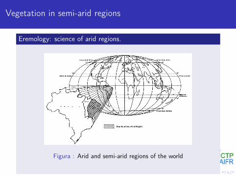
Vegetation in semi-arid regions

Eremology: science of arid regions.

Figura : Arid and semi-arid regions of the world

Vegetation in semi-arid regions

Eremology: science of arid regions.

Figura : Arid and semi-arid regions of the world

Vegetation in Semi-Arid Regions

Figura : Bahia

Consider the vegetation cover inwater-poor regions.

In this case, water is a limiting factor.quite different from tropical regions,where competition for water is irrelevant.One of the main limiting factor is light.

We want to build a mathematical model— (simple, please ) — to describe themutual relation between water in soil andbiomass in semi-arid regions.

Let us do it

Klausmeier Model

Figura : Colorado, USA

Figura : Kalahari, Namibia

Water and vegetation, in a firstapproximation, entertain a relation similar topredador-prey dynamics.

The presence of water is incremental forvegetation;

Vegetation consumes water.

But note that water does not originate fromwater.. It is an abiotic variable.

The usual predator-prey dynamics does notapply.

Consider two variables:w ,the amount of water in soil.u, the vegetation biomass (proportional to the area withvegetation cover).

Klausmeier Model

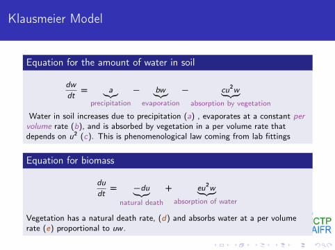
Equation for the amount of water in soil

dw

dt= a︸︷︷︸

precipitation

− bw︸︷︷︸evaporation

− cu2w︸ ︷︷ ︸absorption by vegetation

Water in soil increases due to precipitation (a) , evaporates at a constant pervolume rate (b), and is absorbed by vegetation in a per volume rate thatdepends on u2 (c). This is phenomenological law coming from lab fittings

Equation for biomass

du

dt= −du︸︷︷︸

natural death

+ eu2w︸ ︷︷ ︸absorption of water

Vegetation has a natural death rate, (d) and absorbs water at a per volumerate (e) proportional to uw .

Analysis

dwdt = a− bw − cu2w du

dt = −du + eu2w

Let us begin by defining two new variables, rescaled ones:

W = w

[e√b3c

]U = u

√bc

T = tb

They are dimensionless.Plug them into the equations and you will get....

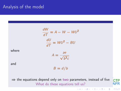
Analysis of the model

dW

dT= A−W −WU2

dU

dT= WU2 − BU

whereA =

ae√b3c

andB = d/b

⇒ the equations depend only on two parameters, instead of fiveWhat do these equations tell us?

Analysis of the model

dWdT

= A−W −WU2 dUdT

= WU2 − BU

Let us look for fixed points:

The points U∗ e W ∗ such that

dW ∗

dT= 0

dU∗

dT= 0

or

A−W ∗ −W ∗(U∗)2 = 0

W ∗(U∗)2 − BU∗ = 0

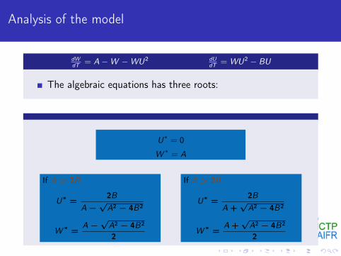
Analysis of the model

dWdT

= A−W −WU2 dUdT

= WU2 − BU

The algebraic equations has three roots:

U∗ = 0

W ∗ = A

If A > 2B

U∗ =2B

A−√A2 − 4B2

W ∗ =A−√A2 − 4B2

2

If A > 2B

U∗ =2B

A +√A2 − 4B2

W ∗ =A +√A2 − 4B2

2

Analysis of the Model

Interpretation

Our first conclusion:

If A < 2B the only solution is U∗ = 0 e W ∗ = A.This represents a bare state. A desert.

The condition A > 2B ⇒ a > 2d√

bce

shows that there mustbe a minimum amount of precipitation to sustain vegetation.Moreover, the higher e the easier to have a state withvegetation.Recall that e represents the absorption rate. Thehigher, the better.On the other, the higher (b) and the death rate of thepopulation, (d) easier it is to have a vegetationless solution.Seems reasonable!

Analysis of the model

So, let A > 2B

If A > 2B, we can have two fixed points.

What about their stability?.

The linear stability analysis results in:The fixed point U∗ = 0 and W ∗ = A is always stable.The fixed point

U∗ =2B

A+√A2 − 4B2

, W ∗ =A+√A2 − 4B2

2

is always unstable.The fixed point

U∗ =2B

A−√A2 − 4B2

,W ∗ =A−√A2 − 4B2

2

is always stable.

Analysis of the Model

So, if A > 2B, and B > 2, we have two stable fixed points, each of themwith its basin of attraction.

A pictorial view is as follows:

Figura : B is fixed, and we plot U∗ ( the biomass ) in terms of A. Thesolution representing a desert (U∗ = 0) and the solution corresponding tovegetation cover are both stable

Hysteresis

The existence of a region of bi-stability (A > 2B, B > 2), can take us tothe following situation.

Take a fixed B. Consider that A can change slowly ( think of a moreformal definition of "slowly").

Let us begin in the bi-stability. And let A decrease. At a certain moment,A will cross the critical value A = 2B.

At this time a sudden transition occurs, a jump, in which U∗ → 0.Desertification!!!.Suppose now that A begins again to increase - slowly. As U∗ = 0 isstable, even with A > 2B we will continue in the "desertic"region, as atthe moment of crossing back the critical point we were in its the basin ofattraction..

In summary: if we begin with a certain A, decrease it A < 2B and thencome back to our initial value of A, the state of the system can transitfrom U∗ 6= 0 to U∗ = 0.This is called Hysteresis.

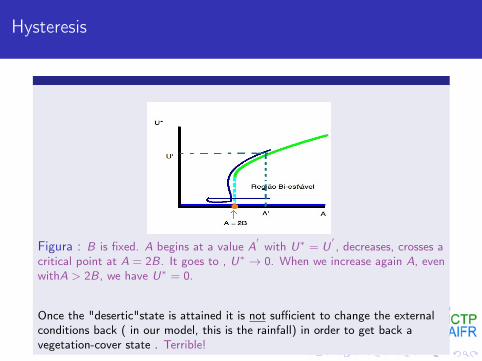
Hysteresis

Figura : B is fixed. A begins at a value A′with U∗ = U

′, decreases, crosses a

critical point at A = 2B. It goes to , U∗ → 0. When we increase again A, evenwithA > 2B, we have U∗ = 0.

Once the "desertic"state is attained it is not sufficient to change the externalconditions back ( in our model, this is the rainfall) in order to get back avegetation-cover state . Terrible!

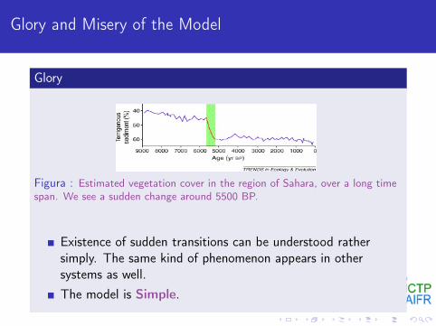
Glory and Misery of the Model

Glory

Figura : Estimated vegetation cover in the region of Sahara, over a long timespan. We see a sudden change around 5500 BP.

Existence of sudden transitions can be understood rathersimply. The same kind of phenomenon appears in othersystems as well.The model is Simple.

Glory and Misery of the Model

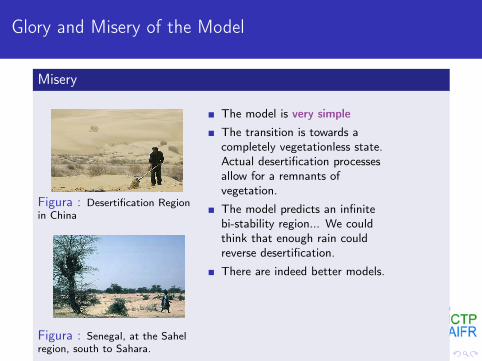
Misery

Figura : Desertification Regionin China

Figura : Senegal, at the Sahelregion, south to Sahara.

The model is very simpleThe transition is towards acompletely vegetationless state.Actual desertification processesallow for a remnants ofvegetation.

The model predicts an infinitebi-stability region... We couldthink that enough rain couldreverse desertification.

There are indeed better models.

More realistic models

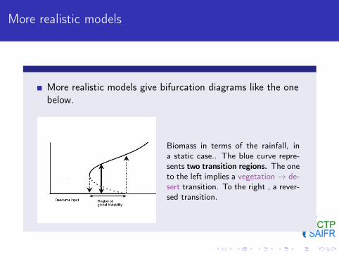
More realistic models give bifurcation diagrams like the onebelow.

Biomass in terms of the rainfall, ina static case.. The blue curve repre-sents two transition regions. The oneto the left implies a vegetation→ de-sert transition. To the right , a rever-sed transition.

More realist models

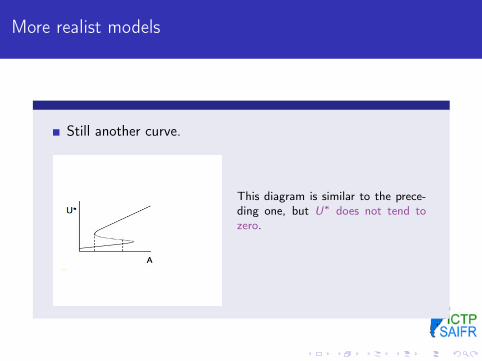
Still another curve.

This diagram is similar to the prece-ding one, but U∗ does not tend tozero.

Bibliography

M. Scheffer e S.R. Carpenter, Trends in Ecology and Evolution18, 648 (2003).M. Rietkerk et alli., Science 305, 1926 (2004)C.A. Klausmaier, Science 284, 1826 (1999).M. Scheffer, Critical Transitions in Nature and Society(Princeton U. P. 2009).