ii - ETD - Electronic Theses &...

REDUCING UNCERTAINTY IN THE CHARACTERIZATION AND MODELING OF

REACTIVE TRANSPORT PROCESSES IN BLENDED CEMENT MORTAR

By

Joshua R. Arnold

Dissertation

Submitted to the Faculty of the

Graduate School of Vanderbilt University

in partial fulfillment of the requirements

for the degree of

DOCTOR OF PHILOSOPHY

in

Environmental Engineering

May, 2014

Nashville, Tennessee

Approved:

Professor David S. Kosson

Professor Andrew C. Garrabrants

Professor John Ayers

Dr. Christine Langton

Professor J.C.L. Meeussen

Professor Florence Sanchez

Dr. Hans van der Sloot

ii

Copyright © 2014 by Joshua R. Arnold

All Rights Reserved

iii

DEDICATION

To my mother and father, without whom I should have long since perished

To my brother for continually challenging my ways of thinking, and

To my grandmother for the enthusiastic encouragement of my lifelong education.

To all my family and friends for lifting my spirits and

To the people of earth, who may hopefully benefit from this work.

iv

ACKNOWLEDGMENT

This work was prepared with the financial support by the U. S. Department of Energy, under

Cooperative Agreement Number DE-FC01-06EW07053 entitled 'The Consortium for Risk

Evaluation with Stakeholder Participation III' awarded to Vanderbilt University. This research

was carried out as part of the Cementitious Barriers Partnership supported by U.S. DOE Office

of Environmental Management. The opinions, findings, conclusions, or recommendations

expressed herein are those of the authors and do not necessarily represent the views of the

Department of Energy or Vanderbilt University.

v

TABLE OF CONTENTS

Page

ACKNOWLEDGMENT................................................................................................................ iv

LIST OF TABLES .......................................................................................................................... x

LIST OF FIGURES ...................................................................................................................... xii

LIST OF ABBREVIATIONS AND SYMBOLS ......................................................................... xx

Chapter

1. INTRODUCTION ................................................................................................................. 1

1.1. Motivation ........................................................................................................................ 1

1.2. Research Goal and Specific Objectives ........................................................................... 3

2. IONIC TRANSPORT IN CEMENT-BASED MATERIALS ............................................... 6

Abstract ....................................................................................................................................... 6

2.1. Introduction ...................................................................................................................... 6

2.2. Models and methods......................................................................................................... 9

2.2.1. Simulation geometry ................................................................................................. 9

2.2.2. Reactive transport model formulation ...................................................................... 9

2.2.3. Geochemical reaction.............................................................................................. 12

2.2.4. Solution strategy ..................................................................................................... 14

2.2.5. Numerical method ................................................................................................... 14

2.3. Model parameterization.................................................................................................. 17

2.3.1. Initial and boundary conditions .............................................................................. 17

2.3.2. Thermodynamic constants ...................................................................................... 19

vi

2.3.3. Activity coefficients ................................................................................................ 23

2.3.4. Ionic diffusion coefficient estimation ..................................................................... 24

2.4. Results and discussion .................................................................................................... 27

2.4.1. Example 1: Comparison of Fickian and LEN transport in an inert porous medium ..

................................................................................................................................. 27

2.4.2. Example 2: Dilute external leachant ....................................................................... 29

2.4.3. Example 3: Concentrated single-salt leachant ........................................................ 33

2.4.4. Example 4: Concentrated multi-ionic leachant ....................................................... 39

2.5. Conclusions .................................................................................................................... 44

3. SOLUTION OF THE NONLINEAR POISSON-BOLTZMANN EQUATION:

APPLICATION TO CEMENTITIOUS MATERIALS................................................................ 46

Abstract ..................................................................................................................................... 46

3.1. Introduction .................................................................................................................... 46

3.2. Experimental Methods ................................................................................................... 50

3.2.1. Sample preparation ................................................................................................. 50

3.2.2. Pore water expression ............................................................................................. 50

3.2.3. Porosimetry ............................................................................................................. 51

3.3. EDL modeling ................................................................................................................ 51

3.4. Results and Discussion ................................................................................................... 55

3.4.1. Porewater concentrations ........................................................................................ 55

3.4.2. Porosimetry ............................................................................................................. 55

3.4.3. EDL Modeling ........................................................................................................ 57

3.4.3.1. Academic examples ......................................................................................... 58

3.4.3.2. Application to blended cement mortar ............................................................ 60

3.4.3.3. Interpretation of diffusion cell experiments .................................................... 62

vii

3.5. Conclusions .................................................................................................................... 68

4. BACKSCATTERED ELECTRON MICROSCOPY AND ENERGY DISPERSIVE X-

RAY ANALYSIS FOR QUANTIFICATION OF THE REACTED FRACTIONS OF

ANHYDROUS PARTICLES IN A BLENDED CEMENT MORTAR ....................................... 69

Abstract ..................................................................................................................................... 69

4.1. Introduction .................................................................................................................... 69

4.2. Materials and experimental methods.............................................................................. 71

4.2.1. Sample preparation ................................................................................................. 72

4.2.2. Scanning and processing ......................................................................................... 73

4.2.3. Sources of experimental uncertainty ....................................................................... 74

4.3. Particle identification method ........................................................................................ 77

4.3.1. Segmentation........................................................................................................... 78

4.3.2. Anhydrous particle database – cluster analysis ...................................................... 85

4.3.3. Particle classification - discriminant analysis ......................................................... 86

4.3.4. Calculation of reacted fraction ................................................................................ 87

4.4. Results and Discussion ................................................................................................... 88

4.4.1. Anhydrous particle database ................................................................................... 88

4.4.2. Database cross-validation ....................................................................................... 92

4.4.3. Estimation of reacted fractions ............................................................................... 96

4.5. Conclusions .................................................................................................................... 99

5. CHARACTERIZATION AND MODELING OF MAJOR CONSTITUENT

EQUILIBRIUM CHEMISTRY OF A BLENDED CEMENT MORTAR ................................. 101

Abstract ................................................................................................................................... 101

5.1. Introduction .................................................................................................................. 101

5.2. Methods ........................................................................................................................ 102

viii

5.2.1. Material preparation .............................................................................................. 102

5.2.2. pH-dependent leaching test ................................................................................... 103

5.2.3. Geochemical modeling ......................................................................................... 104

5.3. Results and discussion .................................................................................................. 106

5.4. Conclusions .................................................................................................................. 113

6. REACTIVE TRANSPORT MODELING OF EXTERNALLY-INDUCED AGING OF

BLENDED CEMENTITIOUS MATERIALS ........................................................................... 115

Abstract ................................................................................................................................... 115

6.1. Introduction .................................................................................................................. 115

6.2. Materials and methods ................................................................................................. 117

6.2.1. Component materials ............................................................................................ 117

6.2.2. pH dependent leaching .......................................................................................... 118

6.2.3. Accelerated aging.................................................................................................. 119

6.3. Reactive transport modeling......................................................................................... 120

6.3.1. Geochemical equilibrium modeling ...................................................................... 120

6.3.2. Mass transport modeling ....................................................................................... 122

6.4. Results .......................................................................................................................... 123

6.4.1. Reacted fractions and availabilities ...................................................................... 123

6.4.2. Geochemical equilibrium modeling ...................................................................... 125

6.4.3. Tortuosity determination ....................................................................................... 130

6.4.4. SVC leaching ........................................................................................................ 135

6.5. Conclusions .................................................................................................................. 139

7. CONCLUSIONS AND FUTURE WORK ........................................................................ 141

APPENDIX A: THERMODYNAMIC CONSTANTS FOR AQUEOUS SPECIES ................. 145

ix

APPENDIX B: THERMODYNAMIC CONSTANTS FOR SOLID SPECIES ........................ 146

APPENDIX C: ESTIMATED DIFFUSION COEFFICIENTS .................................................. 147

APPENDIX D: ANHYDROUS PARTICLE DATABASE OF ELEMENTAL COMPOSITIONS

..................................................................................................................................................... 149

REFERENCES ........................................................................................................................... 150

x

LIST OF TABLES

Table Page

2.1. Masses of primary species used as input to ORCHESTRA for an 85% hydrated Portland

cement paste. ........................................................................................................................ 18

2.2. Masses of the primary species of the three external solutions considered: deionized water

(DI), ammonium nitrate (AN), and 3× diluted waste form porewater (WF) ....................... 19

2.3. Calculated equilibrium concentrations of primary species in the native Portland cement

pore solution......................................................................................................................... 20

2.4. Ionic species used for estimation of unknown ionic diffusion coefficients ......................... 25

3.1. Apparent diffusivities reported in the literature from diffusion cell experiments on

cementitious materials ......................................................................................................... 48

3.2. Proportion of mix components............................................................................................. 50

3.3. Expressed pore water concentrations ................................................................................... 55

3.4. Results of ASTM C 642 density and water accessible porosity determination, mercury

intrusion porosimetry, and N2 adsorption ............................................................................ 56

3.5. Statistics computed from the beta distribution fit to the N2 adsorption incremental volume

curve ..................................................................................................................................... 57

4.1. Major element composition of the component materials ..................................................... 71

4.2. Mix design of the blended cement mortar ........................................................................... 72

5.1. Raw material properties of the mortar ............................................................................... 103

5.2. Major element composition of the binder materials .......................................................... 103

5.3. Solid phases considered in the SVC assemblage ............................................................... 105

6.1. Major element composition of the component materials ................................................... 117

6.2. Mix design of the blended cement mortar. ........................................................................ 118

6.3. Equivalent base additions and resultant pH for the Method 1313 leach test ..................... 119

xi

6.4. Solid species considered in equilbrium model of blended cement mortar ........................ 122

6.5. Masses of the primary species used as input for equilibrium modeling. ........................... 124

xii

LIST OF FIGURES

Figure Page

2.1. Modeled pH dependent solubility of primary species in typically cationic and typically

anionic form in hydrated Portland cements ......................................................................... 22

2.2. Fitted linear regressions of ionic diffusion coefficient values ............................................. 26

2.3. Comparisons of concentration depth profiles at 7 days of simulation time for DI water

leaching. ............................................................................................................................... 28

2.4. Comparison of pH, Ca, Al, and Si aqueous concentration profiles predicted by the Fickian

and LEN transport models for the case of DI water leaching of PC after 280 days of

simulated leaching ............................................................................................................... 30

2.5. Comparison of typically cationic primary species profiles predicted by the Fick and LEN

transport models for the case of DI water leaching of PC. .................................................. 31

2.6. Comparison of typically anionic primary species profiles predicted by the Fick and LEN

transport models for the case of DI water leaching of PC. .................................................. 32

2.7. Mass of hydrated PC phases after 280 days of simulated DI water leaching ...................... 33

2.8. Comparison of pH, Ca, Al, and Si aqueous concentration profiles predicted by the Fickian

and LEN transport models for the case of AN leaching of PC after 280 days of simulated

leaching ................................................................................................................................ 34

2.9. Comparison of ammonium and nitrate primary species concentration profiles predicted by

the Fick and LEN transport models for the case of AN leaching of PC .............................. 35

2.10. Distribution of predominant NH4 species and NO3 species within the pore solution after 28

days of simulated AN leaching using the LEN model ......................................................... 36


transport models for the case of AN leaching of PC. .......................................................... 37


transport models for the case of AN leaching of PC. .......................................................... 38

xiii

2.13. Profile of the predicted mass of hydrated PC phases after 280 days of AN leaching ......... 39

2.14. Comparison of concentration profiles of pH, Ca, Si, and Al predicted by the Fickian and

LEN transport models for the case of WF leaching of PC .................................................. 40


transport models for the case of WF leaching of PC ........................................................... 41

2.16. Comparison of the Mg-bearing solid phases predicted by the a) Fickian and b) LEN

reactive transport models ..................................................................................................... 42

2.17. Profile of the predicted mass of hydrated PC phases after 280 days of WF leaching ......... 43


transport models for the case of WF leaching of PC ........................................................... 44

3.1. Cumulative intrusion volume and differential intrusion volume for MIP intrusion cycles

and for N2 adsorption and desorption ................................................................................. 56

3.2. Experimentally determined N2 adsorption incremental volume curve and a beta distribution

fit to the curve ...................................................................................................................... 57

3.3. Simulated potential profiles for a 10 nm wide pore with constant surface potential of -25

mV for four acadmic pore solutions .................................................................................... 59

3.4. Normalized ion concentrations for variable pore diameters as a function of pore solution

ionic strength ........................................................................................................................ 61

3.5. Depiction of the 3-d bottle-necking pore and a schematic indicating the more tortuous

cation path and the local distribution of anions when considering ink-bottle pores ............ 66

3.6. Electrostatic potential contour plots and concentration profiles for two cylindrical pores

connected by a bottle-neck pore .......................................................................................... 67

4.1. Probability density function representation of particle size (diameter) distributions for BFS,

FAF, and OPC particles ....................................................................................................... 76

4.2. Data flow diagram of particle identification algorithm implemented in this work ............. 78

4.3. An example of the DDLP algorithm applied to a fly ash BSE image ................................. 81

xiv

4.4. Diagram of mass fractions of BFS composition measured via XRF and the centroid

composition as calculated by the MBC method .................................................................. 89

4.5. Diagram of the mass fractions of the bulk FAF composition (FAF), and the FAF subtypes

(FAFa,b,c) identified using the MBC method ........................................................................ 89

4.6. BSE micrograph of QS quartz sand aggregate with lath-shaped phyllosilicates ................. 90

4.7. Measured distributions of particle eccentricities of the kaolinite and illite particles

measured in the QS material ................................................................................................ 91

4.8. Diagram of the mass fractions of the anhydrous particle database used for particle

classification ........................................................................................................................ 91

4.9. Results of the LDA classification algorithm applied to BFS particles mounted in resin .... 93

4.10. Area dependence of the LDA particle classification algorithm illustrated for BFS particles

mounted in methacrylate resin ............................................................................................. 94

4.11. Results of the LDA classification algorithm applied to FAF particles mounted in resin .... 95

4.12. Results of the LDA algorithm applied to SVC mortar ........................................................ 96

4.13. Results of the LDA algorithm applied to SVC mortar with phyllosilicates in the field of

view ...................................................................................................................................... 98

4.14. Results of the LDA algorithm applied to SVC mortar using geometric descriptors of

phyllosilicates ...................................................................................................................... 99

5.1. Comparison of modeled and measured major constituent leachate concentrations of

USEPA Method 1313 performed on SVC ......................................................................... 108

5.2. Comparison of modeled and measured major constituent leachate concentration. ........... 109

5.3. BSE micrograph of kaolinite formation in close proximity to a fly ash particle in the SVC

material .............................................................................................................................. 110

5.4. Backscattered electron micrographs of a phyllosilicate presumed to be kaolinite and illite

............................................................................................................................................ 111

5.5. Modeled and experimental equilibrium concentrations of total dissolved Al ................... 111

xv

5.6. Backscattered electron micrograph of a partially hydrated slag particle in unaltered SVC

............................................................................................................................................ 113

6.1. Graphical representation of the molar proportions of major primary species participating in

the partial equilibrium assemblage as predicted by the availability from Method 1313 and

from the sum of reacted fractions ...................................................................................... 124

6.2. The response of system pH in both simulation and experiment as a function of

milliequivalents of base added per gram of solid material ................................................ 126

6.3. Contour plots of the mean errors in major primary species computed from comparison of

model responses to pH-dependent batch leaching ............................................................. 127

6.4. Contour plots of the mean errors in alkali primary species computed from comparison of

model responses to pH-dependent batch leaching ............................................................. 128

6.5. Experimentally measured values of component solubility from the Method 1313 leaching

protocol and geochemical equilibrium modeling results using both availabilities and

reacted fractions ................................................................................................................. 129

6.6. Mean squared errors computed from comparison of simulation and experimental data for

the DI leaching case ........................................................................................................... 131

6.7. Comparison of modeled and experimentally measured tank concentrations of alkali ions in

the DI water leaching scenario using values of 𝜏 = 500 and 𝜏 = 60,000 ........................ 133

6.8. Comparison of modeled and experimentally measured tank concentrations of major ions in

the DI water leaching scenario using values of 𝜏 = 500 and 𝜏 = 60,000 ........................ 134

6.9. Comparison of modeled and experimentally measured tank pH in the DI water leaching

scenario using values of 𝜏 = 500 and 𝜏 = 60,000 ........................................................... 135

6.10. Experimentally measured tank concentrations of Na and K as a function of the square root

of leaching time for the four leaching cases ...................................................................... 136

6.11. Experimentally measured and simulated tank concentrations of Si as a function of the

square root of leaching time for DI, NC, MS, and NS leaching ........................................ 137

xvi

6.12. Experimentally measured and simulated tank concentrations of Al as a function of the


6.13. Experimentally measured and simulated tank concentrations of Mg as a function of the


6.14. Experimentally measured and simulated tank concentrations of Ca as a function of the


6.15. Experimentally measured and simulated values of tank pH as a function of the square root

of leaching time for DI, NC, MS, and NS leaching ........................................................... 139

xvii

LIST OF ABBREVIATIONS AND SYMBOLS

List of abbreviations

AN ammonium nitrate solution

BFS blast furnace slage

BSEM backscatter scanning electron microscopy

C-S-H calcium silicate hydrate

DDLP Delon, Desolneux, Lisani, and Petro segmentation algorithm

DI deionized water solution

EDX enery dispersive X-ray analysis

FAF class F fly ash

FD finite difference

LDA linear discriminant analysis

LEN local electroneutral

LHS Latin hypercube sampling

keV kilo-electron volts M moles per liter

M-S-H magnesium silicate hydrate

MIP mercury intrusion porosimetry

MS magnesium sulfate, MgSO4

NC sodium carbonate, Na2CO3

NP Nerst-Planck

NS sodium sulfate, Na2SO4

OPC ordinary Portland cement

PBE Poisson-Boltzmann equation

PC Portland cement

PDE partial differential equation

PVA partial volume averaging

QS quartz sand

SCM supplementary cementitious material

SVC structural vault concrete analogue

xviii

List of abbreviations, continued

USEPA United States Environmental Protection Agency

w/b water-to-binder ratio

WF waste form solution

XRF X-ray fluourescence

List of English symbols

𝐶𝑖 concentration of species 𝑖 in solution

𝑑𝐾𝑂 depth of electron interaction volume

𝐷𝑖 phenomenolical diffusion coefficient

𝐷𝑖𝑜𝑏𝑠 observed diffusion coefficient

𝐷𝑖𝑢 ionic diffusion coefficient

𝑒 elementary electron charge

𝐸0 SEM excitation energy

F Faraday’s constant

𝐹𝑖 rate of reaction of species 𝑖

𝐽𝑖 flux of species 𝑖

kB Boltzmann’s constant

𝐾𝑖, 𝐾ℓ thermodynamic stability constant of species 𝑖, ℓ

𝑀𝑝 moles of primary species 𝑝

NA Avogadro’s number

R ideal gas constant

𝑅 retardation factor

𝑆𝑖 sorbed concentration of species 𝑖

𝑇 temperature

𝑍𝑎𝑣𝑒 average charge

𝑧𝑖 formal charge of species 𝑖

xix

List of Greek symbols

𝛼𝑞 reacted fraction of component 𝑞

𝛾𝑖 activity coefficient of species 𝑖

ϵ dielectric constant

ϵ0 permittivity of free space

ϵr relative perimittivity coefficient

𝜇𝑖 chemical potential of species 𝑖

𝜌 density

𝜏 tortuosity

𝜈𝑝𝑖, 𝜈𝑝ℓ stoichiometric coefficient of species 𝑝 in species 𝑖, ℓ

𝜙 porosity

𝜓 electric potential

1

CHAPTER 1

1. INTRODUCTION

1.1. Motivation

For two millennia, anecdotal knowledge has sustained the practice of cement-based construction,

the success of which is evidenced by the perseverance of several iconic structures of the Roman

Empire. In modern times, the requirements of cementitious structures are constantly evolving;

the burgeoning demand for infrastructure in the developing world and the concomitant need to

minimize environmental and economic costs can very likely only be met with the use of concrete

construction. Already in the last half century, the incorporation of byproducts and “waste”

materials, such as blast furnace slag, coal combustion fly ash, municipal waste ash, and a myriad

of others, has become a prevalent strategy for reducing the economic and carbon costs of

Portland cement production while, in some cases, simultaneously improving the physical and

chemical properties of the composite cement system. Moreover, the technological advances of

the last quarter-century, particularly the advent of nano-engineered materials, have spurred the

quest for newer, “smarter” cementitious composites designed to suit a plethora of needs. The

common thread among these novel materials, sundry as they may be, is that they push the

envelope of mechanistic understanding well beyond the scope of anecdotal knowledge at a pace

that empiricism struggles to maintain. It is within this envelope that the “virtual laboratory” lies;

modeling allows the interplay of physico-chemical behaviors to be examined within regimes that

are impractical or impossible to access through actual experimentation. The onus on the scientist

and engineer, then, is to model these systems in ways which are sensitive to the variations likely

to occur throughout the lifetime of the system, and this may be accomplished, perhaps most

effectively, through investigation of the fundamental mechanisms that govern physico-chemical

behaviors. Such an approach avails itself to the problem of uncertainty analysis especially, in that

the influence of individual component mechanisms on the holistic system response may be

ascertained, whereas purely empirical models may only be varied in terms of parameters that

may possess little to no physical significance. Furthermore, as the understanding of fundamental

mechanisms improves, this new information may be assimilated into mechanistic models with

2

relative ease, allowing the examination of new interconnected behaviors, and it is through the

elucidation of these interconnections that the virtual laboratory proves its worth.

A prime example of mechanistic-based modeling of inaccessible regimes is the prediction of the

long-term performance of cementitious barriers used in nuclear waste management applications.

Such predictions assess the behavior of the engineered system with respect to both contaminant

retention and structural integrity, which entails mechanistic modeling of the system’s physico-

chemical behavior and quantifying the uncertainty about those model predictions. The

Cementitious Barriers Partnership (CBP, http://cementbarriers.org/) is charged with the task of

developing software tools that aim to reduce uncertainties in the performance assessment of

cementitious barriers. The CBP has made considerable progress towards its goal on three general

fronts: characterization, modeling, and uncertainty quantification. A significant amount of

experimental characterization has been performed by the CBP, both in defining reference

cementitious materials for study, which are representative of those used in practice [1], and in the

rigorous measurement of their chemical and physical properties [2-4]. Considerable progress has

also been made in both demonstrating state-of-the-art modeling capabilities [5-8], improving

phenomenological models [9, 10], and in quantifying the uncertainties inherent in both models

and measurements [11, 12]. It is within the CBP framework that this dissertation thesis resides.

The aim of this work is to elucidate the origins and relative magnitudes of uncertainties within

the reactive transport modeling of externally-induced aging processes in cementitious systems.

An “externally-induced aging process” is herein defined as a perturbation of the physico-

chemical cement-based system due to its disequilibrium with the ambient environment. Thus,

autogeneous aging processes are neglected, but even so, the scope of this definition is vast.

Therefore, externally-induced aging processes are further restricted to those due to aqueous

phase diffusive transport between the cementitious porewater and an external reservoir, namely

“leaching”. The cementitious material studied in this work is a CBP reference material, a blended

cement mortar supplemented with ground granulated iron blast furnace slag and coal combustion

fly ash. These two supplementary cementitious materials have found widespread utility

commercially as well as in nuclear waste management applications.

This work identifies critical parametric and model uncertainties within three core aspects of

mechanistic reactive transport modeling for blended cementitious materials: mass transport, mass

3

conservation, and thermodynamic characterization. Mass transport encompasses the modeling of

ionic motion due to diffusive processes, that is, the interaction of aqueous species, as well as the

interaction of aqueous species with charged surfaces. Mass conservation entails the

parameterization of total elemental mass which is considered to be reactive within the

cementitious matrix, and thermodynamic characterization concerns the partitioning of that mass

into various solid and aqueous species. Comparing and contrasting both modeling methods and

experimental techniques in these core areas facilitate the identification of the origins of

uncertainties.

1.2. Research Goal and Specific Objectives

The goal of the research presented here is the identification of uncertainties in the experimental

characterization and simulation of aging processes in a blended cement mortar. The specific

objectives are:

1. To assess the differences in predicted rate of release from cementitious materials as a

result of either assuming a Fickian or Nernst-Planck-Poisson model of solute transport.

2. To model the electric double layer on idealized cementitious pore walls for measured

blended cement porewater compositions and to assess the potential impacts of the electric

double layer on the rate of transport through the cement pore space.

3. To develop a method of quantifying the extent of anhydrous particle reaction in blended

cement mortars for the purpose of informing geochemical reactive transport modeling of

cement.

4. To model the equilibrium chemistry of a blended cement mortar using thermodynamic

parameters developed for the description of ordinary Portland cement systems and to

assess the ability of this set of parameters to describe the blended cement chemistry by

comparison to experimental data.

5. To employ reactive transport modeling to describe the transient chemical behaviors of a

blended cement mortar monolith as the result of exposure to various external aging

solutions and to evaluate the applicability of Portland cement thermodynamic parameters

for describing this system.

4

In Chapter 2, the transport process itself is scrutinized, as the Fickian diffusion model is

compared to the Nernst-Planck (NP) charge-coupling migration model within the context of

reactive transport in a fictitious Portland cement. The application of the NP model to a reactive

system with homogeneous aqueous phase reactions is, to the author’s knowledge, the first of its

kind for cementitious materials. In Chapter 3, the Poisson-Boltzmann equation (PBE), which

describes the electrostatics of the electric double layer in the vicinity of charged surfaces, is

solved for a real blended cement porewater composition without “usual and customary”

assumptions that are typically not applicable to cement-based systems. With the PBE solution for

hypothetical pores and experimental measurements of pore size distributions of a blended cement

mortar, inductive arguments are made for considering the electric double layer as a potentially

significant factor in determining the transient movement of ions within cementitious porewaters.

Chapter 4 departs from the diffusive process in order to demonstrate a novel method of

characterizing and quantifying the extent of reaction of highly heterogeneous blended cement

systems, supplemented with iron blast furnace slag and coal combustion residue, using

probabilistic techniques applied to backscattered scanning electron microscopic and energy

dispersive X-ray spectroscopic information. Extent of reaction is a key parameter for

determining the chemical properties of systems containing supplementary cementitious

materials, and the reliable quantification of the degree of reaction in supplementary cementitious

materials has been identified as a major need within the field [13]. In Chapter 5, the extent of

reaction is used to determine the masses of the “partial equilibrium assemblage”, that is, the mass

of major constituents within the reacted portion of a blended cement system. A set of solid phase

equilibrium constants developed for describing Portland cement systems is used in conjunction

with the reacted to mass to compute the pH-dependent solubility of the same blended cement

system. Given that the reaction product of ashes and slags in cement systems are largely

unknown, the comparison of these simulations to batch leaching experiments serve as a guide for

assessing the limitations of current thermodynamic data for describing these complex systems.

Chapter 6 is the culmination of the results of the previous four chapters in that the transient

leaching behavior of the blended cement is modeled and compared to experimentally measured

values of major constituent release. In this study, cement monoliths are exposed to external aging

solutions which are intended to elicit the mineralogical changes expected in natural

5

environments. The ability of the Portland cement solid phases to characterize the monolith

leaching behavior is evaluated and the potential limitations of the current thermodynamic

understanding of these systems are highlighted.

6

CHAPTER 2

2. IONIC TRANSPORT IN CEMENT-BASED MATERIALS

Abstract

The local electroneutral form of the Nernst-Planck (NP) equations, derived from the null-current

assumption, is employed to model the transport of multiple ionic species in aqueous solution.

Predictions of primary ion solubility profiles are compared to those of the more common Fickian

diffusion model within the context of a practical problem, leaching of a hydrated Portland

cement paste. Differences between Fickian and NP transport are highlighted for three distinct

external solution leaching scenarios: deionized water, ammonium nitrate solution, and a diluted

porewater from a cementitious low-activity nuclear waste form. Although small differences are

observed in the case of deionized water leaching, differences of as much as a factor of four are

observed in the concentration profiles of certain species in the ammonium nitrate and simulated

waste form solution leaching cases. Thus, the choice of transport model may influence

predictions of contaminant release and degradation rates.

2.1. Introduction

Understanding the fundamental mechanisms of ion transport is key to assessing the long-term

performance of cementitious materials. Whether predicting the rate of decalcification, of ingress

of chloride, or of release of radionuclides from a cementitious waste matrix, there exists an

unequivocal need for describing solute transport. Traditionally, transport phenomena in porous

cementitious media have been described using the Fickian diffusion model; however, more

complex electro-diffusion models have been proposed recently with the goal of improving

predictive capability. One of complexities of ionic transport in porous cements arises from the

presence of numerous (≈ 50) ionic species in the pore solution. In this article, we investigate the

differences in ionic concentrations predicted by two distinct transport models, namely Fickian

diffusion and electro-diffusion, and address a fundamental question: what is the importance of

7

the Coulombic interactions between the numerous ions in the cement pore solution as well as

those present in the external environment?

The first model to describe solute transport in the absence of advection be attributed to Adolf

Fick who, in 1855 [14], first put forth the observation that a solute diffuses proportionally to its

concentration gradient. Existing studies on leaching commonly employ the Fickian diffusion

model to describe the transport of only a few ionic species thereby neglecting the physical

constraint that the solution remain electroneutral. Another common practice is to employ single

diffusion coefficient for all species in solution, which, when starting from an electroneutral

initial condition, serves to maintain local electroneutrality [11, 15, 16]. Experimentally obtaining

ion-specific Fickian diffusion coefficients may be both tedious and challenging because of their

dependence upon the system state, as evidenced by the large number of empirical concentration-

dependent diffusion coefficients found in the literature [17-21]. In contrast, the Nernst-Planck

(NP) transport model provides a mechanism for maintaining electroneutrality (in the absence of

applied potential), and may account for some concentration-dependent diffusive behavior given

an appropriate chemical activity model. In 1888, Walther Nernst asserted that the transport of an

ion is proportional to its electrochemical potential gradient. The NP model has been adopted and

amended by a number of disciplines, most notably for describing ionic transport in proteins [22-

25], in highly concentrated and ionic liquids [26-29], in nanofluidic channels [30-33], and in

clays [34-39].

For modeling transport in cementitious materials, the application of the NP model has gained

popularity in recent decades. Samson and co-workers [40, 41] employed the NP to the problem

of describing ionic migration under an applied electric current for the interpretation of

accelerated migration experiments, and a handful of studies have applied the NP to describe

ionic migration in cementitious materials for various purposes [41-46]. Snyder and Marchand

[47] carried out an experimental investigation of the case of zero external potential in

nonreactive porous frit exposed to various initial and boundary conditions; their findings

indicated that simple Fickian diffusion could not adequately describe multi-ionic diffusion and in

some cases the fitted value of the Fickian diffusion coefficient became negative, that is, a species

was transported against its concentration gradient. Samson and Marchand [48] also found close

agreement between their NP results and experimental measurement of sulfate ingress fronts but

8

did not compare their results to the Fickian case. Galíndez and Molinero [49] compared Fickian

and NP transport model results of sulfate attack of a cement paste using a limited number of

ionic species and found that the NP model predicted the presence of near-surface gypsum front,

whereas the Fickian model did not. These findings suggest that the Coulombic coupling of ions

manifest in the NP model may be a significant factor in determining net transport rates. What has

not been clearly established, however, is an explicit comparison of the Fickian and NP

formulations in the absence of an applied external field within the context of a reactive transport

simulation. Moreover, the long-term impacts of coupling of NP transport simulation with

homogeneous reactions in the aqueous phase have not been fully addressed for cementitious

systems [50]. Given that durability predictions depend upon transport predictions and that

lifetime performance assessment in turn depends upon durability predictions, a salient question is

whether the concentrations computed by the Fickian and NP models yield substantially different

results.

The purpose of this article is to directly compare the Fickian and NP mass transport models

within the context of a practical problem: aggressive leaching of a Portland cement. The three

aggressive leaching solutions considered herein, pertinent to testing and field performance

conditions, are deionized water, ammonium nitrate solution, and diluted porewater from a

simulated low-activity waste form; each of these leachants represents a distinctly different class

of solution: an infinitely dilute solution, a concentrated (≈ 1M) single-salt solution, and a

concentrated (≈ 1M) multi-ionic solution, respectively. The investigation of these three solutions

provides a basis for determining the conditions under which the differences between the Fickian

and NP models may be important.

The remainder of this article is organized as follows. In Section 2, the geometry and conceptual

model for simulation of the problem are outlined, and the governing equations and

approximations of the reactive transport model are given for both the Fickian and NP transport

model formulations. Due to its relative ease of implementation and computational efficiency, the

finite difference (FD) method of numerical approximation has been employed in this work to

simulate both Fickian and NP solute transport. In contrast to previous studies which employed an

explicit form of the FD method for solving the NP system of equations [34, 35] the present work

invokes the fully implicit FD method with Newton-Raphson iteration to account for the

9

nonlinear nature of the NP equations while allowing for arbitrarily large stable simulated time

step intervals. Section 3 presents the aqueous and solid phase thermodynamic parameters

necessary for calculating chemical equilibrium. The reactive transport of 81 aqueous species is

considered in this work, which requires 81 ionic diffusion coefficients for the NP model. These

diffusion coefficients remain unknown quantities for many of the aqueous species found to be

relevant in geologic media and commonly used in Portland cement modeling. In [49], six values

of ionic diffusion coefficient were provided for the approximately 30 aqueous species modeled,

creating some ambiguity as to the values prescribed for each ion. In this work, however, an

empirical relationship is proposed for correlating ionic diffusion coefficients for the ions in

question to both their formal charge and van der Waals volumes, which is discussed in Section

3.3. Section 4 compares the Fickian and NP ionic transport models for four example cases, first

within an inert porous medium and then within a reactive hydrated ordinary Portland cement

(PC), considering the aforementioned external solutions in contact with the cementitious

material. Section 5 recapitulates the major findings of each example case and summarizes the

practical significance of these findings within the context of cementitious material leaching.

2.2. Models and methods

2.2.1. Simulation geometry

All simulations are performed at standard temperature and pressure for the one-dimensional case

of a porous medium of length ℓ = 0.02 [m], porosity 𝜙 = 0.20 [m3 connected porosity per m3

total], and skeletal density of 2200 [kg/m3]. The simulation domain consists of 21 nodes equally

spaced at intervals of 1 mm. A single face of the medium, at 𝑥 = 0 is exposed to an external

solution of infinite volume such that the concentrations at the specimen-solution interface are

fixed (Dirichlet boundary). Concentrations are also fixed at the opposite face, at 𝑥 = ℓ, to the

initial porewater concentrations (Dirichlet boundary).

2.2.2. Reactive transport model formulation

In a saturated reactive porous medium, the mass conservation expression must reflect the

dissolution and precipitation reactions, that is,

10

∂𝐶𝑖𝜕𝑡

= −𝜕𝐽𝑖𝜕𝑥

− 𝐹𝑖 (2.1)

where 𝐶𝑖(𝑥, 𝑡) [mol/m3] refers to the concentration of 𝑖th species in the pore solution at spatial

location 𝑥 [m] and time 𝑡 [s], and 𝐽𝑖 [mol/m2/s] is the flux of species 𝑖. The reactive rate term 𝐹𝑖

[mol/m3/s] representing a phase change of 𝑖 from the aqueous phase to a solid precipitate phase.

Directly solving Eq. (2.1) is complex because the reactive term depends simultaneously on 𝐶𝑖

which requires an iterative scheme that can be computationally expensive [50]. In this work, the

sequential non-iterative algorithm (SNIA) has been employed [48, 51, 52], wherein the chemical

equilibrium and transport equations are solved in a staggered approach. In the first step, the

reaction terms are neglected in order to solve for concentration �̃�𝑖 which is not necessarily in

chemical equilibrium, as given by,

∂�̃�𝑖𝜕𝑡

= −𝜕𝐽𝑖𝜕𝑥

(2.2)

Throughout this chapter, �̃�𝑖 is referred to as the “uncorrected” concentration, because in the

second step of SNIA, the corrected concentration 𝐶𝑖 at the next time step is found from �̃�𝑖 by

solving for chemical equilibrium as described in Section 2.2.3.

Since Eq. (2.1) is derived from mass balance, it is generally valid with the flux 𝐽𝑖 given by either

the Fickian or NP transport model. As this chapter is concerned with the comparison of these two

models, it is necessary to clarify the mathematical differences between them, which is described

next.

Fickian diffusion model: For a nonreactive porous medium, the one-dimensional parabolic partial

differential equation describing the conservation of mass within an infinitesimally small control

volume may be written as [14, 53, 54]

𝐽𝑖 = −𝜏𝐷𝑖𝜕�̃�𝑖𝜕𝑥

(2.3)

where 𝜏 (≤ 1) is the tortuosity factor [m/m], which in the one-dimensional case is a scalar

quantity. The true physical significance of 𝜏 is not an entirely settled issue [55], but in this work,

𝜏 represents the physical resistance to diffusion resulting from increased diffusion path length

11

within a porous microstructure. The above Eq. (2.3) is generally valid for neutral (non-charged)

species, but not for ionic (charged) species if the system is to remain electrically neutral. When

considering the diffusion of only two oppositely charged species, that is 𝑖 = {1,2} and

sign(𝑧1) = −sign(𝑧2), the Coulombic coupling between charges requires that both species move

at an equivalent rate [56]:

𝐷1 = 𝐷2 =|𝑧1| + |𝑧2|

|𝑧1|/𝐷1𝑢 + |𝑧2|/𝐷2𝑢 (2.4)

where 𝑧𝑖 is charge and 𝐷𝑖𝑢 is herein termed the ionic diffusion coefficient at infinite dilution

[m2/s]. Thus, Eq. (2.3) is valid for describing diffusion in a dilute binary system provided that the

phenomenological diffusivity 𝐷𝑖 is the same for both ions. If more than two ionic species are

present in solution, 𝐷𝑖 can no longer be defined independently of the system state because

coupling of electrostatic forces occurs among all charged species, which necessitates the use of

the NP model described next.

Nernst-Planck (NP) model: The electrostatic coupling between multiple (i.e. more than two)

ionic species can be described by considering the electrochemical potential 𝜇𝑖 for each species

separately as,

𝜇𝑖 = 𝜇𝑖0 + R𝑇ln �𝛾𝑖�̃�𝑖� + 𝑧𝑖F𝜓 (2.5)

with 𝜇𝑖0 [J/mol] equal to the chemical potential at standard state, R [J/mol/K] the ideal gas

constant, 𝑇 [K] the absolute temperature, 𝛾𝑖 the activity coefficient, F [C/mol] Faraday’s

constant, and 𝜓 [V] the electric potential within the medium. Nernst hypothesized that the flux,

𝐽𝑖, is proportional to the gradient in 𝜇𝑖

𝐽𝑖 = −𝜏𝐷𝑖𝑢 ��𝜕ln𝛾𝑖𝜕ln�̃�𝑖

+ 1� ∇�̃�𝑖 +𝑧𝑖�̃�𝑖F

R𝑇∇𝜓�, (2.6)

and by invoking the null current condition, that is, 𝐼 ≡ ∑ 𝑧𝑖𝐽𝑖𝑖 = 0, the gradient in potential can

be eliminated as an unknown such that the local electroneutral (LEN) diffusion form of ionic

flux can be written as [57-61],

12

𝐽𝑖 = −𝜏𝐷𝑖𝑢 ��𝜕ln𝛾𝑖𝜕ln�̃�𝑖

+ 1�∇�̃�𝑖 −𝑧𝑖�̃�𝑖

�∑ 𝑧𝑖2𝐷𝑖𝑢�̃�𝑖𝑖 ��𝑧𝑗𝐷𝑗𝑢 �

𝜕ln𝛾𝑗𝜕ln�̃�𝑗

+ 1� ∇�̃�𝑗𝑗

�. (2.7)

Note that for neutral species, the second term of Eq. (2.7) becomes zero, and the flux only

depends upon the activity gradient of that species.

By collecting like terms for the one-dimensional case, Eq. (2.7) can be written concisely as

𝐽𝑖 = 𝜏��𝐷𝑖𝑗 �𝜕ln𝛾𝑗𝜕ln�̃�𝑗

+ 1�𝜕�̃�𝑗𝜕𝑥

�𝑗

(2.8)

where 𝐷𝑖𝑗 is defined as

𝐷𝑖𝑗 ≡ 𝛿𝑖𝑗𝐷𝑖𝑢 −𝑧𝑖𝑧𝑗𝐷𝑖𝑢𝐷𝑗𝑢�̃�𝑖∑ 𝑧𝑝2𝐷𝑝𝑢�̃�𝑝𝑝

, (2.9)

and 𝛿𝑖𝑗 is the Kronecker delta function [62]:

𝛿𝑖𝑗 = �0,𝑓𝑜𝑟 𝑖 ≠ 𝑗1,𝑓𝑜𝑟 𝑖 = 𝑗 . (2.10)

Eq. (2.7) clearly demonstrates that the ionic flux depends not only on the concentration gradient

of species 𝑖 but also on the concentration gradients of all other charged species in solution.

Moreover, the LEN model requires two more parameters per ion than the Fickian model, namely

the activity coefficient and ionic diffusion coefficient, which are described in Section 2.3.

2.2.3. Geochemical reaction

In this chapter, equilibrium speciation is determined using the thermodynamic equilibrium solver

of LeachXS/ORCHESTRA [63], but the constitutive equations are briefly summarized for the

sake of clarity.

The reactions involving the 𝑖𝑡ℎ species that lead to the precipitation of solid phases are described

by the term 𝐹𝑖 in Eq. (2.1); however, in the current formulation an explicit form for 𝐹𝑖 is not

specified. Instead, a set of equilibrium equations correct the transport equation for the reaction

terms. As is customary in equilibrium chemistry, it is convenient to partition the set of all

13

possible aqueous and solid species into subsets of primary and secondary species (see, for

example [64]). In this work, all primary species have been chosen as aqueous species denoted 𝑝.

After the initial transport step according to Eq. (2.2), the mass conservation of primary species 𝑝

is written as

𝑀�𝑝 = 𝑉𝑤 ��̃�𝑝 + �𝜈𝑝𝑖�̃�𝑖𝑖≠𝑝

� + �𝜈𝑝ℓ𝑛ℓ𝑘

ℓ

(2.11)

where 𝑉𝑤 [L] is the volume of water in the system, �̃�𝑝 is the uncorrected concentration of 𝑝, 𝜈𝑝𝑖

[-] is the stoichiometric coefficient of 𝑝 in the 𝑖𝑡ℎ secondary aqueous species with uncorrected

concentration �̃�𝑖, 𝜈𝑝ℓ [-] is the stoichiometric coefficient of 𝑝 in the ℓ𝑡ℎ secondary solid species,

and 𝑛ℓ𝑘 [mol] is the number of moles of solid species ℓ at time step 𝑘. Chemical equilibrium is

solved a time step 𝑘 + 1 by prescribing a mass conservation equation for each 𝑝 of the form

𝑉𝑤 �𝐶𝑝𝑘+1 + �𝜈𝑝𝑖𝐶𝑖𝑘+1

𝑖≠𝑝

� + �𝜈𝑝ℓ𝑛ℓ𝑘+1

ℓ

= 𝑀�𝑝. (2.12)

The equilibrium chemistry is further specified by the laws of mass action for each secondary

aqueous species which take the form

𝐶𝑖𝑘+1 =1𝛾𝑖𝐾𝑖

��𝛾𝑝𝐶𝑝𝑘+1�𝜈𝑝𝑖

𝑝

�, (2.13)

where 𝐾𝑖 and 𝛾𝑖 are the stability constant and activity coefficient for the 𝑖𝑡ℎ species, respectively.

For stable solid phases,

1

𝑋ℓ𝐾ℓ��𝛾𝑝𝐶𝑝𝑘+1�

𝜈𝑝ℓ

𝑙

� = 1 (2.14)

where 𝐾ℓ is the stability constant for the ℓ𝑡ℎ species. 𝑋ℓ denotes the activity of the ℓ𝑡ℎ solid

phase and is equal to unity for pure phases and taken as the mass fraction of the end-member for

the ideal solid solutions considered herein.

14

2.2.4. Solution strategy

The strategy for solving the reactive transport equations that is adopted here is given by:

Step 1: At time 𝑡 = 0, initialize 𝑀𝑝0 at each node and solve for equilibrium 𝐶𝑖0 and 𝑛ℓ0.

Step 2: At time step 𝑘+1,

(a) Compute uncorrected concentrations �̃�𝑖𝑘+1 from Eq. (2.2) using the previous time

step’s corrected solution 𝐶𝑖𝑘.

(b) Update the masses 𝑀�𝑝𝑘+1 as defined in Eq. (2.14) and compute corrected

concentrations 𝐶𝑖𝑘+1 and 𝑛ℓ𝑘+1 by solving Eqs. (2.15) – (2.17).

Step 3: If 𝑡𝑘+1 < 𝑡final, set 𝑘 = 𝑘 + 1 and go to Step 2, else break.

2.2.5. Numerical method

Whereas a fully explicit finite difference (FD) scheme has elsewhere been employed for solving

the LEN equations (for example [34-36]), very small timesteps are typically required to maintain

stability and accuracy in explicit approximations of nonlinear equations. On the contrary, the

fully implicit FD scheme employed herein allows for iterative improvement of the numerical

solution and is, therefore, briefly described. All transport calculations have been implemented

using the scientific computing code MATLAB (MATLAB 8.1.0.604, The MathWorks Inc.,

Natick, MA, 2013).

Numerical approximation of the reactive transport Eq. (2.1) is commonly employed due to the

ease of incorporating arbitrary initial and boundary conditions for which analytical solutions are

generally not available. The finite difference (FD) method is a ubiquitous numerical technique

for solving a variety of problems including the parabolic PDEs given in Eqs. (2.3) and (2.7). In

this work, the fully implicit forward-in-time, centered-in-space FD stencil has been adopted, due

to both its unconditional stability with respect to the length of the time step, ∆𝑡, and its

dissipation of numerical error with time when applied to the Fickian model [65]. The formula of

the implicit scheme applied to Eq. (2.3) consists of a first order approximation of the time

derivative and a second order approximation of the spatial derivative given by [53]

15

�̃�𝑖𝑘+1 𝑚 = 𝐶𝑖𝑘

𝑚 + ∆𝑡ℎ𝐷𝑖 �𝜏+1/2 �

∆+��̃�𝑖𝑘+1�∆+(𝑥) � − 𝜏−1/2 �

∆−��̃�𝑖𝑘+1�∆−(𝑥) � � (2.15)

where 𝑚 and 𝑘 are the indices corresponding to spatial and temporal discretization and the

symbols ∆+ and ∆− indicate the forward and backward difference operators, respectively, from

node 𝑚, such that

∆+��̃�𝑖𝑘+1� = �̃�𝑖𝑘+1

𝑚+1 − �̃�𝑖𝑘+1 𝑚

∆−��̃�𝑖𝑘+1� = �̃�𝑖𝑘+1 𝑚 − �̃�𝑖𝑘+1

𝑚−1 (2.16)

Similarly, the differences of the spatial variables are given by

∆+(𝑥) = 𝑥 𝑚+1 − 𝑥 𝑚

∆−(𝑥) = 𝑥 𝑚 − 𝑥 𝑚−1

ℎ = ( 𝑥 𝑚+1 − 𝑥 𝑚−1 )/2

(2.17)

which allows for non-uniform spatial grids. Tortuosity is evaluated at the midpoints between

nodes, that is,

𝜏+1/2 = ( 𝜏 𝑚+1 + 𝜏 𝑚 )/2

𝜏−1/2 = ( 𝜏 𝑚 + 𝜏 𝑚−1 )/2, (2.18)

which accounts for possible variation of 𝜏 with 𝑥. For this work, the Fickian diffusion coefficient

𝐷𝑖 is treated as a constant in both space and time.

The approximation of the Fickian model given in Eq. (2.18) may be written in matrix notation

for a single species 𝑖 as

𝐀𝐜𝑘+1 = 𝐜𝑘 (2.19)

where 𝐜𝑘+1 denotes the vector of unknown �̃�𝑖𝑘+1 values at and 𝐜𝑘 . For a system of 𝑁N + 1

spatial nodes, with 0 and 𝑁N denoting the left and right boundary nodes, respectively, the

coefficient matrix 𝐀 given as,

16

𝐀 =

⎣⎢⎢⎢⎢⎢⎢⎡𝑞0 𝑟0 0 0 0

𝑠1 𝑞1 𝑟1 0 0

0 ⋱ ⋱ ⋱ 0

0 0 𝑠𝑁−1 𝑞𝑁−1 𝑟𝑁−1

0 0 0 𝑠𝑁 𝑞𝑁 ⎦⎥⎥⎥⎥⎥⎥⎤

(2.20)

where

𝑟𝑚 = −�𝜏+1/2�𝐷𝑖∆𝑡

ℎ∆+(𝑥)

𝑠𝑚 = −�𝜏−1/2�𝐷𝑖∆𝑡

ℎ∆−(𝑥)

𝑞𝑚 = 1 − (𝑟𝑚 + 𝑠𝑚).

(2.21)

For the Dirichlet boundary conditions at 𝑥 = 0, the coefficients 𝑞0 and 𝑟0 are 1 and 0,

respectively, and similarly at 𝑥 = ℓ, 𝑞𝑁 and 𝑠𝑁 are 1 and 0, respectively. Thus, when 𝐷𝑖 and 𝜏

are constant in time, the FD approximation of the Fickian model is a linear system.

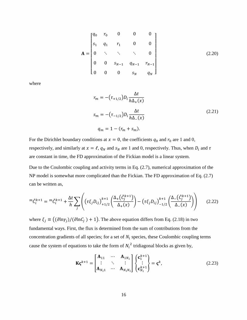
Due to the Coulombic coupling and activity terms in Eq. (2.7), numerical approximation of the

NP model is somewhat more complicated than the Fickian. The FD approximation of Eq. (2.7)

can be written as,

�̃�𝑖𝑘+1 𝑚 = �̃�𝑖𝑘+1

𝑚 +∆𝑡ℎ��𝜏𝜉𝑗𝐷𝑖𝑗�+1/2

𝑘+1�∆+��̃�𝑗𝑘+1�∆+(𝑥) � − �𝜏𝜉𝑗𝐷𝑖𝑗�−1/2

𝑘+1�∆−��̃�𝑗𝑘+1�∆−(𝑥) ��

𝑗

(2.22)

where 𝜉𝑗 ≡ �(𝜕ln𝛾𝑗)/(𝜕ln𝐶𝑗 ) + 1�. The above equation differs from Eq. (2.18) in two

fundamental ways. First, the flux is determined from the sum of contributions from the

concentration gradients of all species; for a set of 𝑁𝑖 species, these Coulombic coupling terms

cause the system of equations to take the form of 𝑁𝑖2 tridiagonal blocks as given by,

𝐊𝛓𝑘+1 = �𝐀11 ⋯ 𝐀1𝑁𝑖⋮ ⋱ ⋮

𝐀𝑁𝑖1 ⋯ 𝐀𝑁𝑖𝑁𝑖

� �𝐜1𝑘+1⋮

𝐜𝑁𝑖𝑘+1

� = 𝛓𝑘, (2.23)

17

where 𝛓 is the full set of 𝐜 vectors for each species and 𝐀𝑖𝑗 denotes a tridiagonal matrix block of

the form of Eq. (2.20). Second, the coefficient matrix 𝐊 depends upon the concentrations at the

𝑘 + 1 time step and is, consequently, nonlinear in time. Whereas a fully explicit scheme has

elsewhere been employed to model ionic transport in clays using the LEN form of the NP

equations [34-36], very small timesteps are typically required to maintain stability and accuracy

in explicit approximations of nonlinear equations. The fully implicit FD scheme, however,

allows for iterative improvement of the numerical solution and is, therefore, employed herein for

solving Eq. (2.26). Newton-Raphson iteration is implemented by defining the residual vector as

𝐫 = 𝐊𝛓𝑘+1 − 𝛓𝑘 = 0 (2.24)

Note that because 𝐊 is a linear operator on 𝛓𝑘+1, it is also the Jacobian matrix 𝜕𝐫/𝜕𝛓𝑘+1 of the

system [66]. The solution 𝛓𝑘+1,𝑠+1 is found by iteratively solving for the incremental solution at

iteration 𝑠 + 1 via

Δ𝛓 = 𝐊−1𝐫 (2.25)

and 𝛓𝑘+1,𝑠+1 = 𝛓𝑘+1,𝑠 + Δ𝛓, with calculation of the nonlinear coefficients 𝜉𝑗𝑘+1 𝑠 and 𝐷𝑖𝑗𝑘+1

𝑠 also

required at each iteration.

2.3. Model parameterization

2.3.1. Initial and boundary conditions

The material of interest is a hypothetical hydrated ordinary Portland cement (PC) with an

assumed 85% degree of reaction of each cement component, which is considered a first-order

approximation to a cement in which the C3S has been consumed. The set of primary species used

to impose mass balance in the thermodynamic equilibrium equations are chosen as the

predominant aqueous forms of the major elements present in cements. Input masses 𝑀𝑝 of the

primary species are given in Table 2.1. The aliases presented in Table 2.1, without superscripts,

are shorthand references to the primary species, 𝑝, and the dissolved concentration of a primary

species refers to the quantity 𝐶𝑝 + ∑ 𝜈𝑝𝑖𝐶𝑖𝑖≠𝑝 , that is, the portion of primary species present in

the aqueous phase.

18

Table 2.1: Masses of primary species 𝑀𝑝0 used as input to ORCHESTRA, expressed in units of

moles per liter of pore solution, for an 85% hydrated Portland cement paste.

Primary Species Alias Concentration

OH- pH

CO3-2 CO3 2.115(10-1)

NH4+ NH4 0

NO3- NO3 0

Na+ Na 4.287(10-2) Mg+2 Mg 1.601(10-1)

Al[OH]4- Al 6.086(10-1)

SO4-2 S 2.429(10-1)

Cl- Cl 4.495(10-3)

K+ K 7.222(10-2)

Ca+2 Ca 7.293

Fe[OH]4- Fe 3.445(10-1)

Three reactive transport scenarios are herein considered (Table 2.2). In the first scenario, the

external solution is deionized water (DI), in the second, a 1.5 M ammonium nitrate solution

(AN), and in the third, a 3× diluted waste form simulant porewater (WF) as measured by

porewater expression under triaxial compression [67]. These three simulated solutions have been

chosen to serve as representative cases of three general classes of leaching problems that are

determined by the composition of the external solution: very dilute solution (DI), concentrated

solution of a single electrolyte (AN), and concentrated multi-ionic solution (WF). Each leaching

scenario has practical significance as well; DI water leaching is prescribed in Method 1315 for

assessing the release of constituents of potential concern [68], AN is commonly used as an

accelerated degradation agent for the study of cement and concrete durability [69], and WF may

provide an indication of the interactions between cement waste forms and concrete

superstructures.

19

Table 2.2: Masses 𝑀𝑝0 [mol per L solution] of the primary species of the three external solutions

considered: deionized water (DI), ammonium nitrate (AN), and 3× diluted waste form porewater (WF). Masses are expressed in units of moles per liter of solution. Also shown are the calculated equilibrium pH and ionic strength values of each solution.

Primary Species DI AN WF

OH 0

CO3 0 0 3.849(10-02)

NH4 0 1.500 0

NO3 0 1.500 1.192

Na 0 0 1.473

Mg 0 0 0

Al- 0 0 0

Si 0 0 0

S 0 0 2.000(10-02)

Cl- 0 0 2.963(10-03)

K 0 0 3.978(10-02)

Ca 0 0 2.833(10-04)

Fe- 0 0 0

pH 7.00 4.62 12.48

Ionic Strength 0 1.083 1.140

2.3.2. Thermodynamic constants

Laws of mass action stability constants were computed from Gibbs free energies obtained

primarily from Lothenbach et al. [70] and the Nagra/PSI thermodynamic database [71] when

possible; however, additional values have also been obtained from Lothenbach and Winnefeld

[72], Faure [73], and Shock et al. [74]. The free energies of all aqueous species considered are

provided in Appendix A and notably include several cation-silicon complexes which have been

found to persist in geologic media [75].

The solid species included in the thermodynamic model, given in Appendix B, reflect, primarily,

those used for modeling the hydration of Portland cement, including two solid solution models of

calcium silicate hydrate (C-S-H) [72] which attempt to capture the incongruent

20

precipitation/dissolution behavior of the primary hydration phase of Portland cements.

Monosulfate (AFm), monocarbonate (AFmc), hemicarbonate (AFmhc), and ettringite (AFt) ideal

solid solutions between Al- and Fe-bearing end-members have also been included. A number of

phases that are unlikely to form in ordinary Portland cement, for instance halite and nitratine

(NaNO3 (cr)), have also been included in anticipation of their possible stability as a result of

exposure to the various external solutions. Neither sorption nor exchange reactions have been

included in the simulation, which renders Na, K, and Cl completely soluble in the native PC pore

solution. Listed in Table 2.3 are the calculated equilibrium concentrations of primary species in

the PC pore solution, using the input masses in Table 2.1 and the thermodynamic constants in

Appendices A and B.

Table 2.3: Calculated equilibrium concentrations [mol/L] of primary species in the native PC pore solution.

Primary Species PC pore solution

OH

CO3 1.004(10-04)

NH4 0

NO3 0

Na 4.116(10-01)

Mg 8.001(10-11)

Al 1.080(10-03)

Si 9.505(10-03)

S 1.516(10-02)

Cl- 4.315(10-02)

K 6.933(10-01)

Ca 2.926(10-04)

Fe- 1.115(10-05)

pH 13.89

Ionic Strength 0.910

21

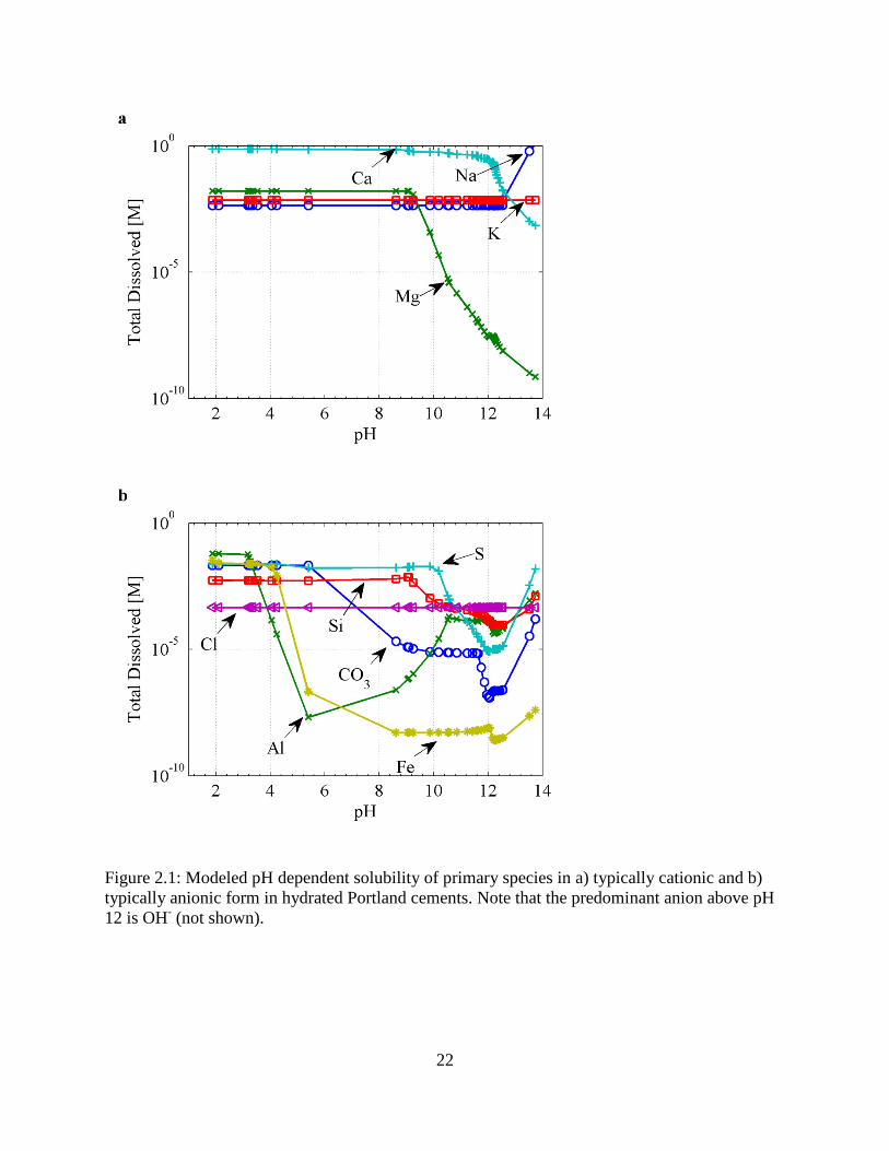
To elucidate the effects of speciation on transport behavior, the pH-dependent solubility behavior

was first simulated in the absence of ionic transport. The simulation mimicked the USEPA

Method 1313 leaching protocol [76], wherein 40 grams of dry, granular hydrated Portland

cement are added to 400 grams of deionized water and an aliquot of either NaOH or HNO3 in

order to raise or lower, respectively, the pH of the aqueous solution. The simulated pH-

dependent release curves for the major primary entities of PC are presented in Fig. 2.1, and, in

general, the solubility of primary species, excepting Na, K, and Cl, is predicted to be highly

sensitive to pH in the relevant range of pH 9 to 14, with the increase in Na solubility in the high

pH range due to the aliquot of NaOH added during Method 1313 to adjust pH. Thus, it is

expected that small differences in pH evolution predicted by the Fickian and LEN transport

models could lead to significantly different ionic fluxes in the reactive transport model. Further,

the solubilities of Mg and Ca increase monotonically with decreasing pH, whereas the

solubilities of Al, Si, and S reach a minimum solubility at pH of about 12.5. Also of significance

is that the predominant anion above pH 12 is hydroxide.

22

Figure 2.1: Modeled pH dependent solubility of primary species in a) typically cationic and b) typically anionic form in hydrated Portland cements. Note that the predominant anion above pH 12 is OH- (not shown).

23

2.3.3. Activity coefficients

In this work, the modified Davies equation developed for cementitious materials [77] has been

adopted for describing the activities of aqueous species. This model is advantageous in the fact

that it does not require parameters for individual species but instead has been optimized for

describing the ions in cement pore solutions up to and ionic strength of 1.5 M.

In the modified Davies model, the activity coefficients 𝛾𝑖 may be expressed as

ln𝛾𝑖 = −𝐴𝑧𝑖2√𝐼

1 + 𝛽𝐵√𝐼+

(𝛼𝐼 + 0.2)𝐴𝑧𝑖2𝐼√1000

, (2.26)

where 𝐼 = 12∑ 𝐶𝑖𝑧𝑖2𝑖 is the ionic strength, 𝐴 and 𝐵 are physical parameters given by

𝐴 = √2𝐹2𝑒

8𝜋(𝜖𝑟R𝑇)3/2 ,𝐵 = �2𝐹2

𝜖𝑟𝑅𝑇, (2.27)

𝜖𝑟 [C/V/m] is the relative permittivity of the solution, and 𝑒 [C/particle] is the elementary

particle charge. The coefficients 𝛼 and 𝛽 are fitting parameters which have been optimized in

[77] for describing the activities of major cement primary species with values 𝛼 = −4.17 ×

10−5 and 𝛽 = 3 × 10-10, respectively.

A commonly employed form of the NP equation (Eq. 2.6) expands the partial derivative of

logarithms as

�𝜕ln𝛾𝑖𝜕ln𝐶𝑖

� ∇𝐶𝑖 = 𝐶𝑖∇(∂ ln 𝛾𝑖). (2.28)

However, in this work it is proposed to evaluate (𝜕ln𝛾𝑖)/(𝜕ln𝐶𝑖 ) analytically which eliminates

the need to approximate ∇(∂ ln 𝛾𝑖) and the concomitant error associated with the approximation.

Using Eq. (2.26), the partial derivative of logarithms in Eq. (2.8) may then be written explicitly

as

𝜕ln𝛾𝑖𝜕ln�̃�𝑖

= −𝐴�𝑧𝑖3��2�̃�𝑖

4 �𝛽𝐵 |𝑧𝑖|√2

��̃�𝑖 + 1�2 +

𝐴𝑧𝑖4�̃�𝑖�𝛼𝑧𝑖2�̃�𝑖 + 0.2�2√1000

. (2.29)

24

Thus, 𝜕ln𝛾𝑖/𝜕ln�̃�𝑖 is evaluated analytically, and, for neutral species, it is easy to verify that

𝜕ln𝛾𝑖/𝜕ln�̃�𝑖 is always zero and 𝛾𝑖 is always one, that is, the activity is equivalent to the molar

concentration.

2.3.4. Ionic diffusion coefficient estimation

A significant hindrance to isolating the influence of the charge-coupling mechanism in the LEN

model (Eq. 2.7) is that for many of the aqueous species present in alkaline geologic media

(Appendix A) the ionic diffusion coefficient 𝐷𝑖𝑢 has not been experimentally determined.

Therefore, in the present study, the values of unknown 𝐷𝑖𝑢 have been estimated empirically as a

function of both the size and charge of the unhydrated ion. Such a functional relationship is

similar to the relationship proposed by Oelkers and Helgeson [78] who correlated 𝐷𝑖𝑢 to both the

formal charge and the effective electrostatic radius of aqueous charged species. In their model,

the diffusivity is directly proportional to the formal charge and inversely proportional to the

effective electrostatic radius, as predicted by the Stokes-Einstein relation. Such a simplistic

model belies the true complexity of ion transport; as suggested by [79] the ionic diffusivity

fundamentally depends on the tendency of the ion to break the hydrogen bonds of the loosely

structured water molecules in the vicinity of the hydrated of the ion [80]. Koneshan et al. [81]

recently investigated the structure making and breaking tendencies within a molecular dynamics

simulation of several monoatomic ions, but, to the authors’ knowledge, such a study of many of

the aqueous species studied herein, given in Appendix A, has not been undertaken. Extension of

these simulations to the ions found in cementitious media may prove to be eminently useful,

especially within the context of determining radionuclide mobilities, but at present, simple

empirical relations serve to generate feasible, albeit inaccurate, values of 𝐷𝑖𝑢.

25

Table 2.4: Ionic species used for estimation of unknown ionic diffusion coefficients. Estimated van der Waals volumes 𝑉𝑖 [Å3] and published diffusion coefficients 𝐷𝑖𝑢 [10-9 m2/s] given in [82].

Species 𝑉𝑖 𝐷𝑖𝑢 Species 𝑉𝑖 𝐷𝑖𝑢 Species 𝑉𝑖 𝐷𝑖𝑢

Al+3 33.51 1.623 HSO4- 61.95 1.385 OH- 19.54 5.273

Ba+2 33.51 1.694 I- 32.52 2.045 H2PO4- 61.80 0.959

Ca+2 33.51 1.584 IO3- 65.67 1.078 HPO4

-2 59.39 1.518 Cl- 22.45 2.032 K+ 87.11 1.957 PO4

-3 56.99 2.472

CO3-2 42.84 1.856 Li+ 25.25 1.029 Rb+ 33.51 2.072

Cs+ 33.51 2.056 Mg+2 21.69 1.412 S2O3-2 74.34 2.264

Fe+2 33.51 1.438 Mn+2 33.51 1.424 SeO4-2 69.54 2.016

Fe+3 33.51 1.812 Na+ 49.00 1.334 SO3-2 55.88 1.898

H+ 0.00 9.310 NH4+ 25.28 1.957 SO4

-2 64.34 2.130

HCO3- 42.84 1.185 NO2

- 34.16 1.912 Sr+2 33.51 1.582

HS- 27.04 1.731 NO3- 41.94 1.902 UO2

+2 48.37 0.852

Whereas Oelkers and Helgeson [78] related 𝐷𝑖𝑢 to the effective electrostatic radius, it was found

in this work that 𝐷𝑖𝑢 is more strongly correlated to the approximate van der Waals volume 𝑉𝑖

[Å3] which was calculated using the Calculator Plugins module of the chemical structure

visualization tool Marvin 6.1.3, 2013, ChemAxon (http://www.chemaxon.com). Calculated van

der Waals volumes and 𝐷𝑖𝑢 values for ions experimentally-reported 𝐷𝑖𝑢 values are provided in

Table 2.4 Cations and anions are treated as separate populations because the diffusivity of anions

appears to be far more sensitive to the ratio of charge to van der Waals volume, 𝑧𝑖/𝑉𝑖, as

demonstrated in Fig. 2.2. The form of 𝐷𝑖𝑢 expressed as a function of 𝑧𝑖/𝑉𝑖 for both cations and

anions was found using linear least squares regression. For anions, this relationship takes the

form

𝐷𝑖𝑢 = 10−9 × (−29.9 × 𝑧𝑖/𝑉𝑖 + 0.885), (1)

and for cations

𝐷𝑖𝑢 = 10−9 × (−1.92 × 𝑧𝑖/𝑉𝑖 + 1.689). (2)

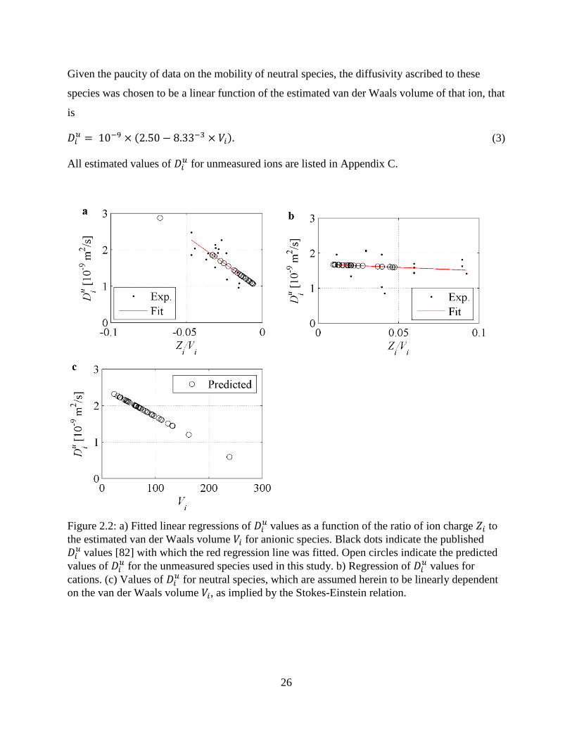
26

Given the paucity of data on the mobility of neutral species, the diffusivity ascribed to these

species was chosen to be a linear function of the estimated van der Waals volume of that ion, that

is

𝐷𝑖𝑢 = 10−9 × (2.50 − 8.33−3 × 𝑉𝑖). (3)

All estimated values of 𝐷𝑖𝑢 for unmeasured ions are listed in Appendix C.

Figure 2.2: a) Fitted linear regressions of 𝐷𝑖𝑢 values as a function of the ratio of ion charge 𝑍𝑖 to the estimated van der Waals volume 𝑉𝑖 for anionic species. Black dots indicate the published 𝐷𝑖𝑢 values [82] with which the red regression line was fitted. Open circles indicate the predicted values of 𝐷𝑖𝑢 for the unmeasured species used in this study. b) Regression of 𝐷𝑖𝑢 values for cations. (c) Values of 𝐷𝑖𝑢 for neutral species, which are assumed herein to be linearly dependent on the van der Waals volume 𝑉𝑖, as implied by the Stokes-Einstein relation.

27

2.4. Results and discussion

2.4.1. Example 1: Comparison of Fickian and LEN transport in an inert porous medium

The pertinent question for long-term performance assessment is whether the transient

concentration profiles computed from the two equations are substantially different. Previously,

Snyder and Marchand [47] found that a simple Fickian model was inadequate to describe the

migration of ions in a nonreactive porous frit subjected to various boundary conditions; however,

the counterdiffusion of ions from the boundary into the medium in their experiments is atypical

of most leaching test specifications wherein deionized water (DI) is used as leachant. Therefore,

to address the magnitude of differences between Fickian and LEN transport, a model problem

without chemical reaction is devised as follows. At 𝑡 = 0 the region from 0 ≤ 𝑥 ≤ ℓ = 0.02 m

contains an aqueous solution of 50 M each of completely dissociated Na+, Cl-, K+, OH-, Ca+2,

and SO4-2 ions in the pores, and the concentration at 𝑥 = 0 is zero for 𝑡 > 0. The fictitious

tortuosity factor of the medium is assumed to be 50. In the LEN case, the values of 𝐷𝑖 for Na+,

Cl-, K+, OH-, Ca+2, and SO4-2 were taken from published values [82] whereas in the Fickian case

the 𝐷𝑖 was set to a uniform value for all species corresponding to the unweighted mean of the six

individual diffusion coefficients, 2.649 ×10-9 m2/s. The rationale for choosing such a problem is

that, initially, the concentration gradients of all species are equal, and, therefore, any differences

in release are entirely due to variation of 𝐷𝑖𝑢 across species and to the Coulombic coupling and

activity terms of Eq. (2.7).

The concentration depth profiles and the time-dependent fluxes out of the material (at 𝑥 = 0)

after 14 days of simulation are illustrated in Figs. 2.3a and 2.3b, respectively. The shape of the

concentration curves in Fig. 2.3a varies greatly from species to species which implies that

regression of effective diffusivities for each ion using the Fickian model will depend upon

experimental conditions. It is apparent from Fig. 2.3b that in the NP model the flux of OH- is

approximately four times that of SO4-2 initially, which portends a possibly significant effect on

constituent release from the highly alkaline and largely pH-dependent PC system. Moreover,

magnitudes of primary species fluxes are ordered as OH- > K+ > Cl- > Ca+2 > Na+ > SO4-2

whereas 𝐷𝑖 are ordered as OH- > SO4-2 > Cl- > K+ > Ca+2 > Na+ such that measuring 𝐷𝑖 for a

single species and extrapolating to the others based on their 𝐷𝑖𝑢 values would be inconsistent

with the NP model prediction. In both the concentration profiles (Fig. 2.3a) and time-dependent

28

fluxes (Fig. 2.3b), the mean value of 𝐷𝑖 appears to be near-optimal in that the Fickian response

lies near the average LEN response for all ions. Nonetheless, the conclusion of this exercise is

that even in relatively simple systems, the LEN model may predict behaviors that are distinctly

“non-Fickian”.

Figure 2.3: a) Comparisons of concentration depth profiles at 7 days of simulation time. Shown are ion concentrations predicted by the LEN model: Na+ as blue asterisks, Cl- as green triangles, K+ as red “+”, SO4

-2 as cyan squares, Ca+2 as purple “x”, and OH- as gold circles. The Fickian model predicts identical releases of all ions, only one of which is shown with black bullets and denoted “Fick”. b) Estimated primary species fluxes out of the porous material (at 𝑥 = 0) as a function of root time.

Given the highly reactive nature of cementitious materials, these results are insufficient per se to

conclude that Coulombic coupling is an important factor for accurately modeling transport in

cementitious materials. Therefore, to assess the differences in the Fickian and LEN in reactive

transport modeling, the leaching of hydrated ordinary Portland cement has been investigated

using the three distinct external leaching solutions defined in Table 2.2: DI, AN, and WF. In the

Fickian transport case, the primary species diffuse at a single “mean” rate of 2.385 ×10-9 m2/s,

whereas in the LEN transport case, each aqueous species is transported with 𝐷𝑖𝑢 given in Table

2.4 and Appendix C. In the following sections, the results of these comparisons are presented by

evaluating the concentration-depth profiles of primary species, as the local concentrations of

aqueous species reflect local physico-chemical phenomena that may lead to differences in, for

instance, microstructural damage predictions.

29

2.4.2. Example 2: Dilute external leachant

Deionized water is often used to assess the leachability of constituents within solid matrices and

is prescribed in standard leaching protocols. The Fickian and LEN model predictions of primary

species concentration profiles for monolith leaching with DI are presented in Figs 2.4-2.7. In Fig.

2.4, it is apparent that the differences between models predicted for major species profiles are

minute. After 10 months of simulated leaching, the concentration profile of total dissolved Ca

exhibits a difference on the order of one percent at a depth of 1 mm, whereas pH, Al, and Si

predictions differ between the two models by less than one percent.

30

Figure 2.4: Comparison of a) pH, b) Ca, c) Al, and d) Si aqueous concentration profiles predicted by the Fickian and LEN transport models for the case of DI water leaching of PC after 280 days of simulated leaching.

31

Figure 2.5: Comparison of typically cationic primary species profiles predicted by the Fick and LEN transport models for the case of DI water leaching of PC.

The concentration profiles of Na and K in Figs. 2.5a and 2.5b demonstrate that, in both the

Fickian and LEN models, the transport of these primary species has reached steady state. Similar

to Ca, the concentration profile of total dissolved Mg, in Fig. 2.5c varies slightly at a depth of

1mm. Otherwise, the variation between model predictions is quite small. The same is true for the

primarily anionic primary species plotted in Fig. 2.6. Notably, the transport of Cl (Fig. 2.6c) has

also reached steady state, as no Cl-bearing solid phases have formed.

32

Figure 2.6: Comparison of typically anionic primary species profiles predicted by the Fick and LEN transport models for the case of DI water leaching of PC.

Illustrated in Fig. 2.7 are the predicted masses of hydrate phases per liter of control volume (Ltot),

after 280 days of simulation, and, as expected based on the dissolved primary species profiles,

only slight differences near the boundary are observed between the two models. The close

agreement between models implies that any predicted physical and mechanical properties would

likely be similar as well.

33

Figure 2.7: Mass of hydrated PC phases ( [kgsolid/Ltot]) after 280 days of simulated DI water leaching. Note that the first node at depth = 0 corresponds to the external solution.

The main finding from this exercise is that, the LEN model is slower to approach steady state

than the Fickian, but at 280 days the differences in transport models have greatly diminished.

This result can be explained through examination of the magnitudes of primary species

concentrations in Figs. 2.4-2.6; the primary ions in solution are the alkalis and OH-, each on the

order of 0.1 M. Thus, the charge coupling in the LEN model is achieved primarily through the

balance of these three ions, resulting in a system that behaves similar to the binary electrolyte

case since Na+ and K+ both possess a single positive charge.

2.4.3. Example 3: Concentrated single-salt leachant

Ammonium nitrate solution is commonly used to enhance the rate of decalcification of

cementitious materials, but its single-salt electrolyte composition makes it an informative case to

study from the perspective of charge-coupling phenomena. Results of simulated ammonium

nitrate (AN) solution leaching are illustrated in Figs. 2.8-2.13. In contrast to the case of DI

leaching, the profiles of pH, Ca, Si, and Al, profiles exhibit differences after 280 days of

simulated leaching. Although the trends in these simulations are very much the same, the region

of sharp pH depression (at ca. 5 mm depth) has progressed approximately 1-2 mm farther in the

34

Fickian model than in the LEN. Similarly, the peaks of Ca, Si, and Al concentrations are nearer

to the specimen surface in the Fickian model.

Figure 2.8: Comparison of a) pH, b) Ca, c) Al, and d) Si aqueous concentration profiles predicted by the Fickian and LEN transport models for the case of AN leaching of PC after 280 days of simulated leaching.

35

Figure 2.9: Comparison of a) ammonium and b) nitrate primary species concentration profiles predicted by the Fick and LEN transport models for the case of AN leaching of PC.

In Figs. 2.9a and 2.9b the total dissolved concentration profiles of the primary species NH4 and

NO3 are plotted, respectively. In the 10 months of simulated time, the Fickian model predicts

steady-state concentration profiles of both primary species, but in the LEN model, both NH4 and

NO3 fail to reach steady state. Moreover, the NH4 profile falls below the steady-state profile

whereas the NO3 profile falls above. To elucidate the reason for these differences, the

distributions of NH4 and NO3 species within the depth of the material after seven days of

simulation are plotted for the LEN model in Figs. 2.10a and 2.10b, respectively. Note that no

solid phases bearing NH4 or NO3 were formed during simulation. The speciation of NH4 at the

left boundary consists of only NH4+ and the ion pair NH4NO3

0. Upon entering the alkaline PC

porewater, appreciable amounts of NH30 and NH4NO3

0 form, and because these two species are

not present at the boundary, they diffuse outward. Thus, the ingress of total NH4 into the external

solution is hindered by “back diffusion” of these neutral species with the alkaline porewater

acting as a source for NH30 and NH4NO3

0. Incidentally, due to their neutrality, both species move

according to their own concentration gradient and diffusion coefficient. NO3 also forms ion pairs

with both Ca+2 and K+ within the PC porewater, but in general the distribution of NO3 within PC

porewater is more similar to its distribution at the boundary than is NH4.

36

Figure 2.10: Distribution of predominant NH4 species (a) and NO3 species(b) within the pore solution after 28 days of simulated AN leaching using the LEN model.

As demonstrated in Fig. 2.11, the profiles of primarily cationic primary species also exhibit

differences between the Fickian and LEN models. Similar to NH4 and NO3, the concentrations of

both Na and K in Figs. 2.11a and 2.11b, respectively, have not reached steady state but are

instead biased above the steady state profile. The LEN concentration profile of Mg, shown in

Fig. 2.11c, exhibits a peak that is nearer to the left boundary and two times greater in magnitude

than the Fickian model prediction.

As illustrated in Fig. 2.1, a number of primary species such as Mg and Ca exhibit solubilities that

are highly sensitive to pH in the range of 12-13. Indeed, in the AN leaching case, the solubility

of Mg has increased by six orders of magnitude due to the change in porewater pH (Fig. 2.11b).

For these primary species, the choice of transport model can exert considerable influence on

leaching behavior because the estimate of ion flux out of the material is determined by the

concentration profile near the boundary. As such, the finite difference approximation of the

gradient between the first and second nodes for Mg in Fig. 2.11b, is four times greater for the

LEN model.

37

Figure 2.11: Comparison of typically cationic primary species profiles predicted by the Fick and LEN transport models for the case of AN leaching of PC.

The concentration profiles of both CO3 and S, shown in Figs. 2.12a and 2.12b, suggest a

fundamentally similar behavior in the release of these two ions. Interestingly, the CO3 peak is

lower in the Fickian case than in the LEN, whereas the peak in S concentration near the

boundary is higher in the LEN case. Similar to the other non-precipitating species, Cl (Fig.

2.11c) has not reached steady state in the LEN model after 280 days of leaching.

38

Figure 2.12: Comparison of typically anionic primary species profiles predicted by the Fick and LEN transport models for the case of AN leaching of PC.

Fig. 2.13 illustrates the predicted total masses of hydrates along the depth profile of the PC

material, and, whereas the trends predicted by both models are quite similar, a distinct peak of

reprecipitation at half the material depth occurs approximately 2 to 3 mm farther into the

material in the Fickian model simulations at 280 of leaching. Such differences may not only

prove to be significant for the prediction of mechanical properties of degraded materials but may

also be exacerbated when the effect of porosity and tortuosity change on transport is considered.

39

Figure 2.13: Profile of the predicted mass of hydrated PC phases [kgsolid/Ltot] after 280 days of AN leaching.

The major finding of this exercise is that charge-coupling phenomena exhibit greater departures

from Fickian diffusion for the AN leaching case as opposed to the DI case, which is perhaps

indicative of greater complexity within the most abundant dissolved ions in the AN case. In

addition to the high concentrations of NH4 and NO3 primary species and of the alkalis in the

native porewater, the aqueous concentrations of dissolved Ca species increases to the order of 0.1

M in the near surface region. Satisfying electroneutrality is thus “complicated” by the presence

of the divalent Ca+2 ion as well as Ca(OH)+ and other aqueous Ca complexes and ion pairs.

2.4.4. Example 4: Concentrated multi-ionic leachant

The LEN and Fickian predictions of pH, Ca, Si, and Al concentration profiles for the case of

waste form (WF) leaching are plotted in Fig. 2.14. Despite very similar trends, the two models

exhibit slight differences in pH profile after 280 days of simulated WF leaching. The LEN model

predicts higher peak Ca and Al concentrations whereas the Fickian model predicts a Si peak four

times greater in magnitude than the LEN model prediction. A similar discrepancy is encountered

for Al except that it is the LEN model which predicts a higher Al peak concentration.

40

Figure 2.14: Comparison of concentration profiles of a) pH, b) Ca, c) Si, and d) Al predicted by the Fickian and LEN transport models for the case of WF leaching of PC.

As illustrated in Figs. 2.15a and 2.15b, the departures from steady state for Na and K predicted

by the LEN model are relatively small after 280 days of leaching. Mg concentration, on the other

hand, exhibits two distinct peaks near the specimen boundary in the Fickian model whereas the

LEN model predicts only a single peak at approximately the same location. Inspection of the

solid phases controlling Mg solubility in Figs. 2.16a and 2.16b reveals that the hydrotalcite-type

M4AH10 phase exhibits “complementary” peaks. In both transport models, M4AH10 has

reprecipitated near the boundary, but in the Fickian model, this reprecipitation peak has begun to

dissolve. In this manner, the release behavior is linked not only to Al and OH, but as shown in

41

Figs. 2.16c and 2.16d, the formation of Mg(OH)+ and MgSiO2(OH)20 further couples the

transport of Mg to OH concentration and introduces a direct dependency on the concentration of

aqueous Si.

Figure 2.15: Comparison of typically cationic primary species profiles predicted by the Fick and LEN transport models for the case of WF leaching of PC.

42

Figure 2.16: Comparison of the Mg-bearing solid phases predicted by the a) Fickian and b) LEN reactive transport models.

The predicted concentration profiles of typically anionic primary species differ very little

between the LEN and Fickian models, as demonstrated in Fig. 2.17. The concentration profiles

of the non-precipitating primary species Cl and NO3 are nearer to their steady state distributions

than in the AN leaching case but less so than in the DI leaching case. Similarly, the differences in

predicted mass of hydrates at 280 days, as shown in Fig. 2.18, are trivial between the two

transport models.

43

Figure 2.17: Comparison of typically anionic primary species profiles predicted by the Fick and LEN transport models for the case of WF leaching of PC.

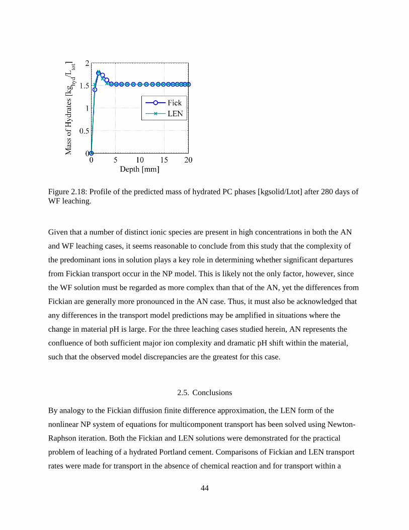
44

Figure 2.18: Profile of the predicted mass of hydrated PC phases [kgsolid/Ltot] after 280 days of WF leaching.

Given that a number of distinct ionic species are present in high concentrations in both the AN

and WF leaching cases, it seems reasonable to conclude from this study that the complexity of

the predominant ions in solution plays a key role in determining whether significant departures

from Fickian transport occur in the NP model. This is likely not the only factor, however, since

the WF solution must be regarded as more complex than that of the AN, yet the differences from

Fickian are generally more pronounced in the AN case. Thus, it must also be acknowledged that

any differences in the transport model predictions may be amplified in situations where the

change in material pH is large. For the three leaching cases studied herein, AN represents the

confluence of both sufficient major ion complexity and dramatic pH shift within the material,

such that the observed model discrepancies are the greatest for this case.

2.5. Conclusions

By analogy to the Fickian diffusion finite difference approximation, the LEN form of the

nonlinear NP system of equations for multicomponent transport has been solved using Newton-

Raphson iteration. Both the Fickian and LEN solutions were demonstrated for the practical

problem of leaching of a hydrated Portland cement. Comparisons of Fickian and LEN transport

rates were made for transport in the absence of chemical reaction and for transport within a

45

reactive hydrated Portland cement. In the case of solute transport without chemical reaction,

differences in primary species fluxes as large as a factor of two were found between the two

transport models even though the concentration gradients of all ions were initially equivalent.

Comparisons of reactive transport reveal that the trends predicted by both models are quite

similar in most cases. For deionized water leaching, no significant differences were observed

between the two transport models. For the case of ammonium nitrate leaching, however, large

departures from Fickian diffusion were observed for the LEN model due to the confluence of

charge-coupling phenomena and highly pH-dependent primary species solubilities. In

simulations of leaching with simulated waste form porewater, similar pH-dependent differences

were observed for the LEN transport model; in particular, the LEN model predicted that after

280 days of simulated leaching, several non-precipitating species failed to obtain their steady

state concentration profiles. Moreover, for the case of ammonium nitrate leaching, the uptake of

both NH4 and NO3 was predicted to have important differences, with speciation proving to be a

primary factor in determining these differences.

On the whole, comparison of the three leaching cases suggests that sufficiently complex major

ion composition and dramatic changes in porewater pH are sufficient conditions for inducing

departures from Fickian diffusion in the LEN model. These departures may have important

implications for the release of trace constituents, which may be effectively governed by the

chemistry and transport of major species in the LEN model. Furthermore, the differences

between the Fickian and LEN models are not uniformly biased for the three leaching cases

examined herein, which underscores the possibility that any regressed value of effective Fickian

diffusion coefficient may be a strong function of the conditions under which it is obtained.

46

CHAPTER 3

3. SOLUTION OF THE NONLINEAR POISSON-BOLTZMANN EQUATION:

APPLICATION TO CEMENTITIOUS MATERIALS1

Abstract

A robust numerical solution of the nonlinear Poisson-Boltzmann equation for asymmetric

polyelectrolyte solutions in discrete pore geometries is presented. Comparisons to the linearized

approximation of the Poisson-Boltzmann equation reveal that the assumptions leading to

linearization may not be appropriate for the electrochemical regime in many cementitious

materials. Implications of the electric double layer on both partitioning of species and on

diffusive release are discussed. The influence of the electric double layer on anion diffusion

relative to cation diffusion is examined.

3.1. Introduction

As the service life requirements of cementitious applications become more demanding, the need

for mechanistically based, long-term prediction of material performance grows ever more

pressing. More accurate estimation of constituent release is especially important for predicting

performance of cementitious materials in waste management applications, wherein the

cementitious matrix is relied upon to retain and/or impede migration of contaminants. Describing

ionic transport in cementitious materials is complicated by the interplay of several factors

including constituent retention via ion-exchange and adsorption, precipitation and dissolution of

solid phases, the formation of expansive products which may lead to cracking, and the movement

of ions through an often restrictive and tortuous pore space. Additional complications are

apparent at the boundaries between cementitious materials and geologic media, where dramatic

disparities in chemistry can induce large gradients in ionic composition (e.g., pH, ionic strength,

etc.). Exacerbating this complexity is the fact that, even if relatively high ionic strength cement

1 Published in Cement and Concrete Research, 44 (2013)

47

pore solution were considered in isolation, localized ion-ion and ion-solvent interactions might

still play a significant role in determining the rate of ion transport [47, 83, 84].

A further confounding effect that seems to have been obscured by the aforementioned aspects of

cement complexity is the much faster apparent diffusion of anions as compared to cations in

steady-state through-diffusion experiments. In such experiments, two parallel faces of a

cementitious specimen are exposed to two different solutions, an “upstream” solution with high

tracer concentration and a “downstream” solution with little to no tracer present. One-

dimensional diffusion subsequently occurs through the cementitious membrane due to the

concentration difference Δ𝐶𝑖 of species 𝑖 between the downstream and upstream compartments.

Observed diffusivity 𝐷𝑖𝑜𝑏𝑠 of species 𝑖 is calculated from

𝐽𝑖 = −𝐷𝑖𝑜𝑏𝑠 Δ𝐶𝑖Δ𝑥

(3.1)

where Δ𝑥 is the width of the cementitious membrane, and the flux of species 𝑖, that is, 𝐽𝑖, is

calculated from the change in concentration of 𝑖 in the downstream compartment per time

interval between measurements of 𝑖. Steady state is assumed when 𝐽𝑖 is constant after successive

measurements. Atkinson et al. found that 𝐷𝑖𝑜𝑏𝑠 for cations and anions measured in diffusion cell

experiments may differ by up to an order of magnitude with decreasing water/cement ratio[85].

Others have reported observed anion diffusivities approximately five to twenty times greater than

cation diffusivities, as demonstrated in Table 3.1 [85-88]. Such differences may become very

important when predicting the rate of ingress of corrosive species, such as chloride or sulfate,

and the rate of egress of constituents of potential concern (e.g., Tc-99 in nuclear waste

management applications).

48

Table 3.1: Apparent diffusivities reported in the literature from diffusion cell experiments on cementitious materials. Free diffusivities of Na+, K+, and Cl- in water are 1.334, 1.957, and 2.032 [10-9 m2/s], respectively [82].

𝐷𝑖𝑜𝑏𝑠 [10-12 m2/s]

Diffusivity Ratio

Reference Salt Upstream Salt Conc. [M]

Water/Cement [-]

Cation Anion Anion/Cation

[87] NaCl* 0.5 0.45 0.83 4.2 5.1

NaCl* 0.5 0.45 0.85 10.8 12.7

NaCl# 0.5 0.40 1.35 826 612

NaCl# 0.5 0.40 1.6 7.0 4.4

NaCl 0.5 0.35 1.32 6.8 5.2

[88] NaCl 1.0 0.4 0.19 3.2 16.8

NaCl 3.0 0.4 0.33 1.8 5.5

KCl 0.5 0.4 0.2 3.7 18.5

KCl 1.0 0.4 0.35 2.9 8.3

KCl 2.0 0.4 0.46 1.9 4.1

*duplicate experiments. #duplicate experiments (first case apparently in error in context of other reported data)

Observations of disparate cation/anion diffusivities coupled with measurement of significantly

high membrane potentials and zeta potentials [86, 89-91] in cementitious materials and their

constituent phases led Chatterji and Kawamura [88, 92] to suggest the electric double layer

(EDL) as the underlying cause of disparate ionic diffusivities and to propose a qualitative

description of the process. The quantitative descriptions of EDL theory are rooted in the early

20th century [93-95], and since that time, numerous investigations have aimed at illuminating

manifestations of the double layer in various materials. Of particular interest are studies of the

EDL in clays wherein anions are repelled by Coulombic forces from the negatively charged clay

surface [96-98]; the effect of this repulsion is an exclusion of ions from a fraction of the pore

space which serves to limit the area available for anion diffusion and, hence, slow anion

diffusion with respect to cation diffusion [36, 99-103]. Slower anion diffusion is precisely

opposite the observation of ionic diffusion in cement diffusion-cell through-diffusion

49

experiments despite the expectation that the surface charge of calcium-silicate-hydrate (C-S-H),

the primary solid phase of cementitious materials, is expected to be negative also at the pH of the

pore water (typically about 12.5 for ordinary Portland cements). As the surface charge of C-S-H

is determined by the amphoteric silanol site, depression of the pore solution pH could lead to a

reversal of the surface charge and cation exclusion, but this situation is unlikely given the

buffering capacity of Portland cement systems.

Due to the complexity of cementitious materials in both composition and in pore space

morphology, a number of factors in addition to EDL effects may be fully or partially responsible

for enhanced anion diffusion in cementitious materials. Unfortunately, a full mechanistic

description of disparate ionic diffusivities originating from EDL phenomena in cementitious

materials has yet to be developed; a first step toward such a description is the modeling of the

EDL. Typically, the effects of the EDL are addressed through a simplified version of the

Poisson-Boltzmann equation (PBE), the Gouy-Chapman formulation, which is valid for low

ionic strength symmetric systems with symmetric electrolyte composition, that is, every cation of

the bulk solution with valence +𝑧 is accompanied by an anion of valence of −𝑧. Recently,

Friedmann et al. [104] have demonstrated the effects of the EDL on transport in simple pore

geometries using the analytical solution of the PBE and assuming a symmetric electrolyte

composition of the pore solution, a condition that need not hold in real systems.

The objective of the research presented here is to develop and use a numerical solution of the full

nonlinear PBE for the purposes of modeling the electric double layer for asymmetric non-dilute

pore water compositions of cements. For the sake of conceptual and computational simplicity,

pore boundaries in this work are envisaged as uniformly charged cylinders or parallel plates;

however, a primary advantage of the finite difference solution is that it is extensible to arbitrary

pore geometries provided that the pore boundary is sufficiently smooth. The pore water

composition and pore size distribution of a blended cementitious mortar were measured in order

to demonstrate the possible effects of the EDL on diffusion in a model cementitious material.

Solutions of the PBE are used, then, to ascertain 1) the degree of divergence of the linear and

nonlinear solutions for expected conditions in cementitious materials and 2) whether the effect of

the EDL on diffusion may be significant for the relevant range of pore sizes encountered in

cementitious materials.

50

3.2. Experimental Methods

3.2.1. Sample preparation

Structural vault concrete (SVC) samples were prepared by mixing ordinary Portland cement,

blast furnace slag, coal fly ash, water, and quartz sand in the proportions listed in Table 3.2,

resulting in a water-to-binder (w/b) ratio of 0.45. The formulation of SVC is within the family of

compositions used as vault concretes in nuclear waste management applications [1]. SVC

specimens were cast into cylindrical molds with 10.2 cm diameter and 20.4 cm height.

Specimens were unmolded after 24 hours, and allowed to cure at 98 ± 2% relative humidity and

20 ± 2°C for 60 days.

Table 3.2: Proportion of mix components, in mass percent.

Component Mass %

BFS 8.0

FAF 16.9

OPC 5.40

QS 55.0

Water 14.6

3.2.2. Pore water expression

Expression of pore liquid from saturated SVC cylindrical specimens was performed by SIMCO

Technologies, Inc. (Québec City, Québec, Canada) according to the triaxial compression method

set forth by Barneyback and Diamond [105]. Pore solution was collected and analyzed for

chemical composition of Cl- and OH- using potentiometric titration, and for Ca+2, Na+, K+ and

SO4-2 using inductively coupled plasma optical emission spectroscopy [106].

51

3.2.3. Porosimetry

Two porosimetry techniques were performed on crushed and vacuum-dried mortar samples.

Mercury intrusion porosimetry (MIP) was conducted by Micrometerics (Norcross, GA, USA)

using a 15 second pressure equilibration time and an assumed mercury contact angle of 130º,

resulting in an “intrusion diameter” distribution of pores ranging from approximately 400 µm to

4 nm in diameter. Two intrusion cycles were executed sequentially in order to determine the

volume of “ink-bottle” pores (pores connected to the mercury accessible porosity only via a

smaller pore), within the specimen [107]. Nitrogen adsorption/desorption experiments were

performed on vacuum-desiccated specimens using a Micromeritics ASAP (Accelerated Surface

Area and Porosimetry System) 2010. Pore size distribution and pore volume of pore diameters

between 2 to 600 nm were calculated using the BJH (Barret, Joyner, and Halenda) model applied

to both adsorption and desorption isotherms. An estimate of specific surface area was also made

using Brunauer-Emmett-Teller theory applied to the nitrogen adsorption isotherm [108].

Additionally, ASTM procedure C 642 [109] was performed to quantify water-accessible, or

“total”, porosity and bulk density.

3.3. EDL modeling

Adsorption of ions onto solid surfaces induces a gradient in electrical potential 𝜓 [V] near the

solid-pore liquid interface of charged porous media. The excess surface charge due to adsorbed

species must be balanced by the presence of counter-ions in a “diffuse swarm” in the near-

surface region, and these two regions are collectively referred to as the electric double layer

(EDL). The interdependence of the diffuse layer charge density 𝜌𝐷 [C/m3] and 𝜓 gives rise to the

elliptic partial differential equation termed the Poisson-Boltzmann equation:

∇2𝜓 = −𝜌𝐷ϵ0ϵ

(3.2)

where ϵ0 is the permittivity of free space [8.854 x 10-12 C/V/m], ϵ is the dielectric constant of the

solution [-], and ∇2 is the Laplace operator. Concentration of a particular species at a distance 𝑥

[m] normal to a solid surface depends upon the energy state of that species and is therefore given

52

by the Boltzmann distribution. Thus, 𝜌𝐷 is simply the difference in positive and negative charge

distributions for all species 𝑖, such that

𝜌𝐷 = 𝑒NA�𝑧𝑖𝐶𝑏,𝑖exp �−𝑧𝑖𝑒𝜓

kB𝑇� ,

𝑖

(3.3)

where 𝐶𝑏,𝑖 is the concentration in the bulk pore solution [mol/m3], 𝑒 is the elementary

electrostatic charge [C/particle], NA is Avogadro’s number [particles/mol], and kB is the

Boltmann constant [J/K] [110]. For small distances from a charged surface and for very large

values of 𝜓, the Boltzmann distribution runs into difficulties because it may predict impossibly

high values of concentration of ions given their finite sizes , however, this problem is alleviated

by limiting the number of near surface charges to a maximum determined by the number of

available “adsorption” sites within the near-surface region of finite thickness termed the “Stern

layer” [111]. For the purposes of this work, the effects of the Stern layer are not taken into

account explicitly; rather, it is assumed that the thickness of the Stern layer is negligible as

compared to the width of the pores in question and that balancing of the structural charge by the

Stern layer is negligible such that the effective potential boundary condition to be solved, 𝜓𝑏𝑐, is

equivalent to the potential of the outer Helmholtz plane 𝜓𝛿 [112]. Moreover, the systems

considered are assumed to be open such that the bulk concentrations 𝐶𝑏,𝑖 are constant values

which implies that masses of ions in the EDL are negligible compared to the bulk concentrations.

Combining Eqs. (3.2) and (3.3) yields the general form of the full nonlinear PBE:

∇2𝜓 = −𝑒NA

ϵ0ϵ�𝑧𝑖𝐶𝑏,𝑖exp �

−𝑧𝑖𝑒𝜓kB𝑇

� .𝑖

(3.4)

Eq. (3.4) may be linearized if 𝑧𝑖𝑒𝜓 ≪ kB𝑇, that is, where the electrical potential energy of an ion

(𝑧𝑖𝑒𝜓) is small compared to its thermal energy (kB𝑇), such that

∇2𝜓 = 𝜅2𝜓 (3.5)

where 𝜅2is the Debye parameter, given as [94]

𝜅2 =𝑒2NA

ϵ0ϵkB𝑇�𝐶𝑏,𝑖𝑧𝑖2𝑖

. (3.6)

53

Eq. (3.4) is by far the most commonly employed version of the PBE; however, electrophoretic

measurements of hydrated cement and its constituent solid phases indicate that the magnitude of

the electrokinetic (zeta) potential (which we assume approximates the potential of the Helmholtz

plane, 𝜓𝛿) for cement is typically on the order of tens of millivolts, in which case the exponential

terms may not be neglected [89, 92]. In systems for which linearization of the PBE is not

appropriate, simplification of Eq. (3.4) is still possible with the assumption that the system is

comprised of a single symmetric electrolyte, that is, for every cation of valence +𝜁 there exists

an anion of valence – 𝜁. Assuming symmetry, the exponentials of Eq. (3.4) may be combined to

yield

∇2𝜓 = −2𝑒NA

𝜖0𝜖𝜁𝐶𝑖sinh �

𝜁𝑒𝜓kB𝑇

� (3.7)

for which analytical solutions are possible; however, experimental evidence indicates that

constituents of real cementitious pore solutions are unlikely to be symmetric or of a single

valence [113].

The full nonlinear PBE only assumes that the configuration of charges in proximity to a charge

surface follows a Boltzmann distribution and may be solved numerically as follows. The left

hand side of Eq. (3.4) is replaced by a second order central finite difference, and the exponential

on the right hand side is expanded as the infinite Taylor series:

exp(𝜉) = �𝜉𝑛

𝑛!

∞

𝑛=0

= 1 + 𝜉 + �𝜉𝑛

𝑛!

∞

𝑛=2

(3.8)

with 𝜉 = −𝑧𝑖𝑒𝜓 kB𝑇⁄ . Thus, the exponential function may be subdivided into a linear part, 𝜉,

and a nonlinear part, 1 + ∑ 𝜉𝑛

𝑛!∞𝑛=2 . Solution of Eq. (3.4) then follows closely the method

proposed by Nicholls and Honig [114] excepting that electrolyte symmetry was not assumed.

The value of potential at given node, 𝜓0, is expressed as a function of the values of 𝜓 at the

nearest neighboring nodes, the constant term, and the power series of 𝜉

𝜓0 = �� 𝜓𝑘𝑎𝑙𝑙 𝑘

+ �𝑒NA

ϵ0ϵ� 𝑧𝑖𝐶𝑏,𝑖 �1 + �

𝜉𝑛

𝑛!

∞

𝑛=2

�𝑎𝑙𝑙 𝑖

� ℎ2� �� 1𝑎𝑙𝑙 𝑘

+ 𝜅2ℎ2�� , (3.9)

54

where 𝑘 represent the indices of the six nearest neighbors [(𝑥 − 1,𝑦, 𝑧), (𝑥 + 1,𝑦, 𝑧), … ] and ℎ is

the grid spacing [m]. For a discretization of 𝐿3 nodes, Eq. (3.9) may be written in vector notation

as

𝚿𝑡+1 = T𝚿𝑡 + 𝐐 (3.10)

where 𝚿𝑡+1 is the 𝐿 × 1 vector of 𝜓 values computed at the next iteration 𝑡 + 1, 𝚿𝜏 are the 𝜓

values at the current iteration 𝑡, T is an 𝐿 × 𝐿 matrix of coefficient values, and 𝐐 is the vector of

nonlinear terms. Successive “under relaxation” is applied to Eq. (3.10), and the nonlinearity 𝐐 is

treated as a perturbation of the solution [114]. To maintain stability, 𝐐 is scaled by a factor 𝜔𝑸

that grows with each iteration; for example:

𝜔𝑸 = �0.5𝑡 for 𝑡 ≤ 201 for 𝑡 > 20 . (3.11)

The final iteration algorithm is written as

𝚿𝑡+1 = 𝜔ΨT𝚿𝑡 + (1 − 𝜔Ψ)𝚿𝑡 + 𝜔𝑸𝐐 (3.12)

where 𝜔Ψ is the relaxation parameter. Dirichlet boundary conditions (𝜓𝑏𝑐 = constant) are

imposed at the pore wall corresponding to the potential just beyond the Stern layer, assumed

herein to be approximated by the zeta potential. Periodic boundary conditions are imposed at the

“ends” of a pore, and values of 𝜓 are then computed from Eq. (3.12) until the maximum change

in 𝜓 is less than a specified tolerance, here 10-4 mV. Once satisfactory convergence of the

solution has been obtained, the concentration of any particular ion may be computed from the

Boltzmann distribution

𝐶𝑖 = 𝐶𝑏,𝑖 exp �−𝑧𝑖𝑒𝜓

kB𝑇�. (3.13)

The solution scheme was implemented in the commercial computational software package

MATLAB (MATLAB 7.10.0, The MathWorks Inc., Natick, MA, 2000).

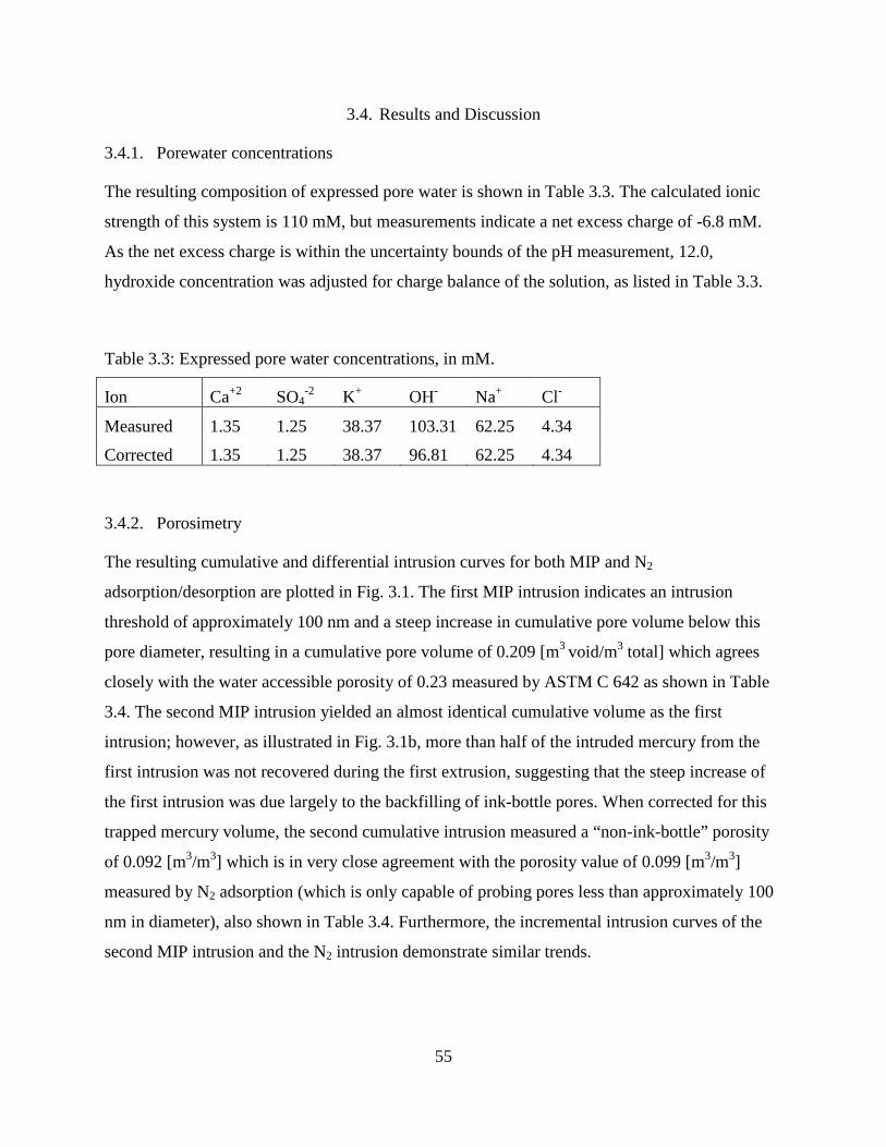
55

3.4. Results and Discussion

3.4.1. Porewater concentrations

The resulting composition of expressed pore water is shown in Table 3.3. The calculated ionic

strength of this system is 110 mM, but measurements indicate a net excess charge of -6.8 mM.

As the net excess charge is within the uncertainty bounds of the pH measurement, 12.0,

hydroxide concentration was adjusted for charge balance of the solution, as listed in Table 3.3.

Table 3.3: Expressed pore water concentrations, in mM.

Ion Ca+2 SO4-2 K+ OH- Na+ Cl-

Measured 1.35 1.25 38.37 103.31 62.25 4.34

Corrected 1.35 1.25 38.37 96.81 62.25 4.34

3.4.2. Porosimetry

The resulting cumulative and differential intrusion curves for both MIP and N2

adsorption/desorption are plotted in Fig. 3.1. The first MIP intrusion indicates an intrusion

threshold of approximately 100 nm and a steep increase in cumulative pore volume below this

pore diameter, resulting in a cumulative pore volume of 0.209 [m3 void/m3 total] which agrees

closely with the water accessible porosity of 0.23 measured by ASTM C 642 as shown in Table

3.4. The second MIP intrusion yielded an almost identical cumulative volume as the first

intrusion; however, as illustrated in Fig. 3.1b, more than half of the intruded mercury from the

first intrusion was not recovered during the first extrusion, suggesting that the steep increase of

the first intrusion was due largely to the backfilling of ink-bottle pores. When corrected for this

trapped mercury volume, the second cumulative intrusion measured a “non-ink-bottle” porosity

of 0.092 [m3/m3] which is in very close agreement with the porosity value of 0.099 [m3/m3]

measured by N2 adsorption (which is only capable of probing pores less than approximately 100

nm in diameter), also shown in Table 3.4. Furthermore, the incremental intrusion curves of the

second MIP intrusion and the N2 intrusion demonstrate similar trends.

56

Table 3.4: Results of ASTM C 642 density and water accessible porosity determination, mercury intrusion porosimetry (MIP), and N2 adsorption (N2 Ads.).

ASTM C 642 MIP N2 Ads.

Bulk density, dry [g/cm3]

Bulk density, saturated [g/cm3]

Porosity [m3/m3]

Porosity,

1st Intrusion [m3/m3 ]

Porosity,

2nd Intrusion [m3/m3]

Porosity

[m3/m3]

BET specific surface area [m2/g]

1.96 2.19 0.23 0.209 0.092 0.099 8.63

Figure 3.1: Cumulative intrusion volume (a), and differential intrusion volume (b) for MIP intrusion cycles 1 (open circles) and 2 (filled circles), and for N2 adsorption (open triangles) and N2 desorption (filled triangles).

Both porosimetry techniques suggest a finer pore structure than typically encountered for

ordinary Portland cement (OPC). Whereas the median pore diameter of OPC generally lies on

the order of 100 nm, the median diameter of the mortar as measured by N2 adsorption is on the

order of 50 nm. Of the four porosimetry curves, N2 adsorption yields the smallest amount of fine

pore volume and was therefore chosen as a bounding estimate of the smallest likely fraction of

fine pores. A beta distribution was fit to the probability density function derived from the

incremental N2 adsorption, as shown in Fig. 3.2, and summary statistics from this fit are listed in

Table 3.4.

57

Figure 3.2: Experimentally determined N2 adsorption incremental volume curve (N2 Ads) and a beta distribution fit (Fit) to the curve.

Table 3.5: Statistics computed from the beta distribution fit to the N2 adsorption incremental volume curve. Percentiles (pct.) indicate the percentage of the volume comprised of pores less than or equal to the given diameter [nm].

mean std. dev 25th pct. 50 th pct. 75 th pct.

58.6 7.8 23.4 47.5 83.0

3.4.3. EDL Modeling

For solution of the PBE, it is assumed that in a given pore, the surface potential is isotropic and

the populations of species within the pore are constant. Aqueous ionic species are assumed to

remain fully ionized, and chemical reactions including surface adsorption/desorption are not

allowed to occur. Although the solution to the PBE is given for a single pore, the solution may be

regarded as an average over all pores of a given size.

It is assumed that cylindrical pore boundaries may be reasonably approximated with a fine

rectangular grid spacing, in this case 106 nodes. In order to avoid the trivial solution of constant

𝜓 at all nodes for symmetric electrolytes, the initial values of 𝜓 were set to zero at all nodes,

save the boundary conditions; thus, the incremental solution of Eq. (3.9) was guaranteed to pass

through the nontrivial solution.

58

3.4.3.1. Academic examples

The behavior of the nonlinear PBE can be illustrated with a hypothetical cylindrical pore

measuring 10 nm in diameter with a uniform and constant surface potential. A zeta (boundary)

potential value of -25 mV was chosen as a reasonable estimate for cementitious materials based

on reported measured values [115]. The pore is filled with an electrolyte solution comprised of

an arbitrary cation M+m and anion A-n. Three illustrative cases are presented herein. In Case 1,

the pore is saturated with a 100 mM solution of symmetric monovalent or 1:1 electrolyte solution

(e.g., MA). In Case 2, the pore is filled by a 100 mM asymmetric 1:2 electrolyte solution (e.g.,

MA2) with a resultant ionic strength of 300 mM. For the last case (Case 3), the pore is filled with

an asymmetric 1:2 electrolyte solution at 33 mM. Thus, Cases 1 and 2 both possess a cation

concentration of 100 mM while Cases 1 and 3 both have an ionic strength of 100 mM. The

potential profiles and cation/anion concentration profiles extending radially from the pore for all

three cases are presented in Fig. 3.3 (a-c). Shown in the plots are the potential distribution (a) and

ion distribution (b and c) for all three cases. Plot d) shows the deviations between the linear and

nonlinear mean pore potentials (expressed as percent difference between the linear and nonlinear

solution, that is 100% ∗ (|𝜓𝑙𝑖𝑛𝑒𝑎𝑟 − 𝜓𝑛𝑜𝑛𝑙𝑖𝑛𝑒𝑎𝑟|)/𝜓𝑛𝑜𝑛𝑙𝑖𝑛𝑒𝑎𝑟) as a result of varying surface

potential for the porewater concentrations of all three cases.

Fig. 3.3d reflects the difference in the linear and the nonlinear solutions, which is proportional to

∑ exp(−𝑧𝑖𝑒𝜓 𝑘𝐵𝑇⁄ ). Accordingly, the difference reaches a minimum for vanishing 𝜓, and

increases for increasing 𝜓, tending toward a maximum when 𝑧𝑖 and 𝜓 are opposite in sign.

Assuming an asymmetric solution may be approximated by a symmetric monovalent solution

leads to deviations which are apparent in the comparison of Case 1 (symmetric) and Case 2

(asymmetric) in Fig. 3.3d; the difference in mean potential for the symmetric and asymmetric

cases is as much as 15% for a large surface potential.

59

Figure 3.3: Simulated potential profiles for a 10 nm wide pore with constant surface potential of -25 mV and pore solutions of 100 mM MA (Case 1),100 mM MA2 (Case 2), and 33mM MA2 (Case 3), where M and A denote cations and anions, respectively. Shown are plots of potential distribution (a) and ion distribution (b,c) as a function of distance from the pore wall for all three cases. Shown in d) are deviations between the linear and nonlinear mean pore potentials (expressed as percent difference between the linear and nonlinear solutions) as a result of varying surface potential for the porewater concentrations of all three cases.

A number of observations are apparent from the comparison of the solution of the full nonlinear

PBE for all three cases, shown in Fig. 3.3a - 3.3c The spatial extent of the diffuse layer is greater

for Case 1 than Case 2, as the divalent M+2 ion can more efficiently neutralize the surface charge

than the monovalent A- ion. This neutralization occurs in spite of the molar concentration of A-

being twice the value of Case 1 and, as indicated in Eq. (3.3), is due to the linear dependence of

local concentration on bulk concentration and an exponential dependence on the square of the

valence state. The potential profiles for Cases 1 and 3 are nearly identical, yet the relative

increase in M+2 concentration as compared to the bulk in Case 3 is significantly higher than the

M+ increase in Case 1. In all three cases, anion concentrations decrease markedly in the vicinity

60

of the surface charge. Therefore, with decreasing pore diameter, mean anion concentrations

within a pore diminish while mean cation concentrations increase. Considering diffusion through

one such pore and assuming the Boltzmann distribution holds in the presence of a concentration

gradient, a few deductions may be made:

The net flux of cations through the pore will be determined by the combined effects of electrical

retardation through interaction with the anionic surface layer (decreasing local intrinsic cation

diffusivity) and of increased local concentrations of cations that serve to increase the diffusion

gradient. The cross-sectional area available for anion diffusion will be reduced due to electrical

repulsion from the anionic surface layer, thereby reducing the anion flux as compared to flux

through a pore with an uncharged surface layer. In well-connected pore networks, the reduced

area for anion flux should serve to reduce the observed diffusivities of anionic species.

If the pore diameter is small enough relative to the thickness of the EDL, anions will be excluded

from the pore. Thus, small pores may serve to limit the accessibility of not only pores but pore

pathways to anions. In well-connected pore networks, this phenomenon should also be expected

to reduce observed diffusivity of anions; however, in poorly-connected networks, that is those

containing many dead-end pores, the anion-specific tortuosity could be significantly reduced if

the pore pathways from which anions are excluded are highly tortuous.

3.4.3.2. Application to blended cement mortar

The trends observed from rudimentary examples are, nonetheless, persistent in simulations of the

more complex pore solution specified in Table 3.3. A surface potential of -25 mV was chosen as

a plausible value for a hydrated cement system based upon electrokinetic measurements found in

the literature [92, 104, 116, 117]. A useful metric for comparing the impact of the EDL on a

particular species is the mean pore concentration, 𝐶𝑖,𝑎𝑣𝑔 [mM], which for a cylindrical pore with

radius 𝑟𝑝 [nm] is computed as the integral over the cross-sectional area of the pore

𝐶𝑖,𝑎𝑣𝑔 =2𝑟𝑝2� 𝑟𝐶𝑖(𝑟)𝑑𝑟.𝑟𝑝

0 (3.14)

The ratio of total positive dissolved charges to total negative charges ∑𝑧𝑖+𝐶𝑖,𝑎𝑣𝑔+ �∑ 𝑧𝑖−𝐶𝑖,𝑎𝑣𝑔− ��

(neglecting charges of the adsorbed ions), also gives an indication of the relative influence of the

61

EDL. Fig. 3.4 depicts mean pore solution concentrations 𝐶𝑖,𝑎𝑣𝑔 required to maintain

electroneutrality within a pore normalized by the bulk concentration 𝐶𝑏,𝑖 for a range of pore

diameters relevant for cementitious materials. Also, plotted in Fig. 3.4d is the charge ratio for

diffusing ions in solution. As expected, the concentration-altering, anion-excluding effect is

exacerbated by both decreasing pore diameter and decreasing ionic strength, resulting in

significant departures from bulk concentrations. At the ionic strength of the pore solution for the

unleached mortar, approximately 5% of the connected pores possess at least twice as many

positive charges as negative charges, whereas at a 10x dilution of the pore water (analogous to

reductions by leaching), approximately 15% of the pores have a charge ratio of at least 2; at 100x

dilution, this percentage increases to approximately 50% of the pores. The implications of these

findings are discussed next.

Figure 3.4: Normalized ion concentrations for variable pore diameters for a) the expressed pore solution, b) a 10x diluted pore solution, and c) a 100x diluted pore solution. d) The ratio of total

62

positive charge to total negative charge is calculated as ∑𝑧𝑖+𝐶𝑖,𝑎𝑣𝑔+ �∑ 𝑧𝑖−𝐶𝑖,𝑎𝑣𝑔− �� , where + and − denote cation and anion species, respectively.

3.4.3.3. Interpretation of diffusion cell experiments

The Fick’s law formulation of Eq. (3.1) belies the complexity of multicomponent ionic diffusion

in a porous medium, wherein the flux is more rigorously characterized by the Nernst-Planck

equation applied to porous materials [40]

𝐽𝑖 = 𝜏𝜙 �−𝐷𝑖𝑢∇(𝐶𝑖) −𝐷𝑖𝑢𝑧𝑖F

R𝑇𝐶𝑖∇(𝜓) − 𝐷𝑖𝑢𝐶𝑖∇(ln 𝛾𝑖)� (3.15)

where 𝜙 is the connected porosity available for diffusion [m3/m3], the tortuosity 𝜏 (≤ 1) [m/m]

characterizes the distance that an ion traverses within the pore space, 𝐷𝑖𝑢 [m2/s] is the free liquid

diffusivity of species 𝑖 at infinite dilution, 𝑧𝑖 is the valence state of species 𝑖, R is the ideal gas

constant [J/mol/K], and 𝛾𝑖 is the chemical activity coefficient of species 𝑖 [84]. In the bulk pore

solution, intermolecular forces exerted between freely moving ions ensure an equilibrium

orientation of ions such that electrical potential 𝜓 remains zero throughout; however, as

demonstrated previously, the potential near charged surfaces need not be zero. Because Eq.

(3.15) is computationally taxing for realistic pore geometries on meaningful length scales, it is

rarely solved in its full form. Instead, diffusion is most often simplified to a Fick’s law

formulation with various correction terms included; to compare these different formulations, it is

convenient to cast Eq. (3.15) in terms of correction factors:

𝐽𝑖 = 𝑓𝐶𝑖(𝑓𝜏𝜏)(𝑓𝜙𝜙)

𝑓𝑖𝑅�−𝐷𝑖𝑢∇(𝐶𝑖) −

𝐷𝑖𝑢𝑧𝑖𝐹R𝑇

𝐶𝑖∇(𝜓) − 𝐷𝑖𝑢𝐶𝑖∇(ln 𝛾𝑖)� (3.16)

where 𝑓𝜙, 𝑓𝜏, and 𝑓𝐶𝑖 are corrections to the values of 𝜙, 𝜏, and 𝐶𝑖, respectively, and the factor

𝑓𝑖𝑅 represents corrections to the flux due to chemical reactions (most often assumed to be

adsorption reactions) of the diffusing species. The observed diffusivity may then be written as

𝐷𝑖𝑜𝑏𝑠 = 𝑓𝐶𝑖𝑓𝑠𝑓𝜏𝑓𝜙

𝑓𝑖𝑅𝐷𝑖𝑢𝜏𝜙. (3.17)

where 𝑓𝑠 represents the transform of the concentration-, potential-, and activity-gradient terms of

the modified Nernst-Planck equation to single scalar value. Thus, Eq. (3.17) presents a

63

framework for evaluating possible mechanisms of disparate cation/anion diffusivities and will be

used to assess whether any one correction factor can account for the half an order of magnitude

disparity between observed cation and anion diffusivity.

The possibility that the chemical reaction factor for diffusing ions, 𝑓𝑖𝑅, gives rise to disparate

cation/anion diffusivities cannot be completely dismissed without intimate knowledge of the

chemical properties of the cementitious system, although such an effect should be negligible at

steady state. The plausibility of whether a particular type of reaction could result in

𝑓𝑐𝑎𝑡𝑖𝑜𝑛𝑅 𝑓𝑎𝑛𝑖𝑜𝑛𝑅⁄ ≥ 5, however, is considered. Precipitation of the diffusing species is unlikely

given the generally high solubility of the species used in the diffusion cell experiments (K+, Na+,

Cl-), but adsorption-type reactions of these ions have been widely reported. Uptake of alkalis is

generally considered to occur as an adsorption onto the silanol sites of C-S-H [118] or as an

interlayer occupation of the calcium-alumino-silicate-hydrates (C-A-S-H) [119]. The fraction of

alkali incorporated during initial mixing is quite high and increases for low-calcium cements ,

but the partitioning of alkalis occurring into hydrated C-S-H is within a factor of two of the

reported adsorption partitioning of chloride [120, 121]. Therefore, it is doubtful that 𝑓𝑖𝑅 differs

by a factor of five or more between species.

The phenomenon of anion exclusion is well documented for charged clay soils [97, 98, 122], and

has been interpreted using the concept of an effective porosity , that is 𝑓𝜙𝜙𝑚, wherein anions are

confined to a fraction of the total porosity due to repulsion from the negatively charged pore

wall. Thus, anionic concentrations are higher in the central region of the pore resulting in a

higher diffusion gradient than would be indicated by macroscopic measurements of

concentration. An estimate of the anion-excluded pore volume, which ignores overlapping

diffuse layers, may be calculated by multiplying the Debye length (~ 1 nm for the solution given

in Table 3.3) by the pore surface area (~10 m2/g, Table 3.4), yielding an anion-excluded volume

on the order of 10% of the total porosity and an 𝑓𝜙 equal to 0.90 and which decreases 𝐷𝑖𝑜𝑏𝑠 by

10%. This crowding of anions into the central regions of pores is necessarily accompanied by a

rise in anion concentration (although the simulations presented herein give no indication that the

resulting anion concentration should be higher than in the bulk solution due to the form of the

PBE). Therefore, 𝑓𝐶𝑖 for anions in this system would be calculated as 1.11 such that the factors

𝑓𝐶𝑖 and 𝑓𝜙 would cancel one another, ruling out anion crowding as the primary origin of

64

disparate diffusivities in this particular cement mortar. Not only are the magnitudes of these

factors too small to account for a factor of five difference in diffusivities, ascribing a

macroscopic correction factor derived from microscale arguments neglects the inherent

variability of the pore space. Moreover, the utility of such a formulation has been questioned,

inasmuch as the excluded volume will depend strongly on the ionic strength of the pore solution

which may also exhibit quite significant local variation.

Because of the variation of ionic diffusion coefficients for dissolved ionic species, the electrical

coupling among species in the bulk solution, through the term (𝐷𝑖𝑢𝑧𝑖𝐶𝑖 F)/(R𝑇)∇𝜓, serves to

accelerate the movement of slower ions and retard the movement of faster ions, such that the

ratio of 𝑓𝐶𝑙𝑠 𝑓(𝑁𝑎,𝐾)𝑠� between species should be at a maximum equal to the ratio of their free liquid

diffusivities, which for the species considered is approximately a factor of 2 [43, 82]. Snyder and

Marchand [47] demonstrated that 𝐷𝑖𝑜𝑏𝑠 in nonreactive porous frit is only weakly dependent on

concentration gradient in systems of ionic strength comparable to cement pore solutions. It is,

therefore, unlikely that electrical coupling between ions could give rise to disproportionate rates

of ion transport in the bulk solution. Within the EDL, however, the electric potential may have a

strong effect on the transport of ions, and in solutions of low ionic strength, Coulombic

interactions may indeed be the dominant factor in determining transport rate. Chatterji and

Kawamura [92] argued that a high cation flux in the EDL could be the driving factor for

disparate diffusivities if the cation flux were accompanied by an accelerated anion flux (in order

to maintain charge balance) in the central region of the pore. No such mechanism is apparent

from the analytical solution of the Nernst-Planck for an idealized pore given by Friedmann et al.

[104]; rather, the ratio of cation to anion flux was found to be equivalent to the ratio of cation

charge to anion charge within a pore [104]. This formulation of the Nernst-Planck, however,

neglects the concomitant change in potential gradient in the presence of a concentration gradient.

What is apparent from the simulations of the EDL presented herein is the relatively large fraction

of porosity impacted by EDL effects. Considering that pores less than 23.4 nm constitute

approximately 25% of the total pore volume measured by N2 adsorption (Table 3.5), the

probability that any percolating pathway traverses a pore with a mean charge ratio altered by a

factor of approximately five (Fig. 3.4d) is necessarily quite high, resulting in pore “bottle-

necking” as depicted in Fig. 3.5b. Thus, a fraction of the pore space may act as a filter,

65

facilitating passage of cations and deterring the passage of anions. Consistent with observations

in clays, this assertion seems to suggest a faster diffusivity of cations (contrary to experimental

observation in cements) in that the area available for anion diffusion is less than that for cations,

that is 𝑓−𝜙 < 𝑓+𝜙. The resolution to this paradox may lie in the different percolation paths to

which cations and anions have access. Given any collection of connected pores, anion exclusion

renders more paths accessible to cations than anions, but a number of these paths are necessarily

“dead-end” or highly constricted paths in that they are only connected to the capillary porosity

network via a highly constricted opening that can selectively exclude specific ions (e.g., Cl-). In

the transient case, the loss of cations to dead-end pores may lead to an apparent retardation of

cations until the transport through the highly tortuous pathways also reaches steady state. It is

possible that the one and two week durations of the through-diffusion tests of [88] and [87],

respectively, were not long enough to capture the steady-state transport of cations through the

highly-restricted diffusion regimes. In addition, a fraction of the cations in larger pores may be

selectively diverted to more constricted pores prior to release to the downstream compartment of

the diffusion cell, resulting in an apparent reduction in the net diffusion rate of cations relative to

anions.

Another consequence of filtering effect of small connecting pores is that a fraction of pore water

anions may be trapped within ink-bottle pores (Fig. 3.5b) as a consequence of initial cement

hardening initially present in the material within ink-bottle pores may be only slowly leachable

(more slowly than cations) due to the filtering effect of small connecting pores, that is, the

macroscopic anion-specific tortuosity may be increased (i.e., a trapping effect occurring as a

consequence of initial material formation, Fig. 3.5b). In such a situation, the degree to which

anion transport from external sources appears more rapid relative to cations would depend

largely on the proportion of ink-bottle pores within the system. For clays this proportion may be

greatly influenced by the level of compaction [123] and therefore makes more difficult the

interpretation of diffusion data in the absence of pore size distribution measurements. However,

considering that, for the mortar presented, more than half of the pore volume measured by

mercury intrusion can be attributed to ink-bottle pores, the effect of such filtering pores on

overall diffusivity may be significant in this and analogous cementitious systems.

66

Furthermore, as shown in Figs. 3.4 and 3.6, the anion exclusion effect is magnified for pore

solutions diluted by factors of 10 and 100, respectively.

Although the interpretation of the continuum-representation PBE should be interpreted with

extreme caution in very dilute and transient systems, the trends from the solution of the PBE

compare favorably with molecular dynamics simulations and density-functional theory

simulations with decreasing ionic strength [124]. Thus, the PBE solution may give insight into

expected behaviors of an “average” pore. One such insight is the enhancement of anion

exclusion in dilute pores which is a very important result with respect to constituent leaching. As

pores near the leaching boundary become more dilute, the coulombic forces resulting from the

charged surface are exerted over a greater distance within those pores. Hence, a greater number

of pores exhibit significantly altered charge ratios, and the likelihood that any percolating path

contains one or more pores with significantly altered charge ratio necessarily increases. Thus, it

is possible and indeed likely that these near-surface, depleted pores have a disproportionately

large effect on the rate of constituent release.

Figure 3.5: a) Depiction of the 3-d bottle-necking pore and delineation of the boundary conditions, and b) schematic indicating the more tortuous cation path and the local distribution of anions when considering ink-bottle pores.

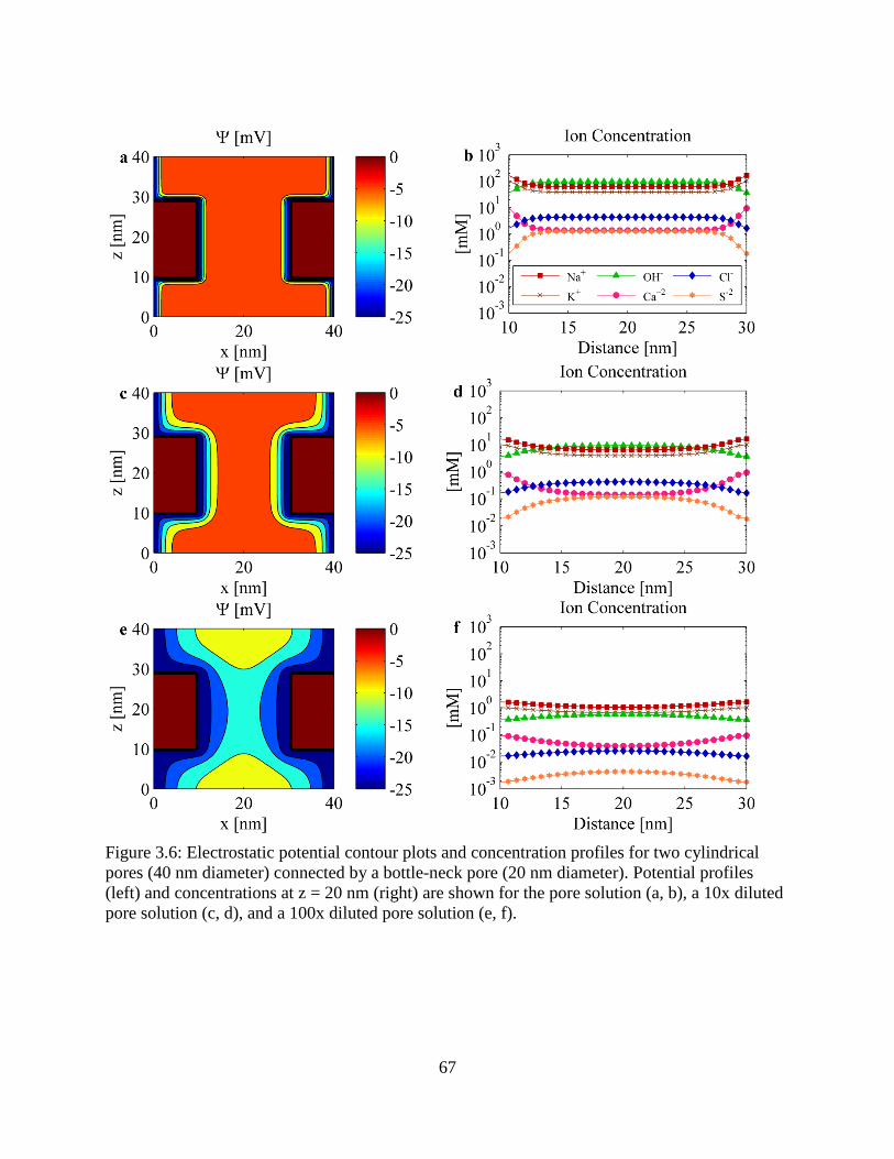
67

Figure 3.6: Electrostatic potential contour plots and concentration profiles for two cylindrical pores (40 nm diameter) connected by a bottle-neck pore (20 nm diameter). Potential profiles (left) and concentrations at z = 20 nm (right) are shown for the pore solution (a, b), a 10x diluted pore solution (c, d), and a 100x diluted pore solution (e, f).

68

3.5. Conclusions

A solution of the full nonlinear Poisson-Boltzmann equation for non-ideal aqueous solutions and

highly charged surfaces was introduced. Discrepancies between the simplified linear solution and

full nonlinear solution of as much as 50% were illustrated. Errors encountered from using the

symmetric solution of the PBE were less pronounced, ranging up to 15% for the scenarios

presented. The full nonlinear PBE solution was demonstrated for a real cementitious mortar with

known pore water composition and pore size distribution. For the relevant pore sizes of the

material, the effects of the EDL were found to alter mean ionic concentrations by at least 10%

for approximately 10% of the total connected pore volume and by as much as 500% for pores

less than 1.5 nm in diameter, resulting in a mean charge ratio for the interconnected porosity of

approximately 1.10 [|+ charge / - charge|]. Assessment of the possible mechanisms of disparate

cation and anion diffusivities suggest that anion-exclusion from poorly connected pore pathways

could lead to an apparent lower diffusivity of cations. Due to the high volume of dead-end

porosity within cementitious specimens, significant differences in anion diffusivity are

anticipated depending on whether the anion source is initially present within the material or is

introduced from an external source. Implicit in this assertion is the assumption that capillary

pores determine the rate of transport through the material; however, the importance of the small

(~1.5 nm) interlayer gel porosity and surficial phenomena cannot be immediately discounted a

priori. In addition to Coulombic forces, the effects of ion-pore, ion-solvent, and ion-ion

interactions become increasingly important with decreasing pore size. Therefore, further work

invoking solution of the coupled Nernst-Planck Poisson-Boltzmann equation, molecular

dynamics simulations, and more refined microstructural characterization of the pore space is

necessary both to substantiate these claims and ultimately to develop mechanistic-based

predictions of ionic diffusivity at the macroscale.

69

CHAPTER 4

4. BACKSCATTERED ELECTRON MICROSCOPY AND ENERGY DISPERSIVE X-RAY

ANALYSIS FOR QUANTIFICATION OF THE REACTED FRACTIONS OF

ANHYDROUS PARTICLES IN A BLENDED CEMENT MORTAR

Abstract

A novel technique is presented for the identification of unreacted binder particles in a blended

cement mortar using backscattered scanning electron microscopy (BSEM) coupled with energy

dispersive X-ray (EDX) analysis. Segmentation of unreacted particles from hydrate phases is

achieved through nonparametric global thresholding of the backscattered electron (BSE)

micrograph grayscale histogram coupled with fuzzy inference rules incorporating both textural

and EDX information. Linear discriminant analysis (LDA) is then used to differentiate between

particles according to elemental composition. Reacted fractions of anhydrous binder phases, used

for the parameterization of chemical and physical properties of cement systems, are deduced

from the difference between original and remaining area fractions of binder materials. After 30

months of curing, the Portland cement is found to be completely reacted, whereas approximately

83% of the slag and 36% of coal fly ash are reacted over that duration; these fractions are within

the range of reacted fractions for similar materials reported in the literature.

4.1. Introduction

Supplementary cementitious materials (SCMs) have been employed extensively due to their

ability to enhance mechanical performance and reduce permeability of grouts and concretes,

while providing a beneficial use for industrial byproducts and lowering the carbon footprint of

cement-based construction. A key parameter for describing the physical and chemical behaviors

of cementitious materials is the rate at which binder materials are consumed as the cement

evolves due to continued hydration and environmental aging [13]. For neat ordinary Portland

cement (OPC) pastes, consumption of the majority of clinker mass occurs within the first month

of hydration; however, the rate of reaction of SCMs may be orders of magnitude slower than that

70

of OPC. Thus, the physical and chemical behaviors of blended cement systems may at long times

be governed by the continued rate of SCM reaction.

To this end, significant progress has been made toward quantifying the reacted fraction of SCMs

in cementitious materials via segmentation of backscattered scanning electron (BSE)

micrographs [125-128]. Because the frequency with which materials elastically scatter electrons

depends upon the product of mean atomic number and density of the material, 𝑍𝑎𝑣𝑒𝜌, these

methods are able to distinguish between typically low- and high-density hydrous and anhydrous

phases, respectively, using BSE micrograph grayscale intensity. Such quantification methods

perform well for systems in which compositional differences between hydrous and anhydrous

phases are sufficiently large; however, in systems containing two or more SCMs and/or

aggregate materials [128], distinctions on the basis of BSE intensity become difficult if these

anhydrous particles possess similar values of 𝑍𝑎𝑣𝑒𝜌. This difficulty is realized for the material

pertinent to the present study, a multi-component blended cement mortar containing ordinary

Portland cement, coal combustion fly ash, ground granulated blast furnace slag, and fine

aggregate, which is similar to the vault concretes used for radioactive high-level waste tanks [1,

129].

The objective of this work is the development of a method for identifying anhydrous particles on

the basis of elemental composition obtained through energy dispersive X-ray spectroscopy

(EDX) in conjunction with BSE microscopy. Previous methods for integrating BSE-EDX

analysis into particle identification have incorporated a decision tree analysis technique, which

entails defining heuristics for classifying particles based on major element concentrations [130,

131]. In highly heterogeneous materials, constructing such a decision tree may be impossible

when distinct materials exhibit sufficiently similar compositions. The method used in the present

study differs significantly from previous approaches. First, rather than considering EDX

information pixel by pixel, pixels are grouped into particle regions in a novel segmentation step

that integrates BSE intensity, textural measures, and EDX spectra using fuzzy inference rules.

Creating particle regions in this manner ensures both spatial and compositional correlation

among the pixels in a given region. All pixels within the region are therefore assumed to be

samples of a single underlying mean composition, which effectively increases the total number

of X-ray counts, ergo precision, associated with a single composition measurement. Grouping

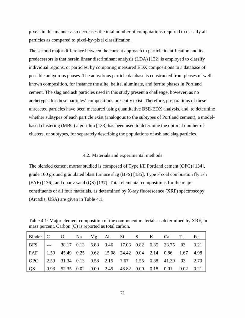
71

pixels in this manner also decreases the total number of computations required to classify all

particles as compared to pixel-by-pixel classification.

The second major difference between the current approach to particle identification and its

predecessors is that herein linear discriminant analysis (LDA) [132] is employed to classify

individual regions, or particles, by comparing measured EDX compositions to a database of

possible anhydrous phases. The anhydrous particle database is constructed from phases of well-

known composition, for instance the alite, belite, aluminate, and ferrite phases in Portland

cement. The slag and ash particles used in this study present a challenge, however, as no

archetypes for these particles’ compositions presently exist. Therefore, preparations of these

unreacted particles have been measured using quantitative BSE-EDX analysis, and, to determine

whether subtypes of each particle exist (analogous to the subtypes of Portland cement), a model-

based clustering (MBC) algorithm [133] has been used to determine the optimal number of

clusters, or subtypes, for separately describing the populations of ash and slag particles.

4.2. Materials and experimental methods

The blended cement mortar studied is composed of Type I/II Portland cement (OPC) [134],

grade 100 ground granulated blast furnace slag (BFS) [135], Type F coal combustion fly ash

(FAF) [136], and quartz sand (QS) [137]. Total elemental compositions for the major

constituents of all four materials, as determined by X-ray fluorescence (XRF) spectroscopy

(Arcadis, USA) are given in Table 4.1.

Table 4.1: Major element composition of the component materials as determined by XRF, in mass percent. Carbon (C) is reported as total carbon.

Binder C O Na Mg Al Si S K Ca Ti Fe

BFS --- 38.17 0.13 6.88 3.46 17.06 0.82 0.35 23.75 .03 0.21

FAF 1.50 45.49 0.25 0.62 15.08 24.42 0.04 2.14 0.86 1.67 4.98

OPC 2.50 31.34 0.13 0.58 2.15 7.67 1.55 0.38 41.30 .03 2.70

QS 0.93 52.35 0.02 0.00 2.45 43.82 0.00 0.18 0.01 0.02 0.21

72

4.2.1. Sample preparation

Samples of both the component SCM materials, BFS and FAF, and of the blended mortar were

prepared for BSE-EDX analysis. Approximately 20g of BFS and FAF powders were first oven

dried at 65°C for 48 hours to remove any residual moisture, then immersed in low-viscosity

methacrylate resin. The powder-resin mixtures were held under vacuum for one hour in order to

displace any air pockets with the samples.

Blended mortar samples (denoted SVC) were prepared by mixing OPC, BFS, FAF, and QS in

the proportions listed in Table 4.2; this formulation is within the family of compositions used as

structural concretes in nuclear waste management applications, with the exception that no coarse

aggregate is present in SVC [1]. SVC samples were cast as slabs measuring approximately 15 cm

width × 30 cm length × 5 cm height. Slabs were unmolded 24 hours after casting and were cured

at 98% relative humidity and 298K for 30 months in a nitrogen atmosphere. Following curing,

cylinders were cored from the slabs using a low-speed, diamond-embedded drill bit. Disks were

then sawn at low speed from the interior portion of the specimen to avoid sampling from molded

surfaces.

Table 4.2: Mix design of the blended cement mortar studied herein. Particle sizes were determined from information provided by [138].

Component Specific Gravity

Mean Particle Diameter [μm]

Median Particle Diameter [μm] Mass % Vol. %

BFS 2.89 3.87 8.12 8.0 5.8

FAF 2.33 6.02 14.90 16.9 15.1

OPC 3.01 4.16 11.30 5.40 6.0

QS 2.54 590.6 596.45 55.0 45.0

Water 1.00 - - 14.6 30.4

After coring and sawing, reaction was arrested by immersing the SVC disks in 99.5% reagent

grade ethanol for two weeks to allow for complete exchange of accessible pore water with

ethanol. Alcohol-exchanged samples were then immersed in a low-viscosity methacrylate resin

for an additional two weeks to allow for displacement of the ethanol by resin.

73

Resin-immersed samples of FAF, BFS, and SVC were hardened with a 24-hour cure at 65° C

under anoxic conditions. Samples infused with hardened resin were mechanically ground using a

sequence of 240 and 600 grit silicon carbide papers, cleaning the sample surface with ethanol

after each grinding sequence to remove any loosened debris. The samples were then

mechanically polished using two separate alcohol-based suspensions of diamond particles

possessing both 6 μm and 1 μm nominal diameters. After the final polishing step, samples were

sonicated in acetone for 20 seconds to remove any remaining debris. Samples were then

evaporatively coated with approximately 15 nm of graphitic carbon.

4.2.2. Scanning and processing

All scans were performed using a Phillips/FEI Quanta 650 field emission electron microscope

under high vacuum at 10 keV accelerating voltage and a nominal 3.5 spot size, the parameter

governing the diameter of the electron beam. BSE micrographs were obtained using the 4

quadrant solid-state BSED backscatter detector, and EDX spectra were collected using the

Oxford X-Max 50 mm2 Si(Li) X-ray detector. All BSE and EDX analyses were performed at a

working distance of 10 mm with the horizontal field of view width (HFW) set to 256 μm

(Polaroid magnification of 496x). EDX composition maps across the entire field of view were

collected with a pixel resolution of 256 x 224 such that the pixel edge length equaled 1 μm. For

each EDX map acquisition, 2000 raster frames were collected, each with a pixel dwell time set to

100 μs. The HFW was chosen as a compromise between the ability to resolve small features and

the time demand of collecting a representative number of samples. Furthermore, as will be

discussed in the next section, the resolution of the electron beam itself is on the order of 1 μm.

The sampling strategy itself was also impacted by the presence of sand particles because picking

a random sampling point on the specimen surface frequently resulted in a sand particle covering

the entire field of view. Executing a full EDX analysis for a sand particle does not provide any

information as to the hydration of the cement, slag, and ash particles; therefore, sampling points

were chosen using a Latin hypercube sampling of the unit disk [139] and then shifted to the

nearest non-sand area to maximize sampling efficiency. In total, 12 preparations each of BFS and

FAF particles and 12 preparations of SVC monoliths were analyzed.

74

4.2.3. Sources of experimental uncertainty

In addition to the usual uncertainties associated with experimental measurements, such as

accuracy of calibration and variation of experimental conditions, a few sources of uncertainty

specific to BSE-EDX analysis warrant further discussion here. The extent to which useful

compositional information may be gleaned from a BSE micrograph is limited by the topographic

variation of the specimen surface, which may give rise to darker and lighter regions that obscure

the underlying compositionally-dependent backscattering efficiency of the material. Such

variations are observable in the BSE micrographs of the mechanically polished SVC because of

the variation in hardness among the sand, hydrates, and anhydrous particles. Small (2002)

demonstrated the magnitudes of topographic errors across a range of accelerating voltages using

spherical analytical glass standards; measurements on resin-mounted and polished glass shards

reveal a relative error in mass fraction measurement on the order of 10% with an excitation

voltage of 10 keV to values between 25 and 60% with an excitation voltage of 25 keV.

Therefore, given the 10 keV excitation voltage used in this study, the errors associated with

topographic variation are expected to be small.

An essential component of the quantitative analysis of heterogeneous materials is delineating the

region from which the signal originates. Although electron microscopes are capable of producing

an electron beam on the order of nanometers in width, the volume in which electron collisions

occur, that is, the interaction volume, is considerably larger in most materials. For high-vacuum

SEM, Kanaya and Okayama [140] derived a semi-empirical expression for the depth of

interaction volume in pure materials, 𝑑𝐾𝑂 [μm], that is directly proportional to the excitation

voltage of the electron beam 𝐸0 [keV] and inversely proportional to atomic number, 𝑍, and to the

mole density, 𝜌 𝐴⁄ :

𝑑𝐾𝑂 = 0.0276𝐴𝐸0

5 3⁄

𝑍8/9𝜌, (4.1)

where 𝐴 is atomic mass [g/mol] and 𝜌 is the density of the medium [g/cm3]. The exponential

dependence of 𝑑𝐾𝑂 on accelerating voltage suggests that 𝐸0 should be minimized; however, the

optimal value of 𝐸0 is constrained by the requirement for sufficient BSE compositional contrast

and sufficient X-ray generation rates. For the carbon-coated samples used in this study, an

excitation voltage of 10 keV was found to yield good peak separation in the BSE grayscale

75

histogram and near the recommended X-ray collection rate (approximately 3000 counts per

second for the Oxford X-Max 50 detector). Whereas Eq. (4.1) provides an indication of size of

interaction volume for pure elements, a more rigorous characterization can be achieved by

simulating the flight paths of incident electrons, wherein the probabilities of elastic and inelastic

scattering are governed by effective atomic cross-sectional areas [141]. Using Monte Carlo

simulations of electron trajectories in cementitious targets, Wong and Buenfeld [142] estimated

the interaction volume in ettringite to be on the order of 1-100 μm3 for 𝐸0 ranging from 10-20

keV. Considering that the densities of the anhydrous particles in this study are greater than that

of ettringite, a 1 μm diameter of the interaction volume may be treated as a conservatively large

estimate for all anhydrous particles of interest herein.

The importance of estimating the interaction volume is due to the effect of partial volume

averaging (PVA). PVA occurs when the observable interaction volume, herein referred to as the

“probe” volume, is greater than the volume of the feature of interest, and in the case of particles

embedded in a resin medium, the sum of elemental mass fractions probed by the electron beam,

neglecting the contribution from the resin, is necessarily less than unity. In such situations,

renormalization of the mass fractions may be appropriate, but in scenarios in which a particle is

interspersed within a medium of comparable composition, for instance anhydrous particles

within C-S-H, PVA may lead to a locally measured composition that is characteristic of neither

the particle nor the medium. Moreover, the extent of the interaction volume will be greater in the

direction of the phase with lower mean Z due to the lower occurrence of electron scattering

events. Consequently, the fraction of pixels near a feature boundary will determine whether a

feature’s composition can be accurately measured; features smaller than the interaction volume

cannot be probed in isolation; whereas, the mean composition of very large features is relatively

insensitive to PVA of the boundary pixels. Therefore, the likelihood of misclassifying particles

smaller than the interaction volume may be high, and it is necessary to estimate the proportion of

these particles relative to the entire population.

76

Figure 4.1: a, b, and c) Probability density function representation of particle size (diameter) distributions for BFS, FAF, and OPC particles, respectively, as measured by laser diffraction of particles suspended in propan-2-ol [138]. Darker regions of each histogram to the left of the diameter on the x-axis indicate the fraction of particles smaller than the nominal probe diameter at the corresponding value. Note that the abscissa is presented on the logarithmic scale. d) Summary of the probability that a particle is smaller than the nominal probe diameter.

With an estimate of the approximate diameter of the interaction volume, the fractions of

anhydrous particles smaller than the probe volume (and necessarily partial-volume averaged)

may be calculated from particle size distributions of the isolated, unreacted binder particles

measured via laser diffraction [138]. For the BFS, FAF, and OPC particles used this study, Figs.

4.1a - 4.1c illustrate the measured distribution of particle diameters, with shaded areas

representing the fraction of particles with diameters less than or equal to the nominal probe

diameters of 1, 2, 4, and 10 μm (marked on the abscissas). As noted in Table 4.2, the mean

values of particle diameter are substantially lower than the medians for all three particles, and for

all three particle types, the maximum of the probability density function lies below the 1 μm

77

threshold. Ostensibly, the large proportion of small BFS, FAF, and OPC particles would suggest

that SEM-EDX analysis is ill-suited to characterizing these particles; however, as shown in Fig.

2.1d, particles less than 1 μm in diameter only comprise about 5 % of each unreacted material’s

population, and would be expected to comprise a much smaller fraction of the material’s

population after reaction. Thus, PVA is not deemed to be a significant source of error in

estimating the area fractions of remaining unreacted particles within the SVC mortar.

4.3. Particle identification method

Image analysis and data processing were performed using the Matlab computing environment

(MATLAB 8.1.0.604, The MathWorks, Natick, MA). Section 3.1 outlines the process of particle

identification which consists of two parts, beginning with the isolation of “anhydrous” particle

regions in a segmentation step. A binary image consisting of anhydrous and non-anhydrous parts

is constructed from the segmented image, and individual anhydrous particles are then defined as

contiguous pixels within the binary region. Defining particles in this manner ensures a priori

correlation in both spatial proximity and in compositional contrast; however, the reason for pixel

grouping is twofold: considering groups of pixels not only increases the number of X-ray counts

associated with a particle, thereby lowering the variance for a given measurement, but also

reduces the number of computations required in the classification step. The second step of the

process entails the identification of each region by comparing each particle’s composition to a

reference particle composition database. Unfortunately, no such database currently exists for the

anhydrous particles of interest, so in Section 3.2, a database is created from measurements of the

elemental compositions of isolated, unreacted BFS and FAF particles using BSE-EDX analysis.

Section 3.3 gives the details of how particles are compared to the database using the discriminant

analysis classification technique. Fig. 4.2 provides an overview of the data flow through the

overall classification strategy.

78

Figure 4.2: Data flow diagram of particle identification algorithm implemented in this work. The path designated “SCMs” describes the process for building the anhydrous particle database for subtypes of the binder materials. The path designated “Mortar” describes the process for comparing anhydrous regions identified in the hydrated SVC material to the anhydrous particle database in order to classify the anhydrous regions.

4.3.1. Segmentation

As indicated in Fig. 4.2, the segmentation procedure of SCM BSE monographs is distinct from

that of the mortar segmentation procedure, but both methods make use of the nonparametric

histogram segmentation procedure of Delon et al. [143], which shall hereafter be referred to as

DDLP (Delon, Desolneuw, Lisani, Petro). Since DDLP is used extensively in this work and has

apparently not been applied to cementitious BSE monographs previously, it is briefly outlined

next.

79

Generalized nonparametric histogram segmentation: DDLP does not require an assumption of

the number, relative fraction, or distribution type of each underlying class. Rather, each class

need only be unimodal, that is, increasing then decreasing over an interval. For any given

discrete histogram with frequency ℎ defined on the discretized domain [0, 𝐿], the set of image

thresholds 𝑆 ∈ [0, 𝐿] with indices 𝑛 ∈ [1,𝑁𝑆] is initially defined as all the local minima of ℎ,

including ℎ(0) and ℎ(𝐿). According to DDLP a candidate threshold 𝑆(𝑛) is chosen at random; in

this work, however, 𝑆(𝑛) is chosen as the threshold for which the variance of the interval

ℎ([𝑆(𝑛 − 1), 𝑆(𝑛 + 1)]) is a minimum for all possible values of 𝑛, so as to render the method

reproducible. The interval is said to be unimodal if there exists a trial threshold bin 𝑡 ∈

�𝑆(𝑛 − 1), 𝑆(𝑛 + 1)� for which no significant rejection of the unimodal hypothesis exists, and

the unimodal hypothesis is essentially that the values in ℎ(𝑎, 𝑡) are increasing and the values in

ℎ(𝑡 + 1, 𝑏) are decreasing. For each trial 𝑡, the Grenander estimator is constructed using the

“pool adjacent violators” algorithm (PAVA) for which the algorithm is provided in Appendix A

[144]. The PAVA constructs a monotonically nondecreasing estimator of the histogram interval

ℎ(𝑎, 𝑡), or, conversely, the monotonically nonincreasing estimator of ℎ(𝑡 + 1, 𝑏). An example of

the Grenander estimator for a typical histogram segment is illustrated in Fig. 4.3a. If the

subinterval ℎ(𝑎, 𝑏) is deemed to be unimodal, the threshold 𝑆(𝑛) is removed from the set of 𝑆

and the process is repeated until no more thresholds can be removed, or equivalently, until no

two adjacent segments of ℎ can be joined. The entire process is then repeated by testing for

unimodality of 3, 4 … 𝑁𝑆 adjacent segments. The output of the DDLP algorithm is the set 𝑇 of

all thresholds identified for ℎ.

SCM segmentation procedure: The efficiency with which electrons are elastically scattered by a

given element is described by the backscatter coefficient 𝜂 for that element and the

backscattering efficiency 𝜀𝐵𝑆 [-] which varies with both electron beam energy and atomic

number 𝑍 [145]. Thus, composition-dependent information is manifest within the BSE grayscale

intensity histogram and provides a semi-quantitative basis for discriminating between resin and

particle in the case of BFS, FAF, and OPC, and between resin, “hydrous”, and “anhydrous”

segments in the case of the SVC mortar [125, 146]. The terms “hydrous” and “anhydrous” here

denote only a general distinction which relies on the fact that cement hydration products

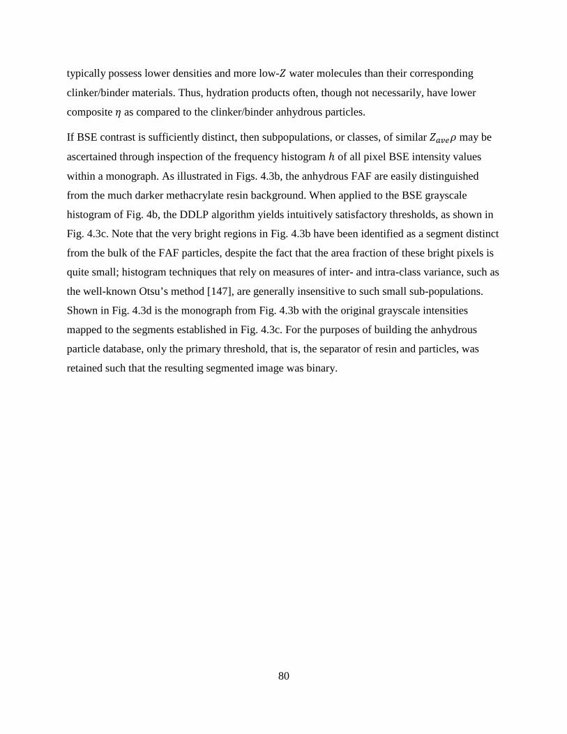
80

typically possess lower densities and more low-𝑍 water molecules than their corresponding

clinker/binder materials. Thus, hydration products often, though not necessarily, have lower

composite 𝜂 as compared to the clinker/binder anhydrous particles.

If BSE contrast is sufficiently distinct, then subpopulations, or classes, of similar 𝑍𝑎𝑣𝑒𝜌 may be

ascertained through inspection of the frequency histogram ℎ of all pixel BSE intensity values

within a monograph. As illustrated in Figs. 4.3b, the anhydrous FAF are easily distinguished

from the much darker methacrylate resin background. When applied to the BSE grayscale

histogram of Fig. 4b, the DDLP algorithm yields intuitively satisfactory thresholds, as shown in

Fig. 4.3c. Note that the very bright regions in Fig. 4.3b have been identified as a segment distinct

from the bulk of the FAF particles, despite the fact that the area fraction of these bright pixels is

quite small; histogram techniques that rely on measures of inter- and intra-class variance, such as

the well-known Otsu’s method [147], are generally insensitive to such small sub-populations.

Shown in Fig. 4.3d is the monograph from Fig. 4.3b with the original grayscale intensities

mapped to the segments established in Fig. 4.3c. For the purposes of building the anhydrous

particle database, only the primary threshold, that is, the separator of resin and particles, was

retained such that the resulting segmented image was binary.

81

Figure 4.3: a) An example of the Grenander estimator constructed for a union of two histogram segments (red and blue bars, purple indicates the overlapping segment). The increasing estimator is designated with the right-pointing green triangles, and the decreasing estimator with left-pointing magenta triangles. The test interval is marked with a vertical stripe (cyan). b) A backscattered electron image of FAF particles mounted in acrylic resin. c) Histogram of BSE intensity values of the image in b) with red lines indicated the thresholds determined by DDLP. d) The segmented BSE monograph from b) using the thresholds defined in c).

Mortar segmentation procedure: For the SVC material, differences in grayscale intensity alone

proved insufficient to segment the hydrous and anhydrous phases; quite commonly, the fine

aggregate particles used in this study exhibit lower backscatter intensities than the gel phase. For

such a highly heterogeneous material in both scale and composition, most general strategies,

such as global histogram segmentation, fail to yield meaningful results. Therefore, the goal of the

segmentation algorithm developed in this work is to “divide and conquer”. Using both BSE

intensity and textural information and EDX spectral information, the most easily segmented

82

regions are first identified and then removed from subsequent analysis so that the quantities

being analyzed at each step belong only to the remaining unclassified pixels.

The segmentation algorithm begins by enhancing features in the BSE intensity image 𝐼 using a

smoothing filter based on the 2D diffusion equation, first proposed in [148]. Denoting the

grayscale intensity at the point (𝑖, 𝑗) as 𝐼𝑖,𝑗, the smoothed image at iteration step 𝑘 + 1 is given

by the forward Euler finite difference approximation of the 2D diffusion equation

𝐼𝑖,𝑗𝑘+1 = 𝐼𝑖,𝑗𝑘 + 𝛽��𝑐𝐷∇𝐷𝐼𝑖,𝑗𝑘 �𝐷

(4.2)

where 𝛽 is a parameter equal to 1/7 for numerical stability of the explicit finite difference

scheme and 𝐷 denotes the direction of the finite difference gradient approximation, that is

𝐷 ∈ [𝑁𝑜𝑟𝑡ℎ − 𝑆𝑜𝑢𝑡ℎ,𝐸𝑎𝑠𝑡 −𝑊𝑒𝑠𝑡,𝑁𝑜𝑟𝑡ℎ𝐸𝑎𝑠𝑡 − 𝑆𝑜𝑢𝑡ℎ𝑊𝑒𝑠𝑡, 𝑆𝑜𝑢𝑡ℎ𝐸𝑎𝑠𝑡 − 𝑁𝑜𝑟𝑡ℎ𝑊𝑒𝑠𝑡].

The authors of the original algorithm referred to the filtering scheme as “anisotropic” diffusion

because the diffusion coefficients 𝑐𝐷 depend directly upon the magnitude of the gradient in

image intensity at the previous timestep. For this work, 𝑐𝐷 have a Gaussian-type functional form

proposed in [148] given by

𝑐𝐷𝑖,𝑗𝑘 = 𝑔��∇𝐷𝐼𝑖,𝑗𝑘 �� = exp�−�

�∇𝐷𝐼𝑖,𝑗𝑘 �𝑊

�2

�. (4.3)

Thus, the effect of this scheme is to smooth most in the direction of the gradient where gradients

are strongest and to smooth very little along contours such as edges. The total number of time

levels and the parameter 𝑊 are adjustable scaling parameters in time and space, respectively,

which have been set to 50 and 0.05 at the authors’ discretion. Using Eqs. (4.2) and (4.3), the

intensity image 𝐼 is smoothed and normalized to the interval [0,1] to yield the matrix 𝐼∗ that

generally exhibits a histogram with more pronounced separations of peaks. The DDLP algorithm

is applied to the histogram of 𝐼∗ to yield a set of 𝑁 preliminary threshold values 𝑆𝐼 which are

used to create a segmented map, 𝐼𝐿∗, of 𝑁 − 1 levels 𝐿.

The difficulty with treating 𝐼𝐿∗ as the final segmented map is that in the 30 month cured mortar

studied herein, areas of the gel phase exhibit a very high BSE intensity. In order to distinguish

between these areas and anhydrous particles, the disordered nature of the gel phase is exploited;

the gel’s lack of ordered structure on the micrometer scale leads to a high variation in local

83

values of 𝐼. Thus, the Gaussian smoothed gradients 𝐺𝑥 and 𝐺𝑦 of 𝐼∗ are computed in the x and y

dimensions, and the classical texture metric 𝐺 is defined as

𝐺 = �𝐺𝑥 + 𝐺𝑦�. (4.4)

With textural information in hand, the next step in the segmentation procedure is to march

through the levels of 𝐼𝑆∗ and examine whether the pixels belonging to each level are high gradient

or low gradient areas. For this purpose, the DDLP algorithm is employed once again, but because

𝐺 is a measure of the change in approximately Gaussian variables, it is necessary to perform

DDLP on the histogram of the natural logarithm Γ = ln (𝐺). The histograms of Γ computed are

used to compute the set 𝑆Γ(ℓ) of thresholds for each level ℓ:

𝑆Γ(ℓ) = DDLP�Γ ⨂𝐻(𝐼𝐿∗ = ℓ)�, ℓ ∈ 𝐿 (4.5)

where 𝐻(∙) denotes the element-wise Heaviside function, that is

𝐻(𝑥) = �0, 𝑥 < 01, 𝑥 ≥ 0 (4.6)

and ⨂ denotes element-wise multiplication. Almost invariably, the histograms of Γ for each level

are strongly bimodal, such that 𝑆Γ(ℓ) contains three members per level, and the primary

threshold 𝑡Γ(ℓ) is simply the median value of the set 𝑆Γ(ℓ). Proceeding from the brightest level

in 𝐼𝐿∗, a binary map of anhydrous particles with low gradient values, 𝐵𝑚𝑎𝑝, is constructed

recursively as

𝐵𝑚𝑎𝑝 = 𝐵𝑚𝑎𝑝 ∪ 𝐻�Γ < 𝑡Γ(ℓ)� ⨂𝐻(𝐼𝐿∗ = ℓ), (4.7)

and the recursion is ceased at the level ℓ for which the mean of �𝐼𝐿∗ ⨂𝐻(𝐼𝐿∗ = ℓ)� is closest to the

global mean of 𝐼𝐿∗.

The segmentation procedure given above uses only BSE intensity information and knowledge of

basic cementitious material properties, and is, therefore, expected to be generally applicable to a

number of cementitious materials. For the SVC mortar, however, two particles present in the fine

aggregate fraction are particularly problematic for the above algorithm; quartz sand particles and

kaolinite particles exhibit backscattering properties similar to those of the gel phase and are

prone to being omitted from the segmentation. Fortunately quartz contains a much higher

percentage of Si, 47% by mass, than any other anhydrous particle considered herein. In practice,

84

the lower bound that encompassed the variability about the Si measurement in quartz proved to

be approximately 40% by mass. Therefore, the segmentation of the quartz particles is effectively

achieved through a simple heuristic relationship

𝑄𝑆𝑚𝑎𝑝 ≡ 𝐻(𝑆𝑖𝑋 − 40.0 𝑚𝑎𝑠𝑠 %) (4.8)

𝑆𝑖𝑋 is the matrix of measured Si EDX mass percentages, and 𝑄𝑆𝑚𝑎𝑝 is the resultant binary map

of pixels deemed to be quartz.

Kaolinite (Al2Si2O5(OH)4) is a phyllosilicate which is a common secondary mineral in soil

environments and is found in the fine aggregate fraction of SVC. More commonly, illite is

observed in the fine aggregate fraction, but the inclusion of higher atomic weight potassium in

illite generally leads to a strong BSE response which facilitates its segmentation by BSE

intensity alone. Kaolinite, like quartz, is poor at backscattering electrons such that the observed

intensity for kaolinite is roughly on par with that of the gel phase. To address this problem, a

mapping function 𝐾𝑓𝑢𝑧𝑧 is constructed, which may be regarded as representing a fuzzy inference

[149]. 𝐾𝑓𝑢𝑧𝑧 is defined as the product of two generalized Cauchy or bell membership

distributions centered about the theoretical composition of kaolinite, that is

𝐾𝑓𝑢𝑧𝑧 = �1 + �(𝐴𝑙𝑋 − 20.90)

𝑎1�2𝑏1

�−1

�1 + �(𝑆𝑖𝑋 − 21.76)

𝑎2�2𝑏2

�−1

(4.9)

where 𝐴𝑙𝑋 and 𝑆𝑖𝑋 denote the matrix of measured Al and Si EDX mass percent values,

respectively. In this context, 𝐾𝑓𝑢𝑧𝑧 may be interpreted as the fuzzy inference “the region is

kaolinite”. The factors 𝑎 and b in Eq. (4.4) control the spread and steepness of the “bell” of

𝐾𝑓𝑢𝑧𝑧, respectively, and values of 𝑎1 = 𝑎2 = 8 and 𝑏1 = 𝑏2 = 10 yielded a reasonable estimate

of possible measured kaolinite compositions. The resulting histogram of 𝐾𝑓𝑢𝑧𝑧 is typically highly

bimodal for fields of view that contain kaolinite; thus, a binary map of potential kaolinite

locations is constructed as

𝐾𝑚𝑎𝑝 ≡ 𝐻 �𝐾𝑓𝑢𝑧𝑧 − max �0.5,median�𝐾𝑓𝑢𝑧𝑧��. (4.10)

An important point is that, in this step, the accurate identification of kaolinite is not critical;

rather, the aim is to label any large kaolinite-like regions as particles to be classified in

subsequent steps.

85

The final binary phase segmentation map of anhydrous particles, is defined as the union of the

three binary maps, that is,

𝐴𝑃𝑚𝑎𝑝 ≡ 𝐵𝑚𝑎𝑝 ∪ 𝑄𝑆𝑚𝑎𝑝 ∪ 𝐾𝑚𝑎𝑝. (4.11)

4.3.2. Anhydrous particle database – cluster analysis

The inherent variability of both the source material and the formation conditions of slags and fly

ashes necessitates a definition of “representative” compositions for the specific types of both

materials used in the cementitious material studied. Whereas the mean compositions listed in

Table 4.1 are descriptive of the entire population of BFS and FAF particles, the population may

very well be comprised of individual subpopulations, none of which possess compositions that

are well-described by the mean composition. Cluster analysis provides a method of defining

natural compositional divisions within a population, but classical clustering algorithms such as k-

means or fuzzy c-means algorithms are limited by the requirement of an a priori definition of the

number of clusters. Fraley and Raftery [133] addressed this problem using a technique they

termed “model-based” clustering (MBC), which has been employed extensively, and a summary

of their work will only be briefly discussed here.

The Gaussian mixture model gives the probability density 𝜑𝑘 of observing composition 𝑦𝑖 given

the multivariate mean 𝜇𝑘 and covariance Σ𝑘 of class 𝑘:

𝜑𝑘(𝑦𝑖|𝜇𝑘,Σ𝑘) = 1

(2𝜋|Σ𝑘|)1/2 exp�−12

(𝑥 − 𝜇𝑘)𝑇Σ𝑘−1(𝑥 − 𝜇𝑘)�. (4.12)

The core concept of the MBC methodology is that different characteristics of the distribution 𝜑𝑘

in 𝑑-dimensional parameter space may be described through the eigenvalue decomposition of the

covariance matrix [150, 151]

Σ𝑘 = 𝜆𝑘𝑉𝑘𝐴𝑘𝑉𝑘𝑇 , (4.13)

where 𝐴𝑘 is a diagonal matrix governing the shape, 𝑉𝑘 is the matrix of eigenvectors which

determine orientation, and 𝜆𝑘is a scalar governing the volume of 𝜙𝑘. The MBC algorithm starts

by choosing a maximum number of clusters and the models of the covariance structure to

consider; different models are achieved by limiting the degrees of freedom in Eq. (4.14) [152].

86

The next step is to perform hierarchical agglomerative clustering (HAC) [153] of observations

𝑥 = (𝑥𝑖, … , 𝑥𝑛) under the assumption that Σ𝑘 is unconstrained; that is, all degrees of freedom in

Eq. (4.14) are considered, in order to maximize the likelihood function. At each point in the

HAC step, clusters are merged according to the likelihood criterion, which results in a

partitioning of the data, the so-called “classification tree”. From this partition, the entropy

maximization algorithm [154] (EM) is performed, where, in the first step, the distribution

parameters (in this case, the mean and variance) of each class 𝑘 are estimated from the current

partition, and in the second, a new class membership is computed using updated parameter

estimates. The EM steps are performed iteratively until convergence is reached. EM is performed

for each model independently, and the Bayesian information criterion [155] is then used to judge

the best choice of covariance model and number of clusters. The MBC algorithm is available as a

toolbox in the statistical computing environment R [152, 156] and as part of the EDA Matlab

toolbox available from [157].

In practice, the MBC algorithm may yield clusters which represent noise in the data. These noise

clusters are typically characterized by a total mass percent over all elements that is significantly

less than 100%, whereas the EDX method is typically capable of resolving total mass percents to

within a 2% tolerance [145]. Thus, any cluster for which the total mass was less than 90% was

excluded from the database. Furthermore, a number of clusters exhibit similar compositions that

are nearly indistinguishable in EDX analysis. Therefore, any two clusters which differed by less

than 5% in any one element were merged into a single, averaged cluster.

4.3.3. Particle classification - discriminant analysis

The process of particle classification is in essence a comparison of the particle’s composition to

the anhydrous phase database and then classifying the region based on this comparison.

Numerous methods exist for executing the classification step [158], which range in complexity

from nearest neighbor classification to the construction of supervised learning algorithms such as

neural networks. Linear discriminant analysis (LDA) [132] was chosen as the classification

method for the present study due to its straightforward treatment of class membership. LDA

begins with the assumption that the underlying distribution of observation 𝑥𝑖 belonging to class 𝑘

87

is a multivariate Gaussian (Eq. 4.14). To implement LDA, a training data set is used to calculate

the posterior probability 𝑃� that 𝑥𝑖 belongs to class 𝑘:

𝑃�(𝑘|𝑥𝑖) = 𝑃(𝑥𝑖|𝑘)𝑃(𝑘)

𝑃(𝑥𝑖), (4.14)

𝑃’s are constructed from the training data by maximizing the between-class variance with respect

to the in-class variance, which for LDA is achieved through solution of the generalized

eigenvalue problem. Although suitable training data may be generated through the meticulous

measurement of particles in isolation, this procedure is not only time-consuming but also limits

possible classes to those particles which have been measured. Therefore, for each unknown

particle to be identified, the class definitions are taken as the mean values for each class, and the

class covariances are defined uniformly for every class as the measured covariance of the particle

in question. Once the classification discriminants are known, the class 𝑦� of a new observation is

one which minimizes the expected classification cost 𝐶(𝑦|𝑘), formally

𝑦� =argmin

𝑦 = 1, … ,𝐾�𝑃�(𝑘|𝑥)𝐶(𝑦|𝑘)𝐾

𝑘=1

. (4.15)

Prior probabilities 𝑃(𝑘) were chosen to be uniform, that is, 𝑃(𝑘) = 1 𝐾⁄ , and the true

misclassification cost was set to 0 if 𝑦 = 𝑘 and 1 otherwise. LDA analysis is available as part of

the statistics toolbox in Matlab.

4.3.4. Calculation of reacted fraction

Due to the sampling strategy used in collecting BSE-EDX data, the pixel areas of anhydrous

BFS, FAF, and OPC computed by the segmentation-classification algorithm is normalized to the

fraction of the field of view which was not identified as QS (quartz and phyllosilicates). Reacted

fraction of a binder is then computed as the difference in the unreacted particle area fraction and

the volume of the binder relative to the volume of QS specified in the mix design (Table 4.2).

“QS” refers both to the quartz sand particles in the fine aggregate as well as concomitant illite

and, to a lesser extent, kaolinite. Illite is, in reality, a class of non-expandable phyllosilicate

minerals which may be envisaged as interstratified kaolinite and mica layers. Interstratification

of mica may occur at the local scale such that illite may be considered a true mineral, but mica

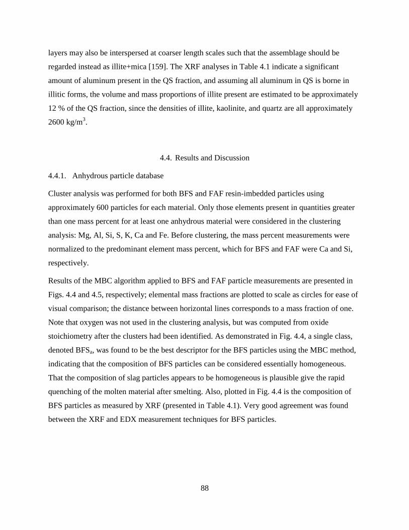
88

layers may also be interspersed at coarser length scales such that the assemblage should be

regarded instead as illite+mica [159]. The XRF analyses in Table 4.1 indicate a significant

amount of aluminum present in the QS fraction, and assuming all aluminum in QS is borne in

illitic forms, the volume and mass proportions of illite present are estimated to be approximately

12 % of the QS fraction, since the densities of illite, kaolinite, and quartz are all approximately

2600 kg/m3.

4.4. Results and Discussion

4.4.1. Anhydrous particle database

Cluster analysis was performed for both BFS and FAF resin-imbedded particles using

approximately 600 particles for each material. Only those elements present in quantities greater

than one mass percent for at least one anhydrous material were considered in the clustering

analysis: Mg, Al, Si, S, K, Ca and Fe. Before clustering, the mass percent measurements were

normalized to the predominant element mass percent, which for BFS and FAF were Ca and Si,

respectively.

Results of the MBC algorithm applied to BFS and FAF particle measurements are presented in

Figs. 4.4 and 4.5, respectively; elemental mass fractions are plotted to scale as circles for ease of

visual comparison; the distance between horizontal lines corresponds to a mass fraction of one.

Note that oxygen was not used in the clustering analysis, but was computed from oxide

stoichiometry after the clusters had been identified. As demonstrated in Fig. 4.4, a single class,

denoted BFSa, was found to be the best descriptor for the BFS particles using the MBC method,

indicating that the composition of BFS particles can be considered essentially homogeneous.

That the composition of slag particles appears to be homogeneous is plausible give the rapid

quenching of the molten material after smelting. Also, plotted in Fig. 4.4 is the composition of

BFS particles as measured by XRF (presented in Table 4.1). Very good agreement was found

between the XRF and EDX measurement techniques for BFS particles.

89

Figure 4.4: Diagram of mass fractions of BFS composition measured via XRF (BFS, presented in Table 4.1), and the centroid composition (BFSa) as calculated by the MBC method applied to measured EDX compositions. The radius of each circle is scaled according to the mass fraction of each element, and the distance between horizontal lines corresponds to a mass fraction of one.

The class representation of FAF particles derived from the MBC algorithm are presented in Fig.

4.5. The FAF material is characterized by three basic types, distinguishable primarily by their

content of Fe, with FAFc most closely matching the the mean FAF composition.

Figure 4.5: Diagram of the mass fractions of the bulk FAF composition (FAF), and the FAF subtypes (FAFa,b,c) identified using the MBC method. The radius of each circle is scaled according to the mass fraction of each element, and the distance between horizontal lines corresponds to a mass fraction of one.

90

Figure 4.6: BSE micrograph of QS quartz sand aggregate with lath-shaped phyllosilicates.

Fig. 4.6 shows a BSE micrograph of the QS used in this study mounted in resin. The large

particles in Fig. 4.6 are quartz particles, whereas the lath-shaped particles are thought to be illite

and kaolinite. Based upon the illite unit cell [159], the empirical stoichiometry of the illite in this

study observed from EDX analysis was estimated to be

(K0.67Na0.21)(Mg0.10Al2.44Fe0.05)(Si3.40Al0.60)O10(OH)2. This illite composition is quite similar to

the FAFb class of particles, which is not a surprising result given that kaolinite and illite are two

of the eight most abundant minerals found in U.S. coals [160]. These particles, however, are quite

distinct from fly ash in their geometric eccentricity. The histogram of measured eccentricities of

75 phyllosilicate particles is plotted in Fig. 4.7.

The final phase included in the anhydrous particle database is mullite, an orthorhombic and

relatively insoluble aluminosilicate found within fly ashes [161].

91

Figure 4.7: Measured distributions of particle eccentricities of the kaolinite and illite particles measured in the QS material.

Figure 4.8: Diagram of the mass fractions of the anhydrous particle database used for particle classification. The radius of each circle is scaled to the mass fraction of the constituent in that column, and the distance between horizontal lines corresponds to a mass fraction of 1. The values of the cement clinker materials (C3Styp, C2Styp, C3Atyp, C4AFtyp) were not measured herein but instead correspond to typical values [162].

The entire anhydrous particle database is illustrated in Fig. 4.8 and numerical values are provided

in Appendix E. The elements shown in Fig. 4.8 are a subset of the entire elemental composition;

due to the curse of dimensionality, including those elements that only vary slightly across all

92

compositions renders classification more difficult. Oxygen was also not considered in particle

classification due to the low accuracy of quantifying light elements.

4.4.2. Database cross-validation

To test the efficacy of the algorithm, LDA particle classification of was performed on both the

unreacted BFS and FAF particles mounted in resin. Results of this classification for BFS are

presented in Figs. 4.9 and 4.10, respectively. As shown in Fig. 4.9, LDA classification correctly

identified approximately 97% of the BFS particles. Fig. 4.10 illustrates that the correct

identification of BFS particles depends greatly on the particle size. This result is logical given

that the estimation of a particle’s mean composition improves with more samples of that

composition. As shown in Fig. 4.9, a number of small particles are simply classified as none,

which implies that these particles were, in fact, only one pixel in area so that a covariance matrix

of their composition could not be constructed, and thus, the LDA algorithms was not applied to

them. These particles account for the large number of misclassified particles with small area in

Fig. 4.10.

93

Figure 4.9: Results of the LDA classification algorithm applied to BFS particles mounted in resin. a) The original BSE micrograph of BFS particles, which appear white in the monograph. b) The BSE monograph overlain with each particle mapped with a unique color corresponding to the anhydrous database phases given in c. c) Bar graph illustrating the areas of each particle class identified. Those particles labeled “None” were not identified due to possessing too few particles to estimate the covariance matrix.

94

Figure 4.10: Area dependence of the LDA particle classification algorithm illustrated for BFS particles mounted in methacrylate resin. Particles are binned according to the base-10 logarithm of their area [pixels]. “Pct. Correct Area” indicates the area of particles correctly identified within a given bin per total area of particles within that bin. “Pct. Total Area” corresponds to the area contribution of all particles within a bin to the total area of the anhydrous BFS phase.

In Fig. 4.11, the results of the LDA algorithm applied to FAF are presented. The majority of

particles identified are fly ash particles of type FAFc, with minor amounts of the higher Fe-

content FAFa and FAFb subtypes identified. The algorithm also identifies a number of fly ash

particles as quartz, illite, and kaolinite; quartz, along with mullite, is a refractory phase found in

X-ray diffraction analyses [161]. As mentioned above, illite and kaolinite are two of the eight

most abundant mineral phases found in U.S. coals [160], but these minerals are likely melted in

the coal combustion process. Thus, the FAF particles are misidentified; however, these particles

are quite dissimilar to fly ash in their appearance. To combat such misidentification, equivalent

diameter and eccentricity have been included as auxiliary variables in the LDA analysis.

Equivalent particle diameter is defined as the diameter of an ellipsoid with an equivalent first

moment as a given region, and eccentricity is the ratio of the distance between foci of the ellipse

to the length of its major axis. Using this strategy, LDA is first executed based on elemental

composition alone; then, all particles identified as kaolinite, illite, and ash are reclassified

considering elemental composition, eccentricity, and diameter. Although a seemingly high

number of small particles are falsely identified as quartz, the quartz particles were not considered

95

in the geometric reclassification because, due to the sampling strategy, the quartz particles are

almost always truncated at the boundary of the field of view, leading to unrealistic estimates of

their particle size and eccentricities. The choice was made to misclassify a few small particles as

quartz rather than to misclassify the large quartz particles.

Figure 4.11: Results of the LDA classification algorithm applied to FAF particles mounted in resin. a) The original BSE micrograph of FAF particles, which appear white in the monograph. b) The BSE monograph overlain with each particle mapped with a unique color corresponding to the anhydrous database phases given in c. c) Bar graph illustrating the areas of each particle class identified. Those particles labeled “None” were not identified due to possessing too few particles to estimate the covariance matrix.

96

4.4.3. Estimation of reacted fractions

The results of the LDA algorithm applied to a random field of view in SVC are presented in Fig.

4.12. The original BSE intensity monograph is presented in Fig. 4.12a, and a phase map

indicating the identified phases is presented in Fig. 4.12b. The coloring of phases in Fig. 4.12b

corresponds to the bar chart in Fig. 4.12c, which shows the distribution of identified particles in

the anhydrous phase. Thus, Fig. 4.12c serves as a legend for Fig. 4.12b. It is apparent in Fig.

4.12b that, although the large quartz grains from the QS fraction (top of image) are properly

identified, a number of fly ash grains are also identified as quartz.

Figure 4.12: a) BSE monograph of an SVC field of view. b) Map of classified particles in the “anhydrous” image segment overlain on the grayscale monograph. Colors of the bars in c correspond to the coloring in b. c) Fractions of the anhydrous phase assigned to distinct classes in the anhydrous particle database.

97

Fig. 4.13 demonstrates the LDA algorithm without geometric descriptors applied to a field of

view of SVC that contains a large kaolinite particle in the northwest quadrant and a large central

illite particle that has been identified as FAFb. Fig. 4.14 shows the same field of view evaluated

with the LDA algorithm including the particle area and eccentricity descriptors. In Fig. 4.13, the

central illite particle is correctly identified, but two clustered FAF particles in the northeast

quadrant are now misidentified, likely as an artefact of their combined eccentricity. Such

misclassifications are inevitable given the similarity in phyllosilicate and fly ash compositions;

however, the differences in predicted unreacted fractions provide an indicator of the inherent

uncertainty of the method. Comparison of Figs. 4.13c and 4.14c reveal that the measured

fractions of the anhydrous phase are relatively stable for a number of species. However, the

fraction of unreacted BFS varies by approximately 34%, whereas the unreacted fraction of FAF

varies by approximately 42%, which is due to the renormalization of measured phase fractions to

the non-quartz /illite/kaolinite regions of the field of view. Thus, the error in measuring

quartz/illite/kaolinite is propagated through to the calculation of unreacted fraction. This error

could be avoided by using a completely unbiased location sampling strategy, but a high time cost

(see Section 4.2.2).

Further refinements could be made possible using expert supervision to reclassify apparently

mislabeled particles with the added cost of possible human biasing. Such a strategy would likely

require far less time to execute than manual identification of phases from scratch. In some

situations, the LDA algorithm yields visually satisfactory results, as in Fig. 4.13. LDA lends

itself to incorporating other metrics in the classification step, for instance crystallographic

information, without the need for arbitrary scaling of the metrics.

In total, BSE and EDX spectra were collected at twelve SVC sites, and from these analyses, the

reacted fractions of OPC, FAF, and BFS were estimated to be 100, 37, and 83% reacted.

Complete or nearly complete reaction of OPC is feasible given the 30-month cure age of the

specimen and comparisons with estimates of alite (C3S), belite (C2S), aluminate (C3A), and

ferrite (C4AF) reacted fractions after 2 weeks of hydration obtained from an independent BSE-

EDX investigation of the same OPC [5]. The limited reaction of fly ash is similar to that of other

fly ashes reported in the literature [125]. Eighty-three percent slag reaction is also similar in

magnitude to other reported values [163].

98

Figure 4.13: a) Map of classified particles in the “anhydrous” image segment overlain on the grayscale monograph. b) Unreacted fraction of BFS and FAF. c) Distribution of phases constituting the anhydrous portion. Colors of the bars in c) correspond to the coloring in a).

99

Figure 4.14: a) Map of classified particles in the “anhydrous” image segment using the LDA algorithm with geometric descriptors. b) Unreacted fraction of BFS and FAF. c) Distribution of phases constituting the anhydrous portion. Colors of the bars in c) correspond to the coloring in a).

4.5. Conclusions

A novel method has been presented for identifying the extent of reaction of anhydrous particles

in blended cements and mortars containing SCMs using BSE-EDX analysis. Previous methods

of particle identification have successfully utilized BSE information in the identification of

anhydrous particles, but because blended cement mortars exhibit higher degrees of material

heterogeneity than most cementitious materials, a new segmentation algorithm was developed

that integrates both BSE intensity information and EDX spectral information to identify likely

regions of anhydrous particles within a field of view. Likely anhydrous regions were compared

100

to a database of representative anhydrous particle compositions using the method of linear

discriminant analysis. Results of the classification method applied to a realistic 30-month old

blended cement mortar indicate highly satisfactory results for the identification of blast furnace

slag particles. The identification of fly ash particles is complicated by the presence of quartz and

of phyllosilicate minerals within the fine aggregate fraction of the mortar that exhibit elemental

compositions very similar to those of the fly ash. To further enhance the classification procedure

of these particles, geometric descriptors of particle shape and size were also integrated into the

discriminant analysis, which demonstrated an improved ability to identify these particles. Results

of three sampling locations indicate the estimated extent of reaction of blast furnace slag to be

83% with a coefficient of variation of 0.02 and for the fly ash, 35.8% with a coefficient of

variation of 0.27. Further refinements to this identification method have been proposed, but at

present, the algorithm executes on the order of 10 minutes. Thus, the method shows promise as a

practical means of quantifying extent of reaction in realistic, aged cementitious materials.

101

CHAPTER 5

5. CHARACTERIZATION AND MODELING OF MAJOR CONSTITUENT EQUILIBRIUM

CHEMISTRY OF A BLENDED CEMENT MORTAR2

Abstract

A blended cement mortar containing Portland cement, granulated blast furnace slag, fly ash and

quartz sand was modeled using a set of solid phases known to form in hydrated OPC with the

geochemical speciation solver LeachXS/ORCHESTRA. Comparison of modeling results to the

experimentally determined pH-dependent batch leaching concentrations (USEPA Method 1313)

indicates that major constituent concentrations are described reasonably well with the Portland

cement mineral set; however, modeled and measured aluminum concentrations differ greatly.

Scanning electron microscopic analysis of the mortar reveals the presence of Al-rich

phyllosilicate minerals: kaolinite and potassic phyllosilicates similar in composition to illite and

muscovite. Whereas both phyllosilicates are present as part of the fine aggregate, the

morphology and saturation index of kaolinite suggest that some may be formed in situ. The

inclusion of kaolinite in speciation modeling provides a substantially improved description of the

release of Al and therefore, suggests that the behavior of phyllosilicate phases may be important

for predicting long-term physico-chemical behavior of such systems.

5.1. Introduction

The extensive incorporation of ground granulated iron blast furnace slag (BFS) and coal

combustion fly ash (FAF) to cementitious materials used in barriers for nuclear waste

management has heightened the need for understanding the physico-chemical behaviors of the

resulting grout and concrete systems under use conditions in the environment and over extended

time frames. Blended cements exhibit a high degree of complexity due to the variability of both

the source and the processing of the parent materials, yielding end products comprised of a

2 Published in a special issue of the European Physics Journal as part of NUCPERF 2012

102

mixture of glassy and mineral phases. Ordinary Portland cements (OPC) are also complicated

materials but are often well-described by thermodynamic equilibrium models [164]. Whereas the

stable solid phases of ordinary Portland cement (OPC) have been studied in great detail, the

chemistry fly ash and slag blended cement has received relatively less attention. Given that OPC

is generally more reactive than slag and fly ash, the mineralogy of OPC provides a logical

starting point for describing the major constituent chemistry of blended cement mortars. To this

end, the work presented here represents a preliminary investigation of the applicability of a set of

equilibrium phases developed for Portland cement to a blended cement mortar comprised of

OPC, FAF, BFS, and quartz sand (QS).

5.2. Methods

5.2.1. Material preparation

Mortar samples for chemical characterization were prepared by mixing ordinary Portland

cement, blast furnace slag, coal fly ash, water, and quartz sand in the proportions listed in Table

5.1, resulting in a water-to-binder (w/b) ratio of 0.45. The formulation is analogous to structural

vault concretes in nuclear waste management applications [1] and is referred to herein as SVC.

Total elemental composition of the binder materials for major constituents, as determined by X-

ray fluorescence spectroscopy (XRF) are given in Table 5.2.

Each SVC specimen was cast as a slab measuring 15 cm x 30 cm x 5 cm (width x length x

height), removed from its mold after 24 hours, and allowed to cure at 98 ± 2% relative humidity

and 25 ± 1 °C in a nitrogen-purged atmosphere. After 30 months of curing, the outer surfaces of

the slabs were removed to mitigate the effects of exposed and molded surfaces, and the

remaining interior portion of the slab was crushed and sifted to less than 2 mm particle size for

use in leaching experiments.

103

Table 5.1: Raw material properties of the mortar used in this study. Particle size information was determined from particle size information provided by [138].

Material Abbrev. Mass % Density [kg/L]

Mean Particle Diameter [μm]

Median Particle Diameter [μm]

Blast Furnace Slag BFS 8.03 2.89 3.87 8.12

Type F Fly Ash FAF 16.93 2.33 6.02 14.90

Type I Cement OPC 5.40 3.01 4.16 11.30

Quartz Sand QS 55.02 2.54 590.6 596.45

Water - 14.62 1.00 - -

Table 5.2: Major element composition of the binder materials as determined by XRF, in mass percent. Carbon (C) is reported as total carbon.

Binder C O Na Mg Al Si S K Ca Fe

BFS --- 38.17 0.13 6.88 3.46 17.06 0.82 0.35 23.75 0.21

FAF 1.50 45.49 0.25 0.62 15.08 24.42 0.04 2.14 0.86 4.98

OPC 2.50 31.34 0.13 0.58 2.15 7.67 1.55 0.38 41.30 2.70

5.2.2. pH-dependent leaching test

The USEPA Method 1313 [76] pH-dependent liquid-solid partitioning protocol was used to

evaluate major constituent concentrations. Forty grams of SVC were added to 400 mL of

solution comprised of deionized water plus HNO3 or KOH/NaOH for acidification or

basification, respectively. The quantities of acid and base additions were prescribed such that

nine distinct solution pH values within a tolerance of 0.5 pH units were achieved at the end of

the extraction period: 2.0, 4.0, 5.5, 7.0, 8.0, 9.0, 10.5, 12.0, and 13.0. Two replicates of each pH

position were achieved, and for the base addition, KOH and NaOH were added to distinct

replicates in order to measure the solubility of both Na+ and K+ at high pH, respectively. Solid

samples and leaching solutions were prepared in sealed high density polyethylene bottles with

minimal headspace and tumbled end-over-end for a period of 48 hours. Once tumbled, the pH

and electrical conductivity of the leachates were measured, and the leachate was vacuum filtered.

The filtered leachate was then analyzed for total cation concentrations using inductively coupled

104

plasma optical emission spectroscopy; specific methods, detection limits and quality control

procedures used during testing are available [165].

5.2.3. Geochemical modeling

LeachXS/ORCHESTRA [63] is a geochemical speciation mass transport solver that solves

equilibrium speciation via Newton-Raphson minimization of the system of equations composed

of the laws of mass action and conservation of mass, as outlined in Chapter 2. The solid phases

considered for thermodynamic equilibrium calculations are given in Table 5.3 with solubility

products from Lothenbach, et al. [70]. Additionally, the precipitation of amorphous calcium

silicate hydrate (C-S-H) was modeled using the ideal solid solution with Tobermorite-like

(C0.8SH1.3) and Jennite-like (C1.67SH2.1) end-members proposed by Kulik and Kersten [166] with

end-member solubilities determined by Lothenbach and Winnefeld [72]. Adsorption of K+ and

Na+ onto C-S-H was modeled using partition coefficients fitted to experimental data from a study

of alkali uptake onto synthetic C-S-H gel [118]. Assuming a C-S-H surface area of 10.04 m2/kg

of C-S-H [167] and a silanol site density of 4.8 mol/nm2 [168], and specifying the surface acidity

as [168]

−SiO-+H+ ⇌ −SiOH, 𝐾 = 1.59 × 1010, (5.1)

the adsorption constants for Na+ and K+ were found to be

−SiO-+Na+ ⇌ −SiONa, 𝐾 = 1.53 × 1017

−SiO-+K+ ⇌ −SiOK, 𝐾 = 1.31 × 1017 (5.2)

where 𝐾 is the equilibrium constant and −SiO- denotes the silanol site. Adsorption onto −SiO-

of the C-S-H is the only mechanism of alkali uptake considered although the alkali filling of

interlayer spaces in aluminum-substituted C-S-H proved to be a significant sink for K+ and Na+

in synthetic gels [119] as well as for Al+3 [169, 170].

105

Table 5.3: Solid phases considered in the SVC assemblage. Species sharing superscripts indicate solid solution end-members. Mineral names are given in cement chemists’ shorthand: C – CaO, A – Al2O3, S – SiO2, F – Fe2O3, s – S2O3, c, CO2, M – MgO. Amorphous phases are denoted (am) and microcrystalline phases (mcr).

Ca(OH)2 CaCO3 CaSO4∙2H2O C3AH6 C1.67SH2.1*****

Mg(OH)2 MgCO3 C4AsH12*** C3FH6 M4AH10

******

Al(OH)3(am) C4Ac0.5H12* C4FsH12

*** C2ASH8 M4FH10******

Fe(OH)3(mcr) C4Fc0.5H12* C6As3H32

**** C2FSH8 M4AcH9

SiO2 (am) C4AcH11** C6Fs3H32

**** C3AS0.8H4.4

C6Ac3H32 C4FcH12

** K2Ca(SO4)2 C0.8SH1.3*****

Reacted fractions of OPC, FAF, and BFS were estimated to be 100, 30, and 80% reacted,

respectively based on separate electron microscopy evaluations (Chapter 4, Section 4.4.3).

Complete or nearly complete reaction of OPC is feasible given the 30-month cure age of the

specimen and comparisons with estimates of alite (C3S), belite (C2S), aluminate (C3A), and

ferrite (C4AF) reacted fractions after 2 weeks of hydration obtained from an independent

scanning electron microscopy energy dispersive X-ray (SEM-EDX) investigation of the same

OPC [5]. The limited reaction of fly ash is similar to that of other fly ashes reported in the

literature. Additionally, limited surface reaction of the Fe-rich FAF particles was observed. Such

little reaction reflects the very low concentrations of alkali and alkaline species present in FAF,

as presented in Table 5.2. Eighty percent of slag reacted is similar in magnitude to other reported

values [163].

Assuming a single value for reacted fraction of a component material implies a uniform

dissolution of each component material, a situation unlikely to occur in reality. At least one study

suggests that the dissolution of slag is substantially incongruent [171]. Indeed, in experiments

conducted by the authors, when exposed to strongly acidic solution, the BFS off-gassed H2S (g)

and formed a silicate gel. Incongruent dissolution of fly ash particles is also likely given their

glassy nature; moreover, the distinct morphologies and compositions of FAF particles suggest

distinct intrinsic solubilities among the subtypes of FAF particles. Nonetheless, a uniform

reacted fraction is expected to reflect first-order effects on the extent of binder reaction.

106

5.3. Results and discussion

Modeled concentrations using the OPC solid phases listed in Table 5.3 are compared to USEPA

Method 1313 leachate concentrations (measured in duplicate) in Fig. 5.1. The resultant

equilibrium pH without the addition of acid or base was found to be approximately 12.2

In general, the trends observed in the data are well captured by the equilibrium phases listed in

Table 5.3. The modeled solubility of Ca falls (Fig. 5.1a) within an order of magnitude of the

measured values over the pH range of interest (8<pH<13). Despite good agreement between

measured and modeled Si (Fig. 5.1b) concentrations at pH 10 and pH 12, significant

discrepancies are apparent at low and high pH. Several factors may be responsible for these

differences. First, the solid solution model of C-S-H which has been developed to describe the

formation of C-S-H is assumed here to also describe the dissolution of C-S-H; however, this

assumption may not hold if the stoichiometries of C-S-H in this study are outside the range of

those for which the C-S-H model end-member solubilities were fitted. Second, silicate phases

typically exhibit slow reaction kinetics, and therefore, the experimental results may only

approximate the final equilibrium state of the system; this scenario should be more likely near

neutral pH where reaction kinetics are typically slowest. The specific adsorption of K+ and Na+

onto C-S-H also serve as indicators of the performance of the C-S-H model because the number

of silanol adsorption sites is fixed by the total mass of C-S-H present in the system. The trends in

solubilities of K+ (Fig. 5.1c) and Na+ (Fig. 5.1d) are well captured by the geochemical model (the

increasing solubility of K+ at high pH is an artefact of the KOH addition specified by Method

1313), indicating that the mass of C-S-H formed may be well approximated by this model.

Differences in measured and modeled alkali concentrations around pH 8 may reflect a limitation

of the homogeneous reacted fraction assumption, particularly for fly ash, the most alkali-rich

binder material. Nevertheless, these differences are less than an order of magnitude.

The pH-dependent solubility of Mg is described to within an order of magnitude across the pH

range of interest (Fig. 5.1e) which suggests that the hydrotalcite-type phase is the key solubility

controlling phase for this Mg in this system. Strong correlation between total S prediction and

experiment (Fig. 5.1d) was found, owing primarily to the precipitation of ettringite.

An important deficiency in the modeling results is the characterization of aluminum. As

demonstrated in Fig. 5.2a, the solubility of Al is overestimated by 2 to 3 orders of magnitude

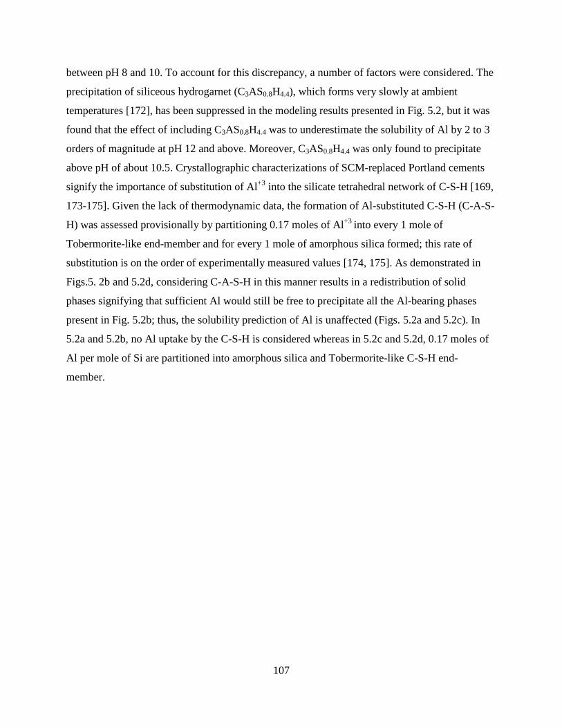
107

between pH 8 and 10. To account for this discrepancy, a number of factors were considered. The

precipitation of siliceous hydrogarnet (C3AS0.8H4.4), which forms very slowly at ambient

temperatures [172], has been suppressed in the modeling results presented in Fig. 5.2, but it was

found that the effect of including C3AS0.8H4.4 was to underestimate the solubility of Al by 2 to 3

orders of magnitude at pH 12 and above. Moreover, C3AS0.8H4.4 was only found to precipitate

above pH of about 10.5. Crystallographic characterizations of SCM-replaced Portland cements

signify the importance of substitution of Al+3 into the silicate tetrahedral network of C-S-H [169,

173-175]. Given the lack of thermodynamic data, the formation of Al-substituted C-S-H (C-A-S-

H) was assessed provisionally by partitioning 0.17 moles of Al+3 into every 1 mole of

Tobermorite-like end-member and for every 1 mole of amorphous silica formed; this rate of

substitution is on the order of experimentally measured values [174, 175]. As demonstrated in

Figs.5. 2b and 5.2d, considering C-A-S-H in this manner results in a redistribution of solid

phases signifying that sufficient Al would still be free to precipitate all the Al-bearing phases

present in Fig. 5.2b; thus, the solubility prediction of Al is unaffected (Figs. 5.2a and 5.2c). In

5.2a and 5.2b, no Al uptake by the C-S-H is considered whereas in 5.2c and 5.2d, 0.17 moles of

Al per mole of Si are partitioned into amorphous silica and Tobermorite-like C-S-H end-

member.

108

Figure 5.1: Comparison of modeled (black lines) and measured (circles and squares) major constituent leachate concentrations (as total dissolved element concentrations) of USEPA Method 1313 performed on SVC. The increasing concentration of K at high pH in c) and of Na in d) are artefacts of the leaching method: independently KOH solution and NaOH were used to adjust the pH of the leachate to a pH 12.5 ±0.5, although only the KOH addition was modeled.

109

Figure 5.2: a and c) Comparison of modeled (black lines) and measured (circles and squares) major constituent leachate concentrations and b and d). the concentrations of Al-bearing solid phases.

SEM-EDX analyses provide an indication of additional phases that may play a role in

determining Al solubility: a number of phyllosilicates (PS) are apparent within the hydrated SVC

after 30 months of curing (Fig. 5.3). To the authors’ knowledge, such phases have not been

identified previously in blends of cement, slag and fly ash, but their formation is plausible given

that PS are clay minerals that commonly form as the result of weathering, diagenesis, and low-

grade metamorphism in the natural environment. A number of PS grains are present in the

component quarts sand aggregate, but the relative abundance and wide range of sizes of these

particles in the SVC material, as well as the spatial and stoichiometric correlation of PS to fly ash

grains (Fig. 5.3), suggest that alteration of fly ash is a significant if not primary source of PS

formation. Quantitative EDX assay, an example of which is illustrated in Fig. 5.4, indicates that

these particles exhibit two basic stoichiometries: that of kaolinite (Al2Si2O5(OH)4) and that of the

mica mineral muscovite (KAl2(Si3Al)O10(OH)2). Whereas kaolinite is a common weathering

product of glassy materials such as volcanic tuff and has been shown to form in municipal solid

110

waste incinerated bottom ash [176, 177], pure muscovite typically forms in hydrothermal

environments and weathers to a class of minerals referred to as illite, a PS of the mica group

exhibiting a range of compositions somewhat intermediate between kaolinite and muscovite

[159]. In order to examine the effects of PS on the geochemical response of the SVC system, the

precipitation/dissolution reactions of kaolinite and a typical illite [178] have been considered,

although such an abstraction belies the complexity of most clay mineral systems.

Figure 5.3: BSE micrograph of kaolinite formation in close proximity to a fly ash particle in the SVC material, with an inset of the secondary electron micrograph of the FAF-PS interface.

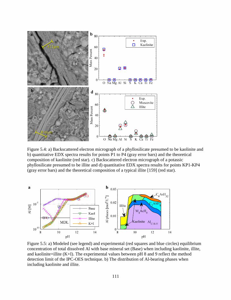
111

Figure 5.4: a) Backscattered electron micrograph of a phyllosilicate presumed to be kaolinite and b) quantitative EDX spectra results for points P1 to P4 (gray error bars) and the theoretical composition of kaolinite (red star). c) Backscattered electron micrograph of a potassic phyllosilicate presumed to be illite and d) quantitative EDX spectra results for points KP1-KP4 (gray error bars) and the theoretical composition of a typical illite [159] (red star).

Figure 5.5: a) Modeled (see legend) and experimental (red squares and blue circles) equilibrium concentration of total dissolved Al with base mineral set (Base) when including kaolinite, illite, and kaolinite+illite (K+I). The experimental values between pH 8 and 9 reflect the method detection limit of the IPC-OES technique. b) The distribution of Al-bearing phases when including kaolinite and illite.

112

Fig. 5.5a demonstrates the effects of including kaolinite and illite on the equilibrium

concentrations of Al. In general, the description of Al solubility below pH 10 is much improved,

although underestimated, by considering kaolinite in the thermodynamic equilibrium model, but

is virtually unaffected by the inclusion of illite. Including illite in the model prediction drastically

reduces the predicted solubility of K below pH 10, however, which perhaps suggests that the

illite present in SVC was present in the quartz sand parent material plays a relatively small role

in the equilibrium chemistry. That illite may be relatively unreactive in this system is further

substantiated by the observation that cracking is apparent near kaolinite grains but not illite

grains.

A few words of caution are in order concerning the inclusion of PS in thermodynamic

equilibrium models. The first is that, in the natural environment, the speciation of PS is often

complex in that PS sheets are often intermixed across multiple length scales resulting in

polymorphs, solid solutions and mixed-layer assemblages such that crystallographic

identification and chemical characterization is difficult. Second, PS undergoing dissolution and

precipitation often require months to fully equilibrate, depending on the grain size among other

factors. Whereas the mortar used in this study has been size-reduced after curing to facilitate

testing, a careful study of reaction rate would be necessary to determine if a near-equilibrium

condition has truly been reached. Examination of Fig. 5.5b reveals kaolinite is unstable above pH

of around 11.5 whereas the pore water pH of the unaltered SVC was measured as 12.2.

Estimation of saturation indices based on experimentally measured concentrations suggests that

kaolinite is supersaturated at pH 10 but undersaturated at pH 12. Therefore, from a macroscopic

thermodynamic point of view, the kaolinite observed in the SEM micrographs of SVC should be

dissolving slowly or the pH of the pore solution is somewhat less than 12 within the material.

Thus, the fact that the stoichiometry and solubility constant of kaolinite provide a more

reasonable Al response is a necessary but not sufficient condition for stating that kaolinite is

indeed the solubility-controlling mineral in this pH range for the SVC material. What can be said

is that the physical and chemical evidence strongly suggest that Al-bearing PS phases are

important for characterizing the behavior of SVC.

113

Furthermore, a rigorous characterization of the physico-chemical properties of blended cements

may require consideration of phases other than those that control solubility. For example,

considering the relatively high loading of slag in the SVC mix (52% of the binder, by mass), a

substantial portion of fibrillar magnesium silicate hydrates (M-S-H) may be expected to form

upon hydration [179], and indeed, a fibrillar product in the reaction rind of BFS is apparent in

backscattered electron micrographs, as shown in Fig. 5.6. Encapsulating the M-S-H zone is what

appears to be dense C-S-H; the presence of this sharp compositional interface suggests that

migration of constituents from the unreacted slag grain to the surrounding paste would be

controlled by the dense C-S-H layer. If M-S-H is effectively sequestered, the thermodynamic

behavior of the M-S-H may be of little consequence to the composition of the partial equilibrium

assemblage in situ; however, cracking, decalcification, and other degradation phenomena, and

especially particle size reduction, may degrade the C-S-H barrier, exposing unreacted slag to

solution and thereby altering the system equilibrium. Such a phenomenon underscores the need

for a mechanistic description of cementitious systems adaptable to a wide range of conditions.

Figure 5.6: a) Backscattered electron micrograph of a partially hydrated slag particle in unaltered SVC. b) Comparison of quantitative EDX analyses of the points H1 to H8 with the stoichiometries of sepiolite and talc, two pure phases to which synthetic M-S-H has been likened on the basis of crystallographic similarities [179].

5.4. Conclusions

A known set of Portland cement solid phases was used to model the equilibrium chemistry of a

blended cement mortar. Modeling results generally exhibited the trends and magnitudes observed

114

in a standard equilibrium pH-dependent leaching experiment, aluminum being the notable

exception. The exclusion of siliceous hydrogarnet from equilibrium calculations improved the

description of Al solubility above pH 10. Below pH 10, the description of Al solubility is greatly

improved by the inclusion of kaolinite whose presence has been inferred through SEM-EDX

analysis. The presence of potassic phyllosilicates of similar composition to illite and muscovite

was also suggested by SEM-EDX analysis; however, the inclusion of illite in thermodynamic

equilibrium model resulted in no demonstrable improvement in Al solubility prediction and a

worse prediction of K solubility. Whereas kaolinite was not definitively identified as the Al

solubility-controlling species below pH 10, the agreement between equilibrium modeling and

experiment and the SEM-EDX evidence strongly implicate Al-bearing phyllosilicates as

important species that should be considered when describing both the chemical and physical

properties of slag, fly ash and Portland cement blends.

115

CHAPTER 6

6. REACTIVE TRANSPORT MODELING OF EXTERNALLY-INDUCED AGING OF

BLENDED CEMENTITIOUS MATERIALS

Abstract

Predicting the long-term leaching behavior of blended cementitious materials requires

knowledge of the solid phases that control constituent solubility. Whereas these phases are

largely known for Portland cements, to what extent the chemical description needs to be

modified for blended cements remains an open question. Moreover, the chemical description for

long-term reactive transport prediction should encompass a number of possible phases depending

upon the chemistry of the ambient environment. An augmented set of solid phase

thermodynamic constants developed primarily for modeling the hydration of Portland cements

has been used to model the equilibrium chemistry of a blended cement mortar. Comparison of

equilibrium modeling results to both pH dependence leaching tests and to established methods of

defining the partial equilibrium assemblage indicate that the extent of reaction and the modified

set of thermodynamic parameters yield reasonable predictions of pH-dependent solubility of

major constituents. The thermodynamic model has also been applied to the modeling of aging

processes blended cement mortar monoliths, which indicate that many constituent release

behaviors seem to be described by the thermodynamic model as well. Notable exceptions and

areas for further research are highlighted.

6.1. Introduction

The widespread application of cementitious materials and the ever increasing complexity of

blended cement designs, such as those incorporating iron blast furnace slag and coal combustion

fly ash, have rendered impractical the experimental characterization of cement-based structures

over the entire range of design parameters. Moreover, cements and blended cements have been

employed extensively for the immobilization of wastes [180-182], the potency of which may be

only slowly diminished if at all. The service life of these cementitious barriers may span

116

thousands of years, making experimental characterization impossible over the time frames of

interest. For these reasons, the mechanistic description of the

The field of cement science has only very recently turned its attention to the rigorous

mineralogical characterization of cements that incorporate pozzolanic materials, that is, those

containing reactive silica. The additional complexity introduced by the incorporation of wastes

into the cementitious matrix exacerbates the need for fundamental understanding of these

materials. In the field of waste management, however, the systematic thermodynamic

characterization and modeling of cementitious waste forms is highly varied and heterogeneous

materials 1) have demonstrated the similarities in leaching behaviors of highly diverse

cementitious systems and 2) have led to the inference of a number of underlying mechanisms

controlling constituent release in both laboratory and field testing experimental scenarios [6,

183-188]. Such studies are invaluable in assessing both where uncertainties in the mechanistic

description lie and in gauging the magnitudes of those uncertainties. It is within this context that

the present work seeks to examine a blended cement mortar (denoted SVC) typical of the

structural vaults concretes used in cementitious waste barrier applications [1].

In Chapter 4, backscattered electron microscopy coupled with energy dispersive X-ray (BSE-

EDX) analysis was used to quantify the extent of reaction of the ordinary Portland cement

(OPC), Class-F coal combustion fly ash (FAF), Grade 100 blast furnace slag (BFS), and graded

quartz sand (QS) which comprised the mortar. Chapter 5 examined how well a set of equilibrium

phases developed for Portland cement [70, 164] described SVC by comparing model predictions

to standard pH-dependent batch leaching tests [76, 165, 189]; with a few additions and

modifications, it was determined that major constituent solubility as a function of pH was

generally well-described by a subset of solid phases developed for modeling the hydration of

ordinary Portland cement. The present work builds upon this idea by using standard leaching

protocols as a means of investigating the validity of the component masses calculated from

reacted fraction measurements. The first objective of this work is to vary the extent of reacted

fraction parameters over a feasible range to assess both the sensitivity and the accuracy of the

partial equilibrium representation of SVC. Results are compared to established methods of

determining component masses.

117

The second goal of the present work is to investigate the response of the thermodynamic model

to chemical aging as a result of exposure to external leaching solutions. Thus, the second primary

objective is to compare reactive transport simulations, which employ the thermodynamic

description of SVC, to measurements of constituent release and/or uptake in four distinct aging

scenarios. The four aging conditions considered herein are exposure to deionized water, sodium

sulfate, magnesium sulfate, and sodium carbonate solutions, each of which may be considered an

“accelerated” aging solution in that the differences in composition between the cement system

and the external solutions are more extreme than would normally be expected in the natural

environment.

6.2. Materials and methods

6.2.1. Component materials

The blended cement mortar studied is composed of Type I/II Portland cement OPC [134], grade

100 ground granulated blast furnace slag (BFS) [135], Type F coal combustion fly ash (FAF)

[136], and quartz sand (QS) [137]. Total elemental composition for the major constituents of all

four materials, as determined by X-ray fluorescence (XRF) spectroscopy (Arcadis, USA) are

given in Table 6.1.

Table 6.1: Major element composition of the component materials as determined by XRF, in mass percent. Carbon (C) is reported as total carbon.

Binder C O Na Mg Al Si S K Ca Ti Fe

BFS --- 38.17 0.13 6.88 3.46 17.06 0.82 0.35 23.75 .03 0.21

FAF 1.50 45.49 0.25 0.62 15.08 24.42 0.04 2.14 0.86 1.67 4.98

OPC 0.39 34.62 0.21 0.69 2.59 9.15 1.20 0.53 43.90 0.16 4.49

QS 0.93 52.35 0.02 0.00 2.45 43.82 0.00 0.18 0.01 0.02 0.21

Blended mortar samples (SVC) were prepared by mixing OPC, BFS, FAF, and QS in the

proportions listed in Table 6.2; this formulation is within the family of compositions used as

structural concretes in nuclear waste management applications, with the exception that no coarse

118

aggregate is present in the mortar presently studied [1]. SVC specimens were cast as slabs

measuring 15 cm x 30 cm x 5 cm (width x length x height), removed from their molds after 24

hours, and allowed to cure at 98 ± 2% relative humidity and 25 ± 1°C in a nitrogen-purged

atmosphere for 30 months. Samples for granular material leaching tests were generated by first

grinding and discarding the outer surfaces of a slab and then crushing and sifting the material to

a particle size of less than 2 mm.

Table 6.2: Mix design of the blended cement mortars studied herein, SVC.

Component Mass % Vol. %

BFS 8.0 5.8

FAF 16.9 15.1

OPC 5.40 6.0

QS 55.0 45.0

Water 14.6 30.4

6.2.2. pH dependent leaching

The USEPA Method 1313 [76] pH-dependent liquid-solid partitioning protocol was used to

evaluate major constituent concentrations. Forty grams of SVC were added to 400 mL of

solution comprised of deionized water and HNO3 or KOH for acidification or basification,

respectively. The quantities of acid and base additions were prescribed such that five distinct

solution pH values, within a tolerance of 0.5 pH units were achieved at the end of the extraction

period: 2.0, 4.0, 5.5, 7.0, 8.0, 9.0, 10.5, 12.0, and 13.0. The acid and base additions and resultant

pH are given in Table 6.3 for the pH range of 8 to 14 and for the lowest pH for determination of

availability as per Method 1313. The pH point at 12.0±0.5 was obtained without the addition of

acid or base and is termed the “own pH” of the material. Solid samples and leaching solutions

were prepared in sealed high density polyethylene bottles with minimal headspace and tumbled

end-over-end for a period of 48 hours. Once tumbled, the pH and electrical conductivity of the

leachates were measured, and the leachate was vacuum filtered. The filtered leachate was then

analyzed for total cation concentrations using inductively coupled plasma optical emission

119

spectroscopy. The entire extraction procedure was performed in duplicate. Specific methods,,

detection limits, and quality control procedures used during testing are available in [165].

Table 6.3: Equivalent base additions and resultant pH for the Method 1313 leach test.

Mean equivalent base addition [meq/gram] Solution pH

0.68 13.02

0.00 12.225

-0.79 10.065

-1.80 8.685

-4.2 1.69

6.2.3. Accelerated aging

After 30 months of curing, cylinders measuring 18.0 ± 0.5mm outside diameter were cored from

the slabs. The radial surface of each cylinder was ground using a progression of silicon carbide

papers in order to eliminate the annular high-porosity region created by the coring process. The

top and bottom of each cored cylinder were sawn off using a low speed saw in order to minimize

the effects of air-exposed and molded surfaces, respectively. Each cylinder was then cast into a

cylindrical acrylic sleeve with methacrylate resin, and the top of the cylinder and sleeve were

again sawn to yield a cylinder of 20 ± 0.5 mm in length with a single exposed face, establishing a

one-dimensional diffusion boundary. Sequential grinding and diamond-paste polishing of the

exposed face followed by 20 seconds of sonication in acetone was performed in order to

eliminate artificial porosity created by sawing.

Leaching of monolith cylinders was accomplished using a modified version of the draft USEPA

monolith leaching protocol [68] wherein monolithic materials are exposed to an external solution

of deionized water (DI) at a ratio of 10 L of solution per cm2 of exposed monolith surface area,

which is commonly known as the finite bath boundary condition within numerical contexts. Four

distinct leaching solutions were chosen to simulate the aging of cementitious samples in

aggressive environments: DI and aqueous solutions of 0.250 [M] Na2SO4 (NS), 0.015 [M]

MgSO4 (MS), and 0.350 [M] Na2CO3 (NC). DI leaching was selected to induce decalcification of

120

the C-S-H phase primarily and serves as a reference condition, whereas NS and MS solutions

were expected to form ettringite, hydrotalcite-like minerals, and possibly M-S-H in the case of

MgSO4 exposure. NC solution was selected as a means of forming carbonates independent of the

pH depression concomitant with gas phase carbonation. Aging solutions were refreshed at

approximately 1 week intervals, at which point the leaching solution was measured for pH and

electrical conductivity, vacuum filtered, and analyzed for cation composition using inductively

coupled plasma optical emission spectroscopy.

6.3. Reactive transport modeling

6.3.1. Geochemical equilibrium modeling

LeachXS/Orchestra (LXO) [63] is a geochemical speciation mass transport solver that solves

equilibrium speciation via Newton-Raphson minimization the system of equations comprised of

the laws of mass action and conservation of mass, as detailed in Chapter 2, Section 2.2.3.

Conservation of mass is imposed by designating a subset of all possible aqueous species as

primary species, 𝑝 and prescribing the mass of 𝑝, 𝑀𝑝 [mol] that is assumed to take part in

equilibrium chemistry assemblage. Using backscattered electron microscopy coupled with

energy dispersive X-ray analysis (Chapter 4), reacted fractions of OPC, FAF, and BFS were

estimated for the SVC mortar such that the 𝑀𝑝 of each major species may be calculated as

𝑀𝑝 = �𝛼𝑞𝜑𝑞𝑥𝑞,𝑝𝑞∈ 𝑄

(6.1)

where 𝛼𝑞 is the degree of reaction of the 𝑞𝑡ℎ reactive constituent material, 𝜑𝑞 is the mass

fraction of the 𝑞𝑡ℎ phase specified in the mix design, and 𝑥𝑞,𝑖 [mol] is total mass of the 𝑖𝑡ℎ

component of constituent 𝑞. Alternatively, 𝑀𝑝 may be obtained from the maximum solubility

concentrations measured in the Method 1313 pH-dependent leaching test [189], which are herein

referred to as “availabilities” of primary species.

Stability constants were obtained for aqueous species known to be important for geologic media

and are presented in Appendix A, as described in Chapter 2. The solid phases modeled in this

study are typical of those used in the modeling the hydration of Portland cements, and their

stability constants are provided in Table 6.4. Notably, the precipitation of calcium silicate

121

hydrate (C-S-H) was modeled using the ideal solid solution model with Tobermorite-like and

Jennite-like end-members proposed in [166]. The layered double hydroxide phases commonly

employed in hydration modeling have been omitted from the present modeling, as it was found

that the inclusion of the M4AH10 hydrotalcite-like phase, either as a pure phase or as a solid

solution end-member, resulted in the underestimation of Mg solubility by two orders of

magnitude near the own pH of the material. Brucite, however, was found to yield a very close

prediction of Mg solubility. As described in Chapter 5, kaolinite is a solid phase not normally

found in Portland cements, but its inclusion in the partial equilibrium assemblage led to an

improved pH-dependent description of Al solubility, particularly at low pH. Also described in

Chapter 5 is that the uptake of Al into C-S-H (C-A-S-H) is likely an important factor for

describing the blended SVC chemistry. Do to the lack of thermodynamic stability parameters for

C-A-S-H, the partial equilibrium mass of Al was, therefore, heuristically adjusted prior to each

equilibrium calculation; eighty percent of every mole of Si is assumed to form C-S-H, and 0.17

moles of Al per mole of C-S-H are assumed to form C-A-S-H. Therefore, the Al content in

partial equilibrium is that specified either by reacted fractions or availabilities less 0.136 moles

of Al per mole of Si specified.

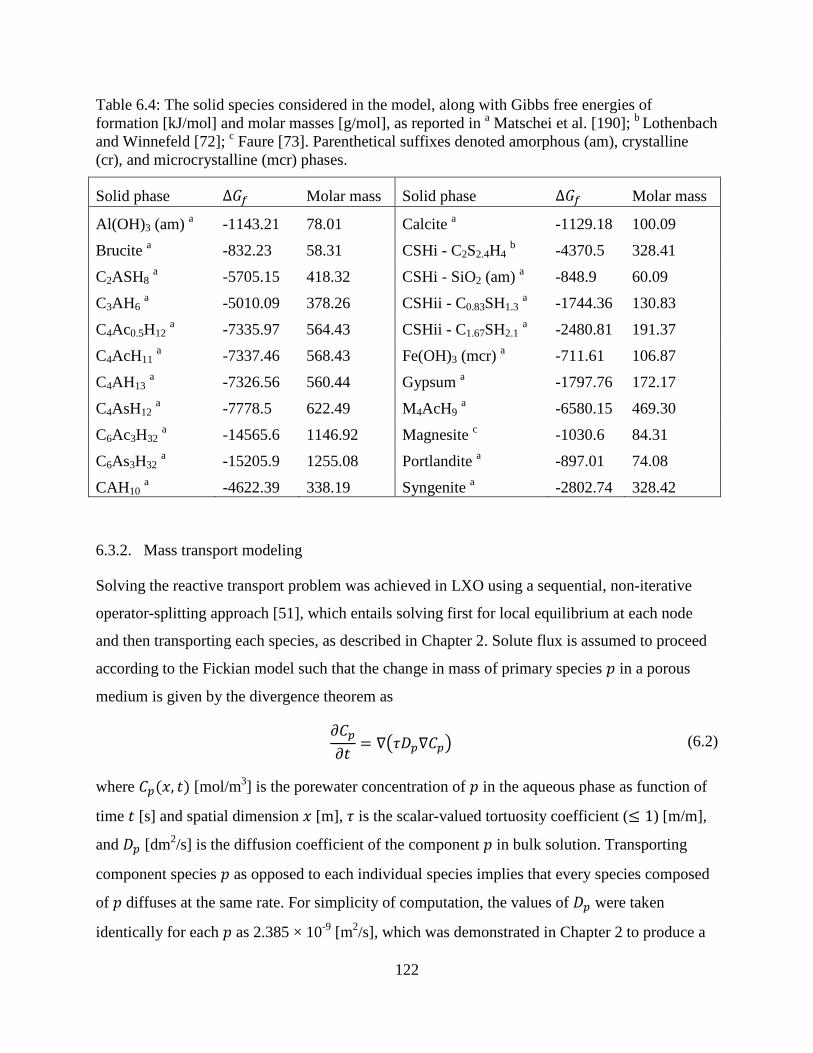
122

Table 6.4: The solid species considered in the model, along with Gibbs free energies of formation [kJ/mol] and molar masses [g/mol], as reported in a Matschei et al. [190]; b Lothenbach and Winnefeld [72]; c Faure [73]. Parenthetical suffixes denoted amorphous (am), crystalline (cr), and microcrystalline (mcr) phases.

Solid phase Δ𝐺𝑓 Molar mass Solid phase Δ𝐺𝑓 Molar mass

Al(OH)3 (am) a -1143.21 78.01 Calcite a -1129.18 100.09

Brucite a -832.23 58.31 CSHi - C2S2.4H4 b -4370.5 328.41

C2ASH8 a -5705.15 418.32 CSHi - SiO2 (am) a -848.9 60.09

C3AH6 a -5010.09 378.26 CSHii - C0.83SH1.3 a -1744.36 130.83

C4Ac0.5H12 a -7335.97 564.43 CSHii - C1.67SH2.1 a -2480.81 191.37

C4AcH11 a -7337.46 568.43 Fe(OH)3 (mcr) a -711.61 106.87

C4AH13 a -7326.56 560.44 Gypsum a -1797.76 172.17

C4AsH12 a -7778.5 622.49 M4AcH9 a -6580.15 469.30

C6Ac3H32 a -14565.6 1146.92 Magnesite c -1030.6 84.31

C6As3H32 a -15205.9 1255.08 Portlandite a -897.01 74.08

CAH10 a -4622.39 338.19 Syngenite a -2802.74 328.42

6.3.2. Mass transport modeling

Solving the reactive transport problem was achieved in LXO using a sequential, non-iterative

operator-splitting approach [51], which entails solving first for local equilibrium at each node

and then transporting each species, as described in Chapter 2. Solute flux is assumed to proceed

according to the Fickian model such that the change in mass of primary species 𝑝 in a porous

medium is given by the divergence theorem as

𝜕𝐶𝑝𝜕𝑡

= ∇�𝜏𝐷𝑝∇𝐶𝑝� (6.2)

where 𝐶𝑝(𝑥, 𝑡) [mol/m3] is the porewater concentration of 𝑝 in the aqueous phase as function of

time 𝑡 [s] and spatial dimension 𝑥 [m], 𝜏 is the scalar-valued tortuosity coefficient (≤ 1) [m/m],

and 𝐷𝑝 [dm2/s] is the diffusion coefficient of the component 𝑝 in bulk solution. Transporting

component species 𝑝 as opposed to each individual species implies that every species composed

of 𝑝 diffuses at the same rate. For simplicity of computation, the values of 𝐷𝑝 were taken

identically for each 𝑝 as 2.385 × 10-9 [m2/s], which was demonstrated in Chapter 2 to produce a

123

response near the mean rate of migration predicted the Nernst-Planck transport model for

solutions typical of cement porewaters.

For the 1-D diffusion regime dictated by the sample geometry, the boundary condition on the

right is specified by the zero-flux condition:

𝜏𝐷𝑝𝜕𝐶𝑝𝜕𝑥

= 0 , 𝑥 = 𝑎, 𝑡 > 0 (6.3)

where 𝑎 is the length of the specimen [m]. On the left, the finite bath condition is given by

𝑉𝑡𝑎𝑛𝑘𝜕𝐶𝑝𝜕𝑡

= 𝜏𝐴𝑠𝑢𝑟𝑓𝐷𝑝𝜕𝐶𝑝𝜕𝑥

, 𝑥 = 0, 𝑡 > 0 (6.4)

where 𝑉𝑡𝑎𝑛𝑘 is the volume of the external solution or tank [m3], 𝐴𝑠𝑢𝑟𝑓 is the surface area of the

specimen [m2], and 𝑥 = 0 specifies the location of the solution-specimen interface. Due to the

well-mixed assumption, the concentration 𝑝 at 𝑥 = 0 is both the concentration at the surface of

the porous medium and the concentration of the tank. The solid domain, that is 0 ≤ 𝑥 ≤ 𝑎, was

divided into 21 nodes using a geometrically increasing node spacing with a 0.75 mm minimum

node spacing in order to meet the requirements of the local equilibrium assumption [48]. The

simulation timestep was set to a value of 100 s for the first three hours after refresh of the tank

solution in order to improve accuracy of the FD scheme; otherwise, a constant timestep of three

hours was used.

6.4. Results

6.4.1. Reacted fractions and availabilities

As described in Chapter 4, the reacted fractions of OPC, FAF, and BFS were determined to be

100%, 36%, and 83% reacted, respectively, using BSE-EDX analysis. The values of input

primary species masses for equilibrium modeling, 𝑀𝑝, determined through Eq. (6.1) are given in

Table 6.5. Also shown in Table 6.5 are the availabilities of primary species as determined by the

maximum soluble concentrations measured in the Method 1313 leaching protocol [2].

124

Table 6.5: Masses of the primary species, 𝑀𝑖, used as input for equilibrium modeling, expressed in units of moles per kg of dry solid.

Component Reacted Fraction Availability

CO3 0.0387 0.0022

Na 0.0147 0.0073

Mg 0.2502 0.2480

Al 0.3629 0.2229

Si 1.028 0.5755

SO4 0.0622 0.0243 Cl 1.454(10-3) 3.393(10-4)

K 0.0428 0.0368

Ca 1.120 0.9003

Fe 0.0869 0.0257

Ca/Si 1.09 1.56

Al/Si 0.36 0.39

Figure 6.1: Graphical representation of the molar proportions of major primary species participating in the partial equilibrium assemblage as predicted by the availability from Method 1313 (“1313”) and from the sum of reacted fractions as measured in Chapter 4.

Fig. 6.1 illustrates the proportions of Mg, Al, Si, and Ca measured by the two techniques relative

to one another. The 𝑀𝑝 are quite similar for the shown primary speciess; the Method 1313

availabilities indicate higher amounts of Mg and Ca in the partial equilibrium assemblage than

those determined via BSE-EDX analysis which may reflect an incongruent reaction of FAF and

BFS particles given that Al and Si may be kinetically controlled in certain media.

125

The sensitivity of primary species’ solubilities to 𝑀𝑝 is difficult to gauge a priori because the

predicted solubilities will only change when the stable mineral assemblage changes, that is, when

a different stoichiometric reactant becomes limiting for at least one solid phase. Therefore, the

chemical response of the system as a function of varying extent of reaction is discussed next.

6.4.2. Geochemical equilibrium modeling

To address the uncertainties in the measurements of reacted fraction in Chapter 4 and to

understand better the behavior of the thermodynamic model, the parameters 𝛼𝐵𝐹𝑆 and 𝛼𝐹𝐴𝐹 were

varied over the intervals [0.6,1.0] and [0.0,0.8], respectively, using a Latin hypercube sampling

(LHS) design of experiments [139]. A total of 100 model runs were computed with varied 𝛼𝑞,

and modeling outputs were compared to the results of the Method 1313 pH-dependent leaching

test at four equivalent base additions of -1.8 [meq/gram] to 0.68 [meq/gram] corresponding to pH

points spanning the range of pH 8.7 to 13.0 as listed in Table 6.3. Shown in Fig. 6.2a is the pH

response as a function of acid or base addition with continuous simulation between the

experimental points at which the residual was calculated. The curve in Fig. 6.2a labeled “RF”

corresponds to the thermodynamic response calculated with reacted fractions of 𝛼𝐹𝐴𝐹 = 0.20

and 𝛼𝐵𝐹𝑆 = 0.83 whereas the curve label “1313” shows the same calculation performed using

primary species masses calculated using availabilities from Method 1313. Shown in Fig. 6.2b is

a contour plot of the mean error computed at all 100 sample points. Unsurprisingly, the pH

response is much more sensitive to the reacted fraction of FAF than BFS because FAF

constitutes more than twice the total mass of BFS specified in the mix design. The rectangular

region highlighted in Fig. 6.2b is centered on the mean values of 𝛼𝐵𝐹𝑆 and 𝛼𝐹𝐴𝐹 and spans one

standard deviation to either side of the mean. The band of minimum pH residuals situated at

approximately on 𝛼𝐹𝐴𝐹 = [0.01,0.22] is encompassed this “uncertainty region” although it is

relatively far from the mean measured value of 𝛼𝐹𝐴𝐹. Additionally, annotated on the intensity

scale of Fig. 6.2b is the mean error computed when using 𝑀𝑖 computed from Method 1313 in

lieu of reacted fraction quantities and the same thermodynamic parameters.

126

Figure 6.2: a) The response of system pH in both simulation (blue and green lines) and experiment (gray boxes) as a function of milliequivalents of base added per gram of solid material. “1313” denotes the simulation wherein 𝑀𝑖 was determined through Method 1313 availability measurement and “RF” denotes the determination of 𝑀𝑖 through the reacted fraction BSE-EDX analysis. b) Contour plot of the mean error in pH computed from comparison of model responses to pH-dependent batch leaching as a function of varied reacted fractions. The magnenta rectangle is centered on the measured values of 𝛼𝐵𝐹𝑆 and 𝛼𝐹𝐴𝐹 and spans two standard deviations in those measurements, as determined in Chapter 4. The text label “1313” indicates the mean error predicted when the availabilities measured from Method 1313 are used in lieu of the reacted fraction quantities. The yellow star indicates the reacted fractions of 𝛼𝐵𝐹𝑆 = 0.83 and 𝛼𝐹𝐴𝐹 = 0.20 used for calculation of pH in a).

Presented in Fig. 6.3 are the mean errors computed for the primary species Ca, Si, Mg, and Al.

Errors have been calculated in base 10 logarithms in order to scale relative solubilities to a more

comparable range. Thus, a mean error of one corresponds to an order of magnitude difference in

prediction and experiment. Similar to pH, the mean errors of Ca, Si, Mg, and Al are highly

correlated to 𝛼𝐹𝐴𝐹 . Interestingly, the minima for the primary species present in Fig. 6.3 do not

necessarily coincide with the minima for pH. The region of minima for Ca (Fig. 6.3a) are banded

at a slightly higher value of 𝛼𝐹𝐴𝐹 than was pH, whereas the Mg minima are nearly coincident

with the minima for pH, a correlation that is likely a result of the sensitivity of Mg solubility to

pH. The responses of Al and Si are also highly correlated with the exception that the region of

minima for Al is bounded for low values of 𝛼𝐹𝐴𝐹 whereas Si is not.

Figs. 6.4a and 6.4b illustrates the contour plots of Na and K errors, respectively. Both primary

species tend to decrease with decreasing 𝛼𝐹𝐴𝐹, primarily, although the concentrations of Na

127

depend upon 𝛼𝐵𝐹𝑆 as well. Because no solid phase reactions are specified for Na and K, the

trends in Fig. 6.4 are a direct reflection the extent of reaction. Also shown in Fig. 6.4 are the

measured availabilities of Na and K; since the availabilities are generally lower than the reacted

fraction amounts, the mean error observed using available concentrations is generally lower,

which suggests an omitted mechanism of alkali uptake in the thermodynamic description.

Figure 6.3: Contour plots of the mean errors in major primary species computed from comparison of model responses to pH-dependent batch leaching. The magenta rectangle delineates the BSE-EDX measurements of 𝛼𝐵𝐹𝑆 and 𝛼𝐹𝐴𝐹 ± one standard deviation, as measured in Chapter 4. The arrow labeled “1313” corresponds to the error computed by defining component masses with availabilities measured via Method 1313.

128

Figure 6.4: Contour plots of the mean errors in alkali primary species computed from comparison of model responses to pH-dependent batch leaching. The magenta rectangle delineates the BSE-EDX measurements of 𝛼𝐵𝐹𝑆 and 𝛼𝐹𝐴𝐹 ± one standard deviation, as measured in Chapter 4. The arrow labeled “1313” corresponds to the error computed by defining component masses with availabilities measured via Method 1313.

Examination of Figs. 6.2-6.4 indicates that the region near 𝛼𝐵𝐹𝑆 = 0.83 and 𝛼𝐹𝐴𝐹 = 0.20

contains near-minimal values for the considered primary species and also lies within the

uncertainty region of measured reacted fractions. Therefore, the composition of 𝛼𝐵𝐹𝑆 = 0.83 and

𝛼𝐹𝐴𝐹 = 0.20 was chosen as a reasonable approximation of the mass of the partial equilibrium

assemblage for subsequent mass transport modeling.

The results of pH-dependent modeling and experiment for Ca, Si, Mg, and Al are depicted in

Fig. 6.5. Also shown are the results of the pH dependence test using available 𝑀𝑖 measured in

Method 1313. The general trends between the two methods of determining 𝑀𝑖 are very much the

same; the simulation of Mg is nearly identical between the two methods, and the predictions are

within an order of magnitude of the experimental values. Al and Si are better predicted with

availabilities above pH of approximately 11, and in the case of Al, the difference is nearly an

order of magnitude. This result may be indicative of over-estimation of the reacted fractions in

Chapter 4 in conjunction with an incongruent reaction of the FAF and BFS materials. The

reacted fraction prediction of Ca solubility lies closer to the measured values, and the reason for

this may be the higher Ca/Si ratio for the availability measurements.

129

Figure 6.5: Experimentally measured values (gray squares) of component solubility from the Method 1313 leaching protocol and geochemical equilibrium modeling results using both availabilities (“1313”) and reacted fractions (“RF”).

Overall, neither model attains the full range of measured pH values as a result of acid and base

addition, but the agreement between model and prediction is fairly good in the vicinity of the

own pH of SVC. It is anticipated that the development of a C-A-S-H solid solution model may

greatly improve the description of both Al and Si, as the ad hoc approach to mimic C-A-S-H

stoichiometry resulted in improved model predictions.

130

6.4.3. Tortuosity determination

Tortuosity is a necessary parameter for modeling diffusive transport (Eq. 6.2) but, unfortunately,

is not directly measurable. A non-reacting species could be used to calibrate the tortuosity to

experimental data, but in cementitious materials, even species with characteristically high

solubilities may interact with the solid material. Such behavior is suspected in the case for

alkalis, which are known to be adsorbed by and substituted in synthetically prepared C-S-H

[118] and C-A-S-H [119, 191]. Recently, Chappex and Scrivener [192] reported no significant

influence of alumina substitution on the uptake of alkali in “real blended pastes”; however, their

study focused on silica fume and metakaolin blends with Ca/Si ratios of the C-S-H in the range

of 1.5. In a seminal work by Hong and Glasser [119], the alumina incorporated into C-S-H with

Ca/Si of 1.5 was found to have little impact on the sorptive capacity of synthetic gels. Chappex

and Scrivener cited this result as evidence of that Al incorporation into C-S-H does not

substantially lower the alkalinity of pore waters. However, in the same study by Hong and

Glasser, it was found that for gels with Ca/Si of 0.85, the C-A-S-H uptake of alkalis was an order

of magnitude higher than that of the equivalent C-S-H paste. Codina et al. [193] found that in 12

month old blended pastes with Ca/Si ratios near 1.0, the alkali concentrations in expressed pore

solution were on the order of 10-3 M as compared to approximately 0.1 M for a PC paste with

comparable initial alkali content. Moreover, the decrease in porewater alkalinity was found to

decrease with curing time. In the present study, the calculated Ca/Si of the C-S-H is

approximately 0.86, which is very close to the lowest synthetic gel studied by Hong and Glasser.

The replacement levels of OPC with slag and fly ash are also similar to those of the study in

[193]. Therefore, it seems possible that in the 30-month aged SVC material, a significant level of

alkali binding occurs. Furthermore, the possibility of alkali uptake in clay minerals cannot be

completely ruled out given the findings in Chapter 5.

Because no mechanisms for alkali adsorption have been considered in the present geochemical

model and no alkali-bearing minerals are predicted to be stable in the unperturbed material, the

entirety of the Na and K primary species are present as dissolved species. Therefore, to find

parameter values which describe the release of Na and K, a Latin hypercube sampling (LHS)

scheme was carried out in order to efficiently vary across the parameter space both tortuosity and

Na and K input component concentrations, Na0 and K0 [M], respectively,. Alkali concentrations

131

were varied from 0.1% to 110% of their estimated values from the SEM-EDX analysis of

Chapter 4, a range which also encompasses their measured availability from Method 1313. Using

LHS, 500 sample points were chosen, which for a 3-dimensional problem conforms to the rule of

thumb for LHS that the number of points should be ten times greater than the number of

dimensions [194]. Mean squared error (MSE) residuals were computed by comparing the base 10

logarithms of simulated concentrations to the experimentally measured concentrations for the DI

water monolith leaching case.

Figure 6.6: Mean squared errors computed from comparison of simulation and experimental data for the DI leaching case. Shown are a) Na MSE as function of initial Na and tortuosity, b) K MSE as a function of initial K and tortuosity. Magenta pentagrams indicated the 20 lowest residuals computed for each ion.

As shown in Fig. 6.6, a diagonal band of minima is apparent for linear combinations of 𝜏 and

initial concentration variations. As a simplification, it is assumed in this work that the adsorption

isotherm reported in [119] may be represented as

𝑆𝑖 = 𝑅𝐶𝑖 + 𝑏 (6.5)

where 𝑆𝑖 [molads/Lsol] is the sorbed portion of constituent 𝑖, 𝑅 is the retardation factor [-], and 𝑏 is

a fitting parameter [molads/Lsol]. Eq. (6.5) implicitly assumes that the adsorption isotherm is

independent of the liquid-to-solid ratio of the system, and the retardation, and the retardation

factors calculated in this manner range between approximately 0.4 and 2.5 for both alkalis. These

132

values of 𝑅 seem insufficient per se to explain a reduction in porewater alkalinity by two orders

of magnitude found in [193]. It is, therefore, concluded, that more fundamental research is

needed for describing alkali uptake. Whereas an isotherm could be constructed to fit model alkali

uptake in the present material, based upon the results in Fig. 6.6 it seems likely that a semi-

infinite number of isotherms parameters may be yield approximately the same response.

Therefore, two limit cases are chosen for examination: 𝜏 = 500 and 𝜏 = 60,000. The first

proposed value of tortuosity corresponds to a reasonable estimate of the lower limit given that

the SVC material had aged for 30 months at the time of testing and it is generally accepted that

the addition of pozzolanic materials leads to porosity refinement. The second value corresponds

to the tortuosity value assuming all of the alkalis are present in dissolved form. In both cases, a

value of initial alkali was roughly fit to the system response. As demonstrated in Fig. 6.7, a

slightly better prediction of the alkali release in the DI water case could be achieved using a

lower tortuosity value. However, as shown in Fig. 6. 8, the release of precipitating primary

species is largely insensitive to the value of tortuosity. Moreover, the pH of the tank solution

(Fig. 6.9) is relatively unchanged by the value of tortuosity, as well. This observation is not

intended to negate the importance of tortuosity in describing the physical evolution of

cementitious materials nor does it discount the relative impact of tortuosity in long time frames,

but for the purposes of the materials and time frames considered in this study, the value of

tortuosity exerts little influence on the overall predictions. Porosity and tortuosity changes

induced by mineralogical changes are also like to play a role, but for the remainder of this work,

a constant value of 𝜏 = 500 has been prescribed.

133

Figure 6.7: Comparison of modeled (blue “+” and green “x”) and experimentally measured (gray squares) tank concentrations of alkali ions in the DI water leaching scenario using values of 𝜏 = 500 (blue “+” signs) and 𝜏 = 60,000 (green “x”). Lines connecting data points do not represent interim concentration values; they are simply present to guide the eye.

134

Figure 6.8: Comparison of modeled (blue “+” and green “x”) and experimentally measured (gray squares) tank concentrations of major ions in the DI water leaching scenario using values of 𝜏 = 500 (blue “+”) and 𝜏 = 60,000 (green “x”). Lines connecting data points do not represent interim concentration values; they are simply present to guide the eye.

135

Figure 6.9: Comparison of modeled (blue “+” and green “x”) and experimentally measured (gray squares) tank pH in the DI water leaching scenario using values of 𝜏 = 500 (blue “+”) and 𝜏 = 60,000 (green “x”). Lines connecting data points do not represent interim concentration values; they are simply present to guide the eye.

6.4.4. SVC leaching

Results of the four accelerated aging cases outlined in Section 2.3 are presented together in this

section in order to facilitate comparisons between them. Because no explicit mechanism for

alkali adsorption was modeled, the predicted releases of K are essentially the same for all four

scenarios. In Fig. 6.10, however, it is apparent that the measured release of K is roughly an order

of magnitude lower in the DI leaching scenario than in the other three; a possible explanation is

that K+ bound within the C-S-H phases is displaced by the intruding cations. Such behavior is

expected from intruding Na+ ions which may participate in adsorption and cation exchange

reactions in a manner similar to K+. On the contrary, the divalent Mg+2 ion is unlikely to

substitute for K+, yet the releases of Na and K are higher in the MS leaching case than in the DI

case. The formation of magnesium silicates, namely magnesium-silicate-hydrate (M-S-H) [179,

195], may explain this higher alkali release, as it is conceivable that the reconfiguration of silica

into magnesium silicates liberates alkalis from the gel phase.

136

Figure 6.10: Experimentally measured (open symbols) tank concentrations of a) Na and b) K as a function of the square root of leaching time for the four leaching cases.

Further suggestion of the presence of M-S-H in the MS case is apparent in the release of Si (Fig.

6.11b); for the cases of DI, NC, and NS leaching (Fig. 6.11), the prediction of Si release matches

the data fairly closely, which may be taken as an indication that the CSHii solid solution model is

reasonable for describing Si release in a system that almost assuredly contains Al-substituted C-

S-H [173-175, 196, 197]. In the MS case, however, the Si release is overpredicted by

approximately 3 orders of magnitude and diverges from the experimental trend. One possible

explanation is that Si solubility is being suppressed by an M-S-H phase; an alternative is that the

formation hydrotalcite-like phases and ettringite tend to remove Al from the C-A-S-H structure,

leading to stronger affinity for Si in the gel phase.

As shown in Fig. 6.12, Al release is overestimated for the DI and NS cases by generally less than

an order of magnitude, a difference which may attributable to the lack of a thermodynamic

description of C-A-S-H. Examination of the Al release in Fig. 6.12b and the Mg uptake in Fig.

6.13b for the MS case suggest that the hydrotalcite-like phases (M4AH10) [198, 199] should be

stable under these conditions. As discussed in Section 3.1, the hydrotalcite-like phases have been

omitted from consideration due to their poor description of the equilibrium solubility of Mg. This

discrepancy may be due in part to the fact that the stability constants ascribed to the hydrotalcite-

like phases are tentative values [190] and due to a possible kinetic control on Mg [200].

137

Figure 6.11: Experimentally measured (open symbols) and simulated (filled symbols) tank concentrations of Si as a function of the square root of leaching time for a) DI and NC leaching and b) MS and NS leaching.

Figure 6.12: Experimentally measured (open symbols) and simulated (filled symbols) tank concentrations of Al as a function of the square root of leaching time for a) DI and NC leaching and b) MS and NS leaching.

As illustrated in Fig. 6.13, Mg release is generally predicted to within an order of magnitude of

the measured value. The exception appears in the NC leaching case (Fig. 6.13a)

138

Figure 6.13: Experimentally measured (open symbols) and simulated (filled symbols) tank concentrations of Mg as a function of the square root of leaching time for a) DI and NC leaching and b) NS leaching.

Figure 6.14: Experimentally measured (open symbols) and simulated (filled symbols) tank concentrations of Ca as a function of the square root of leaching time for a) DI and NC leaching and b) MS and NS leaching.

As is the case with Mg, Ca (Fig. 6.14) release seems to be generally well described by the

reactive transport model presented herein. The notable exception is the case of NC leaching, for

which an order of magnitude difference between prediction and experiment is observed. The

139

enhanced release of Ca in the MS and NS cases seems to be more or less captured by the

prediction.

Figure 6.15: Experimentally measured (open symbols) and simulated (filled symbols) values of tank pH as a function of the square root of leaching time for a) DI and NC leaching and b) MS and NS leaching.

The prediction of tank pH illustrated in Fig. 6.15 is fairly consistent for all four leaching

solutions with the exception of the DI leaching case. That measured pH is typically lower than

predicted may be indicative of a systematic bias in the pH measurement due to atmospheric

carbonation, but an alternative hypothesis not addressed in this work is that soluble reduced

sulfur species may be present in anionic form such that hydroxide concentrations are suppressed

in the SVC porewater.

6.5. Conclusions

The variation of measured reacted fraction values and comparison to pH-dependent batch

leaching tests suggest that the resulting partial equilibrium assemblage yields reasonable

descriptions of major constituent solubilities. In general, predictions of constituent uptake and

release in response to external aging conditions suggest that the thermodynamic model

developed primarily for Portland cements likely describes many of the mechanisms controlling

constituent solubility. The NC leaching case seems to be the least well-described of the four

140

examined herein, but given the higher ionic strength of the NC solution, there exists the distinct

possibility that the charge-coupling effects described in Chapter 2 may become significant for

this case. The thermodynamic description of Al-bearing calcium silicate hydrate and a more

coherent description of hydrotalcite phases have been identified as areas of research likely to

lead to significant improvements of reactive transport model predictions of blended cements.

Furthermore, a deeper understanding of the phenomena responsible for alkali uptake and

retention may prove beneficial to the improvement of long-term performance assessment.

141

CHAPTER 7

7. CONCLUSIONS AND FUTURE WORK

This dissertation thesis has investigated the uncertainties inherent in long-term reactive transport

models of blended cement performance. Facets of the reactive transport process have been

isolated, when possible, in an effort to elucidate the origins of uncertainties and to suggest paths

toward reducing uncertainties. The conclusions of this effort are summarized as follows.

Chapter 2 explored the subject of mass transport by comparing the Fickian and Nernst-Planck

(NP) models of mass transport The research compared the results and implications of the

Fickian and NP models as well as the parameterization of transport parameters for the the

Nernst-Planck equation. The result was that the extent of differences between the two models

depended greatly on the composition of the external leachant considered. Differences in Fickian

and NP transport predictions are likely enhanced by the presence of multiple major species; in

the NP transport model, the combined effect of varied diffusion coefficients and the interaction

of Coulombic forces among ions led to different predictions than the Fickian model of

concentration profiles in cases where multiple ions were present in high concentrations.

However, when only one or two major ions were present in solution, maintaining

electroneutrality was, in a sense, “easier” to accomplish. Naturally, these effects cannot be

completely divorced of the choice of the chemical reaction model accompanying the transport

simulations. A second main conclusion drawn from research is that any differences due to the

choice of transport model may in fact be exacerbated by the chemical description of solid and

aqueous phase speciation and liquid-solid partitioning. This is especially true for species whose

solubilities are highly dependent on pH; small changes in pH can lead to large changes in a

species’ solubility which may dramatically influence its rate of transport. Additional efforts to

corroborate these observations could take the form of a sensitivity study that varies ionic

diffusion coefficients, cement and leaching solution compositions, and spatial and temporal

scales. Such a study would provide a more clear understanding of the conditions under which the

Fickian and NP models yield significantly different predictions. This work should also be

142

supported by transport experiments in which species concentrations are measured both in the

external solution and as a function of depth, providing a means of model validation.

A natural extension of exploring the Coulombic interaction of ions in free solution, as in the NP

model, is to consider the interaction of free ions with the charged surfaces of the cement pore

surfaces. Chapter 3 employed the Poisson-Boltzmann equation to describe the concentrations of

free ions in the vicinity of the pore surfaces, that is, the diffuse layer. The full solution of the

nonlinear Poisson-Boltzmann equation revealed that using usual and customary simplifying

assumptions could lead to significant differences in predicted concentration profiles in small

pores. More significantly, it was demonstrated for blended cements, the high proportion of fine

pores may influence ionic transport through anionic exclusion. Such an effect may be observable

through a comparison of through-diffusion and leaching experiments. In through-diffusion

experiments, an anion which is excluded from fine, poorly connected porosity may be observed

to be diffuse more rapidly than its companion cation. In leaching experiments, the probability of

anions originating in both poorly and well-connected pores is likely more or less uniform;

therefore, anion-exclusion effects in such a situation would likely be observed through stronger

retention within the matrix of a fraction of the anion species..

Chapter 4 explored the subject of mass conservation within the reactive transport problem.

Specifically, a method was developed for measuring the extent of reaction of cement, slag, and

fly ash in real blended cement systems. The method utilizes information from both backscattered

scanning electron microscopy and energy dispersive X-ray analysis to segment unreacted

particles from the surrounding matrix and to then classify those unreacted particles according to

type. The method yielded estimates of reacted fractions of fly ash and slag similar to those

reported in the literature for less complex blends. Strategies for improving the algorithm were

discussed, and future work entails the incorporation of more robust segmentation strategies, the

inclusion of data from multiple measurement techniques, and, above all, comparisons to ground-

truth phase identification by cement microscopy experts.

The uncertainties associated with the thermodynamic description of the blended cement mortar

were investigated in Chapters 5 and 6. In Chapter 5, a set of solid phase stability constants

developed for Portland cements were applied straightaway to describe major species’ solubilities

of a blended cement in a standard batch leaching test. Because the hydration products in

143

supplementary cements are largely uncharacterized, the question examined in Chapter 5 was

whether Portland cement thermodynamic descriptions are able to adequately describe the

behavior of blended cement systems. It was discovered that major species’ solubilities were

generally well described by the Portland cement mineral set, with the notable exception being Al.

Some of this deviation may well be explained by the lack of thermodynamic data for Al-

substituted calcium silicate hydrate, a phase commonly observed in blended cements, but a

possible influential factor on Al-solubility was identified, namely the presence of phyllosilicate

minerals. Whereas a substantial portion of the phyllosilicates illite and kaolinite were observed in

the fine aggregate fraction of the blended cement, it was also postulated that kaolinite could be

formed as an alteration product, based on the estimated saturation index, morphology, and

stoichiometry of kaolinite. The inclusion of kaolinite in the thermodynamic model yielded a

better description of Al solubility, especially in the pH range of 8 to 10. The next logical step for

testing this hypothesis is to attempt to induce the formation of kaolinite in cements free from any

other source of kaolinite. Confirmation of the inferred phases using crystallographic techniques

is also a necessity for substantiating this observation.

Chapter 6 built upon the work of Chapters 2-5 by examining the reactive transport process in

full. Experiments and simulations of the leaching of the blended cement mortar exposed to four

distinct external solutions revealed that the use of Portland cement stability constants generally

led to a good description of the blended cement leaching. As with the equilibrium experiments,

the description of Al release proved to be poor in some cases which may be attributed to a lack

of proper thermodynamic constants for some solid phases. Additionally, leaching by magnesium

sulfate solution indicated that magnesium silicates may be an important phase for describing the

stability of Si in the presence of Mg. Further experimental research is needed to identify the

altered phases in the near-surface leached zone which may lead to better thermodynamic

characterization of blended cement systems.

Given the myriad of uncertainties addressed in the reactive transport problem applied to blended

cementitious materials, it is useful to gauge these uncertainties relative to one another. Of the

factors examined herein, the choice of thermodynamic parameters seems to exert the greatest

influence on model predictions. However, the close agreement between experiment and

simulation using Portland cement parameters is encouraging; an apt set of parameters for

144

blended cements may only require a few key additions. Compared to the influence of

thermodynamic parameters, differences between the Fickian and Nernst-Planck transport models

seem minor, but when these differences are coupled with the effects of porosity-tortuosity

change, cracking, and other transient behaviors, these differences may be magnified. Coulombic

interactions between free ions and surface charges in fine pores have the potential to strongly

influence constituent transport; indeed, the charged surfaces of silicon nanofluidic devices are

already being exploited for this purpose. Of the factors examined in this work, however, the

influence of surface charge and free charge interactions may be most difficult to discern. Finally,

the quantification of extent of reaction is important for characterizing both chemical and

mechanical properties of blended cement systems, but as demonstrated in Chapter 6, a wide

range of reacted fraction values yield broadly similar leaching behaviors. Quantification of

reacted fractions does become significant, however, in situations where the total amounts of

predicted solid phases are important, for instance, when determining porosity alteration due to

mineral dissolution and precipitation reactions or simulating mechanical loading. Thus, no one

single factor can be deemed insignificant a priori. It has been demonstrated that each of these

factors has the potential to lead to significantly different assessments of long-term system

performance.

145

APPENDIX A: THERMODYNAMIC CONSTANTS FOR AQUEOUS SPECIES

Gibbs free energies of formation [kJ/mol] of aqueous species as reported in a Matschei et al. [190]; b Hummel et al. [71]; c Faure [73]; and d Shock et al. [74]. Zero superscripts denote neutral species. Species Δ𝐺𝑓 Species Δ𝐺𝑓 Species Δ𝐺𝑓

Al(OH)+2 a -692.6 CO20 a -386 MgCO3

0 b -1000

Al(OH)2+ b -901.5 CO3

-2 a -528 MgCO3+ b -1048

Al(OH)30 b -1105 Fe(OH)+2 b -229.2 MgSiO(OH)3

+ b -1717

Al(OH)4- b -1302 Fe(OH)2

+ b -446.5 MgSiO2(OH)20 b -1665

Al(OH)6SiO- b -2398 Fe(OH)30 b -664.3 MgSO4

0 b -1213

Al(SO4)2- a -2006 Fe(OH)4

- b -829.8 Na+ a -261.9

Al+3 a -483.7 Fe(SO4)2- b -1523 Na2SO4

0 c -1268

AlO+ a -660.4 Fe+3 b -4.6 NaCO3- a -797.1

AlO2- a -827.5 Fe2(OH)2

+4 b -466.6 NaHCO30 a -847.4

AlO2H0 a -864.3 Fe3(OH)4+5 b -926.3 NaNO3

0 c -373.2

AlSiO(OH)3+2 b -1783 FeCl+2 b -144.2 NaOH0 a -418.1

AlSiO2(OH)+2 a -1541 FeCl2+ b -279.2 NaSO4

- a -1010

AlSiO4- a -1681 FeCl3

0 b -404.7 NH30 b -26.7

AlSO4+ a -1250 FeHSO4

+2 b -840.4 NH4+ b -79.4

Ca(NO3)20 c -776.2 FeSiO(OH)3

+2 b -1313 NH4Cl0 c -210.6

Ca(OH)+ a -717 FeSO4+ b -771.6 NH4NO3

0 c -190.7

Ca(OH)20 c -868.1 H+ a 0 NH4OH0 c -263.8

Ca+2 a -552.8 HCO3- a -586.9 NO3

- b -110.8

CaCO30 a -1099 HSO4

- a -755.8 NO3H0 c -110.7

CaHCO3+ a -1146 K+ b -282.5 OH- b -157.3

CaNO3+ c -638.5 K2SO4

0 c 1311 Si(OH)40 b -1309

CaSiO(OH)3+ b -1813 KNO3

0 c -394.6 SiO(OH)3- b -1252

CaSiO2(OH)+ a -1574 KOH0 b -437.1 SiO20 a -833.4

CaSiO2(OH)20 b -1756 KSO4

- b -1031 SiO2(OH)- a -1015

CaSiO30 a -1518 Mg(NO3)2

0 c -677.4 SiO2(OH)2-2 b -1177

CaSO40 a -1310 Mg(OH)+ b -627.2 SiO3

-2 a -938.5

Cl- b -131.2 Mg+2 b -454 SO4-2 a -744.5

146

APPENDIX B: THERMODYNAMIC CONSTANTS FOR SOLID SPECIES

The solid species considered in the model, along with Gibbs free energies of formation [kJ/mol] and molar masses [g/mol], as reported in a Matschei et al. [190]; b Lothenbach and Winnefeld [72]; c Faure [73]. Parenthetical suffixes denoted amorphous (am), crystalline (cr), and microcrystalline (mcr) phases.

Solid phase Δ𝐺𝑓 Molar mass Solid phase Δ𝐺𝑓 Molar mass

(NH4)2SO4 (cr) c -901.9 132.14 C6S2s2c2H30 a -15128.5 1245.22

AFm - C4AsH11 a -7778.5 622.49 Ca(NO3)2 (cr) c -743.209 164.09

AFm - C4AsH11 c -394.9 101.10 CAH10 a -4622.39 338.19

AFm - C4FsH12 a -6882.55 680.22 Calcite a -1129.18 100.09

AFmc - C4AcH11 a -7337.46 568.43 CSHi - C2S2.4H4 b -4370.5 328.41

AFmc - C4FcH12 a -6679.2 644.17 CSHi - SiO2 (am) a -848.9 60.09

AFmhc - C4Ac0.5H12 a -7335.97 564.43 CSHii - C0.83SH1.3 a -1744.36 130.83

AFmhc - C4Fc0.5H12 a -6440.19 622.16 CSHii - C1.67SH2.1 a -2480.81 191.37

AFt - C6As3H32 a -15205.9 1255.08 CSHii - C2.5S3.0H3.9 a -5233.08 392.50

AFt - C6Fs3H32 a -14282.4 1312.81 CSHii - C5S3H6.3 a -7442.43 574.10

Al(OH)3 (am) a -1143.21 78.01 Fe(OH)3 (mcr) a -711.61 106.87

Brucite a -832.23 58.31 Fe2O3 a -739.53 159.70

C2ASH8 a -5705.15 418.32 Friedel salt -5860.96 489.25

C2FSH8 a -4809.53 476.04 Gypsum a -1797.76 172.17

C2S2.4H4 b -4370.5 328.41 Halite c -384.154 58.44

C3AH6 a -5010.09 378.26 LDH - M4AH10 a -6394.56 443.30

C3FH6 a -4116.29 435.99 LDH - M4FH10 a -5498.84 501.03

C4Ac0.5H12 a -7335.97 564.43 M4AcH9 a -6580.15 469.30

C4AcH11 a -7337.46 568.43 M4AH10 a -6394.56 443.30

C4AH13 a -7326.56 560.44 M4FH10 a -5498.84 501.03

C4AsH12 a -7778.5 622.49 Magnesite c -1030.6 84.31

C4Fc0.5H12 a -6440.19 622.16 Magnetite c -979.428 231.55

C4FcH12 a -6679.2 644.17 Mg(NO3)2 (cr) c -589.5 148.31

C4FH13 a -6430.94 618.16 Na2SO4 (cr) c -1270.2 142.04

C4FsH12 a -6882.55 680.22 NaNO3 (cr) c -87.73 84.99

C6Ac3H32 a -14565.6 1146.92 NH4NO3 (cr) c -184 80.04

C6As3H32 a -15205.9 1255.08 Portlandite a -897.01 74.08

C6Fs3H32 a -14282.4 1312.81 Syngenite a -2802.74 328.42

147

APPENDIX C: ESTIMATED DIFFUSION COEFFICIENTS

Estimated ionic diffusion coefficient values 𝐷𝑖𝑢 [10-9 m2/s] and estimated van der Waals volumes 𝑉𝑣 [Å3] for ions without reported measurements of 𝐷𝑖𝑢.

Species 𝑉𝑖 𝐷𝑖𝑢 Species 𝑉𝑖 𝐷𝑖𝑢

Al(OH)+2 43.37 1.600 FeCl2+ 67.4 1.660

Al(OH)2+ 53.25 1.653 FeCl3

0 84.24 1.620

Al(OH)3 63.17 1.995 FeHSO4+2 97.81 1.649

Al(OH)4- 73.26 1.287 FeSiO(OH)3

+2 106.03 1.652

Al(OH)6SiO- 125.24 1.120 FeSO4+ 97.81 1.669

Al(SO4)2- 143.09 1.091 K2SO4

0 238.56 0.592

AlO+ 40.28 1.641 KNO30 132.09 1.443

AlO2- 53.25 1.438 KOH0 94.13 1.747

AlO2H 50.88 2.093 KSO4- 151.45 1.080

AlSiO(OH)3+2 106.03 1.652 Mg(NO3)2

0 111.65 1.607

AlSiO2(OH)+2 98.83 1.650 Mg(OH)+ 36.08 1.635

AlSiO4- 106.03 1.163 MgCO3

0 64.53 1.984

AlSO4+ 97.85 1.669 MgCO3

+ 64.53 1.659

Ca(NO3)20 123.47 1.512 MgSiO(OH)3

+ 94.21 1.668

Ca(OH)+ 48.5 1.649 MgSiO2(OH)20 94.21 1.746

Ca(OH)20 63.49 1.992 MgSO4

0 86.03 1.812

CaCO30 81.16 1.851 Na2SO4

0 162.34 1.201

CaHCO3+ 81.16 1.665 NaCO3

- 91.84 1.206

CaNO3+ 78.49 1.664 NaHCO3

0 94.26 1.746

CaSiO(OH)3+ 106.03 1.671 NaNO3

0 93.98 1.748 CaSiO2(OH)+ 94.14 1.668 NaOH0 62.06 2.004

CaSiO2(OH)2 106.03 1.652 NaSO4- 113.34 1.145

CaSiO30 94.14 1.747 NH3

0 22.86 2.317

CaSO40 97.85 1.717 NH4Cl0 47.73 2.118

CO20 33.19 2.234 NH4NO3

0 70.26 1.938

Fe(OH)+2 44.95 1.603 NH4OH0 44.79 2.142

148

Continued from previous.

Species 𝑉𝑖 𝐷𝑖𝑢 Species 𝑉𝑖 𝐷𝑖𝑢

Fe(OH)2+ 56.44 1.655 NO3H0 41.94 2.164

Fe(OH)30 67.85 1.957 Si(OH)4 72.52 1.920

Fe(OH)4- 79.3 1.257 SiO(OH)3

- 72.52 1.291

Fe(SO4)2- 162.19 1.067 SiO2

0 49.05 2.108

Fe2(OH)2+4 84.29 1.597 SiO2(OH)- 72.52 1.291

Fe3(OH)4+5 135.09 1.617 SiO2(OH)2

-2 72.52 1.697

FeCl+2 50.42 1.612 SiO3-2 60.63 1.857

149

APPENDIX D: ANHYDROUS PARTICLE DATABASE OF ELEMENTAL

COMPOSITIONS

Elemental compositions [mass percentages] of anhydrous particles considered in phase identification. Phase H O C Na Mg Al Si S K Ca Fe α-Quartz 0.00 53.3 0.00 0.00 0.00 0.00 46.7 0.00 0.0 0.0 0.0 Illite 0.5 49.8 0.00 0.00 0.8 14.3 26.4 0.00 5.4 0.0 2.9 Kaolinite 1.6 55.8 0.00 0.00 0.00 20.9 21.8 0.00 0.0 0.0 0.0 Mullite 0.00 48.5 0.00 0.00 0.00 40.9 10.6 0.00 0.0 0.0 0.0 FAFa 0.00 42.1 0.00 0.83 0.90 12.5 18.6 0.7 2.1 1.4 18.5 FAFb 0.00 44.2 0.00 0.61 0.98 13.5 22.4 0.6 2.0 2.5 10.1 FAFc 0.00 45.6 0.00 0.66 0.81 14.6 24.7 0.6 2.4 1.4 8.5 BFSa 0.00 41.4 0.00 0.48 8.28 3.8 19.7 1.3 0.9 24.6 0.2 C3Styp 0.00 35.2 0.00 0.07 0.66 0.5 11.8 0.0 0.1 51.2 0.5 C2Styp 0.00 36.9 0.00 0.07 0.30 1.1 14.7 0.1 0.8 45.4 0.6 C3Atyp 0.00 35.5 0.00 0.74 0.84 16.6 1.7 0.0 0.6 40.4 3.6 C4AFtyp 0.00 35.8 0.00 0.07 1.81 11.6 1.7 0.0 0.2 34.0 15.0

150

REFERENCES

[1] C. Langton, D.S. Kosson, A.C. Garrabrants, K.G. Brown, Reference cases for use in the Cementitious Barriers Partnership, in, United States, 2009.

[2] J. Arnold, D.S. Kosson, H.A. van der Sloot, R. DeLapp, P. Seignette, A. Garrabrants, K. Brown, Characterization of reference materials and related materials for the Cementitious Barriers Partnership, in, 2010.

[3] H.A. van der Sloot, D.S. Kosson, Use of characterisation leaching tests and associated modelling tools in assessing the hazardous nature of wastes, Journal of Hazardous Materials, 207–208 (2012) 36-43.

[4] D.S. Kosson, A. Garrabrants, H.A. van der Sloot, K.G. Brown, Application of the New US EPA Leaching Environmental Assessment Framework (LEAF) to DOE Environmental Management Challenges - 14383, in: WM'2014, Phoenix, AZ, 2014.

[5] J. Bullard, P. Stutzman, K. Snyder, E. Garboczi, Task 7 Demonstrations of Thames for Microstructure and Transport Properties, in, 2010, pp. Medium: ED.

[6] J.C.L. Meeussen, H.A. van der Sloot, D.S. Kosson, S. Sarkar, Task 7 Demonstration of LeachXS/ORCHESTRA capabilities by simulating constituent release from a cementitious wate form in a reinforced concrete vault, in, 2010, pp. Medium: ED.

[7] E. Samson, Task 7 Demonstration of STADIUM for the performance assessment of concrete low activity waste storage structures, in, SIMCO Technologies, Inc., Quebec, CA, 2010.

[8] K.G. Brown, J. Arnold, S. Sarkar, G. Flach, H.A. van der Sloot, J.C.L. Meeussen, D.S. Kosson, Modeling carbonation of high-level wate tank integrity and closure, European Physics Journal, (2013).

[9] J. Arnold, D.S. Kosson, A. Garrabrants, J.C.L. Meeussen, H.A. van der Sloot, Solution of the nonlinear Poisson–Boltzmann equation: Application to ionic diffusion in cementitious materials, Cement and Concrete Research, 44 (2013) 8-17.

[10] E. Gregoire, E. Samson, Task 10 – Model improvement: Implementation of density and viscosity effects on ionic transport of highly concentrated solutions, in, Cementitious Barriers Partnership, 2012.

[11] S. Sarkar, S. Mahadevan, J.C.L. Meeussen, H. van der Sloot, D.S. Kosson, Numerical simulation of cementitious materials degradation under external sulfate attack, Cement and Concrete Composites, 32 (2010) 241-252.

[12] S. Sarkar, D.S. Kosson, S. Mahadevan, J.C.L. Meeussen, H.v. der Sloot, J.R. Arnold, K.G. Brown, Bayesian calibration of thermodynamic parameters for geochemical speciation modeling of cementitious materials, Cement and Concrete Research, 42 (2012) 889-902.

[13] K.L. Scrivener, A. Nonat, Hydration of cementitious materials, present and future, Cement and Concrete Research, 41 (2011) 651-665.

[14] A. Fick, Ueber Diffusion, Annalen der Physik, 170 (1855) 59-86.

[15] C.I. Steefel, P.C. Lichtner, Multicomponent reactive transport in discrete fractures: I. Controls on reaction front geometry, Journal of Hydrology, 209 (1998) 186-199.

151

[16] E.C. Gaucher, P. Blanc, J.-M. Matray, N. Michau, Modeling diffusion of an alkaline plume in a clay barrier, Applied Geochemistry, 19 (2004) 1505-1515.

[17] Y. Xi, Z. Bažant, Modeling Chloride Penetration in Saturated Concrete, Journal of Materials in Civil Engineering, 11 (1999) 58-65.

[18] T. Luping, J. Gulikers, On the mathematics of time-dependent apparent chloride diffusion coefficient in concrete, Cement and Concrete Research, 37 (2007) 589-595.

[19] S.J. Kwon, U.J. Na, S.S. Park, S.H. Jung, Service life prediction of concrete wharves with early-aged crack: Probabilistic approach for chloride diffusion, Structural Safety, 31 (2009) 75-83.

[20] K. Audenaert, Q. Yuan, G. De Schutter, On the time dependency of the chloride migration coefficient in concrete, Construction and Building Materials, 24 (2010) 396-402.

[21] N.C.M. Marty, C. Tournassat, A. Burnol, E. Giffaut, E.C. Gaucher, Influence of reaction kinetics and mesh refinement on the numerical modelling of concrete/clay interactions, Journal of Hydrology, 364 (2009) 58-72.

[22] M. Holst, R.E. Kozack, F. Saied, S. Subramaniam, Treatment of electrostatic effects in proteins: Multigrid-based newton iterative method for solution of the full nonlinear poisson–boltzmann equation, Proteins: Structure, Function, and Bioinformatics, 18 (1994) 231-245.

[23] K. Serdar, A. Olaf Sparre, C. Shin-Ho, Models of permeation in ion channels, Reports on Progress in Physics, 64 (2001) 1427.

[24] R.D. Coalson, M.G. Kurnikova, Poisson-Nernst-Planck theory approach to the calculation of current through biological ion channels, NanoBioscience, IEEE Transactions on, 4 (2005) 81-93.

[25] Q. Cai, J. Wang, H.-K. Zhao, R. Luo, On removal of charge singularity in Poisson--Boltzmann equation, The Journal of Chemical Physics, 130 (2009) 145101-145108.

[26] M.S. Kilic, M.Z. Bazant, A. Ajdari, Steric effects in the dynamics of electrolytes at large applied voltages. II. Modified Poisson-Nernst-Planck equations, Physical Review E, 75 (2007) 021503.

[27] M.S. Kilic, M.Z. Bazant, A. Ajdari, Steric effects in the dynamics of electrolytes at large applied voltages. I. Double-layer charging, Physical Review E, 75 (2007) 021502.

[28] M.Z. Bazant, Induced-Charge Electrokinetic Phenomena

Electrokinetics and Electrohydrodynamics in Microsystems, in: A. Ramos (Ed.), Springer Vienna, 2011, pp. 221-297.

[29] M. Schmuck, M.Z. Bazant, Homogenization of the Poisson-Nernst-Planck Equations for Ion Transport in Charged Porous Media, arXiv preprint arXiv:12021916, (2012).

[30] D. Stein, M. Kruithof, C. Dekker, Surface-Charge-Governed Ion Transport in Nanofluidic Channels, Physical Review Letters, 93 (2004) 035901.

[31] A. Plecis, R.B. Schoch, P. Renaud, Ionic Transport Phenomena in Nanofluidics: Experimental and Theoretical Study of the Exclusion-Enrichment Effect on a Chip, Nano Letters, 5 (2005) 1147-1155.

152

[32] R.B. Schoch, J. Han, P. Renaud, Transport phenomena in nanofluidics, Reviews of Modern Physics, 80 (2008) 839-883.

[33] W. Sparreboom, A. van den Berg, J.C.T. Eijkel, Principles and applications of nanofluidic transport, Nat Nano, 4 (2009) 713-720.

[34] C.A.J. Appelo, L.R. Van Loon, P. Wersin, Multicomponent diffusion of a suite of tracers (HTO, Cl, Br, I, Na, Sr, Cs) in a single sample of Opalinus Clay, Geochimica et Cosmochimica Acta, 74 (2010) 1201-1219.

[35] C.A.J. Appelo, P. Wersin, Multicomponent Diffusion Modeling in Clay Systems with Application to the Diffusion of Tritium, Iodide, and Sodium in Opalinus Clay, Environmental Science & Technology, 41 (2007) 5002-5007.

[36] C. Tournassat, C.A.J. Appelo, Modelling approaches for anion-exclusion in compacted Na-bentonite, Geochimica et Cosmochimica Acta, 75 (2011) 3698-3710.

[37] A. Revil, N. Linde, Chemico-electromechanical coupling in microporous media, Journal of Colloid and Interface Science, 302 (2006) 682-694.

[38] A. Revil, N. Linde, A. Cerepi, D. Jougnot, S. Matthäi, S. Finsterle, Electrokinetic coupling in unsaturated porous media, Journal of Colloid and Interface Science, 313 (2007) 315-327.

[39] A. Revil, D. Jougnot, Diffusion of ions in unsaturated porous materials, Journal of Colloid and Interface Science, 319 (2008) 226-235.

[40] E. Samson, J. Marchand, Numerical Solution of the Extended Nernst-Planck Model, Journal of Colloid and Interface Science, 215 (1999) 1-8.

[41] E. Samson, J. Marchand, K. Snyder, Calculation of ionic diffusion coefficients on the basis of migration test results, Materials and Structures, 36 (2003) 156-165.

[42] O. Truc, J.-P. Ollivier, L.-O. Nilsson, Numerical simulation of multi-species transport through saturated concrete during a migration test — MsDiff code, Cement and Concrete Research, 30 (2000) 1581-1592.

[43] E. Samson, J. Marchand, J.J. Beaudoin, Describing ion diffusion mechanisms in cement-based materials using the homogenization technique, Cement and Concrete Research, 29 (1999) 1341-1345.

[44] K. Krabbenhøft, J. Krabbenhøft, Application of the Poisson–Nernst–Planck equations to the migration test, Cement and Concrete Research, 38 (2008) 77-88.

[45] Q. Liu, L. Li, D. Easterbrook, J. Yang, Multi-phase modelling of ionic transport in concrete when subjected to an externally applied electric field, Engineering Structures, 42 (2012) 201-213.

[46] J. Xia, L.-y. Li, Numerical simulation of ionic transport in cement paste under the action of externally applied electric field, Construction and Building Materials, 39 (2013) 51-59.

[47] K.A. Snyder, J. Marchand, Effect of speciation on the apparent diffusion coefficient in nonreactive porous systems, Cement and Concrete Research, 31 (2001) 1837-1845.

[48] E. Samson, J. Marchand, Modeling the transport of ions in unsaturated cement-based materials, Computers & Structures, 85 (2007) 1740-1756.

153

[49] J.M. Galíndez, J. Molinero, On the relevance of electrochemical diffusion for the modeling of degradation of cementitious materials, Cement and Concrete Composites, 32 (2010) 351-359.

[50] P. Bescop, B. Lothenbach, E. Samson, K. Snyder, Modeling Degradation of Cementitious Materials in Aggressive Aqueous Environments, in: M. Alexander, A. Bertron, N. De Belie (Eds.) Performance of Cement-Based Materials in Aggressive Aqueous Environments, Springer Netherlands, 2013, pp. 177-218.

[51] G.T. Yeh, V.S. Tripathi, A critical evaluation of recent developments in hydrogeochemical transport models of reactive multichemical components, Water Resources Research, 25 (1989) 93-108.

[52] A.L. Walter, E.O. Frind, D.W. Blowes, C.J. Ptacek, J.W. Molson, Modeling of multicomponent reactive transport in groundwater: 1. Model development and evaluation, Water Resources Research, 30 (1994) 3137-3148.

[53] J. Crank, The Mathematics of Diffusion, Oxford University Press, London, UK, 1975.

[54] J. Bear, Y. Bachmat, Introduction to modeling of transport phenomena in porous media, Springer, 1990.

[55] C. Nicholson, Diffusion and related transport mechanisms in brain tissue, Reports on Progress in Physics, 64 (2001) 815.

[56] E.L. Cussler, Diffusion Mass Transfer in Fluid Systems, 2 ed., Cambridge University Press, New York, 2003.

[57] J.R. Vinograd, J.W. McBain, Diffusion of Electrolytes and of the Ions in their Mixtures, Journal of the American Chemical Society, 63 (1941) 2008-2015.

[58] S. Ben-Yaakov, Diffusion of sea water ions—I. Diffusion of sea water into a dilute solution, Geochimica et Cosmochimica Acta, 36 (1972) 1395-1406.

[59] A.C. Lasaga, Multicomponent exchange and diffusion in silicates, Geochimica et Cosmochimica Acta, 43 (1979) 455-469.

[60] A.C. Lasaga, The treatment of multi-component diffusion and ion pairs in diagenetic fluxes, American Journal of Science, 279 (1979) 324-346.

[61] I. Rubinstein, Electro-diffusion of ions, SIAM, 1990.

[62] J.W. Alexander, On the Decomposition of Tensors, Annals of Mathematics, 27 (1926) 421-423.

[63] J.C.L. Meeussen, ORCHESTRA: An Object-Oriented Framework for Implementing Chemical Equilibrium Models, Environ Sci Technol, 37 (2003) 1175-1182.

[64] C.M. Bethke, Geochemical and Biogeochemical Reaction Modeling, Second ed., Cambridge University Press, New York, 2008.

[65] J.C. Strikwerda, Finite Difference Schemes and Partial Differential Equations, Second Edition ed., Society for Industrial and Applied Mathematics, Philadelphia, 2004.

[66] M. Rudolph, Digital simulations with the fast implicit finite difference (FIFD) algorithm: Part II. An improved treatment of electrochemical mechanisms with second-order reactions, Journal of Electroanalytical Chemistry, 338 (1992) 85-98.

154

[67] C. Langton, Evaluation of sulfate attack on saltstone vault concrete and saltstone: SIMCO Technologies, Inc. Part 1 Final Report, in, 2008.

[68] USEPA, Draft Method 1315: Mass Transfer Rates in Monolithic and Compacted Granular Materials, in: Test Methods for Evaluating Solid Waste, Physical/Chemical Methods (SW-846), 2012.

[69] C. Carde, G. Escadeillas, A. François, Use of ammonium nitrate solution to simulate and accelerate the leaching of cement pastes due to deionized water, Magazine of Concrete Research, 49 (1997) 295-301.

[70] B. Lothenbach, T. Matschei, G. Möschner, F.P. Glasser, Thermodynamic modelling of the effect of temperature on the hydration and porosity of Portland cement, Cement and Concrete Research, 38 (2008) 1-18.

[71] W. Hummel, U. Berner, E. Curti, F.J. Pearson, T. Thoenen, Nagra/PSI Chemical Thermodynamic Data Base 01/01, Universal Publishers, Parkland, Florida, 2002.

[72] B. Lothenbach, F. Winnefeld, Thermodynamic modelling of the hydration of Portland cement, Cement and Concrete Research, 36 (2006) 209-226.

[73] G. Faure, Principles and Applications of Inorganic Geochemistry, Macmillan Publishing Company, New York, 1991.

[74] E.L. Shock, H.C. Helgeson, Calculation of the thermodynamic and transport properties of aqueous species at high pressures and temperatures: Correlation algorithms for ionic species and equation of state predictions to 5 kb and 1000°C, Geochimica et Cosmochimica Acta, 52 (1988) 2009-2036.

[75] E.L. Shock, D.C. Sassani, M. Willis, D.A. Sverjensky, Inorganic species in geologic fluids: Correlations among standard molal thermodynamic properties of aqueous ions and hydroxide complexes, Geochimica et Cosmochimica Acta, 61 (1997) 907-950.

[76] USEPA, Method 1313: Liquid-solid partitioning as a function of extract pH using a parallel batch extraction procedure, in: Test Methods for Evaluating Solid Waste, Physical/Chemical Methods (SW-846), 2012.

[77] E. Samson, G. Lemaire, J. Marchand, J.J. Beaudoin, Modeling chemical activity effects in strong ionic solutions, Computational Materials Science, 15 (1999) 285-294.

[78] E.H. Oelkers, H.C. Helgeson, Calculation of the thermodynamic and transport properties of aqueous species at high pressures and temperatures: Aqueous tracer diffusion coefficients of ions to 1000°C and 5 kb, Geochimica et Cosmochimica Acta, 52 (1988) 63-85.

[79] H.S. Frank, W.-Y. Wen, Ion-solvent interaction. Structural aspects of ion-solvent interaction in aqueous solutions: a suggested picture of water structure, Discussions of the Faraday Society, 24 (1957) 133-140.

[80] Y. Marcus, Effect of ions on the structure of water: structure making and breaking, Chemical reviews, 109 (2009) 1346-1370.

[81] S. Koneshan, J.C. Rasaiah, R.M. Lynden-Bell, S.H. Lee, Solvent Structure, Dynamics, and Ion Mobility in Aqueous Solutions at 25 °C, The Journal of Physical Chemistry B, 102 (1998) 4193-4204.

155

[82] CRC Handbook of Chemistry and Physics, in, Taylor and Francis Group, LLC, 2010.

[83] K.A. Snyder, The relationship between the formation factor and the diffusion coefficient of porous materials saturated with concentrated electrolytes: theoretical and experimental considerations, Concrete Science and Engineering, 3 (2001) 216-224.

[84] J. Marchand, B. Gérard, A. Delagrave., Ion transport mechanisms in cement-based materials, Materials Science of Concrete, V (1998) 307–400.

[85] A. Atkinson, A.K. Nickerson, The diffusion of ions through water-saturated cement, Journal of Materials Science, 19 (1984) 3068-3078.

[86] S. Chatterji, M. Kawamura, Electrical double layer, ion transport and reactions in hardened cement paste, Cement and Concrete Research, 22 (1992) 774-782.

[87] S. Goto, D.M. Roy, Diffusion of ions through hardened cement pastes, Cement and Concrete Research, 11 (1981) 751-757.

[88] S. Chatterji, Transportation of ions through cement based materials. Part 3 experimental evidence for the basic equations and some important deductions, Cement and Concrete Research, 24 (1994) 1229-1236.

[89] E. Nägele, The zeta-potential of cement, Cement and Concrete Research, 15 (1985) 453-462.

[90] E. Nägele, The Zeta-potential of cement: Part II: Effect of pH-value, Cement and Concrete Research, 16 (1986) 853-863.

[91] E. Nägele, U. Schneider, The zeta - potential of cement: Part IV. Effect of simple salts, Cement and Concrete Research, 17 (1987) 977-982.

[92] S. Chatterji, Colloid Electrochemistry of Saturated Cement Paste and Some Properties of Cement Based Materials, Advanced Cement Based Materials, 7 (1998) 102-108.

[93] D.L. Chapman, A Contribution to the Theory of Electrocapillarity, Philos Mag, 25 (1913).

[94] P. Debye, E. Hückel, De la theorie des electrolytes. I. Abaissement du point de congelation et phenomenes associes, Physikalische Zeitschrift, 24 (1923) 185-206.

[95] M. Gouy, Sur la constitution de la charge electrique a la surface d'un electrolyte, Journal de physique theorique et appliquee, 9 (1910) 457-468.

[96] G.R. Dutt, P.F. Low, Diffusion of Alkali Chlorides in Clay-Water Systems, Soil Science, 93 (1962) 233-240.

[97] P.N. Sen, Unified model of conductivity and membrane potential of porous media, Physical Review B, 39 (1989) 9508.

[98] A. Revil, Ionic Diffusivity, Electrical Conductivity, Membrane and Thermoelectric Potentials in Colloids and Granular Porous Media: A Unified Model, Journal of Colloid and Interface Science, 212 (1999) 503-522.

[99] T. Kozaki, K. Inada, S. Sato, H. Ohashi, Diffusion mechanism of chloride ions in sodium montmorillonite, Journal of Contaminant Hydrology, 47 (2001) 159-170.

156

[100] F.T. Madsen, Clay mineralogical investigations related to nuclear waste disposal, Clay Minerals, 33 (1998) 109-129.

[101] M. Ochs, B. Lothenbach, H. Wanner, H. Sato, M. Yui, An integrated sorption–diffusion model for the calculation of consistent distribution and diffusion coefficients in compacted bentonite, Journal of Contaminant Hydrology, 47 (2001) 283-296.

[102] I.C. Bourg, G. Sposito, A.C.M. Bourg, Modeling Cation Diffusion in Compacted Water-Saturated Sodium Bentonite at Low Ionic Strength, Environmental Science & Technology, 41 (2007) 8118-8122.

[103] L.R. Van Loon, M.A. Glaus, W. Müller, Anion exclusion effects in compacted bentonites: Towards a better understanding of anion diffusion, Applied Geochemistry, 22 (2007) 2536-2552.

[104] H. Friedmann, O. Amiri, A. Aït-Mokhtar, Physical modeling of the electrical double layer effects on multispecies ions transport in cement-based materials, Cement and Concrete Research, 38 (2008) 1394-1400.

[105] R.S. Barneyback, S. Diamond, Expression and analysis of pore fluids from hardened cement pastes and mortars, Cement and Concrete Research, 11 (1981) 279-285.

[106] E. Samson, Personal communication, in, 2011.

[107] F. Moro, H. Bohni, Ink-Bottle Effect in Mercury Intrusion Porosimetry of Cement-Based Materials, Journal of Colloid and Interface Science, 246 (2002) 135-149.

[108] S. Brunauer, P.H. Emmett, E. Teller, Adsorption of Gases in Multimolecular Layers, Journal of the American Chemical Society, 60 (1938) 309-319.

[109] ASTM C 642, Standard Test Method for Density, Absorption, and Voids in Hardened Concrete, in: Annual Book of ASTM Standards, American Society for Testing and Materials, Philadelphia, 2002.

[110] A.W. Adamson, A.P. Gast, Physical Chemistry of Surfaces, Sixth ed., Wiley-Interscience, New York, 1997.

[111] O. Stern, Zur Theorie der Electrolytischen Doppelshicht, Z Electrochem, 30 (1924) 508-516.

[112] D.C. Grahame, The Electrical Double Layer and the Theory of Electrocapillarity, Chemical Reviews, 41 (1947) 441-501.

[113] K. Andersson, B. Allard, M. Bengtsson, B. Magnusson, Chemical composition of cement pore solutions, Cement and Concrete Research, 19 (1989) 327-332.

[114] A. Nicholls, B. Honig, A rapid finite difference algorithm, utilizing successive over-relaxation to solve the Poisson–Boltzmann equation, Journal of Computational Chemistry, 12 (1991) 435-445.

[115] H. Viallis-Terrisse, A. Nonat, J.-C. Petit, Zeta-Potential Study of Calcium Silicate Hydrates Interacting with Alkaline Cations, Journal of Colloid and Interface Science, 244 (2001) 58-65.

[116] Y. Elakneswaran, T. Nawa, K. Kurumisawa, Electrokinetic potential of hydrated cement in relation to adsorption of chlorides, Cement and Concrete Research, 39 (2009) 340-344.

157

[117] Y. Elakneswaran, A. Iwasa, T. Nawa, T. Sato, K. Kurumisawa, Ion-cement hydrate interactions govern multi-ionic transport model for cementitious materials, Cement and Concrete Research, 40 (2010) 1756-1765.

[118] S.-Y. Hong, F.P. Glasser, Alkali binding in cement pastes: Part I. The C-S-H phase, Cement and Concrete Research, 29 (1999) 1893-1903.

[119] S.-Y. Hong, F.P. Glasser, Alkali sorption by C-S-H and C-A-S-H gels: Part II. Role of alumina, Cement and Concrete Research, 32 (2002) 1101-1111.

[120] T. Luping, L.-O. Nilsson, Chloride binding capacity and binding isotherms of OPC pastes and mortars, Cement and Concrete Research, 23 (1993) 247-253.

[121] W. Chen, H.J.H. Brouwers, Alkali binding in hydrated Portland cement paste, Cement and Concrete Research, 40 (2010) 716-722.

[122] D. Smith, P. Pivonka, C. Jungnickel, S. Fityus, Theoretical Analysis of Anion Exclusion and Diffusive Transport Through Platy-Clay Soils, Transport in Porous Media, 57 (2004) 251-277.

[123] S. Kaufhold, M. Plötze, M. Klinkenberg, R. Dohrmann, Density and porosity of bentonites, Journal of Porous Materials, (2012) 1-18.

[124] R.H. Nilson, S.K. Griffiths, Influence of atomistic physics on electro-osmotic flow: An analysis based on density functional theory, The Journal of Chemical Physics, 125 (2006) 164510-164513.

[125] M.B. Haha, K. De Weerdt, B. Lothenbach, Quantification of the degree of reaction of fly ash, Cement and Concrete Research, 40 (2010) 1620-1629.

[126] V. Kocaba, E. Gallucci, K.L. Scrivener, Methods for determination of degree of reaction of slag in blended cement pastes, Cement and Concrete Research, 42 (2012) 511-525.

[127] F. Deschner, F. Winnefeld, B. Lothenbach, S. Seufert, P. Schwesig, S. Dittrich, F. Goetz-Neunhoeffer, J. Neubauer, Hydration of Portland cement with high replacement by siliceous fly ash, Cement and Concrete Research.

[128] R. Yang, N.R. Buenfeld, Binary segmentation of aggregate in SEM image analysis of concrete, Cement and Concrete Research, 31 (2001) 437-441.

[129] C. Langton, H. Burns, D. Stefanko, Cementitious grout for closing SRS high level waste tanks - #12315, 2012.

[130] D.P. Bentz, P.E. Stutzman, C.J. Haecker, S. Remonds, SEM/X-ray imaging of cement-based materials, in: H.S. Pietersen, J.A. Larbi, H.H.A. Janssen (Eds.) 7th Euroseminar on Microscopy Applied to Building Materials, Delft University of Technology, 1999, pp. 457-466.

[131] J.W. Bullard, P.E. Stutzman, Analysis of CCRL proficiency cements 151 and 152 using the Virtual Cement and Concrete Testing Laboratory, Cement and Concrete Research, 36 (2006) 1548-1555.

[132] R.A. Fisher, Sir, The Use of Multiple Measurements in Taxonomic Problems, Annals of Eugenics, 7 (1936) 179-188.

158

[133] C. Fraley, A.E. Raftery, How Many Clusters? Which Clustering Method? Answers Via Model-Based Cluster Analysis, The Computer Journal, 41 (1998) 578-588.

[134] ASTM C150, Standard Specification for Portland Cement, in: Annual Book of ASTM Standards, American Society for Testing and Materials, Philadelphia, 2002a.

[135] ASTM C 989, Standard Specification for Ground Granulated Blast Furnace Slag for Use in Concrete and Mortars, in: Annual Book of ASTM Standards, American Society for Testing and Materials, Philadelphia, 1999.

[136] ASTM C 618, Standard Specification for Coal Fly Ash and Raw or Calcined Natural Pozzolan for Use as a Mineral Admixture in Concrete, in: Annual Book of ASTM Standards, American Society for Testing and Materials, Philadelphia, 2005.

[137] ASTM C 33, Standard Specification for Concrete Aggregates, in: Annual Book of ASTM Standards, American Society for Testing and Materials, Philadelphia, 2002a.

[138] E.J. Garboczi, K. Snyder, Personal communication, in, 2012.

[139] M.D. McKay, R.J. Beckman, W.J. Conover, Comparison of Three Methods for Selecting Values of Input Variables in the Analysis of Output from a Computer Code, Technometrics, 21 (1979) 239-245.

[140] K. Kanaya, S. Okayama, Penetration and energy-loss theory of electrons in solid targets, Journal of Physics D: Applied Physics, 5 (1972) 43.

[141] P. Hovington, D. Drouin, R. Gauvin, CASINO: A new monte carlo code in C language for electron beam interaction —part I: Description of the program, Scanning, 19 (1997) 1-14.

[142] H.S. Wong, N.R. Buenfeld, Monte Carlo simulation of electron-solid interactions in cement-based materials, Cement and Concrete Research, 36 (2006) 1076-1082.

[143] J. Delon, A. Desolneux, J.L. Lisani, A.B. Petro, A Nonparametric Approach for Histogram Segmentation, Image Processing, IEEE Transactions on, 16 (2007) 253-261.

[144] R.E. Barlow, Statistical inference under restrictions; the theory and application of isotonic regression, Wiley, New York, 1972.

[145] J.I. Goldstein, C.E. Lyman, D.E. Newbury, E. Lifshin, P. Echlin, L. Sawyer, D.C. Joy, J.R. Michael, Scanning Electron Microscopy and X-Ray Microanalysis, 3rd ed., Kluwer Academic / Plenum Publishers, New York, 2003.

[146] K.L. Scrivener, Backscattered electron imaging of cementitious microstructures: understanding and quantification, Cement and Concrete Composites, 26 (2004) 935-945.

[147] N. Otsu, A threshold selection method from gray-level histograms, Automatica, 11 (1975) 23-27.

[148] P. Perona, J. Malik, Scale-space and edge detection using anisotropic diffusion, Pattern Analysis and Machine Intelligence, IEEE Transactions on, 12 (1990) 629-639.

[149] L.A. Zadeh, Fuzzy sets, Information and Control, 8 (1965) 338-353.

[150] F. Murtagh, A.E. Raftery, Fitting straight lines to point patterns, Pattern Recognition, 17 (1984) 479-483.

159

[151] J.D. Banfield, A.E. Raftery, Model-based Gaussian and non-Gaussian clustering, Biometrics, 49 (1993) 803-821.

[152] C. Fraley, A.E. Raftery, MCLUST: Software for Model-Based Cluster Analysis, Journal of Classification, 16 (1999) 297-306.

[153] C. Fraley, Algorithms for Model-Based Gaussian Hierarchical Clustering, SIAM Journal on Scientific Computing, 20 (1998) 270-281.

[154] A.P. Dempster, N.M. Laird, D.B. Rubin, Maximum likelihood from incomplete data via the EM algorithm, Journal of the Royal Statistical Society Series B (Methodological), (1977) 1-38.

[155] G. Schwarz, Estimating the dimension of a model, The annals of statistics, 6 (1978) 461-464.

[156] R Development Core Team, R: A language and environment for statistical computing, R Foundation Statistical Computing, (2008).

[157] A.R. Martinez, W.L. Martinez, Model-based clustering toolbox for MATLAB, Naval Surface Warfare Center, Dahlgren Division, Tech Rep, (2004).

[158] C. Fraley, A.E. Raftery, Model-Based Clustering, Discriminant Analysis, and Density Estimation, Journal of the American Statistical Association, 97 (2002) 611-631.

[159] A. Meunier, B. Velde, Illite: Origins, Evolution and Metamorphism, Springer, New York, 2004.

[160] S.P. Schweinfurth, R.B. Finkelman, Coal--a complex natural resource: an overview of factors affecting coal quality and use in the United States, US Dept. of the Interior, US Geological Survey, 2003.

[161] K.A. Snyder, P.E. Stutzman, J. Philip, D. Esh, Hydrated phases and pore solution composition in cement-solidified saltstone waste forms, EPJ Web of Conferences, 56 (2013) 01001.

[162] H.F.W. Taylor, Cement chemistry, T. Telford, London, 1997.

[163] G. Le Saoût, M. Ben Haha, F. Winnefeld, B. Lothenbach, Hydration Degree of Alkali-Activated Slags: A 29Si NMR Study, Journal of the American Ceramic Society, 94 (2011) 4541-4547.

[164] D. Damidot, B. Lothenbach, D. Herfort, F.P. Glasser, Thermodynamics and cement science, Cement and Concrete Research, 41 (2011) 679-695.

[165] D.S. Kosson, L. Stefanski, R. Delapp, P.F.A.B. Seignette, H. van der Sloot, P. Kariher, M. Baldwin, Interlaboratory Validation of the Leaching Environmental Assessment Framework (LEAF) Method 1313 and Method 1316, in, USEPA Office of Research and Development, 2012.

[166] D.A. Kulik, M. Kersten, Aqueous Solubility Diagrams for Cementitious Waste Stabilization Systems: II, End-Member Stoichiometries of Ideal Calcium Silicate Hydrate Solid Solutions, Journal of the American Ceramic Society, 84 (2001) 3017-3026.

160

[167] J.J. Thomas, H.M. Jennings, A.J. Allen, The surface area of cement paste as measured by neutron scattering: evidence for two C-S-H morphologies, Cement and Concrete Research, 28 (1998) 897-905.

[168] C. Labbez, I. Pochard, B. Jönsson, A. Nonat, C-S-H/solution interface: Experimental and Monte Carlo studies, Cement and Concrete Research, 41 (2011) 161-168.

[169] I.G. Richardson, G.W. Groves, The incorporation of minor and trace elements into calcium silicate hydrate (C-S-H) gel in hardened cement pastes, Cement and Concrete Research, 23 (1993) 131-138.

[170] B. Lothenbach, K. Scrivener, R.D. Hooton, Supplementary cementitious materials, Cement and Concrete Research, 41 (2011) 1244-1256.

[171] M. Regourd, J.H. Thomassin, P. Baillif, J.C. Touray, Blast-furnace slag hydration. Surface analysis, Cement and Concrete Research, 13 (1983) 549-556.

[172] B. Lothenbach, Thermodynamic equilibrium calculations in cementitious systems, Materials and Structures, 43 (2010) 1413-1433.

[173] P. Faucon, T. Charpentier, A. Nonat, J.C. Petit, Triple-Quantum Two-Dimensional 27Al Magic Angle Nuclear Magnetic Resonance Study of the Aluminum Incorporation in Calcium Silicate Hydrates, Journal of the American Chemical Society, 120 (1998) 12075-12082.

[174] G.K. Sun, J.F. Young, R.J. Kirkpatrick, The role of Al in C–S–H: NMR, XRD, and compositional results for precipitated samples, Cement and Concrete Research, 36 (2006) 18-29.

[175] X. Pardal, I. Pochard, A. Nonat, Experimental study of Si–Al substitution in calcium-silicate-hydrate (C-S-H) prepared under equilibrium conditions, Cement and Concrete Research, 39 (2009) 637-643.

[176] C. Zevenbergen, L.P. Van Reeuwijk, J.P. Bradley, R.N.J. Comans, R.D. Schuiling, Weathering of MSWI bottom ash with emphasis on the glassy constituents, Journal of Geochemical Exploration, 62 (1998) 293-298.

[177] C. Zevenbergen, P. Van Reeuwijk, J.P. Bradley, P. Bloemen, R.N.J. Comans, Mechanism and conditions of clay formation during natural weathering of MSWI bottom ash, Clays and Clay Minerals, 44 (1996) 546-552.

[178] R.C. Routson, J.A. Kittrick, Illite Solubility1, Soil Sci Soc Am J, 35 (1971) 714-718.

[179] D.R.M. Brew, F.P. Glasser, Synthesis and characterisation of magnesium silicate hydrate gels, Cement and Concrete Research, 35 (2005) 85-98.

[180] C.A. Langton, P.B. Wong, Properties of slag concrete for low-level waste containment, in, United States, 1991, pp. Size: Pages: (12 p).

[181] C.A. Langton, Slag-based saltstone formulations, in, United States, 1987, pp. Pages: 8.

[182] A.R. Brough, A. Katz, G.K. Sun, L.J. Struble, R.J. Kirkpatrick, J.F. Young, Adiabatically cured, alkali-activated cement-based wasteforms containing high levels of fly ash: Formation of zeolites and Al-substituted C-S-H, Cement and Concrete Research, 31 (2001) 1437-1447.

[183] H.A. van der Sloot, Comparison of the characteristic leaching behavior of cements using standard (EN 196-1) cement mortar and an assessment of their long-term environmental behavior

161

in construction products during service life and recycling, Cement and Concrete Research, 30 (2000) 1079-1096.

[184] H.A. van der Sloot, Characterization of the leaching behaviour of concrete mortars and of cement-stabilized wastes with different waste loading for long term environmental assessment, Waste Management, 22 (2002) 181-186.

[185] H.A. van der Sloot, P. Seignette, R.N.J. Comans, A.v. Zomeren, J.J. Dijkstra, H. Meeussen, D.S. Kosson, O. Hjelmar, Evaluation of environmental aspects of alternative materials using an integrated approach assisted by a database/expert system, in: Advances in Waste Management & Recycling, Dundee, Scotland, 2003, pp. 769-790.

[186] C.J. Engelsen, H.A. van der Sloot, G. Wibetoe, G. Petkovic, E. Stoltenberg-Hansson, W. Lund, Release of major elements from recycled concrete aggregates and geochemical modelling, Cement and Concrete Research, 39 (2009) 446-459.

[187] H.A. van der Sloot, D.S. Kosson, A.C. Garrabrants, J. Arnold, The Impact of Coal Combustion Fly Ash Used as a Supplemental Cementitious Material on the Leaching Constituents from Cements and Concretes, in, USEPA, 2012.

[188] H.A. van der Sloot, A. van Zomeren, J.C.L. Meeussen, D. Hoede, R.P.J.J. Rietra, R. Stenger, T. Lang, M. Schneider, G. Spanka, E. Stoltenberg-Hansson, A. Lerat, P. Dath, Environmental Criteria for Cement Based Products, in, ECN, Petten, The Netherlands, 2011.

[189] D.S. Kosson, H.A. van der Sloot, F. Sanchez, A.C. Garrabrants, An Integrated Framework for Evaluating Leaching in Waste Management and Utilization of Secondary Materials, Environmental Engineering Science, 19 (2002) 159-204.

[190] T. Matschei, B. Lothenbach, F.P. Glasser, Thermodynamic properties of Portland cement hydrates in the system CaO-Al2O3-SiO2-CaSO4-CaCO3-H2O, Cement and Concrete Research, 37 (2007) 1379-1410.

[191] I. Lognot, I. Klur, A. Nonat, NMR and Infrared Spectroscopies of C-S-H and Al-Substituted C-S-H Synthesised in Alkaline Solutions, in: P. Colombet, H. Zanni, A.-R. Grimmer, P. Sozzani (Eds.) Nuclear Magnetic Resonance Spectroscopy of Cement-Based Materials, Springer Berlin Heidelberg, 1998, pp. 189-196.

[192] T. Chappex, K. Scrivener, Alkali fixation of C–S–H in blended cement pastes and its relation to alkali silica reaction, Cement and Concrete Research, 42 (2012) 1049-1054.

[193] M. Codina, C. Cau-dit-Coumes, P. Le Bescop, J. Verdier, J.P. Ollivier, Design and characterization of low-heat and low-alkalinity cements, Cement and Concrete Research, 38 (2008) 437-448.

[194] J.L. Loeppky, J. Sacks, W.J. Welch, Choosing the Sample Size of a Computer Experiment: A Practical Guide, Technometrics, 51 (2009) 366-376.

[195] D.M.R. Brew, F.P. Glasser, The magnesia–silica gel phase in slag cements: alkali (K, Cs) sorption potential of synthetic gels, Cement and Concrete Research, 35 (2005) 77-83.

[196] I.G. Richardson, A.R. Brough, R. Brydson, G.W. Groves, C.M. Dobson, Location of Aluminum in Substituted Calcium Silicate Hydrate (C-S-H) Gels as Determined by 29Si and 27Al NMR and EELS, Journal of the American Ceramic Society, 76 (1993) 2285-2288.

162

[197] A. Hidalgo, S. Petit, C. Domingo, C. Alonso, C. Andrade, Microstructural characterization of leaching effects in cement pastes due to neutralisation of their alkaline nature: Part I: Portland cement pastes, Cement and Concrete Research, 37 (2007) 63-70.

[198] I.G. Richardson, A.R. Brough, G.W. Groves, C.M. Dobson, The characterization of hardened alkali-activated blast-furnace slag pastes and the nature of the calcium silicate hydrate (C-S-H) phase, Cement and Concrete Research, 24 (1994) 813-829.

[199] R. Taylor, I.G. Richardson, R.M.D. Brydson, Composition and microstructure of 20-year-old ordinary Portland cement–ground granulated blast-furnace slag blends containing 0 to 100% slag, Cement and Concrete Research, 40 (2010) 971-983.

[200] J.J. Dijkstra, H.A. van der Sloot, R.N.J. Comans, The leaching of major and trace elements from MSWI bottom ash as a function of pH and time, Applied Geochemistry, 21 (2006) 335-351.

ii - ETD - Electronic Theses &...

Documents

Transcript of ii - ETD - Electronic Theses &...