Advanced structures - wing section, beams, bending, shear flow and shear center

NASA Contractor Report 4532
Navier-Stokes FlowfieldComputation of Wing/RotorInteraction for a Tilt RotorAircraft in Hover
lan G. Fejtek
(NASA-CR-4532) NAVIER-STOKES
FLOWFIELD COMPUTATION OF WING/ROTOR
INTERACTION FOR A TILT ROTORAIRCRAFT IN HOVER (Stanford Univ.)
156 p
Hl/OZ
N94-I0758
Uncias
0185011
CONTRACT NCC2-55
July 1993
I%I/ ANational Aeronautics andSpace Administration
https://ntrs.nasa.gov/search.jsp?R=19940006303 2020-04-09T05:00:03+00:00Z

f

NASA Contractor Report 4532
w
Navier-Stokes FlowfieldComputation of Wing/RotorInteraction for a Tilt RotorAircraft in Hoverlan G. Fejtek
Stanford University
Department of Aeronautics and AstronauticsStanford, CA 94305
Prepared forAmes Research CenterCONTRACT NCC2-55
July 1993
National Aeronautics andSpace Administration
Ames Research CenterMoffett Field, California 94035-1000

-- =

q
Contents
Abstract
List of Figures
List of Symbols
Introduction
1.1 Motivation ............................................................................................
1.2 Previous Work ......................................................................................
1.2.1 Experimental Work ...................................................................
1.2.2 Theoretical Work .......................................................................
1.3 Current Approach ................................................................................
2 Flow
2.1
2.2
2.3
2.4
2.5
2.6
Equations and Solution Method
General Comments ...............................................................................
Governing E quations ...........................................................................
Turbulence Model .................................................................................
2.3.1 The Baldwin-Lomax Model .......................................................
2.3.2 Turbulence Model for Wall Jet .................................................
Numerical Algorithm ...........................................................................
Artificial Dissipation ............................................................................
Additional Features .............................................................................
V
vii
xi
1
1
3
3
8
13
19
19
20
25
27
28
29
37
38
.,o
Ill
Ii

3 Grid Generation 41
3.1 General Comments ............................................................................... 41
3.2 Elliptic Grid Generation ...................................................................... 44
3.3 Grid Details .......................................................................................... 46
4 Boundary Conditions 53
4.1 General Remarks ................................................................................. 53
4.2 Non-Rotor Boundary Conditions ......................................................... 54
4.3 Rotor Model .......................................................................................... 57
4.3.1 Approach .................................................................................... 57
4.3.2 Combined Momentum Conservation]Blade Element
Analysis ...................................................................................... 58
4.4 Wall Jet ................................................................................................. 67
5 Discussion of Results 72
5.1 Preliminary Comments ........................................................................ 72
5.2 Rotor Alone ........................................................................................... 73
5.2.1 Rotor with Uniform Loading and No Swirl .............................. 73
5.2.2 Rotor with Non-Uniform Loading and Swirl ........................... 75
5.3 Wing/Rotor Interaction ......................................................................... 80
5.3.1 Rotor with Uniform Loading and No Swirl .............................. 81
5.3.2 Rotor with Non-Uniform Loading and Swirl ........................... 84
5.4 Tangential Blowing .............................................................................. 92
5.5 Summary of Results ............................................................................. 97
6 Conclusions and Recommendations 129
6.1 Conclusions ........................................................................................... 129
6.2 Recommendations ................................................................................. 132
Bibliography 135
iv
Abstract
The download on the wing produced by the rotor-induced downwash of a tilt rotor
aircraft in hover is of major concern because of its severe impact on payload-carrying
capability. A method has been developed to help gain a better understanding of
the fundamental fluid dynamics that causes this download, and to help find ways to
reduce it. In particular, the method is employed in this work to analyze the effect
of a tangential leading edge circulation-control jet on download reduction. Because
of the complexities associated with modeling the complete configuration, this work
focuses specifically on the wing/rotor interaction of a tilt rotor aircraft in hover.
The three-dimensional, unsteady, thin-layer compressible Navier-Stokes equations are
solved using a time-accurate, implicit, finite difference scheme that employs LU-ADI
factorization. The rotor is modeled as an actuator disk which imparts both a radial
and an azimuthal distribution of pressure rise and swirl to the flowfield. A momentum
theory/blade element analysis of the rotor is incorporated into the Navier-Stokes
solution method. Solution blanking at interior points of the mesh has been shown
here to be an effective technique in introducing the effects of the rotor and tangential
leading edge jet. Results are presented both for a rotor alone and for wing/rotor
interaction. The overall mean characteristics of the rotor flowfield are computed
including the flow acceleration through the rotor disk, the axial and swirl velocities
in the rotor downwash, and the slipstream contraction. Many of the complex tilt
rotor flow features are captured including the highly three-dimensional flow over the
wing, the recirculation fountain at the plane of symmetry, wing leading and trailing
edge separation, and the large region of separated flow beneath the wing. Mean wing

surfacepressurescomparefairly well with availableexperimental data, but the time-
averageddownload/thrust ratio is twenty to thirty percent higher than the measured
value. This discrepancyisdue to a combinationof factors that arediscussed.Leading
edge tangential blowing, of constant strength along the wing span, is shown to be
effective in reducing download. The jet serves primarily to reduce the pressure on
the wing upper surface. The computation clearly shows that, because of the three-
dimens[onaIity of the flowfield, optimum blowing would involve a spanwise variation
in blowing strength.
vi

List of Figures
10
Ii
12
13
14
15
Sketches of the V-22 in hover, showing the main flow features ..... 15
Effect of flap angle on download (taken from aef. [1]) .......... 16
Typical surface pressure distributions measured on a circulation control
wing, with and without blowing (taken from Ref. [2]) ........... 17
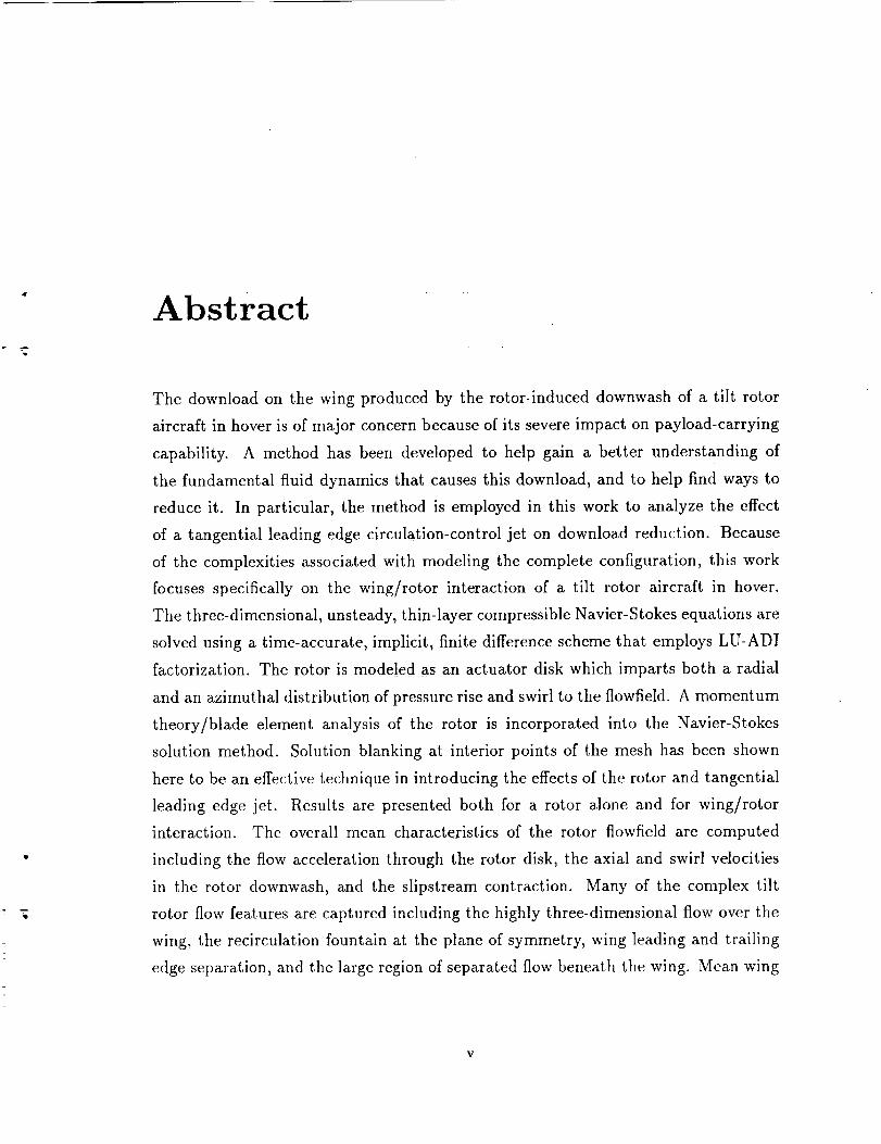
Measured variation in download with blowing plenum pressure (taken
from Ref. [2]) ............................... . . 18
Cross-sectional cut through mesh showing the concentration of grid
points around wing and rotor ........................ 49
Cutaway view of mesh showing wing and rotor locations ........ 50
Cutaway view of mesh showing the outer boundaries of the grid. . . 51
Exponential grid point stretching applied to an arbitrary curve. . . 52
Blow-up of the grid in the region of the leading edge at a typical wing
cross-section ................................. 52
Top view of grid points in rotor plane, superimposed with the outline
of the subdivided actuator disk ....................... 70
Relative velocities and forces at an elemental area of the rotor disk. 70
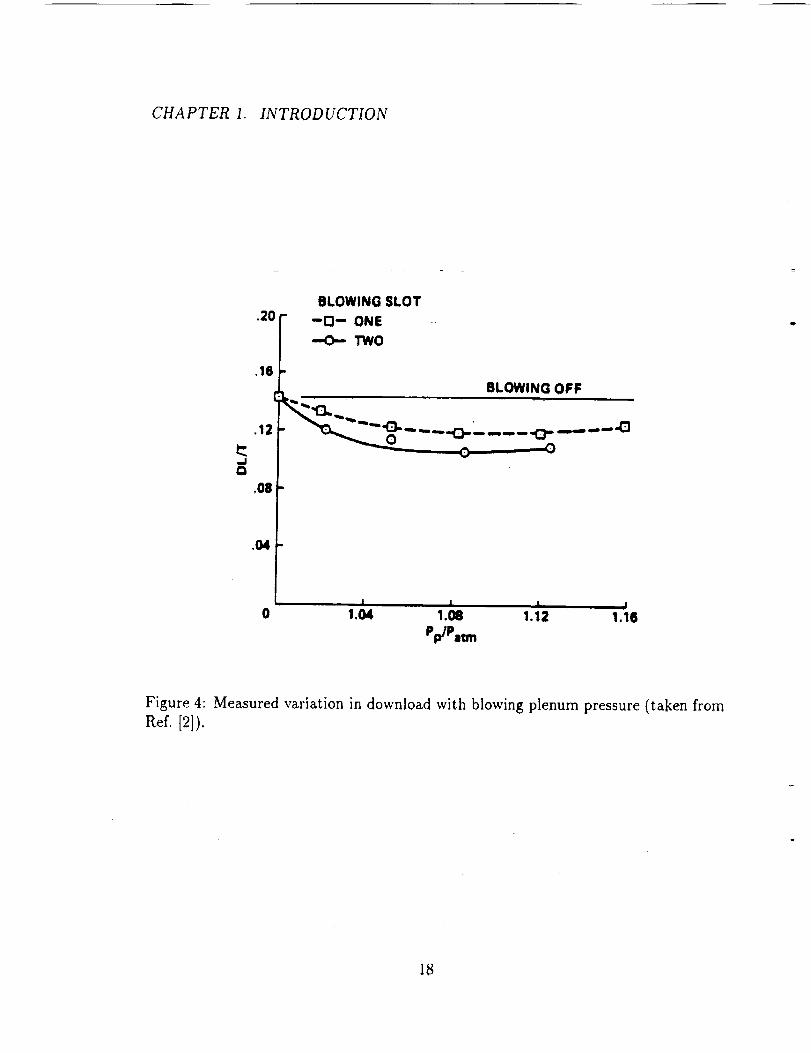
Blow-up of grid near the leading edge showing the inflow and outflow
boundary conditions implemented for the tangential jet ......... 71
Two views of the Cartesian grid used for the rotor alone computations. 100
Contours of pressure in a vertical plane through the rotor for a uni-
formly-loaded rotor with CT 0.0164. 101
Contours of velocity magnitude in a vertical plane through the rotor
for a uniformly-loaded rotor with CT _ 0.0164 .............. 101
vii

16 Velocity vectors in a vertical plane through the rotor for a uniformly-
loaded rotor with CT = 0.0164 ....................... 102
17 The blade chord and twist distributions used for the non-uniformly-
loaded rotor model .............................. 102
18 Radial distributions of blade loading and angle of attack for a non-
uniformly-loaded rotor with CT = 0.0164 ................. 103
19 Radial distributions of axial velocity V_ and swirl velocity Vt at the
rotor disk for a non-uniformly-loaded rotor with CT ----0.0164 ...... 103
20 Contours of pressure in a vertical plane through the rotor for a non-
uniformly-loaded rotor with CT = 0.0164 ................. 104
21 Contours of velocity magnitude in a vertical plane through the rotor
for a non-uniformly-loaded rotor with CT -" 0.0164 ............ 104
22 Top view of the velocity vectors projected onto horizontal planes im-
mediately above and below the rotor for a non-uniformly-loaded rotor
computation ................................. 105
23 Two views of the particle traces in the flowfield below a non-uniformly-
loaded rotor ................................. 106
24 Comparison of calculated and measured induced velocities about one
wing chord below the rotor disk ...................... 107
25 Comparison of calculated and measured values of figure of merit for a
range of thrust coefficients, for the rotor alone .............. 107
26 Perspective view of the velocity vectors for wing/rotor interaction with
uniform rotor disk loading -- in a near-vertical plane running spanwise
through the wing mid-chord ......................... 108
27 Velocity vectors in a vertical plane running spanwise through the wing
mid-chord, for uniform rotor disk loading. . ..... .......... 109
28 Contours of velocity magnitude in a vertical plane running spanwise
through the wing mid-chord, for uniform rotor disk loading ....... 110
29 Contours of pressure in a vertical plane running spanwise through the
wing mid-chord, for uniform rotor disk loading ............... 110
4'
VIII

30 Velocity vectors in a vertical plane running chordwise through 2y/b = 0.7,
for uniform rotor disk loading ........................ 111
31 Contours of velociiy magnitude in a vertical plane running chordwise
through 2y/b = 0.7, for uniform rotor disk loading ............ 112
32 Contours of pressure in a vertical plane running chordwise through
2y/b = 0.7, for uniform rotor disk loading ................. ll2
33 Comparison of the time history of the ratio download/thrust between
two- and three-dimensional computations ................. ll3
34 The computed oil flow pattern on the wing upper surface, for uniform
rotor disk loading .............................. 113
35 Schematic of installation of the 0.658-scale V-22 wing and rotor in the
NASA Ames 40- by 80-Foot Wind Tunnel (taken from [10]) ....... 114
36 Top view of the velocity vectors projected onto horizontal planes imme-
diately above and below the rotor for a wing and non-uniformly-loaded
rotor computation .............................. 115
37 The instantaneous particle traces in a near-vertical plane in the wing
root region showing the fountain flow, for non-uniform rotor disk loading.116
38 The computed oil flow pattern on the wing upper surface, for non-
uniform rotor disk loading .......................... 117
39 Sketch of the wing and rotor as seen from above, showing various span-
wise locations referred to in the discussion ................. 117
40 Velocity vectors in a vertical plane running chordwise through 2y/b = 0.7,
for non-uniform rotor disk loading ..................... 118
41 Comparison of wing surface pressures at 2y/b = 0.7 showing the effect
of swirl .................................... 119
42 Computed wing surface pressures compared with experimental results,
for non-uniform rotor disk loading ..................... 120
43 Comparison between computed and measured values of the normalized,
time-averaged download/thrust per unit span ............... 123
44 The azimuthal variation of several parameters, showing the influence
of the wing on the flow at the rotor disk at r/R = 0.60 .......... 123
ix

45 Close-up of velocity vectors near the wing leading edge at 2y/b = 0.7,
with and without blowing .......................... 124
46 Particle traces showing the wing wake at 2y/b = 0.7, with and without
blowing .................................... 125
47 The computed wing surface pressures at 2y/b = 0.7 with and without
blowing .................................... 126
48 The variation of download/thrust with plenum blowing pressure .... 126
49 The wing surface pressures in the region of the leading edge of the wing
at a spanwise location 2y/b = 0.15 for different blowing pressures. . . 127
50 The wing surface pressures near the leading edge at a spanwise location
of 2y/b = 0.7 for different blowing pressures ................ 127
51 Local download per unit span for a range of blowing pressures ..... 128

List of Symbols
a
A
b
B
C
%
C
Cd
Cl
Cr
D
DE, D_
DA, DB, DC
DL
e
ei
h
ib
speed of sound
flux Jacobian matrix in the _-direction; rotor disk area
wing span; distance normal to surface where V = V._a::/2 in a wall jet
flux Jacobian matrix in the r/-direction; number of rotor blades
wing chord; local rotor blade chord
specific heat at constant pressure
flux Jacobian matrix in the _-direction
2-D drag coefficient
2-D lift coefficient
rotor thrust coefficient
blowing momentum coefficient
drag on rotor blade segment
explicit and implicit artificial dissipation terms, respectively
diagonal matrices associated with the LU-ADI algorithm
download force
total energy per unit volume
internal energy pe r unit mass
inviscid flux vector in the _-direction
inviscid flux vector in the r#direction
inviscid flux vector in the _-direction
viscous flux vector in the (_-direction
time step size; height of tangential jet exit
integer equal to one or zero used for blanking the implicit solution
xi

I
J
k
l
L
LA, LB, Lc
M
M_
P
P,Q
Pr
Q
r
R
Re
t
T
U_ V_ W
UA,U ,Uc
U,V,W
V
Vm_x
at selected grid points
identity matrix
transformation Jacobian
coefficient of thermal conductivity
user-specified input constants for explicit and implicit artificial dissipation
turbulent mixing length scale
lift on rotor blade segment
lower bidiagonal matrices associated with the LU-ADI algorithm
viscous flux Jacobian matrix in the (-direction; Mach number
freestream Mach number
normal direction coordinate
pressure
source terms of the Poisson equations defined to provide
elliptic grid control
Prandtl number
rotor torque
vector of conserved quantities
rotor radial location
rotor radius; radius of curvature; gas constant
Reynolds number
time
rotor thrust; temperature
similarity transformation matrices
Cartesian velocity components
upper bidiagonal matrices associated with the LU-ADI algorithm
contravariant velocity components
velocity
local velocity normal to rotor disk
effective local velocity in plane normal to rotor radius
ideal induced velocity at the rotor disk in hover (= £tR_
maximum magnitude of velocity in wall jet
xii

local rotor swirl velocity
Cartesian coordinates
og
oq
7
A_, A,, A¢
V_, V n, V¢
£
0
A
AA
AB
Ac
#
P
o"
T
¢
¢
O3
local angle of incidence
local induced angle of incidence
rotor blade pitch angle
ratio of specific heats
central difference operators
forward difference operators
backward difference operators
artificial dissipation coefficient
local rotor blade twist angle relative to the twist at
the 75% rotor blade span location
coefficient of bulk viscosity
diagonal matrix of eigenvalues associated with the flux Jacobian matrix A
diagonal matrix of eigenvalues associated with the flux Jacobian matrix B
diagonal matrix of eigenvalues associated with the flux Jacobian matrix C
coefficient of viscosity
chordwise, spanwise, and normal coordinates in body-conforming system
density
spectral radius of flux Jacobian matrix
time coordinate in computational domain; viscous stress
local angle between freestream velocity and relative rotational velocity
(=0 in hover)
matrix of flux limiters for artificial dissipation model
azimuthal angular coordinate of rotor
vorticity
angular frequency of rotor rotation
xiii


-7
Chapter 1
Introduction
1.1 Motivation
The tilt rotor aircraft is a unique flight vehicle which combines the vertical takeoff and
landing capability of the helicopter with the efficient high-speed cruise performance
of conventional fixed-wing aircraft. This is achieved by positioning, at both wing tips
of a fixed wing, a rotor which can be tilted so as to provide lift for hover and thrust
for cruise flight.
The concept was first proposed by Bell Helicopter engineers during World War II,
and it evolved into a first prototype in 1955, designated the XV-3 [1]. In 1977, the
NASA/Army/Bell XV-15, a 13,000 lb experimental tilt rotor aircraft, flew for the
first time in a research program that continues today. The usefulness of the tilt rotor
aircraft is evidenced in the recent development of the V-22 Osprey for the U.S. Armed
Forces by a Bell Helicopter Textron/Boeing Helicopters team. The V-22 is a multi-
service, multi-mission tilt rotor aircraft. It has a vertical take-off weight of 55,000 lb
and is capable of transporting up to 40 passengers.
The tilt rotor vehicle with its unique features can also be exploited as a civil
transport in the city-center to city-center commuter market or as a feeder to hub
airports. The need for such a mode of transport will certainly increase as community
real estate prices continue to increase, making new airport construction prohibitively
expensive, driving new airport locations further away from large population densities.

CHAPTER 1, INTRODUCTION
The tilt rotor (in this report, "tilt rotor" refers to the entire configuration, i.e. the
airframe and the rotors, not just the rotors) offers several considerable advantages
over the rival tilt wing concept (in which the rotors and wing both rotate in the
transition from helicopter to airplane mode and back). Wing tilt requires additional
mechanical complexity resulting in increased structural weight to support the higher
concentrated wing/fuselage junction loads. Also, due to the large exposed frontal wing
area in hover, the tilt wing, in vertical flight in gusty wind or cross-wind conditions,
is much more susceptible to controllability problems than the tilt rotor.
A major limitation of the current tilt rotor configuration, however, is the aerody-
namic download imposed on the wing by the rotor flowfield when hovering. Because
the wing is fixed, the rotor flow, in hover, hits the wing near 90 degrees. The down-
load force on the wing has been measured and can be as large as 10 - 15 percent of
the total rotor thrust [2,3]. Assuming the payload-carrying capability to be about
25% of gross take-off weight, complete elimination of the download could increase the
effective payload by over 50%. The need for a thorough understanding, and the even-
tual reduction, of wing download, then, is the major impetus driving this theoretical
study on tilt rotor flowfields.
The flowfield about a tilt rotor configuration is very complex. The rotor, typically
located about one wing chord above the tilt rotor wing, induces a flow which is closely
coupled to the flow about the wing. The rotor flowfield itself is very complicated.
The rotor imparts not only a vertical downwash to the flowfield, but also, due to the
rotational motion of the rotor, a velocity tangential to the circumferential direction
called the swirl velocity. The outer portions of the rotor blades sec a transonic flow
which may, at very high tip speeds, even yield upper surface shocks and shock-induced
boundary layer separation. A spiraling wake vortex sheet is shed from each blade.
Regions of concentrated vorticity (tip vortices) which trail from the blade tips, also
propagate in a helical motion in the rotor wake interacting with the following blades
and also with the wing. On the tilt rotor wing upper surface there exists a large
region of nearly-stagnated flow. The flow is highly three-dimensional with essentially
a two-dimensional chordwise flow near the wing tip which becomes primarily spanwise
further inboard along the wing. Due to symmetry of the hovering tilt rotor flowfield,

CHAPTER 1. INTRODUCTION
the spanwise flow from both wings meets at the vehicle centerline and is redirected
upwards. Some of this rising column of air is re-ingested by the rotor thus creating a
large-scale recirculation pattern which reduces rotor performance. This flow pattern
has been termed the "fountain effect". Beneath the wing is a large region of unsteady,
turbulent, separated flow. Refer to Fig. 1 taken from Ref. [3] for simplified sketches
of the main flow features about a V-22 in hover.
As stated previously, the primary motivation for this work is to gain a better
understanding of the tilt rotor flowfield in hover with the hope that this would lead
to ways of reducing the download in future designs. The wing and the rotor and
their close proximity to each other is the principal contributor to wing download.
The effects of the fuselage, tail, and nacelle of the tilt rotor aircraft on download,
although perhaps not unimportant, are secondary. It is desired, in this study, to
analyze the principal features of the tilt rotor flowfield by solving the Navier-Stokes
equations. This allows the modeling of the physics of the flowfield far more accurately
than hitherto attempted. The state of the art, at this time, in the numerical solution
of these equations does not permit the simultaneous computation of the complete tilt
rotor aircraft. This current study, therefore, focuses on the Navier-Stokes solution of
wing/rotor interaction for a tilt rotor aircraft in hover.
1.2 Previous Work
1.2.1 Experimental Work
Flight test of the XV-15 [1,4] has yielded quantitative estimates of hover performance
including the effect of flap deflection on download. Figure 2 taken from Ref. [1] shows
the download (DL) normalized by the rotor thrust (T) plotted as a function of flap
angle. These measurements were taken at a sufficient height above the ground so
as to eliminate ground effect. The ratio DL/T is reduced from over 16% at zero
flap deflection to about 9% when the flaps are deflected to 67 °. With increasing
flap deflection, the download is reduced, due not only to the reduction of wing area
affected by the rotor downwash, but also to the reduction of vertical drag coefficient.

CHAPTER 1. INTRODUCTION
Superimposed on the same figure is a data point from a NASA outdoor test [9] of a
0.658-scale model of the V-22 rotor and wing. (This test is discussed further below).
To study the tilt rotor flowfield, the flexibility and control offered by wind tunnel
testing has been found to be very helpful. McCroskey et al. [5] measured the drag of
two-dimensioaal wind tunnel models of the XV-15 airfoil (a modified NACA 64A223)
with various flap and leading edge configurations. They found that the drag on the
airfoil in a freestream flow at -90 degrees was very sensitive to not only flap angle but
also the surface curvature distribution on the upper surface near the leading edge.
Increasing the flap angle reduces the frontal area thereby reducing the download.
The shape of the airfoil and flap also affect the vertical drag. A flat plate has a 2-D
drag coefficient about twice that of a circular cylinder. Increasing airfoil thickness
and camber, then, which tend to make the airfoil less like a flat plate and more like
a circular cylinder or ellipse, contribute to download reduction. Further discussions
on the effects of wing geometry on download can be found in a review of tilt rotor
download research by Fetker [6].
Maisel et al. [7] continued this 2-D experimental effort on the XV-15 airfoil by
examining the effects of several different flap and leading edge configurations on the
download. They found that reduction of "frontal" area resulting from flap deflection
accounted for less than half of the total download reduction. It was observed that
modification of the contours of the leading edge and of the flap had a significant
impact on download reduction by delaying flow separation. Increasing the curvature
on the flap upper surface and introducing a slat in front of the leading edge both
aided in reducing the download.
Also, it was found that the measured download was sensitive to variations in angle
of attack away from -90 ° . This demonstrates the need to include the effect of swirl
imparted by the rotor in any attempt to accural_eiy predict the download on an actual
three-dimensional tilt rotor configuration. Reference [7] also notes that the download
is fairly insensitive to the Reynolds number, at least in the range tested -- from
0.6x10⁶ to 1.4xl06. This indicates that uncertainties arising from the definition of the
Reynolds number appropriate for the wing/rotor configuration in hover should not
affect the results.
4

CHAPTER1. INTRODUCTION
Boeing has tested a powered tilt rotor model whose basic geometry was that of
a 0.15-scale V-22 Osprey. Some results of this test are reported in Ref. [8]. Flow
visualization verified the existence of chordwise flow on the wing upper surface near
the wing tip and spanwise flow further inboard. The recirculation pattern at the plane
of symmetry was observed, and due to re-ingestion of the fountain flow into the rotors,
a loss in rotor thrust at a given power setting was measured. The 0.15-scale model test
also served to evaluate the effect of changing the direction of rotor rotation on airframe
download. Regardless of rotation direction, download decreased with increasing flap
deflection. With the normal sense of rotation, i.e. the rotor blade passage above the
wing is from leading edge to trailing edge, minimum download occurred at a flap
deflection of about 75- 80 degrees and, thereafter, began to increase. This was due
to flow separation from the flap upper surface. With rotor rotation in the opposite
direction (trailing-to-leading edge), the download was lower at the low flap settings
and decreased continuously as the flaps were extended to beyond 90 degrees, reaching
the same minimum value as observed for the normal rotation direction. This difference
in behavior is due to the swirl in the rotor flowfield, and, in particular, the angle at
which the flow impinges on the wing. These experimental observations reinforce the
need to model the rotor swirl, if an accurate prediction of download is to be obtained.
Several experimental tests of a rotor alone in hover and of wing/rotor interaction
have been undertaken at NASA Ames Research Center. Results from large-scale
tests of a 0.658-scale V-22 rotor and wing conducted at the Outdoor Aerodynamic
Research Facility (OARF) at NASA Ames are reported in Refs. [2,3,9]. A similar test
of the 0.658-scale V-22 wing and rotor was undertaken in the 40- by 80-Foot Wind
Tunnel at Ames; results are reported in Refs. [10,11]. The rotor blade planform
differed slightly from that in the OARF test to reflect the evolving changes in the
V-22 design. These tests provided measurements of rotor performance, wing surface
pressures, and wing download. TheOARF test measured the performance of the rotor
alone. Rotor wake surveys showed the changes in the radial distribution of downwash
velocity for different rotor thrust coefficients. Higher thrust levels yielded greater
downwash velocities in the outer region of the wake than in the inboard portion of
the wake. At lower thrust coefficients, the effect was reversed -- the outer portions

CHAPTER 1. INTRODUCTION
of the wake had lower downwash velocities than the inboard region. The maximum
value of the rotor figure of merit for the isolated rotor was found to be 0.808. This
was reduced to 0.793 for the rotor in the presence of the wing, due to the region
of recirculating flow at the plane of symmetry. Flow visualization at the OARF
of the wing/rotor flowfield provided insight into the fountain flow and also clearly
demonstrated the transition of chordwise flow on the wing upper surface near the
wing tip to spanwise flow on the inboard portion of the wing. Both tests measured
the small reductions in the download/thrust ratio that were due to increasing rotor
thrust coefficient. Felker and Light [2] explained this effect as being due to the
variations in the radial distributions of velocity (or dynamic pressure) in the wake
due to changes in thrust coefficient. The inboard portion of the rotor wake contributes
mainly to the chordwise flow over the wing upper surface, and the outboard portion
of the wake contributes mainly to the spanwise flow. The local download on the wing
is greater in regions of chordwise flow than in regions of spanwise flow. Changes in
downwash distribution with rotor thrust coefficient CT, therefore, affect the relative
contributions of chordwise and spanwise flows to the total download. As the rotor
thrust coefficient increases, the dynamic pressure in the outboard portion of the
wake (near the wing root) increases, and consequently, the rotor dynamic pressure
distribution contributes more to the spanwise flow and relatively less to the chordwise
flow, resulting in a reduced download-to-thrust ratio.
In Ref. [2], Felker and Light describe their results from a 0.16-scale model test
of the Sikorsky S-76 rotor with two different wings -- (i) a conventional wing and a
25% plain flap, and (ii) a circulation control wing possessing slots near the leading
and trailing edges for boundary layer control using tangential blowing. As in the test
reported in Ref. [7], it was found that the download reduction due to increasing flap
deflection was due to a c0mb]nation of planform area reduction and the reduction of
drag coefficient due to the changing geometry.
Beneath the wing of a tilt rotor configuration in hover, there exists a large re-
gion of separated flow typical of bluff bodies, as previously described. Because the
static pressure in the separated flow region is generally somewhat less than freestream
ambient pressure, a suction force on the wing lower surface contributes to the total
6

CHAPTER 1. INTRODUCTION
download. By energizing the boundary layer using tangential blowing near the lead-
ing edge (where the flow is close to separating), it should be possible to move the
separation location further around the leading edge on the lower surface, by exploit-
ing the Coanda effect. This should reduce the chordwise extent of the separated flow
region below the wing and increase the lower surface pressure, thereby contributing
to download reduction.
In tests by Felker and Light [2] using the 0.16-scale circulation control wing,
however, it was found that most of the download reduction due to blowing was a
result not of movement of the separation location and increase of base (wing lower
surface) pressure, but of the decrease in pressure on the wing upper surface. The
measured increase in pressure on the lower surface (that is expected with movement
of the separation location towards the mid-chord) contributed only about 1/3 to the
total download reduction. It was also observed that the reduction in pressure on the
wing upper surface near the leading edge extended well aft of the location of the
blowing slot. The blowing jet, then, entrained part of the rotor downwash, reducing
the extent of near-stagnated flow on the wing upper surface, thereby contributing
significantly to the download reduction. Figure 3, taken from Ref. [2], shows typical
wing surface pressure distributions on- the circulation control wing with and without
blowing. The blowing slots were located at 3 percent and 97 percent of wing chord
on the upper surface, the former blowing towards the leading edge, the latter towards
the trailing edge. Figure 4, also taken from Ref. [2], shows the measured reduction
in download/thrust ratio (DL/T) for a range of total pressures of the blowing slot
supply plenum (used to control blowing jet velocity). The download/thrust was
reduced by as much as 26% with blowing at both slots. It was found that blowing
at the leading edge was particularly effective in reducing the download, contributing
about 65 percent to this total reduction due to blowing. As the plenum pressure was
increased beyond its optimum value, the d0wnload/thrust began to increase due to
the jet extending further along the airfoil surface, increasing negative pressures on
the lower surface aft of the leading edge.

CHAPTERI. INTRODUCTION
1.2.2 Theoretical Work
The discussion below focuses on the theoretical modeling of: (i) a wing/rotor, and
(ii) a rotor alone.
Wing/Rotor Modeling
Previous theoretical studies of airfoil and wing download in hover ha_re either solved
simpler fluid dynamic equations than in the current study or restricted the analysis
to two dimensions.
Clark and McVeigh in Ref. [12] and Clark in Ref. [13] describe the application of
a three-dimensional low-order panel method to a tilt rotor configuration. The rotor
was modeled as an actuator disk using source singularities, and the rotor wake was
represented by a time-averaged cylindrical vortex sheath. A blade dement model of
the rotor was used to feed time-averaged loading as a function of radial and azimuthal
location to the panel code which also contained a model of the wing. The wing was¢.
modeled simply as a cambered plate using a lattice of doublet singularities. More re-
cently, Lee [14] computed the 3-D tilt rotor flowfieid using an unsteady, time-marching
panel method. Wake filaments are shed from the edge of the rotor (modeled as an
actuator disk) as well as the wing leading and trailing edges. Both of the above panel
models were able to predict many of the overall tilt rotor flow features. Quantitative
results, however, because of the nature of the equations solved (Laplace's equation)
must be viewed with caution as separated flows cannot be accurately predicted with
this formulation without a priori knowledge of separation locations and total or dy-
namic pressures in the wake region. As found in the experimental work described
in Ref. [5], the separation location is very sensitive to leading edge curvature and
thickness. Also, swirl in the flowfield can cause early separation on the flap at a
considerable distance forward of the trailing edge. These important effects cannot
be accurately predicted using a panel method. Infact, in the above panel models,
the separation location was fixed at the wing leading and trailing edges. Download,
therefore, which is dependent on viscous effects, can only be accurately predicted
using an analysis which incorporates the effect of viscosity.

CHAPTER 1. INTRODUCTION
References [5,15] describe discrete-vortex seeding methods to calculate the un-
steady, 2-D flow around an airfoil at an angle of attack of -90 degrees, by solving the
vorticity transport equation. In Ref. [5], the wing is immersed in a freestream flow. In
Ref. [15], to study rotor/wing interaction, a rotor is modeled using constant strength
doublet panels which induce a normal velocity distribution. Since no integral bound-
ary layer calculation was coupled with the potential flow calculation, boundary layer
growth and separation location were not predicted. Separation location was specified
and a uniform base pressure on the wing lower surface was assumed. The methods
predicted the upper surface pressures fairly well but were incapable of accurately
calculating the lower surface pressure.
Raghavan et al. [16] performed 2-D laminar Navier-Stokes computations on the
XV-15 airfoil at -90 degrees angle of attack in a low Mach number and low Reynolds
number freestream flow. The converged solution showed a significant periodic un-
steadiness in the flowfield due to vortices shedding alternately from the airfoil leading
and trailing edges. The mean value of the computed unsteady download did not
correspond well with experimental measurements. This was again due to difficulty
in predicting the base pressure. The inability to accurately model turbulence in the
wake contributed to the observed discrepancies.
Stremel [17] computed the 2-D flowfield about a NACA 0012 airfoil with and
without a deflected flap, using a velocity-vorticity formulation of the unsteady in-
compressible Navier-Stokes equations. His unsteady lift and drag results compared
favorably with those of Ref. [16]. As the selected Reynolds number was 200, only
laminar flow was computed.
Since the flow over the tilt rotor wing is highly three-dimensional, two-dimensional
analyses such as those mentioned above are of limited usefulness. It is anticipated
that, in three dimensions, due to a less-constrained flowfield than in two dimensions,
the vortex shedding and turbulence in the wing wake will be reduced in strength,
and a more accurate prediction of the separated flow region beneath the wing will be
possible.
9

CHAPTER 1. INTRODUCTION
Rotor Modeling
As mentioned earlier, the flowfield of a lifting rotor alone in hover is very complicated.
Each blade can be viewed as a rotary wing that sheds a sheet of vorticity in the form
of a thin wake which trails the blade in a helical pattern. The change in blade
loading occursmostiy at the blade tip. :Much of the_rot0r wake vorticity, i_herefore,
is concentrated in tip vortices which propagate in helices below the rotor disk. It
is the combined effect of the vorticity in the wakes from all blades (in addition to
the bound vorticity on the blades) that induces the axial and rotational motion in
the rotor flowfield -- i.e. the downwash and swirl. The acceleration of the flow
beneath the rotor gives rise to contraction of the rotor flowfield. Characteristic of
the rotor flowfield in hover is the close proximity of the wake shed from one blade
to the following blades. These interactions can have a significant impact on local
blade loading which affects overall rotor performance (see any text on helicopter
aerodynamics; for example, Johnson [18]). Although all features of the flow physics
can be accurately modeled only with the Navier-Stokes equations, the rotor flowfield
has been modeled using a wide range of methods of varying complexity and accuracy.
Application of momentum theory, or a combination of momentum theory and
blade element analysis, to an actuator disk representation of the rotor provides a
time- and space-averaged approximation of the rotor loads and the resulting induced
velocities in the rotor downwash. The local effect of shed vorticity on the following
blades is not computed. Prescribed wake and free wake hover analysis methods
model the wake as vortex sheets and filaments. In the prescribed wake approach the
wake geometry is specified from experimental data; the free wake approach computes
the force-free positions of the vortices. These two methods, in wide use today, are
commonly coupled with lifting line or surface representations of the rotor blades.
They are valid only for incompressible, potential flows.
The transonic flow on the blades can be computed by solving the full potential
equation. This typically requires a finite difference or finite volume solution method
which uses a grid around the rotor blades. Because the full potential equation does
not allow for the convection of vorticity, modeling a free vortex wake within the finite
difference domain must be modeled in Lagrangian fashion where the Biot-Savart law
10

CHAPTER 1. INTRODUCTION
is used to compute the induced velocities.
The Euler equations permit the transport of vorticity and are therefore better
suited to the computation of blade/vortex sheet interaction. Ideally one would use the
Euler or Navier-Stokes equations to model the complete rotor flowfield including not
only the near-field region around the rotor blades but also the wake region extending
below the rotor. Current computer limitations, however, do not permit the solution
at the huge number of grid points that would be required to model the flowfield near
each blade and the thin vortex sheets and highly concentrated tip vortices that extend
far below the rotor. Coarse grids, which might be manageable in terms of available
computer resources, are not only unable to resolve the concentrated vorticity, but
also introduce unwanted numerical dissipation. This causes excessive, non-physical
diffusion of the vorticity leading to inaccuracies in the overall solution.
In Ref. [19], Stremel developed a method to compute the two-dimensional, time-
dependent evolution of a vortex wake behind a wing. His velocity-vorticity formula-
tion for the Euler equations permitted the computation of solutions that were rela-
tively independent of grid size. This is an important requirement for future methods
in three dimensions that would allow accurate vorticity transport on coarse meshes.
Stremel, in Refs. [20,17], extended the method to a velocity-vorticity formulation of
the unsteady incompressible Navier-Stokes equations. The convection of finite-core
vortices on a coarse mesh was combined with the viscous solution on a fine mesh
around a 2-D body. The method allowed for the distribution of the interacting vor-
tices onto the fine mesh.
Using a somewhat different approach, Srinivasan and McCroskey [21] computed
airfoil/vortex interaction in two dimensions. They simulated the situation where the
shed tip vortex of a rotor blade is parallel to a following blade. They solved the
2-D Euler and Navier-Stokes equations in a perturbation, conservation law form in
primitive variables. They refer to their method as a prescribed-vortex or perturbation
approach where the structure of the vortex is prescribed. The vortex is convected
through the flowfield without being diffused by the numerical dissipation that is
inherent in the computational method.
Methods of preserving vorticity on coarse grids are currently being developed for
ll

CHAPTER 1. INTRODUCTION
three-dimensional applications. Typically, however, current rotor flowfield computa-
tions eliminate the problems associated with numerical diffusion inherent in the finite
difference solution of wakes by modeling the wake region below the rotor using a pre-
scribed or free wake analysis. This wake model is then coupled to a near-field Euler
or Navier-Stokes solution around the rotor blades.
For example, Agarwal and Deese [22] solved the unsteady Euler equations for a he-
licopter rotor in hover using an explicit, finite volume method. The effect of the wake
on the rotor was computed using a free wake analysis to determine a correction applied
to the geometric angle of attack of the blades due to the local induced downwash. In
a similar approach, Roberts [23] coupled an explicit, finite volume Euler solver with a
free wake model for a two-bladed hovering rotor. The bound circulation distribution
along the span of each rotor blade was determined from the Euler solution and used
to set the strength of the wake vortices. The effect of the wake was introduced into
the Euler solution by using the wake-induced velocities to define the required outer
boundary conditions. Also, the local effect of the trailing vortices was modeled using
a prescribed flow perturbation scheme, similar to that implemented in Ref. [21].
Quasi-steady solutions of a 2-bladed rotor in hover have been obtained by Srinivasan
and McCroskey [24] using a flux-split, approximately-factored, implicit algorithm to
solve the unsteady, thin-layer Navier-Stokes equations. The computation of the vor-
tices shed from the rotor tips is affected adversely by numerical diffusion due to
insufficient grid density beneath the rotor. The effect of the shed vorticity in the
rotor wake, and in particular, the induced downwash, was estimated in a similar
fashion to Ref. [22], where a correction to the effective local angle of attack of the
hovering blades was made. In Ref. [25] Srinivasan et al. computed the viscous, three-
dimensional flowfield of a lifting 2-bladed helicopter rotor in hover without resorting
to any wake models. An upwind, implicit, finite-difference method was used to solve
the thin-layer Navier-Stokes equations in a computational domain of limited size that
extended only 8 rotor blade chords in all directions. Fine-grid (nearly one million
points) results for blade surface pressures Corresponded well with experiment, and
the roll-up of the tip vortex was computed. This computation, although very impres-
sive, took about 15 CPU hours on the Cray-2 supercomputer. Due to the limited
12

CHAPTER1. INTRODUCTION
computational region, a solution was obtained for only two revolutions of the rotor
wake before the flow exited the downstream boundary. The results compare more
favorably with experiment than those of Ref. [24]. Further work is required, however,
to resolve important issues such as rotor drag and power, and detailed wake geometry.
In a computationally less demanding approach, Rajagopalan and Mathur [26]
modeled a three-dimensional rotor in forward flight using a distribution of momentum
sources added to the steady, incompressible, laminar Navier-Stokes equations. Rotor
geometry and blade sectional aerodynamic characteristics were incorporated into the
evaluation of the source terms. Their results represent a time-averaged solution. Shed
vortex details were not resolved due to the coarseness of the grid. In complexity,
this method lies between an actuator disk representation where the blade loads are
averaged over the rotor disk and an Euler (or Navier-Stokes) computation of the
individual blades.
McCroskey and Baeder [27] estimated that in order to calculate two revolutions of
a two-bladed rotor above a simple fuselage using a typical, implicit, thin-layer Navier-
Stokes code with algebraic eddy-viscosity modeling of turbulence, a i00 megaflop
computer would require 40 CPU hours and 30 million words of memory ( or 4 hours of
CPU for a one gigaflop machine). It is clear then, that accurate, routine calculations
of 3-D rotorcraft flows including detailed modeling of the rotor blades will remain
elusive for some time.
1.3 Current Approach
Despite the research efforts of the past several years, gaps in our fundamental under-
standing of the tilt rotor flowfield remain. It is the objective of this current work,
then, to gain a better understanding of this complex flowfield, by modeling it using
current computational fluid dynamic (CFD) techniques. It is hoped that many of the
limitations imposed by the previously-described two- and three-dimensional methods
applied to the tilt rotor flowfield may be removed. In particular, it is desired to
compute the wing download of a tilt rotor aircraft in hover, and to study the effects
of tangential blowing on download reduction. As can be inferred from the previous
13

CHAPTER 1. fNTRODUCTION
section, however, accurate, simultaneous, numerical prediction of all the tilt rotor
flow features discussed in Section 1.1 still lies beyond the state of the art. To render
the problem tractable, simplifications are made. Only the wing and rotor are mod-
eled. The fuselage, tail, nacelle, and rotor hub of the tilt rotor aircraft are neglected.
Study of the three-dimensional wing/rotor interaction of a tilt rotor configuration
in hover, then, is the primary focus of this work. Since accurate modeling of the
flow about the individual rotor blades and of the vorticity in the wake is a complex
task and a tremendous computational drain, and since the primary interest here is
in wing download prediction and not in detailed rotor simulation, the rotor modeling
is simplified in this study. The rotor is modeled as an actuator disk where the blade
loads are averaged over elemental areas of the rotor disk.
Flow separation from the wing leading edge and from the flap, caused by signifi-
cant viscous effects, creates a large region of separated flow beneath the wing. This
region of the tilt rotor flowfield has a significant impact on wing download. Thus, the
Navier-Stokes equations, which model the viscosity in the flow, are used to describe
the flowfield. The form of these equations and the method of solution employed in this
study are discussed in the next chapter. The flow equations are discretized and solved
on a mesh of grid points. Chapter 3 is devoted to a discussion of the development of a
suitable 3-D mesh that possesses grid point distributions which permit the resolution
of not only the large-scale tilt rotor flowfield features but also the smaller-scale fea-
tures of the flow about the wing including the boundary layer and flow separations.
Chapter 4 discusses the implementation of the boundary conditions required by the
Navier-Stokes equations. The unique manner in which the rotor is modeled as an
integral part of the Navier-Stokes solution is also discussed. The implementation of
the tangential blowing jet is also described. Chapter 5 presents computed results of a
rotor alone as well as wing/rotor interaction and compares them with some existing
experimental data. Results which show the download reduction effect of tangential
blowing are also presented. The final chapter, Chapter 6, summarizes the conclusions
drawn from this work and outlines some near and longer term recommendations for
further work.
14

CHAPTER1. INTRODUCTION
RECIRCULAT|ON jFOUHTAIH MOMEHTUM
W|HG BLOCKIGE
Figure 1: Sketches of the V-'22 in hover, showing the main flow features.
15

CHAPTER 1. INTRODUCTION
1 8 l--I SYMBOL FLIGHTE
I o 231i_ D 232 1 xv-ls
_e I-\ A 238 _ FUGNTTEST
I \ _ 2,o.i 0AT,I \ o ,4_ "__ _ J_ NASA AMES OARF
_ ,oI GW---13.300 LB
8 _ h/D--- 2.5I 0.25c FLAPS
I6
I [ I I I I0 20 40 60 80 100
Flap Angle (_F) (Deg.)
Figure 2: Effect of flap angle on download (taken from Ref. [1]).
16

CHAPTER 1. INTRODUCTION
Er
r
i
0 .2 .4 .ll .I 1.0,,Ic
(b) blov/n E on, Pp/ParJi " 1.09.
Figure 3: Typical surface pressure distributions measured on a circulation control
wing with and without blowing (taken from Ref. [2]}.
17
CHAPTER1. INTRODUCTION
BLOWING SLOT
.20 I" -El- ONE =
/ •-..O-- TWO
"16(E::,,,, BLOWING OFF
"p_'{3.. .. ...12 "" ' --._ ---""(_)
o
.08 _-
! I I ,I
0 1.04 1.08 1.12 1.16
Pp/Patm
Figure 4: Measured variation in download with blowing plenum pressure (taken from
Ref, [2]).
18

Chapter 2
Flow Equations and Solution
Method
2.1 General Comments
In this study the flowfield about a tilt rotor configuration is represented by the
unsteady thin-layer Navier-Stokes partial differential equations. It is assumed that
there are no body forces (eg. gravity effects are not important) and there is no heat
addition or removal. The thin-layer approximation, described later, assumes that
the viscous forces are confined to a small region near the wing surface. The basic
solution algorithm, employed to solve the equations, is referred to as the LU-ADI
scheme developed by Obayashi and Kuwahara [28]. It was extended and applied in
a Fortran computer code called "LANS3D" to a three-dimensional transonic wing
calculation [29] and a wing-fuselage transonic flow computation [30] by Fujii and
Obayashi. Yeh et al. applied this code to the Navier-Stokes computation of the flow
about a delta wing with spanwise [31] as well as tangential [32] leading edge blowing
used to control vortex shedding.
The solution algorithm, then, has been shown in the above-mentioned references
to be robust and efficient for thin-layer Navier-Stokes computations. Although the
numerical time integration is performed in an implicit fashion, the boundary con-
ditions are updated explicitly. This allows easier application of the method to a
19

CHAPTER 2. FLOW EQUATIONS AND SOLUTION METHOD
wide variety of geometries and grid topologies. It was therefore decided, for the re-
search undertaken in this current work, to utilize the basic numerical scheme imple-
mented in that version of "LANS3D" previously applied to delta wing computations
by Yeh et al. [31,32,33]. Much of the effort involved in the research reported here
has focused on implementing and extending the above method to model the current
problem of interest -- the tilt rotor flowfield in hover.
This chapter outlines the basic formulation of the equations and their method of
solution. Greater details of the basic numerical algorithm can be found in Refs. [28,
29,30,33]. Also discussed in this chapter are the modifications to the basic solution
algorithm that were implemented to provide an effective mechanism for modeling the
rotor and also the tangential jet on the wing surface. These modifications involve
exploiting the "blanking" feature of the so-called "chimera" technique [34]. This is
described in more detail later in this chapter and in Chapter 5. Also outlined briefly
in this chapter are the turbulence models employed for the general flowfield about
the wing and in the region of the tangential jet.
2.2 Governing Equations
The Navier-Stokes equations are the most basic continuum-representation of fluid dy-
namic flows. The equations are written and solved in conservation-law form where the
dependent variables are expressed in the form of spatial gradients (see, for example,
Refs. [33,35]). Although not particularly significant in the current low Mach num-
ber application where the locally-transonic rotor blade flow is not computed, the
conservation-law form ensures proper shock capturing (i.e. accurate prediction of
shock location and strength) for transonic flows. To convert the equations to a more
useful form for computational purposes and to apply the thin-layer approximation,
the full three-dimensional Navier-Stokes equations are first manipulated somewhat,
as described below.
For convenience, the equations are non-dimensionalized. The density p is divided
by the freest_eam density p_, the velocity components u, v, and w by the freestream
2O

CHAPTER 2. FLOW EQUATIONS AND SOLUTION METHOD
speed of sound aoo, and the total energy per unit volume e by po_aoo.2 Conform-
ing to the normal convention, u is in the wing chord (x) direction (positive aft),
v is in the wing spanwise (y) direction (positive outboard), and w is in the verti-
cal (z) direction (positive upwards). The coefficient of viscosity # is normalized by
#oo and the time is normalized by c/aoo where c is the wing chord. Applying this
non-dimensionalization to the Navier-Stokes equations results in a term containing
the expression (pooaooc)/#_ which is simply the Reynolds number Re based on the
freestream speed of sound.
Next, the Navier-Stokes equations are transformed from Cartesian coordinates
(z, y, z, t) to a generalized, body-fitted, curvilinear coordinate system (_, _?, (, r). This
makes the formulation independent of the body geometry thereby easing the specifi-
cation of the boundary conditions. It also allows for straight-forward application of
the thin-layer assumption. In addition, since the physical domain is transformed into
a computational domain which is a rectangular parallelepiped with uniformly-sized
mesh cells, then standard differencing schemes for equi-spaced grid points can be used
for the spatial derivatives. The coordinate transformation is defined by:
=
=
¢ =
T _ t
(1)
where t and r are the independent variables of time in the physical and transformed
coordinates, respectively. The airfoil surface in the chordwise direction is transformed
to the _-coordinate, the spanwise direction is transformed to 77, and _ is normal to the
wing surface. Details of this transformation procedure can be found in Refs. [36,37].
By writing the transformation in terms of spatial derivatives and applying the chain
rule, a transformation Jacobian J and several identities called metrics can be defined
as follows:
J = 1/det
x_ xn x i
Y¢ Yn Y_
z¢ zn z_
(2)
21

CHAPTER 2. FLOW EQUATIONS AND SOLUTION METHOD
where xe - cOx/O_, x, 7 = Ox/OT h etc. The metrics are given by:
= J (y,z¢ - yez,),
= J (x,y¢ - z¢y,),
_ = J (yez_ - y_z¢),
_y = J (x_z¢ - x¢z_),
yz = J (xey¢ - x_y¢),
(:_ = J (y_z,7 - y,Tz_)
(y = J (x,ze- x¢z,)
5 = J (z_y, - x,Ty_)
rh = -x_?_: - y_-y_ - z_-_,
(3)
Note that for stationary grids (no body motion), the metric time derivative terms are
zero. From a finite volume point of view, the transformation Jacobian J is the inverse
of the local grid cell volume, and the metrics are grid cell area projections.
Generally, for aerodynamic applications of practical interest (particularly in three
dimensions), the thin-layer approximation is applied to the Navier-Stokes equations
to reduce the computational effort. For the relatively high Reynolds numbers which
are typical of such problems, the viscous effects are confined to a small region near
the body surface and in the wake. Computer memory limitations usually necessitate
concentrating the available grid points near the surface of interest in order to resolve
the boundary layer. This results in grid spacing that is fine, normal and near to the
surface, and that is relatively coarse, tangential to the surface. With this type of grid,
even if the full Navier-Stokes equations were solved, the viscous terms possessing ve-
locity gradients tangential to the body would not be resolved because of insufficient
grid density along the surface. For most cases of interest (i.e. high Re flows), however,
these terms are negligible anyway. Therefore, it is justifiable to eliminate from the
calculation the viscous fluxes associated with the directions parallel to the surface,
i.el the _- and 7- directions. This approximation is easily applied since the equations
are already transformed into the body-fitted computational domain. The thin-layer
approximation is similar in philosophy to the assumptions made in boundary layer
theory. Less restrictive than boundary layer theory, however, the thin-layer approxi-
mation retains the normal momentum equation and allows pressure variation across
the boundary layer.
22

CHAPTER 2. FLOW EQUATIONS AND SOLUTION METHOD
Beneath the wing of the tilt rotor configuration in hover the flow is turbulent,
unsteady, and separated, as mentioned in Chapter 1. In such a flow, all components of
the viscous stress exist and are probably important and shouldn't be neglected. This,
then, is one of the major limitations of the present method for studying the tilt rotor
flowfield. Even if the full Navier-Stokes equations were solved, however, limitations of
the turbulence model (discussed in the next section) in regions of extensive separation
would contribute to inaccuracies in the computed flowfield. Nonetheless, the current
approach makes the calculation tractable and far superior to any method hitherto
applied to this problem.
Applying the thin-layer approximation, then, the non-dimensional, three-dimen-
sional, unsteady Navier-Stokes equations in conservation-law form in transformed,
body-fitted, curvilinear coordinates become:
where the symbol '^' indicates transformed variables. The O vector contains the
transformed, conservative flow variables:
F! PIi pu
_= j-1 pv
pw
Note that the elements of the Q vector, as well as all flow variables referred to in
subsequent discussions in this chapter, are non-dimensional quantities, unless noted
otherwise.
The vectors/_, F and G contain the inviscid (or "Euler") terms. The vector G_
contains all the viscous terms that remain after application of the thin-layer approx-
imation. The elements of these Vectors arcshown below:
23

CHAPTER 2. FLOW EQUATIONS AND SOLUTION METHOD
1
1
0= 7
pU
puU + Gp
pvU + GP
pwU + Gp
(_ + p)u - (,v
pW
puW + GP
pvW + GP ,
pwW + Gp
(_+ p)W -¢,p
1
P=7
pV
puV + rb:p
pvV + flup
pwV + rl_p
(e + p)V - rhp
0
Gr_ + (_r_ + Gr_
gS. + g& + gS,
(6)
where p is the static pressure and U, V, and W are the contravariant velocity com-
ponents that appear as a result of the coordinate transformation. The contravariant
velocity U is the component of velocity parallel to the wing surface and in the direc-
tion of the wing chord, V is the component of velocity in the spanwise direction, and
W is normal to the wing surface. They are given below:
V =
W =
_ + Gu + Gv + &w
rh + r/xu + r/_v + r/_w
6 + 6,u + 6v + 6w
The components of the viscous stress are defined by:
2
r._ - 3#(u. + vy + wz) + 2#u.
2
2
rz. = -_(u_+v_+wz)+2#w_
r_ = ry_=U(u_+v.)
r,= = _-_x=_,(u_+w_)
r_ = r_= l_ (v. + w_)
fix -- "lit Ozei "t- u'rz_ -t- VTx_ + wrxzPr
(7)
(8)
24

CHAPTER 2. FLOW EQUATIONS AND SOLUTION METHOD
,,/#fl_ - p----_O_e_+ ur** + vr_ + wr_,
"y#_ - -_rO_e_ + ur= + vrz_ + wr_z
where u_ = Ou/Ox, vy = Ov/cgy, cg_e_ = cge_/cgx, etc. From the definition of the total
energy e, the internal energy per unit mass is
e (u 2 + v2 + w 2)
p 2
The Prandtl number Pr is defined as Pr = %#/k where cp is the specific heat at
constant pressure and k is the coefficient of thermal conductivity. Also, 3' is the ratio
of specific heats which, for air, is equal to 1.4. Pressure is related to the conservative
flow variables through the equation of state for a perfect gas:
-P v2 w2)] (9)p= (7- i) [e _(u=+ +
To evaluate the spatialderivativesof the Cartesian velocitycomponents in Eq. 8, the
chain rule is applied. For example,
u_ = _u¢ + rl_u , + _u¢
Implicit in the expressions for the viscous stresses (Eq. 8) is the assumption that
the fluid is Newtonian (viscous stresses are linearly related to the rate of strain) and
that its properties are isotropic (having no preferred direction), and that it satisfies
Stokes' hypothesis which states that the bulk viscosity (), + 2/3#) is zero. Experience
of many researchers over many years has shown that these assumptions are valid for
most flows of aerodynamic interest.
2.3 Turbulence Model
The unsteady Navier-Stokes equations are generally considered to accurately repre-
sent the physics of turbulent flows. In order, however, for a numerical solution of
these equations to resolve all scales associated with the turbulent eddies for large
Reynolds number flows, an extremely dense grid spacing resulting in a huge number
25

CHAPTER 2. FLOW EQUATIONS AND SOLUTION METHOD
of grid points would be required. Because of computer memory and speed limitations,
grids can not be made fine enough to fully capture the turbulence in the flow. It is
therefore necessary to use models for simulating turbulence.
The approach employed here is commonly taken for large Reynolds number 3-D
compressible Navier-Stokes computations. The Navier-Stokes equations are time-
averaged using a mass-weighted variable approach (refer, for example, to Ref. [38]).
The velocities and thermal dependent variables such as temperature and enthalpy are
split into a mass-averaged mean-flow part and a mass-averaged fluctuating quantity.
The pressure and density are defined as having a mean-flow part and a fluctuating
contribution which is not mass-averaged. Time-averaging gives rise to new terms in
the resulting "Reynolds-averaged" Navier-Stokes equations. These new terms can be
interpreted as "apparent" stress gradients and heat-flux quantities due to turbulent
motion. The turbulent stresses are commonly referred to as Reynolds stresses. Ap-
plying the Bousinesq assumption which relates the Reynolds stresses to the rate of
strain, the effect of turbulence can be approximated by an effective viscosity often
called "eddy" viscosity that is due to the additional mixing caused by the turbulent
flow. This turbulent viscosity model is far less demanding computationally than more
complicated (and more or less accurate) approaches which typically require the solu-
tion of additional differential equations that model the characteristics of turbulence.
To limit the computational requirements of an already demanding three-dimensional
problem, a simple algebraic turbulence model, discussed in'the next section, is em-
ployed in this work. The total effective viscosity can then be defined as the sum of a
laminar contribution (#t) and a turbulent part (#t):
# = #l + #t (10)
The laminar viscosity contribution is determined from Sutherland's formula:
( T _3/2 T,_I + 198.6OR (11)/u, =/_r,! k,T--_-,/] T + 198.6°R
where T is the temperature in degrees Rankine (°R). The turbulent contribution to
viscosity #t is obtained from the algebraic turbulence model.
26

CHAPTER 2. FLOW EQUATIONS AND SOLUTION METHOD
Similarly, the total effective coefficient of thermal conductivity is expressed as:
k = k_+kt
_ cv#t + cv#---A (12)Prl Prt
For the range of temperatures and pressures of interest here, for air, the laminar
Prandtl number Prl is 0.72 and the turbulent Prandtl number Prt is 0.90 (see, for
example, Ref. [38]).
An algebraic turbulence model developed by Baldwin and Lomax [39] for bound-
ary layers has been employed for the computations undertaken in this study. It is
applied to the flowfield around the wing. Because jet flows possess somewhat dif-
ferent turbulence characteristics, another turbulence model more appropriate for the
blowing region is used. An eddy viscosity model proposed by Roberts [40] for tur-
bulent wall jets on curved surfaces is implemented. These two turbulence models
are discussed briefly below. Based on a combination of theory and empiricism, these
models, although far from precise predictors of turbulence, do provide a means of
improving the simulation of a real flow.
2.3.1 The Baldwin-Lomax Model
The eddy viscosity model of Baldwin and Lomax [39] is in common use today for
estimating the effect of turbulence in aerodynamic flows. It uses a two layer formu-
lation that includes an inner region (where the wall has a considerable influence on
eddy size) and an outer region.
The eddy viscosity in the inner region is estimated using the Prandtl-Van Driest
formulation:
where is the magnitude of the vorticity (IV × t31) and l is the "mixing" length
scale. In the outer region, the eddy viscosity is written as
(#t)o,.,t_,. ,:x g,_a_: ¢,_ (14)
where Fm._ and {m._ represent the turbulent velocity and length scales in the outer
part of the boundary layer. The quantity F,_._ is the maximum value of the following
27

CHAPTER 2. FLOW EQUATIONS AND SOLUTION METHOD
function:
r(<;)= ¢1< 1[,- exp(-<;+/A+)]
where (+ = ( px/-p-__r_/Vw and the subscript w represents the conditions at the wall.
A + is a constant equal to 26, and ( is the distance of a point in the flowfield normal
to the nearest solid wall. The value ¢',_, is the _-location where F(_) reaches a
maximum in a given velocity profile. In wake regions, because of the relatively-large
distance from the wing surface, ¢'+ becomes increasingly large and the exponential
term of Eq. 15 approaches a value of zero. As suggested by Baldwin and Lomax, for
points in the wake, the exponential term is omitted. For the download computation,
this is applied to all points beneath the wing in the wake.
2.3.2 Turbulence Model for Wall Jet
The algebraic turbulence model, briefly described here, is used in the region of the
thin, tangential jet on the wing surface. Based on a semi-empirical theory by Roberts
[40], it was previously applied by Yeh [33] in the numerical study of delta wing leading
edge blowing.
Assuming self-similar velocity profiles typical of free jet flows, Roberts obtained a
simple expression for the eddy viscosity of a wall jet:
K Vm_, b (16)#t = 4k----_
where K = 0.073 and k = 0.8814. Also, Vma, is the maximum value of the mag-
nitude of velocity in a given velocity profile. Here (_,_, represents the (_-location
corresponding to V,_,. The parameter b is the normal distance from the wall to the
_-location where the velocity is V,_a,/2. Experiments have shown b to have a value
of about 7(_,_,. For (_ > _ma,, ¢'/(,_, is set to one.
Surface curvature causes extra rates of strain in the flow which affect the tur-
bulence structure by influencing the radial distribution of velocity fluctuations. Ac-
cording to Shrewsbury i41], this can increase the effective viscosity by an order of
magnitude greater than planar flows. The ratio - (V/R)/OV/O( represents the extra
rate of strain produced by the curvature normalized by the inherent shear strain,
28

CHAPTER 2. FLOW EQUATIONS AND SOLUTION METHOD
where R is the radius of curvature. This effect is added to the jet-induced viscosity
of Eq. 16 to obtain an estimate for the eddy viscosity of a curved wall jet:
7K Vm,,_(m_,_: _,(m,,_] _,l OY/c3(](17)
/tt - 4k 2
This turbulence model for the jet is applied in the region of the wall jet from the jet
exit slot to the flow separation point.
2.4 Numerical Algorithm
The numerical algorithm used here to solve the three-dimensional compressible thin-
layer Navier-Stokes equations is an implicit, time-accurate, finite difference scheme
developed by Fujii and Obayashi [29,30]. The algorithm has been extended in this
work to allow the "blanking out" or excluding of specified regions of the compu-
tational domain from the implicit solution. Values of the solution vector at these
blanked (excluded) locations are then updated explicitly using values obtained from
an independent analysis. This is a very convenient and effective means of modeling
the rotor, as is discussed in greater detail later. The numerical algorithm is briefly
outlined below.
The solution technique employs an implicit, approximately-factored, non-iterative
method developed by Beam and Warming [42]. Explicit methods suffer the disadvan-
tage of having a severe restriction on time step size in order to maintain stability. This
is particularly acute for Navier-Stokes solutions where, because of the relatively small
scales associated with resolving the boundary layer, the partial differential equations
are very stiff. Often, the steady-state solution is of principal interest, so being able to
use large time steps to accelerate the rate of convergence is very important. Implicit
methods are stable for relatively large time steps even for highly nonlinear equations
such as the Navier-Stokes equations.
A first-order accurate implicit time integration scheme is selected to march the
solution of the unsteady Navier-Stokes equations in time. A second-order accurate (or
higher) scheme is not used as it would necessitate saving the solution from previous
time levels, resulting in a significant increase in the computer memory requirements.
29

CHAPTER 2. FLOW EQUATIONS AND SOLUTION METHOD
The method, as used here, already requires considerable memory for 3-D computa-
tions. Applying, then, to Eq. 4, the first-order accurate numerical time integration
method referred to as the implicit (or backward) Euler scheme (not to be confused
with the "Euler" fluid dynamic equations) yields
@+1-0"+h\ 0¢ + 0----_ + 0¢ n_ 0¢ ]
where h is the time step, n + 1 is the time at which 0 is desired, n is the previous
time level at which 0 is known everywhere, and 0"` = O(nh).
Since the flux vectors/_,/O, (_, and G, are nonlinear functions of Q, then Eq. i8 is
nonlinear in 0 TM. In order for the solution method to be non-iterative, so as to limit
the computational effort to a manageable level, the nonlinear terms are linearized in
time about 0 '_ by a Taylor series expansion such that
n+l
_n+l
n+l
Note that A0"` = 0 "+1- O"-
matrices given by:
0_A n _
00'
= /_'`
= _'_
Also,
')
(19)
A _, B ", C ", and M'` are the flux Jacobian
0F 0d 0d_- C '_ - M" - . (20)
B_ 00' 00' OQ
where the symbol '^ ' has been omitted from the flux Jacobian matrices for simplicity.
Expressions for these matrices can be found in Ref. [43].
In the Beam and Warming method, the alternating direction implicit (ADI) al-
gorithm replaces the inversion of one huge matrix -- which would be prohibitively
expensive to compute -- with the inversions =of three block tridiagonal matrices, one
for each direction. Efficient block tridlagonal inversion routines exist, making this
algorithm a viable solution technique. Substituting the linearizations of Eq. 19 into
Eq. 18 and applying the Beam-Warming approximate factorization yields
3O

CHAPTER 2. FLOW EQUATIONS AND SOLUTION METHOD
[I + ibh6cA" -ibDtl_][I + ibh6,TB '_- ibD,[,]
[1 + ibh6,C n -ibhRe-16iJ-1M'_J - ibDi[i] AQ n
=-i h °-ib [DEI_ + DEI. + DEll] O" (21)
where I is the identity matrix. Dl and DE are, respectively, the implicit and explicit
artificial dissipation terms required for numerical stability; they are discussed in more
detail later. The significance of the integer ib is discussed below. Also, 6 is a second-
order central difference operator.
The algorithm is first-order accurate in time and second order-accurate in space.
The validity of using a first-order accurate (in time) scheme for unsteady computa-
tions is justified later in this section. The reasons for selecting second-order accurate
differences for the spatial derivatives are outlined in the last section of this chapter.
The equations are solved in "delta form" where AQ '_ -- 0 nTi - 0 n. The left hand
side of Eq. 21 is called the "implicit" part and the right hand side the "explicit" part
of the algorithm. This is a useful formulation because, for steady-state solutions,
AQ '_ _ 0, and the solution is independent of the choice of implicit operators on the
left hand side of Eq. 21. In the above notation,
[I + ibh_A'_]AO" = AQ '_ + ibh6_ (A'_AQ ")
Note that the central difference operator 3 acts on A"AQ n, not on just A '_.
In Ref. [34], Benek, Buning, and Steger discuss a new 3-D grid embedding scheme,
which they refer to as a "chimera" scheme after the Greek mythological creature that
possessed several incongruous parts. This technique allows for solutions of multiple
overlapping grids. An embedded mesh introduces a "hole" into the mesh in which it
is embedded. The grid points that lie within this "hole" can be excluded ("blanked")
from the solution of the encompassing mesh. Interpolation between overlapping grids
is used to specify boundary values for the solution of each grid. The solution is
performed alternately on each mesh. Since only one global mesh is defined for the
computations performed in this study (refer to Chapter 3), the grid interpolation
31

CHAPTER 2. FLOW EQUATIONS AND SOLUTION METHOD
portion of chimera is not required, The blanking capability for selected regions of the
computational domain: however, offers a unique and effective means of modeling the
rotor and also the tangential jet on the wing surface, The specific details describing
how the rotor and jet are implemented in the computation are discussed in Chapter 4.
Additional descriptions of the chimera method can be found in Refs. [44,45] where
applicatious to moving grids are described, The analysis in this chapter demonstrates
how the blanking feature is implemented in the basic LU-AD! algorithm,
The blanking feature of the chimera scheme requires that an integer ib be defined
and assigned a value of zero or one at every grid point. Equation 21 gives the imple-
mentation for the Beam-Warming method. If ib = 0, the AQ'* at this grid location
becomes zero and the solution at this point remains unchanged. Values of the flow
parameters are updated explicitly using a separate analysis. In the case of the rotor,
for example, a momentum theory/blade element analysis is applied at the blanked
rotor grid points (refer to Chapter 4). If ib -_ 1, the location is not blanked and the
implicit treatment of the solution remains unchanged.
Each ADI operator forms a block tridiagonal matrix. Most of the computational
effort involved in an implicit method such as the one outlined above is associated
with the inversion of the block tridiagonal matrices. The computational efficiency
can be enhanced significantly by applying a matrix diagonalization introduced by
Pulliam and Chaussee [46]. In this way, the matrix in each of the three directions
can be reduced to a scalar tridiagonal. Their approach is based on the fact that
the flux Jacobian matrices A, B, and C each have real eigenvalues and a complete
set of eigenvectors. This means that the flux Jacobians can each be diagonalized by
similarity transformations as indicated below:
AA = T_IAT_, As -.- T_"BT,. Ac = T('CT¢ (22)
where, for simplicity, the superscript n has been dropped. AA, As, and Ac, are
diagonal matrices containing the eigenvalues of matrices A, B, and C, respectively.
The elements of the diagonal matrices are the characteristic speeds of the flow. In
32

CHAPTER 2. FLOW EQUATIONS AND SOLUTION METHOD
the transformed coordinate system, the matrix AA, for example, is given as
A A _--
U 0 0 0 0
0 U 0 0 0
0 0 U 0 0
0 0 0 U+a4_+_+_ _ 0
o o o o
(23)
T_, T,_, and T¢ are similarity transformation matrices. Expressions for the other
diagonal matrices and the transformation matrices can be found in Refs. [46,47].
In the _-direction, for example, the Beam-Warming ADI operator can be written
in the diagonal form as
[I + ib h6¢A - ib DIk]
= T¢Tg' + ibh_ (T_AAT(1) -ibT_ D, k T('
,_ T_ [I + ib h6_AA - ibg -1 el_J] T_' (24)
where second-order implicit smoothing has been prescribed. The implicit smoothing
factor e1 is the product of a user-specified constant KI, the time step h, and the spec-
tral radius _rA (maximum of the absolute values of the eigenvalues) of the matrix A,
i.e. £I = KI h O"A.
Moving T¢ and T( 1 outside of the difference operator 5_ introduces an error which
renders the method (at best) first-order accurate in time [46]. For steady-state calcu-
lations, where the right hand side of Eq. 21 goes to zero as AQ '_ _ 0, the converged
solution obtained using the diagonal algorithm is identical to that obtained from the
original Beam-Warming ADI scheme since the right hand side is the same for both
methods. For unsteady calculations, however, the Pulliam-Chaussee diagonalized al-
gorithm introduces the possibility of nonconservative errors in the time varying part
of the solution. Shock speeds, for example, may be incorrectly computed. This,
however, should not be a significant problem in the current application. Shocks, if
they occur at all in the tilt rotor flowfield, are located on the upper surface of the
rotor blade tip region. In the current formulation though, the rotor is modeled as an
actuator disk (see chapter 4) where the detailed flow about each blade is not com-
puted anyway. In addition, Pulliam and Chaussee, in Ref. [46], indicate that, based
3.3

CHAPTER 2. FLOW EQUATIONS AND SOLUTION METHOD
on numerical experimentation, their method is applicable to unsteady flows without
shocks. Also, Guruswamy [48,49] obtained accurate results for both unsteady Euler
and Navier-Stokes aerodynamic and aeroelastic calculations using the diagonalized
form of the Beam-Warming method.
Fujii, Obayashi, and Kuwahara [28,29,30] introduced a further modification to
the left hand side operators that reduces each tridiagonal matrix -- obtained after
the diagonalization described above -- to a product of a lower and an upper bidi-
agonal matrix, thereby further reducing the computational effort. This is possible
by employing a flux vector splitting technique and by using a diagonally dominant
factorization. These modifications are outlined below.
The central differencing in Eq. 24 is decomposed into two one-sided differences
using the flux vector splitting technique of Steger and Warming [50]. The _-direction
operator becomes:
[I + ib h6_A - ib D,k] = T_ [I + ib V_A + + ib A_A]] T( 1 (25)
where
h (AA ± IAa]) ztz J-'elJ (26)AA_=_
and V_ and A_ are backward and forward differences, respectively. A + contains all
the positive eigenvalues and A A contains all the negative eigenvalues, of the diagonal
matrix AA. For numerical stability, the positive-moving characteristics (eigenvalues)
are backward differenced, and the negative-moving characteristics are forward dif-
ferenced. Two-point, first-order accurate differencing is used for the backward and
forward differences. They are, respectively,
yeA + -- A+,-A+j_,
(27)
where the subscripts 'j-1', 'j', and 'j+ 1' are the grid point indices in the _-direction.
The inverse of the Jacobian j-a found in Eq. 26 is evaluated at the central point 'j'.
Substituting Eq. 27 into Eq. 25 and re-arranging terms, the _-direction operator
34

CHAPTER 2. FLOW EQUATIONS AND SOLUTION METHOD
becomes
L LA Da UA .[
= T¢ [LA + DA + UA] T( 1
where LA, DA, and UA are lower bidiagonal, diagonal, and upper bidiagonal matrices,
respectively.
Diagonally dominant factorization, first suggested by Lombard et al. [51], yields
LA + DA + UA = (LA + DA) DA 1 (DA + UA) + 0 (h 2) (29)
The second-order error, that results from the above factorization, is consistent with
the previous approximations. Equation 29 can be shown to be true by examining
Eqs. 26 and 28 and noting that LA and UA are of order h, and DA is of order 1.
Finally, the _-direction ADI operator becomes:
T_ [LA + DA] !DA 1 (DA -_ UA)] T_'
lower bidiagonal upper bidiagonal
= T_ [I + ib (V_A + - AA,)] [I + ibh]AA]] -1 [I + ib (A_AA + A+,)] T_-1 (30)
A similar procedure is followed for the 7- and _- directions. The matrix inversion
for each direction has been reduced to a product of a lower and an upper scalar
bidiagonal matrix. It is implemented by performing a forward sweep followed by a
backward sweep.
The viscous flux Jacobian matrix M is not simultaneously diagonaiizable with
the flux Jacobian C[43]. The _-direction0perator of Eq. 21, therefore, must be
modified. To retain the diagonalization in all three directions (and not incur the
computation penalties associated with not simplifying the block tridiagonal operator
in the C-direction), the viscous flux Jacobian M is simply neglected. Neglecting the
matrix M does not affect the converged steady-state solution (AQ _ ---* 0) because the
right hand side of Eq. 21 remains unchanged. For the diagonalized Beam-Warming
Method without flux vector splitting, Pulliam [47] found that neglecting the viscous
35

CHAPTER 2. FLOW EQUATIONS AND SOLUTION METHOD
flux Jacobian M did not affect the stability or convergence rates for steady-state so-
lutions, when compared to a method where the viscous flux Jacobian was retained in
an additional implicit factor on the left hand side of Eq. 21. Pulliam and Steger [52]
also verified this method for 2-D steady viscous flows and convecton dominated un-
steady flows. Guruswamy [49] computed the three-dimensional unsteady viscous flow
about a semi-infinite wing undergoing pitch oscillations, using the diagonalized Beam-
Warming method. His results compared well with measured data. Obayashi and
Guruswamy [53] computed the unsteady shock-vortex interaction on a flexible delta
wing. They used the LU-ADI solution algorithm similar to that described previously.
Instead of employing central differences and explicit artificial dissipation, however,
they used upwinding to compute the inviscid fluxes. The numerical results showed
fairly good agreement with experimental data for this difficult test case. The above
examples, then, serve to validate the basic flow algorithm employed in this current
work, for application to unsteady viscous flows. One can confidently expect the
method to be capable of computing the unsteadiness of the tilt rotor flowfield -- in
particular, the vortex shedding from the wing leading and trailing edges.
Fujii and Obayashi [29] found that to ensure adequate stability of the thin-layer
viscous terms when using the split flux vector approach, it was required to add a
small amount of additional dissipation to the split diagonal matrices A_ as shown
below.
h j-a53= 5 (he + ]Acl) -1- eiJ+uI (31)
w here
V:
Re p A_
where, in the computational domain, A_ = At/= A_ = 1.
Finally, the present scheme can be summarized as follows,
T¢ (LA + DA) D A' (DA + UA) T('T,7 (Ls + DB) Db' (DB + UB) T_T¢
(Lc+ Dc)D_'(Dc+Uc)T(' AQ '_
"ib [DE[_ + DEI,, + DEI¢] Q"
(32)
36

CHAPTER 2. FLOW EQUATIONS AND SOLUTION METHOD
Analytical expressions for T_-_T,7 and T_iT_ and their inverses (see Ref. [461) can be
used to reduce the computational effort.
It is evident from the above equation that the inversion process has been reduced
to one forward scalar sweep and one backward scalar sweep in each direction, and
simple matrix multiplications.
This section has outlined the features of the LU-ADI algorithm developed by
Fujii, Obayashi, and Kuwahara [28,29,30]. Also described is the implementation of the
solution blanking feature within the basic LU-ADI numerical Scheme. The algorithm,
in its current form, provides an effective means of specifying flow parameters to model
flowfield discontinuities in the interior of the computational domain. As is discussed
in more detail in Chapter 4, the influence of the rotor and of the tangential wall jet
are modeled using this approach.
2.5 Artificial Dissipation
A linear, constant coefficient Fourier stability analysis (assumes periodic boundary
conditions) for the three-dimensional hyperbolic wave equation shows a mild, uncondi-
tional instability for the Beam-Warming factored algorithm [47]. Artificial dissipation
(also called "smoothing"), both explicit and implicit, is required to render the scheme
stable. The amount required is small relative to the physical, viscous dissipation. In
the current implementation of the solution algorithm, second-order smoothing in the
form of two one-sided differences is incorporated in each left hand side operator as
shown in the previous section (see Eqs. 25 and 26). Implicit artificial dissipation
serves to increase the stability bound imposed by the explicit artificial dissipation,
and to enhance convergence.
The most common procedure for the explicit, right hand side of Eq. 21 is to
add fourth-order artificial dissipation. This is required to dampen high-frequency
growth thereby controlling nonlinear instability [43]. Employing only fourth-order
dissipation, however, can produce non-physical oscillations near shocks [47] or at
other discontinuities that may occur in the flowfield, such as at the edge of the
rotor slipstream or across the rotor in computations of the tilt rotor flowfield. The
37

CHAPTER 2. FLOW EQUATIONS AND SOLUTION METHOD
increased damping offered by second-order dissipation can be exploited to eliminate
the overshooting and undershooting at flow discontinuities. Second-order smoothing,
however, if applied everywhere, introduces excessive dissipation. For the right hand
side of the equation, therefore, a nonlinear combination of fourth-order and second-
order smoothing is employed. The dissipation model proposed by Obayashi, Fujii,
and Cavali [54] is used here. The smoothing is treated similarly in each coordinate
direction. As an example, the _-direction smoothing term of Eq. 21 is given by
where
= matrix containing the flux limiter functions
CE = KE h a A
KE = input constant
aA = spectral radius of flux Jacobian matrix A
= IVl+ + + ¢2
All parameters evaluated at j + ½ are simply arithmetic averages of the values at
j and j + 1. The matrix • is made up of elements whose values depend on the
local flow gradients. For a relatively smooth variation of local flow properties, the
corresponding element of ff would take on a value near one so that only fourth-order
dissipation would be used. Conversely,. for large flow gradients, the element of
would be near zero thereby allowing the second-order terms to dominate. For further
details about this explicit smoothing and for definition of the elements of the matrix
_, see Ref. [54]. Note that the constants KI (see Eq. 24) and KE, the user-specified
inputs for the implicit and the explicit dissipation, respectively, are selected to have
the minimum values commensurate with obtaining consistently stable solutions.
2.6 Additional Features
The numerical computation of the flux derivatives and transformation metrics us-
ing central differences for 3-D problems introduces small errors due to violation of
flow conservation. Typically, freestream values of the fluxes are subtracted from the
38

CHAPTER 2. FLOW EQUATIONS AND SOLUTION METHOD
governing equations to achieve perfect freestream capture [43]. In the present hover
computation, however, where the flow at the far-field boundary is non-uniform and
near zero, an approach suggested by Vinokur [37] and implemented for plume flows
with non-uniform freestream by Obayashi [55] is more appropriate. By computing
the metrics and,Jacobian using a finite volume approach over a distance of two grid
cell widths in each direction, and by evaluating the flux derivatives using second-
order accurate central differencing, freestream preservation is ensured. That is why
a second-order accurate differencing is selected for the central difference operator on
the right hand side of Eq. 32. To ensure freestream preservation, then, for the cur-
rent application of a tilt rotor in hover, the method is limited to second-order spatial
accuracy. In order to regain solution accuracies comparable to those obtainable with
the original Fujii and Obayashi method [29,30], which employed fourth-order accu-
rate central differences for the inviscid terms together with freestream subtraction,
a greater number of grid points is required, particularly in the regions of large flow
gradients.
To further enhance convergence speeds for steady-state calculations, Fujii and
Obayashi incorporated a space-varying time step size h. This modification can be
very effective for grids that have a wide variation in grid spacing. By scaling h with
grid spacing, a more uniform local Courant number (ratio of local time step to grid
cell width multiplied by the characteristic velocity) can be maintained throughout
the flowfield. Since the local transformation Jacobian J scales with the inverse of
grid cell volume, the following has been found to work well (refer to Ref. [52]):
h- hl,o l+v/j
where h]r_g is a fixed, user-specified time step. This option is employed for the rotor
alone computations (discussed in Chapter 5) because of the steady nature of the
solution obtained using the actuator disk model for the rotor.
The numerical method was extended in the current work to incorporate several
other features. The capability to model two-dimensional flows was added, as de-
scribed in Chapter 4. This proved useful in developing new grids and boundary con-
ditions. Although not used in the current tilt rotor model, a multiple zone capability,
39

CHAPTER 2. FLOW EQUATIONS AND SOLUTION METHOD
scalar tridiagonal inversion in all three coordinate directions, implicit treatment of the
_-direction periodic boundary condition using a periodic scalar tridiagonal inversion
algorithm, and constant coe_cient explicit smoothing were all implemented. Some of
these additional features may be useful in future applications of the computer code.
4O

Chapter 3
Grid Generation
3.1 General Comments
Grid generation is a very important aspect of computational fluid dynamics. The
grid is the assembly of points at which the numerical solution to the relevant partial
differential equations is found. To maintain solution accuracy, the grid should possess
a smooth distribution of points (see Ref. [56]). Also, the distribution of points in the
grid (or mesh) must be compatible with the fluid dynamics equations being solved
and the particular fiowfield.
As discussed in Section 2.2, the thin-layer approximation is made so as to limit
the computational requirements to a manageable level. The viscous fluxes normal to
the surface are dominant. In order to resolve this important contribution, the grid
spacing must be very fine near, and in a direction normal to, the surface. Grid spacing
can be much coarser along the surface where the far less significant tangential viscous
fluxes need not be resolved. In addition, grid points must be clustered in regions
where relatively large flow gradients are anticipated.
For the tilt rotor computation, three-dimensional grids are generated by stacking
vertical, parallel, two-dimensional grids at spanwise locations along the wing and
beyond the wing tip. A Poisson equation solver [57] is used to create each of the
smoothed 2-D grids, clustering the points near the airfoil and the rotor. O-grids
41

CHAPTER 3. GRID GENERATION
are selected (over C-grids and H-grids) as they completely encircle the airfoil cross-
section. They offer the most desirable grid point distribution for this type of flowfield
where large flow gradients occur around both the leading and the trailing edge.
For the wing/rotor interaction computations, a grid with a fiat region in the plane
of the rotor is desired so as to enable an easier and more accurate implementation of
the boundary conditions that correspond to the rotor. Figure 5 shows two views of
a typical 2-D grid at a spanwise station inboard of the wing tip. Although only one
zone, the smoothing for each 2-D grid is actually carried out independently on two
separate meshes to obtain the desired grid spacing in the location of the rotor: (1)
an inner grid whose inner boundary is the airfoil surface and whose outer boundary
is the circumferential grid line containing the flattened upper portion used to define
the rotor location, and (2) an outer grid enveloping the first grid and extending to a
circular outer boundary 15 wing chords from the airfoil.
The V-22 wing is of constant cross-section with a squared wing tip. The mesh
is generated for a wing flap deflection of 67 °. This flap angle was found to be
near-optimum for minimum download in flight tests of the XV-15 tilt rotor aircraft
[4]. This angle is selected also because considerable experimental data exists from
0.658-scale model tests of the V-22 wing/rotor at this flap deflection (see Refs. [9,10]).
To minimize discontinuities in the 3-D grid, the wing cross-section is gradually re-
duced to a point on the outer 39{ of the wing semi-span. This gives rise to a singular
line outboard of the wing tip. This and other features of the grid can be better appre-
ciated in Fig. 6, a perspective, cutaway view of portions of the 3-D grid. The vertical
grid plane in the foreground is the plane of symmetry. To facilitate the specification
of the symmetry boundary conditions (see Section 4.2), the mesh actually extends
one grid plane inboard of the plane of symmetry. The outer edge of the rotor disk
is superimposed on the grid to help visualize the position of the rotor with respect
to the wing. The rotor lies in a plane that is about one wing chord above the wing.
Figure 7 is a cutaway view showing the outer boundaries of the grid. More details of
the grid are presented in Section 3.3.
Implicit in the use of a plane of symmetry is the assumption that the flowfields on
either side of the vertical centerline-plane are a mirror image of each other. Although
42

CHAPTER 3. GRID GENERATION
the computational effort is greatly reduced relative to analyzing both halves of the
tilt rotor configuration, it is important to note that the plane of symmetry, for this
current computational problem, only approximates the actual flowfield. As mentioned
in Chapter 1, the flowfield generated by the rotors is unsteady and highly complex.
Although the actual rotors are physically cross-coupled (i.e. interconnected in the
event of a power failure in one engine), finite tolerances in the mechanical system
result in slight variations in rotor blade position and pitch angle between the two
rotors. Also, blade flexibility and the impossibility of manufacturing identical rotor
sets, ensure that the rotor flowfields generated by each rotor are not identical. In
addition, slight differences in the manufactured wing affect the vortex shedding at
the wing leading and trailing edge. It is highly unlikely, then, that the separated
flowfields, also influenced by non-identical rotor flows, are perfectly symmetric about
the vehicle centerline. The local, instantaneous differences between the flowfields on
either side of the vehicle center may or may not be significant. It is difficult to assess
the validity of the symmetry assumption. It is assumed in this study, however, that
the time-averaged effects of the actual flow assymetries are negligibly small. In any
case, the current approach of time-averaging the unsteady effects of the rotor onto an
actuator disk (see Chapter 4), is probably a greater limitation of the current tilt rotor
model than the plane of symmetry. The plane of symmetry used in the numerical
computations, however, is definitely more appropriate than the image plane used in
the experimental studies (refer to Ref. [2], for example). The image plane provides a
plane of symmetry of only finite dimensions. Additionally, it has the undesired effect
of providing a surface for viscous effects, in the form of boundary layer growth, to
be introduced. This may affect the flowfield; in particular, the recirculation fountain.
The actual flow at the vehicle centerline may experience some vorticity generation
due to assymetries in the flowfield. The shear stresses due to the interaction of free
flows, however, would be different from those produced in the boundary layers which
develop on an image plane.
To obtain the desired clustering of 2-D grid planes along the wing and beyond the
wing tip, an exponential type of stretching is employed. If a distribution of N points
is desired along a curve of specified length S, and the arc length between the first two
43

CHAPTER 3. GRID GENERATION
points is specified to be AS, then an expression for the total length can be written
(refer to Fig. 8) :
S = AS+ aAS+ a2AS+ a3AS+-'-
N-2_
= AS_c_ k
Defining a function f where
k=O
N-2
f =S-ASk=0
then an iterative root finding procedure (Newton-Raphson method) is ased to deter-
mine the value of a that satisfies f = 0 within a desired tolerance. This stretching
function can easily be extended to a distribution of points with exponential stretching
in both directions, i.e. a different AS is specified at both ends of the interval.
To generate a mesh for a 2-D calculation, three identical 2-D grids are stacked
parallel to each other. This is required because the Navier-Stokes code employs a
second-order accurate 3-point spatial numerical differencing. The computa_tional re-
sults axe then referred to as "pseudo 2-D" as they are essentially 2-D in character
_lthoug_h they are generated by a 3-D method. This is made possible by proper
application of symmetry boundary conditions at both ends of the mesh (refer to Sec-
tion 4.2). Considerable use was made of this pseudo 2-D capability in, the development
of the grids and rotor model.
3.2 Elliptic Grid Generation
To ensure smooth grid point distributions on the interior of a 2-D mesh, an elliptic
grid solver is employed. The elliptic grid generation scheme was first proposed by
Thompson_ Thames, et al. in Refs. [58,59]. It requires specification of grid point
locations along the boundary -- in this case, both the inner boundary (airfoil surface)
_r_d the out_er boundary. The solution algorithm is outlined below.
The Poisson equations axe used to generate a boundary-fitted, curvilineax 2-D grid:
44

CHAPTER3. GRID GENERATION
where (_, 77) represent coordinates in the computational domain, (x, y) represent coor-
dinates in the physical domain, and P and Q are source terms which control the grid
point spacing in the mesh interior. The computational domain is rectangular and the
grid points within it are evenly-spaced. To simplify the evaluation of the derivatives
and to ease the specification of the boundary conditions, the above equations are
transformed to, and solved in, the computational domain. To do this, the roles of the
independent and dependent variables are interchanged, and the equations become
ax_ - 2flx_ + 7x,, = _j2 (Px_ + Qx,)
ay_ - 2j3y_, + 7y,._ = _j2 (py¢ + Qy,) (34)
where
2 2= x, + y,
fl = x_x,7 + Y_Y,7
J = x_y, - x_y_
All derivatives are approximated using standard second-order accurate finite dif-
ferences. The spatial increments A_ and At/ can, without any loss in generalization,
be assumed to be constant everywhere and equal to 1. The grid point locations on
the boundary must be specified, and an initial guess for the interior grid values must
be made.
This method with P = Q = 0 provides no control over the grid point spacing near
a boundary. The grid points tend to be pulled away from the surface by the Laplacian
elliptic solver. Sorenson and Steger [57] developed a technique for defining P and Q
such that the angle at which the _ = constant grid lines intersect the boundary, as
well as the distance between the boundary and the first off-boundary grid point on
these grid lines, can be specified. In this way, grids having a very fine grid spacing
near surfaces (for viscous calculations) can be generated. Also, orthogonality of the
grid at the boundaries can be specified, if desired.
Any number of standard relaxation schemes can be used to solve the system of
two Poisson equations. Two different solution algorithms were tried during the course
45

CHAPTER 3. GRID GENERATION
of this work. The first, an alternating direction implicit (ADI) scheme, is constructed
using approximate factorization to convert the solution process to two tridiagonal
matrix inversions. The solution method is discussed in more detail in Ref. [60]. It
worked well for cases where the airfoil surface had no discontinuities (except for the
trailing edge). Convergence difficulties were experienced for configurations where the
flap was deflected resulting in surface discontinuities at the flap/main foil junction
both on the upper and the lower surface. These unresolved problems necessitated
the use of an alternate method. Sorenson [61] developed a solver based on the SLOR
(successive line over-relaxation) scheme. This method was found to produce converged
solutions regardless of the flap angle.
3.3 Grid Details
To ensure proper resolution of the thin tangential jet for blowing calculations, a
thin region of the grid surrounding the wing surface is defined algebraically. The
first 7 points in this region are equi-spaced and extend along a grid line normal to
the wing surface to a distance 0.002 of the wing chord (c). This corresponds to
a typical blowing slot height used in previous experiments by Felker and Light [2].
The remaining 6 points are stretched exponentially along the normal to a distance
0.006c from the wing surface. Although the number of points prescribed in the thin
region surrounding the airfoil is somewhat arbitrary, there is a sufficient number to
ensure adequate resolution of the velocity profiles in the jet and in the boundary
layer. The same grid is used regardless of whether blowing is applied or not. The
grid orth0gonality at the wing surface contributes to increased accuracy in defining
the boundary conditions required for the Navier-Stokes solution. Also, it provides
for an easier and more appropriate implementation of the tangential jet (for more
details, see Chapter 4). The outer edge of this thin algebraically-defined region which
surrounds the airfoilisdefined as the inner boundary to the Poisson grid generator.
Orthogonality of the grid lines at this inner boundary is specified in the definition
of the P and Q source terms of the Poisson equations. Figure 9 shows a blow-up of
45

CHAPTER3. GRID GENERATION
the grid in the region of the leading edge at a typical wing cross-section. The high-
lighted grid line corresponds to the outer edge of the algebraically-defined region and
the inner boundary of the Poisson-smoothed grid.
To avoid problems associated with resolving the flow around the V-22's blunt
trailing edge (0.32%c thick), the airfoil was extended to a point at the trailing edge
and re-scaled to its original chord.
As previously mentioned, the V-22 wing has a constant cross-section with a
squared wing tip. To minimize discontinuities in the grid, the wing cross-section
is gradually reduced to a very small circle (having radius equal to 0.0003c), over the
outer 3% of the wing semi-span. Five parallel 2-D grid planes are used to define this
tip region. Although this is insufficient to accurately resolve all the details of the
flow around the tip, it is deemed adequate for the present study. Further grid de-
velopment in this region should focus on modeling the presence of the nacelle which
is neglected in the current work. Outboard of the wing tip, the singular line (ac-
tually an extremely slender cylinder of grid points) extends to the outer boundary
in the spanwise direction. At each spanwise station outboard of the tip, the first
thirteen q = constant grid lines are defined to be concentric circles. This improves
the accuracy of the specification of the boundary conditions on the singular line (see
Chapter 4) contributing to greater solution stability.
Two horizontal layers of grid points are used to define the influence of the rotor
(see Chapter 4). It was found by numerical experimentation that placing these two
planes of points 0.01c apart yielded accurate and stable solutions.
Except where otherwise stated, the computations of wing/rotor interaction dis-
cussed in Chapter 5 are performed on a grid whose dimensions are 73x47x70. There
are 73 points that define the airfoil cross-section in the _-direction. Forty-seven 2-D
grid planes are stacked in the spanwise q-direction, 23 of which are on the wing. Sev-
enty points stretch from the wing surface to the outer boundary in the ¢'-direction.
Forty-six of these points extend from the wing surface to the plane of the rotor. The
grid extends to approximately 15 wing chords (over 3 rotor diameters) normal to the
wing surface and beyond the wing tip.
A computer program has been developed to create the three-dimensional grid
47

CHAPTER 3. GRID GENERATION
described above. Changes in the number of grid points and in the grid spacing are
easily made. Grids for wings with a different airfoil cross-section can be generated in
a straight-forward manner. Different flap deflections can also be modeled simply by
redefining the airfoil geometry.
Accurate modeling of the gap between the main foil and the flap is a difficult
task and would require further development of the gridding program. In addition, it
should be noted that modeling the geometry of the slot would increase considerably
the number of grid points, perhaps exceeding the available computer memory limits.
As mentioned in Chapter I, the fuselage, tail, and nacelle of the V-22 are not mod-
eled in this study. They are complicated geometries which must be modeled using
multiple grid blocks. Although the Navier-Stokes code has been extended to multiple-
zone applications, development of these complicated 3-D zonal grids ensuring smooth
transition between blocks, is beyond the scope of this work.
48

CHAPTER 3. GRID GENERATION
Figure 5: Cross-sectional cut through mesh showing the concentration of grid points
around wing and rotor.
49

CHAPTER 3. GRID GENERATION
Figure 6: Cutaway view of mesh showing wing and rotor locations.
5{1

CHAPTER 3. GRID GENERATION
N°
0
0"
O
e4"
z[C _"
tit
0
Figure 7: Cutaway view of mesh showing the outer boundaries of the grid.
51

CHAPTER 3. GRID GENERATION
Figure S: Exponential grid point stretching applied to an arbitrary curve.
52

Chapter 4
Boundary Conditions
4.1 General Remarks
The finite difference solution of the Navier-Stokes equations requires specification of
boundary conditions on all domain boundaries. In the numerical method employed
in this study (described in Chapter 2), the boundary conditions are applied explicitly,
i.e. the flow variables at the boundaries are evaluated using the most recent solution.
This permits greater flexibility in applying the boundary conditions to a variety of
geometries and flow situations. At all grid points located on the mesh boundaries,
each of the five flow parameters that make up the vector of conserved quantities
must be updated explicitly - either by specifying them or by extrapolating them from
computed interior values. Referring then to the definition of Q in Section 2.2, the
density p, the mass fluxes from the three momentum equations pu, pv, and pw, and
the total energy per unit volume e must all be updated at each time step.
Determination of the boundary conditions representative of a lifting rotor require
a separate analysis and will be discussed in a later section. First, those boundary
conditions not pertaining to the rotor will be described.
53

CHAPTER 4. BOUNDARY CONDITIONS
4.2 Non-Rotor Boundary Conditions
At grid points on the wing surface, for viscous (Navier-Stokes) calculations the
no-slip boundary condition is imposed, i.e. all components of velocity are set to
zero (u = v = w = 0). Inviscid computations can also be performed using the present
computer code by omitting all viscous terms, i.e. the G. flux vector, and by applying
the inviscid boundary condition on the wing -- zero normal velocity. In the compu-
tational domain, this condition is easily satisfied by setting the contravariant velocity
component normal to the surface, W, to zero.
The pressures on the wing surface are found by solving the normal momentum
equation (refer to [56,62]). The normal momentum equation is derived by taking
the dot product of the vector comprised of the transformed x-, y-, and z-momentum
equations, and the unit normal vector, ft. The viscous effects on the pressure at
the surface are assumed to be insignificant and are neglected (typical boundary layer
assumption).
z-mom ] = no,' al momentum (35)
where
From the momentum equations, it can be seen that the normal momentum equation,
at the body surface reduces to Op/On = p,_ = O. Performing the above operations,
pe (_(. + _y(y + _z(z) + pn (_:(_ + _y(y + TI_(_) + p< ((: + (: + ¢] ) (36)
Evaluating the above expression at the surface, U and V are zero for viscous flow
calculations, p< can be approximated by second-order one-sided differences, and p_
and Pn are expressed as second-order central differences. Re-arranging the equation,
and applying approximate facto rization, results in an implicit solution algorithm for
p at the surface which involves two one-dimensional tridiagonal inversions -- one in
54

CHAPTER 4. BOUNDARY CONDITIONS
the _-direction and the Other in the y-direction. Obtaining surface pressures using
the above method yields a more accurate and stable solution method than simply
using zero-order extrapolation.
Assuming adiabatic conditions at the surface (no heat flux, i.e. OT/On = 0), and
noting from above that Op/On = O, then, from the-equation of state for an ideal gas
(p = pRT), the density gradient normal to the surface is also zero. The density at the
surface, then, is obtained by a zero-order extrapolation from the value at the nearest
off-body point normal to the wall. The final quantity required, the total energy per
unit volume e, is calculated from Eq. 9 using the previously-defined quantities.
Beyond the wing tip, where the airfoil cross-section collapses to a circle with very
small diameter (0.0003 of a wing chord), the values of Q on the singular line are
determined by averaging the flow properties computed at the grid locations adjacent
to and surrounding the singular line. Outboard of the wing tip then, for each element
q of the Q vector, and for all j from 1 to JMAX (the maximum value of j), at l = 1,
_--_JMAX
j=l qj,1=2 (37)qj,t=l = JMAX
where j is the index in the _-coordinate direction and I is the index in the C-direction.
As discussed previously in Chapter 3, symmetry of the tilt rotor flowfield in hover
is assumed. Therefore, to reduce the computational effort, only one-half of the tilt
rotor configuration is modeled. Two parallel 2-D grid planes located at spanwise
indices k = 1 and k = 3 straddle (and are equi-distant from) the plane of symmetry
at k = 2. The grid points in plane k = 3 are mirrored about the plane of symmetry
to define the following symmetry boundary conditions at k = 1:
Pl _- P3
(pu), = (pu)3
(pv), = - (p%
(pw), = (pw)
e I _ e 3
(38)
This ensures that, at the centerline, the gradients (normal to the plane of symmetry)
55

CHAPTER 4. BOUNDARY CONDITIONS
of temperature and pressure are zero. The normal gradient of the velocity compo-
nents that are tangential to the plane of symmetry (u and w) is zero. The spanwise
component of velocity v is also effectively zero at k = 2.
The 3-D Navier-Stokes computer code was extended to allow "pseudo 2-D" com-
putations, i.e. computations of 2-D flowfields using the 3-D solver. This was found
useful for developing new grids and boundary conditions. Because three-point second-
order spatial differencing is used on the right hand side of Eq. 32, at lea.st three parallel
and identical 2-D grids are required. For "pseudo 2-D" calculations, then, symmetry
boundary conditions are applied at grid planes k = 1 and k = 3 using the solution at
grid plane k = 2, in a manner similar to Eq. 38. This ensures that the code effectively
sees an infinitely long wing having constant airfoil section.
The grid points of each two-dimensional O-grid line in the j-direction wrap around
the airfoil, and the first and last points are coincident at the trailing edge. This
creates a periodic boundary which extends from the airfoil trailing edge to the outer
boundary. The j = 1 and the j = JMAX boundaries are therefore coincident. In
the computational domain, however, they are at opposite ends and are coupled by
the following periodic boundary condition:
1 (q2 + q.IMAX-1)ql =
1 (q2 + qJMAX-1) (39)qJMAX -- 2
The periodic boundary conditions are simply taken to be the average of the flow
properties on both sides of the boundary.
On all the outer boundaries of the computational domain (about 15 wing chords
from the wing surface, for the computations performed here), either inflow or outflow
boundary conditions are specified. The flow is essentially inviscid in these far-field
regions. The Euler equations are hyperbolic partial differential equations. Applying
a method of characteristics analysis to hyperbolic PDE's helps to determine the ap-
propriate boundary conditions for inflow and outflow boundaries. For subsonic flow
in three dimensions, four of the characteristic velocities are positive and the fifth one
is negative. For a subsonic inflow boundary, then, four independent thermodynamic
and kinematic flow properties should be specified, and one should be extrapolated
56

CHAPTER 4. BOUNDARY CONDITIONS
r
from the interior of the flow domain. For a subsonic outflow boundary, on the other
hand, only one property should be specified and four extrapolated. For typical com-
putational fluid dynamic applications, where the freestream flow is non-zero, inflow
boundary conditions are applied at those grid points on the outer boundary that are
upstream of the wing. Freestream Mach number, the flow angles, and the pressure
are commonly specified and the density is extrapolated from the interior of the com-
putational domain. The outflow boundary is defined at those points on the outer
boundary which lie downstr_eam of the wing. In the tilt rotor hover case, however,
where the flowfield is being driven solely by the rotor situated near the center of the
computational domain, it was found that treating the entire outer boundary as an
outflow boundary gives the best results. The only constraint imposed on the outer
flowfield, then, is the static pressure which is set to itsfreestream ambient value. All
other flow properties at the outer boundary are obtained by zero-order extrapolation.
4.3 Rotor Model
4.3.1 Approach
As discussed in Chapter 1, detailed modeling of individual rotor blades and the dis-
crete vorticity shed into the wake behind each blade, using the latest CFD techniques,
is a formidable task requiring computer resources that push the currently-available
technology. The problem is further compounded by the necessity, in this current
research effort, to also accurately model the detailed flow about the wing. The fo-
cus of this current work is the computation of wing download and not the detailed
calculation of the local flow around each of the rotor blades. The problem then is
rendered more tractable by employing a simpler model for the rotor. The rotor is
assumed to be an actuator disk, i.e. the blade loads are time- and space-averaged
over elemental areas that comprise the entire rotor disk. In the past, as mentioned in
Section 1.2.2, Clark [13] and Lee [14] employed actuator disk models in their panel
method computations of a tilt rotor in hover. Their rotor models produced results
that were representative of the actual overall flowfield features. The actuator disk
57

CHAPTER 4. BOUNDARY CONDITIONS
approach to modeling the rotor neglects the unsteadiness of the rotor flow and the
influence of the shed vorticity on the rotor blades and on the wing. The impact of
these simplifications is difficult to assess. It is expected, however, that the rotor's
time-averaged influence on the wing should be predicted quite well.
Figure l0 is a view of those points of the computational grid that lie in the plane
of the rotor. Superimposed on the figure is an outline of the wing and also the rotor
disk which has been subdivided uniformly into a number of radial and azimuthal
segments. At each elemental area on the rotor disk, an average of each of the flow
properties (the density p and the velocity components u, v, and w) is determined
from the most-recently computed solution at all points within the elemental area.
Momentum theory/blade element analysis is then applied which yields updated flow
properties. These are then specified at all grid points within the given area. This
approach allows the incorporation of the effects of blade geometry, airfoil aerodynamic
characteristics, blade twist and pitch angles, and rotor rotational speed, as described
below. In this way, thejnfluence of the rotor can be described by distributions of local
pressure rise through the rotor and local swirl velocity. The method has similarities
with that described in Ref. [26] where source terms, added to the incompressible
Navier-Stokes equations, were evaluated using 2-D blade section characteristics, to
compute the 3-D, time-averaged, rotor flow in forward flight. A discussion of the
validation of the rotor model is presented in Section 5.2, where comparisons are made
with simple momentum theory and experimental data for a rotor alone.
4.3.2 Combined Momentum Conservation/Blade Element
Analysis
Glauert [63], McCormick [64], and Prouty [65] provide good discussions on momen-
tum conservation and blade element analyses applied to propellers and/or rotors.
These classical analyses assume that there is no slipstream contraction and that the
flow through the rotor disk has no radial component. They generally allow only ra-
dial variations of torque and thrust. The momentum theory/blade element analysis
58

CHAPTER 4. BOUNDARY CONDITIONS
presented below, on the other hand, allows slipstream contraction. A radial compo-
nent of flow is permitted although, for the purpose of evaluating the a_rodynamic
forces on the rotor blades, only the axial and tangential flow components are taken
into account. Also, the method discussed below computes both azimuthal and radial
variations of torque and thrust.
Relative flow angles and resultant aerodynamic forces acting on an elemental area
of the rotor disk are shown in Fig. 11.
The swirl above the rotor disk is zero, and immediately downstream it jumps to
Vt. Therefore, in the rotor plane, the swirl is assumed to be Vt/2 as shown in Fig. 11.
The analysis has been generalized here to include ascending and descending flight
(i.e. Voo and, therefore, the angle ¢ are non-zero). Each elemental area dA sweeps
through an angle de and possesses a radial width dr (i.e. dA = r de dr).
Calculation of Local Pressure Rise across the Rotor Disk
The elemental thrust dT acting on an elemental area dA of the rotor disk is equal to
the total load, generated by all the blades, on an annulus of the rotor disk (situated a
distance r from the axis of rotation), multiplied by the factor d¢/2_r which represents
the average time spent over each elemental area. This yields:
dT = B _ (L cos (¢ + a,) - D sin (¢ + a,)) (40)
where B is the number of blades, and L and D, respectively, are the aerodynamic lift
and drag forces produced by a rotor blade segment of width dr. The angle a_ is the
induced angle of incidence, and the angle ¢ (see Fig. 11) is zero for the hover case.
From the definition of the two-dimensional aerodynamic force coefficients Ct and
Cu, the blade segment lift and drag, respectively, can be written as
1
L = -_pV_lClcdr
1
D = -_pV_/Cdcdr (41)
where Veil is the effective local velocity in the plane normal to the rotor radius and
c is the local blade chord.
59

CIIAPTER 4. BOUNDARY CONDITIONS
Substituting Eq. 41 into Eq. 40,
1V _ B cd_Pdr(C_cos(¢+ai)-Casin(¢+ai)) (42)
dT = -_ p _]S 27r
In the current implementation, the 2-D aerodynamic force coefficients are assumed
to be functions of angle of incidence a and the Mach numb-er M, i.e.
Ct = fl(a,M)
Ca = f2(a,M) (43)
They are determined from a look-up table comprised of actual Boeing wind tunnel
test results for the four different airfoil sections that define the V-22 rotor blade
(obtained from Boeing's C81 airfoil deck of XN-series airfoils).
Note that from Fig. 11, a = /3 + 0 - (¢ + ai) where 0 is the local blade twist
relative to that at the 75% span location, and fl is the blade pitch angle setting. A
simple iterative root finding scheme is employed at each time step to determine fl for
a desired thrust coefficient CT. In other words, at each time step, the rotor blade
pitch is trimmed to obtain the specified trim thrust coefficient. This procedure is
outlined in a later section.
At each time step of the computation, the results from the most current Navier-
Stokes solution are used to obtain the flow angles, velocity components, and the
density at the rotor disk. In particular, the induced angle of incidence ai, the effective
velocity V_I] , and the density p are determined. As previously mentioned, local
averages of the required flow properties are taken by summing the values of all the
points within a given elemental area. The lift and drag coefficients associated with
each elemental area are obtained using the table look-up, by inputting the computed
average local angle of incidence and Mach number. The elemental thrust dT is then
computed from Eq. 42. The local pressure rise across the rotor disk Ap, which is used
as a boundary condition for the Navier-Stokes solution, is then easily obtained from
dT
Ap - dA (44)
6O

CHAPTER 4. BOUNDARY CONDITIONS
Calculation of Local Swirl Velocity at the Rotor Disk
Referring to Fig. 11, the elemental torque dQ acting on an elemental area dA is:
dQ = B_ (Lsin (¢ + a,) + D cos (¢ + ai))r (45)
Substituting Eq. 41 into Eq. 45,
dQ = 2 P V_ I B c dC dr (Cl sin ( ¢ + ai ) + Cd c°s ( ¢ + _i ) ) r2rr (46)
Another expression for dQ can be derived by considering the conservation of an-
gular momentum. The torque produced by an elemental area of the rotor disk on the
fluid is equal to the rate of change of angular momentum (the mass flow multiplied
by the net circumferential change in velocity multiplied by the moment arm r):
dQ = ,o (rdCdr) (V_ + V_) Vt r (47)y
mass flow velocity change
where Va is the component of the local induced velocity normal to the rotor disk and,
for hover, Voo = 0. Given dQ computed from Eq. 46, the tangential (or swirl) velocity
Vt can be obtained from Eq. 47.
Now that the pressure rise Ap and swirl velocity Vt have been computed, they are
applied as "interior boundary conditions" as described below.
Blanking Technique for Rotor
Because rotor thrust is a function not of absolute static pressures, but of the change in
pressure Ap through the rotor disk, two adjacent horizontal layers of grid points are
used to specify the desired flow conditions. The total effect of the rotor is assumed to
take place between these two layers of rotor grid points. The two horizontal planes of
grid points which lie closest to the plane of the actual rotor and which lie within the
rotor radius are defined as rotor grid points. These points are blanked out of (excluded
from) the implicit solution process, and their flow values updated explicitly. This is
done by setting the blanking parameter ib (see Chapter 2) to zero for all rotor grid
points. For all other grid points in the computational domain, ib is set to one. The
lower and upper layers of rotor grid points (separated by a vertical distance of only
61

CHAPTER 4. BOUNDARY CONDITIONS
0.01c) are referred to, in the discussion below, as L and L + 1, respectively. These
two layers of points are seen superimposed on each other in Fig. 10.
An approach similar to that used in Ref. [66] is adopted here to define a consistent
set of boundary conditions for the rotor. Consideration of the characteristic velocities
of the flowfield indicates that for a subsonic inflow boundary, four flow properties must
be specified and one can be extrapolated from the interior solution domain.
The rotor grid points of layer L are considered to be an inflow boundary. This
means that the flow is viewed as moving from the region above, into the region below,
the rotor. Ideally, the direction (flow angles) of the flow through the rotor would be
specified from measured experimental data or, alternatively, from a complete Navier-
Stokes solution of the rotor. In the absence of this information, which does not
exist, the velocity components are specified as described below. The x-component
of velocity is a combination of the u velocity at L + 1 plus the component of swirl
in the x-direction. Similarly, the y-component of velocity is a combination of the
v velocity at L + 1 plus the component of swirl in the y-direction. They are given
below _suming a counterclockwise rotation of the rotor as seen from above (as for
the V-22):
UlL = UlL+,--V_sin¢
VlL = VlL+l + Ytcos¢ (48)
The angle ¢ is the angular location of a given rotor grid point with respect to a
horizontal line extending aft from the rotor axis of rotation (see Fig. 10). The swirl
velocity Vt is obtained from the analysis described previously.
The pressure at the L layer of rotor grid points (inflow boundary) is defined to
be the pressure immediately above the rotor plus the rotor-induced pressure rise Ap
computed in the previous analysis:
plz = p[L+I + Ap (49)
The final quantity to be specified is the density. Because of the low subsonic Mach
number flow induced by the rotor in hover, the flow is essentially incompressible.
The density can, therefore, be assumed to be freestream density with negligible error.
62

CHAPTER 4. BOUNDARY CONDITIONS
Alternatively, either the total temperature or the total pressure could be specified at
the layer L of rotor grid points from which the density could be derived, as shown
below.
In the absence of a Navier-Stokes solution about the individual blades which would
yield the total temperature or total pressure immediately downstream of the rotor
disk, experimental data must be utilized. Here it is assumed that the total pressure
Po[L produced by the rotor at each elemental area of the rotor disk acts at the inflow
boundary L and is known. The rotor can be regarded as a compressor of very low
pressure ratio. The definition of compressor efficiency 77 is used to relate the total
temperature ratio across the rotor Toll/To[L+1 to the total pressure ratio across the
rotor PolL / Po[L+I (see, for example, Oates [67]):
_,polL+_) " - 1TolL _ 1 + (50)
TolL+I T/
The total pressure and the total temperature immediately above the rotor PolL+I
and TolL+l, respectively, are assumed to be unchanged from their freestream ambient
values. The local rotor efficiency 77is estimated as described below. Equation 50 is
used to compute the local total temperature immediately downstream of the rotor
(at the inflow boundary L) TolL.
Compressor efficiency is defined as the ideal work divided by the actual work, for
a given pressure ratio [67]. If the efficiency were 100%, the compression process would
be isentropic -- i.e. there would be no losses due to viscous dissipation or shocks on
the rotor blades. The previously-described blade element theory can be used to obtain
an estimate of the local compressor efficiency. The aerodynamic efficiency in hover is
the ratio of the ideal power to the actual power for a given thrust (see, for example,
Stepniewski [68]). For a rotor having a constant rotational speed, this reduces to the
ratio of torques, which is essentially equivalent to the definition of the compressor
efficiency. The actual local torque on an elemental area of the rotor disk is given by
Eq. 46. The ideal torque is the required torque where the losses are zero. The ideal
process is an isentropic (inviscid, adiabatic) process. The 2-D drag coefficient Ca of
Eq. 46 is comprised of all the non-isentropic contributions to drag, i.e. the viscous
63

CHAPTER 4. BOUNDARY CONDITIONS
effects and shocks. The ideal local torque, therefore, can be determined from Eq. 46
by simply setting Ca to zero, Taking the ratio of ideal to actual torque, the local
compressor efficiency can be estimated by:
C_ sin (¢ + a,) (51)r/= Ctsin (¢ + ai) + Ca cos (¢ + c_i)
Below the rotor, the flow can again be assumed to be isentropic. The isen-
tropic flow relations (see any textbook on compressible fluid dynamics, for example,
Ref. [35]) can then be used to compute the static temperature at the layer L of rotor
grid points, using the total temperature computed from Eq. 50:
:r-v-X
With PlL from Eq. 49 and TIL from Eq. 52, the density PlL is determined from the
equation of state for an ideal gas:
PlL = PI__._,L__ (53)RTIL
In the current formulation, since experimental data was not available, the total pres-
sure imparted by the rotor is assumed to be simply the sum of the static and dynamic
pressures at rotor grid points L assuming a freestream value of density.
The final inflow boundary condition is not specified as the others, but, rather,
is extrapolated. The mass flow normal to the rotor pWlL is updated by applying
zero-order extrapolation using the computed flowfield values at L - 1:
pWIL= PwlL-, (54)
The above inflow boundary conditions are computed at all rotor grid points of
layer L using values of the flow parameters (at either L + 1 or L - 1) from the current
(most recent) computation.
The row L + 1 of rotor grid points is considered to be an outflow boundary. In
other words, the flow is viewed as exiting from the region above the rotor. For the
outflow boundary conditions to be consistent, four flow properties are extrapolated
and one is fixed. The density p, the mass fluxes pu and pv, and the total energy e are
64

CHAPTER 4. BOUNDARY CONDITIONS
updated using zero-order extrapolation from the solution at L + 2. Mass continuity
through the rotor disk is ensured by specifying
= pwl (55)
The swirl is imparted by the rotor to the flowfield downstream of the rotor disk.
The rotational motion (swirl) upstream of the rotor is essentially zero. In early
computations using the method described above, the computations showed signifi-
cant swirl in the flowfield above (upstream of) the rotor. The rotor model, then,
did not produce the expected behavior. This was attributed to the explicit artificial
smoothing which, as formulated, was attempting to smooth out the flow discontinu-
ities introduced by the rotor between the L and L + 1 horizontal layers of rotor grid
points. To eliminate this unwanted artificial dissipation, one-sided differencing, as
opposed to the standard central differencing, is used when computing the smoothing
at the L + 2 grid points above the rotor and for the L - 1 grid points below the rotor.
This one-sided differencing is similar to that applied adjacent to the computational
boundaries. This approach serves to isolate the calculation of the artificial smoothing
from the flow discontinuities imposed by the rotor. It is very effective in eliminating
the unwanted introduction of swirl above the rotor disk.
Calculation of Overall Rotor Performance
The total thrust and torque on the rotor disk are calculated by integrating the con-
tributions from all elemental areas on the rotor disk. Eqs. 42 and 46 can be easily
written in terms of 02T/OrO¢ and 02Q/OrO¢, respectively. Then
=[R[2_TTOT JO JO
QTOT = Jo JO(56)
where R is the rotor radius. The total rotor thrust coefficient and total rotor torque
coefficient, in hover, are calculated using the standard definitions:
TTOTcr -
pA(_R) 2
QTo (57)CQ = pA(_R) 2 R
65

CHAPTER 4. BOUNDARY CONDITIONS
where _ is the rotor rotational speed, and A is the rotor disk area.
The figure of merit FM is a measure of hover efficiency. It is defined as the
ratio of the minimum possible power (ideal induced power) required to hover to
the actual power required to hover (induced power plus profile power) for a given
thrust. It can be expressed in terms of {he rotor thrust coetTicient CT and the rotor
power coefficient Cp. Note that in hover, the power coefficient is equal to the torque
coefficient, i.e. Cp = CQ. The figure of merit, then, can be expressed as (see, for
example, Johnson [18]):
cq (58)
Except where otherwise noted, the rotor model assumes that the blades extend
to the rotor centerline, and no account is taken of the rotor hub or its effect on the
flowfield.
Iteration Procedure for Rotor
For a given rotor having specified blade geometry and for a given operating thrust
coefficient CT, an iterative solution procedure outlined below gives the local pressure
rise and swirl velocity at each elemental area of the rotor disk, at a converged value
of blade pitch angle setting fl (also called collective). This procedure is performed at
every time step of the Navier-Stokes solution. The starting solution for this iteration
procedure is a previously-converged solution for a uniformly-loaded rotor operating
at an equivalent thrust coefficient.
1. Input rotor RPM, and rotor geometry including:
• number of blades
• rotor radius
• blade planform shape, i.e. local chord c distribution
. blade twist relative to the 75% radial location, i.e. local 0 distribution
2. Input 2-D airfoil characteristics: C_, Cd as a function of a and M.
66

CHAPTER 4. BOUNDARY CONDITIONS
3. Extract the most recently computed values of the flow properties in the plane
of the rotor; in particular, the flow angles and velocities.
4. Input desired total thrust coefficient CTdes.
5. Make a guess for the blade pitch angle/3.
6. At each elemental area of the rotor disk, calculate Ap and Vt using the above
information.
7. Integrate over the rotor disk to obtain CT and CQ.
8. If CT is within a certain specified tolerance from the desired, user-specified value
of thrust coefficient CTd_,, then the solution is converged; otherwise, update the
estimate of/3 by applying the false position method (refer, for example, to
Ref. [69]) to find the root of the function F = CT -- CTot_,,. The new guess for
the blade pitch angle/3,_,_, can be written as
/3,.,_ = �3to,,, - e (flold) -- F (/3low)
where t3to_ is a specified value of/3 known to be lower than the converged value,
and/3ota is the previous guess for the blade pitch angle. With/3n_,, go to step
(6) and repeat steps (6) through (8).
4.4 Wall Jet
In previous CFD studies, Yeh [33] used multiple zones and Tavella et al. [70] used
actuator planes to model a tangential, circulation-control jet on the surface of a wing.
In the current approach, the blanking feature of the "chimera" scheme is employed to
model the jet, in a manner similar to that used for the rotor. It is a new and effective
technique and not restricted to application at zonal boundaries as are the previous
methods.
To simplify grid generation, the spanwise step in the wing surface formed by the
blowing slot is not resolved. As described below, the wall jet is imposed at a number
67

CHAPTER 4. BOUNDARY CONDITIONS
of grid points normal to the surface. Except for the local computed pressure, the jet
is defined independently of the local flowfield. The jet, then, is assumed to dominate
the local flowfield and to be unaffected by any upstream boundary layer development.
A similar approach taken in Ref. [70], for tangential leading edge blowing on a delta
wing, was found to give results that were of comparable accuracy to computations
where the jet slot was fully resolved.
Refer to Fig. 12 during the following discussion. To model the jet, a selected
number Lj_t (seven are used here) of grid points along grid lines J and J + 1, for all
2-D grid planes inboard of the wing tip, are defined at which the implicit solution
is "blanked", or excluded. The solution is updated explicitly with the "internal
boundary conditions" described below. The primary wall jet boundary conditions
are specified at the Li_t points on grid line J and are considered to form an inflow
boundary. The grid line immediately upstream, i.e. J + 1, is considered to be an
outflow boundary.
For the inflow boundary at J, the static pressure p at the jet slot exit is assumed
constant across the width (0.2%c) of the jet and equal to the computed pressure
immediately outside the jet slot, i.e. the pressure at Lie t -I- 1 (see Fig. 12). The
temperature at the jet exit is assumed to be freestream ambient. The density p can
then be computed from the equation of state for a perfect gas. The total jet plenum
supply pressure pp is normalized by the freestream ambient pressure and is a user
input. The Mach number at the jet exit is calculated assuming isentropic expansion
of the compressed air from the plenum pressure pp to the local static pressure p at
the jet exit. Employing also the definition of the speed of sound, the jet exit velocity
is given by (see any textbook on compressible fluid dynamics):
Vj_t= P " -1 7_ 1 P(59)
The jet is assumed to be tangent to the airfoil surface at the jet exit.
At the outflow boundary at J + 1, the pressure is fixed by applying the computed
value of pressure just outside the slot region (i.e. the pressure at Lj,t + 1). First-order
extrapolation, using the flow properties at J + 1 and J + 2, is employed to update
68

CHAPTER 4. BOUNDARY CONDITIONS
all the remaining required flow properties, i.e. density and the mass fluxes. If the
points J + 1 and J + 2 are relatively far apart and the flow gradients large, first-order
extrapolation may be unstable. In such cases, zero-order extrapolation is employed.
Except where otherwise noted, however, first-order extrapolation has been employed.
Typically the blowing momentum coefficient C_, is defined as the ratio of the
jet momentum to the freestream momentum. In the current hover computation,
however, where the freestream velocity is essentially zero, the freestream momentum
is replaced by the momentum imparted by the rotor. Writing both the numerator
and the denominator per unit length, the blowing momentum coefficient is defined
here to be
C. - p Yj_t h (60)T/A c
where Vj_t is the jet exit velocity defined in Eq. 59, h is the slot height, T/A is the
rotor thrust loading, and c is the wing chord. Applying the definition of the rotor
thrust coefficient CT from Eq. 57, the blowing momentum coefficient becomes
(61)C. = Cr (_R) 2 c
In the present computation the density variation is very small and has been neglected
in the above definition.
69

CHAPTER 4. BOUNDARY CONDITIONS
"2
..................... o ...... o
........ • ....... • .... • • • o ....
: : : ." .. ....., . .. . . ..... -..:.:.-
o.j ........
"...-.'..'- ............... o • • o • •o,_.,., . . . • , ° • o , •........... ,°_.,o, . . • • • • o • • •
_ ..... • ..... °•m,4.1 • . . • o • . • . •• . ....... • • ° .•oo_.,•| ..... ° ....• ° . ° • • ° ° ° ° o o•.,,,., . • • ° • ° • . • •
-,.0 -£, -£o -,'., -,'.o 4.$ _.e i.s ,'.o ,'.1" *'.o i:s £o
z/e
F'igure 10: Top view of grid points in rotor plane, superimposed with the outline ofthe subdivided actuator disk.
ZLL
\ = /
\,o,T ...-dQ_r V_ direaion of
Figure 11: Relative velocities and forces at an elemental area of the rotor disk.
7O
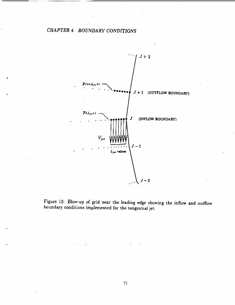
CHAPTER 4. BOUNDARY CONDITIONS
"'" J+2
,.r+,.L,,+, .---_.. +" " " eeeee I (OUTFLOW BOUNDARY)
PJ,L_.+I ---_
• " " " " " TIIIII
Vj_t
.......... 3-1
Ljo,values
3 (INFLOW BOUNDARY)
J-2
Figure 12: Blow-up of grid near the leading edge showing the inflow and outflow
boundary conditions implemented for the tangential jet.
71

Chapter 5
Discussion of Results
5.1 Preliminary Comments
This chapter presents the results obtained for a variety of cases involving computa-
tions of a rotor alone and wing/rotor interaction. Results for the rotor alone serve
not only to validate the current numerical model, but also to highlight some of its
limitations. Computations have been performed for a uniformly-loaded rotor with
no swirl, where a constant pressure rise across the disk is specified. Results for a
non-uniformly-loaded rotor with swirl are also presented, where the rotor is modeled
using the blade element/momentum theory described in Chapter 4. Computed re-
sults of wing/rotor interaction are presented for both of the above rotor models. This
highlights the effects on wing download of swirl in the rotor flowfield. Finally, the
effect on download of tangential blowing at the wing leading edge is shown.
Most of the visualization of the grids and solutions during the course of this
work, and many of the figures in this report, have been generated using the computer
graphics program known as PLOT3D [71,72]. Developed by Buning at NASA Ames
Research Center, PLOT3D is a powerful interactive graphics tool capable of calcu-
lating and displaying a considerable number of different flowfield functions including
pressure, Mach number, velocity vectors, and particle traces.
72

CHAPTER 5. DISCUSSION OF RESULTS
5.2 Rotor Alone
Accurate definition of the wing using stacked O-grids, as discussed in Chapter 3,
results in a Cartesian-like grid representation for the rotor (refer, for example, to
Fig. 10). Therefore, to provide a test, for the rotor alone, which is representative of
the rotor model in the wing/rotor interaction computations, a Cartesian grid is used.
The outer boundaries of the Cartesian grid extend five rotor radii from the rotor disk
axis of rotation in the horizontal and vertical directions. The grid has dimensions
of 47x47x47 with most of the grid points clustered in the region of the rotor disk.
On each of the two principal axes on the rotor disk are defined 26 points along the
rotor diameter. The grid spacing stretches from a minimum of 0.01R at the plane
of the rotor to 0.4R at the top and bottom boundaries. The grid point distribution,
though not identical to, is representative of that used in the wing/rotor computations
discussed later. Figure 13 shows both a vertical cut and a horizontal cut through the
center of the grid. The side view shows the clustering of points near the edge of the
rotor. The location of the rotor disk is highlighted in the top view. All rotor alone
computations assume that the flowfield is laminar throughout.
5.2.1 Rotor with Uniform Loading and No Swirl
Figures 14-16 show typical results for a uniformly-loaded rotor disk without swirl. As
mentioned in Section 4.3, the presence and influence of the nacelle and the rotor hub
have been neglected. For the results discussed here, a pressure rise Ap/po_ = 0.0119
is specified across the rotor. Since Ap is constant, it also represents the rotor thrust
loading T/A. From the definition of the rotor thrust coefficient CT (see Eq. 57), and
assuming a rotor tip Mach number Mtip = 0.72 (typical of the experimental rotor tests
described in Refs. [9,10]) and freestream conditions for density and speed of sound
(reasonable assumption for the relatively low induced flow speed of the tilt rotor in
hover), then for Ap/poo = 0.0119, the rotor thrust coefficient is 0.0164. A value of
CT = 0.0164 is specified for many of the computations discussed in this chapter as
it represents a typical thrust loading for the V-22 in hover. Also, experimental data
exists at or near this value of CT.
73

CHAPTER 5. DISCUSSION OF RESULTS
Figure 14 shows the contours of static pressure normalized by freestream pressure
p/p_ around and through the rotor in a vertical plane through the rotor diameter.
The cross-section of the rotor, whose dimensions have been normalized with respect to
rotor radius, has been superimposed on the plot. Far above the rotor, the pressure is
freestream ambient. As the rotor disk is approached from above, the flow accelerates
and the static pressure drops. Note the pressure jump across the rotor disk. The
flowfield is driven solely by this pressure rise. Below the rotor, the flow recovers its
freestream value as the induced rotor flow attains a constant velocity. The contours
of velocity magnitude (normalized by the freestream speed of sound) presented in
Fig. 15 clearly show the flow being accelerated from a quiescent state above the
rotor, drawn into the rotor, and accelerated to some maximum value below the rotor.
This behavior is expected from simple momentum theory (see, for example, Ref. [18]).
From momentum theory, the ideal induced velocity at the rotor disk is given by
Vh = _/2--_ (62)
Note that by substituting Eq. 57 into Eq. 62, the ideal induced velocity can also be
expressed in terms of the rotor thrust coefficient in hover, i.e.
Vh = 9tR _ (63)
As previously mentioned, for Ap uniform on the rotor disk, T/A = Ap. From Eq. 62,
then, with Ap/p_ = 0.0119, and assuming freestream density, the ideal induced hover
velocity normalized by the freestream speed of sound Vh is 0.06519. From simple
momentum theory, the velocity induced in the far wake is twice that at the rotor
disk; i.e. for this case, 2Vh = 0.1304. This compares well with the computed value of
0.133. From Fig. 15 it can be seen that the flow into the rotor is fairly uniform except
for a slight variation of induced velocities in the rotor plane along the diameter. The
average flow velocity through the rotor disk appears to be somewhat higher than the
ideal value of Vh. Also, the rotor wake contraction to 71% of the rotor diameter,
anticipated from momentum theory, is not fully attained in the computation, as is
shown more clearly in the next section. This is due to the fact that there is an
insufficient number of grid points, particularly on the outer portion of the rotor disk
74
CHAPTER 5. DISCUSSION OF RESULTS
and wake, to compute more accurately the edge of the wake and its contraction. This
lack of resolution in the wake also affects the computed flowfield at and above the
rotor disk. Velocity contours in the wake (see Fig. 15) show that the flow velocities
are fairlY constant in the far wake along its width. Some wake dissipation is evident
as the flow approaches the exit boundary -- i.e. the flow gradually decelerates and
the wake widens slightly. This is due to a combination of numerical and artificial
diffusion. Numerical dissipation increases with increasing grid cell size. The stretched
grid spacing below the rotor (refer to Fig. 13), therefore, contributes to the diffusion
of the wake. The Cartesian grid makes it difficult to resolve the axisymmetric rotor
flowfield with uniform accuracy for all azimuths of the rotor disk. This contributes
to the slight non-uniformity on the rotor disk.
Figure 16 shows the velocity vectors through the rotor projected onto the vertical
plane. Note the changing flow angles as the rotor disk is approached from above. The
flow accelerations described above are clearly indicated by the changing lengths of
the velocity vectors. The effect of numerical diffusion can be seen at the edge of the
rotor slipstream. Experimental data shown later in this chapter indicates that the
edge of the actual slipstream is considerably more distinct and the velocity gradient
significantly greater. A finer mesh would be required to better resolve the shear layer
formed between the inner and outer flowfields.
5.2.2 Rotor with Non-Uniform Loading and Swirl
This section describes the results obtained for a rotor imparting non-uniform radial
distributions of pressure rise across the disk and of swirl velocity. The rotor simulated
is the V-22 rotor operating at a thrust coefficient of 0.0164 and a rotor blade tip Mach
number Mtip = 0.72. The blade chord and twist distributions, required for the blade
element analysis, are taken from Ref. [10]. The blade geometry is extrapolated inboard
from the hub location (at r/R _ .09) to the rotor centerline (r/R = 0), as can be
seen in Fig. 17. Similar to the uniformly-loaded rotor model discussed in the previous
section, the presence and influence of the nacelle and the rotor hub are neglected.
The rotor disk is divided into annular elemental areas of equal width dr. Since cir-
cumferential variations do not exist for a rotor alone (modeled as an actuator disk) in
75

CHAPTER 5. DISCUSSION OF RESULTS
hover, the annuli are not subdivided azimuthally as is done for the wing/rotor inter-
action computations discussed later in this chapter. For the computations discussed
here, the rotor disk is subdivided into l0 annular rings.
The only modification made here, to the rotor model described in Chapter 4, is
the imposing of a limit on the magnitude of swirl velocity allowed at the most inboard
annulus. It was found that not constraining the swirl often yielded unstable solutions
because of the far-from-optimum flow angles in the blade root region where the rota-
tional speed approaches zero: This resuIted in the computation of oscillatory positive
and negative swirl velocities. The swirl at the inner-most annulus is, therefore, con-
strained to be positive and less than 0.06 when normalized by the freestream speed
of sound. It was found that this did not significantly affect the converged solution
because the computed swirl velocities were always somewhat less than this value.
Figure 18 shows the computed radial distributions of blade loading (local blade
lift and drag coefficients, Cl and Cd, respectively) and local blade angle of attack
a for a non-uniformly-loaded rotor with CT = 0.0164. Figure 19 shows the radial
distributions of axial velocity V, and swirl velocity V,, normalized by the freestream
speed of sound, computed at the rotor disk (i.e. at the horizontal layer L of rotor grid
points -- see Chapter 4). Experimental measurements of rotor blade loading and
local flow angles and velocities in the rotor disk, or immediately below it, are difficult
to make, and none are available for the V-22 rotor. Beyond the inner region of the
rotor, say for r/R > 0.2, the computed results shown in Figs. 18 and 19 are probably
fairly representative of the actual loads and velocities. Referring to Fig. 18, note
that proceeding radially outwards, the angle of attack decreases and Cl tracks this
behavior. The dip in the Cl curve and the spike in Cd near r/R = 0.25 is due to the
local angle of incidence exceeding the stall angle, resulting in a local loss of lift and a
large increase in drag. Due to the reduced axial velocities at the outer edge of the rotor
disk, a slight increase in a is predicted at the blade tip. Being well below the stall
angle, the local lift coefficient also increases proportionately. The increase in drag,
however, is due not to the change in a, but to compressibility effects in the tip region
(remember that Mt_p = 0.72). Compressibility drag is introduced through the table
look-up described in Section 4.3. Due to the absence of the hub, axial flow is induced
75

CHAPTER 5. DISCUSSION OF RESULTS
in the inner region of the rotor disk. The blade twist at the root is insufficient to
accommodate the relatively high axial velocity (relative to the rotational component
of velocity) as evidenced in the rapid drop to a negative angle of incidence. This causes
Ct to become negative, and in turn, would yield a negative swirl velocity if Vt hadn't,
rather arbitrarily, been set to zero for reasons mentioned previously. Outboard of the
hub region, however, as can be seen in Fig. 19, the swirl, which is generally greatest in
the inboard region of the rotor disk, decreases as r/R increases. The increase in swirl
at the tip is due to the local increase in lift and drag coefficients, described above. The
increase in the induced axial velocity V_ from the rotor center outboard, as evidenced
in Fig. 19, is expected for a CT = 0.0164. The effect of CT on local induced velocities
is discussed in more detail below, where comparisons with experiment are made. The
relative magnitudes of swirl velocity with respect to axial velocity are representative
of the actual rotor flowfield. From momentum theory analysis (see Ref. [18]), it is
known that swirl velocities are generally considerably smaller in magnitude than are
axial velocities except in the inboard region of the rotor disk where their magnitudes
may be similar.
Figures 20 and 21 show the contours of normalized pressure (p/poo) and of nor-
malized velocities (IVI/aoo), respectively, in a vertical plane through the center of the
rotor disk. Comparing these figures with Figs. 14 and 15, the non-uniform rotor disk
loading is clearly seen to cause a significant flow non-uniformity radially, particularly
near the rotor disk. Figure 20 actually shows a small amount of negative loading
produced near the center of the rotor disk. This is a result of the far-from-optimum
flow angle that the rotor blade sees in this region. As mentioned previously, the rotor
blades are assumed to extend all the way to the rotor center, thereby neglecting the
presence and influence of the rotor hub. The maximum computed induced veloc-
ity in the rotor wake is 0.1300 which is near identical to the ideal induced velocity
2Vh = 0.1304 derived from Eq. 63, again providing confidence that the current rotor
model is valid. The velocity contours show that the wake exits the lower boundary as
expected. The gradual spreading of the contour lines, however, again demonstrates
the effect of numerical dissipation.
77

CHAPTER 5. DISCUSSION OF RESULTS
As mentioned in Chapter 4, the rotor imparts a rotational or swirl velocity com-
ponent to the flowfield. Above the rotor, the swirl is zero. Below the rotor, the rota-
tional motion is maintained in the wake downstream of the rotor. Figures 22 and 23
show the effect of the swirl computed by the non-uniformly-loaded rotor model with
CT = 0.0164. Figure 22 shows views of the velocity vectors projected onto two dif-
ferent horizontal planes: (i) immediately above the rotor, and (ii) immediately below
the rotor. The extent of the rotor disk is shown on these plots. The view labeled
"immediately above rotor" is actually a view looking down at the horizontal plane
that contains the L + 1 layer of rotor grid points (see Chapter 4). As expected, the
swirl is effectively non-existent. The view labelled "immediately below rotor" shows
the results at the "L" layer of rotor grid points. The swirl velocity, computed using
the blade element/momentum theory analysis described in Chapter 4, is specified
at these points. Figure 22, then, serves to confirm that the discontinuous nature of
the swirl motion is being computed. Figure 23 shows two views of particle traces
which demonstrate the effect, on the flowfield downstream of the rotor, of the swirl
imparted at the rotor disk. Particles are seeded into the flowfield at every grid point
on the rotor centerline immediately above the rotor. The side view clearly shows that
the rotational flowfield motion imposed at the rotor is communicated to the flowfield
beneath the rotor, as expected. The top view also Shows the rotation in the flow-
field. The wake contraction is clearly evidenced. The wake contracts very quickly
beneath the rotor disk to a minimum diameter of about 84% of the rotor diameter.
As mentioned in the previous section, the wake contraction, from simple momentum
theory, is 71% of the rotor diameter. The azimuthal non-uniformity of the computed
wake seen in the top view of Fig. 23, and the discrepancies between the computed
and the theoretical wake contraction are due, in large part, to the difficulty that the
Cartesian grid is experiencing in computing more accurately the cylindrical-shaped
flowfield. Along lines that are forty-five degrees to the principal axes of the grid in
the horizontal plane, the mesh resolution of the outer edge of the rotor disk and its
wake is at its worst. This can be more clearly visualized by referring back to Fig. 13
which shows the top view of the grid. Use of a finer mesh and a cylindrically-shaped
one would help to further improve the solution.
78

CHAPTER 5. DISCUSSION OF RESULTS
The comparisons discussed below are made with experimental results obtained for
a 0.658-scale V-22 rotor in hover (see Refs. [2,9]). The computed results shown are for
a case where the rotor is alone, not influenced by a plane of symmetry. Figure 24 is
a plot of the induced velocity as a function of radial location. The induced Velocities
are those in a horizontal plane below the rotor at a vertical location that corresponds
to the position of the wing of the V-22 tilt rotor configuration. The velocities are
normalized here by the ideal induced velocity at the rotor disk in hover Vh defined in
Eq. 63. The results for two different thrust coefficients are presented: CT = 0.0164
and CT = 0.0051. The experimental tests show that the radial distribution of in-
duced velocity is sensitive to the thrust coefficient. For the twist distribution of the
V-22 rotor blades, as CT and the corresponding blade pitch angle increase, the lo-
cal aerodynamic blade loading becomes greater in the outboard region of the rotor
thereby inducing greater velocities in the outer portion of the wake. At low thrust
coefficients, the inboard region is more highly loaded. As can be seen from Fig. 24,
these trends with CT are predicted numerically although the actual computed veloc-
ities differ somewhat from the experimental measurements. The computed velocities
extend to the rotor centerline because, as previously mentioned, the nacelle has not
been modeled. The diffusion of the slipstream shear layer, discussed earlier, prevents
a more accurate prediction of induced velocities.
Figure 25 shows a comparison of rotor figure of merit FM (defined in Eq. 58 of
Chapter 4) between experimental results taken from Ref. [2] and computational re-
sults. As the thrust coefficient decreases, the disk loading decreases, thereby reducing
the induced power relative to the profile power. The figure of merit, therefore, de-
creases as CT decreases. Due to blade stall at high CT, the profile losses increase and
the figure of merit again begins to drop. The experimental figure of merit is predicted
quite well by the numerical computation, over a range of rotor thrust coefficients.
These results show that, despite the inaccuracies associated with not modeling the
hub and nacelle or the discrete vorticity (rotor tip vortices) in the wake, and with less
than optimum grid resolution due to limited computer resources, the current actuator
disk model of the rotor simulates the expected overall flowfield behavior fairly well.
79

CHAPTER 5. DISCUSSION OF RESULTS
5.3 Wing/Rotor Interaction
The results discussed in this section are from computations of wing/rotor interaction
in hover. To verify, at least qualitatively, that the method developed here yields solu-
tions that are intuitively correct, the first computations described are for a uniformly-
loaded rotor with no swirl. These results are followed by wing/rotor computations
where the rotor model described in Section 4.3 is used. The non-uniform loading and
swirl calculated by this model is a far better simulation of the actual rotor flowfield.
Comparisons are made with experimental measurements of wing pressures and down-
load. Also, comparisons of the computational results are made between the uniform
and the non-uniform with swirl rotor models. This clearly shows the effect of swirl
on the wing. Finally, computations of tangential jet blowing are described.
The geometry of the V-22 wing/rotor configuration is used as a basis for the
numerical model. There are, however, notable differences. As mentioned in previous
chapters, to simplify the grid generation, the fuselage, tail, nacelle, and rotor hub are
not modeled. The six degrees of forward sweep of the V-22 wing is also not modeled.
The wing and rotor are assumed in this study to be coplanar when they are actually
angled 6 ° with respect to each other. The V-22 possesses 3.5 ° of wing dihedral and
2.5 ° of lateral nacelle cant. The nacelle is not modeled, and the center of the rotor
is placed above the wing tip (not displaced outboard a distance equal to the nacelle
half-width as in the actual configuration). The rotor radius of the numerical model is
therefore reduced by the nacelle half-width to keep the extent of the rotor disk which
lies above the wing essentially the same for both the actual and the computational
configurations. The rotor disk of the numerical model was centered above the wing
tip in anticipation of future comparison of results with those obtained from a NASA
Ames OARF (Outdoor Aerodynamic Research Facility) test of a simplified 0.16-scale
wing/rotor configuration (which has no nacelle). Normalized by the wing chord, the
effective rotor radius is 1.98, the wing semi-span is 2.45, and the rotor height above
the wing is 1.10 (an average of the varying height of the V-22 rotor disk above the
wing). The wing is of constant chord with an airfoil section having a thickness/chord
ratio of 0.23. Unless noted otherwise, the results reported here are all with the flap
8O

CHAPTER 5. DISCUSSION OF RESULTS
deflected to 670 . The rotor axis of rotation is, as mentioned above, located at the
wing tip, and is 55% of the wing chord aft of the wing leading edge. A rotor blade
tip Mach number of 0.72 is assumed for all the calculations. Also, except where
noted otherwise, the rotor thrust coefficient is 0.0164. The Reynolds number for the
calculations described here is based on wing chord and ideal hover induced velocity.
For CT = 0.0164, the Reynolds number is 2.6x10⁶. No attempt is made to model the
turbulence imparted by the rotor into the rotor slipstream.
5.3.1 Rotor with Uniform Loading and No Swirl
Similar to the rotor alone computations described in Section 5.2.1, a uniform rotor disk
loading of Ap/poo = 0.0119 is specified. As previously mentioned, with Mtip = 0.72,
this corresponds to an effective thrust coefficient of 0.0164. Figures 26 - 34 show the
results obtained with the uniformly-loaded rotor.
Figure 26 is a perspective view of the computed velocity vectors on the near-
vertical computational grid plane that runs through the wing mid-chord line. The
viewpoint is outboard of the wing tip and ahead of and above the wing. Flow accel-
eration through the rotor disk is clearly evidenced as is the flow stagnation on the
wing upper surface. Close examination of the region below the wing tip shows the
existence of a standing vortex. A recirculation flow pattern -- the fountain flow --
is also visible in the wing root region adjacent to the plane of symmetry.
Figures 27, 28, and 29 show the velocity vectors, the velocity magnitude (normal-
ized by a_o), and the pressure (normalized by poo), respectively, in a vertical plane
that runs spanwise through the wing mid-chord. From Fig. 27, it can be seen that the
flow is near-vertical beneath much of the rotor. The flow is spanwise outboard in the
wing tip region both on the upper surface and the lower surface. As the wing surface
is approached from above, the flow stagnates at about the three-quarter semi-span
location and is re-directed spanwise inboard and outboard. The velocity vectors at
the inboard region of the wing indicate that at this mid-chord location, the fountain
extends less than 0.5c above the wing. As is shown in the next section, a portion of
the computed fountain reaches a height of one chord above the wing, but at an x/c
location further forward on the wing. The blockage effect of the wing on the flowfield
81

CHAPTER 5. DISCUSSION OF RESULTS
is clearly seen in Figs. 28 and 29 by comparing the flow above the wing with the
flow outboard of the wing. The presence of the wing tends to reduce the velocity
and increase the pressure in that portion of the rotor flowfield that lies above the
wing. The small discontinuities at 2y/b = 2.45 are due to an insufficient number of
2-D grid planes in the Wing tip region to adequately resolve the flow. Convergence of
the solution near the singular line that emanates spanwise from the wing tip (refer
to Chapter 3) is slow, and a small residual effect is seen in the velocity magnitude
contours.
Figures 30, 31, and 32 are views of the flowfield at a typical spanwise station,
2y/b = 0.7. The location of the rotor disk is highlighted in the figures. Figure 30
shows the velocity vectors projected onto the vertical plane. Because there is no swirl,
the flow through the rotor is near-symmetric about a vertical line running through
the center of the rotor. These results are compared later with those obtained with
the rotor swirl modeled. It will be seen that swirl introduces considerable asymmetry
to the flowfield. From Fig. 30, it can be seen that the flow impinges on the wing
surface and is re-directed fore and aft, accelerating around the leading edge and the
knee (junction of main foil and flap) of the flap. In the wake beneath the wing the
computation predicts the formation of two side-by side vortices, one shed from the
leading edge and the other shed from the trailing edge. Whether this represents the
real physical flowfield or not must be determined from future experimental measure-
ments and flow visualization. The influence of the wing on the rotor flowfield is clearly
evidenced in the velocity and pressure contour plots of Figs. 31 and 32, respectively.
The presence of the wing reduces the velocity and increases the pressure of that por-
tion of the rotor flowfield which lies above the wing. As expected, as the wing surface
is approached from above,_ : the=_flow_:_._continues to decelerate: : and the pressure continues
to increase. Away from the wing, near the edges of the rotor wake, the flowfield
remains essentially unaffected by the wing. The influence of the wing on the rotor
flowfield can be better appreciated by comparing with the results of the rotor alone,
Figs. 14, 15, and 16. The oscillations in the pressure immediately below the rotor
could probably be eliminated by further grid refinement.
Convergence of the numerical solution is determined by the attainment of a steady
82

CHAPTER 5. DISCUSSION OF RESULTS
. r
value of the mean download/thrust ratio, i.e. when the time-averaged download/thrust
DL/T is constant. Actually, the computation was generally stopped when the percent
change in time-averaged download/thrust between cycles was less than 0.2. "Pseudo
2-D" computations of an airfoil/actuator line configuration were performed during
the course of this work to aid in the development of the numerical method, the
grid, and the boundary conditions. These two-dimensional computations showed a
much greater degree of unsteadiness in the flowfield than is observed in the three-
dimensional results. This is due to the alternate shedding of vorticity from the
leading and trailing edges that is computed in 2-D but not in 3-D. In two dimen-
sions, it was observed that these vortices propagate downstream in a vortex street
typical of bluff body flows. Results from these 2-D calculations were reported by
the author in Ref. [73]. This unsteady wake behavior has also been computed in
the two-dimensional analyses undertaken by Raghavan et al. [16] and Stremel [17]
for low Reynolds number laminar flows. As mentioned previously, the converged
three-dimensional solution shows two standing vortices, of opposite sense of rotation,
side-by-side beneath the wing. This difference in unsteadiness of the wing wakes be-
tween the 2-D and 3-D computations is manifested in a plot of instantaneous DL/T
versus non-dimensional time t aoo/c. Figure 33 shows the behavior of download/thrust
with time as the computation proceeds_ starting with an initially-quiescent flowfield
and an impulsive start of the rotor pressure rise. Both the 2-D and 3-D compu-
tations show high frequency start-up transients which damp out rapidly. There is
an overshoot of DL/T before a near-constant mean value is reached. Computations
are generally continued a few more cycles than shown here, until the mean value
of DL/T varies less than about 0.2% between cycles. The 2-D computation takes
longer to settle to a constant mean value and the amplitude of periodic oscillation
of download/thrust is muchgreater than in the three-dimensional computation. As
previously mentioned, the differences in the unsteadiness are due primarily to the
differences in the computed vortical flow in the wing wake. Lack of experimental
data for, and flow visualization of, this type of flowfield make it difficult to determine
the validity of the wake solutions. One would expect, however, less flow unsteadi-
ness in 3-D due to the relaxing effect of a finite wing on the flowfield, but to what
83

CHAPTER 5. DISCUSSION OF RESULTS
extent is unknown. The observed differences in the computed wakes are probably
due to a combination of flow physics, an insufficient number of grid points to resolve
all the complicated flow features, numerical and artificial dissipation, and simplifica-
tions made in the thin-layer Navier-Stokes equations and in the turbulence model.
Suggestions for improvements to the current model are discussed in Chapter 6.
Figure 34 is the computed oil flow pattern on the wing upper surface, viewed
form the rear beyond the wing tip. The flow stagnates in the three-quarter semi-span
region of the wing, and from this location the flow is re-directed spanwise inboard
and spanwise outboard. The flow symmetry at the wing centerline is evidenced in
the wing root region. The flow is primarily chordwise in the outer region of the wing
and becomes more spanwise inboard, as expected. At the wing centerline the flow is
re-directed chordwise fore and aft as indicated by the oll traces, and also vertically
upwards to form the recirculation fountain. Note that the flow proceeds smoothly
over the flap with no sign of separation.
5.3.2 Rotor with Non-Uniform Loading and Swirl
The results discussed below are for wing/rotor interaction where the non-uniform
loading and swirl imparted by the rotor is modeled, using the method described in
Chapter 4. The rotor model is the same as that used to obtain the rotor alone results of
Section 5.2.2. The computations discussed below are for a case where the rotor thrust
coefficient is 0.0164 and the rotor tip Mach number is 0.72. When comparisons with
experiment are made, the data is taken from either the OARF test (see Ref. [9]) or the
40- by 80-Foot Wind Tunnel test (see Ref. [10]) conducted at NASA Ames Research
Center on a 0.658-scale V-22 rotor and wing used to study wing/rotor interactions
in hover: Figure 35, taken from Ref. [10], is a schematic of the 40- by 80-Foot Wind
Tunnel model installation showing the wing, rotor, image plane, and model support
structures.
Many of the flow features that were described in the previous section, com-
puted using a uniformly-loaded rotor disk with no swirl, also occur when the more-
representative model of the rotor is used. The fountain flow at the plane of symmetry,
84

CHAPTER 5. DISCUSSION OF RESULTS
the chordwise flow on the outer region of the wing surface and the spanwise flow fur-
ther inboard, the standing vortex beneath the wing tip, and the flow accelerations
through the rotor and around the leading and trailing edges are all observed with
the non-uniformly-loaded rotor disk model. The results shown in this section serve
to highlight the flow features that either do not appear or are somewhat different if
the non-uniform loading and swirl are neglected.
The rotor's introduction of swirl into the flowfield is clearly shown in Fig. 36.
Figure 36(a) shows the velocity vectors projected onto a horizontal plane immediately
above the rotor. The flow is generally radial inwards towards the center of the rotor.
In the region above the wing tip, it appears that the presence of the wing tip causes
a small amount of radial-outwards movement of the flow. Figure 36(b) shows the
velocity vectors in a horizontal plane immediately below the rotor. The increasing
tangential (swirl) component of the vectors, as one moves from the edge of the rotor
disk towards the center of the rotor, represents the increasing magnitude of the swirl,
similar to that observed previously for the rotor alone in Figs. 19 and 22.
The fountain flow is clearly seen in Figure 37 which shows the instantaneous
particle traces in a near-vertical spanwise plane in the region of the wing root. Note
that the particles are drawn into the rotor from above, and as the wing surface is
approached, the flow is re-directed spanwise inboard and outboard. Similar views
can also be seen when rotor swirl is not modeled. It seems, then, that swirl has
very little effect on the strength or location of the fountain. The fountain reaches
a maximum height of about 1 chord above the wing surface at a chordwise location
between the mid-chord and the leading edge -- i.e. in the vicinity of the maximum
thickness location of the airfoil section which lies at x/c _ 0.30. Limited experimental
flow visualization was obtained from the OARF test of the 0.658-scale model of the
V-22 wing, rotor, and wing/fuselage fairing [9]. Tufts on the image plane and smoke
released near the plane of symmetry indicate that the actual recirculation pattern
(fountain) is somewhat larger than that computed, extending about two chords above
the wing. This difference can at least partially be explained by the presence of the
large wing/fuselage fairing in the experimental model which tends to increase the
portion of the flow that is re-directed upwards.
85

CHAPTER 5. DISCUSSION OF RESULTS
Figure 38 is a perspective view of the computed oil flow pattern on the wing
upper surface, as seen looking from the rear towards the flap from beyond the wing
tip. The numerical results show the transition of primarily two-dimensional flow to
three-dimensional flow towards the wing root. Flow visualization from the OARF test
indicates that the 2-D behavior extends to the wing tip, whereas the computation
yields considerable spanwise flow over the tip. This discrepancy may be due, at least
in part, to the flow straightening effects of the nacelle and large, flat model support
structure used in the test (refer to Fig. 35). In the three-quarter semi-span region,
where the flow is primarily chordwise, the flow separates on the flap due to the adverse
pressure gradient, and a region of flow reversal can be seen on the upper surface of
the flap in Fig. 38. This flow separation on the flap does not occur when the rotor-
induced swirl is not modeled. As seen previously in Fig. 34, the flow is smooth and
unseparated over the entire length of the flap surface when the rotor is modeled as a
uniformly-loaded disk with no swirl.
In the following discussions, reference is made to specific spanwise locations. As
an aid to visualizing these locations relative to the extent of the rotor disk, reference
should be made to Fig. 39. The edge of the rotor disk reaches a minimum spanwise
value of 2y/b = 0.19, or, relative to the wing chord, y/c = 0.47. Figure 40 is a
typical view of the projection of velocity vectors onto a vertical, chordwise plane
that lies well within the rotor slipstream -- here corresponding to 2y/b = 0.7. Note
the discontinuity in velocity direction at the rotor disk due to the swirl imposed
there. The leading edge-to-trailing edge bias in the flowfield is also due to rotor
swirl. In contrast, for a case where the swirl is zero, Fig. 30 of the previous section
shows a flowfield that is much more symmetric about the mid-chord with no velocity
discontinuity at the rotor disk.
Figure 41 shows a comparison of wing surface pressures at the same spanwise
location as above, i.e. 2y/b = 0.7, computed using the two different rotor models.
The pressures are relative to freestream ambient pressure, normalized by rotor thrust
loading, i.e. (p - p_)/(T/A). Due to the unsteadiness in the wake that causes small
amplitude fluctuations in download, these pressures are time-averaged over one period
of oscillation of DL/T. Also, x/c is the distance along the chord from the leading
86

CHAPTER 5. DISCUSSION OF RESULTS"
O
|-i
edge, normalized by the undeflected flap wing chord. The computed base pressure
(pressure along the lower surface) is uniform, typical of bluff body flows, and is near-
identical for both cases -- i.e. it appears to be quite independent of swirl. The
upper surface, on the other hand, sees pressure distributions that differ considerably
depending on whether the swirl is modeled or not. The pressure for the case with no
swirl is somewhat more uniform and more symmetrical about the mid-chord. The flow
stagnates in the mid-chord region. With swirl, however, the flow stagnates further
forward, closer to the leading edge. Because of the swirl-induced bias in the flowfield,
the flap sees an onset flow that is at a considerably higher angle of attack. This causes
a greater local flow acceleration and reduced pressure at the knee of the flap, relative
to the case where there is no rotor swirl. The flow experiences, then, a much larger
adverse pressure gradient as it approaches the trailing edge. This contributes to the
flow separation on the flap upper surface observed in Fig. 38 that does not exist in
the absence of swirl (see Fig. 34).
Figure 42(a) - (e) show the wing surface pressure distributions at five different
spanwise stations. The computational data has been linearly interpolated to obtain
the pressures at the desired spanwise locations. The experimental data has been taken
from the "normal" pressure coefficient distributions of Ref. [10]. As can be seen from
the plots of Fig. 42, there is an insufficient number of experimental data points to
resolve the negative pressure peaks at the wing leading edge. The comparison of com-
putational results with the experimental measurements is generally more favorable in
the mid-semispan region of the wing than at the root or the tip. Outside of the rotor
wake, at 2y/b = 0.145 (see Fig. 42(a)), the upper surface pressures compare very well
while the computed base pressure is somewhat greater than the experimental values.
This seems to indicate that the actual wake contains shed vortices whose strengths
are a little greater than those computed. The negative pressure peak at the knee of
the flap is very well-predicted. These same comments apply to Figs. 42(b) and (c), at
2y/b = 0.332 and 2y/b = 0.518, respectively, except that the upper surface pressures
are over-predicted. At 2y/b = 0.705 (see Fig. 42(d)), both the upper and lower surface
pressures are very well predicted. That the upper surface pressures compare so well
87

CHAPTER 5. DISCUSSION OF RESULTS
at 2y/b = 0.705, but not as well further inboard on the wing, is due to differences be-
tween the computed and the actual rotor-induced velocities. As discussed earlier for
the rotor alone results (refer to Section 5.2.2), these discrepancies are due primarily to
an insufficient number, and less than optimum distribution of, grid points required to
adequately resolve the radial distribution of rotor-induced flow. This contributes to
inaccuracies in resolution of the rotor flowfield and to unwanted numerical dissipation
which causes diffusion of the edge of the rotor slipstream.
Figure 42(e) shows the comparison of pressures near the wing tip, at 2y/b = 0.891.
The upper surface pressure is generally under-predicted as a result of the spanwise-
outboard flow computed in the tip region (see, for example, Fig. 38) relative to the
primarily chordwise flow seen experimentally. This also explains the reduced nega-
tive pressure peak over the flap, compared with experiment. Spanwise flow towards
the wing tip was also computed in the previous section where a uniform pressure
rise was specified across the rotor. This difference between the computed and the
experimental flowfields, as stated previously, can be partially attributed to the flow
straightening effects of the nacelle and model support structure of the experimental
set-up. Also, the fact that the rotor centerline is actually about 13%R outboard of
the wing tip of the experimental model, encourages 2-D flow near the wing tip. As
mentioned previously, anticipating future comparisons of results with on,going tests
of a 0.16-scale simplified tilt rotor configuration at NASA Ames, the center of the
rotor disk for the computation is above the wing tip -- not displaced beyond the
wing tip. The offset rotor centerline reduces the affect on the wing of the poor qual-
ity, low dynamic pressure flow that is generated at the inboard rotor region due to
the far-from-optimum blade angles and blade thickness, and rotor hub interference.
Thus, the flowfield in the wing tip region of the experimental model probably has
a greater axial component which results in the greater chordwise flow. It should be
remembered that the computed flow velocities and angles in the inner region of the
rotor are not accurate representations of the actual flowfield. This contributes to
the discrepancies in wing surface pressures in the wing tip region between the com-
putational and the experimental results. The computed lower surface pressures at
2y/b = 0.891 are somewhat less than the measured values. This is also probably due
88

CHAPTER 5. DISCUSSION OF RESULTS
to the increased spanwise flow predicted for the tip region. This causes a stronger tip
vortex to be formed beneath the wing tip (see the standing vortex in Fig. 26) which
induces a greater velocity at the lower wing surface reducing the base pressure.
Bearing in mind the differences in configuration between the computational and
experimental models, the comparison of wing surface pressures is generally quite good.
Figure 43 compares the computed and measured time-averaged download/thrust
per unit span normalized by the total time-averaged download/thrust. The computed
distribution generally follows the shape of the experimental distribution. The edge
of the computed rotor wake is diffused over several grid points, thus contributing
to the more gradual download gradient in the region 0.2 < 2y/b < 0.5. Greater grid
point density, particularly in the region of the edge of the rotor slipstream, would be
required to compute the spanwise download distribution more accurately. There is
insufficient experimental data to observe the expected local increase in download at
the wing root. The local increase in DL/T, predicted by the computation, is produced
by the change in momentum due to the flow turning away from the surface in the
recirculating fountain near the wing centerline.
The computed time-averaged download/thrust is 0.113 for the specified rotor
thrust coefficient CT = 0.0164. This is somewhat higher than that measured in
the 0.658-scale model tests at NASA Ames, for the same thrust loading. For flaps
deflected to 67 °, and at a rotor tip Mach number approximately 0.70, a DL/T of
0.093 was measured in the OARF test [9] and a DL/T = 0.078 was measured in the
40- by 80-Foot Wind Tunnel test [10]. The latter test was performed with the na-
celle set at an angle of 85 degrees with respect to the wing chord line (tilted forward
slightly) -- not at 90 ° which is typical for the V-22 aircraft in hover. Felker [11]
estimates that the download is reduced by about one percent of rotor thrust for 10 ° of
forward nacelle tilt. Using this as a guideline to estimate the download with the na-
celle set at 90 ° gives DL/T = 0.083. The configurations for the two NASA tests were
essentially the same except that the OARF model included a fuselage fairing, and the
rotor for the 40- by 80-Foot Wind Tunnel test was slightly modified at the blade root.
The presence of the fuselage fairing in the OARF test increases the download/thrust,
but to what extent is unknown. It is interesting to note that, extrapolating flight test
89

CHAPTER 5. DISCUSSION OF RESULTS
data presented in Ref. [2], DL/T for the XV-15 aircraft at flaps 67 ° is approximately
0.10. The figure of merit, calculated from the current computation, is 0.746. This
compares with 0.755 computed for the rotor alone (see Fig. 25). The tendency for
the hover efficiency to drop when the rotor is in the presence of the wing (in the tilt
rotor configuration) was also observed experimentally at the OARF. The measured
figure of merit was reduced by about 2%, and as discussed in Ref. [2], is due to the
negative impact of the re-ingested flow from the fountain.
Even accounting for uncertainties associated with the experimental measurement
of download/thrust, the computed DL/T is somewhat greater than expected. This
discrepancy can be attributed to several factors. The rotor plane and wing are not
coplanar in the experimental models, as discussed earlier in Section 5.3. This is
expected to contribute to the lower measured download/thrust, relative to the com-
puted value. As discussed earlier, the lack of sufficient number of grid points and
the less than optimum grid point distribution, particularly near the edge of the rotor
slipstream, contribute to inaccuracies in the computed solution. Early computations
using a grid of size 53x42x46 -- a size selected to permit job execution in the 4 mega-
word memory queue of the CRAY Y-MP -- yielded a DL/T = 0.185. The present
mesh (73x46x70) is the largest single zone grid that could be handled by the Cray
Y-MP (whose current memory limit is 8 megawords per job). Despite the difficulty in
performing grid sensitivity studies on problems of this magnitude, it is obvious that
further work would be required to determine to what extent the number of grid points
affects the solution. Another source of uncertainty in the results is the turbulence
model. The Baldwin-Lomax eddy viscosity model, employed in this study, was devel-
oped for relatively benign flows where regions of separated flow are small. In Ref. [39],
the method is validated for simple flat plate and compression corner supersonic flows
and for low angle of attack transonic airfoil computations. This turbulence model
and its empirically-based constants does not accurately describe the turbulence in
the flow beneath a bluff body, or in the case of the tilt rotor in hover, beneath the
wing. Finally, application of the thin-layer assumption to the complete Navier-Stokes
equations (see Chapter 2) introduces inaccuracies in the computation of the highly
complex and turbulent flowfield beneath the wing. This approximation assumes that
9O

CHAPTER 5. DISCUSSION OF RESULTS
only those viscous stresses created by velocity gradients normal to the wing surface
are significant. In a large separated flow, however, the viscous stresses associated with
velocity gradients in directions tangential to the wing are also probably important.
Convergence took about 25 CPU hours on the Cray Y-MP for the fine grid re-
sults presented here. The mildly-compressible nature (local velocities are less than
M = 0.3) of the flow of the tilt rotor in hover (the local transonic flow on the blades
is not modeled) adds to the numerical stiffness of the equations. Also, due to the fact
that the entire flowfield is being driven by a relatively small region of the computa-
tional domain, i.e. the rotor actuator disk, solution convergence is rather slow.
The wing/rotor results were obtained first for a uniformly-loaded rotor with no
swirl. Applying the rotor model for non-uniform loading with swirl, an additional
6-8 CPU hours are required to again reach convergence, starting from the previous
converged solution. Solutions at different flap settings, at different rotor thrust co-
efficients, with opposite sense of rotor rotation or with tangential blowing (discussed
in the following section) can also be obtained from previous solutions and require
similar increments of CPU time to reach convergence.
The preceding results in this section show the effect of the rotor flow on the wing.
The presence of the wing, in turn, has an effect on the flow generated by the rotor. The
current method for modeling the rotor allows the computation of the time-averaged
effect of the wing on the rotor. Figure 44 shows the influence of the wing on the
flow at the rotor disk. At a given radial location r/R = 0.60, the azimuthal variation
of axial velocity, pressure rise, and local blade angle of attack are plotted. So as to
place all three parameters on the same plot, the axial velocity is normalized by the
ideal induced velocity in hover, i.e. Va/Vh, the pressure rise is normalized by the rotor
thrust loading, i.e. Ap/(T/A), and the angle of attack is divided by seven, i.e. a/7.
The azimuthal extent of that portion of the rotor disk, that is swept by the radius
r/R = 0.60 and which lies above the wing, is indicated on Fig. 44. The blockage effect
of the wing causes a deceleration of the axial flow in that area of the rotor disk which
is above the wing. This can be seen as a dip in the curve of V_/Vh in the region of the
rotor disk above the wing. The local reduction in the axial velocity in the rotor plane
immediately above the wing causes a local increase in the blade angle of attack (refer
91

CHAPTER 5. DrSCUSSION OF RESULTS
to Fig. il in Chapter 4). This produces an increase in the local lift and drag force
coefficients. Despite the reduced dynamic pressure caused by the reduction in axial
velocity, the increase in a and the corresponding increase in force coefficients causes
an increase in the local aerodynamic lift force that results in art increase of pressure
rise (normalized by the thrust loading) of about 0.07. Although the time-averaged
azimuthal variations in rotor flow computed here are fairly small, it is useful to be
able to compute them in order to evaluate their impact on rotor-induced vibration,
and rotor atability and control.
5.4 Tangential Blowing
A tangential jet of air on the wing upper surface near the leading edge can be used
to reduce the download of the tilt rotor aircraft in hover. As mentioned in Chap-
ter 1, download reduction due to leading edge tangential blowing has been previously
measured on a model circulation-control wing tested at the Outdoor Aerodynamic
Research Facility of NASA Ames. Figures 3 and 4, taken from Ref. [2] and previously
presented in Chapter 1, show typical wing surface pressures with and without tangen-
tial blowing and the variation of download/thrust with blowing pressure ratio, that
were measured in this test. Significant differences exist between the experimental
configuration and the current tilt rotor numerical model. Of particular note for this
blowing analysis is the substantial difference in the shape of the airfoil section of the
circulation-control model relative to the V-22 wing airfoil used in the numerical study.
Also, in the experiment the rotor axis was positioned above the wing centerline, not
the wing tip. Direct comparisons of quantitative results, therefore, must be made
with some caution. The general effects of blowing on wing surface pressures and the
behavior of download versus increasing plenum pressure, however, are discussed and
compared below.
The numerical results reported here are for a rotor with uniform disk loading and
no swirl. It is expected that the effect of blowing on wing download is similar for
both rotor models, and that the conclusions drawn from the results discussed below
apply also to the case where the rotor disk is non-uniformly loaded and imparts swirl.
92

CHAPTER 5. DISCUSSION OF RESULTS
The computations discussed below are all for a uniform rotor disk loading of
Ap/poo = 0.0085 which, assuming a typical rotor tip Mach number equal to 0.72,
represents a typical rotor thrust coefficient CT = 0.0117. In Ref. [2], Felker and Light
report that there is little effect of thrust coefficient on the reduction of download at
thrust coefficients above 0.007. It is expected, then, that the numerically computed
results for download reduction at CT = 0.0117 are essentially the same as what would
be computed for a range of CT'S up to and beyond CT = 0.0164 (that was specified
in computations previously described). As mentioned in previous discussions of the
modeling of the jet (see Section 4.4), the jet is positioned at the wing leading edge
(x/c = 0.0) and runs the length of the wing semi-span. The jet velocity is imparted
vertically downwards. The work of Ref, [2] shows that the slot height has little effect
on the download. Therefore, a representative height of 0.2% of wing chord is selected
and kept unchanged for all the computations. As discussed in Section 5.3.1, there is
only a small amount of unsteadiness predicted by the the numerical solution. Nev-
ertheless, all results shown below, except where otherwise noted, are time-averaged
over one period of oscillation of download.
Figure 45 shows two close-up views of the computed flowfield around the wing
leading edge at a typical spanwise location, 2y/b = 0.7. Figure 45(a) shows the
velocity vectors for a case with no blowing. Figure 45(b) is an identical case but
with leading edge tangential blowing specified with a pressure ratio pp/poo = 1.04.
Note that the velocity vectors are not drawn to the same scale in both cases. The
entrainment of the flow outside the jet is clearly seen in the changing velocity profiles
beneath the leading edge. The jet has also caused the separation point to be shifted
slightly further aft of the leading edge on the lower surface. Note also that by delaying
separation, the outer flowfield wraps around the leading edge more than without
blowing. This reduces the width of the separated wake region beneath the wing. This
is more clearly observed in Fig. 46. The instantaneous particle traces (as mentioned
before, there is very little computed unsteadiness, so these pictures vary little with
time) are generated by particles seeded in the flowfield above the wing. Theoretically,
assuming in a potential flow that the wake would be reduced to zero width, the
pressures, then, would increase on the lower surface reaching stagnation pressure
93

CHAPTER 5. DISCUSSION OF RESULTS
in the mid-chord region. The resulting pressure drag would be zero. One would
expect then, that movement of the separation location further aft, which reduces the
width of the wake, would increase the base pressure, thereby reducing the download.
From the computed pressures, however, it appears that although the separation point
movement due to blowing is sufficient to have significant impact on the wake width,
it has very little effect on the base pressure on the wing lower surface. Nevertheless,
a reduction of download/thrust of 7% is computed for this case. The effect of the
static pressure reduction in the jet due to surface curvature (caused by a balancing
of pressure with the centrifugal force) is felt upstream causing a flow acceleration
(and corresponding pressure drop) even before the jet is reached. Figure 47 shows
the computed wing surface pressures at 2y/b = 0.7 with and without blowing. Aft of
about 30% chord on the upper surface and about 10%c on the lower surface, blowing
has virtually no effect on the wing surface pressures. On the lower surface near the
leading edge, blowing is seen to reduce the static pressure and, therefore, it actually
contributes to the download. The magnitude and chordwise extent of the reduction
in pressures on the upper surface, however, is greater than on the lower surface,
thereby resulting in a net reduction in download. The jet tends to reduce the region
of near-stagnated flow on the upper surface. These observations are similar to those
of Felker and Light [2] who, as mentioned in Section 1.2.1, found experimentally that
most of the download reduction is due to the reduction of pressure on the wing upper
surface near the leading edge.
Figure 48 shows the behavior of download/thrust with plenum blowing pressure
ratio. The pressure ratio pp/poo is varied from 1.00 (no blowing) to 1.12. This
corresponds to a variation in blowing momentum coefficient C u (refer to definition
Eq. 61) from 0.0 to about 0.10. As pp/poo is increased to 1.04, the download continues
to drop. As the plenum pressure is increased further, DL/T begins to increase again.
As mentioned in Section 1.2.1, this behavior was also observed in the experimental
tests of Ref. [2]. The experimental results (refer to Fig. 4 in Chapter 1) show a greater
reduction in download due to blowing than is computed -- about 17% compared
to 7%. Also, the optimum blowing pressure ratio for minimum download is about
1.08 for the experiment and about !.04 found numerically. Considerable differences
94

CHAPTER 5. DISCUSSION OF RESULTS
between the computed and experimental results are to be expected. In addition to
wing/rotor configuration differences, the constant radius of curvature of the leading
edge of the experimental model wing is more ideally suited to boundary layer control.
The flow is able to remain attached further aft of the leading edge on the lower surface.
This delays flow separation, which as mentioned earlier, tends to increase the base
pressure on the lower surface somewhat, thereby contributing to download reduction.
In addition, the slot location on the circulation-control wing was at 3% chord which
provided a potentially greater pressure reduction on the wing upper surface than for
the numerical model where the slot location was fixed at x/c = 0.0. The increase in
download beyond a pressure ratio of 1.04, as seen in Fig. 48, is due to the increasing
jet velocity as the blowing pressure is increased. The jet, following the curved lower
surface in the region just aft of the wing leading edge, causes a decrease in local
pressure. This increased negative pressure on the lower surface near the leading edge
offsets the pressure reduction on the upper surface, and the download increases.
Figure 49 shows the wing surface pressures on the leading edge of the wing at
a spanwise location 2y/b = 0.15 -- outside of the rotor downwash (the edge of the
rotor disk lies at 2y/b = 0.19). The previously-described effect of increasing blowing
is clearly shown. With blowing at pp/poo = 1.04, the extent of the wing chord where
the pressure on the upper surface is less than on the lower surface, is greater than it
is when there is no blowing -- this produces a local upload. There is a region inboard
of x/c = 0.01, however, where the surface pressures cross, introducing a small amount
of download. As will be seen below, there is a small net download reduction with
pp/poo = 1.04 relative to the download with no blowing (i.e. pp/poo = 1.00). From
Fig. 49 it can be seen that increasing the plenum pressure ratio further to 1.08 causes
the lower surface pressure to be less than the upper surface pressure along the full
length of the leading edge region. It is easy to see that the download is greatest with
this level of blowing.
Further outboard on the wing, the rotor downwash and wing wake affect the
results. Figure 50 shows the pressure distributions near the leading edge at a spanwise
location of 2y/b = 0.7. At this location, increasing plenum pressure ratio to 1.04 and
1.08 causes the download to be continuously reduced as the chordwise extent and
95

CHAPTER 5. DISCUSSION OF RESULTS
the magnitude of lower surface pressure minus upper surface pressure increases. This
occurs in spite of the increasing magnitude of local download close to the leading
edge where the upper and lower surface pressures cross. The presence of a strong
wing wake beneath that portion of the wing totally immersed in the rotor slipstream
reduces the region of influence of the jet on the lower surface. For a pressure ratio
of 1.08, the jet affects the lower surface pressures to about x/c = 0.10 at 2y/b = 0.7
compared to about x/c = 0.30 at 2y/b = 0.15. As can be seen from Fig. 50, the
increase in plenum pressure causes a slight increase in base pressure. This was also
seen in the experimental results of Ref. [2].
From the above results, it is seen that the effect of blowing varies with spanwise
location along the wing. This is more clearly observed in Fig. 51 which shows the
time-averaged local download per unit span for a range of blowing pressures. Increas-
ing the plenum pressure above the optimum required for minimum wing download
increases the local download on the inboard region of the wing, while reducing it
on the outboard region. Tailoring the jet velocity along the span, then, could have
a significant impact on download reduction. The jet velocities (and corresponding
plenum pressures) should be greater on the outboard portion of the wing (within the
rotor wake) than on the inboard region (outside of the rotor wake). In the light of
these observations, the greater optimum plenum pressure found experimentally can
be explained, at least in part, by the fact that the entire model wing is immersed in
the rotor flowfield. Another interesting observation from Fig. 51 is that increasing
the plenum pressure in the region of the fountain flow at the wing centerline reduces
the local download. It appears that the entrainment of the outer flow by the jet helps
somewhat in reducing the strength of the vertical flow in the fountain. The local dip
and oscillations in the download per unit span near the wing tip are most likely due
to insufficient resolution of the flowfield at the tip. Further grid refinement would be
required in order to compute the tip flow more accurately.
96

CHAPTER 5. DISCUSSION OF RESULTS
5.5 Summary of Results
The numerical method developed during the course of this work, and described in the
previous chapters, is able to predict many of the important flow features of the rotor
alone and of the tilt rotor in hover.
The numerical model of the rotor allows the computation of the mean features
of the rotor flowfield without performing a detailed analysis about the individual
blades. The flow acceleration from a quiescent state far above the rotor disk towards
and through the rotor is computed. The maximum velocity in the wake occurs be-
low the rotor, as expected, where freestream pressure is recovered. For the case of a
uniformly-loaded rotor disk with no swirl, the maximum computed dynamic pressure
in the wake, derived from simple momentum theory, is verified by the numerical solu-
tion. Results with the non-uniform rotor disk model with swirl were compared with
experimental data from a test of a model V-22 rotor. Although they differ somewhat,
the computed induced velocities in the wake approximate the measured values. The
numerical method predicts the effect of rotor thrust coefficient on the radial distri-
bution of downwash. As CT increases, the rotor downwash becomes greater in the
outer region than in the inner region of the wake (due to the increased blade loading
on the outer portion of the rotor disk). No experimental data exists to verify the
magnitude of the computed swirl directly, but the shape of the computed wing upper
surface pressure distributions, affected significantly by the swirl component in the
rotor flowfield, matches fairly closely with that observed experimentally. Considering
the simplifications involved in the rotor model, the figure of merit agrees very well
with experimental measurements over a range of thrust coefficients. The contraction
of the wake below the rotor is computed but the diameter of the streamtube is greater
than expected. This and the computed non-distinct edge of the wake explain, in large
part, the observed discrepancies with experiment. Both less-than-optimum grid point
distributions (using a Cartesian grid for the rotor flowfield) and numerical diffusion
due to large grid spacings contribute to inaccuracies in the solution.
The numerical computation of wing/rotor interaction allows the prediction of
many of the complex tilt rotor flow features described in Chapter 1. The transition
97

CHAPTER 5. DISCUSSION OF RESULTS
from primarily chordwise flow to primarily spanwise flow further inboard on the wing
upper surface is computed. The recirculation pattern referred to as the fountain flow
is also predicted. The spanwise-moving flow is seen to be re-directed vertically up-
wards at the plane of symmetry and partially re-ingested into the rotor disk. The
vertical extent of the fountain appears to be somewhat less than previous, limited,
experimental flow visualization would indicate. The computation predicts the exis-
tence of a standing vortex beneath the wing tip, formed because of flow separation
at the tip. The computed wing wake is characterized by vorticity shed from the lead-
ing edge and the trailing edge. A pair of counter-rotating vortices occur below the
wing. There is very little computed unsteadiness in the solutions. The peak-to-peak
variation of wing download, although cyclic with a fairly constant non-dlmensional
period (period normalized by c/aoo) of about 24, is less than 2% of the mean value.
The wing surface pressures compare reasonably well with the experimental results for
a similar, but not identical, configuration. The agreement is good in the mid-span
region but becomes worse in the wing tip and the wing root regions. The spanwise
flow outboard over the tip and the diffusion of the edge of the wake, computed in
the numerical solution, account for the discrepancies. The spanwise variation of wing
download, however, follows the same general behavior as measured experimentally.
The computation resolves the local increase in download in the region of the foun-
tain. For the case where the rotor thrust coefficient is 0.0164 and the rotor tip Mach
number is 0.72, the computed time-averaged download/thrust is 0.113. This is 20% -
30% higher than measured experimentally on configurations similar, but not identical
to, the numerical model.
The numerical computation of the tilt rotor flowfield permits the study of the effect
of rotor-induced swirl. The wing pressure distributions clearly show that swirl causes
the location of maximum pressure on the upper surface to occur further forward, closer
to the leading edge. Swirl also promotes flow separation on the flap in the region of
chordwise flow on the wing. Although this tends to increase the local download, the
total download is reduced due to the presence of swirl. The effective angle of attack
that the wing sees is increased. For the uniform rotor disk with no swirl, at a rotor
thrust coefficient of 0.0164, the computed time-averaged download/thrust is 0.129.
98

CHAPTER 5. DISCUSSION OF RESULTS
The computed DL/T with non-uniform rotor disk loading and swirl, then, is 12% less
than with uniform rotor loading without swirl.
The numerical method is also capable of predicting the effect of the wing on the
flow through the rotor. The blockage effect of the wing causes a reduction in induced
velocities in that portion of the rotor disk that lies immediately above the wing. The
local effective angle of attack on the rotor blades increases, which in turn, produces
an increase in local rotor loading (pressure rise) of about 6% for the case computed
where CT = 0.0164.
Leading edge tangential blowing is seen, from the computational results, to de-
lay separation to a location a small distance further aft on the wing lower surface,
thereby reducing the width of the wing wake. The resulting base pressure, however,
is increased only very slightly. Flow entrainment by the jet causes an acceleration of
the flow on the wing upper surface near the leading edge, with a subsequent reduction
in static pressure. This is the primary contribution to download reduction. There
exists an optimum constant blowing pressure for minimum download. Blowing above
this amount causes the lower surface pressure reduction to exceed that of the upper
surface, thereby increasing the download. The optimum blowing pressure for the case
where the rotor is uniformly-loaded with no swirl and CT = 0.0164 is computed to be
1.04 (corresponding to C, _ 0.043). The corresponding download reduction is com-
puted to be 7%. The computation shows that the local effect on download reduction
varies with position along the wing due to the spanwise-changing flowfield.
99
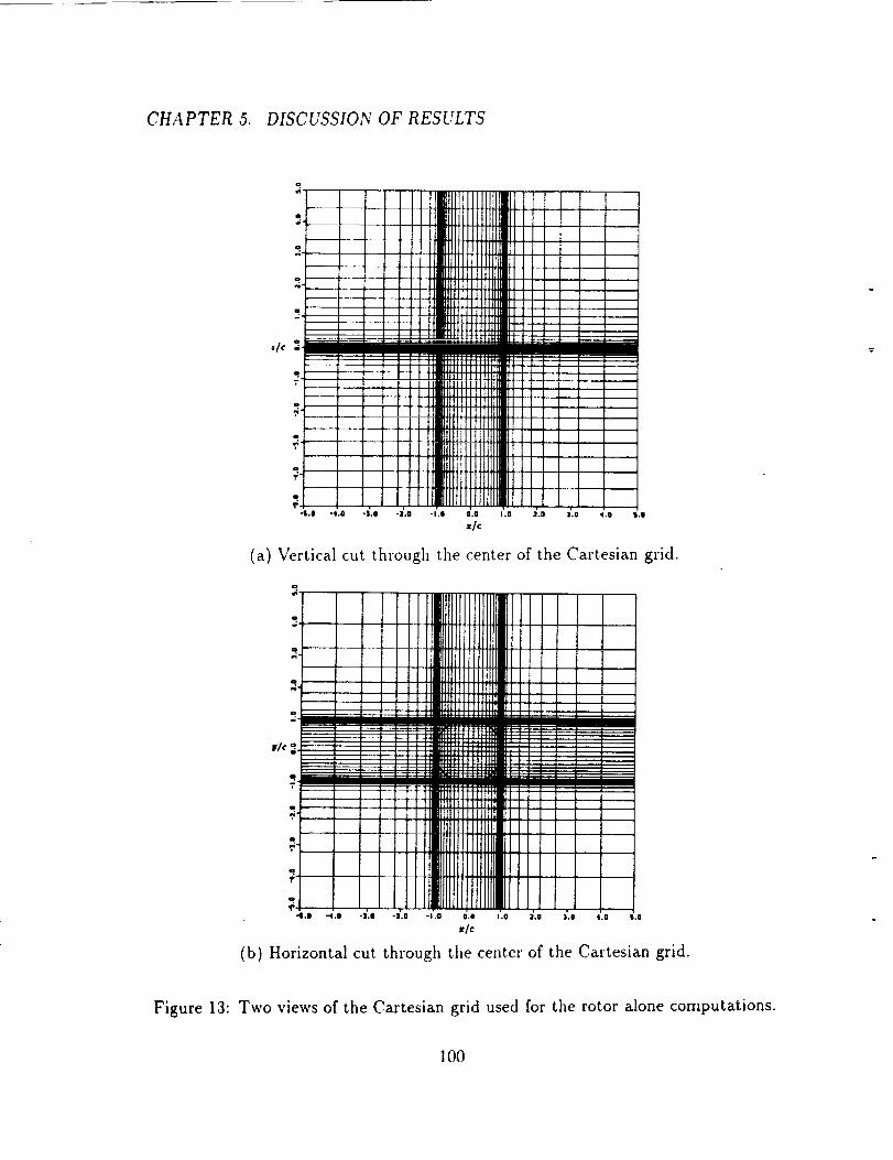
CHAPTER 5. DISCUSSION OF RESULTS
o
o.
?
./c _-
T"
o,N 4
o
o
2,-S.O -4.0 *_J.O -_i.O -I .e 0.0 l .O 2.0 3.0 4.0 5.11
s/¢
(a) Vertical cut through the center of the Cartesian grid.
w/c2.
o÷.
o,p"
o'r-
"S.O -4.0 -$.0 -]1.0 -J .0 O.O 1.0 2.0 3.0 4.0 S.O
s/c
(b) Horizontal cut through tile center of the Cartesian grid.
Figure 13: Two views of the Cartesian grid used for the rotor alone computations.
lOO

CHAPTER 5. DISCUSSION OF RESULTS
,
z/c _-
9-
" /T" , ,
- . o
Z/¢
Figure 14: Contours of pressure in a vertical plane through the rotor for a uniformly-loaded rotor with CT = 0.0164.
-I,0 0.0 1.0
z/c
Figure 15: Contours of velocity magnitude in a vertical plane through the rotor for a
uniformly-loaded rotor with CT = 0.0164.
101

CHAPTER 5. DISCUSSION OF RESULTS
o
it,o
o
16.o
o
,/c _.
1
t
t_
8
q
.... ,I _-_,
....... IlL
...... ,11 I
/ • / 4J_" --
7"11 ....11' .......
I1_' ......
11 I I I llliJ" ......
I1 I 1 I 1 I llil_" ......"7, , o , ,
II -n:w -ore ,14w -o• o:m o• o:m i:n i:m i,,
:/c
Figure 16: Velocity vectors in a vertical plane through the rotor for a uniformly-loaded
rotor with CT = 0.0164.
-']4_.0
40.0
_5.0- '+ "'%"°A
20.0,
_0
_0.0-
s.o!
10.0-
$,0-
0.0-
-$.0 -
-10.0
0.0
"liDb
_'" c/R * 100
.... "- ..... ., 0 (degs)
,lJ d._ ci.,, _.s d.o _i.:, d., d., _,o
RADIAL LOCATION (r/R)
Figure 17: The blade chord and twist distributions used for the non-uniformly-loaded
rotor model.
1O2

CHAPTER 5. DISCUSSION OF RESULTS
_.2-
2.0-
1.8-
1.G-
1.4-
1.2-
1.0-
0.8-
0.6-
0.4-
0.2-
0.0-
-0.2-
-0.4 -
-0.6.
-0.B-
-1.0-
-I.20.0
e!
e !
I_ ..................x_/_o/aeg_/r :_, -_..x..--..>,.,,c_• _o
: A. A'''" w:" ....... A ...... ,. ...... __...... Ao °
i
e
o., _-_ _._ o.4' c;s o.6' g., (/e _., to'RADIAL LOCATION (r/R)
Figure 18: Radial dist,'ibutions of blade loading and angle of attack for a non-
uniformly-loaded rotor with CT = 0.0164.
0.09 -
0.08-
0.07-
0.06-
0.05 -
0.04-
0.03-
0.02-
0.01-
0.000.0
v.
,,.A ....... A ....... l_.,
"A*" "°" ° A.., A
" _'A-. .... A°''°--A°*•'"
o, _.2 _3 o.4' ' 0'.6 d7 0.0.S 0.g '1.0
RADIAL LOCATION (r/R)
Figure 19: Radial distributions of axial velocity, 1,_ and swirl velocity' 1/, at the rotor
disk for a non-uniformly-loaded rotor with CT = 0.0164.
103

CHAPTER 5. DISCUSSION OF RESULTS
8
.°
_' I-QI D e.i
,.II?
! 3S -1.00 -O.rJ -O.SO "0 ;IS 0.00 0 _ O.SO 0.3_, I.OO I I* . . . .
zlc
Figure 20: Contours of pressure in a vertical plane through the rotor for a non-uni-
formly-loaded rotor with Cr = 0.0164.
o
..3-
_/¢
o
,r
II_|,i_ ll--
_
-4.0 -3.0 -3.0 -I .0 0.0 1.0 ;LO ].0 4.0 S.O
z/c
Figure 21: Contours of velocity magnitude in a vertical plane through the rotor for a
non-uniformly-loaded rotor with CT = 0.0164.
104

CHAPTER 5. DISCUSSION OF RESULTS
(a) Immediately above rotor.
' ' '"_ _ _ t t 1 t 1 I I I | I I t I I _ _,,,," •
..... '_ _ _ t i | I I I l I t _ _,,, .....
i iiiiiilII --_ lilIlii///;;..... .'.,._, i t t/./'_4,,,, .....
-"'" _ ! _ "/ Y/#/yZ_Z//,"m'" -
--h.__...,,, , ,,?..--.f_ _- "-V---"-" , " - "'' '";"_- -
I
- -_ ...... , , _ \'.\'-,.¢___ _
- -_.'."1__ /1 /J /.41 ,I I ! _b N....._- -
...... . . • • • a I I I I t 1 i _ • ,, .....
(b) Immediately below rotor.
Figure 22: Top view of the velocity vectors projected onto horizontal planes immedi-
ately above and below the ,'otor for a non-uniformly-loaded rotor computation.
105

CHAPTER 5. DISCUSSION OF RESULTS
(a) Side view.
(b) Top view.
Figure 23: Two views of the particle traces in the flowfield below a non-uniformly-
loaded rotor.
106

CHAPTER 5. DISCUSSION OF RESULTS
IJ.
i Ij,
i.o.
o._l-
,_l_ } CT ----0.00,51
..,O oo
o..D'" _I_°"°';..._,° .°°° "l
" °__ I'° ' Cr = 0.0164
]i _i a.D..O,."
o.a o.o _a d,, _.* o.o [o _._
RADIAL LOCATION (r/R)Gr e .ml| , r,XPI_I_AL
Or Imlt COMPtITIIDm. .
......... _r - Jl|4kl_ I_PI_I_AL
O Or - 0|k COMPIrf'¢D
Figure 24: Comparison of calculated and measured induced velocities about one wingchord below the rotor disk.
[,.,
_0
f,.
O
tL
1.O"
O.t-
0.0-
0.7-
0.6-
0.5-
0,4
0.3,
0.1-
°'°o.;_
C)
COMPUTATIONAL
EXPERIMENTAL
O.OtO O.0tS O._0
THRUST COEFFICIENT (Cr)
Figure 25: Comparison of calculated and measured values of figure of merit for a
range of thrust coefficients, for a rotor alone.
107

CHAPTER 5. DISCUSSION OF RESULTS
o'1
To
i
l I I I ||I 1 I| l
! Ii | I i i t , ' 1
. . .. \ \ \ _ I t t LlilIll I I I I I ! I I t e ' '
" i i ttltl]t/f!!
I 1_ l\_'' , '
• "'_'; . _ I I I lli|t, t , 1 L L ' ,,, , , , ,'
I I ,,1111| I I _ I ' ' ,I t t
0
Figure 26: Perspective view of the velocity vectors for wing/rotor interaction with
uniform rotor disk loading -- in a near-vertical plane running spanwise through the
wing mid-chord.
108

CHAPTER 5. DISCUSSION OF RESULTS
C_
111
,4-
0
e4-
0
el)
c;-
9-
0
I
i.
, w , w o o J _mtio i r p e _ • • • • • o o ° .
l I l t I t I i t i | I | l I | lllI| | 0 I I I • • * • • . B . e
0
0
-I.0 -0.5
f o u I 1 ! t t ! t I I i I ! ! IIlIII ! I ! I I I • • • _ w B o
I I I I I t t 1, t i t I I I I | IJl||
w I I t _ _ t _ I | I | ! I ! I I|tI|
, , , , I I I _ I l t t I I I I lllIl
i: .. trill
• ./_
LILIIJiIJ I II l llll i!!!1]1IiiLtt
rrrr,,ilIII .... I! o e # ii , w # _, # i t t • . .
! i i p F J I ! _ . . .
i _ p _ e o i t • . .._.
............ " "III#............ s M/_ri l............. ;, ,.-i_11
• , I i ii/lf '1'='"_111
/ I111 IIw _ i i _ i i a e e
t I I I , ! L I I I
I I I I I ! | I I I
I I I I I I I I | I
I , ! I ! ! I i # I
_;:: :
iiii0 • • •• , • ,
• . , o
e , • °
_ , ° .
d.o d.s ,% _.o
I I
n i / I I111_111I I I
# I IIIlll_li I I I 1 _ ,
I I IIIIWIIII I I I _ _ ,
I I I I IIIImll I I I 1 _
,',s _'.o _'.s _'.o {.s
Figure 27: Velocity vectors in a vertical plane running spanwise through the wing
mid-chord, for uniform rotor disk loading.
I09

CHAPTER 5. DISCUSSION OF RESULTS
?-
-I.O _.$ 0.0 O.S 1.0 I.S 3.0 _.S _.0 3.S 4.0 4.S $.0
Figure 28: Contours of velocity magnitude in a vertical plane running spanwise
through the wing mid-chord, for uniform rotor disk loading.
_q.
,/c :.
,_.
ml
-I.o 4.s i.o o'.s ,'.o ;.s _.o i.i i.o i.s _'.o ;.i i.ov/e
Figure 29: Contours of pressure in a vertical plane running spanwise through the
wing mid-chord, for uniform rotor disk loading.
110
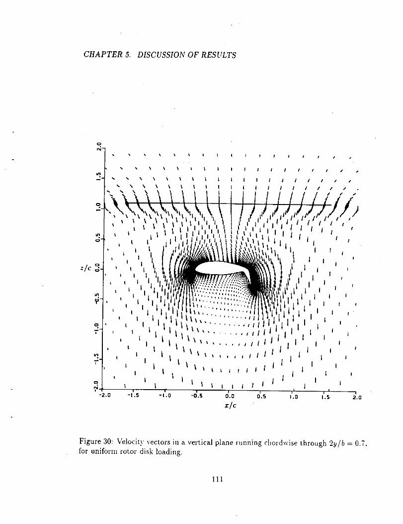
CHAPTER 5. DISCUSSION OF RESULTS
x/c
I I I I • •
I I I I / I •
I I I I I s •
I I I I / / /
Figure 30: Velocity vectors in a vertical plane running chordwise through 2y/b = 0.7,
for uniform rotor disk loading.
]ll

CHAPTER 5. DISCUSSION OF RESULTS
u
_'a.o -Ls -t.o -o.s g.o o'.s ,'.o i'.s e.oz/c
Figure 31: Contours of velocity magnitude-in a vertical plane running chordwise
through 2y/b = 0.7, for uniform rotor disk loading.
\",,',=..--J'//",,
_,o ,5 " (o 4s o*o _s :o :s io
z/c
Figure 32: Contours of pressure in a vertical plane running chordwise through 2y/b =
0.7, for uniform rotor disk loading.
112

CHAPTER 5. DISCUSSION OF RESULTS
2-D
1000.0 tSO0.O 2000.0
NON-DIMENSIONAL TIME (t i,./c)
Figure 33: Comparison of the time history of the ratio download/thrust between two-
and three-dimensional computations.
LEADING EDGE
WING TIP
WING ROOT
TRAILING EDGE
FLAPS 67"
Figure 34: The computed oil flow pattern on the wing upper surface, for uniform
rotor disk loading.
113

CHAPTER 5. DISCUSSION OF RESULTS
Is _g4_°
+=-:_
(a) Side view.
llll I_lill iJ(b) Front view.
(c) Top view.
Figure 35: Schematic of installation of the 0.658-scale V-22 wing and rotor in the
NASA Ames 40- by 80-Foot Wind Tunnel (taken from [10]).114

CHAPTER 5. DISCUSSION OF RESULTS
_-i.o -I.S -I'.O -O.S' _.e o'.s i'.o I'.s _.0
z_
(a) Immediately above rotor.
"1: !W!III ' ;
-l.o -I'.$ -I'.o -o.s o.o o.s I.o i.s l',o
x/c
(b) Immediately below rotor.
Figure 36: Top view of the velocity vectors projected onto horizontal planes immedi-
ately above and below the rotor for a wing and non-uniformly-loaded rotor computa-tion.
115

CHAPTER 5. DISCUSSION OF RESULTS
.j',
5°
q
_q
ROTOR
WING
Figure 37: The instantaneous particle traces in a near-vertical plane in the wing root
region showing the fountain flow, for non-uniform rotor disk loading.
116

CHAPTER 5. DISCUSSION OF RESULTS
LEADING EDGE
WING ROOT
WING TIP
TRAILING EDGE
FLA PS 67"
Figure 38: The computed oil flow pattern on the wing upper surface, for non-uniform
rotor disk loading.
2-
v/c =-
2-
?-].0 -_.S
= 0.332
-- --_- _/b,:0.145
-i.o -,'.,, -;.o 4., o'.o o'.s ,'.o ,'.s i.o ;.s _.oz/c
Figure 39: Sketch of the wing and rotor as seen from above, showing various spanwiselocations referred to in the discussion.
117

CHAPTER 5. DISCUSSION OF RESULTS
?
I
I 1I I
I / / / /
1 / / / ,,
t t / / /
Figure 40: Velocity vectors in a vertical plane running chordwise through 2y/b = 0.7,
for non-uniform rotor disk loading.
I18

CHAPTER 5. DISCUSSION OF RESULTS
• $ $ • _-'"_ .... NO SWIRL
=/c
Figure 41: Comparison of wing surface pressures at 2y/b = 0.7 showing the effect ofswirl.
119

CHAPTER 5. DISCUSSION OF RESULTS
tO
A
I 0.0.
-1.0.
-3.0
-3-1.0.0
21t/b J"0.145
x/c
a EXPEIUMEHTAL • COMPUTATIONAL
(a) 2y/b = 0.145
!.0.
• &- •. -- .. °.] &°'• "'A,.
_ -O J,
" 2mlb
-aLet -'" _°u | . , . , ., , , . , . ,
O.O 0.3 0.4 O.O 6.8 t@
z/¢
o F.,XPERJ,MENTAL • COMPUTATIONAL
(b) 2y/b = 0.332
Figure 42: Computed wing surface pressures compared with experimental results, for
non-uniform rotor disk loading.
120

CHAPTER 5. DISCUSSION OF RESULTS
IJ,
LO. A_'Jb° _lk" a- °A°" L*°&% &.. 6."
O..t-
'_ o,o:
-ql0,ll,
-3.0 1
-3.S
z/c
o F_PER]MENTAL • COMPUTATIONAL
_0
(c) 2y/b = 0.518
I.$.
to:
o,o
i -LO.
"1"11 il
2v/b = o._,-2.0
-3.1.
o.o _a * _.4 " d., " _.oz/¢
n EXPEPdMENTAL • COMPUTATIONAL
(d) 2y/b = 0.705
Figure 42: Continued.
I'.0
121

CHAPTER 5. DISCUSSION OF RESULTS
_.._ _.. :
-=.o 2rt/b - 0.891 "_
_so.o _ _., " _., " _..
=/c
o EXPEKIMENTAL 6 COMPUTATIONAL
I'.o
(e) 2y/b = 0.891
Figure 42: Concluded.
122

CHAPTER 5. DISCUSSION OF RESULTS
3.0.
I.O-
_a
NJ
O 0.S-3_
0.0,
0.0
• .// "x"_..A_PERIMENT
6+ d+ d,
SPANWISE LOCATION
EDGE
OF
ROTOR
1.0
Figure 43: Comparison between computed and measured values of the normalized,time-averaged download/thrust per unit span.
taO-
1.30.
I._IS -
l._O-
1.m-
t.lO-
l.OI.
1.00-
0.I$-
O.IO-
O.IS-
OiO
0.0
LOCATION
of
WINGA
i i i - ,
4_.o 0o o io • 3_o_]oo.o
AZIMUTHAL LOCATION _ (degs)
7310.0
V_/Vh
Ap/(T/A)
a/7 (degs)
Figure 44: The azimuthal variation of several parameters shows the influence of the
wing on the flow at the rotor disk at r/R = 0.60.
123

CHAPTER 5. DISCUSSION OF RESULTS
'i//,/./////, ,
/ / ll////_I/ I
(a) With no blowing.
1
1
1
"u//_/I iiiiiiii_/
- i\\\_" \• 11\ "'- _ r SEPAR,_'no_
, \ . ,\x' "xm..."
(b) With blowing, pp/poo = 1.04.
Figure 45: Close-up of velocity vectors near leading edge at 2y/b = 0.7 with and
without blowing
124

CHAPTER 5. DISCUSSION OF RESULTS
,//I//i
(_) With no blowing
t
jJ
(b) With blowing, pp/po_ = 1.04
Figure 46: Particle traces showing the wing wake at 2y/b = 0.7, with and without
blowing.
125

CHAPTER 5. DISCUSSION OF RESULTS
:__ _ WITHOUT BLOWING
I
_ "2"01 ":6_ _.._/',,,__> WITH BLOWING<
t._ -3.0.
'-4O
--$.0
0.0 _ _.4 J.6 d.e _.0
x/c
Figure 47: The computed wing surface pressures at 2y/b - 0.7 with and without
blowing.
0"132 1
0.131
O J30 l
/_ O.Q8,
_ °.Q,-I ._I /0J26
: 6
0.121-
*'_*,.oo"_o, ,.o,.........,.o, ,.o4 ,.os ,.o6 ,.o, ,.oe ,.0, _ {,, ,:5
Pp/P_
Figure 48: The variation of download/thrust with plenum blowing pressure.
126

CHAPTER 5. DISCUSSION OF RESULTS
0,00 0.05 0.10 0.1$ 0,20 0.3S 0.20
=/c
Figure 50: The wing surface pressures near the leading edge at a spanwise location
of 2y/b -- 0.7 for different blowing pressures.
127

CHAPTER 5. DISCUSSION OF RESULTS
Figure 51: Local download per unit span for a range of blowing pressures.
128

Chapter 6
Conclusions and
Recommendations
6.1 Conclusions
Computations of wing/rotor interaction about a tilt rotor configuration in hover have
been successfully performed. The three-dimensional, unsteady, thin-layer Navier-
Stokes equations are solved using a time-accurate, implicit, finite difference solution
algorithm. Previous attempts at computing the complex tilt rotor flowfield involved
solving either, in three-dimensions, a simpler set of equations that did not include vis-
cous effects, or, in two-dimensions, the Navier-Stokes equations for an airfoil at right
angles to the freestream. The flowfield about the tilt rotor configuration, however,
being very complex, and involving highly three-dimensional flow over the tilt rotor
wing with both leading and trailing edge flow separations, requires an approach such
as that developed in this work for an accurate computation of all the flow features.
The method developed here is unique in that it not only computes the time-
averaged rotor flowfield including the mean axial and swirl velocity components in
the rotor slipstream, but does so in the presence of a bluff body, i.e. the wing. The
rotor flow and the flow about the wing are closely-coupled, the rotor disk being only
about one wing chord above the wing. Both the effect of the rotor flowfield on the
wing and the effect of the wing on the rotor flow are computed with the current
129

CHAPTER 6. CONCLUSIONS AND RECOMMENDATIONS
numerical model. This is accomplished by modeling the rotor as an actuator disk
and incorporating momentum theory/blade element analysis into the Navier-Stokes
solution method. Solution blanking at interior points of the mesh has been shown
here to be an effective technique in introducing the effects of the rotor and tangential
leading edge jet. In this way, only a single-zone grid is required to represent the wing,
rotor disk, and tangential wall jet.
The computational method developed in this work is useful in gaining a more
detailed understanding of the complex tilt rotor flowfield in hover. The principal
observations from the numerical results are outlined below:
The three-dimensionality of the flow around the wing is highlighted by the
transitioning of primarily chordwise flow on the wing upper surface to primarily
spanwise flow further inboard.
The vertical extent of the fountain flow at the plane of symmetry is less than
observed in flow visualization during experimental tests, indicating that, within
the limitations of the present analysis, the effect of the fountain is less important
than previously thought.
The spanwise variation in the flowfield is also clearly evidenced in the computed
variation of download along the wing. The download is greater on that portion
of the wing immersed in the rotor flowfield, as expected, but also it is increased
locally in the region of the recircuIation fountain.
The flow separates from the wing leading and trailing edges, creating a large
region of separated flow beneath the wing. The computation indicates that
the resulting flow unsteadiness' is very small. This observation is supported
by experimental results which indicate that the measured unsteadiness is due
primarily to the unsteady rotor wake caused by rotor blade passage, which is
not modeled in the current numerical approach.
• Flow separation forward of the trailing edge on the flap upper surface is pre-
dicted for that region of the wing where the flow is generally chordwise. This
130

CHAPTER 6. CONCL USIONS AND RECOMMENDATIONS
emphasizes the need to optimize flap angle and flap surface profile in order to
minimize early flow separation which increases the wing download.
• The computation predicts the formation of a standing vortex beneath the wing
tip. This has not as yet been observed experimentally.
The azimuthal variation of flow properties in the rotor disk, due to the blockage
effect of the wing, is of sufficient magnitude that it should be accounted for in
stability and control and vibration analyses of the tilt rotor.
The benefits of a numerical model are highlighted in the study of the effects
of rotor-induced swirl. By being able to turn it off and on, computationally,
which can not be done experimentally, swirl is seen to be beneficial, by reducing
download.
Leading edge tangential blowing is effective in reducing the download. As-
suming that the payload is 25% of the total rotor thrust, the 7% computed
reduction in download due to blowing would yield a not insignificant increase
in payload carrying capability of about 3 - 4%, depending on the actual magni-
tude of download/thrust. Optimum blowing would involve a spanwise variation
of plenum pressure, with more blowing required on that portion of the wing
immersed in the rotor flowfield, and also in the fountain region. Greater reduc-
tions in download could probably be obtained by tailoring the shape of the wing
leading edge to be a better Coanda surface. An optimization of the location of
the jet would also be a useful exercise.
Comparisons have been made between computational results and experimental
measurements, but with some caution. The numerical model of the tilt rotor differs
somewhat from the experimental models. For example, the nacelle, rotor hub, and
model support structures are not represented in the computa-tion. Wing sweep and
dihedral, which probably tend to reduce the download, are also not taken into account.
The predicted wing download is 20%-30% higher than the measured values at a rotor
thrust coiffficient of 0.0164. In summary, the discrepancies with experiment are mainly
due to the following:
131

CHAPTER 6. CONCLUSIONS AND RECOMMENDATIONS
• Differences between the numerical and experimental model configurations.
• Insufficient grid point density and less-than-optimum grid point distributions
that contribute to numerical dissipation and local inaccuracies in resolution of
the flow.
• Limitations inherent in the thin-layer Navier-Stokes equations.
• Limitations of the turbulence models.
Despite the limitations listed above, the numerical model developed in this work
has proven to be a useful tool in studying the tilt rotor flowfieId and download re-
duction due to leading edge tangential blowing. It can also be used to examine such
things as the effect of flap deflection, direction of rotor rotation, and rotor thrust
coefficient on download.
6.2 Recommendations
When the experimental results become available, from on-going tests at NASA Ames
of a tilt rotor configuration which is near-identical to the computational model, com-
parison with the current numerical results would be very useful. This would provide
a more accurate basis of comparison by eliminating discrepancies due to geometric
differences.
Further improvements in the accuracy of the computation could be obtained by
increasing the grid point density in the regions of the rotor and rotor wake, particu-
larly, near the edge of the rotor slipstream. The grid density could also be increased
around and beneath the wing to better resolve the complex flow in the wing wake.
Further grid sensitivity studies are required to determine more completely the effect
of the grid on the solution.
Because the local download distribution along the wing is sensitive to the local
induced velocity distribution beneath the rotor, to improve the accuracy of the total
download prediction, the rotor induced velocity must be more accurately computed.
The current grid is Cartesian-like in and below the rotor plane and, therefore, it is
132

CHAPTER 6. CONCLUSIONS AND RECOMMENDATIONS
not capable of accurately resolving the edge of the rotor slipstream for all azimuthal
locations. It is suggested that this be achieved by exploiting the current method's
"blanking" capability and expanding it to a full "chimera" implementation. This
would permit the embedding of a cylindrical grid into a global grid around the wing.
The cylindrical grid would provide a more appropriate distribution of points for the
resolution of the cylindrically-shaped rotor slipstream. The solutions of each mesh
would be performed consecutively and boundary conditions updated by interpolation
between grids.
The rotor's effect on the flowfield is unsteady and caused by the passage of each
blade. In the case of the 3-bladed V-22 rotor, for example, any given point on the
rotor disk sees a 3-per-rev forcing frequency. In the current study, the unsteady effects
of the rotor blades are time-averaged onto elemental areas of the rotor disk. Given
sufficient number of grid points in the rotor plane, however, the effective position of
the blades could be resolved and the local, time-dependent contribution of the blades
could be modeled. In this way the effects on wing download, of unsteadiness imparted
by the rotor into the slipstream, could be studied.
An experimental test of a model wing at right angles to a freestream flow would
help gain a better understanding of the complicated flow region beneath the wing, in
the absence of the cyclic pulsing imparted to the flowfield by the rotor. This would
allow measurement of the unsteadiness in the wing wake and its consequent effect on
the magnitude and frequency of download oscillations. In order to either validate the
current computation or provide guidance for further improvements to the numerical
model, it would be useful to know whether the actual wing wake is comprised of a
vortex street or a pair of counter-rotating vortices (as computed), or whether it is
more random and chaotic (and, therefore, much more difficult to model numerically).
A greater degree of accuracy in the modeling of the separated flow region would
be attained if the full Navier-Stokes equations are solved. Also, an improved tur-
bulence model developed specifically for bluff body flows would improve the results
even further. A computation which is second-order accurate in time might also be
attempted to better resolve the unsteadiness in the wake.
Eventually, at some point in the future when computational resources become
133

CHAPTER 6. CONCLUSIONS AND RECOMMENDATIONS
available, it would be desirable to perform a time-accurate Navier-Stokes calculation
about each of the rotating blades of the rotor and to couple that with the solution
of the rest of the tilt rotor flowfield. Modeling the rotor hub, engine pylon, the
fuselage and tail are obvious improvements that would help yield a more accurate
representation of the actual tilt rotor aircraft. This, of course, would entail complex
grid generation.
Implementation of all the above recommendations is a challenging task, but one
that would be of great value in the pursuit of the complete understanding of the
complicated tilt rotor flowfield.
134

Bibliography
[1] Rosenstein, H. and Clark, R., "Aerodynamic Development of the V-22 Tilt Ro-
tor", AIAA Paper 86-2678, AIAA/AHS/ASEE Aircraft Systems, Design _z Tech-
nology Meeting, Dayton, Ohio, 1986.
[2] Felker, F. F. and Light, J., "Rotor/Wing Aerodynamic Interactions in Hover",
NASA TM 88255, 1986.
[3] McVeigh, M. A., "The V-22 Tilt-Rotor Large-Scale Rotor Performance/Wing
Download Test and Comparison with Theory", Vertica, Vol. 10, No. 3/4, 1986.
[4] Maisel, M. and Harris, D., "Hover Tests of the XV-15 Tilt Rotor Research Air-
craft", AIAA Paper 81-2501, AIAA/SETP/SFTE/SAE/ITEA/IEEE 1st Flight
Test Conf., Las Vegas, 1981.
[5] McCroskey, W., Spalart, P., Laub, G., Maisel, M., and Maskew, B., "Airloads on
Bluff Bodies, with Application to the Rotor-Induced Downloads on Tilt-Rotor
Aircraft", Vertica, Vol.9, No.l, 1985.
[6] Felker, F. F., "A Review of Tilt/Rotor Download Research", Paper No. 14, 14th
European Rotorcraft Forum, Milano, Italy, 1988.
[7] Maisel, M., Laub, G., and McCroskey, W., "Aerodynamic Characteristics of
Two-Dimensional Wing Configurations at Angles of Attack Near -90 °', NASA
TM 88373, 1986.
135

BIBLIOGRAPHY
[8]
[9]
[lO]
[11]
[121
[13]
[14]
[15]
[16]
McVeigh, M., Grauer, W., and Paisley, D., "Rotor/Airframe Interactions on
Tiltrotor Aircraft", Proceedings of the 44th Annual Forum of the American
Helicopter Society, Washington, D.C., June 1988.
Felker, F., Signor, D., Young, L., and Betzina, M., "Performance and Loads Data
From a Hover Test of a 0.658-Scale V-22 Rotor and Wing", NASA TM 89419,
April 1987.
Felker, F., Shinoda, P., Heffernan, R., and Sheehy, H., "Wing Force and Surface
Pressure Data from a Hover Test of a 0.658-Scale V-22 Rotor and Wing", NASA
TM 102244, Feb. 1990.
Felker, F., "Results from a Test of a 2/3-Scale V-22 Rotor and Wing in the 40-
by 80-Foot Wind Tunnel", presented at the 47th Annual Forum of the American
Helicopter Society, Phoenix, Arizona, May 1991.
Clark, D. and McVeigh, M., "Analysis of the Wake Dynamics of a Typical Tilt-
Rotor Configuration in Transition Flight", Paper No. 28, l lth European Rotor-
craft Forum, London, England, 1985.
Clark, D., "Analysis of the Wing/Rotor and Rotor/Rotor Interactions Present
in Tilt-Rotor Aircraft", Vertica, Vol.ll, No.4, 19871
Lee, C. S., "Panel Method Calculation of Tilt Rotor Download", Paper 39-1,
presented at the International Specialists' Meeting on Rotorcraft Basic Research,
Atlanta, Georgia, March 1991.
Lee, C. S., "A Two Dimensional Study of Rotor/Airfoil Interaction in Hover",
JIAA TR-88, Stanford University, 1988.
Raghavan, V., McCroskey, W. J., Van Dalsam, W. R., and Baeder, J. D., "Cal-
culations of the F10w Past Bluff B0dies, Including Tilt'Rot0r Wing Sections at
a = -90 °", AIAA Paper 90-0032, A!AA 28th Aerospace Sciences Meeting, Reno,
1990.
136
BIBLIOGRAPHY
[17]
[18]
[19]
[20]
[21]
[22]
[23]
[24]
[25]
[26]
Stremel, P. M., "Calculation of Flow about Two-Dimensional Bodies by Means of
the Velocity-Vorticity Formulation on a Staggered Grid", AIAA Paper 91-0600,
AIAA 29th Aerospace Sciences Meeting, Reno, 1991.
Johnson, W., Helicopter Theory, Princeton University Press, Princeton, New
Jersey, 1980.
Stremel, P. M., "A Method for Modeling Finite Core Vortices in Wake Flow
Calculations", AIAA Paper 84-0417, AIAA 22nd Aerospace Sciences Meeting,
Reno, 1984.
Stremel, P. M., "The Calculation of Rotor/Fuselage Interaction for Two-
Dimensional Bodies", 16th European Rotorcraft Forum, Paper II.11.3, Glasgow,
Sept. 18-21, 1990.
Srinivasan, G. and McCroskey, W., "Numerical Simulations of Unsteady Airfoil-
Vortex Interactions", Vertica, Vol. 11, No.1/2, 1987.
Agarwal, R. K. and Deese, J. E., "Euler Calculations for Flowfield of a Helicopter
Rotor in Hover", J. Aircraft, Vol. 24, No. 4, April 1987.
Roberts, T. W., "Euler Equation Computations for the Flow Over a Hovering
Helicopter Rotor", NASA CR 177493, 1988.
Srinivasan, G. and McCroskey, W., "Navier-Stokes Calculations of Hovering Ro-
tor Flowfields", AIAA Paper 87-2629-CP, AIAA Atmospheric Flight Mechanics
Conf., Monterey, California, 1987.
Srinivasan, G. R., Baeder, J. D., Obayashi, S., McCroskey, W. J., "Flowfield of
a Lifting Hovering Rotor -- A Navier-Stokes Simulation", Paper No. 1.3.5, 16th
European Rotorcraft Forum, Glasgow, Scotland, Sept. 1990.
Rajagopalan, R. G. and Mathur, S. R., "Three Dimensional Analysis of a Rotor
in Forward Flight", AIAA Paper 89-1815, AIAA 20th Fluid Dynamics, Plasma
Dynamics and Lasers Conf., Buffalo, 1989.
137

BIBLIOGRAPHY
[27] McCroskey, W. and Baeder, J., "Some Recent Advances in Computational Aero-
dynamics for Helicopter Applications", NASA TM 86777, 1985.
[28] Obayashi, S. and Kuwahara, K., "An Approximate LU Factorization Method for
the Compressible Navier-Stokes Equations", Journal of Computational Physics,
Vol.63, 1986.
[29] Fujii, K. and Obayashi, S., "Practical Applications of New LU-ADI Scheme for
the Three-Dimensional Navier-Stokes Computation of Transonic Viscous Flows",
AIAA Paper 86-0513, AIAA 24th Aerospace Sciences Meeting, Reno, 1986.
[30] Fujii, K. and Obayashi, S., "Navier-Stokes Simulation of Transonic Flow over
Wing-Fuselage Combinations", AIAA Paper 86-1831, AIAA 4th Applied Aero-
dynamics Conf., San Diego, 1986.
[31] Yeh, D., Tavella, D., Roberts, L., and Fujii, K., "Navier-Stokes Computation of
the Flow Field over Delta Wings with Spanwise Leading Edge Blowing", AIAA
Paper 88-2558-CP, AIAA 6th Applied Aerodynamics Conference, Williamsburg,
Virginia, June 1988.
[32] Yeh, D., Tavella, D., Roberts, L., and Fujii, K., "Numerical Study of the Effects
of Tangential Leading Edge Blowing on Delta Wing Vortical Flow", AIAA Paper
89-0341, AIAA 25th Aerospace Sciences Meeting, Reno, 1989.
[33] Yeh, D., "Numerical Study of Delta Wing Leading Edge Blowing", JIAA TR-86,
Stanford University, 1988.
[34] Benek, J. A., Buning, P. G., and Steger, J. L., "A 3-D Chimera Grid Embedding
Technique", AIAA Paper 85-1523, 1985.
[35] Liepmann, H. W. and Roshko, A., Elements of Gasdynamics, John Wiley &
Sons, Inc., New York, 1957.
[36] Viviand, H., "Formes Conservatives des l_quations de la Dynamique des Gaz',
LaRecherche A_rospatiale, No.I, 1974.
138

BIBLIOGRAPHY
D
[37]
[38]
[39]
[40]
[41]
[42]
[43]
[44]
[45]
[46]
Vinokur, M., "Conservation Equations of Gasdynamics in Curvilinear Coordi-
nate Systems", Journal of Computational Physics, No.14, 1974.
Anderson, D. A., Tannehill, J. C., and Pletcher, R. H.,
Computational Fluid Mechanics and Heat Transfer, Hemisphere
Corp., New York, 1984.
Publishing
Baldwin, B. and Lomax, H., "Thin Layer Approximation and Algebraic Model
for Separated Turbulent Flows", AIAA Paper 78-257, AIAA 16th Aerospace
Sciences Meeting, Huntsville, Alabama, 1978.
Roberts, L., "A Theory for Turbulent Curved Wall Jets", AIAA Paper 87-0004,
AIAA 25th Aerospace Sciences Meeting, Reno, 1987.
Shrewsbury, G., "Numerical Evaluation of Circulation Control Airfoil Per-
formance Using Navier-Stokes Methods", AIAA Paper 86:0286, AIAA 24th
Aerospace Sciences Meeting, Reno, 1986.
Beam, R. M. and Warming, R. F., "An Implicit Finite-Difference Algorithm
for Hyperbolic Systems in Conservation-Law Form", Journal of Computat!onal
Physics, Vol.22, 1976.
Pulliam, T. and Steger, J., "Implicit Finite-Difference Simulations of Three-
Dimensional Compressible Flow", AIAA Journal, Vol.18, No.2, 1980.
Meakin, R. and Suhs, N., "Unsteady Aerodynamic Simulation of Multiple Bodies
in Relative Motion", AIAA Paper 89-1996-CP, AIAA 9th CFD Conf., Buffalo,
June 1989.
Kuan, J.-H. and Dougherty, F. C., "Time Accurate Study for Multiple Moving
Grids", AIAA Paper 89-1997-CP, AIAA 9th CFD Conf., Buffalo, June 1989.
Pulliam, T. and Chaussee, D., "A Diagonal Form of an Implicit Approximate-
Factorization Algorithm", Journal of Computational Physics, Vol.39, 1981.
139

BIBLIOGRAPHY
[47]
[48]
[49]
[50]
[51]
[52]
[53]
[54]
Pulliam, T., "Euler and Thin Layer Navler-Stokes Codes: ARC2D, ARC3D",
Notes for Computational Fluid Dynamics User's Workshop, The University of
Tennessee Space Institute, Tullahoma, Tennessee, March 12-16, 1984.
Guruswamy, G. P., "Time-Accurate Unsteady Aerodynamic and Aeroelas-
tic Calculations of wings Using Euler Equations", AIAA Paper 88-2281,
AIAA/ASME/ASCE/AHS 29th Structures, Structural Dynamics and Materi-
als Conf., williamsburg: virginia, 1988:
Guruswamy, G. P., "Numerical Simulation of Vortical Flows on Flexible Wings",
AIAA Paper 89-0537, AIAA 27th Aerospace Sciences Meeting, Reno, 1989.
Steger, J. and Warming, R., "Flux Vector Splitting of the Inviscid Gasdynamic
Equations with Application to Finite-Difference Methods", Journal of Compu-
tational Physics, Vol.40, 1981.
Lombard, C., Bardina, J., Venkatapathy, E., and Oliger, J., "Multi-Dimensional
Formulation of CSCM - An Upwind Flux Difference Eigenvector Split Method
for the Compressible Navier-Stokes Equations", AIAA Paper 83-1895, AIAA 6th
CFD Conf., Danvers, Massachusetts, 1983.
Pulliam, T. and Steger, J., "Recent Improvements in Efficiency, Accuracy, and
Convergence for Implicit Approximate Factorization Algorithms", AIAA Paper
85-0360, AIAA 23rd Aerospace Sciences Meeting, Reno, 1985.
Obayashi, S. and Guruswamy, G. P., "Unsteady Shock-Vortex Interaction on a
Flexible Delta Wing", Paper AIAA 91-1109, 32nd AIAA/ASME/ASCE/AHS/-
ASC Structures, Structural Dynamics and Materials Conf., Baltimore, April
1991.
Obayashi, S., Fujii, K., and Gavali, S., "Navier-Stokes Simulation of Wind-
Tunnel Flow Using LU-ADI Factorization Algorithm", NASA TM 100042, Feb.
1988.
Q
140

BIBLIOGRAPHY
[55] Obayashi, S., "Numerical Simulation of Underexpanded Plumes Using Upwind
Algorithms", AIAA Paper 88-4360-CP, AIAA Atmospheric Flight Mechanics
Conf., Minneapolis, 1988.
[56] Steger, J., "Implicit Finite Difference Simulation of Flow About Arbitrary Ge-
ometries with Application to Airfoils", AIAA Paper 77-665, AIAA 10th Fluid &
Plasmadynamics Conf., Albuquerque, New Mexico, 1977.
[57] Sorenson, R. and Steger, J., "Numerical Generation of Two-Dimenslonal Grids
by the Use of Poisson Equations with Grid Control at the Boundaries", Proc. of
the Numerical Grid Generation Techniques Workshop, Langley Research Center,
NASA, Hampton, Va., NASA CP-2166, 1980.
[58] Thompson, J., Thames, F., and Mastin, C., "Automatic Numerical Generation of
Body-Fitted Curvilinear Coordinate System for Field Containing Any Number of
Arbitrary Two-Dimensional Bodies", Journal of Computational Physics, Vol. 15,
1974.
[59]
[6o]
[61]
[62]
[63]
Thompson, J., Thames, F., Mastin, C., and Shanks, S., "Use of Numerically
Generated Body-Fitted Coordinate Systems for Solutions of the Navier-Stokes
Equations", AIAA 2nd CFD Conf., Connecticut, 1975.
Holst, T. L., "Numerical Computation of Transonic Flow Governed by the Full-
Potential Equation", NASA TM 84310, 1983.
Sorenson, R., "A Computer Program to Generate Two-Dimensional Grids About
Airfoils and Other Shapes by the Use of Poisson's Equation", NASA TM 81198,
May 1980.
Chaussee, D., Kutler, P., and Pulliam, T. , "Three Dimensional Viscous
Flow Field Program. Part 1. Viscous Blunt Body Program (Interim Report)",
AFWAL-TM-81-63-FIMG, Flight Dynamics Laboratory, Air Force Wright Aero-
nautical Laboratories, Wright-Patterson Air Force Base, Ohio, 1981.
Glauert, H., The Elements of Airfoil and Airscrew Theory, Cambridge Univer-
sity Press, London, 1930.
141

BIBLIOGRAPItY
[64]
[65]
[66]
[67]
[68]
[69]
[70]
[71]
[72]
[73]
McCormick, B. W., Aerodynamics of V/STOL Flight, Academic Press, New
York, 1967.
Prouty, R. W., Helicopter Performance, Stability, and Control, PWS Publishers,
Boston, 1986.
Yu, N. J., Samant, S. S., and Rubbert, P. E., "Flow Prediction for Propfan
Configurations Using Euler Equations", AIAA Paper 84-1645, AIAA 17th Fluid
Dynamics, Plasma Dynamics and Lasers Conf., Colorado, 1984.
Oates, G. C., Aerothermodynamics of Gas Turbine and Rocket Propulsion,
American Institute of Aeronautics and Astronautics, Inc., New York, 1984.
Stepniewski, W. Z., "Rotary-Wing Aerodynamics. Volume 1 -- Basic Theories
of Rotor Aerodynamics (With Application to Helicopters)", NASA CR-3082,
January 1979.
Press, W., Flannery, B., Teukolsky, S., and Vetterling, W.,
Numerical Recipes The Art of Scientific Computing, Cambridge
Press, New York, 1987.
University
Tavella, D., Schiff, L., and Cummings, R., "Pneumatic Vortical Flow Control at
High Angles of Attack", AIAA Paper 90-0098, 28th Aerospace Sciences Meeting,
Reno, 1990.
Buning, P. and Steger, J., "Graphics and Flow Visualization in Computational
Fluid Dynamics", AIAA Paper 85- 1507, AIAA 7th CFD Conf., Cincinnati, 1985.
Walatka, P. and Buning, P., "PLOT3D User's Manual", NASA TM 101067,
1989.
Fejtek, I. and Robertsi L., "A CFD Study of Tilt Rotor Flowfields", JIAA TR-96,
Stanford University, 1989.
142

Form ApprovedREPORT DOCUMENTATION PAGE oM8No.o7o4-ola8
Public reporting burden for this collection of information is estimated to average 1 hour per response, including the time for reviewing insiructJons_ Searching existing data sources.gathering and maintaining the data needed, and completing and reviewing the collection of information. Send comments regarding this burden estimate or any other aspect of thiscollection of information, including suggestions for reducing this burden, to Washington Headquarters Services. Directorate for information Operations and Reports, 1215 JeffersonDavis Highway. Suite 1204, Arlington, VA 22202-4302, and to the Office of Management and Budget, Paperwork Reduction Pro ect (0704-0188). Washington, DC 20503.
1. AGENCY USE ONLY (Leave blank) 2. REPORT DATE 3. REPORT TYPE AND DATES COVERED
July 1993 Contrac!or,,Report4. TITLE AND SUBTITLE 5. FUNDING NUMBERS
Navier-Stokes Flowfield Computation of Wing/Rotor Interaction for aTilt Rotor Aircraft in Hover
6. AUTHOR(S) NCC2-55
Ian G. Fejtek
7. PERFORMING ORGANIZATION NAME(S) AND ADDRESS(ES) 8. PERFORMING ORGANIZATIONREPORT NUMBER
Stanford University
Department of Aeronautics.and Astronautics A-93096
Stanford, CA 94305
II I II
9. SPONSORING/MONITORING AGENCY NAME(S) AND ADDRESS(ES) 10. SPONSORING/MONITORING
AGENCY REPORT NUMBER
National Aeronautics and Space AdministrationNASA CR-4532Washington, DC 20546-0001
11. SUPPLEMENTARY NOTES
Point of Contact: Jeffrey Light, Ames Research Center, MSTO42, Moffett Field, CA 94035-I000; (415) 604-4881
12a. DISTRIBUTION/AVAILABILITY STATEMENT
Unclassified - Unlimited
Subject Category 02
12b. DISTRIBUTION CODE
blowing would involve a spanwise variation in blowing strength.
14. SUBJECT TERMS
Tilt rotor download, Computational fluid dynamics, Rotor/Wi2m interaction
17. SECURITY CLASSIFICATIONOF REPORT
Unclassified
NSN 7,540-01-280-5500
18. SECURITY CLASSIFICATIONOF THIS PAGE
Unclassified
15. NUMBER OF PAGES
156I[
16. PRICE CODE
A0819. SECURITY CLASSIFICATION 20. LIMITATION OF ABSTRACT
OF ABSTRACT
Standard Form 298 (Rev. 2-89)PTescrlbed by ANSI Std, Z3g-18
298 - 102
13. ABSTRACT (Maximum 200 words)
The download on the wing produced by the rotor-induced downwash of a tilt rotor aircraft in hover is of major concern because of its
severe impact on payload-carrying capability. A method has been developed to help gain a better understanding of the fundamental fluid
dynamics that causes this download, and to help find ways to reduce it. In particular, the method is employed in this work to analyze the effect
of a tangential leading edge circulation-control jet on download reduction. Because of the complexities associated with modeling the complete
configuration, this work focuses specifically on the wing/rotor interaction of a tilt rotor aircraft in hover. The three-dimensional, unsteady,
thin-layer compressible Navier-Stokes equations are solved using a time-accurate, implicit, finite difference scheme that employs LU-ADI
factorization. The rotor is modeled as an actuator disk which imparts both a radical and an azimuthal distribution of pressure rise and swirl
to the flowfield. A momentum theory/blade element analysis of the rotor is incorporated into the Navier-Stokes solution method. Solution
blanking at interior points of the mesh has been shown here to be an effective technique in introducing the effects of the rotor and tangential
leading edge jet. Results are presented both for a rotor alone and for wing/rotor interaction. The overall mean characteristics of the rotor
flowfield are computed including the flow acceleration through the rotor disk, the axial and swirl velocities in the rotor downwash, and the
slipstream contraction. Many of the complex tilt rotor flow features are captured including the highly three-dimensional flow over the wing,
the recirculation fountain at the plane of symmetry, wing leading and trailing edge separation, and the large region of separated flow beneath
the wing. Mean wing surface pressures compare fairly well with available experimental data, but the time-averaged download/thrust ratio
is 20-30% higher than the measured value. The discrepancy is due to a combination of factors that are discussed. Leading edge tangential
blowing, of constant strength along the wing span, is shown to be effective in reducing download. The jet serves primarily to reduce thepressure on the wing upper surface. The computation clearly shows that, because of the three-dimensionality of the flowfield, optimum
i


National Aeronautics and
Space Administration
Ames Research Center
Moffett Field, California 94035-1000
Official Business
Penalty for Private Use $300
BULK RATE
POSTAGE & FEES PAID
NASA
PermitNo. G-27


![Compact ink recirculation system CC1 - Toshiba Tec Top Page...Compact ink recirculation system Example: Mounting of ink recirculation system [CC1] with ink recirculation head Up to](https://static.fdocuments.net/doc/165x107/5f0f72527e708231d4443441/compact-ink-recirculation-system-cc1-toshiba-tec-top-page-compact-ink-recirculation.jpg)