Ignition Rate Measurement of Laser-Ignited Coals; 10/97; …/67531/metadc670601/m2/1/high... ·...
86
IGNITION RATE MEASUREMENT OF LASER-IGNITED COALS FINAL TECHNICAL REPORT 08/01/97 TO 07/31/97 AUTHORS: JOHN C. CHEN VINAYAK KABADI REPORT ISSUE DATE: 10/31/97 DE-FG22-94MT94012 --12 NORTH CAROLINA A&T STATE UNIVERSITY DEPARTMENT OF MECHANICAL ENGINEERING 1601 E. MARKET STREET GREENSBORO, NC 27411
Transcript of Ignition Rate Measurement of Laser-Ignited Coals; 10/97; …/67531/metadc670601/m2/1/high... ·...

IGNITION RATE MEASUREMENT OF LASER-IGNITED COALS
FINAL TECHNICAL REPORT
08/01/97 TO 07/31/97
AUTHORS: JOHN C. CHENVINAYAK KABADI
REPORT ISSUE DATE: 10/31/97
DE-FG22-94MT94012 --12
NORTH CAROLINA A&T STATE UNIVERSITYDEPARTMENT OF MECHANICAL ENGINEERING
1601 E. MARKET STREETGREENSBORO, NC 27411

Disclaimer
This report was prepared as an account of work sponsored by anagency of the United States Government. Neither the United StatesGovernment nor any agency thereof, nor any of their employees,makes any warranty, express or implied, or assumes any legal liabilityor responsibility for the accuracy, completeness, or usefulness of anyinformation, apparatus, product, or process disclosed, or representsthat its use would not infringe privately owned rights. Referenceherein to any specific commercial product, process, or service by tradename, trademark, manufacturer, or otherwise does not necessarilyconstitute or imply its endorsement, recommendation, or favoring bythe United States Government or any agency thereof. The views andopinions of authors expressed herein do not necessarily state or reflectthose of the United States Government or any agency thereof.
2
Abstract
We have established a novel experiment to study the ignition of pulverized coals under
conditions relevant to utility boilers. Specifically, our aims were to determine the ignition
mechanism, which is either homogeneous or heterogeneous, of pulverized coal particles under
various conditions of particle size, coal type, and freestream oxygen concentration. Furthermore,
we will measure the ignition rate constants of various coals by direct measurement of the particle
temperature at ignition, and incorporating this measurement into a mathematical model for the
ignition process. All of the above objectives were met by the project.
The ignition mechanism of pulverized coals in this experiment, under all conditions
examined, was determined by high-speed photography to be heterogeneous. That is, ignition of the
particles always occurred on the solid surface, prior to the evolution of volatile matter from the
particles into the gas phase. This finding was most likely due to the high heating rates achieved
(>105) by the laser heating, which causes the particle temperature to rise above that necessary for
ignition before appreciable devolatilization occurred.
Particle temperature at ignition was measured for one size group of one coal (Pittsburgh #8,
high-volatile bituminous) under two oxygen concentrations. These temperatures were analyzed
using a model of heterogeneous coal ignition developed by our group, and ignition rate constants
were determined.
3
Table of Contents
Disclaimer ...........................................................................................................................................................1
Abstract ...............................................................................................................................................................2
Table of Contents..............................................................................................................................................3
Executive Summary...........................................................................................................................................5
Introduction .......................................................................................................................................................8
Objectives .........................................................................................................................................................10
Results and Discussion ...................................................................................................................................11
I. Experiment Development....................................................................................................................11
A. Experiment Overview...................................................................................................................11
B. Coal preparation and handling ....................................................................................................12
C. Gas-handling system .....................................................................................................................14
D. Wind tunnel....................................................................................................................................16
E. Laser system and associated optics.............................................................................................18
F. Experiment procedure..................................................................................................................18
G. Two-color pyrometry system ......................................................................................................21
1. Theory of Operation.....................................................................................................................21
2. System Design................................................................................................................................28
3. Calibration Procedure ...................................................................................................................33
II. Data Reduction Methodology .............................................................................................................33
III. Ignition-Frequency Distribution Data..............................................................................................39
Pittsburgh # 8 – high-volatile A bituminous .....................................................................................40
Sewell – medium volatile bituminous ..................................................................................................43
Wyodak – subbituminous......................................................................................................................44

4
Illinois #6 – high-volatile C bituminous .............................................................................................46
IV. Temperature Measurements...............................................................................................................46
V. Ignition-Rate Data .................................................................................................................................52
Conclusions ......................................................................................................................................................53
Impact on Infrastructure and Human Resources.......................................................................................54
Suggestions for Future Work.........................................................................................................................55
References.........................................................................................................................................................57
Appendices .......................................................................................................................................................58
A. Reprint of published paper: “Distributed Activation Energy Model of Heterogeneous
..............................................................................................................................A-1
B. Engineering drawings of wind tunnel......................................................................................B-1
C. Detailed experimental procedure .............................................................................................C-1
D. Ignition-frequency data in tabular format.............................................................................. D-1

5
Executive Summary
We established a novel experiment to study the ignition of pulverized coals under conditions
relevant to utility boilers. Specifically, we determined the ignition mechanism of pulverized-coal
particles under various conditions of particle size, coal type, and freestream oxygen concentration.
We also measured the ignition rate constant of a Pittsburgh #8 high-volatile bituminous coal by
direct measurement of the particle temperature at ignition, and incorporating this measurement into
a mathematical model for the ignition process. The model, called Distributed Activation Energy
Model of Ignition, was developed previously by our group to interpret conventional drop-tube
ignition experiments, and was modified to accommodate the present study.
We constructed a laser-based apparatus that offers several advantages over drop-tube furnace
experiments, which are currently in favor. Sieve-sized particles were dropped batch-wise into a
laminar, upward-flow wind tunnel that is constructed with a quartz test section. The gas stream was
not preheated. A single pulse from a Nd:YAG laser was focused through the tunnel and ignites
several particles. The transparent test section and cool walls allowed for application of two-color
pyrometry to measure the particles’ temperature history during ignition and combustion. For each
fuel type, measurements of the ignition temperature under various experimental conditions (particle
size and free-stream oxygen concentration), combined with a detailed analysis of the ignition
process, permitted the determination of kinetic rate constants of ignition.
This technique offers many advantages over conventional experiments. One is the ability to
directly measure ignition temperature rather than inferring it from measurements of the minimum
gas temperature needed to induce ignition. Another advantage is the high heating rates achievable –
on the order of 106 K/s. This is a significant improvement over experiments that rely on
convective heating from a hot gas, which typically achieves heating rates of 104 K/s. The higher
6
heating rate more closely simulates conditions in conventional coal combustors used for power
generation.
It should be noted that single-particle behavior governs the conditions of this experiment;
i.e., the particle suspension is dilute enough that particle-to-particle effects (other than radiative heat
transfer) are not important. In actual combustors, particle loading, especially near the injector, is
high enough that such “cooperative effects” dominate.
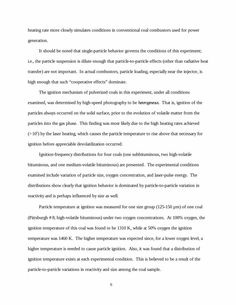
The ignition mechanism of pulverized coals in this experiment, under all conditions
examined, was determined by high-speed photography to be heterogeneous. That is, ignition of the
particles always occurred on the solid surface, prior to the evolution of volatile matter from the
particles into the gas phase. This finding was most likely due to the high heating rates achieved
(>105) by the laser heating, which causes the particle temperature to rise above that necessary for
ignition before appreciable devolatilization occurred.
Ignition-frequency distributions for four coals (one subbituminous, two high-volatile
bituminous, and one medium-volatile bituminous) are presented. The experimental conditions
examined include variation of particle size, oxygen concentration, and laser-pulse energy. The
distributions show clearly that ignition behavior is dominated by particle-to-particle variation in
reactivity and is perhaps influenced by size as well.
Particle temperature at ignition was measured for one size group (125-150 µm) of one coal
(Pittsburgh #8, high-volatile bituminous) under two oxygen concentrations. At 100% oxygen, the
ignition temperature of this coal was found to be 1310 K, while at 50% oxygen the ignition
temperature was 1460 K. The higher temperature was expected since, for a lower oxygen level, a
higher temperature is needed to cause particle ignition. Also, it was found that a distribution of
ignition temperature exists at each experimental condition. This is believed to be a result of the
particle-to-particle variations in reactivity and size among the coal sample.

7
The measured ignition temperatures were analyzed using the Distributed Activation Energy
Model of Ignition, and the ignition rate constant was determined to have an average value of 73
kJ/mol with a standard deviation of 3.7 kJ/mol. It is imperative to collect an extensive set of
ignition data in order to establish meaningful statistics for the extraction of ignition rate constants.
We plan to continue this study and to collect the data just described. Additionally, we make an
extensive set of recommendations for future work.

8
Introduction
Over the last several decades many experiments have been conceived to study the ignition of
pulverized coal and other solid fuels. We constructed a laser-based apparatus that offers several
advantages over those currently in favor. Sieve-sized particles are dropped batch-wise into a
laminar, upward-flow wind tunnel that is constructed with a quartz test section. The gas stream is
not preheated. A single pulse from a Nd:YAG laser is focused through the tunnel and ignites
several particles. The transparent test section and cool walls allow for application of two-color
pyrometry to measure the particles’ temperature history during ignition and combustion. Coals
ranging in rank from lignites to low-volatile bituminous, and chars derived from these coals, will be
studied in this project. For each fuel type, measurements of the ignition temperature under various
experimental conditions (particle size and free-stream oxygen concentration), combined with a
detailed analysis of the ignition process, will permit the determination of kinetic rate constants of
ignition.
This technique offers many advantages over conventional drop-tube furnace experiments.
One is the ability to directly measure ignition temperature rather than inferring it from
measurements of the minimum gas temperature needed to induce ignition. Another advantage is the
high heating rates achievable — on the order of 106 K/s. This is a significant improvement over
experiments which rely on convective heating from a hot gas, which typically achieves heating rates
of 104 K/s. The higher heating rate more closely simulates conditions in conventional coal
combustors used for power generation.
It should be noted that single-particle behavior governs the conditions of this experiment;
i.e., the particle suspension is dilute enough that particle-to-particle effects (other than radiative heat
transfer) are not important. In actual combustors, particle loading, especially near the injector, is
high enough that such “cooperative effects” dominate. Our approach is to gain a clear

9
understanding of single-particle behavior with this experiment, before facing the more difficult
problem encountered with cloud suspensions.
Our main motivations for this project are to determine the ignition mechanism of various
coals and to measure the ignition rate constant of a range of coals under single-particle conditions.
Our long-range, ultimate objectives are to (1) describe the ignition behavior of coals in a
suspension, (2) predict the ignition behavior of blend(s) of coals in a suspension, and (3) apply these
predictive tools in the design of burners and boiler units.

10
Objectives
Our specific, overall objectives for this project are:
1. Construction of the laser-ignition experiment, including:
1.1. gas delivery and regulation system;
1.2. wind tunnel;
1.3. exhaust system;
1.4. laser system and beam-guiding optics;
1.5. optical detection system; and
1.6. data acquisition and processing;
2. Shakedown testing of the various components;
3. Ignition of coals of various rank, from lignites to low-volatile bituminous;
4. Measurement of the ignition temperatures of these fuels under various experimental conditions
(particle size and free-stream oxygen concentration);
5. Extraction of ignition rate constants from temperature measurements by application of an
appropriate heterogeneous-ignition analysis.

11
Results and Discussion
I. Experiment Development
A. Experiment Overview
Figure 1 presents a schematic of the laser ignition experiment; the inset shows the details
around the test section. Sieve-sized particles were dropped through a tube into a laminar, upward-
flow wind tunnel with a quartz test section (5 cm square cross-section). The gas was not preheated.
The gas flow rate was set so that the particles emerged from the feeder tube, fell approximately 5
cm, then turned and traveled upward out of the tunnel. This ensured that the particles were
moving slowly downward at the ignition point, chosen to be 3 cm below the feeder-tube exit. A
single pulse from a Nd:YAG laser was focused through the test section, then defocused after
exiting the test section, and two addition prisms folded the beam back through the ignition point.
Heating the particles from two sides in this manner achieved more spatial uniformity and allowed
for higher energy input than a single laser pass. For nearly every case, two to five particles were
contained in the volume formed by the two intersecting beams, as determined by observation with
high-speed video.
The laser operated at 10 Hz and emitted a nearly collimated beam (6 mm diameter) in the
near-infrared (1.06 µm wavelength). The laser pulse duration was ~100 µs and the pulse energy was
fixed at 830 mJ per pulse, with pulse-to-pulse energy fluctuations of less than 3%. The laser pulse
energy delivered to the test section was varied by a polarizer placed outside of the laser head;
variation from 150 to 750 mJ was achieved by rotating the polarizer. Increases in the laser pulse
energy resulted in heating of the coal particles to higher temperatures. At the ignition point the
beam diameter normal to its propagation direction was ~3 mm on each pass of the beam. An air-
piston-driven laser gate (see Figure 1) permitted the passage of a single pulse to the test section.

12
The system allowed for control of the delay time between the firing of feeder and the passage of
the laser pulse, which was necessary since coal samples of different sizes and/or densities required
different time periods to fall through the feeder tube. Finally, ignition or nonignition was
determined by examining the signal generated by a high-speed silicon photodiode connected to a
digital oscilloscope.
flowconditioning
section
O2/N2
lens
quartztest
sectionprism
focusinglens
laserbeam
beamdump
O2/N2
detector /amplifier
oscilloscope
opticalfiber
defocusing lens
laser gate
Figure 1: Schematic showing the laser ignition apparatus.
B. Coal preparation and handling
Coals were received from Penn State Coal Sample Bank packed under an argon atmosphere.
Approximately 150 gm of coal was transferred into pint jars for vacuum drying at 10 in. Hg and
76oC for 8 hours. Each coal was then dry sieved and stored in small jars kept in desiccator cabinets.
13
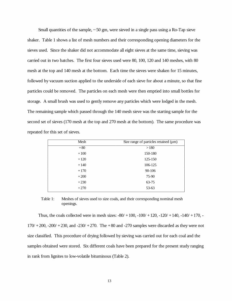
Small quantities of the sample, ~50 gm, were sieved in a single pass using a Ro-Tap sieve
shaker. Table 1 shows a list of mesh numbers and their corresponding opening diameters for the
sieves used. Since the shaker did not accommodate all eight sieves at the same time, sieving was
carried out in two batches. The first four sieves used were 80, 100, 120 and 140 meshes, with 80
mesh at the top and 140 mesh at the bottom. Each time the sieves were shaken for 15 minutes,
followed by vacuum suction applied to the underside of each sieve for about a minute, so that fine
particles could be removed. The particles on each mesh were then emptied into small bottles for
storage. A small brush was used to gently remove any particles which were lodged in the mesh.
The remaining sample which passed through the 140 mesh sieve was the starting sample for the
second set of sieves (170 mesh at the top and 270 mesh at the bottom). The same procedure was
repeated for this set of sieves.
Mesh Size range of particles retained (µm)
+80 >180
+100 150-180
+120 125-150
+140 106-125
+170 90-106
+200 75-90
+230 63-75
+270 53-63
Table 1: Meshes of sieves used to size coals, and their corresponding nominal meshopenings.
Thus, the coals collected were in mesh sizes: -80/+100, -100/+120, -120/+140, -140/+170, -
170/+200, -200/+230, and -230/+270. The +80 and -270 samples were discarded as they were not
size classified. This procedure of drying followed by sieving was carried out for each coal and the
samples obtained were stored. Six different coals have been prepared for the present study ranging
in rank from lignites to low-volatile bituminous (Table 2).

14
(Dry wt%) (Dry, Ash-Free wt%)Coal Type Volatile
MatterAsh C H N O+S
(diff)DECS 13
Sewellmvb
24.98 4.22 84.47 4.74 1.44 5.13
DECS 19Pocahontas
lvb18.31 4.60 85.74 4.67 1.09 3.90
DECS 23Pittsburgh
hvAb39.42 9.44 74.21 5.10 1.35 9.90
DECS 24Illinois #6
hvCb40.83 13.39 66.05 4.59 1.14 14.83
DECS 25Pust
lignite A41.98 11.85 65.76 4.60 0.94 16.85
DECS 26Wyodak
subbituminous44.86 7.59 69.77 5.65 0.94 16.07
Table 2: Proximate and ultimate analyses of coals used.
The coals were dried in a vacuum oven at 70oC for 24 h prior to use for each day’s
experiment(s). It is critically important to carefully control the contact between the dried coals and
any moisture – in the air and on the hands of handlers – in order to obtain good reproducibility of
data from day to day. For this reason, the coals were removed from the oven just prior to running
experiments each day, and only one batch was loaded into the coal feeder for each day’s use.
C. Gas-handling system
The gas flow system is shown in Figure 2. Oxygen and nitrogen were directed separately
through pressure regulators and flowmeters. The two gases were blended in the required ratio and
flow rates, and directed to the wind tunnel as a mixture. Figure 3 shows a photograph of the gas
flow system.

15
Flow Panel
Valves
Flowmeters
PressureRegulator
To wind tunnel
NitrogenOxygen
Figure 2: Schematic showing gas-handling system.
Figure 3: Photograph showing the gas-handling system.
16
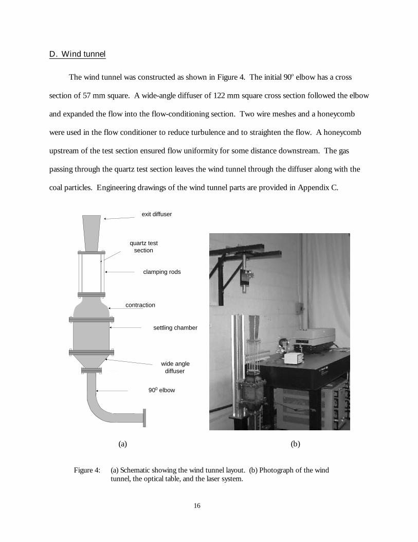
D. Wind tunnel
The wind tunnel was constructed as shown in Figure 4. The initial 90o elbow has a cross
section of 57 mm square. A wide-angle diffuser of 122 mm square cross section followed the elbow
and expanded the flow into the flow-conditioning section. Two wire meshes and a honeycomb
were used in the flow conditioner to reduce turbulence and to straighten the flow. A honeycomb
upstream of the test section ensured flow uniformity for some distance downstream. The gas
passing through the quartz test section leaves the wind tunnel through the diffuser along with the
coal particles. Engineering drawings of the wind tunnel parts are provided in Appendix C.
exit diffuser
quartz testsection
clamping rods
contraction
settling chamber
wide anglediffuser
900 elbow
(a) (b)
Figure 4: (a) Schematic showing the wind tunnel layout. (b) Photograph of the windtunnel, the optical table, and the laser system.

17
The feeder is a capped cylinder (12 mm ID) with a tapered bottom connected to a 4-mm
tube (Figure 5). Within the feeder a wire mesh was suspended; the mesh also acted as a support for
a mound of particles. A jolt to the feeder resulted in particles falling through the mesh and into the
feeder tube. A small air-driven piston, controlled electronically for timing purposes through a
solenoid valve, glanced the side of the feeder to provide the required jolt. The mesh used inside
should be larger than the finest through which the particles will pass, such that only a few hundreds
of particles fell for each run. Table 3 provides a list of meshes that were used for our experiments.
wire mesh
1/2" ID
1/8" OD tube
tapering section
Figure 5: Cross-sectional view of the coal feeder.
Particles Size (µm) Mesh Used in Feeder150-180125-150106-12563-75
607080100
Table 3: Particles sizes and corresponding mesh used in feeder.

18
E. Laser system and associated optics
The laser used was a Nd:YAG laser which operates at a pulse rate of 10 Hz and with a
maximum energy of 850 mJ in the primary (1064 nm) output. The pulse duration was 100 µs. At
the ignition point, the beam diameter normal to its direction of propagation was approximately
3 mm on each pass. The laser was triggered externally by a digital pulse generator; a second pulse
generator was synchronized with the first to control the delay time between firing of the feeder and
the laser gate, which determined the delay in the passage of the laser pulse through the test section.
The laser beam was focused through the tunnel using a convex lens (focal length 750 mm). It
was defocused upon leaving the test section using a concave lens (focal length 150 mm), and folded
back to the ignition point using two prisms. The use of two laser passes through the test section
achieved more spatial uniformity in heating the coal particles and allowed for higher energy input
than a single laser pass. The beam was finally stopped by a beam dump.
F. Experiment procedure
A typical run of our experiment is conducted as follows: The coal and oxygen concentration
were first chosen for study. The coal was then loaded into the feeder. The delay time between the
triggering of the feeder and the appearance of the coal sample at the feeder tube exit was visually
observed and timed with a stop watch; typical values were ~2.3-2.9 s. The gas flow rate required to
ensure that particles move slowly upward at the point of ignition was determined by visual
observation during this time as well. The digital pulse generator was then programmed for the
delay time to trigger the laser gate. Next, a laser pulse energy was set. At each laser pulse energy, 20
attempts at ignition were made in order to measure the ignition frequency or probability, which is
the parameter sought from these studies. A digital storage oscilloscope recorded the signal from
the detector, which determined whether or not particle(s) ignited on each attempt. The experiment

19
was repeated over a range of laser pulse energies to produce a laser energy versus ignition frequency
plot, which we refer to as an ignition distribution. Detailed, step-by-step procedure of the conduct
of each day’s experiment is provided in Appendix D.
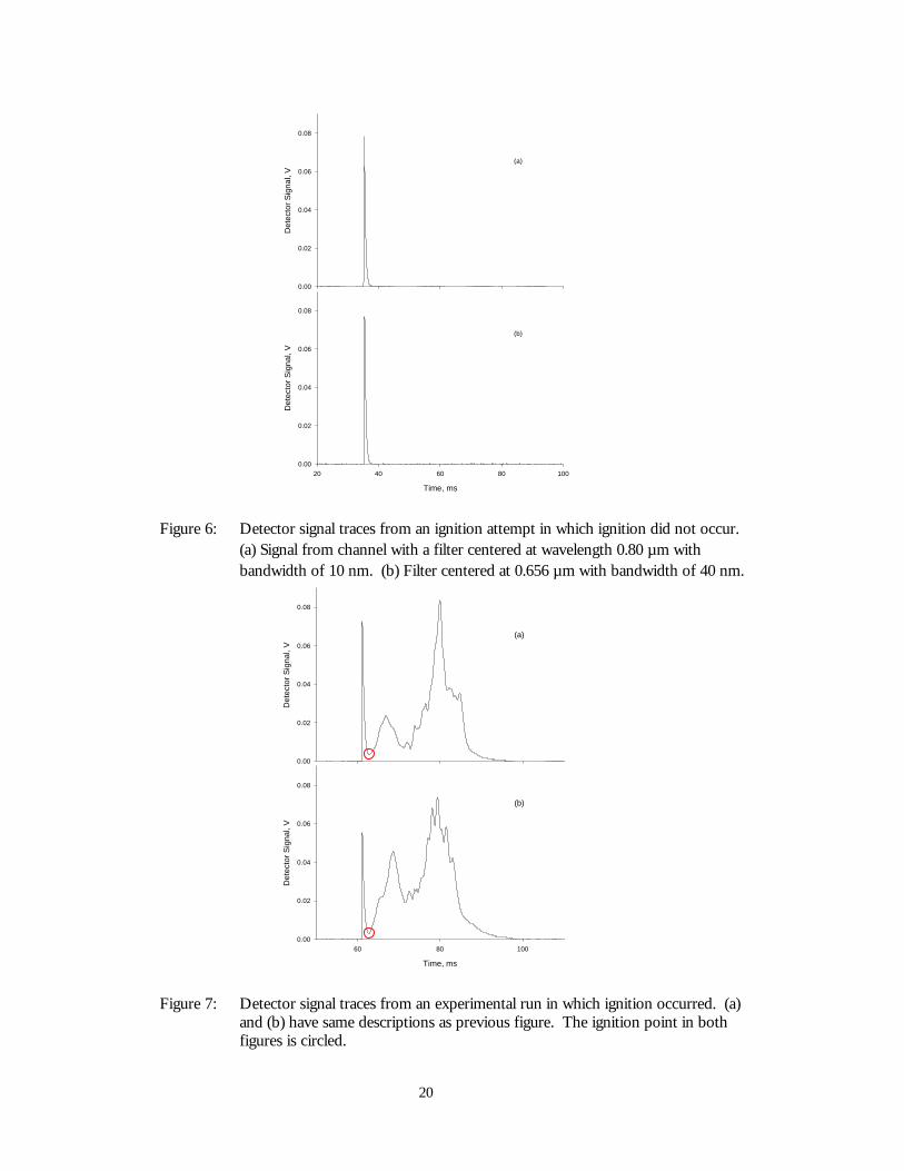
Figure 6 shows a pair of detector signals from a experimental run in which ignition did not
occur. The sharp spike observed by the detectors arise from the rapid heating caused by the laser
pulse, and the cooling due to radiative and convective losses from the particle surface, as we have
shown previously [4]. Figure 7 shows the same two detectors observing a run in which ignition
does occur. The signals are dramatically different due to the ignition and subsequent combustion.
Both traces still show the initial spike, due to laser-induced heating followed by surface cooling. In
this case, however, the temperature to which the particle(s) equilibrated was at or above that
necessary for ignition. As we have shown previously, the particles ignite heterogeneously on the
solid particle surface prior to any evident expulsion of volatile matter.
The ignition traces also show the characteristic two-pulse combustion behavior we observed
previously in a similar experiment [4]. The two pulses following the initial spike were observed by
high-speed video to be due to the consecutive evolution and combustion of volatile matter ejected
from the particle. This combustion behavior is observed consistently in every ignited experimental
run when testing with subbituminous and high-volatile bituminous coal. We hypothesized in the
referenced article that the two successive pulses of volatile matters are due to the evolution of tar
and oils, followed by combustible light gases (CH4, H2, CO). Of course, for this study, we are
interested in mainly the ignition process, thus our measurements focus only on the point in time
circled in Fig. 7, which corresponds to the ignition point. The measurement of the particle
temperature at ignition, and its use in extracting ignition rate constants are described in sections
I.G, IV, and V.
20
Det
ecto
r S
igna
l, V
0.00
0.02
0.04
0.06
0.08
Time, ms
20 40 60 80 100
Det
ecto
r S
igna
l, V
0.00
0.02
0.04
0.06
0.08
(a)
(b)
Figure 6: Detector signal traces from an ignition attempt in which ignition did not occur.(a) Signal from channel with a filter centered at wavelength 0.80 µm withbandwidth of 10 nm. (b) Filter centered at 0.656 µm with bandwidth of 40 nm.
60 80 100
Det
ecto
r S
igna
l, V
0.00
0.02
0.04
0.06
0.08
Time, ms
60 80 100
Det
ecto
r S
igna
l, V
0.00
0.02
0.04
0.06
0.08
(a)
(b)
Figure 7: Detector signal traces from an experimental run in which ignition occurred. (a)and (b) have same descriptions as previous figure. The ignition point in bothfigures is circled.

21
G. Two-color pyrometry system
1. Theory of Operation
This section describes the operational principles and expected performance of a two-
wavelength pyrometer used for particle-temperature measurement. The specific application in this
instance is the measurement of pulverized coal temperatures at ignition in an experiment where one
to five particles are ignited by a high-energy laser pulse. The light emitted by the igniting particles is
collected by a train of optics, divided into two or three light paths via a trifurcated optical-fiber
bundle, passed through a narrow bandpass interference filter, and finally detected by a
photomultiplier tube (PMT). Here we will examine the expected signal levels at the pyrometer, and
gauge the instrument’s temperature-measurement sensitivity.
We will assume coal particles to be gray, and thus emit light according to Planck’s blackbody
spectral distribution, modified by its coefficient of emissivity:
( ) ,
1T
Cexp
CTE
25
1
−
λλ
ε=λ (1)
where ε is the coal emissivity, λ is the wavelength, and T is the particle temperature. C1 and C2 are
the usual constants for Planck’s spectral distribution.
A very good approximation (<1% error at all wavelengths) to Planck’s distribution is:
( ) ,TC
expC
TE 2
5
1
λ−
λε
≈λ (2)
and we will make use of this approximation for the remainder of this paper. The units of Eq. (1) or
(2) are
µ⋅ mm
W2
, since each describes the power emitted by a gray body, per surface area, within
an infinitesimally small wavelength interval.

22
A two-wavelength, or two-color, pyrometer works on the principle that the temperature of a
gray surface or a blackbody can be determined simply by measuring the light (power) emitted by
that surface at two separate but known wavelengths. This principle is easily verified by examining Eq.
(2), in which the variable, Eλ (which is measured in the experiment), is dependent on λ and on T.
Thus, if Eλ1 and Eλ2, which represent the power measured at wavelengths λ1 and λ2, respectively,
were measured, the ratio of the powers, Eλ1/Eλ2, would yield the single unknown, T:
.11
TC
expEE
21
2
5
1
2
2
1
λ
−λ
−
λλ
=λ
λ (3)
The importance of the assumption of blackbody or gray body (constant ε) is now obvious from
examining Eq. (3), where the ratio of emissivities at the two wavelengths is assumed to be unity.
The actual determination of the power emitted by the particles is complicated by the fact that
various optical components lie in the path between the particle and the detector, and that the
detector has variable response, depending on the wavelength of light falling on it. Nevertheless, the
general principle of operation of the two-color pyrometer is as described above.
We now develop a more rigorous expression of the power detected at the PMT in order to
determine the expected pyrometer performance. The intensity of light given off by a gray body at
temperature T is:
( ) [ ] .srmm
WTC
expC
TI2
2
5
1
⋅µ⋅=
λ−
πλε
=λ (4)
Note that the principal difference between Eq. (2) and (4) is that the latter is the power emitted by
a gray body, per unit surface area, per infinitesimally small wavelength interval, and per
infinitesimally small solid angle. These dependencies are shown schematically below.
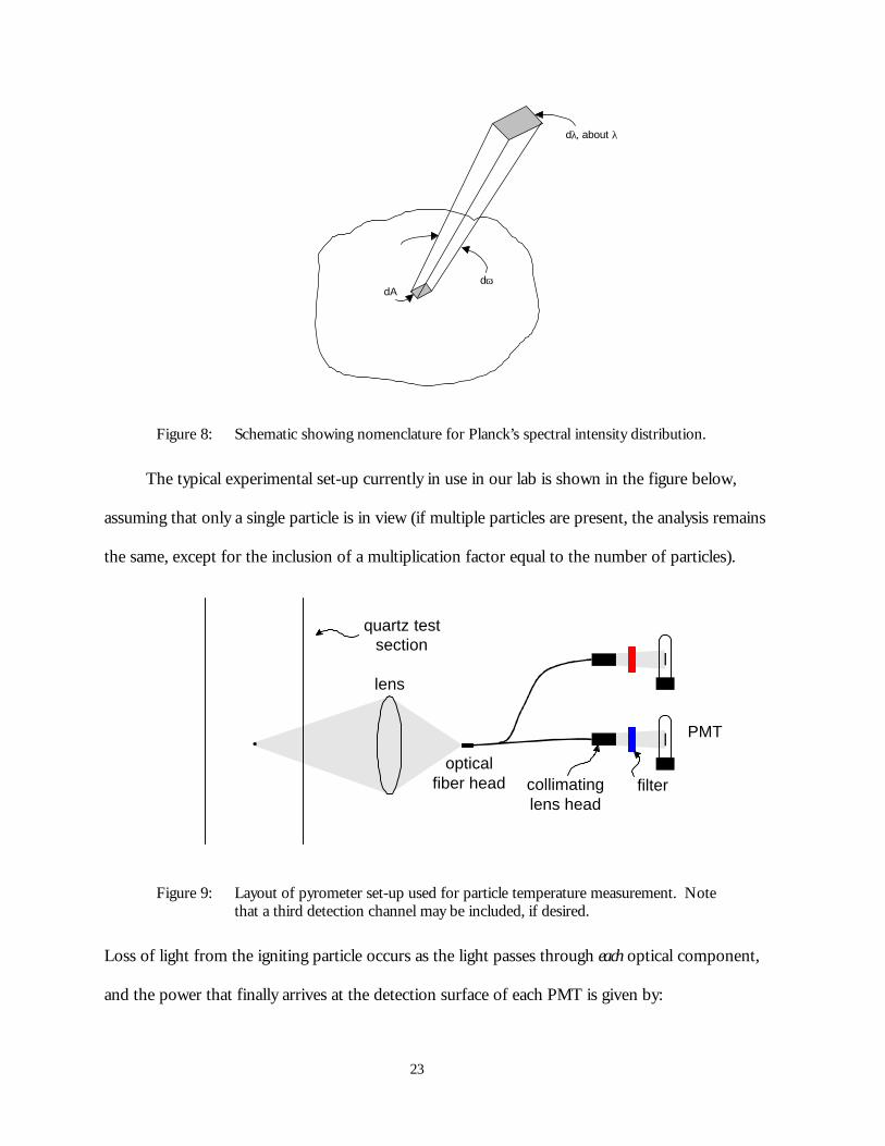
23
dAdω
dλ, about λ
Figure 8: Schematic showing nomenclature for Planck’s spectral intensity distribution.
The typical experimental set-up currently in use in our lab is shown in the figure below,
assuming that only a single particle is in view (if multiple particles are present, the analysis remains
the same, except for the inclusion of a multiplication factor equal to the number of particles).
quartz testsection
lens
opticalfiber head collimating
lens headfilter
PMT
Figure 9: Layout of pyrometer set-up used for particle temperature measurement. Notethat a third detection channel may be included, if desired.
Loss of light from the igniting particle occurs as the light passes through each optical component,
and the power that finally arrives at the detection surface of each PMT is given by:

24
[ ][ ]
[ ] .W A)T(I
ATC
expC
P
loss
windowPMTfilter
headlens
fiberopticallens
tionsectest
2
5
1
=τ⋅λ∆⋅Ω⋅=
ττττττλ∆Ω
λ−
πλε
=
λ
(5)
In words, the power that arrives at the PMT detection surface is simply the gray body’s emitted
intensity (Iλ), times the area-solid angle factor (AΩ, or etendue), times the spectral bandwidth of the
filter (∆λ), and finally multiplied by a factor which accounts for all the transmission losses due the
optical components in the system. In the expression for P, Iλ depends on the particle temperature
(which is what we seek) and the wavelength of the chosen filter, ∆λ depends on the optical
bandwidth (FWHM) of the filter, and both the etendue and τlosses depend on the optical system.
Note, however, that all three factors are fixed, and do not change from run to run, so long as the
optical system and filters do not change. While Eq. (5) can be used to calculate the power detected
by the PMT, and can even be used to determine the particle temperature in a single-color
pyrometer, the solution is highly uncertain due mainly to the uncertainties in the particle emissivity,
the etendue, and the various transmission losses. This uncertainty is the reason that two-color
pyrometers are more favored.
To complete this analysis, the signal (S), as an electrical current, developed by the PMT is
simply:
λλ ⋅τ⋅λ∆⋅Ω⋅= RA)T(IS loss (6)
where S has units of amps (A). Rλ is referred to as the PMT’s responsivity, and has units of A/W.
(The subscript on responsivity is a reminder that this value is a function of the wavelength of light
that strikes it.) Input of this current into an appropriate current-to-voltage converter will then
produce a voltage for detection.
Starting with Eq. (6), it is now possible to develop an expression for the ratio of two signals
from a two-color pyrometer:
25
τ
τ
λ∆λ∆
=
λ
λ
λ
λ
2
1
2,loss
1,loss
2
1
2
1
2
1
RR
II
SS
, (7)
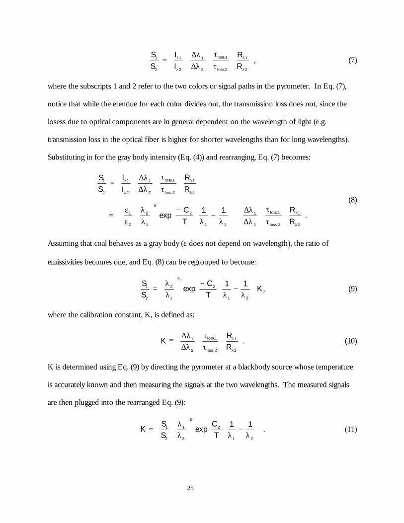
where the subscripts 1 and 2 refer to the two colors or signal paths in the pyrometer. In Eq. (7),
notice that while the etendue for each color divides out, the transmission loss does not, since the
losess due to optical components are in general dependent on the wavelength of light (e.g.
transmission loss in the optical fiber is higher for shorter wavelengths than for long wavelengths).
Substituting in for the gray body intensity (Eq. (4)) and rearranging, Eq. (7) becomes:
.R
R11T
Cexp
R
R
I
I
SS
2
1
2,loss
1,loss
2
1
21
2
5
1
2
2
1
2
1
2,loss
1,loss
2
1
2
1
2
1
τ
τ
λ∆λ∆
λ
−λ
−
λλ
εε
=
τ
τ
λ∆λ∆
=
λ
λ
λ
λ
λ
λ
(8)
Assuming that coal behaves as a gray body (ε does not depend on wavelength), the ratio of
emissivities becomes one, and Eq. (8) can be regrouped to become:
K11
TC
expSS
21
2
5
1
2
2
1
λ
−λ
−
λλ
= , (9)
where the calibration constant, K, is defined as:
ττ
λ∆λ∆
≡λ
λ
2
1
2,loss
1,loss
2
1
RR
K . (10)
K is determined using Eq. (9) by directing the pyrometer at a blackbody source whose temperature
is accurately known and then measuring the signals at the two wavelengths. The measured signals
are then plugged into the rearranged Eq. (9):
λ
−λ
λλ
=
21
2
5
2
1
2
1 11T
Cexp
SS
K . (11)
26
This calibration eliminates the need to know accurately the transmission losses, filter bandwidths,
and PMT responsivities, and is the main reason that two-color pyrometers are more often used
than single-color pyrometers.
Once K is determined from calibration, the pyrometer is ready for use to measure particle
temperatures. Directing the pyrometer now at igniting coal particles and measuring the signals, S1
and S2, these values can then be substituted into the following equation, which is simply a
rearrangement of Eq. (9), in order to determine the particle temperature:
λλ
λ
−λ
−=
5
2
1
2
1
21
2
SS
K1
ln
11C
T . (12)
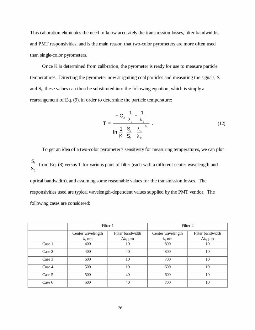
To get an idea of a two-color pyrometer’s sensitivity for measuring temperatures, we can plot
2
1
S
S from Eq. (8) versus T for various pairs of filter (each with a different center wavelength and
optical bandwidth), and assuming some reasonable values for the transmission losses. The
responsivities used are typical wavelength-dependent values supplied by the PMT vendor. The
following cases are considered:
Filter 1 Filter 2
Center wavelengthλ, nm
Filter bandwidth∆λ, µm
Center wavelengthλ, nm
Filter bandwidth∆λ, µm
Case 1 400 10 800 10
Case 2 400 40 800 10
Case 3 600 10 700 10
Case 4 500 10 600 10
Case 5 500 40 600 10
Case 6 500 40 700 10
27
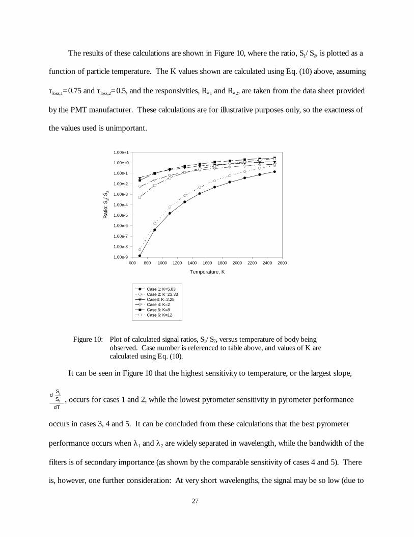
The results of these calculations are shown in Figure 10, where the ratio, S1/S2, is plotted as a
function of particle temperature. The K values shown are calculated using Eq. (10) above, assuming
τloss,1=0.75 and τloss,2=0.5, and the responsivities, Rλ1 and Rλ2, are taken from the data sheet provided
by the PMT manufacturer. These calculations are for illustrative purposes only, so the exactness of
the values used is unimportant.
Temperature, K
600 800 1000 1200 1400 1600 1800 2000 2200 2400 2600
Rat
io: S
1/ S
2
1.00e-9
1.00e-8
1.00e-7
1.00e-6
1.00e-5
1.00e-4
1.00e-3
1.00e-2
1.00e-1
1.00e+0
1.00e+1
Case 1: K=5.83 Case 2: K=23.33 Case3: K=2.25 Case 4: K=2 Case 5: K=8 Case 6: K=12
Figure 10: Plot of calculated signal ratios, S1/S2, versus temperature of body beingobserved. Case number is referenced to table above, and values of K arecalculated using Eq. (10).
It can be seen in Figure 10 that the highest sensitivity to temperature, or the largest slope,
dT
S
Sd
2
1
, occurs for cases 1 and 2, while the lowest pyrometer sensitivity in pyrometer performance
occurs in cases 3, 4 and 5. It can be concluded from these calculations that the best pyrometer
performance occurs when λ1 and λ2 are widely separated in wavelength, while the bandwidth of the
filters is of secondary importance (as shown by the comparable sensitivity of cases 4 and 5). There
is, however, one further consideration: At very short wavelengths, the signal may be so low (due to

28
the nature of Planck’s blackbody distribution function and the low PMT responsivity) that it is at a
level near or below the noise level. Thus, while the goal should be to maximize the separation of
the two wavelengths of the filters chosen for the pyrometer, the lower wavelength is also limited by
the detection limit set by the signal-to-noise ratio. These observations can be confirmed by taking
the derivative of S1/S2 (Eq. (9)) with respect to T.
2. System Design
The layout of the pyrometry and photography system is shown in Figure 11. The receiving
optics (lens and optical fiber bundle) of the pyrometer is shown to the right of the test section, and
the calibration source is to the left. The path of the calibration beam is shaded in gray while the
path of the light captured by the receiving optics is outlined only. The outline is present on the
region between the center of the test section and the achromat lens to denote that the two lenses
have been matched to capture the same solid angle. This point will be explained in detail later. The
high-speed camera system is shown in its position above the receiving optics, and viewing the
ignition point in the test section at an angle through a chopper wheel.
blackbodysource
achromatlens (f1, D1) simple
lens (f2, D2)
opticalfiber bundle
quartz testsection chopper
wheel
SLR camera withtelephoto lens
s2's2s1's1
Figure 11: Schematic showing layout of pyrometry system relative to experiment, includingreceiving optics, calibration (blackbody) source, and high-speed photographysystem.

29
The starting point for the design of the optical system is the constraint that we will be dealing
with extremely low light levels – as low as the light emitted by a single 100-µm coal particle at
500oC. Thus, the need to maximize the amount of light that is collected by the receiving, or
detection, optics, drives our system design. The fiber-optic bundle can receive light input at a
maximum total angle of 68o; no standard lens is this fast. Our system therefore will be limited by
the “speed” of the simple lens, and we simply choose the “fastest” (lowest f/D, or focal length-to-
diameter ratio) lens we can find. For our system, we’ve chosen an f=62.9 mm/D=50.8 mm lens,
giving a f/D of 1.23.
To determine the location of the receiving lens, we consider that the diameter of the fiber-
optic bundle is 5.5 mm, which is approximately one-half the diameter of the area from which we
want to detect igniting particles. We make this choice even though the actual ignition point is only
~2-3 mm in diameter in order to give a margin of error for alignment and for particle motion. This
choice of detection area means that we want 2:1 imaging, or a magnification of 0.5. With this
constraint we can now calculate the distances s2 and s2’ shown in Figure 11. The lens equation is:
2'22 f
1s1
s1
=+ , (13)
which relates the object distance (s2), the image distance (s2’), and the focal length of the lens. The
additional constraint is the magnification (M) of 0.5:
5.0ss
M2
'2 == . (14)
Substituting Eq. 14 into Eq. 13, we find that for 2:1 imaging:
,f3s2
and ,s2s
'2
'22
=
=
and using f2=62.9 mm in this case gives s2’=94.4 mm (3.7 in.) and s2=188.7 mm (7.4 in.).

30
We now move to the specification of the optics for the calibration source. Here we have two
considerations: (1) the need to match the solid angle subtended by the receiving optics to the image
of the calibration source, as shown in Figure 11 (that is, we want to fill the receiving lens with the
light from the calibration source, just as igniting particles would); and (2) the desired
demagnification of the calibration source, which is a 1-mm diameter blackbody source.
To satisfy the first consideration, we want to match the angles, α1 and α2, shown in Figure 12.
The two lenses have different diameters, and to match the angles, we simply note the similar angles:
Ds
Ds
2
2
1
'1
21
=
α=α
s2 and D2 are set from our previous consideration, and we choose D1 to be 25 mm, since a fast
achromat lens is much more widely available in this size than in the 50 mm version. (The need for
an achromat lens is explained later.) This choice results in s1’=92.9 mm (3.7 in.).
blackbodysource
achromatlens (f1, D1) simple
lens (f2, D2)
opticalfiber bundle
α 1 α 2
Figure 12: Schematic showing the angles subtended by the calibration-source imagingoptics, and the receiving optics.
The second consideration involves the chosen demagnification of the calibration source. The
coals we will use are in the size range of 60-200 µm diameter, and the blackbody source is 1 mm in

31
diameter. Thus, a demagnification factor of 3 to 10 (M=1/3 to 1/10) is desired to simulate the
possible range of particle size and numbers we might encounter in the experiment. To specify the
lenses’ focal length and s1, we again apply the lens equation and the definition of magnification:
1
'1
ss
M =
1'11 f
1s1
s1
=+
These two equations can be solved simultaneously for the two unknowns, s1 and f1; the solutions
are shown in Table 4.
s1' = 92.9
M f1 f1 (in.) s1 s1 (in.)
0.333333 69.7 2.7 278.7 11.00.25 74.3 2.9 371.6 14.60.2 77.4 3.0 464.5 18.3
0.166667 79.6 3.1 557.4 21.90.142857 81.3 3.2 650.3 25.6
0.125 82.6 3.3 743.2 29.30.111111 83.6 3.3 836.1 32.9
0.1 84.5 3.3 929.0 36.6
Table 4: Calculation of focal length, f1, and image distance, s1, for the calibration source.All units are in mm unless noted otherwise.
Our final lens selection for the calibration source is dictated by the available achromat lenses,
and the reasonableness of the required s1, which is excessive in some instances. An f=75 mm
achromat lens is available, so our calibration optics will have these final characteristics:
D1 = 25 mm
f1 = 75 mm
s1’ = 92.9 mm (3.7 in.)
32
s1 = 389.2 mm (15.3 in.)
M = 1/4.2
The 1-mm diameter calibration source will be projected into the test section to an image size of
238 µm (1 mm/4.2).
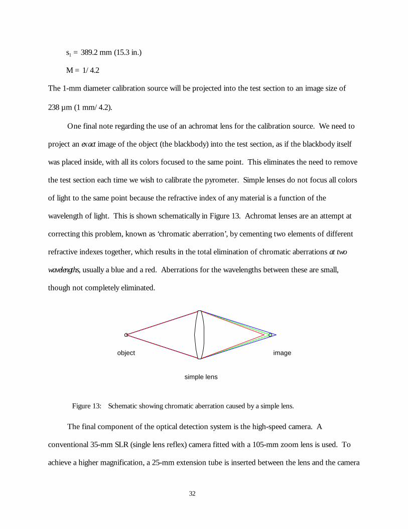
One final note regarding the use of an achromat lens for the calibration source. We need to
project an exact image of the object (the blackbody) into the test section, as if the blackbody itself
was placed inside, with all its colors focused to the same point. This eliminates the need to remove
the test section each time we wish to calibrate the pyrometer. Simple lenses do not focus all colors
of light to the same point because the refractive index of any material is a function of the
wavelength of light. This is shown schematically in Figure 13. Achromat lenses are an attempt at
correcting this problem, known as ‘chromatic aberration’, by cementing two elements of different
refractive indexes together, which results in the total elimination of chromatic aberrations at two
wavelengths, usually a blue and a red. Aberrations for the wavelengths between these are small,
though not completely eliminated.
object
simple lens
image
Figure 13: Schematic showing chromatic aberration caused by a simple lens.
The final component of the optical detection system is the high-speed camera. A
conventional 35-mm SLR (single lens reflex) camera fitted with a 105-mm zoom lens is used. To
achieve a higher magnification, a 25-mm extension tube is inserted between the lens and the camera
33
body. The camera is operated in the manual mode with the shutter held open and all room lighting
eliminated. The light emitted by the igniting and burning particles will thus be captured. To
produce discrete images on the high-sensitivity black-and-white film, a chopper wheel is placed in
front of the camera lens to provide ‘shuttering’ at approximate 500 Hz. Thus, one image will be
recorded roughly every 2 ms of experiment time until the igniting particles leave the camera’s field
of view.
3. Calibration Procedure
The goal of the calibration is to determine the calibration constant, K, of Eq. (10). Since it is not
practicable to measure each variable of Eq. (10), it is simpler and more straightforward to measure
this parameter by directing the pyrometer at a blackbody source whose temperature is accurately
known and then measuring the signals at the two wavelengths for various temperatures. The
measured signals are then substituted into Eq. (11) and K is found by a ‘best fit’ through the data
points.
This calibration eliminates the need to know accurately the transmission losses, filter
bandwidths, and PMT responsivities, and is the main reason that two-color pyrometers are more
often used than single-color pyrometers. Furthermore, it should be noted the although
measurements of PMT signal are made at several temperatures, the pyrometer actually requires only
a single-point calibration, which means the procedure is both fast and simple.
II. Data Reduction Methodology
The measured particle temperatures at ignition is analyzed to extract the ignition rate constant
by application of the Distributed Activation Energy Model of Ignition (DAEMI), which we first
developed to interpret results from conventional, drop-tube, ignition experiments (see description

34
below and the reprint of the publication in Appendix A). The model has been modified from its
original form for application to this project as described below.
Numerous experiments have been conducted over the past three decades to measure the
ignition rates of pulverized coals. Most of these are reviewed by Essenhigh et al. [1], and the most
popular method is described next. In order to extract rate constants from any ignition experiment,
it is necessary to apply a model of the ignition process to analyze the data, which usually consists of
some readily measurable parameter such as the gas temperature necessary to cause ignition. What
all previous experiments have in common is that within each model, ignition is represented by a
single Arrhenius rate constant, which of course represents some average value for the coal particles within
that sample. This method is chosen for convenience but does not accurately represent the reality,
since it is well established – from single particle experiments [2] – that for coals of the same type
and size, particle-to-particle variations exist. These variations include size, density, mineral-matter
content, specific heat and, most importantly, chemical reactivity. Thus, our goal in this phase of
study is to develop a model of coal ignition which accounts for the variation in reactivity, and to
apply it to our data in order to extract more meaningful ignition rate constants.
Recently, we presented a model of heterogeneous coal ignition which accounts for particle-
to-particle variation in reactivity within a sample, and showed that it correctly depicts, for the first
time, all key observations from conventional drop-tube furnace experiments [3]. The Distributed
Activation Energy Model of Ignition (DAEMI) accounts for the variation in reactivity by including
a single preexponential factor, as usual, and a Gaussian distribution of activation energies among the
particles to describe their ignition kinetics. This distribution provides the particle-to-particle
variation in reactivity we seek to inject into our model. By adjusting the parameters in the model,
main characteristics of experimental results were captured, namely (1) the gradual increase in
35
ignition frequency with increasing gas temperature, and (2) the variation of the slope of the ignition
frequency with oxygen concentration.
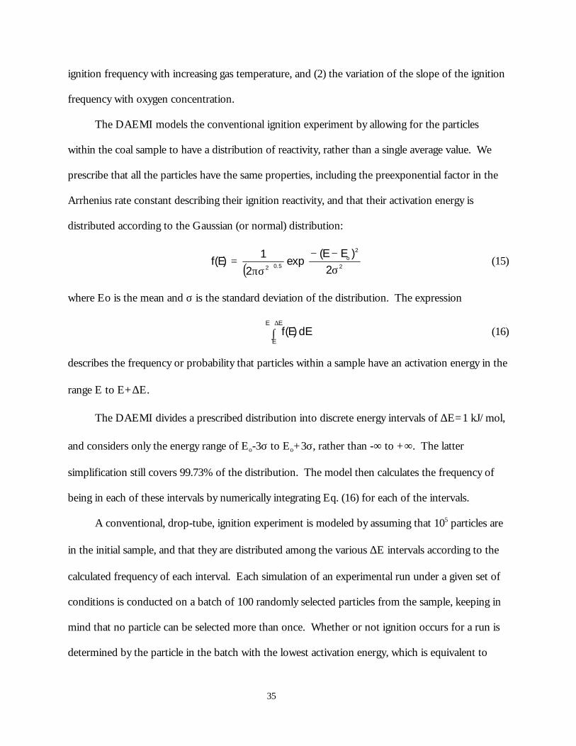
The DAEMI models the conventional ignition experiment by allowing for the particles
within the coal sample to have a distribution of reactivity, rather than a single average value. We
prescribe that all the particles have the same properties, including the preexponential factor in the
Arrhenius rate constant describing their ignition reactivity, and that their activation energy is
distributed according to the Gaussian (or normal) distribution:
( )
σ−−
πσ=
2
2o
5.02 2)EE(
exp2
1)E(f (15)
where Eo is the mean and σ is the standard deviation of the distribution. The expression
∫∆+ EE
EdE )E(f (16)
describes the frequency or probability that particles within a sample have an activation energy in the
range E to E+∆E.
The DAEMI divides a prescribed distribution into discrete energy intervals of ∆E=1 kJ/mol,
and considers only the energy range of Eo-3σ to Eo+3σ, rather than -∞ to +∞. The latter
simplification still covers 99.73% of the distribution. The model then calculates the frequency of
being in each of these intervals by numerically integrating Eq. (16) for each of the intervals.
A conventional, drop-tube, ignition experiment is modeled by assuming that 105 particles are
in the initial sample, and that they are distributed among the various ∆E intervals according to the
calculated frequency of each interval. Each simulation of an experimental run under a given set of
conditions is conducted on a batch of 100 randomly selected particles from the sample, keeping in
mind that no particle can be selected more than once. Whether or not ignition occurs for a run is
determined by the particle in the batch with the lowest activation energy, which is equivalent to

36
being the most reactive particle. If this particle’s reactivity equals or exceeds that determined by the
critical ignition condition, the batch is defined to be ignited. This is consistent with our observation
[4] that single-particle ignition is discernible to the eye. This procedure is repeated 20 times at each
condition, just as in actual experiments, to determine an ignition frequency at this condition.
Finally, the gas temperature is varied several times and, each time, 20 runs are conducted.
Figure 14 shows an application of the DAEMI in modeling the ignition experiments of
Zhang et al. [5]. Linear regressions of the experimental data are shown in the figure as solid lines,
and the data points are from the model. Notice that the model correctly depicts the increase in
ignition frequency with increasing gas temperature (Tg), and it captures both the decrease in the
slope of the ignition frequency with decreasing oxygen concentration and the slow rate of the
slope’s decrease until very low oxygen concentrations. These results represent the first time that a
model has depicted ignition data with such accuracy.
The original DAEMI is modified for the present experiment as follows. The initial batch of
coal is assumed to contain 4×10⁵ particles; this number is arrived at by determining the approximate
weight of a sample and making an estimate of the number of particles assuming a spherical particle
of the average size. 1300 particles are then selected randomly and act as feed into the test section;
again, this number is arrived at by measurement and estimation. Three particles are further selected
randomly from these 1300 to be heated by the laser pulse, keeping in mind that no particle can be
selected twice.

37
0
25
50
75
100
0
25
50
75
100
0
25
50
75
100
Tg (K)600 700 800 900 1000
0
25
50
75
100
Igni
tion
Freq
uenc
y (%
)
100% O2
50% O2
20% O2
10% O2
Figure 14: Linear regressions of experimental data from Ref. [5] (shown as solid lines),showing the effect of free-stream oxygen concentration on ignition of a high-volatile bituminous coal of 75-90 µm in diameter. The data points representresults from the DAEMI.
The heat generated, per unit surface are (S), by a spherical carbon particle undergoing
oxidation on its external surface may be given by the kinetic expression:
−=
p
inOc
G
RTE
expAphS
H2
(17)
Similarly, the heat loss from the surface of a particle at temperature Tp is the sum of losses due to
convection and radiation. Thus, heat loss from the surface may be given as:
( ) ( )4g
4pbgp
L TTTThS
H−εσ+−= (18)

38
At the non-critical condition of ignition (as is applicable to our experiment), the following
condition is satisfied:
LG HH > (19)
Thus, equating HG and HL and solving for E from Eq. (17) (assuming Nu=2 as is appropriate for
very small particles), we obtain [3]:
( ) ( )
−εσ+−
−=o
ngc
4g
4pbgp
p
g
p Aph
TTTTd
k2
lnRTE (20)
where the required parameters for this equation were calculated as follows:
1. Tp is determined by direct measurement from the two-color pyrometer, as described in
the previously in section I.G.
2. kg, the gas thermal conductivity in the boundary layer around a heated particle is given by
a linear fit to the conductivity of air determined at the average temperature of the particle
surface and gas:
+×=
2
TT100.7k gp5
g (21)
3. Ao, the preexponential factor was arbitrarily chosen as 250 kg m-2 s-1.
4. n, the reaction order is assumed to be 1.
5. ε, the emissivity of coal particles is chosen to be 0.8
6. hc is defined by the equation
2CO,CCO,Cc 'H1y
1'H
1yy
h+
++
= (22)

39
where ymol CO
mol CO=
2
was obtained from the equation [3]:
−=
p2 T3214
exp95.59COmolCOmol
(23)
H C CO' , and H C CO' , 2 are the heats of combustion corresponding to the following
oxidation reactions:
CkgkJ
790,32'H;COOC
CkgkJ
210,9'H;COO21
C
2CO,C22
CO,C2
=→+
=→+
(24)
Twenty runs were made at each laser energy to obtain ignition-frequency distributions.
Detailed simulation results are provided in the following section. Although it was assumed that
pulverized-coal ignition occurs heterogeneously without influence from any volatile matter that may
be present, and even though the results closely fit the experimental data, DAEMI does not confirm
that ignition is purely a heterogeneous process. Very few models of homogeneous ignition have
been developed, and none have been tested against the available experimental data because of the
inherent difficulty and uncertainty in modeling devolatilization and the combined solid-gas and gas-
gas reactions.
III. Ignition-Frequency Distribution Data
The present study provides ignition frequency as a function of oxygen concentration,
particle diameter and coal type. We have examined three sizes of four coals under three oxygen
concentrations. At each set of conditions (coal type, size and oxygen concentration), the ignition
frequency was measured over a range of laser pulse energy values. Twenty attempts at ignition were
made at each laser pulse energy to determine the frequency, or probability, of ignition. The
frequency thus obtained was mapped against the corresponding laser energies for these coals as

40
ignition-frequency distributions, and are presented below organized by coal type. The experimental
data has been provided in tabular numerical format in Appendix D.
Pittsburgh # 8 – high-volatile A bituminous
Figure 15 shows the ignition-frequency distributions for the 165 µm (150-180 µm range)
high-volatile A bituminous Pittsburgh #8 coal at various oxygen concentrations. It can be seen that
at each oxygen concentration, the ignition frequency increases approximately linearly over a range
of laser pulse energy. At each oxygen concentration, there is a lower laser energy below which the
probability of ignition is zero, and a higher energy above which there is 100% ignition probability.
The slope in frequency distribution is indicative of the variation of reactivity among the particles, as
described in the previous section on data reduction using the DAEMI.
The ignition frequency increases with increasing laser pulse energy since high pulse energy
translates to a higher particle temperature achieved. Thus, using the laser pulse to heat several
randomly chosen particles from the batch of particles dropped into the experiment, there is an
increasing probability that one of the heated particles will ignite as the particles are heated to higher
temperatures.
The shifting of the distributions to higher laser energies as oxygen concentration is decreased
is expected, since at lower oxygen levels, the amount of heat generated by the particle is decreased
(see Eq. (17)). Thus, in order to achieve a constant ignition frequency as oxygen concentration is
decreased, the particles must be heated initially to a higher temperature using higher laser energy.
The general observations described above applies to Figure 16 for the 116 µm Pittsburgh
coal, as well as to all coals studied under all conditions. The solid and open circles in Figure 16
represent the ignition frequencies obtained for 116 µm Pittsburgh coal at 100% oxygen
concentration on two different days. It can be seen that the data show excellent repeatability.

41
Figure 17 shows the ignition-frequency distribution for the 69 µm Pittsburgh coal. It is
interesting to compare the ignition behavior for the same coal, but of different sizes. The figures
for the Pittsburgh show that, as particle size is decreased, the range of laser energy needed to span 0
to 100% ignition frequency becomes narrower; i.e. the slope of the ignition distribution at a given
oxygen concentration is more vertical. Furthermore, as oxygen concentration is decreased, there is
a marked difference in its influence on the distributions. The smaller particles show small variation
in the distributions’ slope as well as smaller shifts to higher laser energy, while both these effects
become pronounced for the largest coal examined.
We did not take such detailed data for a large variety of coals, so it is difficult to generalize the
behavior described above to all coals. Furthermore, the complicated ignition behavior described
above shows the importance of a detailed and accurate model for the interpretation of the results.
0
10
20
30
40
50
60
70
80
90
100
Ign
itio
n F
req
uen
cy, %
0 100 200 300 400 500 600 700 800
Laser Pulse Energy, mJ
Pittsburgh #8high-volatile A bituminous150-180 mµµ
100% Oxygen75% Oxygen50% Oxygen
Figure 15: Ignition-frequency distribution for Pittsburgh #8 coal. Experiment conditionsprovided in figure legend. Lines shown are linear-regression fits.

42
Pittsburgh #8high-volatile A bituminous106-125 µµ m
100% Oxygen100% Oxygen75% Oxygen50% Oxygen
0
10
20
30
40
50
60
70
80
90
100
Ign
itio
n F
req
uen
cy, %
0 100 200 300 400 500 600 700 800
Laser Pulse Energy, mJ
Figure 16: Ignition-frequency distribution for Pittsburgh #8 coal. Experiment conditionsprovided in figure legend. Lines shown are linear-regression fits.
100% Oxygen75% Oxygen50% Oxygen
Pittsburgh #8high-volatile A bituminous63-75 µµ m
0
10
20
30
40
60
70
80
90
100
50
Ign
itio
n F
req
uen
cy, %
0 100 200 300 400 500 600 700
Laser Pulse Energy, mJ
800
Figure 17: Ignition-frequency distribution for Pittsburgh #8 coal. Experiment conditionsprovided in figure legend. Lines shown are linear-regression fits.

43
Sewell – medium volatile bituminous
Limited ignition-frequency data for the Sewell medium-volatile bituminous coal is shown in
Figure 18. Generally, the ignition behavior of this coal is dramatically different from the Pittsburgh
coal, under otherwise identical experimental conditions (see Figure 16). It can be observed that
Sewell reaches 100% ignition frequency over a small range of laser energy compared to the
Pittsburgh #8 for a 116 µm particle at 100% oxygen concentration. Also, a change in oxygen
concentration changes the slope of the frequency distribution drastically for the Sewell coal
compared to Pittsburgh #8. These observations are no doubt due to the variability in reactivity
distributions of the two coals.
0
10
20
30
50
60
70
80
90
100
40
Ign
itio
n F
req
uen
cy, %
0 100 300 400 500 600 700 800200
Laser Pulse Energy, mJ
100% Oxygen75% Oxygen50% Oxygen
mµµ106-125medium-volatile bituminousSewell
Figure 18: Ignition-frequency distribution for Sewell coal. Experiment conditionsprovided in figure legend. Lines shown are linear-regression fits.
44
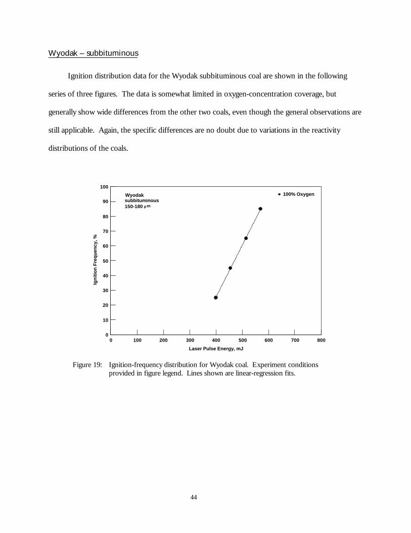
Wyodak – subbituminous
Ignition distribution data for the Wyodak subbituminous coal are shown in the following
series of three figures. The data is somewhat limited in oxygen-concentration coverage, but
generally show wide differences from the other two coals, even though the general observations are
still applicable. Again, the specific differences are no doubt due to variations in the reactivity
distributions of the coals.
100% Oxygen
mµµ150-180subbituminousWyodak
0 100 200 300 400 500 600 700
Laser Pulse Energy, mJ
8000
10
20
30
40
50
60
70
80
90
Ign
itio
n F
req
uen
cy, %
100
Figure 19: Ignition-frequency distribution for Wyodak coal. Experiment conditionsprovided in figure legend. Lines shown are linear-regression fits.

45
100% Oxygen50% Oxygen
Wyodaksubbituminous
mµµ106-125
0
10
20
30
40
50
60
70
80
90
Ign
itio
n F
req
uen
cy, %
100
0 100 200 300 400 500 600 700 800
Laser Pulse Energy, mJ
Figure 20: Ignition-frequency distribution for Wyodak coal. Experiment conditionsprovided in figure legend. Lines shown are linear-regression fits.
100% Oxygen50% Oxygen
Wyodaksubbituminous63-75 µµ m
0
10
20
30
40
50
60
70
80
90
100
Ign
itio
n F
req
uen
cy, %
0 100 200 300 400 500 600 700
Laser Pulse Energy, mJ
800
Figure 21: Ignition-frequency distribution for Wyodak coal. Experiment conditionsprovided in figure legend. Lines shown are linear-regression fits.

46
Illinois #6 – high-volatile C bituminous
Limited ignition-frequency data for the Illinois #6, high-volatile C bituminous coal is shown
in Figure 22. The behavior is dramatically different from the Pittsburgh high-volatile A bituminous
coal (see Figure 16) under similar experimental conditions. The differences include the slope of the
distribution at 100% oxygen concentration, as well as the shift to higher laser energy and slope
change when oxygen is decreased. The data shows that, even for coals of the same rank and similar
elemental make-up, ignition behavior can be quite varied.
100% Oxygen50% Oxygen106-125 µµ m
Illinois #6high-volatile C bituminous
0 100 200 300 400 500 600 700 800
Laser Pulse Energy, mJ
0
10
20
30
50
60
70
80
90
100
Ign
itio
n F
req
uen
cy, %
40
Figure 22: Ignition-frequency distribution for Illinois #6 coal. Experiment conditionsprovided in figure legend. Lines shown are linear-regression fits.
IV. Temperature Measurements
We have temperature measurements on a limited number of experiments, using one
particular coal of one size. The Pittsburgh #8 (DECS-23), high-volatile A bituminous coal of size
range 125-150 µm in diameter was chosen for this work. Our choice was dictated mainly by our

47
realization that (1) a large amount of sample was needed to diagnose and troubleshoot our
pyrometry system, (2) the coal must be of relatively large size for ease of signal detection (high
signal-to-noise ratio), (3) an extensive database of ignition frequency is available, and (4) the coal
must have a relatively high reactivity for this first set of measurements. This particular coal (herein
after referred to as the Base Coal) fits these criteria.
The ignition-frequency distribution of this coal is shown in Fig. 23. We have taken these data
on multiple days, and have confidence in their accuracy and precision with our experiment. The
data is consistent with those presented previously for this coal of both smaller and larger sizes.
Laser Pulse Energy, mJ
100 200 300 400 500 600 700 800
Igni
tion
Fre
quen
cy, %
0
20
40
60
80
100
Figure 23: Ignition-frequency distribution of Pittsburgh #8 (DECS-23) coal, 125-150 µmdiameter. Solid symbols are data taken at 100% oxygen concentration, andopen symbols are data for 50% oxygen concentration.
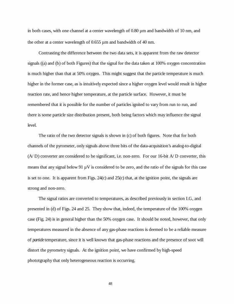
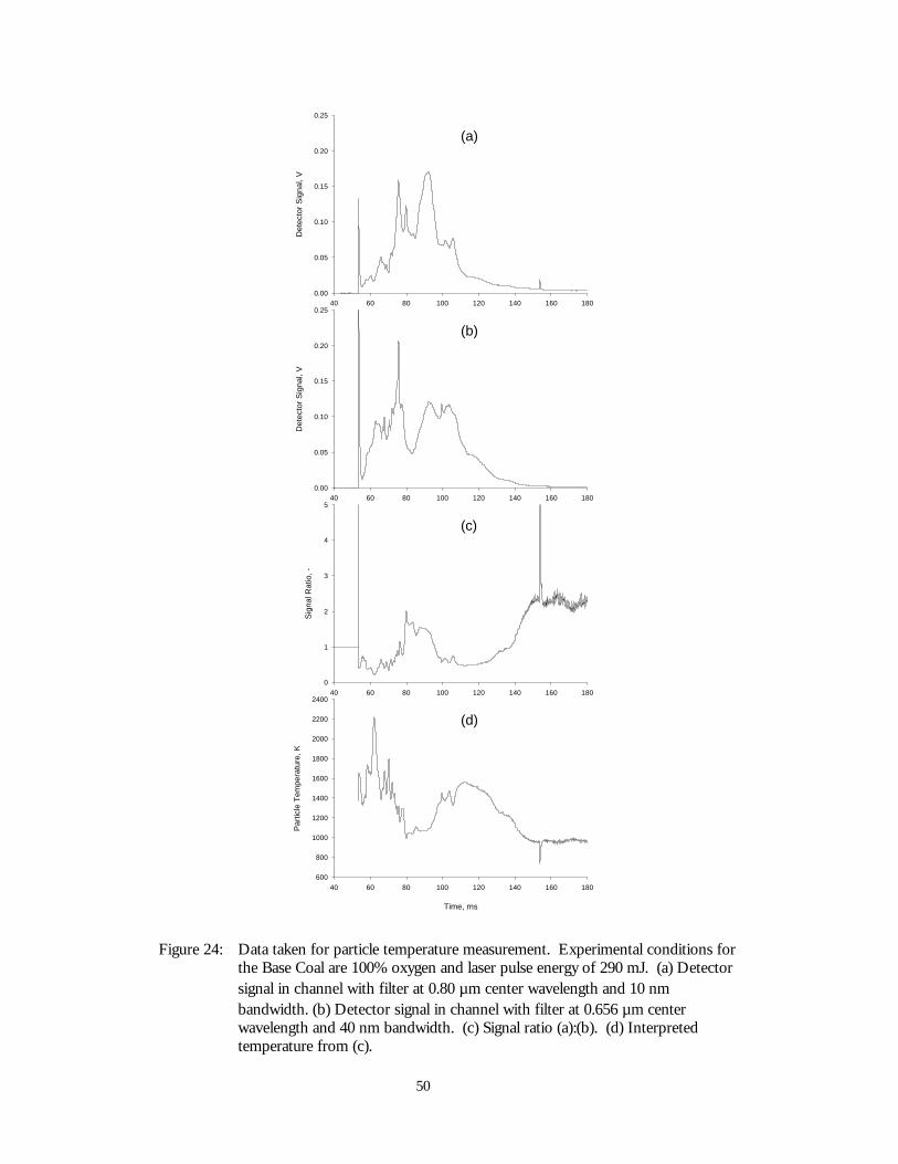
Figures 24 and 25 show data from ignition experiments of the Base Coal, both at a laser
energy equivalent to an ignition frequency of 50%. Figure 24 is taken at an oxygen concentration of
100%, while Fig. 25 is at 50% oxygen concentration. The same pyrometry system set-up was used
48
in both cases, with one channel at a center wavelength of 0.80 µm and bandwidth of 10 nm, and
the other at a center wavelength of 0.655 µm and bandwidth of 40 nm.
Contrasting the difference between the two data sets, it is apparent from the raw detector
signals ((a) and (b) of both Figures) that the signal for the data taken at 100% oxygen concentration
is much higher than that at 50% oxygen. This might suggest that the particle temperature is much
higher in the former case, as is intuitively expected since a higher oxygen level would result in higher
reaction rate, and hence higher temperature, at the particle surface. However, it must be
remembered that it is possible for the number of particles ignited to vary from run to run, and
there is some particle size distribution present, both being factors which may influence the signal
level.
The ratio of the two detector signals is shown in (c) of both figures. Note that for both
channels of the pyrometer, only signals above three bits of the data-acquisition’s analog-to-digital
(A/D) converter are considered to be significant, i.e. non-zero. For our 16-bit A/D converter, this
means that any signal below 91 µV is considered to be zero, and the ratio of the signals for this case
is set to one. It is apparent from Figs. 24(c) and 25(c) that, at the ignition point, the signals are
strong and non-zero.
The signal ratios are converted to temperatures, as described previously in section I.G, and
presented in (d) of Figs. 24 and 25. They show that, indeed, the temperature of the 100% oxygen
case (Fig. 24) is in general higher than the 50% oxygen case. It should be noted, however, that only
temperatures measured in the absence of any gas-phase reactions is deemed to be a reliable measure
of particle temperature, since it is well known that gas-phase reactions and the presence of soot will
distort the pyrometry signals. At the ignition point, we have confirmed by high-speed
phototgraphy that only heterogeneous reaction is occurring.

49
For the 100% oxygen case, the ignition temperature is found to be 1310 K, while for the 50%
case, the ignition temperature is found to be 1460 K. The ignition temperature is higher for the
latter case due to the higher laser energy required to reach 50% ignition frequency at the lower
oxygen level. We found a distribution in the ignition temperature measured at each experimental
condition; this is no doubt due to the variations in reactivity and perhaps size among the particle
sample. We learned from these first measurements that it will be essential to take data for a large
number of runs at each condition in order to build up meaningful statistics for data interpretation.
50
40 60 80 100 120 140 160 180D
etec
tor
Sig
nal,
V0.00
0.05
0.10
0.15
0.20
0.25
40 60 80 100 120 140 160 180
Det
ecto
r S
igna
l, V
0.00
0.05
0.10
0.15
0.20
0.25
40 60 80 100 120 140 160 180
Sig
nal R
atio
, -
0
1
2
3
4
5
Time, ms
40 60 80 100 120 140 160 180
Par
ticle
Tem
pera
ture
, K
600
800
1000
1200
1400
1600
1800
2000
2200
2400
(a)
(b)
(c)
(d)
Figure 24: Data taken for particle temperature measurement. Experimental conditions forthe Base Coal are 100% oxygen and laser pulse energy of 290 mJ. (a) Detectorsignal in channel with filter at 0.80 µm center wavelength and 10 nmbandwidth. (b) Detector signal in channel with filter at 0.656 µm centerwavelength and 40 nm bandwidth. (c) Signal ratio (a):(b). (d) Interpretedtemperature from (c).

51
50 75 100 125
Det
ecto
r S
igna
l, V
0.00
0.01
0.02
0.03
50 75 100 125
Det
ecto
r S
igna
l, V
0.00
0.01
0.02
0.03
50 75 100 125
Sig
nal R
atio
, -
0
1
2
3
4
5
Time, ms
50 75 100 125
Par
ticle
Tem
pera
ture
, K
600
800
1000
1200
1400
1600
1800
2000
2200
2400
2600
(a)
(b)
(c)
(d)
Figure 25: Data taken for particle temperature measurement. Experimental conditions forthe Base Coal are 50% oxygen and laser pulse energy of 730 mJ. Figuredescriptions are same as for Fig. 24.

52
V. Ignition-Rate Data
The interpretation of the temperature measurements shown in the previous section is made
difficult by the existence of ignition temperature variations from run to run, even under otherwise
identical experimental conditions. We currently have no means to deal with this finding to extract
rate constants from our data. The problem is further hampered by two factors: (1) We need to
make extensive measurements of ignition temperature at each condition in order to build up a large
database of ignition-temperature statistics, and (2) we need to develop a means to extend our data-
interpretation tool, the Distributed Activation Energy Model of Ignition, to handle our
experimental findings.
Currently, we can only extract the ignition rate constant for the Pittsburgh #8 coal by using
the limited ignition temperatures presented above in conjunction with simplifying assumptions
regarding the expected ignition behavior with oxygen and size variations. By assuming a reaction
order, n, of 1, and a preexponential factor of 500 kg/(m2s), we find the ignition rate constant
distribution to have an average activation energy of 73 kJ/mol, with a standard deviation, σ, of
3.7 kJ/mol.

53
Conclusions
We established a novel experiment to study the ignition of pulverized coals under conditions
relevant to utility boilers. Specifically, we determined the ignition mechanism of pulverized-coal
particles under various conditions of particle size, coal type, and freestream oxygen concentration.
We also measured the ignition rate constant of a Pittsburgh #8 high-volatile bituminous coal by
direct measurement of the particle temperature at ignition, and incorporating this measurement into
a mathematical model for the ignition process.
The ignition mechanism of pulverized coals in this experiment, under all conditions
examined, was determined by high-speed photography to be heterogeneous. That is, ignition of the
particles always occurred on the solid surface, prior to the evolution of volatile matter from the
particles into the gas phase. This finding was most likely due to the high heating rates achieved
(>105) by the laser heating, which causes the particle temperature to rise above that necessary for
ignition before appreciable devolatilization occurred.
Particle temperature at ignition was measured for one size group (125-150 µm) of one coal
(Pittsburgh #8, high-volatile bituminous) under two oxygen concentrations. At 100% oxygen, the
ignition temperature of this coal was found to be 1310 K, while at 50% oxygen the ignition
temperature was 1460 K. The higher temperature was expected since, for a lower oxygen level, a
higher temperature will be needed to cause particle ignition. Also, it was found that a distribution
of ignition temperature exists at each experimental condition. This is believed to be a result of the
particle-to-particle variations in reactivity and size among the coal sample.
The measured ignition temperatures were analyzed using the Distributed Activation Energy
Model of Ignition, and the ignition rate constant was determined to have an average value of 73
kJ/mol with a standard deviation of 3.7 kJ/mol. It is imperative to collect an extensive set of
ignition data in order to establish meaningful statistics for the extraction of ignition rate constants.

54
Impact on Infrastructure and Human Resources
This project has provided North Carolina A&T State University with enormous infrastructure
benefits, including over $60,000 worth of major equipment. Items gained as a direct result of this
project’s support includes a Nd:YAG laser system and associated optics, optical benches and tables,
various electronics, the wind tunnel used in this study, and a computer for data acquisition and
analysis.
Indirectly, this project attracted the support of the Department of Mechanical Engineering in
securing non-federal equipment funding. A digital oscilloscope, a digital pulse generator, and a PC-
based data-acquisition system – items purchased for over $19,000 – were acquired as a result.
In terms of human resources, this project supported three graduate students with salary and
tuition, and six undergraduate students with salary during its three-year span. The first graduate
student received his MS degree in the second year of this project [6], and another graduate student
will complete his degree requirements during the 1998-99 academic year.

55
Suggestions for Future Work
This project has demonstrated that particle temperature can be measured in our novel, laser-
based ignition experiment, and that the data can be interpreted using a unique model of coal
ignition. The model more realistically represents the ignition reactivity of the coals within a sample,
and permits the extraction of meaningful ignition rate constants from the measured temperatures.
The project period, being dominated by experiment development, did not permit enough coal types
to be examined, nor did it permit more careful optimization of the pyrometry system. Thus, the
major recommendations for future work are to:
1. refine the pyrometry system by improving the signal-to-noise ratio (e.g., by improving
light collection and transmission efficiency) to permit the use of more widely separated
filter wavelengths in order to improve temperature-measurement accuracy;
2. make additional measurements of ignition rate constants for a variety of coals and a range
of particle sizes and oxygen concentrations in order to establish a large database of
ignition temperatures for statistical analysis using the DAEMI;
3. develop a means to compare the rate constants from this experiment with previously
reported rate constants, which relied on different experimental techniques and methods
of data analyses.
Our final recommendation is for the extension of this project’s products – the ignition rate
constants and the Distributed Activation Energy Model of Ignition – into practical applications.
For example, these products may be incorporated into a model of the ignition of clouds of coal
particles, which would be of obvious benefit in the design of low-NOx burners and the prevention
of coal dust in mine shafts. Incorporation of the concepts and methods developed from this
project would more realistically model the fuel characteristics with regard to reactivity distribution,

56
and could possibly lead to new insights on flame propagation otherwise unobtainable using more
simplistic averaging to describe reactivity.

57
References
1 Essenhigh, R.H., Mahendra, K.M., and Shaw, D.W. Combust. Flame, 77:3-30 (1989).
2 Hurt, R.H. Energy Fuels, 7:721-733 (1993).
3 Chen, J.C. “Distributed Activation Energy Model of Heterogeneous Coal Ignition,” Combust.Flame, 107, 291 (1996).
4 Chen, J.C., Taniguchi, M., Narato, K., and Ito, K. Combust. Flame 97:107-117 (1994).
5 Zhang, D., Wall, T.F., Harris, D.J., Smith, I.W., Chen, J., and Stanmore, B.R. Fuel, 71:1239-1246 (1992).
6 Musti, Subrahmanyam S. Ignitability of Various Coals as Measured by Laser Ignition, MS thesis,Department of Chemical Engineering, North Carolina A&T State University (1996).

B-1
Appendices
A. Reprint of published paper: “Distributed Activation Energy Model of Heterogeneous
(NOTE: This document available only in the hardcopy version of this report.)


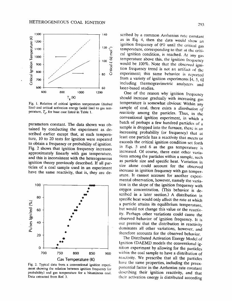


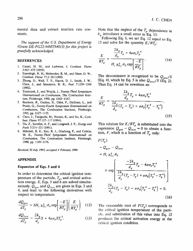
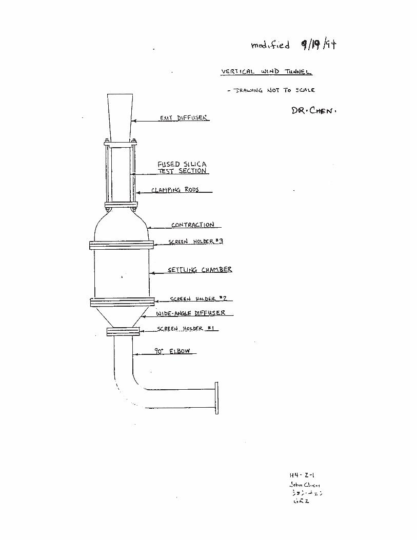

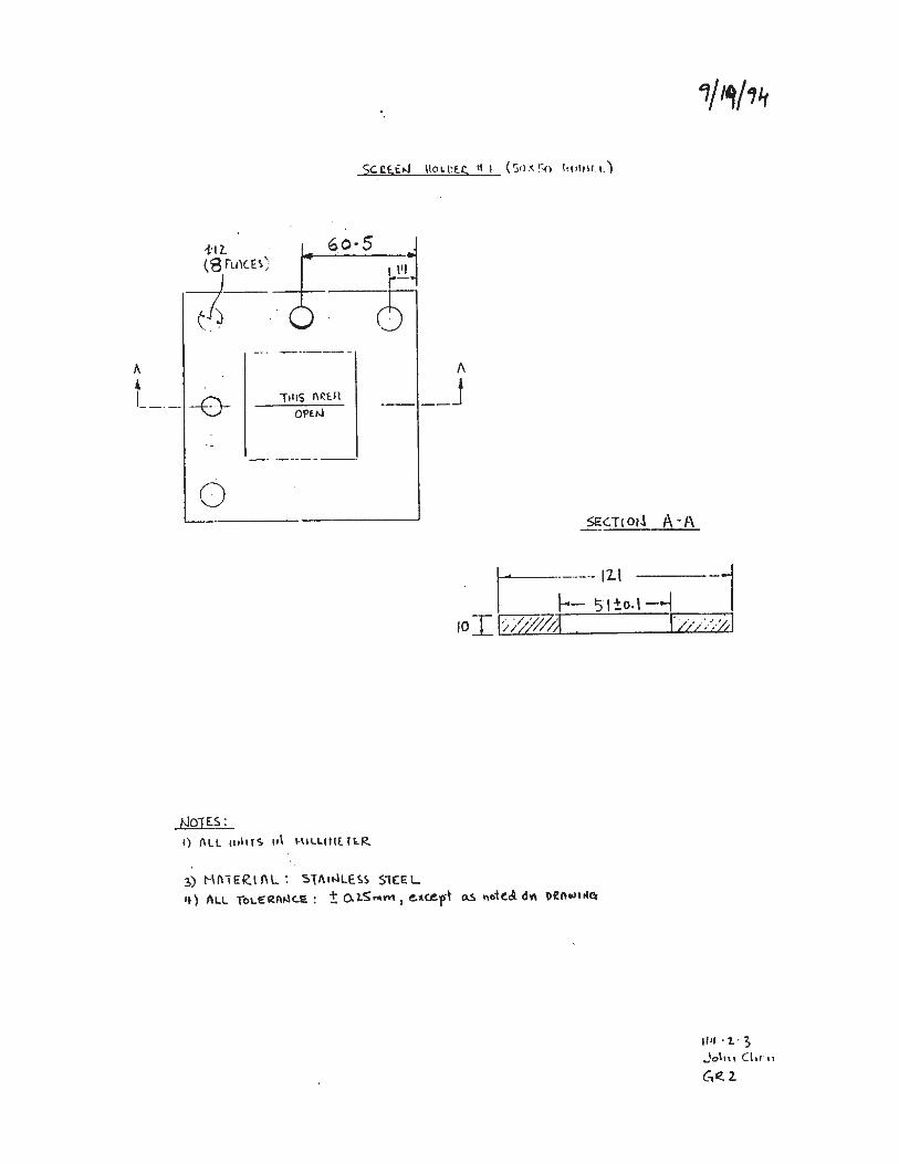

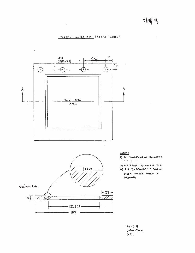
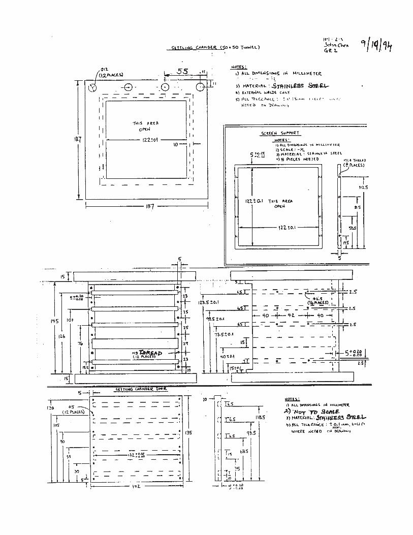


B-1
B. Engineering drawings of wind tunnel
(NOTE: These drawings are available only in the hardcopy version of this report.)

C-1
C. Detailed experimental procedure
1. Place coal in oven and create vacuum pressure of approximately 29 in Hg and heat to 72oC.
Leave coal in oven for 24 hours.
Next Day:
1. Remove coal from oven. Turn the oven off.
2. Follow start-up procedure (on wall).
3. Turn on the air to the automatic feeder and gate.
4. Turn on the two pulse generators and the oscilloscope. Set laser control to program 2. Turn
the bottom pulse generator to internal setting while simultaneously turning on the voltage
supply.
5. Check to see if the lenses are aligned. Then check to see if the prisms are aligned correctly using
the alignment rod. Make sure that the alignment rod is centered inside the quartz tunnel. If the
prisms are not aligned adjust them till you can see that both of the beams are vertical to one
another and intersect each other at the designated area of the alignment rod.
6. Turn on the gas flow of oxygen and nitrogen and set it to the selected flow rate and oxygen
concentration.
7. Take coal out of oven and allow it to cool. Place the appropriate mesh size into the feeder and
then pour the selected type coal on top of it.
8. Place and tighten the feeder inside the holder and line up the bottom of the holder to the blue
line on the pole. Align feeder tube so that it is centered inside the quartz tunnel.

C-2
9. Place a light behind the outlet of the feeder tube and trigger the automatic feeder without firing
the laser. Make sure that the back collar of the pneumatic trigger is what hits the feeder. This is
done to create consistency in the experiment. Measure the time it takes the coal to exit the
feeder and out of the feeder tube and reach the lasers height. View how far the coal particles
drop before the gas flow pushes it back up. The coal should drop approximately 2 cm and take
approximately 2.31 seconds.
10. Set the oscilloscope to record the ignition by pressing the run/stop button in the upper right
hand corner. When the oscilloscope is ready the ready output should show a green light. To run
experiment trigger the automatic feeder and gate by shifting the top pulse generator to external
pulse and quickly shifting it back to single shot. Record whether there was an ignition or just a
spark. Manually reset the feeder trigger.
11. Step 10 is repeated up to 19 times to complete a run.
12. After a run is completed clean the quarts tunnel. Tape a sheet of lens cleaning paper to the end
of the cleaning tube and wet the sheet of paper with alcohol. Also blow the excess particles of
coal out of the tunnel by turning of the oxygen and increasing the nitrogen flow rate.
After finishing experiment each day:
1. Cut off the power generator while simultaneously placing the bottom pulse generator on
internal pulse.
2. Cut off both pulse generators and the oscilloscope.
3. Shut down procedure (on wall).
4. Cut off Nitrogen and Oxygen

C-3
5. Turn off the air to the automatic trigger and automatic gate.
6. Cover all optics and prisms with specified plastic bags.
7. Clean wind tunnel and then cover the wind tunnel opening with a plastic bag.
8. Cover the whole table with the large plastic covering.
9. Throw out used coal.

D-1
D. Ignition-frequency data in tabular format
Table D-1: Experiment Data for Pittsburgh #8 (DECS 23) Coal.
Size (µm) 63-75 106-125 150-180
OxygenConcentration (%)
Elaser
(mJ)IgnitionFreq.
Elaser
(mJ)IgnitionFreq.
Elaser
(mJ)IgnitionFreq.
100 220255290340
2/206/2012/2018/20
170220280340
1/209/2011/2017/20
220280340400
5/209/2013/2016/20
75 255280340375
1/109/2015/2016/20
220280340455520
3/206/1010/2016/2010/10
280340455515
4/2010/2015/2018/20
50 280340400455
1/207/2014/2019/20
280340400455570
4/206/207/205/1018/20
455570655725
4/2010/209/2011/20
Table D-2: Experimental Data for Pittsburgh #8 DECS 23) Coal (second set).
Size (µm) 125-150Date: 7/30/97 8/7/97 & 8/13/97 9/3/97OxygenConcentration (%)
Elaser
(mJ)IgnitionFreq.
Elaser
(mJ)IgnitionFreq.
Elaser
(mJ)IgnitionFreq.
100 220240280302.5340
0/106/209/2015/2017/20
220240280302.5340
3/2011/2016/2014/2010/10
220280302.5340
7/209/1014/2010/10
50 455570615655755
4/208/205/209/2011/20
340455570
5/2012/2014/20
340455570
0/203/2011/20

D-2
Table D-3: Experimental Data for Wyodak (DECS 26) Coal.
Size (µm) 63-75 106-125 150-180OxygenConcentration (%)
Elaser
(mJ)IgnitionFreq.
Elaser
(mJ)IgnitionFreq.
Elaser
(mJ)IgnitionFreq.
100 125170220280340
0/103/207/208/2016/20
170220340455570
1/107/2010/209/1010/10
400455515570
5/209/2013/2017/20
50 340455570655725742
3/205/208/2012/2016/2016/20
460655725
0/203/204/20
Table D-4: Experimental Data for Sewell (DECS 13) Coal.
Size (µm) 106 -125OxygenConcentration (%)
Elaser
(mJ)IgnitionFreq.
100 220255280340
2/208/2013/2016/20
75 220280340400455
2/206/209/2011/2016/20
50 455520620655700725
4/206/206/209/2010/2013/20

D-3
Table D-5: Experimental Data for Illinois #6 (DECS 24) Coal.
Size (µm) 106-125OxygenConcentration (%)
Elaser
(mJ)IgnitionFreq.
100 220340460520570
3/208/2014/2015/2010/10
50 655725755
0/203/206/20