Project no. TREN/07/FP6AE/S07.71574/037180 IFLY

iFly

Safety, Complexity and Responsibility based design and validation of highly automated Air Traffic Management

Specific Targeted Research Projects (STREP) Thematic Priority 1.3.1.4.g Aeronautics and Space

iFly Deliverable D3.1 Complexity metrics applicable to autonomous aircraft

Version: Final (1.1)

Authors: M. Prandini (PoliMi), L. Piroddi (PoliMi), S. Puechmorel (ENAC), S.L. Brázdilová (HNWL)

Due date of deliverable: 22 February 2008 Actual submission date: 14 January 2009

Start date of project: 22 May 2007 Duration: 39 months

Project co-funded by the European Commission within the Sixth Framework Programme (2002-2006) Dissemination Level

PU Public X PP Restricted to other programme participants (including the Commission Services) RE Restricted to a group specified by the consortium (including the Commission Services) CO Confidential, only for members of the consortium (including the Commission Services)

iFly 6th Framework programme Deliverable D3.1

14 January, 2009 TREN/07/FP6AE/S07.71574/037180 IFLY

DOCUMENT CONTROL SHEET

Title of document: Complexity metrics applicable to autonomous aircraft Authors of document: Maria Prandini, Luigi Piroddi, Stehane Puechmorel, Silvie Luisa Brázdilová

Deliverable number: D3.1 Project acronym: iFly

Project title: Safety, Complexity and Responsibility based design and validation of highly automated Air Traffic Management

Project no.: TREN/07/FP6AE/S07.71574/037180 IFLY Instrument: Specific Targeted Research Projects (STREP)

Thematic Priority: 1.3.1.4.g Aeronautics and Space

DOCUMENT CHANGE LOG Version # Issue Date Sections affected Relevant information

0.1 20.02.2008 all First Draft 0.2 26.03.2008 all Second Draft 0.3 01.04.2008 Chapters 4 and 5 Third Draft (added chapter 4) 1.0 19.06.2008 all Final 1.1 14.01.2009 Chapter 1 Change in iFly

Version 1.1 Organisation Signature/Date Authors Maria Prandini PoliMi

Luigi Piroddi PoliMi Stephane Puechmorel ENAC Silvie Luisa Brázdilová HNWL

Internal reviewers Henk Blom NLR

External reviewers Prof. Dr. Uwe Voelckers EC

iFly, Work Package 3, D3.1

Complexity metrics applicable to autonomous aircraft

14 January, 2009

Abstract

This is the first deliverable of work package 3 of the iFly project. Theobjective of work package 3 is to study and develop methods for timely pre-dicting potentially complex air traffic conditions that may be over-demandingto the autonomous aircraft design. The characterization of encounter situa-tions that appear safe from the individual aircraft perspective, but are actuallysafety-critical from a global perspective can provide useful information for thetrajectory management and conflict resolution operations, and can also help inidentifying the potential ground support needs within the autonomous aircraftAir Traffic Management (ATM) concept developed in the iFly project.

Deliverable 3.1 consists in a comparative study of the different metrics pro-posed in the literature for complexity characterization and prediction in ATM.Most of the metrics address ground-based ATM and are conceived so as to as-sess the impact of a given air traffic configuration on the workload of the airtraffic controllers in charge of safely handling it. We review these metrics inview of a possible application to advanced autonomous aircraft ATM systems.

1

Contents

1 Introduction 4

1.1 iFly work package 3 . . . . . . . . . . . . . . . . . . . . . . . . . . . 4

1.2 Objectives of Deliverable 3.1 . . . . . . . . . . . . . . . . . . . . . . 5

1.3 Organization of the document . . . . . . . . . . . . . . . . . . . . . . 5

2 Air traffic complexity studies in the literature 7

2.1 Introduction . . . . . . . . . . . . . . . . . . . . . . . . . . . . . . . . 7

2.2 Approaches to air traffic complexity modelling and prediction withinground-based ATM . . . . . . . . . . . . . . . . . . . . . . . . . . . . 10

2.2.1 Aircraft density . . . . . . . . . . . . . . . . . . . . . . . . . . 10

2.2.2 Dynamic density . . . . . . . . . . . . . . . . . . . . . . . . . 11

2.2.3 Interval complexity . . . . . . . . . . . . . . . . . . . . . . . . 15

2.2.4 Fractal dimension . . . . . . . . . . . . . . . . . . . . . . . . 15

2.2.5 Input-output model . . . . . . . . . . . . . . . . . . . . . . . 16

2.2.6 Intrinsic complexity measures . . . . . . . . . . . . . . . . . . 17

2.3 Discussion on the approaches to air traffic complexity . . . . . . . . 18

2.3.1 The workload issue . . . . . . . . . . . . . . . . . . . . . . . . 18

2.3.2 Classification of the revised approaches . . . . . . . . . . . . 21

2.4 Concepts related to air traffic complexity . . . . . . . . . . . . . . . 25

2.4.1 Trajectory flexibility . . . . . . . . . . . . . . . . . . . . . . . 25

2.4.2 Aircraft clustering . . . . . . . . . . . . . . . . . . . . . . . . 25

3 A dynamical approach to intrinsic air traffic complexity character-ization 29

3.1 The underlying principle . . . . . . . . . . . . . . . . . . . . . . . . . 29

3.2 Lyapunov exponents as complexity indicator . . . . . . . . . . . . . . 30

3.2.1 Definition and properties . . . . . . . . . . . . . . . . . . . . 30

3.2.2 Computational aspects . . . . . . . . . . . . . . . . . . . . . . 36

3.3 Modelling air traffic as a dynamical system . . . . . . . . . . . . . . 38

4 Conclusions and future work 40

2

List of Figures

1 Managed airspace control scheme. . . . . . . . . . . . . . . . . . . . 7

2 Mid-term enroute control in ground-based ATM. . . . . . . . . . . . 8

3 Mediating factors affecting the impact of air traffic complexity onworkload. . . . . . . . . . . . . . . . . . . . . . . . . . . . . . . . . . 19

4 Model of the Air Traffic Controller, [37]. . . . . . . . . . . . . . . . . 19

5 Complexity evaluation within ground-based ATM. . . . . . . . . . . 20

6 Control scheme in autonomous aircraft ATM. . . . . . . . . . . . . . 22

3

1 Introduction

An Air Traffic Management (ATM) system is a multi-agent system, where manyaircraft are competing for a common, congestible resource, represented by airspaceand runways space, while trying to optimize their own cost (travel distance, fuelconsumption, passenger comfort, etc.). Coordination between different aircraft isneeded to avoid conflicts where two or more aircraft get too close one to the other.In principle, this can be achieved via a decentralized control scheme where eachaircraft evaluates the criticality of forthcoming encounters based on the informa-tion on the current position and intended destination of neighboring aircraft, andeventually coordinates with them to avoid that a conflict actually occurs. Noticethat in a decentralized approach to conflict detection each aircraft employs localinformation only, and evaluates the criticality of the situation based on a partialviewpoint. A high-level coordination layer can possibly be required to avoid safety-critical encounters corresponding to a level of risk that is considered low by theaircraft involved, but is actually high for the overall multi-aircraft system.

1.1 iFly work package 3

The objective of work package 3 is to study and develop methods for the timelyprediction of air traffic conditions that may be over-demanding to the autonomousaircraft design. This is a crucial task for avoiding encounters that appear safe fromthe individual aircraft perspective, but are actually safety-critical from a globalperspective. The characterization of globally safety-critical encounters can provideuseful information for the trajectory management and conflict resolution operations,and can also help in identifying the potential ground support needs within theautonomous aircraft ATM concept developed in work package 1 of the iFly project.

Work package 3 is structured in the following two sub-work packages:

WP3.1: Comparative study of complexity metrics. In this sub-work pack-age, we shall carry out a critical survey of different metrics proposed in theliterature for complexity modelling and prediction in ATM. Most of the cur-rent complexity metrics address ground-based ATM. Though this is reason-able within the current centralized ATM system, where aircraft follow prede-fined routes according to some prescribed 4D flight plan, it becomes restrictivewithin advanced autonomous aircraft ATM systems.

WP3.2: Timely predicting complex conditions. In this sub-work package, weshall study the problem of predicting complex conditions for autonomous air-craft and developing an appropriate complexity metric. Aspects that needto be addressed are the sensitivity to the prediction time, and various otherconditions. For work package 3 studies no specific choice is made regarding

4

where to use the novel method, airborne and/or on the ground.

Work package 3 will receive input from work package 1, in terms of the AutonomousAircraft Advanced Concept of Operations (A3 ConOps). WP3 will provide input towork package 8 as for ground support needs for the A3 ConOps, thus contributingto the refinement of the A3 ConOps. Appropriate interaction with work packages1 and 8 is required to identify potential areas of usage of complexity metrics andclarify the requirements for the developed metrics.

The specification of the requirements on complexity metrics for the A3 ConOps isone of the first activities planned under WP3.2, based on the precise formalizationof the A3 ConOps in Deliverable 1.3. As for the output to work package 8, a phase oftuning with WP8.1 is planned for the last stage of WP3.2. The objective of WP8.1is in fact integrating within the A3 ConOps the innovative methods for complexityprediction and for multi-agent situation awareness inconsistency identification andconflict resolution, developed within WP3, WP4, and WP5, respectively.

1.2 Objectives of Deliverable 3.1

Deliverable 3.1 is the outcome of the sub-work package 3.1 and consists in a com-parative study of the different approaches proposed in the literature for air trafficcomplexity modelling and prediction. Most of the current air traffic complexity stud-ies relates to ground-based ATM, where the airspace is divided into sectors and AirTraffic Controllers (ATCs) are in charge of guaranteeing safety in air travel withintheir sector. In Deliverable 3.1, we revise these studies in view of a possible applica-tion to advanced autonomous aircraft ATM systems, where part of the responsibilityin maintaining the appropriate separation between aircraft is delegated to the pilots.In particular, pilots will take over the ATC tasks for separation assurance in self-separation enroute airspace, and they will rely for this purpose on advanced toolsenabled by advanced technologies for sensing, communicating, and decision making.Centralized control will assume a new role consisting in a higher level, possibly au-tomated, supervisory function as opposed to lower level human-based control, whichshould allow an increase in the airspace capacity without compromising safety.Complexity measures that have been to some extent successful within the currenthuman-based centralized ATM system may actually be inappropriate within theforeseen automated self-separation airspace.

1.3 Organization of the document

Deliverable 3.1 is structured as follows. In Chapter 2 we illustrate the notion of airtraffic complexity within the current ground-based ATM. As pointed out in Section2.1, studying air traffic complexity is fundamental in this context to evaluate the im-pact on the ATC workload of possible modifications of the ATM system introduced

5

to adapt its capacity to the increased air traffic demand. For this reason, most ofthe measures of complexity proposed in the literature try to incorporate the diffi-culty perceived by ATCs in handling different air traffic situations. In order to use acomplexity metric as a traffic management tool, it is necessary to predict its futurebehavior. In Section 2.2 we describe some of the approaches for air traffic complexitymodelling and prediction, and in Section 2.3 we compare them in view of a possibleapplication to advanced autonomous aircraft ATM design. The complexity-relatedconcepts of trajectory flexibility and aircraft clustering are described in Section 2.4.In Chapter 3, we focus on an approach developed by ENAC that provides a measureof the intrinsic complexity of air traffic, independent of the ATCs perceived diffi-culty in accomplishing their task, and looks promising for application to advancedautonomous aircraft ATM. Finally, in Chapter 4 we draw some final conclusions onthis survey on air traffic complexity, outlining possible directions of research underWP3.2 on complexity characterization for enroute autonomous aircraft ATM.

6

2 Air traffic complexity studies in the literature

2.1 Introduction

The growth in air traffic demand is pushing to its limit the current ground-basedATM system. As reported in [28], in 2006 the average daily traffic above Europewas 26286 flights per day, with an increase of 4.1% over 2005, whereas the totaldelay increased by 4.6%, much more than expected based on the 4.1% of air trafficgrowth.

In Figure 1 managed airspace is represented as a control system where ATM acts asfeedback controller of the airspace. The thick lines connecting the ATM and airspaceblocks represent multi-dimensional signals (airspace measurements and ATM ac-tions). The objective of the ATM controller is to guarantee safety and efficiencyin air travel, despite the airspace system time-variability due, for instance, to tem-porary structural modifications when the access to some areas is forbidden becauseof military missions or bad weather conditions, and to disturbances like aircraftentering/leaving the airspace because departing/landing at airports.

Figure 1: Managed airspace control scheme.

The main components of the current ATM system are the Air Traffic Control andTraffic Flow Management functions. The former is in charge for maintaining theappropriate separation between aircraft within the airspace, whereas the latter hasto define the flow patterns so as to ensure a smooth and efficient organization ofthe air traffic. These two functions operate on different time scales, namely on amid-term and on a long-term time horizon, as detailed in Deliverable 5.1 of theiFly project entitled “Comparative Study of Conflict Resolution Methods” whereresolution methods are distinguished based the reference time-horizon. The airspaceis structured into Air Traffic Control Centers (ATCCs) partitioned into sectors, eachcontrolled by a team of 1 to 3 Air Traffic Controllers (ATCs). Sectors are designedso that the nominal flow of traffic through each sector can be safely handled by theATCs that are in charge of that sector. The ATCC capacity is limited by the sectorwith the minimum capacity.

The basic control unit in mid-term control is plotted in Figure 2. In the feedbackcontrol scheme, the controlled system is not the whole airspace but only a sector,and the feedback controller is represented by the ATC which interacts with the

7

controlled system through sensing and actuating interfaces. The exogenous input tothe control system represents aircraft entering/exiting the sector under considerationand models the interactions with neighboring sectors. Information on the controlledsystem behavior and on the exogenous input are provided to the ATC through“sensors” (radar, software equipment, and radio connections), whereas the controlstrategy is implemented issuing commands (speed, altitude, heading changes) to thepilots via radio connections (the “actuators”).

Figure 2: Mid-term enroute control in ground-based ATM.

A method to accommodate air traffic growth within the current ATM system isto adapt its capacity to the increased demand by appropriately redesigning theairspace, reconfiguring sectors, modifying traffic patterns, and also reassigning staff,[41, 83]. The most common operational means of increasing capacity is to parti-tion a sector into smaller ones, each with an independent controller team. Thesemodifications are currently adopted temporarily in presence of extraordinary events,as particular weather conditions or constraints on the airspace usage due, e.g., tomilitary missions. The purpose of such permanent or temporary modifications isto avoid an increase of the ATC workload, which could eventually compromise airtravel safety and efficiency.

Generally speaking, ATC workload can be regarded as the mental and physicaleffort involved in handling air traffic. In [66], workload is defined as “... a functionof three elements, firstly, the geometrical nature of the air traffic; secondly, theoperational procedures and practices used to handle the traffic and thirdly, thecharacteristics and behavior of individual controllers (experience, orderliness, etc.)...”. The configuration of sectors, in particular, is recognized as a main factoraffecting workload, [31], and workload is held responsible for limiting sector capacity[15, 59, 67, 61]. In [30, 85], a macroscopic workload model is studied to assess sectorcapacity.

Air traffic complexity, intended as a “... measure of the difficulty that a particulartraffic situation will present to an air traffic controller ...”, [66], is commonly thoughtas responsible for generating workload.

8

Since about forty years ago, air traffic complexity models have been studied to relateairspace configuration and traffic to the workload of ATCs, introducing indicatorsof the workload level that are based on airspace and air traffic measurements. Thework [18] is perhaps the first one to systematically examine the relationship betweenair traffic complexity and controller workload.

It is generally recognized that a measure of the difficulty experienced by ATCsin controlling air traffic is fundamental to evaluate how the current ground-basedATM system is operated, and that it could also provide guidelines on how to obtainmore manageable sectors by reconfiguring the airspace and by modifying trafficpatterns. In [29], it is suggested that the capacity of an ATCC could be increased bya timely prediction of the traffic complexity bottleneck areas and a reconfigurationof the traffic patterns so as to evenly balance traffic complexity between sectors.A “complexity resolution” algorithm is introduced for dynamically modifying flightprofiles to reduce the predicted complexity of more critical sectors and balancethe complexity of adjacent sectors. In [86], a methodology for optimal design ofairspace sectors is proposed. The airspace is partitioned into hexagonal cells andeach cell is assigned a workload measure. Then, the airspace sectors are constructedby clustering algorithms using optimization methods. In [65], indicators of sectorworkload are studied, that could be operationally useful to Traffic ManagementCoordinators (TMCs) taking decisions affecting how much traffic ATCs will have tohandle as well as traffic complexity.

In the current practice, complexity of air traffic is commonly evaluated in terms ofnumber of aircraft and on a per-sector basis, [83]. Many researchers have found thatair traffic indicators other than the number of aircraft are relevant to ATC workload.For instance, depending on the air traffic structure, ATC perceives situations withthe same number of aircraft in the sector as different. A list of “complexity factors”is provided in the literature review [37]. Most researchers agree that complexitydepends on both structural and flow characteristics of air traffic, [67, 37]. The formerare fixed for a sector and given by spatial and physical attributes such as terrainconfiguration, number of airways, airway crossings and navigation aids (static airtraffic characteristics). The latter vary as a function of time and depend on featuressuch as number of aircraft, weather, aircraft separation, closing rates, aircraft speeds,mix of aircraft and flow restrictions (dynamic air traffic characteristics). Thesestatic and dynamic factors interact in a nonlinear complex way to produce air trafficcomplexity, [4, 59, 13]. Nevertheless, according to the literature review [37], mostof the complexity metrics developed to date depend heavily on the traffic densityalone.

Besides planning and redesign, improved measures of complexity could be of usefor the evaluation of air traffic management productivity, and the assessment of theimpact of new tools and procedures, [37].

It is perhaps worth mentioning that air traffic complexity has been studied in rela-

9

tion not only with controller workload, but also with such different issues as:

- the occurrence of operational errors (events where two or more aircraft vio-late the separation standard and the cause is attribute to ATC) or incidents,[67, 36, 11, 76, 77, 84, 70];

- controller decision making, [68];

- the design of decision support and flight planning tools [19, 64, 78];

- conflict risk [3, 48, 80].

2.2 Approaches to air traffic complexity modelling and prediction

within ground-based ATM

Most studies on air traffic complexity in the literature have been developed withreference to ground-based ATM. In this section, we review selected approaches toair traffic complexity. For a more extensive overview, we suggest the comprehensiveliterature reviews [67, 37].

Strengths and weaknesses of each approach are presented within its description.A classification of the approaches based on characteristics that are relevant to au-tonomous aircraft ATM is postponed to Section 2.3.

2.2.1 Aircraft density

The number of aircraft in a sector is the air traffic characteristic that has been mostcited, studied, and evaluated in terms of its influence on workload. It is, at the sametime, considered as the best available indicator of complexity and criticized for notbeing able to appropriately characterize what controllers find complex. Currently,it is the complexity measure most adopted in practice, possibly because it is easierto interpret than other complexity measures: if the aircraft number exceeds theoperationally-defined threshold by four aircraft, then the situation is classified to beof high-workload, and it can be resolved by removing four aircraft.

Sectors are designed so that the controllers are able to handle the usual flow of traffic.In the event of increased demand or re-routing required due to weather conditions orspecial use airspace constraints, Traffic Flow Management (TFM) techniques suchas staff reallocation and alternative airspace configurations are used for maintainingthe ATCs workload constant so as not to compromise safety and efficiency levels. Inthe United States, the peak aircraft count (the largest number of aircraft in a sectorduring any minute of a 15 minutes time interval) is compared with an acceptablepeak traffic count value determined by traffic flow managers based on practicalexperience, and adopted for operational TFM decisions like re-routing flights out ofan overloaded sector, [65]. The drawbacks of this measure are that it is insensitiveto the duration of a high workload period, it is very sensitive to the entry and exit

10

times of a few flights which do not change the amount of sustained workload. Inaddition, this measure does not take into account such factors as the traffic pattern,traffic mix, weather, etc., that may greatly influence the actual workload levelsexperienced in practice. Finally, it is important to remark that operational errorsare more likely to occur after rather than during a peak in traffic count, as suggestedin [76], a simulation study involving a human-in-the-loop.

The European Flow Management Positions (FMP) staff determines the airspaceconfiguration schedule (successive aircraft configuration during the day) by splittingor merging sectors based on the number of ATCs on duty and the traffic load assessedby means of flight counts and sector capacities. In [32], it is suggested that morerealistic airspace configurations could be obtained by adopting more appropriatecomplexity metrics.

The Enhanced Traffic Management System (ETMS) is a decision support systemfor traffic management whose monitor/alert function is based on a comparison ofthe prediction of traffic volume in the sector against some established thresholdvolume representing the maximum number of aircraft that the ATCs are willing toaccept in that sector. Threshold volume, however, does not adequately representthe actual ATC workload since, in certain circumstances, controllers accept trafficbeyond the threshold, whereas, in other circumstances, they reject it although thenumber of aircraft is well below the threshold. The level of organization of thetraffic should be considered jointly with the air traffic volume, since, depending onthe air traffic structure, ATC perceives situations with the same number of aircraftin the sector as different. It is recognized by the Radio Technical Commission onAeronautics (RTCA) that this monitor/alert function should be integrated withmore precise measures of sector complexity and controller workload to adequatelyrepresent the level of difficulty experienced by the controllers under different trafficconditions, [1]. Also, the behavior in time of the traffic volume affects workload: atraffic volume that highly fluctuates over time is more likely to generate conflictsand appears more complex to the controller than a uniform traffic flow, [27]. Airtraffic controllers adapt their strategy to regulate the workload as the traffic vol-ume increases, sacrificing secondary objectives in order to maintain their principalobjectives, [81, 82]. For example, in a low traffic situation, they take into accountperformance objectives when solving conflicts, whereas, as the traffic level increased,they are only concerned with guaranteeing the appropriate separation between air-craft. Moreover, controllers select operating procedures based on economy, i.e., asair traffic density increases, they use less costly procedures to avoid overload.

2.2.2 Dynamic density

Dynamic density, [46, 56, 83, 49, 50, 64, 65], is a metric for assessing the controlleractivity level in a sector that was introduced within a research program in U.S.

11

involving FAA, NASA, MITRE, and Wyndemere Corporation as main participants.Laudeman et al from NASA, [56] defined dynamic density as “a measure of control-related workload that is a function of the number of aircraft and the complexity oftraffic patterns in a volume of airspace”.

Dynamic density is a single aggregate indicator obtained as a linear combinationof traffic density and other controller workload contributors (the number of air-craft undergoing trajectory change and requiring close monitoring due to reducedseparation) identified through interviews to several qualified air traffic controllers.

More precisely, dynamic density is the weighted sum of the number of aircraft andthe following aggregate indicators of the aircraft changing geometries during a one-minute sample time interval:

• the number of aircraft with heading change > 15 degrees,

• the number of aircraft with speed change > 0.02 Mach,

• the number of aircraft with altitude change > 750 ft,

• the number of aircraft with 3-D Euclidean distance between 0-5 nautical milesexcluding violations,

• the number of aircraft with 3-D Euclidean distance between 5-10 nautical milesexcluding violations,

• the number of aircraft with lateral distance between 0-25 nautical miles andvertical separation < 2000/1000 feet above/below 29000 ft,

• the number of aircraft with lateral distance between 25-40 nautical miles andvertical separation < 2000/1000 feet above/below 29000 ft,

• the number of aircraft with lateral distance between 40-70 nautical miles andvertical separation < 2000/1000 feet above/below 29000 ft.

The weights were determined both by subjective ratings obtained showing differenttraffic scenarios to the interviewed controllers and by regression analysis of con-trollers activity data. The dynamic density measure with subjective weights wasvalidated in an operational environment and showed to be highly correlated withobserved controllers activity, more than the traffic volume.

Note that the complexity indicators entering the dynamic density metric dependon the aircraft trajectories during a one-minute sample time interval and do notinclude observed metrics of the ATCs physical work such as data entry and radiocommunications. By using trajectory prediction tools, it is then possible to projectthe dynamic density measure over a suitable time horizon so as to forecast futureworkload levels and use this information for traffic management purposes.

12

In [83], the future values of the dynamic density in a sector are computed basedon the aircraft positions and speeds predicted by the Center-TRACON AutomationSystem (CTAS, [26]) using aircraft dynamic models, flight plans, radar tracks withinthe Air Route Traffic Control Center (ARTCC), and weather data.

Apparently, dynamic density can be accurately predicted 5 minutes in advance(short-term prediction). The long-term prediction over a 20 minutes time hori-zon is affected by errors that can be reduced by integrating in CTAS inter-Centerdata on aircraft entering the ARTCC. The performance obtained in the 20 minuterange prediction suggests that there is further room for improvement, both in thetrajectory prediction tool and in the dynamic structure of the model. Sources ofprediction errors are aircraft departures within the considered sector, wind predic-tion and radar tracker. Also, prediction does not take into account the ATCs action(open loop prediction).

There are some important weaknesses regarding dynamic density to be aware of.First of all, the computed weights are extremely variable from sector to sector andtherefore need to be re-estimated and re-validated for each sector (and possiblyperiodically retuned). Also, the proposed dynamic density model for air trafficcomplexity is actually a static model, that does not incorporate explicitly neitherfuture predicted aircraft topology, neither past state information. The predictionsof the dynamic density future behavior is calculated with the same equation usingthe predicted values of the complexity factors involved as provided by the adoptedtrajectory prediction tool. Therefore, the prediction capabilities allegedly attributedto the dynamic density indicator are in fact a merit of the prediction tool. Further-more, it is difficult for decision makers as Traffic Management Coordinators (TMCs)to understand from a single aggregate measure how to solve a high-workload sit-uation. Information on which complexity factor has caused the problem is in factlost. On the other hand, having too many complexity factors to analyze may slowdown the decision process due to overload in information processing. Potentiallynonlinear relations between complexity indicators are missed, [38]. The results ofthe dynamic density work could be improved by adopting non-linear techniques, in-cluding neural networks, genetic algorithms, and non-linear regression, [50]. Finally,the adopted indicator of the controller workload used to determine the weights iscritical. Behavioral measurements miss the cognitive aspects of controller activity.Subjective ratings are often subject to biases.

Dynamic density is used in a variety of contexts in the literature and does notcorrespond to a single metric. Overall, there is a significant consensus over 20-30dynamic density metrics. Most of the factors used in dynamic density models aredynamic traffic characteristics that are generally useful for realtime decision support.Various linear and nonlinear methods are used to perform the correlation.

A human-in-the-loop simulation study with controllers actively controlling traffic ina real-time simulation environment was performed in [52] with the two-fold objective

13

of introducing a new dynamic density complexity model and of validating dynamicdensity versus aircraft count. In [51], it was also shown that the measurement ofcomplexity using the dynamic density is better than a simple aircraft count for boththe instantaneous and the predicted complexity measures.

In [65], the use of dynamic density as an operationally useful sector workload mea-sure for enabling TFM personnel to prevent overloads is investigated. The dynamicdensity metric is defined as the weighted sum of multiple sector workload factors. 12complexity factors out of a set of 41 were selected based on their correlation to thesubjective measure of the workload experienced by ATCs and their predictability,avoiding redundancy. The study of the dependence of the resulting dynamic densitymetric on the considered airspace reveals that different factors contribute to theperceived difficulty in different centers.

The instantaneous positions and speeds of the traffic itself do not appear to beenough to describe the total complexity associated with an airspace. Efforts to de-fine dynamic density have identified the importance of a wide range of potentialcomplexity factors, including structural considerations. A few previous studies haveattempted to include structural consideration in complexity metrics, but have doneso only to a restricted degree. The importance of including structural considera-tion has been explicitly identified in work at Eurocontrol. In a study to identifycomplexity factors using judgement analysis, Airspace Design was identified as thesecond most important factor behind traffic volume [54]. Histon et al. [39, 40]investigated how this structure can be used to support structure-based abstrac-tions that controllers appear to use to simplify traffic situations (cognitive aspectaffecting workload). Within the dynamic density research program, the WyndemereCorporation proposed a dynamic density metric that included a term based on therelationship between aircraft headings and the dominant geometric axis in a sector[46]. Also, specific emphasis on the traffic and airspace characteristics that impactthe cognitive and physical demands placed on the controller was given. An attemptwas made to include the level of knowledge about the intent of the aircraft.

Many approaches to air traffic complexity characterization by a dynamic densitymodel similar to that in [56] are proposed in the literature (see, e.g., the survey [37]),where various sector and aircraft status indicators are correlated to the perceivedworkload on a relevant dataset of ATC activity recording. In [39], sector workloadfactors to be combined in a single workload metric are classified into airspace de-sign factors, dynamic traffic characteristics, and operational factors, and a list percategory is provided. The importance of representing complexity in a way that canhelp TMCs deciding on actions affecting the ATCs workload is pointed out in [65].

14

2.2.3 Interval complexity

Recently, the interval complexity of a sector was introduced as an estimate of theATC workload in that sector, [29]. The interval complexity of a sector is defined asthe average over a time window of the linear combination of the following complex-ity factors: number of aircraft flying within the sector, number of aircraft flying onnonlevel segments, and number of aircraft flying close to the border. Nonlevel flightsand flights close to the boundary of a sector in fact require special attention andprocedures to be followed by the ATC. The weights in the linear combination dependon the specific sector. Interval complexity can be considered as a smoothed versionof a dynamic density-like complexity measure. The prediction of this measure ofcomplexity over a time horizon of 20 to 90 minutes is used for selecting appropri-ate “complexity resolution” actions minimizing and balancing traffic complexitiesbetween adjacent sectors of a certain airspace region.

2.2.4 Fractal dimension

A characterization of traffic structure based on the fractal dimension of the trafficpattern has been proposed in [69]. Fractal dimension is a metric suggested for com-paring traffic configurations resulting from various operational concepts. It allowsin particular to decouple the complexity due to airspace partitioning in sectors fromthe complexity due to traffic flow features.The dimension of (compact) geometrical figures is well-known: a curve is of dimen-sion 1, a surface of dimension 2, and so on. It is quite simple to derive those integersfrom a covering measure since the minimal number of balls of radius ε needed tocover the object will evolve roughly as

(1ε

)d as ε → 0, d being the dimension. Frac-tal dimension is simply the extension of this concept to more complicated figures,whose dimension may not be an integer. The block count approach is a practicalway of computing fractal dimensions. It consists in considering a rectangular grid ofsize ε and counting the number N of blocks of linear dimension ε covering the givengeometrical entity. Then, the fractal dimension of the geometric entity is definedas:

d = limε→0

log N

log(1ε )

.

The application of this concept to air route analysis consists in computing the frac-tal dimension of the geometrical figure composed of existing air routes. Currently,aircraft cruise on linear routes at specified altitudes, corresponding to a geometricaldimension of 1. In the future, it is expected that flights will be allowed to move fromthese linear routes. If all of the airspace was covered by routes, the fractal dimen-sion of the future route structure would be 3. However, there will still be preferredroutes (due to the position of connected airports, or to wind currents, etc.), therebydecreasing the actual dimension of the route structure.

15

An analogy of air traffic with gas dynamics then shows a relation between frac-tal dimension and conflict rate (number of conflicts per hour for a given aircraft).Fractal dimension also provides information on the number of degrees of freedomused in the airspace: a higher fractal dimension indicates more degrees of freedom.This information is independent of sectorization and does not scale with traffic vol-ume. Fractal dimension is thought to be an aggregate metric for measuring thegeometrical complexity of a traffic pattern, and is an example of complexity metricindepenedent of workload aspects. The important point about fractal dimensionis that it is a long term structural complexity metric: fractal dimension must bethought as a geometrical feature of a limit shape obtained by observing trajectorieson an infinite time period. The fact that timing information is a main limitation offractal dimension as a complexity measure.

2.2.5 Input-output model

In [57, 58], air traffic complexity is defined in terms of the control effort needed toavoid the occurrence of conflicts, i.e., of those situations where the relative aircraftdistance gets lower than a given safe distance, when an additional aircraft enters theairspace. For this purpose the authors introduce an input-output system consistingof the air traffic within the region of the airspace under consideration and a feedbackcontroller, similarly to Figure 2, with the ATC replaced by an automatic solver andthe airspace sector by an airspace region. The input to the closed-loop systemis represented by the (fictitious) aircraft entering the airspace region, whereas theoutput is given by the deviation from their original flight plans issued by the feedbackcontroller to the aircraft already present in the airspace so as to avoid conflicts. Thedeviation imposed by the controller is taken as measure of the air traffic complexity.

Each aircraft i is described by a very simple 2D kinematic model:

xi = Vi cos θi yi = Vi sin θi

where (xi, yi) denotes the aircraft position at some fixed altitude, Vi the speed, andθi the heading. For the computation of the air traffic complexity it is assumed that aconflict solver is available as controller and that every aircraft can instantly changethe heading θi but has to keep the speed Vi constant. Based on these assumptions,complexity is computed as follows: introduce an additional aircraft in the traffic ata given point with an arbitrary bearing, launch the conflict solver for the obtainedair traffic situation, and count the overall number of manoeuvres needed to recovera conflict-free condition.

A solver based on mixed integer programming is used. This solver determines theconflict resolution maneuvers that minimize the total heading change. Complexitycan then be measured as the total change in heading summed over all aircraft, anda “complexity map” as a function of the entering aircraft position and bearing can

16

be built. A scalar measure of air traffic complexity, e.g., the “worst-case” value forthe control activity, can be extracted from the complexity map.

Note that different measures of the control effort and different solvers could be used,and that the choice of the conflict solver has a large impact on complexity evaluation.

2.2.6 Intrinsic complexity measures

Some researchers were not so inclined to acknowledge a direct cause-effect relationbetween complexity and workload, and also that the relationship between the twocan be adequately expressed mathematically. This has led to a radically differ-ent view of the complexity issue, which aims at building metrics of the “intrinsic”complexity of the air traffic distribution in the airspace, without incorporating anymeasure of the ATC workload, [21]. According to this viewpoint, complexity met-rics should capture the level of disorder as well the organization structure of the airtraffic distribution, irrespectively of its effect on the ATC workload.

Two classes of intrinsic complexity metrics are presented in [21], both based on the(objective) measurements of the aircraft velocities and positions. The first classconsists in a geometrical approach where complexity is a function of the relative po-sition vectors and relative velocity vectors of the aircraft. The second class describestraffic flow organization using the topological Kolmogorov entropy of a dynamicalsystem modelling air traffic.

The approach based on topological entropy was further developed in later works,[20, 23, 22], where the authors explore both linear and nonlinear system modellingof air traffic to derive topological entropy measures for air traffic complexity charac-terization. The limitations of the linear modelling-based approach is that it providesonly a measure of the global tendency of the traffic, and that it does not fit exactlywith all traffic situations. Then, nonlinear extension can be used to produce mapsof local complexity thus allowing for the identification of critical air traffic areas.This approach is discussed in detail in Chapter 3.

Inspired by [21, 23, 22], in [47] an interpolating velocity vector field is determinedbased on a snapshot of the air traffic, with each aircraft represented by a point ata certain position and with a certain velocity. The interpolating vector field shouldsatisfy some constraints related to maneuvers feasibility (minimum and maximumspeed, and continuity to limit acceleration and turn rate). If a smooth vector fieldis found, aircraft can follow non intersecting trajectories and the introduction of anadditional aircraft causes a marginal increase in complexity. If no smooth solutionis found, then the continuity constraint is relaxed, which leads to the introductionof a separation boundary where the vector field loses continuity. Complexity can beevaluated based on the representation of the resulting vector field. The location ofthe separation boundary corresponds to critical areas. The main challenge of theapproach is computing the separation boundary in real-time.

17

2.3 Discussion on the approaches to air traffic complexity

2.3.1 The workload issue

The literature on air traffic complexity refers mainly to the current ground-basedATM system, and studies air traffic complexity as a means to quantify the ATCworkload, intended in general terms as the difficulty perceived by ATCs in safelyhandling air traffic. Given a certain air traffic situation, a measure of the air trafficcomplexity should be computed based on the available information on the air trafficcharacteristics so as to provide an indicator of the expected ATC workload.

A main issue that makes the problem difficult (and actually not so well-posed) is thata clear and globally accepted definition of ATC workload is actually not available inthe literature, as pointed out in [60] stating that “controller workload is a confusingterm and with a multitude of definitions, its measurement is not uniform”. Workloaddepends both on the difficulty and demands of a task (task load) and on the effort interms of physical and mental activities required to accomplish the task, [36]. ATCsuse spatial and temporal traffic patterns seen on the display along with their domainknowledge for controlling air traffic. As shown in Figure 3, the relationship betweenair traffic complexity and ATC workload is an indirect one that is highly mediatedby the influence of cognitive strategies and individual variables of the controller, andquality of the equipment, [67]:

• The amount of workload experienced by ATCs is modulated by the informa-tion processing and decision-making strategies adopted, [81, 55, 17, 37]. Thereare very few constraints on how controllers should handle traffic beyond that ofmaintaining adequate separation between aircraft. Thus the space of possiblesolutions is large and can accommodate a variety of resolution strategies. Con-trollers use more economical procedures to address more difficult tasks, andthe knowledge of appropriate procedures depends on training and job expe-rience. As traffic volume increases, ATCs adapt their information processingand decision-making strategies in an attempt to regulate workload. Controllersuse more economical control procedures and more standard strategies to con-trol air traffic at higher traffic densities, often resorting to heuristics developedwith the experience. They react to task load fluctuations with compensatorystrategies such as shedding or deferring tasks, prioritizing tasks, or becomingmore cautious in bad weather, [53]. In this way, they preserve their cognitiveresources available for the task.

• Workload results from the task/operator interaction, which is largely variantdepending on the specific task and the specific operator. Even for a giventask/operator pair the workload may vary due to individual factors such asage, skill, experience, and anxiety level, and contingent factors such as timepressure, noise, stress, distraction. The workload history affects the perceived

18

complexity as a long period of heavy load tends to reduce the ATC efficiency.

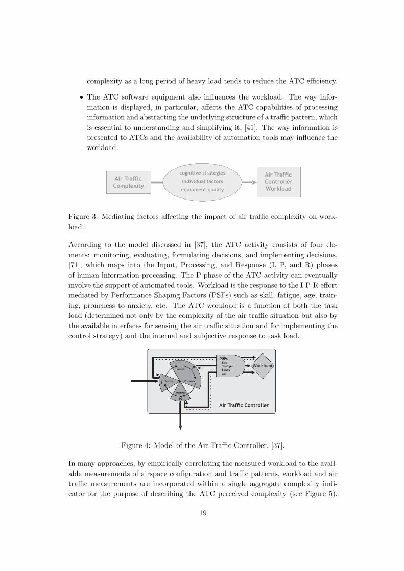
• The ATC software equipment also influences the workload. The way infor-mation is displayed, in particular, affects the ATC capabilities of processinginformation and abstracting the underlying structure of a traffic pattern, whichis essential to understanding and simplifying it, [41]. The way information ispresented to ATCs and the availability of automation tools may influence theworkload.

Figure 3: Mediating factors affecting the impact of air traffic complexity on work-load.

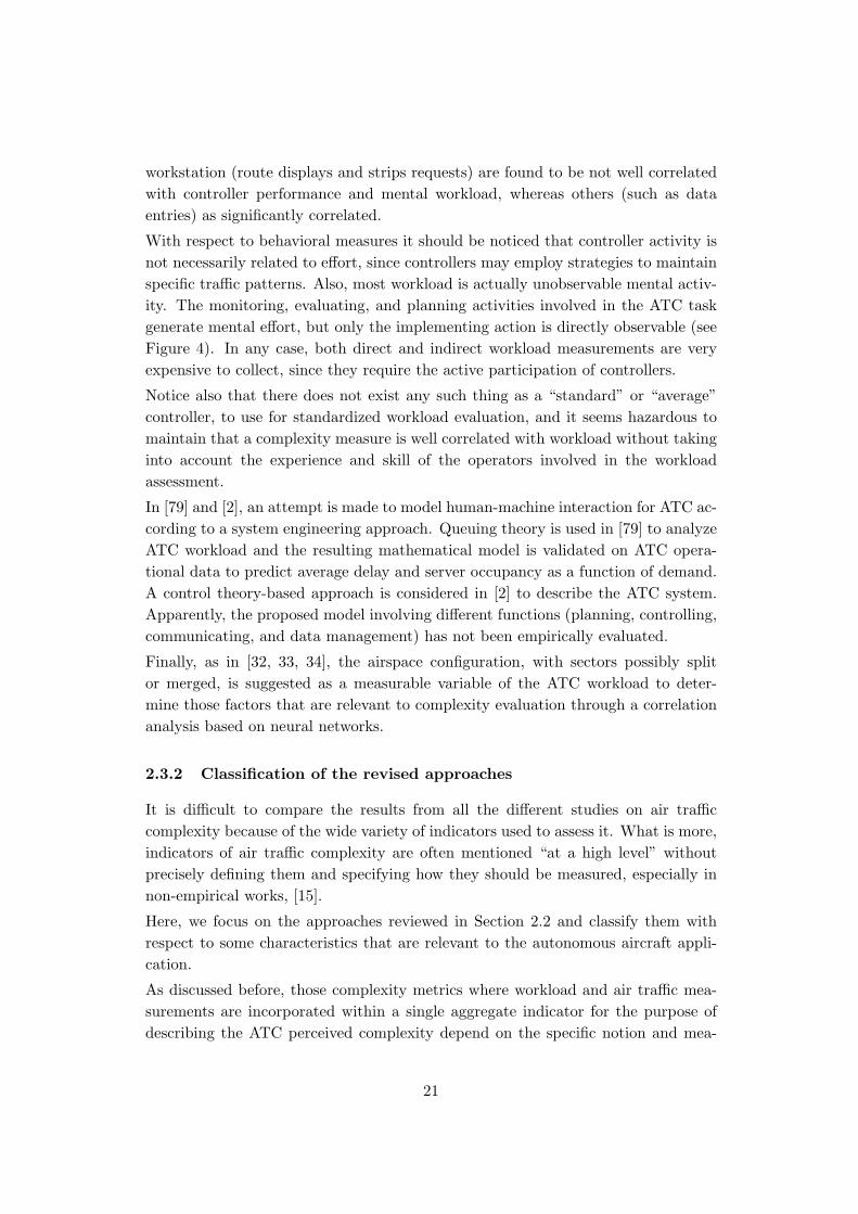
According to the model discussed in [37], the ATC activity consists of four ele-ments: monitoring, evaluating, formulating decisions, and implementing decisions,[71], which maps into the Input, Processing, and Response (I, P, and R) phasesof human information processing. The P-phase of the ATC activity can eventuallyinvolve the support of automated tools. Workload is the response to the I-P-R effortmediated by Performance Shaping Factors (PSFs) such as skill, fatigue, age, train-ing, proneness to anxiety, etc. The ATC workload is a function of both the taskload (determined not only by the complexity of the air traffic situation but also bythe available interfaces for sensing the air traffic situation and for implementing thecontrol strategy) and the internal and subjective response to task load.

Figure 4: Model of the Air Traffic Controller, [37].

In many approaches, by empirically correlating the measured workload to the avail-able measurements of airspace configuration and traffic patterns, workload and airtraffic measurements are incorporated within a single aggregate complexity indi-cator for the purpose of describing the ATC perceived complexity (see Figure 5).

19

While nearly all of the studies found a statistically significant correlation betweenair traffic factors and workload, not all airspace factors were related to the samemeasure of workload, which makes difficult to compare the different approaches toair traffic complexity. Clearly, the choice of the variable that measures the workloadis crucial to determine how well complexity is actually evaluated.

Figure 5: Complexity evaluation within ground-based ATM.

Workload can be measured using direct subjective indicators (such as self-reportmeasures and controller’s rating obtained through some questionnaire) or indirectindicators including behavioral/physical activity (e.g., key strokes, slew ball entries,number of control actions, communication time, decision and action frequency) andphysiological (e.g., EEG/EMG/EOG, blood pressure, heart rate measures, eye blinkrate, respiration, biochemical activity, pupil diameter) indicators. Various datacollection methods are listed in [37].

Workload is often indirectly and partially evaluated by measuring task performancesuch as time to perform discrete ATC tasks, [14]. In this way, the cognitive process(including planning, decision making, strategy, and factors such as skill, training, ex-perience, fatigue, etc.) of the controller is masked. A list of “workload indicators” isprovided in the literature review [37]. The issue of evaluating ATC performance andworkload based on data collected from operational and simulated air traffic controlis discussed in [75], where an extensive taxonomy of air traffic control measurementsadopted in the literature is provided.

Subjective measures suffer from several drawbacks, such as memory effects, un-willingness to report damaging information, etc (however, it should be noted thatworkload is –after all– a subjective reaction to traffic complexity). In [62, 63],the relevance of measures of the controller activity for realtime decision support isevaluated. Communications measures are found to be correlated with subjectiveworkload, but not to provide any incremental benefit when used for prediction ofits future behavior. Certain physical parameters related to the interaction with the

20

workstation (route displays and strips requests) are found to be not well correlatedwith controller performance and mental workload, whereas others (such as dataentries) as significantly correlated.

With respect to behavioral measures it should be noticed that controller activity isnot necessarily related to effort, since controllers may employ strategies to maintainspecific traffic patterns. Also, most workload is actually unobservable mental activ-ity. The monitoring, evaluating, and planning activities involved in the ATC taskgenerate mental effort, but only the implementing action is directly observable (seeFigure 4). In any case, both direct and indirect workload measurements are veryexpensive to collect, since they require the active participation of controllers.

Notice also that there does not exist any such thing as a “standard” or “average”controller, to use for standardized workload evaluation, and it seems hazardous tomaintain that a complexity measure is well correlated with workload without takinginto account the experience and skill of the operators involved in the workloadassessment.

In [79] and [2], an attempt is made to model human-machine interaction for ATC ac-cording to a system engineering approach. Queuing theory is used in [79] to analyzeATC workload and the resulting mathematical model is validated on ATC opera-tional data to predict average delay and server occupancy as a function of demand.A control theory-based approach is considered in [2] to describe the ATC system.Apparently, the proposed model involving different functions (planning, controlling,communicating, and data management) has not been empirically evaluated.

Finally, as in [32, 33, 34], the airspace configuration, with sectors possibly splitor merged, is suggested as a measurable variable of the ATC workload to deter-mine those factors that are relevant to complexity evaluation through a correlationanalysis based on neural networks.

2.3.2 Classification of the revised approaches

It is difficult to compare the results from all the different studies on air trafficcomplexity because of the wide variety of indicators used to assess it. What is more,indicators of air traffic complexity are often mentioned “at a high level” withoutprecisely defining them and specifying how they should be measured, especially innon-empirical works, [15].

Here, we focus on the approaches reviewed in Section 2.2 and classify them withrespect to some characteristics that are relevant to the autonomous aircraft appli-cation.

As discussed before, those complexity metrics where workload and air traffic mea-surements are incorporated within a single aggregate indicator for the purpose ofdescribing the ATC perceived complexity depend on the specific notion and mea-

21

sure of workload adopted, and inherently incorporate various human factors aspects.Also, such workload-oriented metrics are sector-based (in [29], reference is even di-rectly made to complexity of a sector as an estimate of the ATC workload of thatsector), and often show structural dependence on the sector characteristics, whichfurther limits their applicability to a sector-free context such as autonomous aircraftATM.

The various dynamic density-like metrics and the interval complexity are clearlyworkload-oriented and sector-based measures of complexity. The same holds for theaircraft density, since complexity is evaluated by comparing the number of aircraftin a sector with a threshold determined based on the capabilities of ATCs to safelyhandle air traffic in that sector.

The difficulty in obtaining reliable workload measures has been one of the strongestmotivations for investigating complexity metrics independent of the ATC workloadin the context of ground-based ATM. These metrics can be control-dependent orcontrol-independent, in that the evaluation of complexity can explicitly account forthe controller in place or not. The input-output model is a control-dependent metric,since complexity is evaluated in terms of control effort, whereas fractal dimensionand intrinsic complexity measures are control-independent. All workload-orientedmetrics are obviously control-dependent.

Control-independent metrics do not require the knowledge of the controller in place,which is indirectly accounted for through the effect of its action on the air traf-fic organization. This makes them better suited for the airborne self-separationframework.

Figure 6: Control scheme in autonomous aircraft ATM.

In autonomous aircraft ATM, control is delegated to the aircraft according to a par-tially decentralized control scheme where aircraft eventually communicate one withthe other (air-to-air communication) and with the ground (air-to-ground commu-nication) to get information on the other aircraft intent through the System WideInformation Management (SWIM) system, as schematically represented in Figure6. As a result, the controller has a decentralized time-varying structure, difficult to

22

characterize for the purpose of control effort evaluation, and possibly involving thepilots in the decisions on trajectory management and conflict resolution. A notion ofcomplexity explicitly accounting for a human-in-the-loop component would presentthe drawbacks that are common to all system engineering approaches applied tomodel human-machine interaction, that is:

i) Decision making or planning are generally unobservable processes and mea-surements are largely unreliable (due, e.g., to time varying human behaviorand to differences between individuals).

ii) Humans typically do not “optimize” but rather try to “satisfy” the require-ments, choosing a solution that is satisfactory though not necessarily the bestone. As a consequence, prediction of decision making processes is hard.

iii) Analytic modeling of human behavior is strictly related to the specific context(pervasiveness of task environment).

Thus, a control-independent measure of complexity appears to be the better suitedin view of the introduction of an airborne self-separation ATM system.

For those complexity measures that are computed based on the air traffic staterather than the whole aircraft trajectories, complexity prediction can be obtainedby projecting in the future the air traffic state and recomputing the complexitymeasure, whereas those measures that take into account the aircraft trajectoriesare naturally evaluating complexity over a prediction time horizon. In any case,the reliability of the resulting complexity prediction depends on that of the aircrafttrajectories prediction. Surprisingly, it seems that uncertainty in the trajectoryprediction is not accounted for in any of the (deterministic) approaches proposed inthe literature.

Depending on the reference time horizon, complexity metrics could be useful forconflict resolution or for trajectory planning (tactical and strategic decisions). In thisrespect, those approaches providing a spatial complexity map could help isolatingcritical areas and support trajectory management. The practical impact of thoseapproaches providing a scalar aggregate indicator of complexity is instead not soclear in most cases.

A further aspect that is interesting to point out is if and how the metric takes intoaccount the organization of traffic, which is recognized as an important factor in theassessment of complexity.

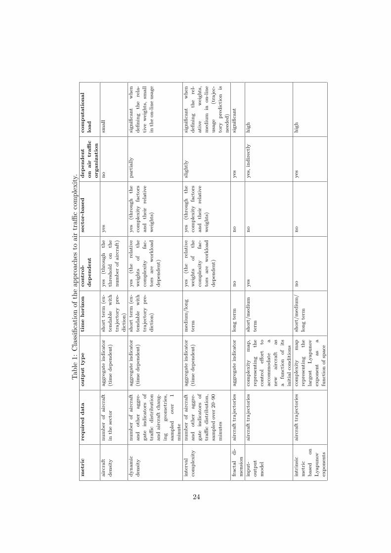
Table 1 is a schematic classification of the approaches reviewed in Section 2.2 basedon the aspects mentioned above, that is: the data required for complexity evaluation;the output provided; the reference time horizon; dependence on the controller, onthe sector, and on the traffic organization. A rough evaluation of the computationalload is also given, which is obviously an important information for the design of atime critical task such as air traffic management.

23

Tab

le1:

Cla

ssifi

cati

onof

the

appr

oach

esto

air

traffi

cco

mpl

exity.

metr

icrequir

ed

data

outp

ut

type

tim

ehoriz

on

contr

ol-

dependent

secto

r-b

ase

ddependent

on

air

traffi

c

organiz

ati

on

com

puta

tional

load

air

craft

den

sity

num

ber

of

air

craft

inth

ese

ctor

aggre

gate

indic

ato

r

(tim

edep

enden

t)

short

term

(ex-

tendable

wit

h

traje

ctory

pre

-

dic

tion)

yes

(thro

ugh

the

thre

shold

on

the

num

ber

ofair

craft

)

yes

no

small

dynam

ic

den

sity

num

ber

of

air

craft

and

oth

eraggre

-

gate

indic

ato

rsof

traffi

cdis

trib

uti

on

and

air

craft

chang-

ing

geo

met

ries

,

sam

ple

dover

1

min

ute

aggre

gate

indic

ato

r

(tim

edep

enden

t)

short

term

(ex-

tendable

wit

h

traje

ctory

pre

-

dic

tion)

yes

(the

rela

tive

wei

ghts

of

the

com

ple

xity

fac-

tors

are

work

load

dep

enden

t)

yes

(thro

ugh

the

com

ple

xity

fact

ors

and

thei

rre

lati

ve

wei

ghts

)

part

ially

signifi

cant

when

defi

nin

gth

ere

la-

tive

wei

ghts

,sm

all

inth

eon-lin

eusa

ge

inte

rval

com

ple

xity

num

ber

of

air

craft

and

oth

eraggre

-

gate

indic

ato

rsof

traffi

cdis

trib

uti

on,

sam

ple

dover

20–90

min

ute

s

aggre

gate

indic

ato

r

(tim

edep

enden

t)

med

ium

/lo

ng

term

yes

(the

rela

tive

wei

ghts

of

the

com

ple

xity

fac-

tors

are

work

load

dep

enden

t)

yes

(thro

ugh

the

com

ple

xity

fact

ors

and

thei

rre

lati

ve

wei

ghts

)

slig

htl

ysi

gnifi

cant

when

defi

nin

gth

ere

l-

ati

ve

wei

ghts

,

med

ium

inon-lin

e

usa

ge

(tra

jec-

tory

pre

dic

tion

is

nee

ded

)

fract

al

di-

men

sion

air

craft

traje

ctori

esaggre

gate

indic

ato

rlo

ng

term

no

no

yes

signifi

cant

input-

outp

ut

model

air

craft

traje

ctori

esco

mple

xity

map,

repre

senti

ng

the

contr

ol

effort

to

acc

om

modate

a

new

air

craft

as

afu

nct

ion

of

its

init

ialco

ndit

ions

short

/m

ediu

m

term

yes

no

yes

,in

dir

ectl

yhig

h

intr

insi

c

met

ric

base

don

Lyapunov

exponen

ts

air

craft

traje

ctori

esco

mple

xity

map

repre

senti

ng

the

larg

est

Lyapunov

exponen

tas

a

funct

ion

ofsp

ace

short

/m

ediu

m/

long

term

no

no

yes

hig

h

24

2.4 Concepts related to air traffic complexity

2.4.1 Trajectory flexibility

A concept that is intimately related to air traffic complexity is that of flexibility ofthe aircraft trajectory, i.e., the extent to which a trajectory can be modified withoutcausing a conflict with neighboring aircraft or entering a forbidden airspace area.

The use of flexibility measures in an airborne self separation framework is the objectof an ongoing research activity by NASA [44, 45, 43]. In the short/medium termflexibility is used as a criterion to rate different conflict resolution maneuvers, sothat the adopted solution is the easiest to adapt to unexpected behavior by intrudertraffic. In the long term horizon, a flexibility preservation function is adopted to planthe aircraft trajectory by minimizing its exposure to disturbances such as weathercells and dense traffic areas.

Flexibility is evaluated in terms of two different characteristics, namely robustnessand adaptability to disturbances. Robustness is defined as the ability of the air-craft to keep its planned trajectory unchanged in response to the occurrence of adisturbance, and is measured as the fraction of operationally feasible trajectoriesthat keep feasible. Adaptability is defined as the ability of the aircraft to changeits planned trajectory in response to the occurrence of a disturbance that makesthe current planned trajectory infeasible. Adaptability is measured as the amountof feasible trajectories that avoid the conflict while respecting all the navigationalconstraints.

The work [43] discusses computational aspects related to the actual computation ofsuch metrics in a probabilistic setting. Simplified scenarios are explored, where a 2Dspace is considered and only 1 degree of freedom (e.g., speed or path stretch) is an-alyzed at a time for trajectory modification. The concepts, however, are extendableto a more general setting.

2.4.2 Aircraft clustering

Aircraft clustering consists in identifying groups of closely spaced aircraft and wasoriginally studied in connection with conflict resolution. With reference to the con-flict resolution problem, clustering should isolate all the aircraft involved in multipleconflicts close in time and ensure that solving conflicts within each cluster separatelywill not generate any new inter-cluster conflict.

Assuming that aircraft density is a relevant factor for complexity characterization,[37, 54], cluster identification can complement and accelerate complexity assessmentby isolating those airspace areas where concentrating the attention. Once a highdensity area is identified by aircraft clustering, the following step is to evaluate itscomplexity, so as to eventually determine those critical airspace areas that should

25

be avoided.

Clusters play within the advanced autonomous ATM system a role similar to sectorswithin the centralized human-operated ATM system. Under current operations,airspace congestion refers to a sector that cannot accept additional aircraft dueto ATC workload limitations. In view of automated separation assurance, which isindependent of the airspace geometry, a methodology for identifying aircraft clustersis suggested in [7, 6] as a first step towards obtaining a sector-independent evaluationof the airspace congestion: aircraft clusters are isolated first and then congestion isevaluated based on cluster complexity.

We next briefly illustrate the main contributions in the literature on aircraft clus-tering, making the description uniform by adopting a common mathematical frame-work. No evaluation of which approach is best suited to support complexity evalu-ation in the autonomous aircraft case is given at this stage.

Let A be a set of aircraft in the airspace S ⊂ R3 of interest (in our case the self-separation enroute airspace), and T ⊂ R+ some reference time interval. The flightof aircraft a ∈ A can be described through some function pa = (xa, ya, za) : T → S,where pa(t) = (xa(t), ya(t), za(t)) represents the position of aircraft a at time t ∈ T .We denote by Ch,v

T ⊆ A×A the collection of aircraft pairs that get closer than somedistance specified in terms of horizontal and vertical separation, during the timeinterval T , i.e.

cab := (a,b) ∈ Ch,vT

m∃ts, tf ∈ T : de

((xa(t), ya(t)), (xb(t), yb(t))

)< h ∧ de(za(t), zb(t)) < v, ∀t ∈ [ts, tf ]

where de(w1, w2) denotes the Euclidean distance between vectors w1 and w2 andh, v are some positive constants.

Note that Ch,vT is a relation over A that is symmetric (if cab ∈ Ch,v

T then cba ∈ Ch,vT ,

a, b ∈ A) and reflexive (caa ∈ Ch,vT , ∀a ∈ A), but not transitive. The transitive

closure of Ch,vT allows to partition set A in equivalence classes, each class, say E =

{a, b, c}, corresponding to a cluster of aircraft that get close one to the other directly(cab ∈ Ch,v

T ) or indirectly ( cac, ccb ∈ Ch,vT but cab 6∈ Ch,v

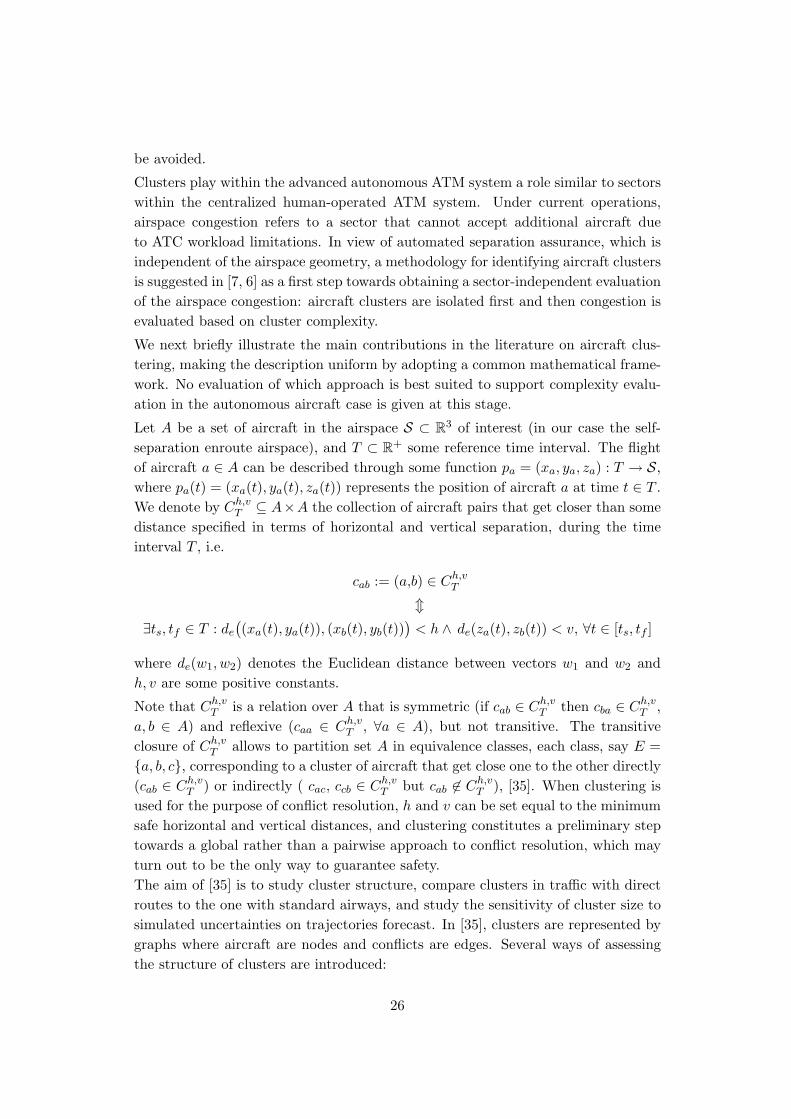
T ), [35]. When clustering isused for the purpose of conflict resolution, h and v can be set equal to the minimumsafe horizontal and vertical distances, and clustering constitutes a preliminary steptowards a global rather than a pairwise approach to conflict resolution, which mayturn out to be the only way to guarantee safety.The aim of [35] is to study cluster structure, compare clusters in traffic with directroutes to the one with standard airways, and study the sensitivity of cluster size tosimulated uncertainties on trajectories forecast. In [35], clusters are represented bygraphs where aircraft are nodes and conflicts are edges. Several ways of assessingthe structure of clusters are introduced:

26

• the number of nodes;

• the number of edges;

• the diameter of the graph of the cluster;

• the graphic sequence

The graphic sequence is defined as a sequence of numbers that can be the degreesequence of a graph (a degree of a node is the number of attached edges).The paper first presents how structure variability (in terms of graphic sequences)grows with the number of aircraft in a cluster. Then the two scenarios (traffic withdirect routes and traffic with standard airways) are simulated with the conclusionthat direct routes traffic results in less conflicts. On the other hand, the clusterdiameter as a function of the number of aircraft is slightly larger for direct routesscenario. Experiments with added uncertainty showed that more clusters are de-tected, therefore a good trajectory prediction/knowledge is needed in order not tooverwhelm the conflict resolution module.

The disadvantage of this approach is that if aircraft a and b are close up to timetf (cab) and then b and c start being close at ts(cbc), all three aircraft belong to thesame cluster, even if |ts(cbc) − tf (cab)| is relatively big. To solve this issue, a newrelation ρ is introduced in [16] for expressing the temporal proximity of conflictsdefined by the relation Ch,v

T :

cab ρ cbc ⇔ mint′∈[ts(cab),tf (cab)],t

′′∈[ts(cbc),tf (cbc)]|t′ − t

′′ | < ∆

where ∆ ∈ R represents a time threshold.Each cluster of aircraft corresponds to one equivalence class of the transitive closureof the proximity relation ρ. A cluster corresponding to the equivalence class withrepresentative cab, denoted as [cab]ρ, is built by the union of all aircraft in it, i.e. as

⋃

(r,s)∈[cab]ρ

{r, s}

Note that in this case clusters do not have to be disjoint, and time specificationis therefore needed, e.g., an aircraft can be part of a given cluster only within aspecified time interval.

In [8], clusters are built as equivalence classes of aircraft where the equivalence isthe transitive closure of the relation Ch,v

T for T = {t∗}, for each fixed discretizedtime instant t∗ in some look-ahead time horizon. Clusters with less than 5 aircraftare not taken into account, and such aircraft are put in so-called background traffic.

Project MAICA (Modelling and Analysis of the Impact of the Changes in ATM –briefly described in [73]) aimed at evaluating the impact of several changes in ATM(including autonomous aircraft) to ATM performance.

27

The definition of cluster in this project is rather vague (unfortunately, reports arenot available, and all information is extracted from other reviews and references).Similarly to [16], aircraft clusters are built based on a proximity relation, which,however, considers both the temporal and spatial proximity of aircraft pairs definedby relation Ch,v

T . The idea is that aircraft a, b and aircraft c, d with cab, ccd ∈ Ch,vT

should belong to the same aircraft cluster only if the event where a and b get close oneto the other (which is the reason why cab ∈ Ch,v

T ) is both spatially and temporarilyclose to the event where c and d get close one to the other. Neither in this case theaircraft clusters have to be disjoint, therefore a time specification of the inclusion ofan aircraft into a given cluster may be needed.

It is worth also mentioning the fact that innovative cluster definitions are proposedin the Master thesis of G. Aigoin, which is not available, but whose contribution isbriefly described in [23].

28

3 A dynamical approach to intrinsic air traffic complex-

ity characterization

As discussed in Chapter 2, air traffic complexity has been typically studied withthe objective of quantifying the workload of air traffic controllers in handling airtraffic. The workload of a controller is determined by two aspects: an intrinsiccomplexity related to the air traffic structure, and a subjective component relatedto the controller himself/herself (cognitive strategies and individual characteristics).Most complexity metrics proposed in the literature aim at capturing both theseaspects within a single aggregate indicator of “perceived complexity”. A measureof the intrinsic air traffic complexity aspect only is instead needed within a highlyautomated ATM system.

Site visits to air traffic facilities and a review of previously identified complexityfactors suggests that organization in the distribution of aircraft positions and speedscan have an important effect on the perceived complexity of the traffic situation [39].In particular, situations where the relative distances between aircraft do not changeover time are more predictable and easier to control. These situations are classifiedas fully organized traffic. On the other hand, quasi-random situations are difficultto handle and are thus associated with high complexity.

In this section we describe a dynamical approach to complexity characterization: acomplexity indicator which quantifies the level of organization of the air traffic isintroduced by using tools borrowed from the theory of dynamical systems.

3.1 The underlying principle

In order to capture the complexity associated to a lack of organization, an air trafficsituation can be modeled by an evolution equation, with the aircraft trajectoriesinterpreted as integral lines of some dynamical system. The Lyapunov exponents ofthe dynamical system provide an indicator of the air traffic complexity, allowing forthe identification of different organizational structures of the aircraft speed vectorssuch as translation, rotation, divergence, convergence, or a mix of them. Lyapunovexponents are a standard complexity measure adopted in dynamical systems theory.They are the natural generalization to time dependent linear differential equations ofthe eigenvalues for autonomous linear systems and characterize the growth rates ofthe solution. For systems described by nonlinear differential equations, they measurethe rate of exponential convergence or divergence of nearby trajectories, and canbe taken as indicators of the level of order/disorder of a system. Quantitatively,two trajectories with initial relative position δx0 diverge as eλt‖δx0‖, where λ is aLyapunov exponent. The rate of separation can be different for different orientationsof the initial separation vector δx0. Thus, there is a whole spectrum of Lyapunovexponents. The number of Lyapunov exponents is upper bounded by the dimension

29

of the state space of the dynamical system. The value taken by the Lyapunovexponents at a certain position represents the local contraction/expansion rate ofthe field. The larger is a positive Lyapunov exponent, the higher is the rate at whichone loses the ability to predict the system response. Those areas where the traffic ispredictable are then easily identified by plotting the air traffic complexity map thatis the largest Lyapunov exponent as a function of the airspace position.

The claim is that high air traffic complexity is associated with high Lyapunov ex-ponents.

The part which follows is largely taken from the draft paper [74] by S. Puechmorelunder the iFly project. For more details on Lyapunov exponents, the reader isreferred to [5].

3.2 Lyapunov exponents as complexity indicator

3.2.1 Definition and properties

We start by recalling some basic notions of dynamical system theory.

Definition 1 Let M ⊆ <n be a smooth manifold. A flow on M is a mappingψ : <×M→M such that:

• ψ(0, x) = x, ∀x ∈M;

• ψ(t + s, x) = ψ(t, ψ(s, x)), ∀x ∈M, ∀s, t ∈ <.

The pair (M, ψ) constitutes a continuous time dynamical system with state spaceM, and x(·) = ψ(·, x0) : < → M is the trajectory associated with x0 ∈ M, i.e.,such that x(0) = x0.

Remark 1 We restrict here our attention to continuous time systems described byflows, which are the objects of interest for our complexity application; however, it ispossible to extend the discussion to discrete time systems resulting in iterated maps.Most of the time extra assumptions are made on the flow. For example, measur-ability (resp. continuity) with respect to the couple (t, x) yields measurable (resp.continuous or topological) flows. Smoothness assumptions are generally made withrespect to the state space variable x only: a flow is of class Ck if the mappingψ(t, ·) : M→M is differentiable up to order k and the resulting derivative ψ(k) iscontinuous as a mapping <×M→M. The two previous properties are often calledcocycle properties.

According to Definition 1, flows are two-sided in time, i.e., it is possible to setarbitrary values for time t. Very often however, flows are implicitly defined by adifferential equation and fail to be defined at every time or everywhere on M. To

30

cope with this situation, the relaxed notion of local flow is introduced. The onlyimportant modification to the definition is that ψ is a mapping from D ⊂ <×M→M, satisfying the cocycle conditions and with the domain D such that:

• D is open, non void;

• Dx = {t ∈ <|(t, x) ∈ D} is an open interval containing 0, for any x ∈M;

• t ∈ Dψ(s,x) if and only if t + s ∈ Dx.

With the previous notation, Dx = {τ−(x), τ+(x)}, where τ+(x) (τ−(x)) is the for-ward (backward) explosion time of the trajectory starting at x at time t = 0. Adynamical system will be defined in the following by a local flow. The domain Dis assumed to be implicit from the differential equation generating the flow unlessotherwise noted.

Consider a system governed by the linear differential equation x(t) = Ax(t) in <n.The behavior of x(t) as time grows to infinity can be derived from the eigenvaluesof A. However, even by relaxing only the fact that the system is autonomous (i.e.x(t) = A(t)x(t)) this simple approach breaks down and knowing the eigenvaluesof A(t) is of little help to understand the asymptotic behavior of the system. Itturns out that the right definition is a kind of local shear factor called the Lyapunovexponents. We shall start by introducing Lyapunov exponents for the linear systemdescribed by x(t) = A(t)x(t). Lyapunov exponents for x(t) = A(t)x(t) play thesame role in asymptotic stability analysis as the real parts of the eigenvalues of A

for x(t) = Ax(t), and in fact they are given by the real parts of the eigenvalues ofA in this case. The considerations developed in the linear time-varying setting willbe useful when dealing with nonlinear systems.

Let x(t) = φ(t)x be the solution of the non autonomous linear differential equa-tion x(t) = A(t)x(t) initialized with x(0) = x. The (forward) Lyapunov exponentassociated with x ∈ <n is defined as:

λ(x) = lim supt→+∞

1t

log ‖φ(t)x‖

One can define similarly the backward Lyapunov exponent by considering φ(−t)xinstead of φ(t)x. Conventionally, λ(0) = −∞.

Remark 2 In numerical analysis, Lyapunov exponents are studied to quantify thesensitivity to the initial condition of the solution to a differential equation. In-deed, the Lyapunov exponent λ(x) measures the mean (exponential) rate of conver-gence/divergence of two trajectories with initial relative position δx(0) = x. Notein fact that δx(t) = φ(t)x represents the evolution in time of the distance between thetwo trajectories, so that λ(x) = lim supt→+∞

1t log ‖δx(t)‖ = lim supt→+∞

1t log ‖δx(t)‖

‖x‖is such that ‖δx(t)‖ ' eλ(x)t‖x‖.

31

Proposition 1 Let x, y ∈ <n be such that λ(x) 6= λ(y). Then, x and y are linearlyindependent.

Proof: The proposition can be easily established by first showing two simpleproperties of Lyapunov exponent. First, let a 6= 0 be a real number. Then:

λ(ax) = lim supt→+∞

1t

log ‖φ(t)ax‖ = lim supt→+∞

1t

(log ‖φ(t)x‖+ log(|a|)

= lim supt→+∞

1t

log ‖φ(t)x‖ = λ(x)

Now, consider two vectors x and y. Since ‖φ(t)(x + y)‖ ≤ 2max(‖φ(t)x‖, ‖φ(t)y‖),we have

λ(x + y) = lim supt→+∞

1t

log ‖φ(t)(x + y)‖ ≤ max(λ(x), λ(y))

From this it can be deduced that if λ(x) > λ(y), then

λ(x + y) ≤ λ(x) ≤ max(λ(x + y), λ(−y))

and since λ(x) > λ(y) the max in the right hand side must be λ(x + y) so thatfinally if λ(x) 6= λ(y), then

λ(x + y) = max(λ(x), λ(y))

Now we are ready to prove the proposition since if x and y are two non zero vectorssuch that λ(x) 6= λ(y), then if ax + by = 0, λ(0) = −∞ = max(λ(x), λ(y)), whichin turn implies that a = b = 0.

It is interesting to note that the previous result is obtained by using only the fol-lowing three fundamental properties of a Lyapunov exponent function λ : <n →<∪ {−∞}

• λ(ax) = λ(x), for any x ∈ <n and a ∈ < \ {0};

• λ(x + y) ≤ max(λ(x), λ(y)), for any x, y ∈ <n, with equality holding if λ(x) 6=λ(y)

• λ(0) = −∞ (normalization condition)

Functions satisfying these requirements are called characteristic exponents and sharemost of the salient features of Lyapunov exponents. From the linear independence ofvectors with different Lyapunov exponents, it is clear that there exists only a finitenumber p ≤ n of Lyapunov exponents λ1, λ2, . . . , λp. Assuming that the exponentsare ordered λ1 < λ2 < · · · < λp, we can construct a filtration {0} = V0 ⊂ V1 ⊂V2 ⊂ · · · ⊂ Vp = <n of <n such that λ(x) = λi for x ∈ Vi \ Vi−1. The multiplicity

32

of λi is the number ki = dimVi − dimVi−1. A basis {e1, e2, . . . , en} of <n is normal(ordered) with respect to the filtration if there exists an increasing sequence ni,,i = 1, 2, . . . , p, such that {e1, e2, . . . , eni} form a basis of Vi for all i = 1, 2, . . . , p. Anormal basis {e1, e2, . . . , en} is characterized by the fact that:

n∑

i=1

λ(ei) = inf{ n∑

i=1

λ(fi), {f1, f2, . . . , fn} basis of <n}

For Lyapunov exponent computations, we need some extra work on orthogonalityrelations.

Let <n be considered as it own dual with pairing 〈·, ·〉. Let {e1, e2, . . . , en} and{f1, f2, . . . , fn} be two dual bases, that is 〈ej , fi〉 = δi,j , ∀i, j = 1, 2, . . . , n. Considernow a characteristic exponent function γ : <n → < ∪ {−∞} defined by the threeproperties mentioned before. Let Γ = {γi, i = 1, . . . , n} be the characteristic expo-nents associated to {e1, e2, . . . , en} (i.e. γi = γ(ei)) and Γ′ = {γ′i, i = 1, . . . , n} bethe characteristic exponents associated to {f1, f2, . . . , fn} (i.e. γ′i = γ(fi)).

Definition 2 The sets of characteristic exponents Γ, Γ′ are said to be dual if γi +γ′i ≥ 0, ∀i = 1, 2, . . . , n.

For dual characteristic exponents, we can define the regularity coefficient

Definition 3 The regularity coefficient κ(Λ, Λ′) of the dual characteristic exponentsΓ,Γ′ is

κ(Γ,Γ′) = minmax{γi + γ′i, i = 1, . . . , n}

where the minimum is computed over all possible pairs of basis in duality.

One can check that dual Lyapunov exponents have a positive regularity coefficient.

Definition 4 Dual characteristic exponents Γ, Γ′ are said to be regular if κ(Γ, Γ′) =0.

Proposition 2 Let Γ, Γ′ be regular exponents. The filtrations associated with Γ andΓ′ are mutually orthogonal.

If the filtration {0} = V0 ⊂ V1 ⊂ V2 ⊂ · · · ⊂ Vp = <n is associated with Γ and{0} = W0 ⊂ W1 ⊂ W2 ⊂ · · · ⊂ Wq = <n with Γ′, orthogonality between the twofiltrations means that

• p = q

• dimVi + dim Wp−i = n, ∀i = 0, 1, . . . , p

• Vi ⊥ Wp−i, ∀i = 0, 1, . . . , p

33

The dual equation of the non autonomous linear differential equation x(t) = A(t)x(t)is given by

y(t) = −AH(t)y(t)

where AH(t) is the Hermitian conjugate of A(t). By simple computations:

d

dt〈x(t), y(t)〉 = 〈A(t)x(t), y(t)〉+ 〈x(t),−AH(t)y(t)〉

= 〈A(t)x(t), y(t)〉 − 〈A(t)x(t), y(t)〉 = 0

so that orthogonality is preserved if x(0) and y(0) are orthogonal. Taking dual basesof <n, it can be proven that the Lyapunov exponents Λ associated with the originalequation and Λ′ associated with the dual equation are dual. The original system issaid to be regular if Λ and Λ′ are regular.Now we formulate the key theorem for the computation of the Lyapunov exponentsunder the assumption of regularity of the system.

Theorem 1 If the system described by x(t) = A(t)x(t) is regular, then, for anynormal ordered basis {e1, e2, . . . , en} and any k = 1, 2, . . . , n:

limt→+∞

1t

log | det Gk(t)| = 2k∑

i=1

λ(ei) (1)

where Gk(t) is the Gram matrix formed from the inner products: [Gk(t)]i,j =〈ei(t), ej(t)〉, i, j = 1, . . . , k, and ei(t) the solution of the differential equation withinitial condition ei(0) = ei.

The Gram matrix Gk(t) can be obtained from the normal fundamental matrix so-lution to x = A(t)x, that is the matrix E(t) satisfying the differential equationE(t) = A(t)E(t) with initial condition E(0) given by the matrix with the vectors{e1, e2, . . . , en} of the normal basis on the columns. Lyapunov showed that a nor-mal basis always exists and how it can be constructed from a fundamental matrixsolution, [25].

It is worth noting that in equation (1) we have a standard limit instead of the lim supas in the definition of Lyapunov exponents, and that the determinant of the Grammatrix is the square of the volume of the parallelepiped spanned by the vectorse1(t), . . . , ek(t), so that Lyapunov exponents can be viewed as local rates of growth.

Lemma 1 Let Q : < → GLn be a smooth mapping with value in the linear groupof dimension n. The change of variable y(t) = Q−1(t)x(t) results in the equation:

y(t) = M(t)y(t)

with M(t) = Q−1(t)(A(t)Q(t)− Q(t))

34

The proof of this lemma is straightforward.

Lemma 2 There exists a smooth change of variables Q with values in the unitarymatrices such that matrix M(t) = Q−1(t)(A(t)Q(t)− Q(t)) in the previous equationis upper triangular.

Proof: Let {e1, . . . , en} be a basis of <n and let ei(t), i = 1, . . . , n, be the solutionof the equation x(t) = A(t)x(t) with initial condition ei(0) = ei. Let Q(t)R(t) bethe QR-decomposition of the matrix E(t) with columns {e1(t), . . . , en(t)}. SinceE(t) = A(t)E(t), i.e., E(t) is a fundamental solution matrix for x = A(t)x, we have

R(t) = (QH(t)A(t)Q(t)−QH(t)Q(t))R(t) = M(t)R(t)

Given that the solution R(t) to this differential equation has to be upper triangular,then, matrix M(t) must be upper triangular as claimed.

This lemma from Perron is the key ingredient in the proof of the main theorem.Moreover, it is interesting in its own right and thus has been included. Perron’slemma is in fact adopted in nearly all numerical algorithms for computing the k

largest Lyapunov exponents by temporal integration. Lyapunov exponents are in-variant with respect to the smooth change of coordinates by the unitary matricesQ(t) (since it satisfies the norm-preserving property), [24]. Moreover, regularity ispreserved under such transformation, [24].

Consider the nonlinear system described by the differential equation:

x(t) = X(x(t))

and denote the corresponding flow by ψ. Consider the trajectory x(t) = ψ(t, x0)associated with x(0) = x0. The Lyapunov exponents are a characterization of theasymptotic properties of the solution ψ(t, x0) via analysis of the linearized problem.The linear approximation of the system around ψ(t, x0) is given by

δx(t) = A(t, x0)δx(t)

where Ax0(t) := DxX(x)|x=ψ(t,x0) with Dx denoting the derivative with respect tothe x variable. Matrix A(t, x0) of the linear approximation describes the instanta-neous rate of shearing of the infinitesimal neighborhood of x(t) = ψ(t, x0).

From the Taylor expansion of the flow:

δx(t) := ψ(t, x0 + δx0)− ψ(t, x0) = Dx(ψ(t, x))|x=x0δx0 + . . .

it follows that the deformation of an infinitesimal neighborhood of the initial con-dition after the time interval t is given by Dx(ψ(t, x0)) := Dx(ψ(t, x))|x=x0 , whichrepresents the shearing after a finite time t. Its eigenvalues and eigenvectors describe

35

deformation of an initial infinitesimal sphere of neighboring trajectories into an el-lipsoid time t later. Nearby trajectories separate exponentially along the unstabledirections and approach each other along the stable directions.

The Lyapunov exponent at x0 associated with x is defined as

λx0(x) = lim supt→+∞

1t

log ‖Dx(ψ(t, x0))x‖ (2)

and describes the mean exponential rate of divergence/convergence of the trajectoryobtained by a perturbation δx0 = x of the initial state x0 (lim supt→+∞

1t log ‖δx(t)‖

‖δx0‖ )computed based on the linear approximation.

Under standard regularity assumptions on X:

d

dtDx(ψ(t, x0)) = Ax0(t)Dx(ψ(t, x0))

with Dx(ψ(0, x0)) = I. Thus Dx(ψ(t, x0)) can be viewed as a fundamental solu-tion matrix for the linear differential equation y(t) = Ax0(t)y(t), which makes thediscussion on the linear case useful also in the nonlinear setting of interest.

It is worth noting that Dxψ(t, x0) defines a linear cocycle over the flow ψ.

Definition 5 Let (M, ψ) be a dynamical system where ψ is a local flow with domainD. A linear (invertible) cocycle over ψ is a mapping S : D → GL(<) such that:

• S(0, x) = I, ∀x ∈M;

• S(t + s, x) = S(s, ψ(t, x))S(t, x), ∀x ∈M, ∀t, s ∈ <.

For a linear cocycle S(t, x), the associated Lyapunov exponents are defined as:

λx = lim supt→+∞

1t

log ‖S(t, x)‖ (3)

where ‖S(t, x)‖ is the norm of matrix S(t, x) induced by the 2-norm for vectors(largest singular value) or, equivalently, the square root of the maximum eigenvalueof the positive definite symmetric matrix S(t, x)T S(t, x).

According to the definition (2) of Lyapunov exponents of the dynamical systemx(t) = X(x(t)) at x0, equation (3) with x = x0 provides the largest Lyapunovexponent of the dynamical system at x0 when applied to the linear cocycle S(t, x0) =Dxψ(t, x0).

3.2.2 Computational aspects

Numerical pitfalls. Computing Lyapunov exponents amounts to integrate a dif-ferential equation, giving the linear cocycle S(t, x0) = Dxψ(t, x0). Nearly all stan-dard algorithms can be used for that purpose but one quickly realize that the prob-lem is far from being well conditioned. In fact, most of the time it is easy to obtain

36

the flow ψ(t, x) (needed for computing matrix Ax0(t)) with good accuracy but byconstruction S(t, x0) tends to grow exponentially fast in some directions (corre-sponding to positive Lyapunov exponents) and to decay exponentially fast in others(corresponding to negative Lyapunov exponents), thus giving a condition numberincreasing again exponentially. For this reason, it would be extremely inaccurateto compute Lyapunov exponents by merely integrating the linear cocycle, and somekind of rescaling is needed to recover good numerical properties. There is abun-dant literature on the subject, however all methods fall into one of two categories,i.e. spatial integration or temporal integration. Direct application of the definitiongives the second approach while the ergodic theorem gives the first one. Both haveadvantages and drawbacks:

• Spatial integration is efficient and free from the slow convergence phenomenonoccurring sometimes in temporal integration. However, in order to use theergodic theorem, one must find an invariant measure. Most of the time, it hasto be done by covering algorithms.

• Temporal integration can suffer from slow convergence. Moreover, it requiresperiodic rescaling to avoid numerical problems.

In the complexity application, only the temporal approach has been tested.

Algorithms based on differential geometry. All the machinery used in thispart is borrowed from the journal paper [12] by T.J. Bridges and S. Reich. Basically,the trick is to use Lemma 2 and Theorem 1 to compute the k largest Lyapunovexponents. The problem reduces then to continuously update the QR factorization(or a polar decomposition which is very similar except that the right hand side matrixis symmetric instead of being upper triangular). The differential equation satisfiedby Q can be established by noticing first that the matrix M(t) = QH(t)A(t)Q(t)−QH(t)Q(t) is upper triangular, so that adding its conjugate yields a symmetricmatrix with the same coefficients except on the diagonal where they are doubled.However,

MH(t) + M(t) = QH(t)(A(t) + AH(t))Q(t)

since QH(t)Q(t)+QH(t)Q(t) = 0 (Q(t) is unitary so the derivative of QH(t)Q(t) = I

vanishes). This implies that M(t) can be obtained without the knowledge of Q(t).Now, simply use the relation:

Q(t) = A(t)Q(t)−Q(t)M(t)

This differential equation can be solved readily by standard Runge-Kutta integra-tion. However, the orthogonality of Q is hard to preserve, so that efficient imple-mentations require specific algorithms. A natural approach is to use integrators

37

working on the Stiefel manifold on which Q lives. We refer to the previously men-tioned paper for details. It seems possible (although not implemented yet) to usethe Levi-Civita connection on the flag manifold to obtain closely related algorithm,but enforcing the fact that there is filtration adapted to Lyapunov exponents. Thecurrently used algorithm for computing Lyapunov exponents is the continuous polardecomposition updating.

3.3 Modelling air traffic as a dynamical system

Observed aircraft trajectories constitute only a finite set of the possible integral linesof the system, hence some extra assumptions are needed to determine a dynamicalsystem describing the air traffic situation under consideration. Appropriate smooth-ness conditions are required to ensure that the solution to the problem is unique.More precisely, given the aircraft velocities vi, i = 1, 2, . . . , N , at the measurementpoints xi, i = 1, 2, . . . , N , we determine the autonomous nonlinear dynamical systemdescribed by

x(t) = X(x(t)),

by using vector spline interpolation to fit the vector field X : <3 → <3 to theavailable interpolation data {(xi, vi), i = 1, 2, . . . , N}. Vector field X must satisfythe interpolation constraints X(xi) = vi, i = 1, 2, . . . , N , while minimizing thesmoothness div-curl energy functional. If X is a vector field of class at least C2,then, the div-curl energy of X in the domain U ⊂ <3 is given by:

E(X) =∫

Uα‖∇divX(x)‖2 + β‖∇curlX(x)‖2dx

where divX and curlX respectively denote the divergence field and the rotationalfield of the vector field X, ∇ is the gradient operator, and α and β are positivereal numbers controlling the relative weight of smoothness imposed on variations ofthe divergence field and the rotational field, respectively. It is a well known resultin spline theory that the vector field X minimizing E(X) under the constraintsX(xi) = vi, i = 1, 2, . . . , N is of the form :

X(x) =N∑

i=1

ciψ(x− xi) + θ(x)

where θ(x) = Ax+b is an element of the kernel of the differential operator consideredin the energy functional and ψ is the elementary solution of the operator P :

P = αdivT∇T∇div + β curlT∇T∇curl

If α is much greater than β, the optimal vector field X will tend to have a nearlyconstant divergence, while if β is much greater than α, the curl will be nearly

38

constant. An interesting special case occurs when α = β.When α = β, P reduces to ∆2 and ψ is the biharmonic kernel on all three coordinateswhich becomes independent. The corresponding splines are the well known thin-plate splines. Thus in the case of α = β, the vector spline problem is convertedinto three separated scalar thin-plate spline problems, which causes a dramaticdecrease in computation. The drawback is that the thin-plate spline deals with thecomponents of a vector independently, hence the interpolating vector field does notpreserve possible significant correlations between them. The procedure describedabove can be extended to time-dependent vector fields with a slight modificationof energy functional. In a case of short time periods (say around 10 sampled orforecasted positions on each trajectory) it is possible to compute an interpolatingvector field for 5000 aircraft within 10 minutes.

39

4 Conclusions and future work

Based on the review of the studies in the literature on air traffic complexity, we canconclude that

• most complexity metrics are strictly related to the current ground-based ATMsystem, where ATCs are in charge of guaranteeing safety in air traffic, andcannot be extended to the autonomous aircraft context because they incorpo-rate a measure of workload and often strongly dependent on the sector-basedairspace structure;

• those metrics that do not incorporate the measured workload but dependexplicitly on the controller in place are difficult to apply to the autonomousaircraft context because of the decentralized time-varying structure of thecontrol in the self-separation airspace, possibly involving a human in the loopcomponent;

• those approaches providing a single aggregate indicator of complexity oftenlack of an operational interpretation;

• approaches providing local information through a complexity map may beuseful for trajectory management by isolating critical areas that should beavoided;

• in view of the above considerations, the approaches in the literature thatappear more portable to the autonomous aircraft context are those providinga measure of intrinsic complexity of air traffic;

• the time dependence aspect should be better focused, introducing approachesto air traffic complexity evaluation specific for the long term (trajectory man-agement) and the short/mid term (conflict detection and resolution), eventu-ally accounting for uncertainty in the aircraft trajectory prediction.

Our plan for the future work under WP3.2 is

i) specify the requirements on complexity metrics for the iFly A3 Concept ofOperations defined in work package 1;

ii) further develop the dynamic approach to intrinsic air traffic complexity char-acterization described in Chapter 3;

iii) study alternative complexity metrics tailored to the short/medium term andto the long term.

40

Regarding the development of alternative complexity metrics, some preliminaryideas are as follows.

As for the long term, the goal is to allow for the identification of critical areas thatshould be possibly avoided. Aircraft density will be a relevant factor jointly with itsevolution in time. Evaluation of complexity will be based on the intended aircrafttrajectories, with the understanding that each aircraft should generally conform toits current intent information. Complexity will be recomputed from time to time totake care of possible modifications of the aircraft intent. Unexpected deviations at afiner time scale will be accounted for by the short/medium term complexity metric.Since complexity will be evaluated based on the intent information and currentstate of all aircraft in the self-separation airspace, it may be more convenient toperform computations on the ground and distribute only the (compact) descriptionof the critical areas to aircraft, rather than performing computations on-board ofall aircraft. Indications on how to set a generally applicable threshold to distinguishbetween low and high complexity areas will be provided. This is actually a criticalaspect for the intrinsic complexity measure described in Chapter 3.

As for the short/medium term, the goal is to identify air traffic encounters thatcould generate situations of conflict difficult to solve based on air traffic measure-ments only, without directly referring to the adopted resolution methodology. Away of achieving this is to evaluate complexity in terms of availability of feasibleresolution maneuvers for accommodating an additional aircraft entering the airspaceregion or for solving conflicts due to deviations of the aircraft from their plannedtrajectory: the larger is the solution space, the lower is complexity. Most likely aprobabilistic approach will be taken.In contrast with the input-output model in Section 2.2.5 where complexity is mea-sured as the control effort required for implementing a specific optimal conflictresolution strategy, the idea is that complexity should be measured as the effortrequired for determining a feasible, not necessarily optimal, resolution maneuver.This makes complexity evaluation independent of the adopted optimality criterion.The research on trajectory flexibility, related to the aircraft manoeuvrability and toits capability of accommodating unexpected disturbances, and that on probabilisticconflict/collision prediction [72, 42, 10, 9] might turn out to be useful for developingthis approach.

41

References

[1] RTCA Task Force 3. Free flight implementation. Technical report, RTCA Inc.,October 1995.

[2] V.R. Hunt ad A. Zellweger. Strategies for future air traffic control systems.Computer, pages 19–32, 1987.

[3] B.A. Arad. The controller load and sector design. Journal of Air Traffic Control,pages 12–31, 1964.

[4] S. Athenes, P. Averty, S. Puechmorel, D. Delahaye, and C. Collet. Complexityand controller workload: Trying to bridge the gap. In International Conferenceon Human-Computer Interaction in Aeronautics, HCI-Aero, Cambridge (MA),USA, 2002.

[5] Luis Barreira and Yakov B. Pesin. Lyapunov Exponents and Smooth ErgodicTheory. Number 23 in University Lecture Series. American Mathematical So-ciety, 2002.

[6] K. Bilimoria and M. Jastrzebski. Properties of aircraft clusters in the nationalairspace system. In AIAA Aviation Technology, Integration and OperationsConference (ATIO), number AIAA 2006-7801, Wichita, Kansas, September2006.

[7] K. Bilimoria and H. Lee. Analysis of aircraft clusters to measure sector-independent airspace congestion. In AIAA Aviation Technology, Integrationand Operations Conference (ATIO), number AIAA 2005-7455, Arlington, VA,September 2005.

[8] K.D. Bilimoria and M. Jastrzebski. Aircraft clustering based on airspace com-plexity. 7th AIAA Aviation Technology, Integration and Operations Conference,2007.

[9] H.A.P. Blom, G.J. Bakker, and J. Krystul. Probabilistic reachability analysisfor large scale stochastic hybrid systems. In 46th IEEE Conf. on Decision andControl, 2007.

[10] H.A.P. Blom, J. Krystul, and G.J. Bakker. A particle system for safety verifi-cation of free flight in air traffic. In 45th IEEE Conf. on Decision and Control,2006.

[11] A.L. Breitler, M. Lesko, and M. Kirk. Effects of sector complexity and controllerexperience on probability of operational errors in air route traffic. TechnicalReport DTFA01-95-C-00002, FAA, 1996.

42

[12] T.J. Bridges and S. Reich. Computing Lyapunov exponents on a Stiefel mani-fold. Physica D, 156(3):219–238, August 2001.

[13] E.P. Buckley, B.D. DeBaryshe, N. Hitchner, and P. Kohn. Methods and mea-surements in real-time air traffic control system simulation. Technical Re-port DOT/FAA/CT83/26, Federal Aviation Administration, Atlantic City, NJ,1983.

[14] K.M. Cardosi and E.D. Murphy. Human factors in the design and evaluationof air traffic control systems. Technical Report DOT/FAA/RD-95/3, U.S. De-partment of Transportation, Volpe Research Center, Cambridge (MA), 1995.

[15] R. Christien, A. Benkouar, T. Chaboud, and P. Loubieres. Air traffic complexityindicators & ATC sectors classification. In ATM 2003, 2003.

[16] A. Cloerec, K. Zeghal, and E. Hoffman. Traffic complexity analysis to evaluatethe potential for limited delegation of separation assurance to the cockpit. In18th Digital Avionics Systems Conference, 1999.

[17] J.F. Coeterier. Individual strategies in ATC freedom and choice. Ergonomics,14(5):579–584, 1971.

[18] C.G. Davis, J.W. Danaher, and M.A. Fischl. The influence of selected sectorcharacteristics upon ARTCC controller activities. Technical report, The MatrixCorporation, Arlington, VA, 1963. Contract No. FAA/BRD-301.

[19] P. Leal de Matos. The Development of Decision Support Models for EuropeanAir Traffic Flow Management. PhD thesis, University of Warwick, UK, 1998.

[20] D. Delahaye, P. Paimblanc, S. Puechmorel, J.M. Histon, and R.J. Hansman. Anew air traffic complexity metric based on dynamical system modelization. In21st Digital Avionics Systems Conference, 2002.

[21] D. Delahaye and S. Puechmorel. Air traffic complexity: Towards intrinsic met-rics. In Proc. of the 3rd FAA/Eurocontrol ATM R&D Seminar, Napoli, Italy,June 2000.

[22] D. Delahaye and S. Puechmorel. Air traffic complexity map based on nonlin-ear dynamical system. In 4th Eurocontrol Innovative Research Workshop &Exhibition, 2005.

[23] D. Delahaye, S. Puechmorel, R.J. Hansman, and J.M. Histon. Air traffic com-plexity based on nonlinear dynamical systems. In 5th USA/Europe Air TrafficManagement R&D Seminar, Budapest, Hungary, June 2003.

43

[24] L. Dieci, R.D. Russel, and E.S. Van Vleck. On the computation of Lyapunov ex-ponents for continuous dynamical systems. SIAM J. Numer. Anal., 34(1):402–423, February 1997.

[25] L. Dieci and E.S. Van Vleck. Lyapunov and other spectra: a survey. In D. Estepand S. Tavener, editors, Preservation of Stability under Discretization. SIAM,2002.

[26] H. Erzberger, T.J. Davis, and S. Green. Design of Center-TRACON automationsystem. In AGARD Guidance and Control Symposium on Machine Intelligencein Air Traffic Management, May 1993.

[27] Chaboud et al. Air traffic complexity: Potential impacts on workload and cost.Technical Report EEC note 11/00, Eurocontrol, 2000.

[28] Eurocontrol. ATFCM and capacity report 2006. Technical report, Eurocontrol,2007.

[29] P. Flener, J. Pearson, M. Agren, C. Garcia-Avello1, M. Celiktin, and S. Diss-ing. Air-traffic complexity resolution in multi-sector planning using constraintprogramming. In Air Traffic Management R&D Seminar, 2007.

[30] G.M. Flynn, A. Benkouar, and R. Christien. Adaptation of workload modelby optimization algorithms and sector capacity assessment. Technical ReportEEC Note No. 07/05, Eurocontrol, 2005.

[31] General Accounting Office (GAO). Aviation safety (status of the air trafficcontrol work force). Publication No. 99-64. U.S. Government Printing Office,Washington, DC, 1986.

[32] D. Gianazza. Airspace configuration using air traffic complexity metrics. InATM, 2007.

[33] D. Gianazza and K. Guittet. Evaluation of air traffic complexity metrics usingneural networks and sector status. In 2nd International Conference on Researchin Air Transportation, ICRAT, 2006.

[34] D. Gianazza and K. Guittet. Selection and evaluation of air traffic complexitymetrics. In 25th Digital Avionics Systems Conference, DASC, 2006.

[35] G. Granger and N. Durand. A traffic complexity approach through clusteranalysis. 5th USA/Europe Air Traffic Management R&D Seminar, 2003.

[36] M. Grossberg. Relation of sector complexity to operational errors. In QuaterlyReport of the FAA Office of Air Traffic Evaluations and Analysis, Washington,DC: Federal Avaition Administration, 1989.

44

[37] B. Hilburn. Cognitive complexity in air traffic control: A literature review.Technical Report 04/04, EUROCONTROL Experimental Centre, 2004.

[38] B. Hilburn and G. Flynn. Toward a non-linear approach to modeling air trafficcomplexity. In 2nd Human Performance Situation Awareness and AutomationConference, 2004.

[39] J. Histon, G. Aigoin, D. Delahaye, R.J. Hansman, and S. Puechmorel. Intro-ducing structural considerations into complexity metrics. In Eurocontrol-FAA,editor, Fourth USA/EUROPE ATM R& D Seminar, 2001.

[40] J. Histon, R.J. Hansman, G. Gottlieb, H. Kleinwaks, S. Yenson, D. Delahaye,and S. Puechmorel. Structural considerations and cognitive complexity in airtraffic control. In IEEE-AIAA, editor, 21st Air Traffic Management for Com-mercial and Military Systems, 2002.

[41] V.D. Hopkin. Human factors in air traffic control. Technical Report AGAR-Dograph No. 275, AGARD, Neuilly-Sur-Seine, France, 1982.

[42] J. Hu, M. Prandini, and S. Sastry. Aircraft conflict prediction in the presenceof a spatially correlated wind field. IEEE Transactions on Intelligent Trans-portation Systems, 3:326–340, 2005.

[43] H. Idris, R. Vivona, and J-L Garcia-Chico. Trajectory-oriented approach tomanaging traffic complexity – operational concept and preliminary metricsdefinition. Ames Contract NNA07BB26C NASA/CR-2008-215121, NationalAeronautics and Space Administration, Langley Research Center, Hampton,Virginia, 2008.

[44] H. Idris, R. Vivona, J-L Garcia-Chico, and D. Wing. Distributed traffic com-plexity management by preserving trajectory flexibility. 26th IEEE/AIAA Dig-ital Avionics Systems Conference, 2007.

[45] H. Idris, D. Wing, R. Vivona, and J-L Garcia-Chico. A distributed trajectory-oriented approach to managing traffic complexity. In 7th AIAA Aviation Tech-nology, Integration and Operations Conference (ATIO), number AIAA 2007-7731, Belfast, Northern Ireland, September 2007.

[46] Wyndemere Inc. An evaluation of air traffic control complexity. TechnicalReport Contract NAS2-14284, October 1996. Final Report.

[47] M.A. Ishutkina, E. Feron, and K.D. Bilimoria. Describing air traffic complexityusing mathematical programming. In AIAA 5th Aviation, Technology, Integra-tion, and Operations Conference (ATIO), 2005.

45

[48] W. Knecht, K. Smith, and P. Hancock. A dynamic conflict probe and index ofcollision risk. In Human Factors and Ergonomics Society 40th Annual Meeting,1996.

[49] P. Kopardekar. Dynamic density: A review of proposed variables. Technicalreport, FAA, 2000. FAA NAS Advanced Concepts Branch ACT-540.

[50] P. Kopardekar and S. Magyarits. Dynamic density: Measuring and predictingsector complexity. In 21st Digital Avionics Systems Conference (DASC), Irvine,California, 2002.

[51] P. Kopardekar and S. Magyarits. Measurement and prediction of dynamicdensity. In 5th USA/Europe Air Traffic Management R&D Seminar, Budapest,Hungary, June 2003.

[52] P. Kopardekar, A. Schwartz, S. Magyarits, and J. Rhodes. Airspace complexitymeasurement: an air traffic control simulation analysis. In Air Traffic Manage-ment R&D Seminar, 2007.

[53] A. Koros, P.S. Della Rocco, G. Panjwani, V. Ingurgio, and J.F. DArcy. Com-plexity in air traffic control towers: A field study. part 1: Complexity factors.Technical Report DOT/FAA/CT-TN03/14, FAA, Atlantic City, New Jersey,2003.

[54] B. Kriwan, R. Scaife, and R. Kennedy. Investigating complexity factors in UKair traffic management. In Human Factors and Aerospace Safety, 2001.

[55] J.P. Krol. Variation in ATC workload as a function of variation in cockpitworkload. Ergonomics, 14(5):585–590, 1971.

[56] I.V. Laudeman, S.G. Shelden, R. Branstrom, and C.L. Brasil. Dynamic density:An air traffic management metric. Technical Report TM-1998-112226, NASA,1998.

[57] K. Lee, E. Feron, and A. Pritchett. Air traffic complexity: An input-outputapproach. In Air Traffic Management R&D Seminar, 2007.

[58] K. Lee, E. Feron, and A. Pritchett. Air traffic complexity: An input-outputapproach. In American Control Conference, New York City, USA, July 2007.

[59] A. Majumdar and W.Y. Ochieng. The factors affecting air traffic controllerworkload: a multivariate analysis based upon simulation modelling of controllerworkload. Technical report, Centre for Transport Studies, Imperial College,London, 2000.

46

[60] A. Majumdar and Y.W. Ochieng. The factors affecting air traffic controllerworkload: A multivariate analysis based upon simulation modeling of controllerworkload. In 81st Transportation Research Board (TRB) Annual Conference,Washington, DC, January 2002.

[61] A. Majumdar and J. Polak. Estimating the capacity of europes airspace usinga simulation model of air traffic controller workload. In 80th Annual Meetingof the Transportation Research Board, 2001.

[62] C. Manning, S. Mills, C. Fox, E. Pfeiderer, and H. Mogilka. Investigating the va-lidity of Performance and Objective Workload Evaluation Research (POWER).In 3rd USA/EUROPE Air Traffic Management R& D Seminar, 2000.

[63] C. Manning, S. Mills, C. Fox, E. Pfeiderer, and H. Mogilka. The relationshipbetween air traffic control communication events and measures of controllertaskload and workload. In 4th USA/EUROPE Air Traffic Management R& DSeminar, 2001.

[64] A. Masalonis, M. Callaham, Y. Figueroa, and C. Wanke. Indicators of airspacecomplexity for traffic flow management decision support. In 12th InternationalSymposium on Aviation Psychology, Dayton, Ohio, 2003.

[65] A.J. Masalonis, M.B. Callaham, and C.R. Wanke. Dynamic density and com-plexity metrics for realtime traffic flow management. In 5th USA/Europe AirTraffic Management Seminar, Budapest, Hungary, 2003.

[66] C. Meckiff, R. Chone, and J-P. Nicolaon. The tactical load smoother formulti-sector planning. In 2nd FAA/Eurocontrol ATM R&D Seminar, Orlando,Florida, December 1998.

[67] R.H. Mogford, J.A. Guttman, S.L. Morrow, and P. Kopardekar. The complex-ity construct in air traffic control: A review and synthesis of the literature.Technical Report DOT/FAA/-CT TN95/22, FAA, Atlantic City, NJ, 1995.

[68] R.H. Mogford, E.D. Murphy, R.J. Roske-Hofstrand, G. Yastrop, and J.A.Guttman. Research techniques for documenting cognitive processes in airtraffic control: sector complexity and decision making. Technical ReportDOT/FAA/CT-TN94/3, FAA, CTA Incorporated, Pleasantville, New Jersey,1994.

[69] S. Mondoloni and D. Liang. Airspace fractal dimension and applications. InEurocontrol-FAA, editor, Fourth USA/EUROPE Air Traffic Management R&D Seminar, 2001.

[70] L. Murphy and K. Smith. Heart-rate variabilityy is a robus measure of responseto task demand: A study of operational errors in air traffic control. In HumanFactors and Ergonomics Society 45th Annual Meeting, Minneapolis, MN, 2001.

47

[71] W.S. Pawlak, C.S. Brinton, K. Crouch, and K.M. Lancaster. A framework forthe evaluation of air traffic control complexity. In AIAA national Conference,1996.

[72] M. Prandini, J. Hu, J. Lygeros, and S. Sastry. A probabilistic approach toaircraft conflict detection. IEEE Transactions on Intelligent TransportationSystems, 1(4):199–220, 2000.

[73] INTENT project. Deliverable 2-1 – capacity. http://www.intentproject.org/,2002.

[74] S. Puechmorel. A short introduction to complexity computation. Draf paper,July 2007.

[75] E. Rantanen. Development and validation of objective performance and work-load measures in air traffic control. FAA Cooperative Agreement No. 02-G-019AHFD-04-19/FAA-04-7, Institute of Aviation, Aviation Human Factors Divi-sion - University of Illinois at Urbana-Champaign, 2004.

[76] M.D. Rodgers, R.H. Mogford, and L.S. Mogford. The relationship of sectorcharacteristics to operational errors. Technical Report DOT/FAA/AM-98/14,FAA, Washington DC, 1998.

[77] M.D. Rodgers and L.G. Nye. Factors associated with the severity of operationalerrors at air route traffic control centers. Technical Report An Examination ofthe Operational Error Database for Air Route Traffic Control Centers, M.D.Rogers (Ed.), DOT/FAA/AM-93/22, FAA, 1993.

[78] D. Schaefer, C. Meckiff, A. Magill, B. Pirard, and F. Aligne. Air traffic com-plexity as a key concept for multi-sector planning. In Digital Avionics SystemsConference (DASC) meeting, Daytona Beach, Florida, USA, 2001.

[79] D.K. Schmidt. A queuing analysis of air traffic controllers’ workload. IEEETransactions on Systems, Man and Cybernetics, 8(6):492–298, 1978.

[80] K. Smith, S.F. Scallen, W. Knecht, and P.A. Hancock. An index of dynamicdensity. Human Factors, 40(1):69–78, 1998.

[81] J.C. Sperandio. Variation of operator’s strategies and regulating effects onworkload. Ergonomics, 14(5):571–577, 1971.

[82] J.C. Sperandio. The regulation of working methods as a function of workloadamong air traffic controllers. Ergonomics, 21(3):195–202, 1978.

[83] B. Sridhar, K.S. Sheth, and S. Grabbe. Airspace complexity and its applica-tion in air traffic management. In Proc. of the 2nd USA/Europe Air TrafficManagement R & D Seminar, Orlando, USA, December 1998.

48

[84] E.S. Stein. Air traffic controller workload: An examination of workload probe.Technical Report FAA/CTTN90/60, FAA, Atlantic City, New Jersey, 1985.

[85] J.D. Welch, J.W. Andrews, B.D. Martin, and B. Sridhar. Macroscopic workloadmodel for estimating en route sector capacity. In Air Traffic Management R&DSeminar, 2007.

[86] A. Yousefi and G.L. Donohue. Temporal and spatial distribution of airspacecomplexity for air traffic controller workload-based sectorization. In 4th AIAAAviation Technology, Integration and Operations Forum, Chicago, IL, Septem-ber 2004.

49