IEEETRANSACTIONS ON CYBERNETICS 1 Tracking …ngans/papers/SMCB_final.pdf · David Tick, Student...

This article has been accepted for inclusion in a future issue of this journal. Content is final as presented, with the exception of pagination.

IEEE TRANSACTIONS ON CYBERNETICS 1

Tracking Control of Mobile Robots Localized viaChained Fusion of Discrete and Continuous

Epipolar Geometry, IMU and OdometryDavid Tick, Student Member, IEEE, Aykut C. Satici, Jinglin Shen, Student Member, IEEE, and

Nicholas Gans, Senior Member, IEEE

Abstract—This paper presents a novel navigation and controlsystem for autonomous mobile robots that includes path planning,localization, and control. A unique vision-based pose and velocityestimation scheme utilizing both the continuous and discrete formsof the Euclidean homography matrix is fused with inertial andoptical encoder measurements to estimate the pose, orientation,and velocity of the robot and ensure accurate localization andcontrol signals. A depth estimation system is integrated in orderto overcome the loss of scale inherent in vision-based estimation.A path following control system is introduced that is capableof guiding the robot along a designated curve. Stability analysisis provided for the control system and experimental results arepresented that prove the combined localization and control systemperforms with high accuracy.

Index Terms—Kalman filters, mobile robots, robot control,robot sensing systems, sensor fusion.

I. INTRODUCTION

D ESIGNING mobile robotic systems capable of real-timeautonomous navigation is a complex, multi-faceted prob-

lem. One primary aspect for autonomous navigation is accuratelocalization or pose estimation. Localization requires estima-tion of the position, orientation, and velocity of the robot overtime. A second aspect is the design of stable control laws thatwill guide a robot along a desired path or to a desired position.This paper presents novel solutions to these problems. A pathtracking controller is presented to allow a wheeled mobile robotto follow a desired curve. A vision-based pose and velocityestimation scheme is fused with inertial and optical encodermeasurements to estimate the pose and velocity of the robotand ensure accurate localization and control signals.

There are many established approaches to the task of lo-calization including wheel odometry [1], inertial sensors [1],GPS [1], sonar [2], and IR/laser-based range finding sensors[3]. Vision-based sensing has become a focus of localizationresearch. There have been significant results in localization

Manuscript received February 29, 2012; revised August 22, 2012; acceptedOctober 20, 2012. This work was not supported by any organization. This paperwas recommended by Editor A. Tayebi.

The authors are with the Department of Electrical Engineering, Universityof Texas at Dallas, Richardson, TX 75080 USA (e-mail: [email protected]; [email protected]; [email protected]; [email protected]).

Color versions of one or more of the figures in this paper are available onlineat http://ieeexplore.ieee.org.

Digital Object Identifier 10.1109/TSMCB.2012.2227720

techniques based solely on vision data [4]. One class of local-ization methods captures a stream of images or video frames[5], [6]. The frames are analyzed sequentially to estimate theangular and linear velocities of the camera between each timestep. These velocities are integrated over time to estimatehow the camera has moved. Some vision-based localizationtechniques are designed to calculate the pose of the camerarelative to a known reference object that appears in each frame[7], [8]. A mapping can be determined between the two imagesthat encapsulates the rotation and translation of the camerabetween the taking of each picture. Alternately, methods basedon epipolar geometry, like the essential matrix or Euclideanhomography matrix, can be used to estimate a camera’s posein terms of a set of rotational and translational transformations[9]–[12].

Monte Carlo Localization using particle filters is anothercategory of methods for solving robot localization problems[13]–[15]. Other localization methods have also been proposedbased on partially observable Markov decision process [16]and neural networks [17]. The localization problem has beenstudied together with mapping as a unified problem for overtwo decades, which is known as simultaneous localization andmapping (SLAM). See the tutorial by Durrant-Whyte et al.and references therein [18]. Vision-based SLAM is popular inrecent years [19]. They typically suffer from low accuracy inrecovering the 3-D position of landmarks when using singlecamera [20], or they are too slow for real-time operation as theyrequire dense stereo matching [21].

Estimation systems that measure velocity but not pose arenot observable, causing unbounded error in pose estimation.Vision-based estimation systems that estimate pose typicallymust keep the same targets in view at all time, limiting theworkspace of the robot. Over the years, many in vision-basedrobotic tasks have utilized estimation and control algorithmsbased on epipolar geometry via the essential or homographymatrices [4], [22]–[32]. The Euclidean homography matrix canbe used in both a continuous as well as a discrete form [12].However, it seems that there has not been as much work doneregarding applications of the homography matrix in its continu-ous form. The discrete homography is used to estimate the cam-era position and orientation (i.e., pose), while the continuoushomography provides an estimate of the velocity at each timestep. Discounting the effects of noise, a pose estimate obtainedfrom integrating the velocity estimate from the continuous

2168-2267/$31.00 © 2012 IEEE

mailto: [email protected]





2 IEEE TRANSACTIONS ON CYBERNETICS

homography must agree with the pose estimate from the discretehomography. This notion was initially explored in [33] andverified with simulations. It was demonstrated that includinginformation from both continuous and discrete homographymatrices improved accuracy over using any single matrix. Apose estimate produced in this manner can be further enhancedby combining visual odometry with traditional wheel odometryand other sensor devices. The Kalman filter is particularlyuseful for fusing signals from multiple sensors and removingerrors in localization [34]. Common sources of error includesensor noise, quantization, flawed process modeling, and sensorbias/drift [1], [35].

In [36], we proposed a novel localization technique involvingvision-based estimates of pose and velocity from continuousand discrete homography matrices, an inertial measurementunit (IMU), and wheel encoders. The visual odometry methoduses a single camera rigidly mounted on the robot. Changes incamera pose are estimated by using the discrete form of theEuclidean homography matrix, while the continuous form ofthe Euclidean homography matrix provides an estimate of thevelocity of the camera. The IMU measures angular velocity,and the wheel encoders of the mobile robot measure linearand angular velocity. The system utilizes an extended Kalmanfilter to fuse the estimates and remove error [34], [35]. Somesensors are more accurate in certain regimes of operation. Theproposed system alters the covariance matrices used in theextended Kalman filter based on the system state. This allowssensors that are currently more accurate to receive a higherweighting in the sensor fusion. This results in a more accurateestimate and allows for improved estimation of bias on certainsensors.

This work was extended in [37] to track feature points and,when one or more points are about to leave the camera’s fieldof view, automatically finds a new set of feature points totrack. The system then reinitializes the motion estimate andchains it to the previous estimate of the system state usinga “chaining” technique inspired by [38]. Experimental resultspresented in [36] and [37] were promising but limited in scopeand limited to verification by hand measurement. New, long-term experiments are presented in this paper with ground-truthverification provided by an extremely accurate Vicon motioncapture system [39].

Kalman filter approaches to vision-based estimation havebeen studied over the years and used in robot localizationand mapping problems. Soatto et al. give two Kalman filterapproaches for motion estimation based on the essential matrix[40]. Some other methods use image features as inputs to theKalman filter with pose and/or velocity as output [41], [42].Zhang et al. use a trinocular stereo system mounted on a mobilerobot to build a local map about the environment while the robotis navigating [43]. A Kalman filter is used to merge matchedline segments from the trinocular stereo system. In [44], alocalization system is proposed that fuses estimates from visualsensors with laser range finders. Gutmann developed a vision-based Markov-Kalman method for robots observing knownlandmarks, which combines the accuracy of the Kalman filterand the robustness of the Markov method [45]. Researchers atOxford produced a localization method that combines vision

and IMU measurements and utilizes Google Earth to matchimages to well-known land marks [46]. Experimental resultsfrom a sensor fused localization for use by humans insidestructured environments are presented in [47].

In this paper, the localization method is used to implement anovel path-following controller. In the path following problemfor wheeled mobile robots, it is desired that the robot’s linearvelocity tracks a positive velocity profile, and angular velocityis regulated such that the robot converges and traverses the pathdefined on the plane. Since convergence to a path is usuallysmoother than convergence to a trajectory, it is desirable tofollow a predefined path to reach a destination rather than tryingto converge to a trajectory. The path may be chosen such that therobot avoids obstacles in its environment. Although not pursuedin this work, as long as the workspace stays path connected,slowly moving (with respect to the robot’s speed) dynamicobstacles can also be avoided by continuously deforming theinitial path using the homotopy theory [48], [49]. Alternatively,one can define a potential function around the dynamic obsta-cles that increase to infinity as the robot gets arbitrarily close toany obstacle. Defining an auxiliary control law in the oppositedirection of the gradient of this potential is shown to avoidsuch obstacles in [50]. Once the obstacle is avoided, the path-following controller will ensure reconvergence to the path.

The path-following controller is designed to track a movingCartesian frame as it moves along a desired path. Similarconcepts were explored in [24], [51], [52]. In the controllerpresented here, a Frenet-Serret frame [53] is introduced ateach point of a desired path. This moving frame is particularlyconvenient to work with, as it provides a simple means tocompute the tangential and normal distance from the curve.Both of these quantities encode the necessary error informationused to drive the robot. If this frame is rotated by any amount,one immediately loses this direct insight since the errors inthis rotated frame will no longer correspond to tangential andnormal errors to the curve. At each instant in time, a point onthe curve is chosen that determines the origin of the Frenet-Serret frame. The projections of the robot’s position vectoronto the axes of the Frenet-Serret frame at the desired pointdefine normal and tangential errors with respect to the curve.If the error is large, the desired point on the curve movesslowly so as to allow the robot to converge to the path. Thisis the so-called “virtual target guidance approach” discussed in[54], [55]. Although the approach is similar, the derived controllaw is different from the ones presented in [54], [55]. In thispaper,we develop a streamlined controller with a constant linearvelocity, while the orientation is controlled such that the robotconverges to the path.

Section II will clarify the terminology used in this paper,as well as formally define and model the problem. Section IIIexplains the control task and presents the control law thatachieves this task. Section IV will explain the proposed sen-sor fusion approach to the localization problem. We presentexperimental results in Section V to illustrate the effectivenessof the proposed system. In Section VI, we will espouse theconclusions reached from doing this work. Appendix A willshow a stability proof for the control system utilized in thiswork.


TICK et al.: TRACKING CONTROL OF MOBILE ROBOTS 3

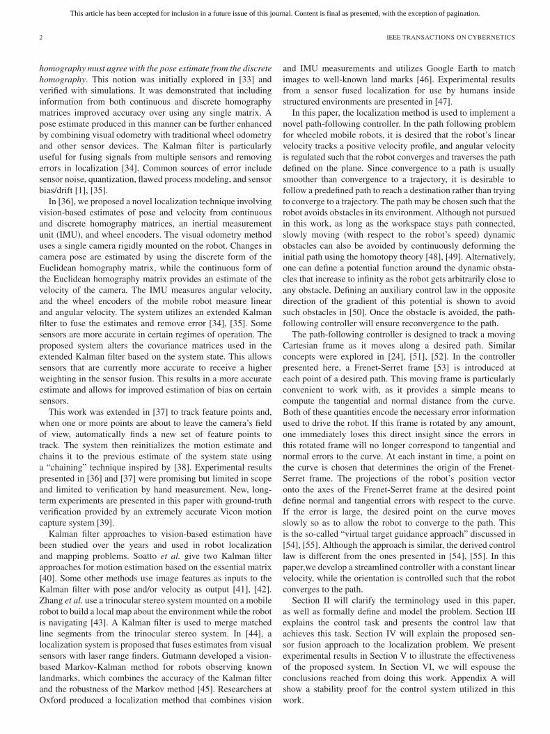
Fig. 1. Reference frames for robot and camera motion.

II. BACKGROUND

A. Robot System Overview and Formal Terminology

We employ navigation sensors that make measurements withrespect to a moving body frame. Specifically, we consider acamera body frame Fc. Sensor measurements are then rotatedto obtain localization with respect to the world frame Fw. Thepose of Fc at discrete times in the interval [t0, t1, . . . , tk−1, tk]is described in terms of a translation vector Tk ∈ R

3 and arotation matrix Rk ∈ SO(3). At any given time tk, the linearand angular velocities of the body frame Fc are described as apair of vectors vk ∈ R

3 and ωk ∈ R3.

In this paper, a camera is rigidly attached to a wheeled mo-bile robot with robot body frame Fr. The Cartesian referenceframe of the camera, Fc, is oriented such that the z-axis isoriented along the optical axis. The x-axis is oriented along thehorizontal direction of the image plane. The y-axis is orientedparallel to the vertical direction of the image. This is illustratedin Fig. 1(a). The reference frame of the robot, Fr, is attachedto the robot’s center of rotation, with x-axis aligned along therobot’s heading, y-axis oriented to the left of the robot alongthe horizontal direction, and z-axis oriented upwards along thevertical direction. Fr(tk) denotes the pose of Fr at time tk. Thisis shown in Fig. 1(a).

The origin of Fc and Fr are the same. The z-axis of Fc iscoincident with the z-axis of Fr, and the positive x-axis of Fc isthe same as the negative y-axis of Fr. Thus, they are separatedby a constant rotation Rbr.1 An IMU is rigidly attached tothe robot, with its axes aligned with Fr. Only rotations aremeasured by the IMU in this work. In this paper, the staticworld frame Fw is defined as the initial pose of the robot, i.e.,Fw = Fr(t0).

The wheeled robot is modeled as a kinematic unicycle [56]and moves in a plane spanning the x and y axes of Fw and Fr.It has two degrees of freedom. It can rotate about the z-axis ofFr with an angular velocity ωz and translate along the x-axiswith a linear velocity vx oriented along the x-axis of Fr. Thelocation of the robot in Fw at time tk is the origin of Fr(tk),given by [xr, yr, 0]

T . The orientation of the robot is θk and ismeasured by the angle between the x-axes of Fw and Fr. This

1The choice of axes orientation for Fc and Fr with respect to the cameraand robot preserves conventions of the vision and robotics communities andnaturally orients video output for humans observers. Any other constant choiceof axes can be made without loss of generality.

is illustrated in Fig. 1(b). The kinematics of the mobile robotare described by

xr = v cos(θr) (1a)

yr = v sin(θr) (1b)

θr =ω. (1c)

B. Wheel Encoders and IMU

Wheel encoders are used to measure the angular velocity ofeach wheel. The angular velocities of the left and right wheelsare given by ωL and ωR, respectively, as shown in Fig. 1(b).These measurements are converted into linear velocity of thewheels by

vL =ωL × r

vR =ωR × r

where r ∈ R+ is the constant radius of the wheels. Denoting

the constant distance between the wheels as b ∈ R+, the linear

and angular velocity of the robot is given by

vx =vL + vR

2(2a)

ωz =vL − vR

b. (2b)

The IMU measures linear acceleration using accelerometersand measures angular velocities using gyroscopes. All IMUmeasurements are with respect to Fr. Due to the constrainedmotion of the robot, we use only one of the gyros to measureangular velocity ωz .

C. Pinhole Camera Model

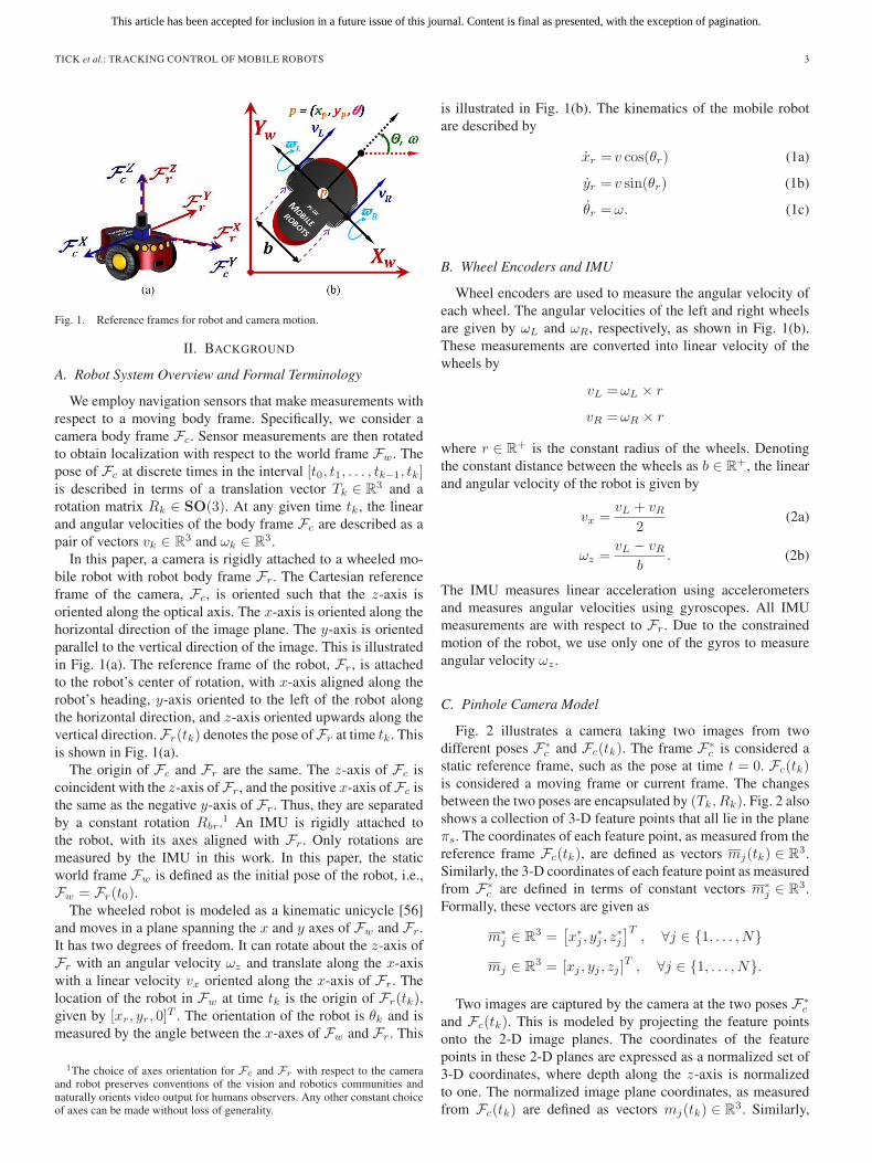
Fig. 2 illustrates a camera taking two images from twodifferent poses F∗

c and Fc(tk). The frame F∗c is considered a

static reference frame, such as the pose at time t = 0. Fc(tk)is considered a moving frame or current frame. The changesbetween the two poses are encapsulated by (Tk, Rk). Fig. 2 alsoshows a collection of 3-D feature points that all lie in the planeπs. The coordinates of each feature point, as measured from thereference frame Fc(tk), are defined as vectors mj(tk) ∈ R

3.Similarly, the 3-D coordinates of each feature point as measuredfrom F∗

c are defined in terms of constant vectors m∗j ∈ R

3.Formally, these vectors are given as

m∗j ∈ R

3 =[x∗j , y

∗j , z

∗j

]T, ∀j ∈ {1, . . . , N}

mj ∈ R3 = [xj , yj , zj ]

T , ∀j ∈ {1, . . . , N}.

Two images are captured by the camera at the two poses F∗c

and Fc(tk). This is modeled by projecting the feature pointsonto the 2-D image planes. The coordinates of the featurepoints in these 2-D planes are expressed as a normalized set of3-D coordinates, where depth along the z-axis is normalizedto one. The normalized image plane coordinates, as measuredfrom Fc(tk) are defined as vectors mj(tk) ∈ R

3. Similarly,



Fig. 2. Translation and rotation of camera frame Fc in planar scenes.

the normalized image plane coordinates of each feature pointmeasured from F∗

c are vectors m∗j ∈ R

3. These vectors areexpressed as

m∗j ∈R

3=[u∗j , v

∗j , 1

]T=[x∗j/z

∗j , y

∗j/z

∗j , 1

]T,∀j∈{1, . . . , N}

mj ∈R3=[uj , vj , 1]

T =[xj/zj , yj/zj , 1]T , ∀j∈{1, . . . , N}.

Issues of camera calibration are well understood [57], and allimage data in this work are calibrated to remove lens distortionand map points from pixel coordinates to normalized imagecoordinates.

D. Discrete and Continuous Euclidean Homography

In this paper, a visual odometry method is developed from thediscrete and continuous Euclidean homography matrices. Thisgives a vision-based estimate of position, orientation, as well aslinear and angular velocities. While the discrete homographyhas been used extensively, the continuous homography seemsto attract less attention.

Development using both Euclidean homography cases as-sumes all feature points are coplanar.2 Consider two images ofpoints mj(tk) on a plane πs. The transformation between thetwo sets of points is given by [10], [12]

mj = Rm∗j + T. (3)

The relationship in (3) can be rewritten in terms of imagepoints as

mj =

(R+

1

d∗Tn∗T

)m∗

j

2Methods to move beyond the assumption of coplanar points include virtualparallax [28] or using continuous and discrete essential matrices.

where n∗ ∈ R3 is the constant unit normal vector of plane πs

measured in F∗c , and d∗ ∈ R

+ is the constant scalar distancefrom the optical center of the camera (i.e., the origin of F∗

c ) tothe plane πs [10]. We assume that d∗ is known for the develop-ment of this section. We include a discussion of estimating d∗

in Section IV-B, in the case that d∗ is unknown.The matrix

Hd = R+1

d∗Tn∗T (4)

is the well-known Euclidean homography matrix, which wewill refer to as the discrete homography matrix. Given four ormore set of points, the matrix Hd(tk) can be recovered and usedto estimate the translation vector Tk and the rotation matrixRk [10].

In the continuous case, image point mj(tk) and its opticalflow mj(tk) are measured rather than the image pair m∗

j andmj(tk). The time derivative of mj(tk) satisfies

˙mj = ωmj + v (5)

where ω ∈ R3×3 is the skew-symmetric matrix of ω. The

relationship in (5) can be rewritten in terms of image pointsas [12]

mj =

(ω +

1

d∗vn∗T

)mj −

zjzj

.

The matrix

Hc = ω +1

d∗vn∗T

is defined as the continuous homography matrix. Similar tothe discrete form, an algorithm exists to solve for Hc(tk) andestimate the linear velocity vk and angular velocity ωk [12].

III. ROBOT CONTROL SYSTEM

We provide a control algorithm to guide a unicycle robot,whose differential kinematic model is given by (1), to followa parametrized path, γ : [0, smax] � s �→ γ(s) ∈ R

2. In thisdevelopment, the robot’s configuration space M is taken asthe quotient space M = (R2 × R/2kπ, k ∈ Z) � R

2 × S1 �SE(2). The Frenet-Serret frame of a curve is a set of n-orthonormal vectors that are naturally fitted at every point onthe curve [53]. On a 3-D Euclidean space, the three orthonor-mal vectors {e1, e2, e3} are conveniently defined using theGram-Schmidt orthonormalization process [58]

e1(s) =γ′(s)

‖γ′(s)‖ (6a)

e2(s) =γ′′(s)−〈γ′′(s), e1(s)〉 e1(s)

‖γ′′(s)−〈γ′′(s), e1(s)〉 e1(s)‖(6b)

e3(s) =γ′′′(s)−〈γ′′′(s), e1(s)〉 e1(s)−〈γ′′′(s), e2s)〉 e2(s)

‖γ′′′(s)−〈γ′′′(s), e1(s)〉 e1(s)−〈γ′′′(s), e2s)〉 e2(s)‖(6c)



Fig. 3. World, robot and Frenet-Serret frames.

where 〈·, ·〉 denotes the standard inner product on R3, and ‖ · ‖

denotes the 2-norm on R3. One of the most important intrinsic

constants of a curve is its curvature, given by

κ(s) =〈e′1(s), e2(s)〉

‖γ′(s)‖ . (7)

Define the coordinates of the map γ by (xf , yf ). Similarly,the orthonormal vectors {e1, e2, e3}, define the orientation ofthe embedded submanifold (curve) [49]. A parametrization ofthe orientation θf can be taken as

θf (s) = arctan〈e1(s), yw〉〈e1(s), xw〉

(8)

where [xw, yw]T are the x and y components of the world

frame.It is more convenient to work with local coordinates by

expressing the equations of motion in the Frenet-Serret frame.To this end, define the variables [x1, x2, x3]

T

[x1

x2

]=RT

[xr − xf

yr − yf

](9a)

x3 = θr − θf (9b)

where R ∈ SO(2) encodes the orientation of the Frenet-Serretframe with respect to the inertial frame; i.e., rotation in theplane by θf . While [x1, x2]

T denotes the position vector fromthe origin of the Frenet-Serret frame to the origin of the robot,x3 gives the orientation of the robot with respect to the Frenet-Serret frame. As illustrated in Fig. 3, we identify [x1, x2]

T asthe components of the vector pfr emanating from the origin ofthe Frenet-Serret frame and ending at the origin of the robot.

To find the equations of motion governing the evolution ofthe robot pose with respect to the Frenet-Serret frame, we mustfirst express pfr in the world frame as

pr = γ +Rpfr (10a)

pfr =RT (pr − γ). (10b)

Differentiating (10) with respect to time and noting that γ is notparametrized by time, but by a function of time s(t), gives

pfr = RT (pr − γ) +RT

(pr −

dγ

dss

). (11)

Combining (1) and (7)–(11) gives the differential equations

x1 = v cosx3 − (1− κx2)s (12a)

x2 = v sinx3 − κx1s (12b)

x3 = − ω − κs. (12c)

We now define what is meant by convergence to the curve.If [xr0, yr0, θr0]

T is an initial condition for the differentialequations (1), a control law u = [u1, u2, u3]

T = [v, ω, s]T isconvergent to the curve γ if

limt→∞

[xr, yr, θr]T = [xf , yf , θf ]

T . (13)

To provide a streamlined controller, we place a constant forwardvelocity constraint and set u1 = u10 > 0 a constant.

Theorem 1: The system of differential equations (12), gov-erning the evolution of the robot pose with respect to the Frenet-Serret frame, is globally asymptotically stable to the origin (i.e.,(13) holds), with the state feedback given by

u1 =u10 (14a)

u2 =x2 − u10κ cos(x3) + λ2u10 sin(x3)− λ3κx1 (14b)

u3 =u10 cos(x3) + λ3x1 (14c)

where the positive control gains λ1, λ2 > 0 and the mobilerobot linear velocity u10 > 0 satisfy λ3/λ2 ≤ u10.

Proof: The proof of this theorem is found in Appendix A.

IV. POSE ESTIMATION SYSTEM

We propose a system for localization and control of a mobilerobot via fusion of vision-based pose and velocity estimateswith velocity estimates from an IMU and wheel odometry. Anextended Kalman filter is used to perform the sensor fusion andincorporate the known kinematics of the system to reduce theeffects of sensor noise and bias.

A. Robot Pose and Velocity Estimation

The system is described by the discrete state space equations

xk =Fk · xk−1 + qk (15a)

yk =Hk · xk + rk. (15b)

In (15a) and (15b), xk is the state vector, Fk is the statetransition matrix, yk is the measurement vector, Hk is themeasurement matrix, and qk and rk are normally distributedrandom processes with zero mean and covariance matrices Qk

and Rk, respectively.Localization of a kinematic unicycle mobile robot requires

knowledge of the robot position xr(tk) and yr(tk) and rotationθ(tk), all measured in the world frame Fw. Robot velocityvx(tk) and angular velocity ωz(tk) are included in the state,as measured in the robot frame. One drawback of IMUs is thatthey suffer a bias on the angular velocity measurements. Thisbias will be integrated over time and produce a large drift errorin the orientation estimate. This problem is particularly notable



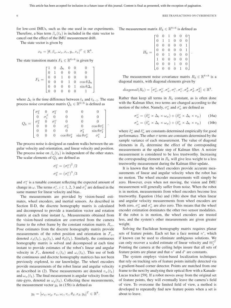
for low-cost IMUs, such as the one used in our experiments.Therefore, a bias term βω(tk) is included in the state vector tocancel out the effect of the IMU measurement drift.

The state vector is given by

xk = [θ, βω, ωz, xr, yr, vx]T ∈ R

6.

The state transition matrix Fk ∈ R6×6 is given by

Fk =

⎡⎢⎢⎢⎢⎢⎣

1 0 Δt 0 0 00 1 0 0 0 00 0 1 0 0 00 0 0 1 0 cos θΔt

0 0 0 0 1 sin θΔt

0 0 0 0 0 1

⎤⎥⎥⎥⎥⎥⎦

where Δt is the time difference between tk and tk−1. The stateprocess noise covariance matrix Qk ∈ R

6×6 is defined as

Qk =

⎡⎢⎢⎢⎢⎢⎢⎣

σω3 0 σω

2 0 0 0

0 σβ1 0 0 0 0

σω2 0 σω

1 0 0 00 0 0 σv

3 0 cos θσv2

0 0 0 0 σv3 sin θσv

2

0 0 0 cos θσv2 sin θσv

2 σv1

⎤⎥⎥⎥⎥⎥⎥⎦.

The process noise is designed as random walks between the an-gular velocity and orientation, and linear velocity and position.The process noise on βω(tk) is independent of the other states.The scalar elements of Qk are defined as

σω2 = (σω

1 )2 /2

σω3 = (σω

1 )3 /3

and σω1 is a tunable constant reflecting the expected amount of

change in ω. The terms σvi , i ∈ 1, 2, 3 and σβ

1 are defined in thesame manner for linear velocity and bias.

The measurements are provided by vision-based esti-mates, wheel encoders, and inertial sensors. As described inSection II-D, the discrete homography matrix is calculatedand decomposed to provide a translation vector and rotationmatrix at each time instant tk. Measurements obtained fromthe vision-based estimation are converted from the cameraframe to the robot frame by the constant rotation matrix Rcr.Pose estimates from the discrete homography matrix providemeasurements of the robot position and orientation in Fw,denoted xd(tk), yd(tk), and θd(tk). Similarly, the continuoushomography matrix is solved and decomposed at each timeinstant to provide estimates of the robot’s linear and angularvelocity in Fr, denoted vc(tk) and ωc(tk). This use of boththe continuous and discrete homography matrices has not beenpreviously explored, to our knowledge. The wheel encodersprovide measurements of the robot linear and angular velocityas described in (2). These measurements are denoted vw(tk)and ωw(tk). The final measurement is angular velocity from therate-gyro, denoted as ωg(tk). Collecting these measurements,the measurement vector yk in (15b) is defined as

yk = [ωw, ωg, vw, ωc, vc, θd, xd, yd]T ∈ R

8.

The measurement matrix Hk ∈ R8×6 is defined as

Hk =

⎡⎢⎢⎢⎢⎢⎢⎢⎢⎢⎣

0 0 1 0 0 00 1 1 0 0 00 0 0 0 0 10 0 0 0 0 10 0 1 0 0 01 0 0 0 0 00 0 0 1 0 00 0 0 0 1 0

⎤⎥⎥⎥⎥⎥⎥⎥⎥⎥⎦.

The measurement noise covariance matrix Rk ∈ R8×8 is a

diagonal matrix, with diagonal elements given by

diagonal(Rk) =[σωw, σ

ωg , σ

vw, σ

ωc , σ

ωv , σ

θd, σ

xd , σ

yd

]∈ R

8.

Rather than keep all terms in Rk constant, as is often donewith the Kalman filter, two terms are changed according to themotion of the robot. Namely, σω

w and σvw are defined as

σωw = (δωw ×Δt × ωw) + (δωw ×Δt × vw) (16a)

σvw = (δvw ×Δt × ωw) + (δvw ×Δt × vw) (16b)

where δωw and δvw are constants determined empirically for goodperformance. The other σ terms are constants determined by thesample variance of each measurement. The value of diagonalelements in Rk determine the effect of the correspondingmeasurements at the update step of Kalman filter. A noisiermeasurement is considered to be less trustworthy. Increasingthe corresponding element in Rk will give less weight to a lesstrustworthy measurement during the Kalman filter update.

It is known that the wheel encoders provide accurate mea-surements of linear and angular velocity when the robot hasno motion. The wheel encoder measurements will simply bezero. However, even when not moving, the vision and IMUmeasurement will generally suffer from noise. When the robotis in motion, measurements from wheel encoders become lesstrustworthy. Equation (16a) and (16b) show that when linearand angular velocity measurements from wheel encoders areboth zero, σω

w and σvw are also zero. This means that the wheel

encoder estimation dominates the other two sensor modalities.If the robot is in motion, the wheel encoders are trustedless, and the system’s other measurements are given greaterweight.

Solving the Euclidean homography matrix requires planarsets of feature points. Each set has a face normal n∗, whichif known can be used to eliminate ambiguous solutions. Wecan only recover a scaled estimate of linear velocity and m∗T

j

Pointing the camera at the ceiling helps insure that all sets offeature points are planar and that n∗ and d∗ are constants.

The system employs vision-based localization techniquesthat rely on tracking sets of feature points initially detected viaa gradient-based corner detector. Points are matched from oneframe to the next by analyzing their optical flow with a Kanade-Lucas tracker [59]. If a robot moves away from the original setof feature points, they will eventually leave the camera’s fieldof view. To overcome the limited field of view, a method isdeveloped to repeatedly find new feature points when a set isabout to leave.



Fig. 4. Annotated camera view.

Each captured image is divided into three regions of interest(ROIs) as shown in Fig. 4. The two green boxes represent theROI borders, while the arrows and numbers added to Fig. 4denote the number of pixels that separate each of the ROIs. Allfeature points to be tracked (labeled for the reader) are initiallylocated within the inner ROI. If the corner tracker detects thatone or more feature points have left the outer ROI, it searchesfor a new set of feature points that all lie within the inner ROI(not necessarily mutually exclusive with respect to the old set).It continues to track the old points until the new features arefound. At this point, the system starts tracking the new points,resets the position and orientation estimate measured by thediscrete homography matrix to zero, and “chains” it to thesystem’s current state.

Consider a set of points tracked starting at time tj . Therotation and translation Rj and Tj give the robot’s pose inthe world frame at time tj . Over the time period [tj , . . . , tk],the change in pose is measured by the discrete homographymatrix and is given by Rk

j and T kj in the camera frame at time

tj . The current pose in the world frame is given by

Rk =Rj

(Rk

j

)T(17a)

Tk = −Rj

(Rk

j

)TT kj + Tj . (17b)

When a chaining event occurs, Rj and Tj are updated to themost recent value given by (17a) and (17b).

With the chaining of estimates from the homography matrix,vision data can be a reliable source for localizing mobile robots.However, estimation from homography can be inaccurate orunavailable in some cases. Tracked feature points tend to driftas the camera moves if they are not associated with a strongenough local gradient in the image. This condition is detectedby monitoring the tracking error for each point between timesteps. Most feature point detection algorithms include a mea-sure of feature quality. For example, the quality of a cornerfeatures is defined by the magnitude of the local gradient intwo directions. In some cases, insufficient features with highquality can be found within the inner ROI. In these situations,the system temporarily switches over to a reduced systemcomprised of only IMU and wheel encoder measurements. The

relevant information from the system’s EKF is copied into thereduced system’s EKF. When the vision system detects enoughgood features again, the reduced system is halted and relevantinformation is then copied back into the system’s full EKF.

The reduced system does not have any vision measurements.Since it does not have the XY position or orientation estimatesfrom the discrete homography matrix, the reduced system maybe more susceptible to drift, as it is well known that estimatorsbased only on velocity are generally not observable. However,when the full system is in operation, all components of thestate vector are directly measured, and pose estimates arereinstated.

In [37], it is shown in experiments that the trace of the errorcovariance matrix for the full system typically converges to aconstant limit, although the trajectory is noisy. This suggeststhat the Kalman gain will remain bounded as well. Further-more, this indicates that the estimation error that builds up inthe system over time is bounded. This is made possible byincluding direct measurements of θk, xrk, and yrk from thediscrete homography matrix. Without these measurements, theestimation error would likely be unbounded.

B. Depth Estimation

If the depth term d∗ is not known, it can be estimated[60], [61]. We present a Kalman filter-based depth estima-tion method. The depth estimation can be ran as a separate,1-D Kalman filter, or appended to the EKF described inSection IV-A.

From the definition of the discrete homography matrix in(4), we have Td = T/d∗ as the scaled translation returned bysolving the discrete homography. Given the measurement Td, ifTd �= 0 and T is known, d∗ can be solved as

d∗ =TTd T

TTd Td

=TTd T

‖Td‖2. (18)

We denote the estimate of d∗ at time k as d∗k. The differenceequation of the depth estimate is

d∗k+1 = d∗k + qdk (19)

where qdk is a scalar, normal random variable with zero mean.This reflects an assumption that the depth is constant or slowlyvarying, which is a reasonable assumption for indoor environ-ments. We use a variation of (18) as a measurement of d∗

ydk =TTdkTk

‖Tdk‖2(20)

where Tk is the estimate of the translation at time k, and Tdk isthe scaled translation measurement recovered from the discretehomography. We assume a zero-mean, white noise term isadded to the measurement (20), denoted rdk.

Equations (19) and (20), along with the variance of qdk andrdk, are sufficient to run the prediction and update equationsof a 1-D depth estimation Kalman filter. Alternately, dk can beincluded in the EKF described in Section IV-A. This requiresthat dk be appended to xk and ydk appended to yk. Appropriate



rows and columns must be added to Fk, Hk, Qk, and Rk. Asdescribed in (19) and (20), the new state and measurement aretreated as independent of the other states and measurements, soadditional rows and columns will be zero except for one ele-ment corresponding to the new state. The number of operationsfor a Kalman filter increases quadratically with the number ofvariables in the state, but seven states is still relatively small.

There are several issues that should be noted when includingthe depth estimation in the proposed system. First, at startup,d∗ is unknown and the translation solution from the discretehomography cannot be properly scaled for use in the EKF.Until d∗ has converged, the elements of Rk, σx

d , and σyd are

kept large (an order of magnitude larger than typical). Thisinduces the update step to largely ignore this measurementuntil d∗ is trusted. Second, Tdk is measured from the start ofthe previous chaining event. Therefore, Tk in (20) should alsobe the estimated translation since the last chaining event, notsince system start. Finally, care must be taken when Tdk = 0at system startup or after a chaining event. Sensor noise willusually prevent this, but if Tdk = 0, it should be replaced witha small constant in (20) to prevent singularity.

V. EXPERIMENTAL RESULTS

Extensive experiments have been carried out to demonstratethe effectiveness of the proposed control and pose estimationmethods. The experiments presented in this paper are measuredthroughout their entire duration with a Vicon MX MotionCapture System [39]. The Vicon system is comprised of anarray of eight Vicon T-20S infrared motion capture camerasmounted on the wall around the lab. A set of spherical infraredmarkers are affixed to the deck of the robot. Based on thecamera views of the infrared markers, the Vicon system canestimate the position and orientation of the robot with sub-millimeter accuracy at a capture rate of approximately 100Hz.This provides a reliable ground truth to compare our system’sperformance.

The robot used in these experiments is a Pioneer 3-DX two-wheel differential drive robot. The IMU is a Nintendo WiiRemote (Wiimote) with MotionPlus. This IMU costs approxi-mately $42 US dollars and represents a very low-cost option foran IMU. The camera used is a matrix Vision BlueFox camera.The camera is mounted on the robot such that the center of thecamera is aligned with the robot’s center of rotation, and thecamera axes are aligned with robot axes as closely as possible.An example image captured from the camera during system op-eration is shown in Fig. 4. Much of the image processing in thisdevelopment utilizes the OpenCV library [62]. A Dell M6400mobile workstation with an Intel Core Duo processor is affixedto the robot and collects all measurements and performs imageprocessing, vision algorithms, path planning, robot control, userI/O, communication of high-level commands to the robot, aswell as operating the extended Kalman filter.

A. Localization and Control Using Known Depth

A simple GUI-based path planning module has been in-tegrated into the system (see Fig. 5). The user is presented

Fig. 5. Cropped screen shot of the plan Planning GUI with legend on bottom.Scale map of the SeRViCE (right side) and LARS (left side) labs at UTD. Thegrayish colored grid lines are one meter by one meter. Walls are shown as thickorange lines. Pink areas are forbidden regions which contain obstacle or otherhazards that the robot should avoid. The green boxes demarcate the locationsof possible points of interest that the robot may want to visit. The robot’scurrent position and orientation are marked with a white triangle. The way-points selected by the user are shown as little yellow dots and are connected toeach other in order with a series of blue line segments. The interpolated splinecurve generated by Sintef Spline Library to connect all of the way-points inorder is plotted in red. The cyan dot represents the current desired position ofthe robot. As the robot chases the dot, its path is drawn as a magenta line.

with a scale map of the Sensing, Robotics, Vision, Control,and Estimation (SeRViCE) Lab and the adjoining Laboratoryfor Autonomous Robotic Systems (LARS) at the Universityof Texas at Dallas. Walls and potential points of interest aremarked on the map. In addition, the map demarcates “forbid-den” regions that contain obstacles or hazards that the robotmust avoid.

The robot’s current position and orientation are marked witha white triangle. First, the user decides where they want to sendthe robot by selecting a series of way-points for the robot tovisit in order. When finished plotting all of the way-points, aNon-Uniform Rational Bezier-Spline (NURBS) curve is fittedto the selected points using the Sintef Spline Library (SISL)[63]. A colored dot will appear on or near the beginning of thecurve. This dot represents the current desired position of therobot. Formally speaking, the cyan dot represents the point son the curve γ (red line in Fig. 5) as described previously inSection III. The estimation and control algorithms detailed inthis paper enable the robot to follow the desired path along theBezier curve to reach all desired way-points.

The formal experiments presented in this paper all utilizethis path planning system with a set of preloaded points on aLissajous curve. The Lissajous curve is chosen as a path be-cause it requires the robot to turn equal amounts both clockwiseand counter clockwise in a single circuit. It also causes the robotto have to constant change its angular velocity in order to stayon the curve. In addition, the robot’s orientation will eventuallycycle through all values in the interval [0, 2π], and the robot’sposition should pass through all x-axis values in the interval[−Ax, Ax] as well as all y-axis values in the interval [−Ay, Ay]in a periodic fashion.



Fig. 6. Plot of parametric form Lissajous curve showing the asymptotic pointsgiven as input to the path planner.

Fig. 7. X-position, Y-position, and orientation experiment #7.

Fig. 6 shows a plot of a Lissajous curve and its sevenasymptotic points where either xt = (−Ax, Ox, Ax) or yt =(−Ay, Oy, Ay). These seven asymptotes are given as inputto the path planner (with (Ox, Oy) given twice to make atotal of eight points), and SISL calculates a NURBS curve tointerpolate the point set. The resulting NURBS curve (shownin Fig. 6 as a dashed gray line) is then loaded as the robot’sintended path. Due to the nature of the spline interpolation,the plotted curve deviates somewhat from a Lissajous curve butretains its relevant properties.

When the experiment starts, the robot is not on the curveand must converge to it over the course of the experiment.The robot is started at coordinates [−4524 mm,−1524 mm]T ,approximately 1.5 m away along both the X and Y axes fromthe curve’s origin point [Ox, Oy]

T labeled C in Fig. 6. Therobot is told to trace the pattern three times. This experimentwas repeated eight times. As the Vicon and robot data aresampled at different rates, the Vicon data was downsampled tomatch the robot rate. The total distance traveled by the robot isapproximately 18 m.

Fig. 7 shows comparisons between the robot localizationestimate (red dotted line) and the robot’s actual position asmeasured by the Vicon (blue dashed line) for X-position,Y -position, and θ-orientation. Fig. 8 shows an XY plot of therobot data (red dots) versus the Vicon’s measurements (bluedashes) overlaid on top of the robot’s intended path (black solidline) as calculated by the path planning module. Qualitatively

Fig. 8. Path for experiment #7.

Fig. 9. Comparison of linear and angular velocity for experiment #7.

speaking, in all four data sets, the red and blue lines are almostright on top of each other during the entire experiment. Thecontrol algorithm is also verified to work well, as the robot doesnot deviate far from the desired curve.

One strength of our proposed method is that it measuresand estimates both linear and angular velocity, but the Vicononly measures position. A ground-truth velocity estimate wascreated by backwards differencing the Vicon estimates andapplying a low-pass filter. A plot of the velocities is shown inFig. 9. Note the large amount of noise present in the Vicon’slinear velocity estimate, even after the filter is applied.

On a more quantitative level, the root mean squared (RMS)error between the robot’s estimates and the Vicon’s measure-ments is calculated for X-position, Y -position, θ-orientation,as well as the L2 norm (Euclidean distance) between the XYposition estimated by the robot and the position measured bythe Vicon during each experiment. The mean and standarddeviation (STD) of the RMS error is calculated for the eight ex-periments, and this is presented in Table I. As an alternative, thetrajectory and path data for each experiment from both the robotand Vicon is averaged creating “the average path.” Figs. 10 and11 show the same information as Figs. 7 and 8, but for the“average path” instead of just a single experiment. Then, RMSerror for the average path X-position, Y -position, θ-orientation,



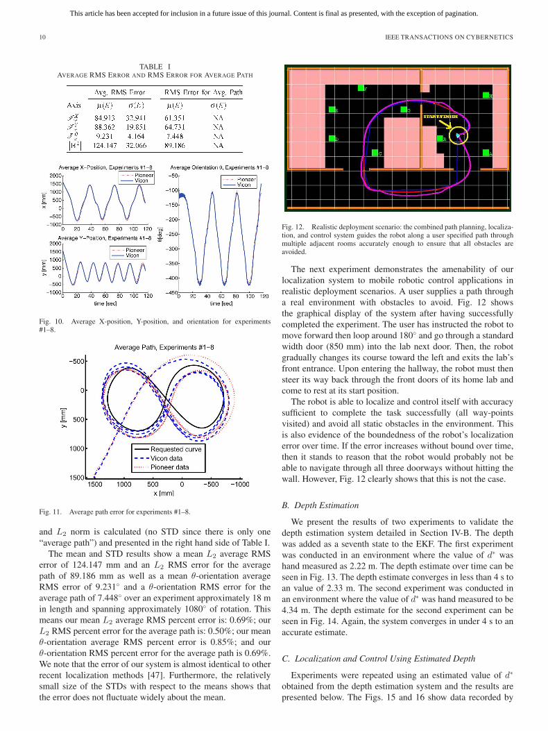
TABLE IAVERAGE RMS ERROR AND RMS ERROR FOR AVERAGE PATH

Fig. 10. Average X-position, Y-position, and orientation for experiments#1–8.

Fig. 11. Average path error for experiments #1–8.

and L2 norm is calculated (no STD since there is only one“average path”) and presented in the right hand side of Table I.

The mean and STD results show a mean L2 average RMSerror of 124.147 mm and an L2 RMS error for the averagepath of 89.186 mm as well as a mean θ-orientation averageRMS error of 9.231◦ and a θ-orientation RMS error for theaverage path of 7.448◦ over an experiment approximately 18 min length and spanning approximately 1080◦ of rotation. Thismeans our mean L2 average RMS percent error is: 0.69%; ourL2 RMS percent error for the average path is: 0.50%; our meanθ-orientation average RMS percent error is 0.85%; and ourθ-orientation RMS percent error for the average path is 0.69%.We note that the error of our system is almost identical to otherrecent localization methods [47]. Furthermore, the relativelysmall size of the STDs with respect to the means shows thatthe error does not fluctuate widely about the mean.

Fig. 12. Realistic deployment scenario: the combined path planning, localiza-tion, and control system guides the robot along a user specified path throughmultiple adjacent rooms accurately enough to ensure that all obstacles areavoided.

The next experiment demonstrates the amenability of ourlocalization system to mobile robotic control applications inrealistic deployment scenarios. A user supplies a path througha real environment with obstacles to avoid. Fig. 12 showsthe graphical display of the system after having successfullycompleted the experiment. The user has instructed the robot tomove forward then loop around 180◦ and go through a standardwidth door (850 mm) into the lab next door. Then, the robotgradually changes its course toward the left and exits the lab’sfront entrance. Upon entering the hallway, the robot must thensteer its way back through the front doors of its home lab andcome to rest at its start position.

The robot is able to localize and control itself with accuracysufficient to complete the task successfully (all way-pointsvisited) and avoid all static obstacles in the environment. Thisis also evidence of the boundedness of the robot’s localizationerror over time. If the error increases without bound over time,then it stands to reason that the robot would probably not beable to navigate through all three doorways without hitting thewall. However, Fig. 12 clearly shows that this is not the case.

B. Depth Estimation

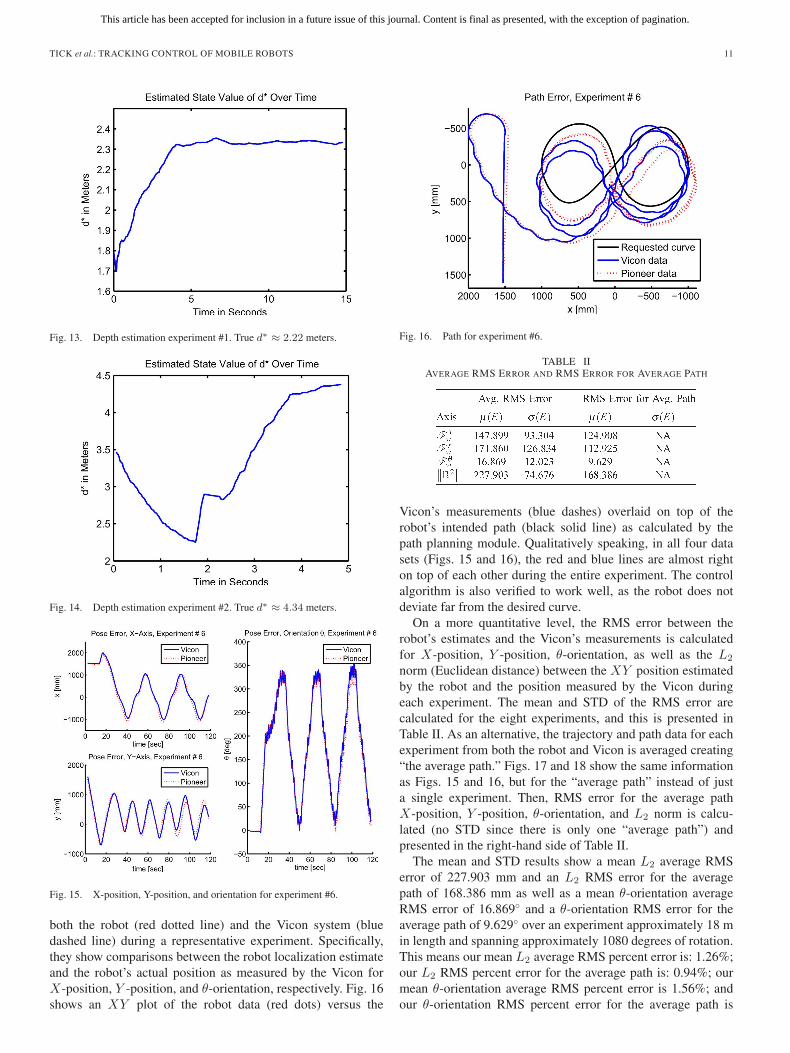
We present the results of two experiments to validate thedepth estimation system detailed in Section IV-B. The depthwas added as a seventh state to the EKF. The first experimentwas conducted in an environment where the value of d∗ washand measured as 2.22 m. The depth estimate over time can beseen in Fig. 13. The depth estimate converges in less than 4 s toan value of 2.33 m. The second experiment was conducted inan environment where the value of d∗ was hand measured to be4.34 m. The depth estimate for the second experiment can beseen in Fig. 14. Again, the system converges in under 4 s to anaccurate estimate.

C. Localization and Control Using Estimated Depth

Experiments were repeated using an estimated value of d∗

obtained from the depth estimation system and the results arepresented below. The Figs. 15 and 16 show data recorded by



Fig. 13. Depth estimation experiment #1. True d∗ ≈ 2.22 meters.

Fig. 14. Depth estimation experiment #2. True d∗ ≈ 4.34 meters.

Fig. 15. X-position, Y-position, and orientation for experiment #6.

both the robot (red dotted line) and the Vicon system (bluedashed line) during a representative experiment. Specifically,they show comparisons between the robot localization estimateand the robot’s actual position as measured by the Vicon forX-position, Y -position, and θ-orientation, respectively. Fig. 16shows an XY plot of the robot data (red dots) versus the

Fig. 16. Path for experiment #6.

TABLE IIAVERAGE RMS ERROR AND RMS ERROR FOR AVERAGE PATH

Vicon’s measurements (blue dashes) overlaid on top of therobot’s intended path (black solid line) as calculated by thepath planning module. Qualitatively speaking, in all four datasets (Figs. 15 and 16), the red and blue lines are almost righton top of each other during the entire experiment. The controlalgorithm is also verified to work well, as the robot does notdeviate far from the desired curve.

On a more quantitative level, the RMS error between therobot’s estimates and the Vicon’s measurements is calculatedfor X-position, Y -position, θ-orientation, as well as the L2

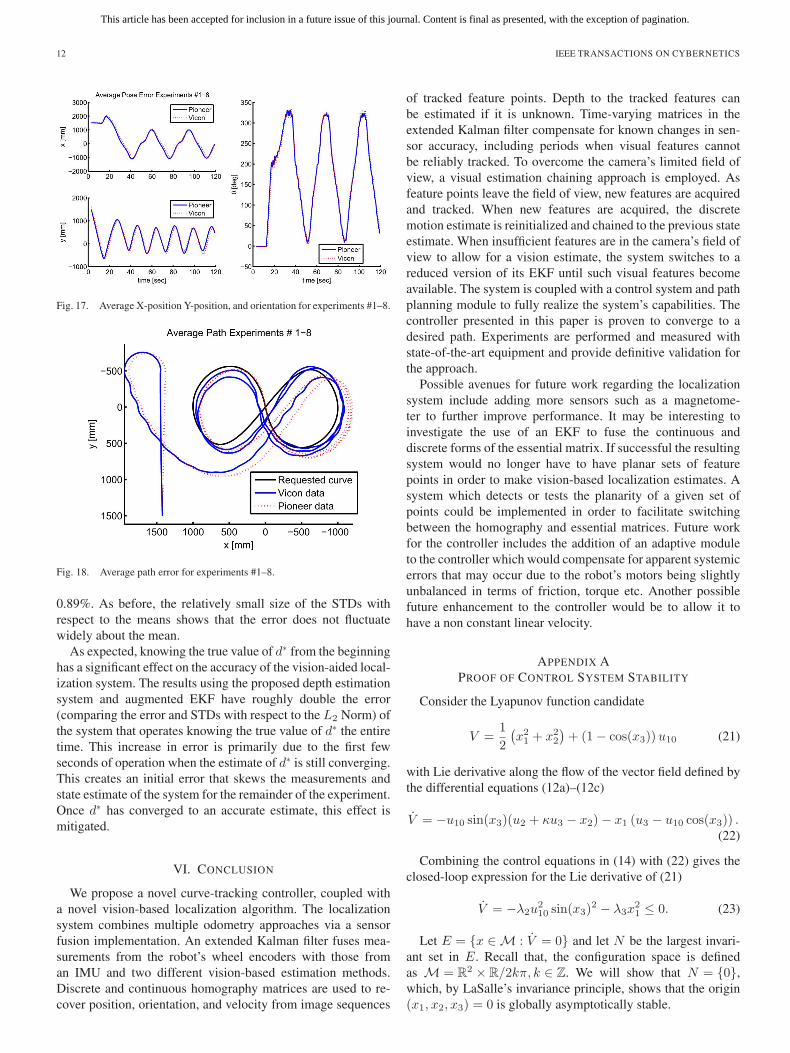
norm (Euclidean distance) between the XY position estimatedby the robot and the position measured by the Vicon duringeach experiment. The mean and STD of the RMS error arecalculated for the eight experiments, and this is presented inTable II. As an alternative, the trajectory and path data for eachexperiment from both the robot and Vicon is averaged creating“the average path.” Figs. 17 and 18 show the same informationas Figs. 15 and 16, but for the “average path” instead of justa single experiment. Then, RMS error for the average pathX-position, Y -position, θ-orientation, and L2 norm is calcu-lated (no STD since there is only one “average path”) andpresented in the right-hand side of Table II.

The mean and STD results show a mean L2 average RMSerror of 227.903 mm and an L2 RMS error for the averagepath of 168.386 mm as well as a mean θ-orientation averageRMS error of 16.869◦ and a θ-orientation RMS error for theaverage path of 9.629◦ over an experiment approximately 18 min length and spanning approximately 1080 degrees of rotation.This means our mean L2 average RMS percent error is: 1.26%;our L2 RMS percent error for the average path is: 0.94%; ourmean θ-orientation average RMS percent error is 1.56%; andour θ-orientation RMS percent error for the average path is



Fig. 17. Average X-position Y-position, and orientation for experiments #1–8.

Fig. 18. Average path error for experiments #1–8.

0.89%. As before, the relatively small size of the STDs withrespect to the means shows that the error does not fluctuatewidely about the mean.

As expected, knowing the true value of d∗ from the beginninghas a significant effect on the accuracy of the vision-aided local-ization system. The results using the proposed depth estimationsystem and augmented EKF have roughly double the error(comparing the error and STDs with respect to the L2 Norm) ofthe system that operates knowing the true value of d∗ the entiretime. This increase in error is primarily due to the first fewseconds of operation when the estimate of d∗ is still converging.This creates an initial error that skews the measurements andstate estimate of the system for the remainder of the experiment.Once d∗ has converged to an accurate estimate, this effect ismitigated.

VI. CONCLUSION

We propose a novel curve-tracking controller, coupled witha novel vision-based localization algorithm. The localizationsystem combines multiple odometry approaches via a sensorfusion implementation. An extended Kalman filter fuses mea-surements from the robot’s wheel encoders with those froman IMU and two different vision-based estimation methods.Discrete and continuous homography matrices are used to re-cover position, orientation, and velocity from image sequences

of tracked feature points. Depth to the tracked features canbe estimated if it is unknown. Time-varying matrices in theextended Kalman filter compensate for known changes in sen-sor accuracy, including periods when visual features cannotbe reliably tracked. To overcome the camera’s limited field ofview, a visual estimation chaining approach is employed. Asfeature points leave the field of view, new features are acquiredand tracked. When new features are acquired, the discretemotion estimate is reinitialized and chained to the previous stateestimate. When insufficient features are in the camera’s field ofview to allow for a vision estimate, the system switches to areduced version of its EKF until such visual features becomeavailable. The system is coupled with a control system and pathplanning module to fully realize the system’s capabilities. Thecontroller presented in this paper is proven to converge to adesired path. Experiments are performed and measured withstate-of-the-art equipment and provide definitive validation forthe approach.

Possible avenues for future work regarding the localizationsystem include adding more sensors such as a magnetome-ter to further improve performance. It may be interesting toinvestigate the use of an EKF to fuse the continuous anddiscrete forms of the essential matrix. If successful the resultingsystem would no longer have to have planar sets of featurepoints in order to make vision-based localization estimates. Asystem which detects or tests the planarity of a given set ofpoints could be implemented in order to facilitate switchingbetween the homography and essential matrices. Future workfor the controller includes the addition of an adaptive moduleto the controller which would compensate for apparent systemicerrors that may occur due to the robot’s motors being slightlyunbalanced in terms of friction, torque etc. Another possiblefuture enhancement to the controller would be to allow it tohave a non constant linear velocity.

APPENDIX APROOF OF CONTROL SYSTEM STABILITY

Consider the Lyapunov function candidate

V =1

2

(x21 + x2

2

)+ (1− cos(x3))u10 (21)

with Lie derivative along the flow of the vector field defined bythe differential equations (12a)–(12c)

V = −u10 sin(x3)(u2 + κu3 − x2)− x1 (u3 − u10 cos(x3)) .(22)

Combining the control equations in (14) with (22) gives theclosed-loop expression for the Lie derivative of (21)

V = −λ2u210 sin(x3)

2 − λ3x21 ≤ 0. (23)

Let E = {x ∈ M : V = 0} and let N be the largest invari-ant set in E. Recall that, the configuration space is definedas M = R

2 × R/2kπ, k ∈ Z. We will show that N = {0},which, by LaSalle’s invariance principle, shows that the origin(x1, x2, x3) = 0 is globally asymptotically stable.



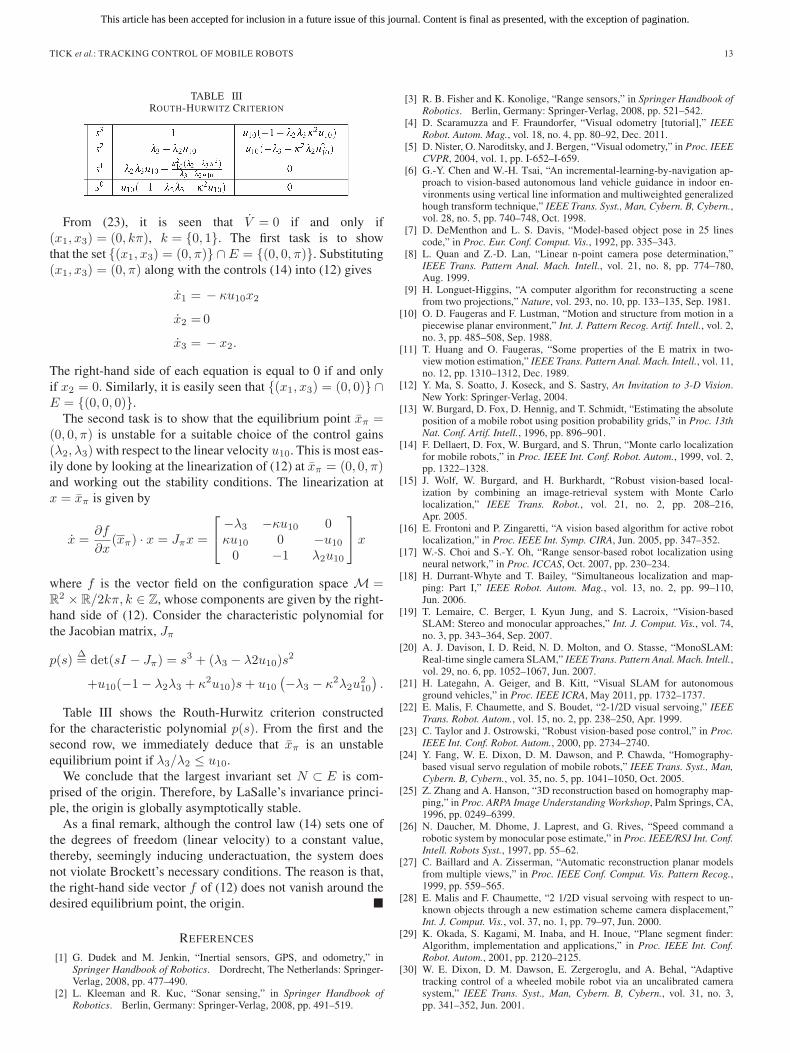
TABLE IIIROUTH-HURWITZ CRITERION

From (23), it is seen that V = 0 if and only if(x1, x3) = (0, kπ), k = {0, 1}. The first task is to showthat the set {(x1, x3) = (0, π)} ∩ E = {(0, 0, π)}. Substituting(x1, x3) = (0, π) along with the controls (14) into (12) gives

x1 = − κu10x2

x2 =0

x3 = − x2.

The right-hand side of each equation is equal to 0 if and onlyif x2 = 0. Similarly, it is easily seen that {(x1, x3) = (0, 0)} ∩E = {(0, 0, 0)}.

The second task is to show that the equilibrium point xπ =(0, 0, π) is unstable for a suitable choice of the control gains(λ2, λ3) with respect to the linear velocity u10. This is most eas-ily done by looking at the linearization of (12) at xπ = (0, 0, π)and working out the stability conditions. The linearization atx = xπ is given by

x =∂f

∂x(xπ) · x = Jπx =

⎡⎣ −λ3 −κu10 0κu10 0 −u10

0 −1 λ2u10

⎤⎦x

where f is the vector field on the configuration space M =R

2 × R/2kπ, k ∈ Z, whose components are given by the right-hand side of (12). Consider the characteristic polynomial forthe Jacobian matrix, Jπ

p(s)Δ= det(sI − Jπ) = s3 + (λ3 − λ2u10)s

2

+u10(−1− λ2λ3 + κ2u10)s+ u10

(−λ3 − κ2λ2u

210

).

Table III shows the Routh-Hurwitz criterion constructedfor the characteristic polynomial p(s). From the first and thesecond row, we immediately deduce that xπ is an unstableequilibrium point if λ3/λ2 ≤ u10.

We conclude that the largest invariant set N ⊂ E is com-prised of the origin. Therefore, by LaSalle’s invariance princi-ple, the origin is globally asymptotically stable.

As a final remark, although the control law (14) sets one ofthe degrees of freedom (linear velocity) to a constant value,thereby, seemingly inducing underactuation, the system doesnot violate Brockett’s necessary conditions. The reason is that,the right-hand side vector f of (12) does not vanish around thedesired equilibrium point, the origin. �

REFERENCES

[1] G. Dudek and M. Jenkin, “Inertial sensors, GPS, and odometry,” inSpringer Handbook of Robotics. Dordrecht, The Netherlands: Springer-Verlag, 2008, pp. 477–490.

[2] L. Kleeman and R. Kuc, “Sonar sensing,” in Springer Handbook ofRobotics. Berlin, Germany: Springer-Verlag, 2008, pp. 491–519.

[3] R. B. Fisher and K. Konolige, “Range sensors,” in Springer Handbook ofRobotics. Berlin, Germany: Springer-Verlag, 2008, pp. 521–542.

[4] D. Scaramuzza and F. Fraundorfer, “Visual odometry [tutorial],” IEEERobot. Autom. Mag., vol. 18, no. 4, pp. 80–92, Dec. 2011.

[5] D. Nister, O. Naroditsky, and J. Bergen, “Visual odometry,” in Proc. IEEECVPR, 2004, vol. 1, pp. I-652–I-659.

[6] G.-Y. Chen and W.-H. Tsai, “An incremental-learning-by-navigation ap-proach to vision-based autonomous land vehicle guidance in indoor en-vironments using vertical line information and multiweighted generalizedhough transform technique,” IEEE Trans. Syst., Man, Cybern. B, Cybern.,vol. 28, no. 5, pp. 740–748, Oct. 1998.

[7] D. DeMenthon and L. S. Davis, “Model-based object pose in 25 linescode,” in Proc. Eur. Conf. Comput. Vis., 1992, pp. 335–343.

[8] L. Quan and Z.-D. Lan, “Linear n-point camera pose determination,”IEEE Trans. Pattern Anal. Mach. Intell., vol. 21, no. 8, pp. 774–780,Aug. 1999.

[9] H. Longuet-Higgins, “A computer algorithm for reconstructing a scenefrom two projections,” Nature, vol. 293, no. 10, pp. 133–135, Sep. 1981.

[10] O. D. Faugeras and F. Lustman, “Motion and structure from motion in apiecewise planar environment,” Int. J. Pattern Recog. Artif. Intell., vol. 2,no. 3, pp. 485–508, Sep. 1988.

[11] T. Huang and O. Faugeras, “Some properties of the E matrix in two-view motion estimation,” IEEE Trans. Pattern Anal. Mach. Intell., vol. 11,no. 12, pp. 1310–1312, Dec. 1989.

[12] Y. Ma, S. Soatto, J. Koseck, and S. Sastry, An Invitation to 3-D Vision.New York: Springer-Verlag, 2004.

[13] W. Burgard, D. Fox, D. Hennig, and T. Schmidt, “Estimating the absoluteposition of a mobile robot using position probability grids,” in Proc. 13thNat. Conf. Artif. Intell., 1996, pp. 896–901.

[14] F. Dellaert, D. Fox, W. Burgard, and S. Thrun, “Monte carlo localizationfor mobile robots,” in Proc. IEEE Int. Conf. Robot. Autom., 1999, vol. 2,pp. 1322–1328.

[15] J. Wolf, W. Burgard, and H. Burkhardt, “Robust vision-based local-ization by combining an image-retrieval system with Monte Carlolocalization,” IEEE Trans. Robot., vol. 21, no. 2, pp. 208–216,Apr. 2005.

[16] E. Frontoni and P. Zingaretti, “A vision based algorithm for active robotlocalization,” in Proc. IEEE Int. Symp. CIRA, Jun. 2005, pp. 347–352.

[17] W.-S. Choi and S.-Y. Oh, “Range sensor-based robot localization usingneural network,” in Proc. ICCAS, Oct. 2007, pp. 230–234.

[18] H. Durrant-Whyte and T. Bailey, “Simultaneous localization and map-ping: Part I,” IEEE Robot. Autom. Mag., vol. 13, no. 2, pp. 99–110,Jun. 2006.

[19] T. Lemaire, C. Berger, I. Kyun Jung, and S. Lacroix, “Vision-basedSLAM: Stereo and monocular approaches,” Int. J. Comput. Vis., vol. 74,no. 3, pp. 343–364, Sep. 2007.

[20] A. J. Davison, I. D. Reid, N. D. Molton, and O. Stasse, “MonoSLAM:Real-time single camera SLAM,” IEEE Trans. Pattern Anal. Mach. Intell.,vol. 29, no. 6, pp. 1052–1067, Jun. 2007.

[21] H. Lategahn, A. Geiger, and B. Kitt, “Visual SLAM for autonomousground vehicles,” in Proc. IEEE ICRA, May 2011, pp. 1732–1737.

[22] E. Malis, F. Chaumette, and S. Boudet, “2-1/2D visual servoing,” IEEETrans. Robot. Autom., vol. 15, no. 2, pp. 238–250, Apr. 1999.

[23] C. Taylor and J. Ostrowski, “Robust vision-based pose control,” in Proc.IEEE Int. Conf. Robot. Autom., 2000, pp. 2734–2740.

[24] Y. Fang, W. E. Dixon, D. M. Dawson, and P. Chawda, “Homography-based visual servo regulation of mobile robots,” IEEE Trans. Syst., Man,Cybern. B, Cybern., vol. 35, no. 5, pp. 1041–1050, Oct. 2005.

[25] Z. Zhang and A. Hanson, “3D reconstruction based on homography map-ping,” in Proc. ARPA Image Understanding Workshop, Palm Springs, CA,1996, pp. 0249–6399.

[26] N. Daucher, M. Dhome, J. Laprest, and G. Rives, “Speed command arobotic system by monocular pose estimate,” in Proc. IEEE/RSJ Int. Conf.Intell. Robots Syst., 1997, pp. 55–62.

[27] C. Baillard and A. Zisserman, “Automatic reconstruction planar modelsfrom multiple views,” in Proc. IEEE Conf. Comput. Vis. Pattern Recog.,1999, pp. 559–565.

[28] E. Malis and F. Chaumette, “2 1/2D visual servoing with respect to un-known objects through a new estimation scheme camera displacement,”Int. J. Comput. Vis., vol. 37, no. 1, pp. 79–97, Jun. 2000.

[29] K. Okada, S. Kagami, M. Inaba, and H. Inoue, “Plane segment finder:Algorithm, implementation and applications,” in Proc. IEEE Int. Conf.Robot. Autom., 2001, pp. 2120–2125.

[30] W. E. Dixon, D. M. Dawson, E. Zergeroglu, and A. Behal, “Adaptivetracking control of a wheeled mobile robot via an uncalibrated camerasystem,” IEEE Trans. Syst., Man, Cybern. B, Cybern., vol. 31, no. 3,pp. 341–352, Jun. 2001.



[31] G. Lopez-Nicolas, N. R. Gans, S. Bhattacharya, C. Sagues, J. J. Guerrero,and S. Hutchinson, “Homography-based control scheme for mobile robotswith nonholonomic and field-of-view constraints,” IEEE Trans. Syst.,Man, Cybern. B, vol. 40, no. 4, pp. 1115–1127, Aug. 2010.

[32] V. Chitrakaran, D. M. Dawson, W. E. Dixon, and J. Chen, “Identification amoving object’s velocity with a fixed camera,” Automatica, vol. 41, no. 3,pp. 553–562, Mar. 2005.

[33] D. Tick, J. Shen, and N. Gans, “Fusion of discrete and continuous epipo-lar geometry for visual odometry and localization,” in Proc. IEEE Int.Workshop Robot. Sens. Environ., Phoenix, AZ, Oct. 2010, pp. 1–6.

[34] R. E. Kalman, “A new appproach to linear filtering and prediction prob-lems,” J. Basic Eng., vol. 82, no. 1, pp. 35–45, 1960.

[35] R. G. Brown, Introduction to Random Signal Analysis and Kalman Filter-ing. New York: Wiley, 1983.

[36] J. Shen, D. Tick, and N. Gans, “Localization through fusion of discreteand continuous epipolar geometry with wheel and IMU odometry,” inProc. Amer. Control Conf., San Francisco, CA, Jun./Jul. 2011, pp. 1292–1298.

[37] D. Tick, J. Shen, Y. Zhang, and N. Gans, “Chained fusion of discrete andcontinuous epipolar geometry with odometry for long-term localizationof mobile robots,” in Proc. IEEE Int. Conf. Control Appl., Denver, CO,Sep. 2011, pp. 668–674.

[38] M. K. Kaiser, N. Gans, and W. Dixon, “Vision-based estimation andcontrol of an aerial vehicle through chained homography,” IEEE Trans.Aerosp. Electron. Syst., vol. 46, no. 3, pp. 1064–1077, Jul. 2010.

[39] Vicon Motion Syst. Ltd., Oxford, UK, Vicon MX Motion Capture System,2012. [Online]. Available: http://www.vicon.com/products/viconmx.html

[40] S. Soatto, R. Frezza, and P. Perona, “Motion estimation via dynamicvision,” IEEE Trans. Autom. Control, vol. 41, no. 3, pp. 393–413,Mar. 1996.

[41] A. Azarbayejani and A. P. Pentland, “Recursive estimation motion, struc-ture, and focal length,” IEEE Trans. Pattern Anal. Mach. Intell., vol. 17,no. 6, pp. 562–575, Jun. 1995.

[42] A. Chiuso, P. Favaro, H. Jin, and S. Soatto, “Structure from motioncausally integrated over time,” IEEE Trans. Pattern Anal. Mach. Intell.,vol. 24, no. 4, pp. 523–535, Apr. 2002.

[43] Z. Zhang and O. Faugeras, “A 3D world model builder with a mobilerobot,” Int. J. Robot. Res., vol. 11, no. 4, pp. 269–285, Aug. 1992.

[44] K. Arras, N. Tomatis, and R. Siegwart, “Multisensor on-the-fly localiza-tion using laser and vision,” in Proc. IEEE/RSJ Int. Conf., 2000, vol. 1,pp. 462–467.

[45] J.-S. Gutmann, “Markov-Kalman localization for mobile robots,” in Proc.16th Int. Conf. Pattern Recog., 2002, vol. 2, pp. 601–604.

[46] G. Sibley, C. Mei, I. Reid, and P. Newman, “Planes, trains andautomobiles—Autonomy for the modern robot,” in Proc. IEEE ICRA,2010, pp. 285–292.

[47] T. Lupton and S. Sukkarieh, “Visual-inertial-aided navigation for high-dynamic motion in built environments without initial conditions,” IEEETrans. Robot., vol. 28, no. 1, pp. 61–76, Feb. 2012.

[48] J. Munkres, Topology. Upper Saddle River, NJ: Prentice-Hall, 2000. [Online]. Available: http://books.google.com/books?id=XjoZAQAAIAAJ

[49] J. Lee, Introduction to Smooth Manifolds. New York: Springer-Verlag,2003, ser. Graduate texts in mathematics. [Online]. Available: http://books.google.com/books?id=eqfgZtjQceYC

[50] S. Mastellone, D. Stipanovic, and M. Spong, “Remote formation controland collision avoidance for multi-agent nonholonomic systems,” in Proc.IEEE Int. Conf. Robot. Autom., Apr. 2007, pp. 1062–1067.

[51] M. Egerstedt and R. Brockett, “Feedback can reduce the specificationcomplexity of motor programs,” in Proc. 40th IEEE Conf. Decis. Control,2001, vol. 2, pp. 1651–1656.

[52] F. Belkhouche, B. Belkhouche, and P. Rastgoufard, “Line of sight robotnavigation toward a moving goal,” IEEE Trans. Syst., Man, Cybern. B,Cybern., vol. 36, no. 2, pp. 255–267, Apr. 2006.

[53] E. Kreyszig, Differential Geometry. New York: Dover, 1991, ser. Doverbooks on advanced mathematics. [Online]. Available: http://books.google.com/books?id=P73DrhE9F0QC

[54] D. Soetanto, L. Lapierre, and A. Pascoal, “Adaptive, non-singular path-following control of dynamic wheeled robots,” in Proc. 42nd IEEE Conf.Decis. Control, Dec. 2003, vol. 2, pp. 1765–1770.

[55] X. Xiang, L. Lapierre, B. Jouvencel, and O. Parodi, “Coordinatedpath following control of multiple nonholonomic vehicles,” in Proc.OCEANS—EUROPE, May 2009, pp. 1–7.

[56] J. Laumond and J. Risler, “Nonholonomic systems: Controllability andcomplexity,” Theor. Comput. Sci., vol. 157, no. 1, pp. 101–114, Apr. 1996.

[57] R. Tsai, Synopsis Recent Progress on Camera Calibration for 3D MachineVision. Cambridge, MA: MIT Press, 1989.

[58] E. Kreyszig, Introductory Functional Analysis With Applications. NewDelhi, India: Wiley, 2007. [Online]. Available: http://books.google.com/books?id=osXw-pRsptoC

[59] C. Tomasi and T. Kanade, “Detection and tracking of point features,”Carnegie Mellon University, Pittsburgh, PA, 1991, Tech. Rep.

[60] G. Hu, N. Gans, and W. E. Dixon, “Adaptive visual servo control,” inComplexity and Nonlinearity in Autonomous Robotics, Encyclopedia ofComplexity and System Science, vol. 1. New York: Springer-Verlag,2009, pp. 42–63.

[61] N. Gans, G. Hu, and W. E. Dixon, “Image-based state estimation,” inComplexity and Nonlinearity in Autonomous Robotics, Encyclopedia ofComplexity and System Science, vol. 5. New York: Springer-Verlag,2009, pp. 4751–4776.

[62] G. Bradski, “The OpenCV library,” Dr. Dobb’s J. Softw. Tools, vol. 25,no. 11, pp. 122–125, Nov. 2000.

[63] SINTEF ICT, Dept. of Applied Mathematics, P.O. Box 124 Blindern,0314 Oslo, Norway T. Dokken and Philos. (2005, March) Sisl the sintefspline library. Open Source Software, P.O. Box 124 Blindern, 0314 Oslo,Norway.

[64] H. Cundy and A. Rollett, “Lissajous’s figures,” in Mathematical Models,3rd ed. Stradbroke, U.K.: Tarquin Publ., 1989, ch. 5.5.3, pp. 242–244.

David Tick (S’11) received the B.S. degree in com-puter science and a minor in visual arts from theUniversity of Illinois at Springfield, in 2008 and theM.S. degree in computer science at the Universityof Texas at Dallas, Richardson, in 2011. Currently,he is working toward the Ph.D. degree in computerengineering at the University of Texas at Dallas.

His research interests include autonomousrobotics and robot vision.

Aykut C. Satici received the B.E. and M.E. degreesin mechatronics engineering from Sabanci Univer-sity, Istanbul, Turkey, in 2004 and 2008, respectively.

Currently, he is with the Electrical EngineeringDepartment at the University of Texas, Dallas. Hisresearch interests include robotics and cooperativecontrol.

Jinglin Shen (S’11) received the Bachelor degree inTelecommunication Engineering from Beijing Uni-versity of Posts and Telecommunications, Beijing,China, in 2008 and the Master of Science degreein computer engineering from Columbia University,New York, NY, in 2009. Currently, he is work-ing toward the Ph.D. degree in the Electrical En-gineering Department, University of Texas, Dallas,Richardson.

His research interests include computer vision andvision-based control systems.

Nicholas Gans (SM’12) received the B.S. degree inelectrical engineering from Case Western ReserveUniversity, Cleveland OH, in 1999 and the M.S.degree in electrical and computer engineering andthe Ph.D. in systems and entrepreneurial engineeringfrom the University of Illinois, Urbana-Champaign,in December 2005.

He held postdoctoral positions with the Mechan-ical and Aerospace Engineering Department at theUniversity of Florida and with the National ResearchCouncil through the US Air Force Research Labo-

ratory. Since 2009, he has been an Assistant Professor in the Department ofElectrical Engineering at the University of Texas, Dallas. His research interestsinclude robotics, controls, and machine vision.

http://www.vicon.com/products/viconmx.html

http://books.google.com/books?id=XjoZAQAAIAAJ

http://books.google.com/books?id=XjoZAQAAIAAJ

http://books.google.com/books?id=eqfgZtjQceYC

http://books.google.com/books?id=eqfgZtjQceYC

http://books.google.com/books?id=P73DrhE9F0QC

http://books.google.com/books?id=P73DrhE9F0QC

http://books.google.com/books?id=osXw-pRsptoC

http://books.google.com/books?id=osXw-pRsptoC

IEEETRANSACTIONS ON CYBERNETICS 1 Tracking …ngans/papers/SMCB_final.pdf · David Tick, Student...

Documents

Transcript of IEEETRANSACTIONS ON CYBERNETICS 1 Tracking …ngans/papers/SMCB_final.pdf · David Tick, Student...