IEEE TRANSACTIONS ON WIRELESS COMM., VOL. 15, NO. 6, PP ...

IEEE TRANSACTIONS ON WIRELESS COMM., VOL. 15, NO. 6, PP .4088-4103, JUNE 2016 1

WiFlix: Adaptive Video Streaming in MassiveMU-MIMO Wireless Networks

D. Bethanabhotla, G. Caire and M. J. Neely

Abstract—We consider the problem of simultaneous on-demand streaming of stored video to multiple users in a multi-cell wireless network where multiple unicast streaming sessionsare run in parallel and share the same frequency band. Eachstreaming session is formed by the sequential transmission ofvideo “chunks”, such that each chunk arrives into the cor-responding user playback buffer within its playback deadline.We formulate the problem as a Network Utility Maximization(NUM) where the objective is to fairly maximize users’ videostreaming Quality of Experience (QoE) and then derive aniterative control policy using Lyapunov Optimization, whichsolves the NUM problem up to any level of accuracy andyields an online protocol with control actions at every iterationdecomposing into two layers interconnected by the users’ requestqueues : i) a video streaming adaptation layer reminiscent ofDynamic Adaptive Streaming over HTTP (DASH), implementedat each user node; ii) a transmission scheduling layer wherea max-weight scheduler is implemented at each base station.The proposed chunk request scheme is a pull strategy whereevery user opportunistically requests video chunks from theneighboring base stations and dynamically adapts the quality ofits requests based on the current size of the request queue. For thetransmission scheduling component, we first describe the generalmax-weight scheduler and then particularize it to a wirelessnetwork where the base stations have Multiuser Multiple-InputMultiple-Output (MU-MIMO) beamforming capabilities. We ex-ploit the channel hardening effect of large-dimensional MIMOchannels (massive MIMO) and devise a low complexity userselection scheme to solve the underlying combinatorial problemof selecting user subsets for downlink beamforming, which can beeasily implemented and run independently at each base station.Further, through simulations, we show that deploying MU-MIMOsignificantly improves video streaming performance and also thatthe proposed cross-layer approach is able to serve users morefairly than a baseline scheme representative of current systemsrunning independently designed protocol layers.

Index Terms—Adaptive Video Streaming, DASH, MassiveMIMO, Scheduling, Network Utility Maximization, LyapunovOptimization.

I. INTRODUCTION

Demand for video content over wireless networks has growndramatically in recent years and it is predicted to account for75% of the total mobile data traffic by 2019 [1]. This is mainlydue to on-demand video streaming, enabled by multimediadevices such as tablets and smartphones. In addition, recentmeasurement studies [2] reveal that, in 2013, around 26.9% ofvideo streaming sessions on the Internet experienced playback

All authors are with the Ming Hsieh Department of Electrical Engineering,Viterbi School of Engineering, University of Southern California, Los AngelesCA 90089. Email: bethanab, caire, [email protected]

This work was partially supported by NSF Grant CCF-1423140 and NSFGrant CCF-0747525.

interruption due to re-buffering, 43.3% were impacted by lowresolution, and 4.8% failed to start altogether. At the applica-tion layer, Dynamic Adaptive Streaming over HTTP (DASH)[3], [4]1 has become a de-facto industry standard approach tohandle video streaming over wireless networks. In DASH, eachuser (client) monitors the available capacity during a videostreaming session and chooses adaptively and dynamicallythe most appropriate video quality level correspondingly. Thevideo files are divided into “chunks”, which are downloadedby sequential HTTP requests. Different quality levels canbe obtained either by storing multiple versions of the samevideo encoded at different bit-rates, or by using scalable videocoding and sending an adaptive number of refinement layers[5].

In this way, DASH attempts to maintain a reasonablequality of experience (QoE) even under changing networkconditions. However, operating at the application layer only isnot sufficient to achieve a fully satisfactory performance. Forinstance, popular video platforms such as Youtube and Netflix,which employ DASH at the application layer, have realizedthis fact and recently released Video Quality Reports [6], [7]where they compare and contrast different network serviceproviders (ISP) in a given geographical area and rank/labelthem as either Lower Definition (LD) or Standard Definition(SD) or High Definition (HD) based on the quality of videostreaming activity in their network over a certain time framein order to inform users that the choice of ISP can affect videostreaming QoE.

A. Motivation and related work

In order to cope with this problem, a cross layer optimiza-tion approach has been proposed in several works (e.g., see[8]–[14]). In these works, the video streaming QoE is definedin terms of performance metrics such as video quality, proba-bility of stall events (i.e., when the playback buffer is emptyand video playback stops), pre-buffering time, and re-bufferingtime. However, the joint optimization of these metrics bydirectly controlling the dynamics of the playback buffers of allthe users in the network requires solving a Markov DecisionProblem (MDP) which is typically quite difficult and incursthe well-known curse of dimensionality. For instance, [9] con-siders adaptive video transmission in a much simpler setting ofa point-to-point wireless link and formulates the problem as an

1This includes industry products such as Microsoft Smooth Streaming andApple HTTP Live Streaming, which qualitatively work in the way assumedin our paper, up to minor variations which are irrelevant for the presenttheoretical treatment.


MDP which is then solved using the value iteration algorithm.However, even in such a simple point-to-point scenario, thevalue iteration policy requires extensive computation to bedone offline and stored in a lookup table which is thenused for the actual transmission. On the other hand, thework [13] takes a cross-layer approach and considers videodelivery in the general case of a multiuser wireless networkwhere users are served by wireless helper nodes.2 In orderto obtain a tractable formulation for the multiuser network,[13] adopts a “divide and conquer” approach where first theproblem of maximizing a function of the time-averaged videoqualities, subject to queue stability is solved, and then thedelay jitter is taken care of by appropriately dimensioning thepre-buffering and re-buffering times, exploiting the fact thatthe playback buffer can absorb the delay fluctuations aroundthe (bounded) mean. However, in [13] a “push” schedulingpolicy is considered, for which video chunks can be servedout of order and may result in data loss in the presence ofintermittent connectivity and/or mobility. In this paper, wefix this problem and introduce a new “pull” strategy, that isrobust to fast topology variations. Our scheme allows each userto opportunistically pull data always in the correct sequentialorder from neighboring helper nodes. This results in smootherand more reliable performance. Another shortcoming of [13]is that it considers only helpers operating according to OFDM(Orthogonal Frequency Division Multiplexing) /TDMA (TimeDivision Multiple Access), i.e., serving at most one user pertransmission resource (referred to as physical layer (PHY)frame hereafter). As a matter of fact, the current wirelesstechnology trend is rapidly evolving towards multiuser MIMO(MU-MIMO) schemes ( e.g., see [15]–[18]) where multipleusers can be served on the same PHY frame by spatialmultiplexing. The current work therefore allows for generalwireless channel models, including MU-MIMO as a specialcase.

B. Contributions

Motivated by the above considerations, this paper proposesWiFlix, a system for efficient delivery of video content over awireless network formed by a number of densely deployedwireless helper nodes serving multiple wireless users overa given geographic coverage area and on the same sharedchannel bandwidth. WiFlix addresses the problem of dynamicadaptive video streaming in a wireless network by jointlyoptimizing the video quality adaptation at the DASH layer(application layer) and the transmission scheduling of users atthe PHY/MAC layer. This is obtained through a cross layerapproach where the appropriate queue sizes maintained at theusers act as a bridge between the layers. In particular, the novelcontributions of this paper are as follows:

1) We introduce the notion of a request queue. This is a vir-tual queue, maintained by each user, that serves to sequentiallyrequest video chunks from helper nodes, such that the choice

2Our treatment applies, at a very high level, to any infrastructure-basedwireless network such as conventional cellular, small cells, WLAN, andheterogeneous compositions thereof (e.g., a cellular network with wifi off-load). Therefore, throughout this paper, we refer to infrastructure nodes simplyas “helpers”.

of the helper node and the quality at which each video chunk isrequested can be adaptively adjusted. Each user, upon decidingthe quality of the chunk, requests the bits corresponding to thatchunk and places them in the request queue. Note that this doesnot mean the user has already downloaded the chunk, but thechunk bits are “virtually” placed in the request queue and willbe taken out when the chunk is effectively delivered to theuser. In this way, the user maintains in the request queue allthe chunk bits that have been requested but not downloadedand adaptively adjusts the quality of future chunk requestsbased on its size. In addition, the user broadcasts this size tothe helpers in its current vicinity and “pulls” bits from themin the right order necessary for video playback starting at theHead Of Line (HOL) of the request queue. Even if a mobileuser gets out of range of a helper while downloading the HOLbits, it can still re-request those bits from the new helper inits current vicinity. In this way, the user always downloadschunks in the playback order and does not skip any of them.This improves significantly upon the “push” scheme proposedin [13] where the chunks could be downloaded out of orderdue to different transmission queue delays at different helpernodes, or skipped if a user moves out of a helper’s coverageafter placing a request.

2) We systematically obtain our cross-layer policy as thedynamic solution of a Network Utility Maximization (NUM)problem, where the network utility function is given in termsof the users’ time-averaged video quality, and the maximiza-tion constraints are given by imposing stability of each requestqueue. The stability constraint implies that every requestedchunk will be eventually delivered, while delivery in theright sequential order is guaranteed by the request queuemechanism described above. The proposed policy decomposesnaturally into two interconnected layers: i) a video streamingadaptation layer reminiscent of DASH, implemented at eachuser node, and involving the adaptive video quality selectionand placement of the video chunk requests into the requestqueue; ii) a transmission scheduling layer where a max-weightscheduler is implemented at the helpers. These two layersare interconnected by the users’ request queues, which formthe weights for the max-weight scheduler. Although queuestability guarantees that all requested chunks are eventuallydelivered, such delivery may still occur, occasionally, afterthe corresponding playback deadline. In this case, we are inthe presence of a stall event. In order to control the stallevent probability and make it sufficiently small, we follow thesame divide and conquer approach of [13], and adaptively setthe pre-buffering/re-buffering time by monitoring the chunkdelivery delay in a sliding window. This approach has theadvantage of yielding very good performances also in termsof stall event probability, while allowing for the elegant andmathematically tractable NUM framework in terms of thevideo quality maximization.

3) We particularize the max-weight transmission policy toa network of helpers with MU-MIMO capabilities, where thescheduling actions consist of choosing the subset of usersfor MU-MIMO beamforming at each helper. By exploitingthe “channel hardening” effect of large-dimensional MIMOchannels (massive MIMO) [19]–[21], we reduce the combi-


natorial weighted sum rate maximization over the multiusermulticell network (which would involve an exponentially com-plex exhaustive user selection, or some polynomial complexityheuristic greedy user selection at each helper) to a simplesubset selection problem which is optimally solved by a lowcomplexity algorithm. The algorithm can be implementedindependently at the MAC layer of each helper. The onlyinformation that needs to be exchanged between the layersis the length of the users’ request queues, which can be easilygathered as “protocol information” via the uplink, togetherwith the chunk requests.

4) We show through simulation in a realistic network topol-ogy and using actual encoded video data that the proposedsystem is very effective in improving the average video qualityand reducing the percentage of time spent in buffering mode.

II. SYSTEM MODEL

We consider a wireless network with multiple users andmultiple helper stations sharing the same bandwidth. Thenetwork is defined by a bipartite graph G = (U ,H, E), whereU denotes the set of users, H denotes the set of helpers, andE contains edges for all pairs (h, u) such that helper h cantransmit information to user u. We denote by N (u) ⊆ H theneighborhood of user u, i.e., N (u) = h ∈ H : (h, u) ∈ E.Similarly, N (h) = u ∈ U : (h, u) ∈ E. Each useru ∈ U requests a video file fu which is formed by asequence of chunks. Each chunk corresponds to a group ofpictures (GOP) that are encoded and decoded as stand-aloneunits [5]. Chunks have a fixed playback duration, given byTgop = (# frames per GOP)/η, where η is the frame rate, ex-pressed in frames per second. The streaming process consistsof transferring chunks from the helpers to the requesting userssuch that the playback buffer at each user contains the requiredchunks at the beginning of each chunk playback deadline.The playback starts after a short pre-buffering time, duringwhich the playback buffer is filled by a determined amount ofordered chunks. The details related to pre-buffering and chunkplayback deadlines are discussed in Section VI.

Each file f is encoded at a finite number of differentquality/compression levels m ∈ 1, . . . , Nf [4]. Due tothe variable bit rate (VBR) nature of video coding [22], thequality-rate profile of a given file f may vary from chunk tochunk. In particular, we let Df (m, i) and Bf (m, i) denotethe video quality measure (e.g., see [23]) and the size (innumber of bits) of the i-th chunk in file f at quality levelm, respectively.

A. Time-scales

It is important to note that the time scale at which chunks arerequested and the time scale at which PHY layer transmissionsare scheduled differ by 1−3 orders of magnitude. For instance,in current video streaming technology [3], the typical videochunk spans a duration of 0.5−2 seconds while the duration ofa PHY frame is of the order of milliseconds (for example, witha PHY frame duration of 10 ms (as in the LTE 4G standard[24]) and assuming Tgop = 0.5s, a video chunk spans n =

0.510·10−3 = 50 PHY frames). In the following, we consider

dynamic scheduling policies that operate at the PHY frametime scale, i.e., they provide a scheduling/resource allocationdecision at each PHY frame time t ∈ Z. However, new chunksare requested at multiples of the chunk time, i.e., at timest = in for i ∈ Z and n denoting the number of PHY framesper chunk time, assumed here to be an integer for simplicity.In the rest of the paper, we will use consistently the followingnotation: index t denotes the PHY frame transmission slots,and the index i denotes video chunks.

B. Request Queue Dynamics

At the beginning of the i-th chunk time, each user u ∈ U re-quests a particular quality mode for the i-th chunk of its videostream. That is, on each slot t ∈ 0, n, 2n, 3n, . . ., each useru ∈ U specifies the quality mode mu(t) ∈ 1, 2, . . . , Nfufor its next video chunk. This decision specifies the qualityDfu(mu(t), t) and the amount of bits Bfu(mu(t), t) associ-ated with the chunk requested at slot t. As these decisions aremade only at times t that are multiples of n, it is convenientto define:

Dfu(mu(t), t) := 0 and Bfu(mu(t), t) := 0

for t 6∈ 0, n, 2n, . . .. (1)

On the other hand, at time slots that are integer multiples ofn, i.e., t = in, we have:

Dfu(mu(t), t) = Dfu(mu(in), i) and

Bfu(mu(t), t) = Bfu(mu(in), i). (2)

The bits Bfu(mu(t), t) are called the requested bits ofuser u at slot t, and are placed in a request queue Qu(t).The request queue evolves over the transmission slots t ∈0, 1, 2, . . . as:

Qu(t+ 1) = maxQu(t)− µu(t)+Bfu(mu(t), t), 0∀ u ∈ U , (3)

where µu(t) is the amount of bits downloaded by user uon slot t. Note that the request queue in (3) can decreaseevery transmission slot t as new bits are downloaded, but canonly increase on slots t = in, i.e., on integer multiples of n.Intuitively, Qu(t) consists of bits associated with all chunksthat have been requested by user u but not yet fully received.

The quantity µu(t) indicates the instantaneous aggregatedownloading rate of user u on slot t, expressed in bits perslot. This is given by

µu(t) =∑

h∈N (u)

µhu(t)1hu(t) (4)

where 1hu(t) is an indicator function, equal to 1 if helper hhas the video file requested by user u and zero otherwise,and µhu(t) is the rate served by helper h to user u on slott. The matrix [µhu(t)] of transmission rates is selected withina set of feasible transmission rate matrices for slot t. The setof all rate matrices supported by the network at a given slottime t is referred to as the feasible instantaneous rate regionat time t, and depends on the network topology and channelstate (e.g., on the fading channels realization). Specifically,


let ω(t) represent the topology state on slot t, being a vectorof parameters that affect transmission, such as current devicelocations and/or channel conditions. Assume ω(t) takes valuesin an abstract set Ω, possibly being an infinite set. For eachω ∈ Ω, define R(ω) to be the feasible rate region of thenetwork for state ω. Then, the feasible instantaneous rateregion is R(ω(t)). For example, the set R(ω) may includethe constraint that each user can receive a positive rate fromat most one helper and/or constrain helpers to restrict trans-missions to at most S users, where S denotes the maximumnumber of downlink data streams (spatial multiplexing gain)that the helper station can handle (see [25] for a discussionof various wireless multiple access scenarios and interferencemodels that fit this general framework). The set R(ω) canalso handle models that allow simultaneous download frommultiple helpers (for instance, in a cellular CDMA system withmacro diversity), or information-theoretic capacity regions ofvarious network topology models, inclusive of broadcast andinterference constraints (e.g., [26]). We also mention herethat this framework can also handle non-wireless scenarios.For example, it can constrain [µhu(t)] to be permutationmatrices associated with packet switch constraints. However,as explained in Section I, it is desirable for current and futuresystems to take advantage of massive MU-MIMO capabilitiesat the helpers. Section V specifies R(ω) for the relevantwireless scenario with helpers employing massive MU-MIMO,which is the primary focus of this paper. The simulation resultsin Section VII are carried out under the specific wireless modeldefined in Section V.

Remark 1: Each user u maintains Qu(t) and updatesit according to (3) every transmission slot t. A small amountof bookkeeping is also required by the user to associate thebits Qu(t) with their appropriate chunks. Specifically, eachuser maintains a list of chunks it has requested but not yetfully received, along with the quality modes it requested foreach chunk. It can receive new bits on slot t only from ahelper that has its requested file, and only if Qu(t) > 0.In order to download these bits, the user fetches them (or“pulls” them) from the selected helper. In practice this canbe implemented by an HTTP request pointing at a specificblock of data corresponding to the desired quality level of thecurrent video chunk, resulting in a DASH-like approach.

III. PROBLEM FORMULATION AND STREAMING POLICY

When optimizing the users’ video QoE we have to take intoaccount that users compete for the same shared transmissionresource (the network wireless spectrum and the helpers spatialdownlink data streams) and, given the fact that the users areplaced in arbitrary positions with respect to the helpers, theirattainable service rates may be quite different. Hence, somefairness criterion must be enforced. In addition, we need tocarefully define the notion of QoE, since the adaptive nature ofthe streaming process involves a possibly time-varying qualitylevel across the streaming sessions.

As already mentioned briefly before, we remark once againthat, in order to obtain a tractable formulation, we adopt thedivide and conquer approach pioneered in [13]:

1) We first formulate the NUM problem (5), where thenetwork utility function is a concave and component wisenon-decreasing function of the time averaged users’ requestedvideo quality and the maximization is subject to the stabilityof all the request queues in the system.

2) We then solve the NUM problem using the Lyapunov Op-timization framework and obtain the drift-plus-penalty (DPP)policy which adapts to arbitrarily changing network conditionsand in fact is optimal (with respect to the NUM problem) undernon-stationary and non-ergodic evolution of the underlyingnetwork state process.

3) Since all the request queues in the system are ensured tobe stable, the requested video chunks are eventually delivered.However, in order to ensure that all the video chunks aredelivered within their playback deadline, it suffices for everyuser to choose a pre-buffering time which exceeds the largestdelay with which a chunk is delivered. In particular, whenthe maximum delay of each request queue in the systemadmits a deterministic upper bound, setting the pre-bufferingtime larger than such a bound makes the playback bufferunder rate zero. However, for a system with arbitrary (non-stationary, non-ergodic) evolution of the underlying networkstate process (for e.g., arbitrary user mobility and arbitrary per-chunk fluctuations of video coding rate due to VBR coding),such deterministic upper bounds on the maximum delay maynot exist or are too loose to be useful in practice. Hence,in Section VI, we propose a method to locally estimate thedelays with which video chunks are delivered, such that eachuser can calculate its pre-buffering and re-buffering times tobe larger than the locally estimated maximum delay. Throughsimulations in Section VII, we demonstrate the effectivenessof the combination of the DPP policy and the adaptive pre-buffering scheme.

In the rest of this section, we focus on the NUMproblem formulation and its solution through the DPP ap-proach. Throughout this work, we use the following no-tation for the time average quantity of interest: we letDu := limt→∞

1t

∑t−1τ=0 E [Dfu (mu(τ), τ)] denote the time

average of the expected quality of user u, and Qu :=limt→∞

1t

∑t−1τ=0 E [Qu (τ)] to be the time average of the

expected length of the request queue at user u, assumingthat these limits exist. More in general, we use the overlinenotation to indicate limiting time-averages.3 Let φu(·) be aconcave, continuous, and non-decreasing function definingnetwork utility vs. video quality for user u ∈ U . The NUMproblem that we wish to solve is given by:

maximize∑u∈U

φu(Du) (5a)

subject to Qu <∞ ∀ u ∈ U (5b)[µhu(t)] ∈ R(ω(t)) ∀ t (5c)mu(t) ∈ 1, 2, . . . , Nfu ∀ u ∈ U , ∀ t, (5d)

where requirement of finite Qu corresponds to the strongstability condition for all the queues [27].

3The existence of these limits is assumed temporarily for ease of expositionof the optimization problem (5) but is not required for the derivation of thescheduling policy and for the proof of Theorem 1.


By appropriately choosing the functions φu(·), we canimpose some desired notion of fairness. For example, a generalclass of concave functions suitable for this purpose is givenby the α-fairness network utility, defined by [28]

φu(x) =

log x α = 1x1−α

1−α α > 0, α 6= 1(6)

In this case, it is well-known that α = 0 yields the maxi-mization of the sum quality (no fairness), α → ∞ yields themaximization of the worst-case quality (max-min fairness) andα = 1 yields the maximization of the geometric mean quality(proportional fairness).

In order to solve problem (5) using the stochastic optimiza-tion theory developed in [27], it is convenient to transform itinto an equivalent problem that involves the maximization ofa single time average. This transformation is achieved throughthe use of auxiliary variables γu(t) and the correspondingvirtual queues Θu(t) with buffer evolution:

Θu(t+ 1) = max Θu(t) + γu(t)−Dfu(mu(t), t), 0. (7)

Consider the transformed problem:

maximize∑u∈U

φu(γu) (8a)

subject to Qu <∞ ∀ u ∈ U (8b)

γu ≤ Du ∀ u ∈ U (8c)

Dminu ≤ γu(t) ≤ Dmax

u ∀ u ∈ U , ∀ t (8d)[µhu(t)] ∈ R(ω(t)) ∀ t (8e)mu(t) ∈ 1, 2, . . . , Nfu ∀ u ∈ U , ∀ t, (8f)

where Dminu and Dmax

u are uniform lower and upper boundson the quality function Dfu(·, t). Notice that constraints (8c)correspond to stability of the virtual queues Θu, since γu andDu are the time-averaged arrival rate and the time-averagedservice rate for the virtual queue given in (7). We have:

Lemma 1: Problems (5) and (8) are equivalent.Proof: The proof is well-known (see [13], [27] for in-

stance) and is omitted due to space constraints.

A. The Drift-Plus-Penalty Expression

Let Q(t) denote the column vector containing the backlogsof queues Qu(t) ∀ u ∈ U , let Θ(t) denote the column vectorfor the virtual queues Θu(t) ∀ u ∈ U , γ(t) denote the columnvector with elements γu(t) ∀ u ∈ U , B(t) denote the columnvector with elements Bfu(mu(t), t) ∀ u ∈ U , D(t) denotethe column vector with elements Dfu(mu(t), t) ∀ u ∈ U andµ(t) denote the column vector with elements µu(t) ∀ u ∈ U as

defined in (4). Let G(t) =[QT(t),ΘT(t)

]Tbe the composite

vector of queue backlogs and define the quadratic Lyapunovfunction L(G(t)) = 1

2GT(t)G(t). Intuitively, taking actionsto push L(G(t)) down tends to maintain stability of all queues.Define ∆(G(t)) as the one-slot drift of the Lyapunov functionat slot t :

∆(G(t)) , L(G(t+ 1))− L(G(t)) (9)

The DPP algorithm is designed to observe the queues, thecurrent Bfu(·, t), Dfu(·, t) for all users u and ω(t) on each

slot t, and to then choose quality mode mu(t) for all usersu, matrix of transmitted bits (µhu(t)) ∈ R(ω(t)) and γu(t)subject to Dmin

u ≤ γu(t) ≤ Dmaxu to minimize a bound on the

following drift-plus-penalty expression:

∆(G(t))− V∑u∈U

φu(γu(t)) (10)

where V is a non-negative weight that affects a performancebound. Intuitively, the value of V affects the extent to whichthe control actions on slot t emphasize utility maximization incomparison to drift minimization.

Lemma 2: Under any control algorithm, the drift-plus-penalty expression satisfies:

∆(G(t))− V∑u∈U

φu(γu(t))

≤ K − V∑u∈U

φu(γu(t)) + (B(t)− µ(t))T

Q(t)

+ (γ(t)−D(t))T

Θ(t). (11)

where K is a uniform upper bound on the term

1

2

[(B(t)− µ(t))

T(B(t)− µ(t))

+ (γ(t)−D(t))T

(γ(t)−D(t))]

(12)

under the realistic assumption that the chunk sizes, the trans-mission rates and the video quality are bounded.

Proof: Expanding the quadratic Lyapunov function, wehave

L(G(t+ 1))− L(G(t))

=1

2

(QT(t+ 1)Q(t+ 1)−QT(t)Q(t)

)+

1

2

(ΘT(t+ 1)Θ(t+ 1)−ΘT(t)Θ(t)

)=

1

2

[(maxQ(t)− µ(t) + B(t),0)T (maxQ(t)− µ(t)

+B(t),0)−QT(t)Q(t)]

+1

2

[(maxΘ(t) + γ(t)−D(t),0)T (maxΘ(t)

+γ(t)−D(t),0)−ΘT(t)Θ(t)], (13)

where we have used the queue evolution equations (3) and(7) and “max” is applied componentwise.

Using the fact that for any non-negative scalar quantitiesΘ, γ and D we have the inequalities

(maxΘ + γ −D, 0)2 ≤ (Θ + γ −D)2

= Θ2 + (γ −D)2 + 2Θ(γ −D),(14)

we have

L(G(t+ 1))− L(G(t))

≤ 1

2(B(t)− µ(t))

T(B(t)− µ(t)) + (B(t)− µ(t))

TQ(t)

+1

2(γ(t)−D(t))

T(γ(t)−D(t)) + (γ(t)−D(t))

TΘ(t)

(15)


Under the realistic assumption that the chunk sizes, thetransmission rates and the video quality measures are boundedabove by some constants, independent of t, the term

1

2

[(B(t)− µ(t))

T(B(t)− µ(t))

+ (γ(t)−D(t))T

(γ(t)−D(t))]

(16)

is bounded above by a constant K. Using this fact and addingthe penalty term −V

∑u∈U φu(γu(t)) on both sides of the

inequality (15) yields the result.The DPP policy described below acquires informa-

tion about the queue states G(t), the rate-quality profile(Bfu(·, t), Dfu(·, t)) for all users u and the channel state ω(t)at every slot t, and chooses control actions mu(t), [µhu(t)] ∈R(ω(t)) and γu(t), subject to Dmin

u ≤ γu(t) ≤ Dmaxu , in

order to minimize the last three terms on the right hand sideof the inequality (11).

The non-constant part in the right hand side of (11) can bere-written as:[BT(t)Q(t)−DT(t)Θ(t)

]−

[V∑u∈U

φu(γu(t))− γT(t)Θ(t)

]− µT(t)Q(t). (17)

The resulting control actions are given by the minimization,at transmission slot t, of the expression in (17). Notice thatthe first term of (17) depends only on mu(t) ∀ u ∈ U , thesecond term of (17) depends only on γ(t) and the third termof (17) depends only on µ(t). Thus, the overall minimizationdecomposes into three separate sub-problems, yielding thelayered scheme given below.

B. The Drift-Plus-Penalty Policy

We address the minimization of (17) focusing separately onits (separable) components.

1) Control actions at the user nodes (pull congestion con-trol): The first term in (17) is given by∑

u∈UQu(t)Bfu(mu(t), t)−Θu(t)Dfu (mu(t), t) . (18)

The minimization variables mu(t) appear in separate terms ofthe sum and hence can be optimized separately over each useru ∈ U . Thus, each user observes the queues Qu(t),Θu(t) andis aware of the the rate-quality profile (Bfu(·, t), Dfu(·, t)) onslot t (video metadata), so that it can choose the quality levelof the requested chunk at every video chunk slot i, i.e., attransmission slots t ∈ in : i ∈ Z as:

mu(t) = argmin Qu(t)Bfu(m, t)−Θu(t)Dfu(m, t)

: m ∈ 1, . . . , Nfu . (19)

As defined in (1), for all transmission slots t which arenot integer multiples of n, there is no chunk requested andtherefore Bfu(mu(t), t) and Dfu(mu(t), t) are equal to 0. Thesecond term in (17), after a change of sign, is given by∑

u∈UV φu(γu(t))− γu(t)Θu(t) . (20)

Again, this is maximized by maximizing separately eachterm, yielding the simple one-dimensional maximization (e.g.,solvable by line-search):

γu(t) = argmaxV φu(γ)−Θu(t)γ : γ ∈ [Dmin

u , Dmaxu ]

,

(21)We refer to the policy (19) and (21) as pull congestion

control since each user u selects the quality level at whichthis chunk is requested by taking into account the state ofits request queue Qu. It chooses an appropriate video qualitylevel that balances the desire for high quality (reflected bythe term −Θu(t)Dfu(m, t) in (19)) and the desire for lowrequest queue lengths (reflected by the term Qu(t)Bfu(m, t)in (19)) and then opportunistically pulls the chunk at thatvideo quality level from the helpers in its current vicinity.This policy is reminiscent of the current DASH technology[5], where the client (user) progressively fetches a video file bydownloading successive chunks, and makes adaptive decisionson the source encoding quality based on its current knowledgeof the congestion of the underlying server-client connection.Notice also that, in order to compute (19) and (21), each userneeds to know only local information formed by the locallymaintained request queue backlog Qu(t) and by the locallycomputed virtual queue backlog Θu(t).

2) Control actions at the helper nodes (transmissionscheduling): At transmission slot t, the network controllerobserves the queues Qu(t) of all users u and the topologystate ω(t), and chooses the feasible instantaneous rate matrix[µhu(t)] ∈ R(ω(t)) to maximize the weighted sum rate of thetransmission rates achievable in transmission slot t. Namely,the network of helpers must solve the Max-Weighted SumRate (MWSR) problem:

maximize∑h∈H

∑u∈N (h)

Qu(t)µhu(t)

subject to [µhu(t)] ∈ R(ω(t)) (22)

where R(ω(t)) is the feasible instantaneous rate region of thenetwork at slot t. It is immediate to see that, after a changeof sign, the maximization of the third term in (17) yields theproblem (22).

Remark 2: In summary, the implementation of the DPPpolicy decomposes into the pull congestion control decisionsat the users and the transmission scheduling decisions at thehelpers. The pull congestion control decisions (19) and (21)are implemented independently at each user u using only thelocal knowledge of the queue lengths Qu(t) and Θu(t). Thus,each user u can implement (19) and (21) without having tolearn such information over-the-air from other nodes in thenetwork. On the other hand, in order to implement the generalMWSR transmission scheduling decision (22), the network ofhelpers need to know the request queues Qu(t) of the usersand the feasible instantaneous rate region of the networkR(ω(t)). Under certain system assumptions, the solution tothe general MWSR problem lends itself to a simple distributedimplementation where each helper h makes its own schedulingdecisions using the knowledge of the Qu(t)’s for the subsetof neighboring users u ∈ N (h). This information can belearnt over-the-air at the cost of a small protocol overhead.


Notice that such overhead is nothing more than a rate priorityrequest in the form of a recursively computed rate weight,as currently implemented in Proportional Fairness scheduling[29]. Therefore, it is expected that the implementation ofthe proposed DPP is not significantly more complicated thancurrent DASH on top of standard PHY resource allocationschemes. When particularizing the general DPP policy to themassive MIMO multicell network of Section V, we will seethat the proposed Wiflix falls in this fortunate class of systems(see also Remark 4).

IV. POLICY PERFORMANCE

As outlined in Section II, VBR video yields time-varyingquality and rate functions Df (m, t) and Bf (m, t), whichdepend on the individual video file. Furthermore, arbitraryuser motion yields slower time variations of the pathlosscoefficients at the same time-scale of the video streamingsession. As a result, any stationarity or ergodicity assumptionabout the topology state ω(t), the rate function Bf (m, t) andquality function Df (m, t) is unlikely to hold in most practi-cally relevant settings. Therefore, we consider the optimalityof the DPP policy for an arbitrary sample path of the topologystate ω(t), the quality function Df (m, t) and the rate functionBf (m, t). Following in the footsteps of [27], [30], we comparethe network utility achieved by our DPP policy with thatachieved by an optimal oracle policy with T -slot lookahead,i.e., knowledge of the future sample path over an intervalof length T slots. Time is split into frames of duration Tslots and we consider F such frames. For an arbitrary samplepath of ω(t), Df (m, t) and Bf (m, t), we consider the staticoptimization problem over the j-th frame

maximize∑u∈U

φu

1

T

(j+1)T−1∑τ=jT

Dfu(mu (τ) , τ)

(23)

subject to1

T

(j+1)T−1∑τ=jT

[Bfu (mu(τ), τ)− µu (τ)] ≤ 0

∀ u ∈ U , (24)[µhu(τ)] ∈ R(ω(τ))

∀ τ ∈ jT, . . . , (j + 1)T − 1, (25)mu(τ) ∈ 1, 2, . . . , Nfu ∀ u ∈ U ,

∀ τ ∈ jT, . . . , (j + 1)T − 1, (26)

and denote by φoptj the maximum of the network utilityfunction for frame j, achieved over all policies which havefuture knowledge of the sample path over the j-th framesubject to the constraints (24)-(26). We have the followingresult:

Theorem 1: The DPP scheduling policy achieves per-sample path network utility

∑u∈U

φu(Du

)≥ limF→∞

1

F

F−1∑j=0

φoptj −O(

1

V

)(27)

with bounded queue backlogs satisfying

limF→∞

1

FT

FT−1∑τ=0

(∑u∈U

Qu(τ) +∑u∈U

Θu(τ)

)≤ O(V ) (28)

where O(1/V ) indicates a term that vanishes as 1/V andO(V ) indicates a term that grows linearly with V , as the policycontrol parameter V grows large.

Proof: See Appendix A.An immediate corollary of Theorem 1 is:Corollary 1: For the system defined in Section II, when the

evolution of the topology state ω(t), the rate function Bf (m, t)and the quality function Df (m, t) is stationary and ergodic,then ∑

u∈Uφu(Du) ≥ φopt −O

(1

V

), (29)

where φopt is the optimal value of the NUM problem (5) inthe stationary ergodic case, and∑

u∈UQu +

∑u∈U

Θu ≤ O(V ). (30)

In particular, if the network state is i.i.d., the bounding termin (29) is explicitly given by O(1/V ) = K

V , and the boundingterm in (30) is explicitly given by K+V (φmax−φmin)

ε , whereφmin =

∑u∈U φu(Dmin

u ), φmax =∑u∈U φu(Dmax

u ), ε > 0is the slack variable corresponding to the constraint (24), andthe constant K is defined in (11).

Proof: See Appendix A.

V. WIRELESS SYSTEM MODEL WITH MASSIVEMU-MIMO HELPERS

In this section, we first specify the region of instantaneousservice rates R(ω(t)) for the specific PHY layer modelcomprising of massive MU-MIMO at each helper. We thenspecialize the weighted sum-rate maximization problem (22)to this system. By exploiting the channel-hardening effectof high dimensional MIMO channels, we observe that theMWSR problem is optimally solved by a low complexitygreedy algorithm which can be implemented in a distributedmanner with each helper independently choosing user subsetsfor MU-MIMO beamforming.

A. Helpers with Massive MU-MIMO

For simplicity of exposition, we present the system underthe assumptions that the user fading channel vectors areformed by i.i.d. (across time-frequency slots) zero-mean unit-variance complex circularly symmetric coefficients, which areperfectly known at the helper transmitters. In the spirit ofmassive MIMO [19], we consider per-base station MU-MIMOprecoding, i.e., we do not allow base station cooperation.Therefore, the inter-cell interference at each user receiver istreated as additive noise. Extensions and alternative (morerealistic) PHY models are briefly discussed in Remark 3 atthe end of this section. Each helper h, equipped with a largenumber of antennas M , implements MU-MIMO to serve theusers N (h) in its vicinity. As a result, helper h can serve


simultaneously, in the spatial domain, any subset of sizenot larger than minM, |N (h)| of the users in N (h). Wefurther assume that each helper performs Linear Zero-ForcingBeamforming (LZFBF) to the set of selected users (referredto in the following as “active users”).

The wireless channel is modeled by the well-known andwidely accepted OFDM block-fading model, where at eachtransmission slot t, the channel corresponding to the helper-user link (h, u) in E , on the OFDM subcarrier ν = 1, . . . ,Vis given by

yu(t; ν) =√ghu(t)ξHhu(t; ν)Vh(t; ν)xh(t; ν)

+∑h′ 6=h

√gh′u(t)ξHh′u(t; ν)Vh′(t; ν)xh′(t; ν)

+ zu(t; ν), (31)

where ξhu(t; ν) is the M × 1 column vector of channelcoefficients from the antenna array of helper h to the receivingantenna of user u, ghu(t) is the large-scale distance dependentpathloss from helper h to user u (independent of the subcarrierindex ν since the pahtloss is frequency-flat), Vh(t; ν) is thedownlink precoding matrix of helper h, and xh(t; ν) is thecorresponding vector of transmitted complex symbols. Also,zu(t; ν) denotes the additive Gaussian noise at the u-th userreceiver. Notice that (31) takes fully into account the inter-cellinterference of the signals sent by other helpers h′ 6= h, onthe link from helper h to user u.

We use Sh(t) to denote the subset of users scheduled fortransmission by helper h in slot t. Collecting the channel vec-tors ξu,h(t; ν) for u ∈ Sh(t) as the columns of a M × |Sh(t)|channel matrix Ξh(t; ν), the LZFBF precoding matrix ofdimension M × |Sh(t)| is given by the column-normalizedpseudo-inverse

V(t; ν) = Ξh(t; ν)(ΞHh(t; ν)Ξh(t; ν))−1Λ1/2(t; ν) (32)

where Λ(t; ν) is a diagonal matrix with u-th diagonal elementgiven by

Λu(t; ν) =1[(

ΞHh(t; ν)Ξh(t; ν)

)−1]uu

(33)

([·]uu denotes the u-th diagonal element of the matrix argu-ment). Using the fact that ΞH

h(t; ν)Vh(t; ν) = Λ1/2(t; ν), theresulting downlink channel to user u ∈ Sh(t) becomes

yu(t; ν) =√ghu(t)Λu(t; ν)xhu(t; ν)

+∑h′ 6=h

√gh′u(t)ξHh′u(t; ν)Vh′(t; ν)xh′(t; ν)

+ zu(t; ν). (34)

Our goal here is to obtain an accurate yet simple character-ization of the feasible instantaneous rate region R(ω(t)) forthe channel model (34), where the network state is definedby the pathloss coefficients (reflecting the network topology),i.e., ω(t) = [ghu(t)]. To this purpose, we shall exploit somestandard results in large random matrix theory (see [17], [31]–[34]), consider achievable rates under Gaussian random codingand worst-case uncorrelated additive noise plus interference

[35], and a simple application of Jensen’s inequality. By divid-ing the channel coefficient by

√M and scaling up the helpers’

transmit power by M we obtain an equivalent channel model,for which the following deterministic approximation holds: asM and |Sh(t)| become large with fixed ratio |Sh(t)|M ≤ 1, it iswell-known that

Λu(t; ν) ≈(

1− |Sh(t)| − 1

M

)(35)

where the approximation error Λu(t; ν) −(

1− |Sh(t)|−1M

)is asymptotically Gaussian with a variance that vanishes asO(1/M2) [31], [32]. By treating the inter-cell interferenceas (uncorrelated) additive noise, and assuming a very largenumber of time-frequency symbols per slot, it is immediate toshow that the following rate is achievable:

Rhu(t) =

1

V

V∑ν=1

log

1+Λu(t; ν)ghu(t) MPh

|Sh(t)|

1+∑h′ 6=h

gh′u(t)‖ξHh′u(t; ν)Vh′(t; ν)‖2 MPh′|Sh′ (t)|

.

(36)

Now, using the deterministic approximation (35), replacing thearithmetic mean over the subcarrier index with an ensembleaverage over the fading statistics, and using Jensen’s inequal-ity, we find the desired approximate achievable rate expressionas

Rhu(t) ≈

E[

log

(1 +

M − |Sh(t)|+ 1

|Sh(t)|×

ghu(t)Ph

1 +∑h′ 6=h

gh′u(t)‖ξHh′u(t; ν)Vh′(t; ν)‖2 MPh′|Sh′ (t)|

) (37)

≥ log

(1 +

M − |Sh(t)|+ 1

|Sh(t)|×

ghu(t)Ph

1 +∑h′ 6=h

gh′u(t)E[‖ξHh′u(t; ν)Vh′(t; ν)‖2] MPh′|Sh′ (t)|

(38)

= log

1 +M − |Sh(t)|+ 1

|Sh(t)|ghu(t)Ph

1 +∑h′ 6=h

gh′u(t)Ph′

, (39)

(see also [34] for a similar argument). In (38) we usedthe fact that, by construction of the normalization of theLZFBF precoder in (32), we have E[‖ξHh′u(t; ν)Vh′(t; ν)‖2] =1M tr(E[VH

h′(t; ν)Vh′(t; ν)]) = |Sh′(t)|/M .For the sake of notational simplicity, we define the rate (raw)

vectors ch(Sh(t), t) ∈ R|U|+ with components

chu(Sh(t), t) =

0 if u /∈ Sh(t)sRhu(t) if u ∈ Sh(t)

(40)

where Rhu(t) is given by (38) and s denotes the number oftime-frequency symbols per slot. Notice that for each helperh and each set of scheduled users Sh(t) ⊆ N (h) the vector


ch(Sh(t), t) yields the number of information bits that theusers u ∈ Sh(t) can successfully decode from helper h duringslot t. Hence, the desired concise expression of R(ω(t)) isgiven as follows:

Proposition 1: Feasible instantaneous rate region: Forevery t, the region of instantaneous feasible rates R(ω(t))is formed by all |H| × |U| rate matrices [µhu(t)] whose h-throw is ch(Sh(t), t), for some Sh(t) ⊆ N (h), for all h ∈ H.

We assume that the receiver at every user is “smart” inthe sense that it can decode multiple streams in the sametransmission slot, i.e., user u, in transmission slot t, can receiveµu(t) =

∑h∈N (u) µhu(t) information bits by simultaneously

downloading µhu(t) bits from helpers h ∈ N (u). Noticethat each stream is achievable (in an information theoreticsense), by treating the other streams as Gaussian noise, i.e., wedo not make use of multiuser detection schemes (e.g., basedon successive interference cancellation) at the user receivers.Therefore, our rate expressions are representative of what canbe achieved with today’s user device technology.

For the sake of comparison, in the simulation results ofSection VII we also consider a dumb receiver heuristic whereeach user u decodes only the strongest data stream andtherefore downloads only maxh∈N (u) µhu(t) information bits.While the dumb receiver heuristic is a degradation of theoptimal solution involving advanced receivers, the simulationresults in Section VII show that this degradation is almostnegligible. This also implicitly indicates that, in most relevantpractical topologies and pathloss scenarios, it is unlikely thatthe same user is scheduled by more than one helper in thesame transmission slot, i.e., Sh(t)∩Sh′(t) is empty with highprobability for h 6= h′.

Remark 3: Although here we have chosen, for the sakeof clarity, to consider the somehow simplistic case of i.i.d.zero-mean channel vectors and perfect channel state infor-mation, we hasten to say that introducing deterministic ap-proximations of the user instantaneous rates in more involvedand realistic cases including base-station antenna correla-tion [36]–[40], and/or pilot-based channel state information,typically obtained through uplink pilots and TDD reciprocity[19]–[21], [41] and including the effect of pilot contamina-tion, is just a matter of a simple exercise. However, sincethe focus of this paper is the cross-layer optimization ofvideo-streaming over a multicell multiuser wireless networkemploying (massive) MU-MIMO, but not to give a tutorialpresentation of well-known rate deterministic approximations,which are already provided elsewhere, we have chosen to staywith the simple model defined above. In fact, while the feasibleinstantaneous rate region takes on the same form given inProposition 1, the expression of the instantaneous feasiblerates may be significantly more complicated. As a simpleexample, note that if one wishes to take into account the uplinkpilot overhead, the number of symbols per slot s introducedbefore should be changed into s− |Sh(t)|, since on each slotthe users u ∈ Sh(t) must transmit mutually orthogonal uplinkpilots, requiring |Sh(t)| symbols per slot [19].

B. Transmission Scheduling with Massive MU-MIMO Helpers

We now particularize the problem (22) to the specificwireless system with massive MU-MIMO helpers. Since therate vectors at each helper (i.e., the rows ch(Sh(t), t)) can bechosen independently at each helper, (22) decouples into sep-arate maximizations for each helper h given by the followingdiscrete optimization problem:

maximize∑

u∈N (h)

Qu(t)µhu(t)

subject to µhu(t)u∈N (h) ∈ ch(Sh, t) : Sh ⊆ N (h).(41)

This corresponds to maximizing, at each helper h, theweighted sum rate over the discrete set of vectors ch(Sh, t) :Sh ⊆ N (h) with an exponential number 2|N (h)| − 1 ofchoices for the active user subset. The key observation thatallows to eliminate this exponential complexity is that whenhelper h schedules the subset Sh of users for MU-MIMObeamforming, the rate of each user u ∈ Sh depends only onthe cardinality |Sh| but not on the identity of the members ofthe subset Sh. This is an important consequence of the mas-sive MIMO “deterministic” rate behavior, due to the channelhardening in the presence of a large number of antennas. Asa consequence, for a fixed subset size S, the subset U∗(S, t)of users maximizing the weighted sum rate can be obtainedby sorting the users in N (h) according to the weighted rate

Qu(t) log

(1 + M−S+1

SPhghu(t)

(1+∑h′ 6=h Ph′ugh′u(t))

)and choosing

greedily the best S users. Thus, we have

U∗h(S, t) =

argmax-SQu(t) log

(1 +

M − S + 1

S×

Phghu(t)

1 +∑h′ 6=h

Ph′ugh′u(t)

: u ∈ N (h)

, (42)

where argmax-S denotes the operation of choosing the first Selements of a set of real numbers sorted in decreasing order.

This sort & greedy selection procedure is repeated for everysubset size yielding all the subsets U∗(S, t)|N (h)|

S=1 . Then,from these subsets, the subset U∗(t) which has the maximumweighted sum rate is picked as

U∗h(t) =

argmax

∑u∈U∗h(S,t)

Qu(t) log

(1 +

M − S + 1

S×

Phghu(t)

1 +∑h′ 6=h

Ph′ugh′u(t)

: U∗h(S, t) ∀ S

(43)

yielding the optimal solution to (41).A typical sorting algorithm has complexity

O (|N (h)| log(|N (h)|)) and since the sorting procedure isrepeated for every subset size, the algorithm has complexityO(|N (h)|2 log(|N (h)|

)which improves upon existing user

scheduling algorithms [42] for the MIMO broadcast channel.


Remark 4: Notice that for a practical implementationof the transmission scheduling algorithm, each helper h firstneeds to learn locally the request queue lengths Qu of theusers in its neighborhood N (h). Then, it has to greedilypick the user subset U∗h(t) according to (43) and again learnthe small scale fading channel vectors ξhu of the users inU∗h(t) for LZFBF pre-coding through some form of channelstate feedback from the users. Furthermore, the µhu(t) video-encoded bits transmitted by helper h to user u should corre-spond to the chunks at the head of line of the request queueQu, encoded at the quality level chosen by user u in a previousvideo chunk slot based on the pull scheme (19). Thus, eachuser u must also broadcast the metadata (chunk number andquality level) of the chunks at the head of line along with Quto the helpers in N (u).

VI. PRE-BUFFERING AND RE-BUFFERING CHUNKS

As described in Section II, the playback process consumeschunks at a fixed playback rate 1/Tgop (one chunk per videochunk slot i), while the number of chunks received pervideo chunk slot is a random variable due to the fact thatω(t) is a random process and the transmission resources aredynamically allocated by the DPP scheduling policy. In orderto prevent stall events, each user u should choose its pre-buffering time Tu to be larger than the maximum delay withwhich a chunk is delivered to it. However, such maximumdelay is neither deterministic nor known a priori. Moreover,even in special cases where the maximum delay of eachrequest queue in the system admits a deterministic bound(e.g., see [25]), such a bound may be loose and setting thepre-buffering time to be larger than that bound might besimply unacceptable in a practical system implementation.Therefore, in this section, following our previous work in [13],we propose a simple method where each user u adaptivelydetermines the pre-buffering time Tu on the basis of estimatesof local delays obtained by monitoring the delivery times in asliding window spanning a fixed number of video chunk slots.The key difference with respect to [13] is that the presentscheme is much simpler, since the proposed pull congestioncontrol ensures that chunks are received in the right playbackorder.

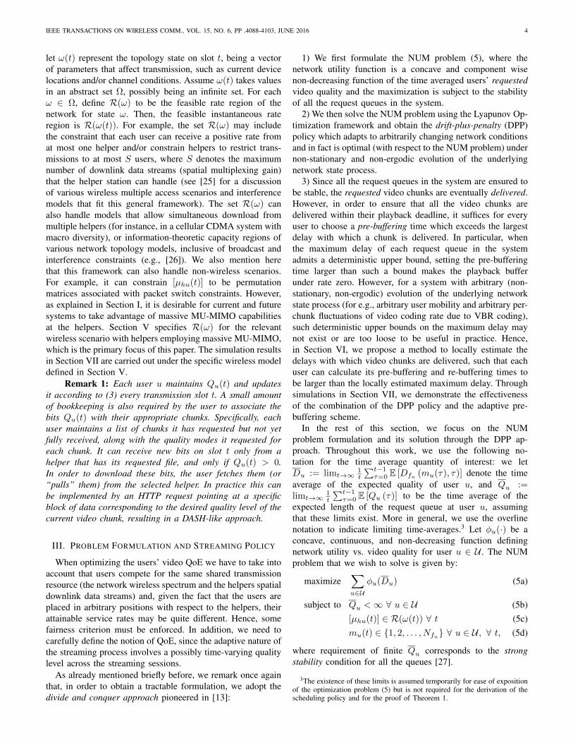
An example of the playback buffer dynamics is illustrated inTable I and Fig. 1. The table indicates the chunk numbers andtheir respective arrival times. The blue curve in Fig. 1 showsthe time evolution of the number of chunks downloaded inthe playback buffer. The green curve indicates the evolutionwith time of the number of chunks consumed by playback.The playback consumption starts after an initial pre-bufferingdelay Tu = d, as indicated in the figure. At any video chunkslot i, the chunk requested at i−d is expected to be available inthe playback buffer. However, if the chunk is delivered with adelay greater than d, the two curves meet and a buffer underrunevent occurs. In order to prevent these events, each user ushould choose its pre-buffering time Tu to be larger than themaximum delay.

More formally, the goal here is to determine the delay Tuafter which user u should start playback, with respect to the

time at which the first chunk is requested (beginning of thestreaming session). We define the size of the playback bufferΨu(i) as the number of chunks available in the buffer at videochunk slot i but not yet played out. Without loss of generality,assume that the streaming session starts at i = 1. Then, Ψu(i)evolves at the video timescale over video chunk slots i ∈1, 2, 3, . . . as:

Ψu(i) = max Ψu(i− 1)− 1i > Tu, 0+ ai. (44)

where 1K denotes the indicator function of a condition orevent K and ai is the number of chunks which are completelydownloaded in the transmission slots between t = (i − 1)nand t = in. Note that the playback buffer is updated everyvideo chunk slot i, i.e., at the time scale of seconds. Thus,if the download of a chunk is completed between t = (i −1)n and t = in, from the playback buffer’s perspective, thechunk is considered to have arrived at the end of the i-thvideo chunk slot, i.e., at t = in. Let Ak denote the videochunk slot in which chunk k arrives at the user and let Wk

denote the delay (measured in video chunk slots) with whichchunk k is delivered. Note that the longest period during whichΨu(i) is not incremented is given by the maximum delay todeliver chunks. Thus, each user u needs to adaptively estimateWk in order to choose Tu. In the proposed method, at eachvideo chunk slot i = 1, 2, . . ., user u calculates the maximumobserved delay Ei in a sliding window of size ∆, by letting:

Ei = maxWk : i−∆ + 1 ≤ Ak ≤ i. (45)

Finally, user u starts its playback when Ψi crosses the levelρEi, i.e., Tu = mini : Ψu(i) ≥ ρEi where ρ is analgorithm control parameter. If a stall event occurs at videochunk slot T , i.e., Ψi = 0 for i > T , the algorithm enters a re-buffering phase in which the same algorithm presented aboveis employed again to determine the new instant T +Tu + 1 atwhich playback is restarted. With slight abuse of notation, were-use Tu to denote the re-buffering delay although it is re-estimated using the sliding window method at each new stallevent.

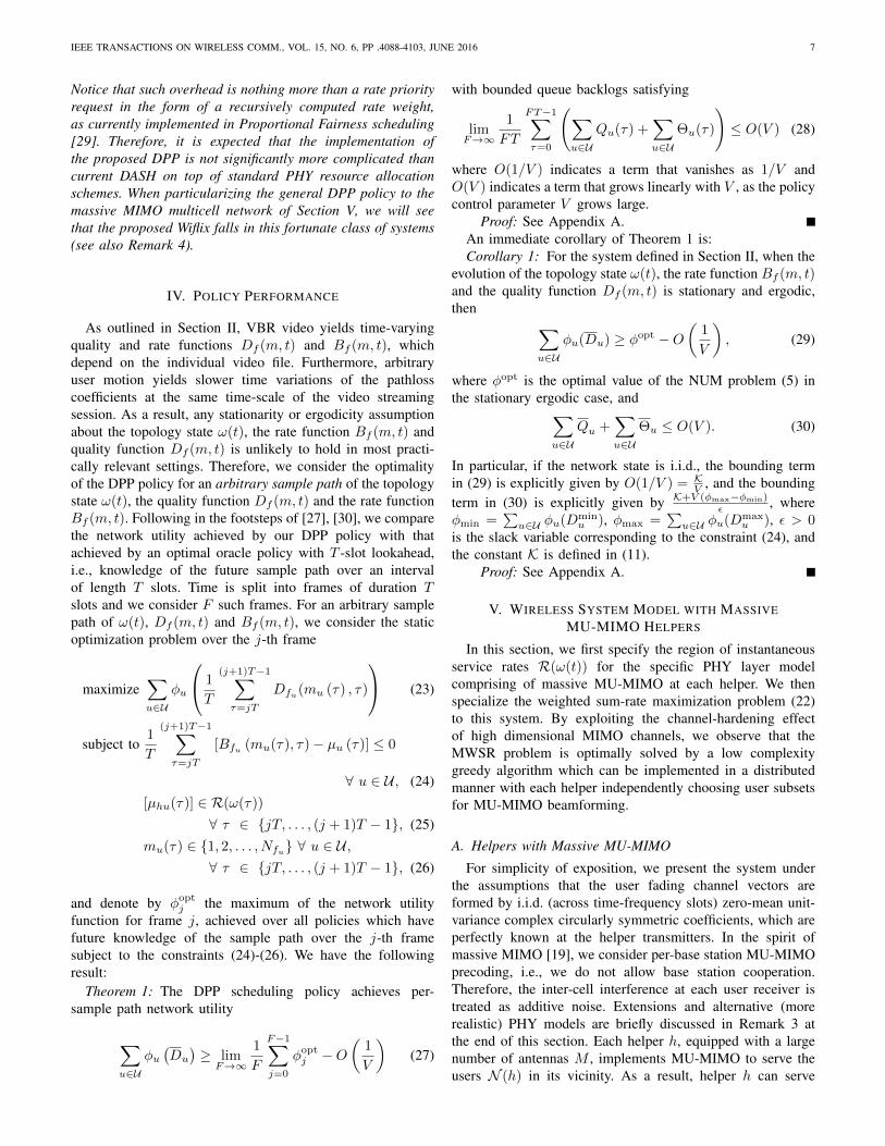
VII. NUMERICAL EXPERIMENT

Our simulations are based on a network topology formedby a 80m×80m region with 5 helpers (indicated by ’s) asshown in Fig. 2. The users (indicated by ∗’s) are generatedaccording to a non-homogeneous Poisson point process withhigher density in a central region of size 80

3 m× 803 m, as shown

in Fig. 2.Each helper has M antennas and serves user sets of size upto

S, with transmission power of 35dBm. The pathloss from ahelper to a user is given by 1

1+( d40 )3.5 , with d representing the

helper-user distance (assuming a torus wrap-around model toavoid boundary effects). We assume a PHY fame duration of10 ms and a total system bandwidth of 18 Mhz as specified inthe LTE 4G standard. With one OFDM resource block (7×12channel symbols) spanning 0.5 ms in time and 180 Khz inbandwidth (corresponding to 12 adjacent subcarriers each with15 KHz bandwidth), each transmission slot spans s = 84 ×100× 20 channel symbols.


TABLE I: Arrival times of chunks

Chunk number 1 2 3 4 5 6 7 8 9 10 11 12 13Arrival time 3 4 6 9 10 11 12 13 16 17 19 20 21

1 2 3 4 5 6 7 8 9 10 11 12 13

1

2

3

4

5

6

7

8

d

video chunk slot (i)

nu

mb

er

of

ch

un

ks

no. of chunks downloaded in the playback buffer

no.of chunks consumed by playback

Fig. 1: Evolution of number of ordered and consumed chunks

0 10 20 30 40 50 60 70 800

10

20

30

40

50

60

70

80

Fig. 2: Simulation setup

We assume that all the users request chunks successivelyfrom VBR-encoded video sequences. Each video file is a longsequence of chunks, each of duration 0.5 seconds and with aframe rate 30 frames per second. We consider a specific videosequence formed by 800 chunks, constructed using severalstandard video clips from the database in [43]. The chunksare encoded into different quality modes with the quality indexmeasured using the Structural SIMilarity (SSIM) index definedin [44]. The chunks from 1 to 200 are encoded into 8 qualitymodes with an average bitrate of 631 kbps. Chunks 201 to 400are encoded in 4 quality modes at an average bitrate of 3908kbps. Similarly, chunks 401−600 and 601−800 are encodedinto 4 and 8 quality modes with average bitrates of 6679 kbpsand 556 kbps respectively. In the simulation, each user starts itsstreaming session of 1000 chunks from some arbitrary positionin this reference video sequence and successively requests1000 chunks by cycling through the sequence.

We choose the utility function Φu(·) = log(·) ∀ u ∈ Uto impose proportional fairness. We set the pre-bufferingalgorithm control parameter (described in Section VI) ρ = 3.We simulate our algorithm for the layout shown in Fig. 2 (witharound 500 users generated according to a non-homogenousPoisson point process as explained above). At t = 1, all theusers simultaneously start streaming 1000 chunks.

We studied the performance of our algorithm with M =40 antennas and maximum active user subset size S = 10for different values of the policy control parameter V and

observed that both the QoE metrics average video quality andthe % of time spent in buffering mode are satisfactory for thechoice of V = 2 ∗ 1014. We use that value for the rest of thesimulations in this section.

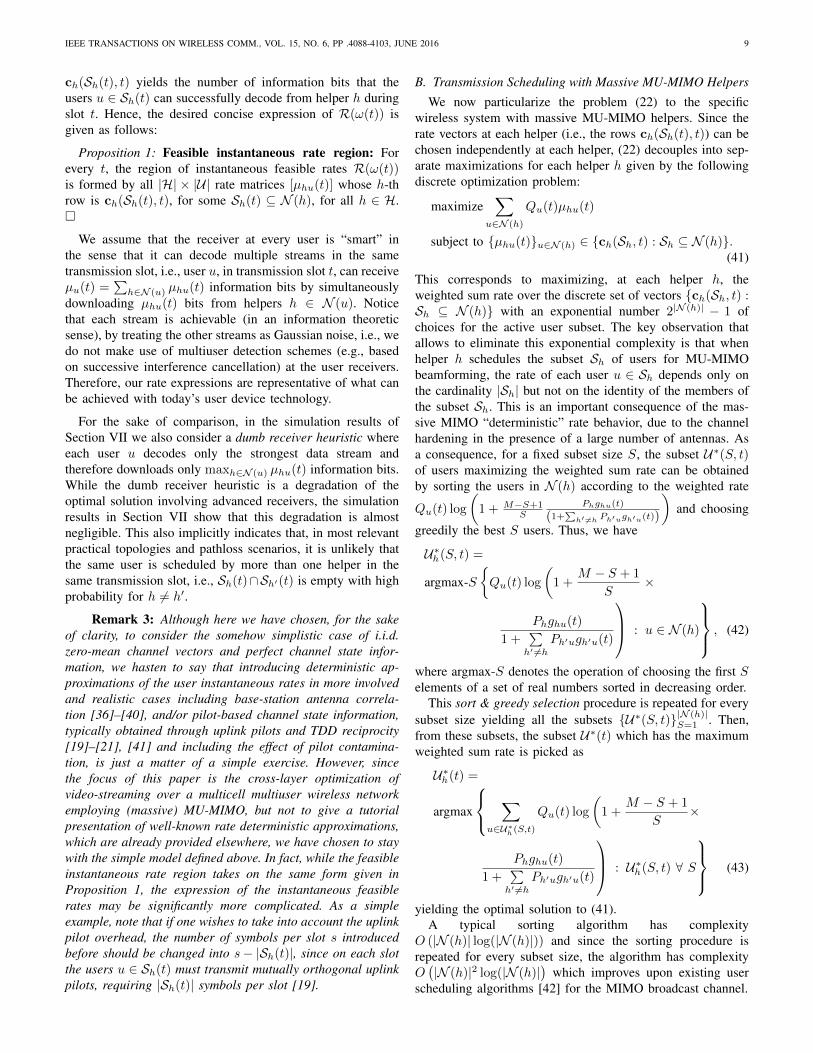
We now study the performance loss experienced underthe dumb receiver heuristic where the receiver at every useru decodes only the strongest signal and downloads onlymaxh∈N (u) µhu(t) in contrast to the macro diversity advancedreceiver which can decode multiple signals simultaneouslyand download all the

∑h∈N (u) µhu(t) bits. Using M = 40

and S = 10, we simulate our algorithm and plot the CDF’sover the user population of a) the average video quality b)the average delay in the reception of video chunks measuredin video chunk slots and c) the % of playback time spent inbuffering mode in Figs. 3a, 3b and 3c respectively. We observethat the performance loss in using a dumb receiver is fairlynegligible and therefore use a dumb receiver for the rest ofthe simulations in this section.

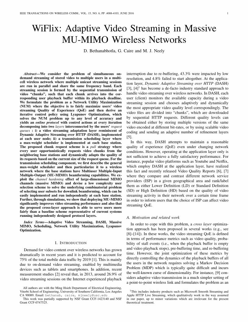
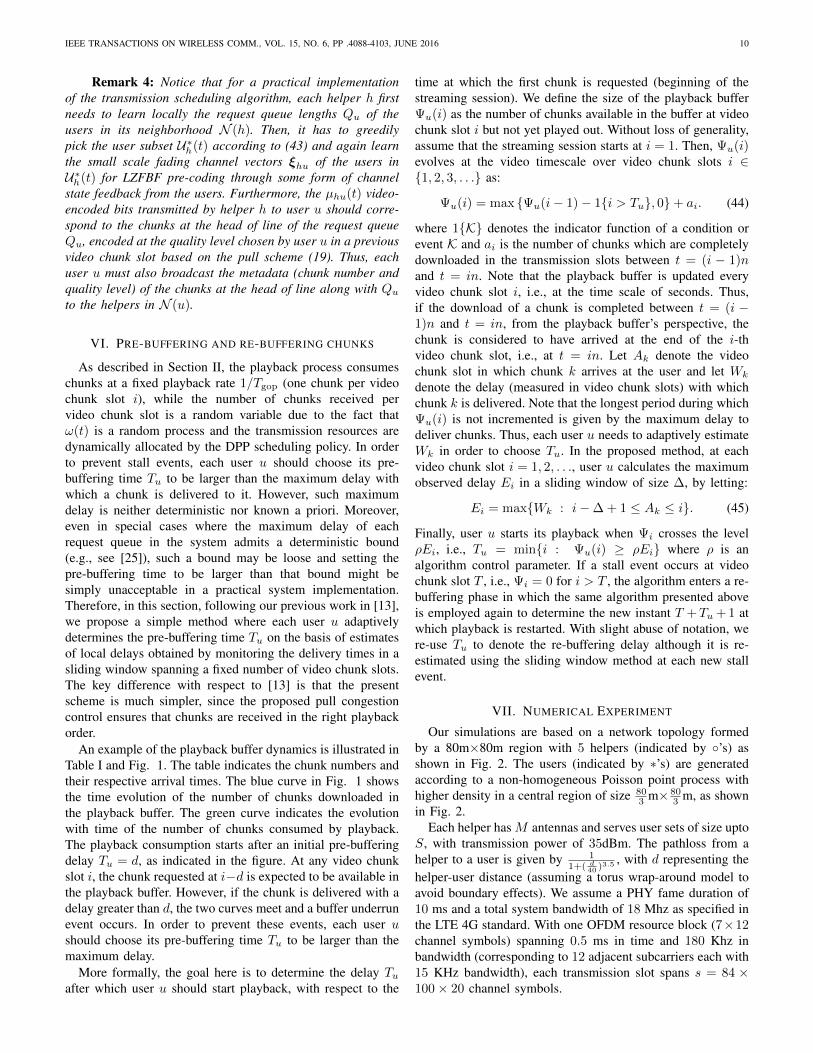
We next study the QoE improvement when MU-MIMOis deployed at the helpers in place of legacy single-userMIMO (SU-MIMO) systems. We plot the CDF over the userpopulation of the same video streaming QoE metrics as inthe previous figures for three different cases 1) MU-MIMOwith M = 40 antennas and maximum active user subsetsize S = 10; 2) MU-MIMO with M = 20 antennas andmaximum active user subset size S = 5; 3) SU-MIMOwith M = 10 antennas. From Figs. 4a, 4c and 4b, wecan observe that there is significant improvement of videostreaming performance in terms of the average video quality,the average delay (or alternately the percentage of time spentin buffering mode) when MU-MIMO is employed at the PHYlayer in comparison to SU-MIMO. This clearly indicates thatupgrading current SU-MIMO systems to massive MU-MIMOis a promising approach to meet the increasing demands forHD video streaming.

Finally, we study the benefits of using a cross layer ap-proach in comparison to a baseline scheme representative oflegacy wireless systems. We perform this comparison for thecase where every helper employs SU-MIMO with M = 10antennas. For the baseline scheme, every user first fixes its


0.89 0.895 0.9 0.905 0.91 0.915 0.92 0.925 0.930

0.1

0.2

0.3

0.4

0.5

0.6

0.7

0.8

0.9

1

video quality averaged over delivered chunks(x)

fra

ctio

n o

f u

se

rs w

ith

avg

. vid

eo

qu

alit

y <

x

dumb receiver

advanced receiver

(a)

5 6 7 8 9 10 11 120

0.1

0.2

0.3

0.4

0.5

0.6

0.7

0.8

0.9

1

average delay measured in no. of video chunk slots(x)

fra

ctio

n o

f u

se

rs w

ith

ave

rag

e d

ela

y <

x

dumb receiver

advanced receiver

(b)

1.5 2 2.5 3 3.5 4 4.5 5 5.50

0.1

0.2

0.3

0.4

0.5

0.6

0.7

0.8

0.9

1

pecentage of time spent in buffering mode(x)

fra

ctio

n o

f u

se

rs w

ith

bu

ffe

rin

g p

ece

nta

ge

< x

dumb receiver

advanced receiver

(c)

Fig. 3: Performance comparison of advanced and dumb receivers.

0.8 0.82 0.84 0.86 0.88 0.9 0.92 0.940

0.1

0.2

0.3

0.4

0.5

0.6

0.7

0.8

0.9

1


fra

ctio

n o

f u

se

rs w

ith

avg

. vid

eo

qu

alit

y <

x

Empirical CDF

MU−MIMO: M=40, S=10


SU−MIMO: M=10, S=1

(a)

0 50 100 150 200 250 3000

0.1

0.2

0.3

0.4

0.5

0.6

0.7

0.8

0.9

1


fra

ctio

n o

f u

se

rs w

ith

avg

. d

ela

y <

x




(b)

0 10 20 30 40 50 60 70 80 90 1000

0.1

0.2

0.3

0.4

0.5

0.6

0.7

0.8

0.9

1

pecentage of time spent in buffering mode(x)

fra

ctio

n o

f u

se

rs w

ith

bu

ffe

rin

g p

ece

nta

ge

< x

Empirical CDF




(c)

Fig. 4: Video streaming QoE improvement with MU-MIMO over SU-MIMO

0.76 0.78 0.8 0.82 0.84 0.86 0.88 0.90

0.1

0.2

0.3

0.4

0.5

0.6

0.7

0.8

0.9

1


fra

ctio

n o

f u

se

rs w

ith

avg

. vid

eo

qu

alit

y <

x

baseline

cross layer

(a)

0 100 200 300 400 500 6000

0.1

0.2

0.3

0.4

0.5

0.6

0.7

0.8

0.9

1


fra

ctio

n o

f u

se

rs w

ith

avg

. d

ela

y <

x

baseline

cross layer

(b)

Fig. 5: Performance comparison of a cross-layer approach with a baseline scheme.

association with the unique helper that provides the maximumreceived signal strength (RSSI) Phghu and then uses thesame control decision (19) to choose the quality levels forthe chunks that arrive into the request queue every videochunk slot. Furthermore, we assume that the helpers locallyemploy Proportional Fairness scheduling [29], which underthe massive MIMO deterministic rate approximation reducesto equal air-time scheduling. In brief, each helper h schedulesthe users associated with it through the max-RSSI scheme in around-robin fashion across the transmission slots independentof the request queue lengths at the users. This baseline

scheme is representative of current practical systems wherethe decisions across different layers are independent and thereis no interaction between the upper and lower layers. We plotthe CDFs over the user population of the average video qualityand the average delay in the reception of chunks in Figs. 5aand 5b respectively. We can observe that the cross layerscheme treats the users in a fair manner while the baselinescheme favors some users at the expense of other users in thesystem. Since the topology in Fig. 2 has a central region withhigher user density (hotspot) and the user-helper associationis max-RSSI based in the baseline scheme, most of the users


in the hotspot get associated to the helper in the center ofthe topology. As a consequence, this helper get overloadedwith many users associated to it. Moreover, since the helperemploys the round-robin scheduling policy in the baselinescheme, each user in the hotspot gets scheduled only on asmall fraction of transmission slots resulting in poor videoquality and delay performance. However, the users which areoutside the hotspot get associated to the lightly loaded helpersand therefore experience better video streaming QoE. Thisexplains the skewed nature of the distributions in Figs. 5a and5b corresponding to the baseline scheme.

On the other hand, with the cross-layer scheme, the user-helper association is dynamic and it changes during the courseof control policy depending on the transmission schedulingdecisions which in turn depend on the achievable rates of theusers and their dynamically changing request queue lengths.Such dynamic user-helper association implicitly balances theload across all the helpers in the system leading to fairness inQoE performance across the user population.

VIII. CONCLUSIONS

In this work we propose WiFlix, a system for efficientstreaming of video content in a network of helpers capable ofimplementing the advanced physical layer technique massiveMU-MIMO. We formulate a NUM problem to maximize thevideo streaming QoE of the users in the network and solve itusing the Lyapunov Optimization technique to derive a controlpolicy which decomposes into congestion control decisions atthe users and transmission scheduling decisions at the helpers.We devise a low complexity greedy user selection schemeto solve optimally the combinatorial problem of schedulingusers for multiuser beamforming. The transmission schedulingdecisions consist of each base station choosing the subset ofusers for MU-MIMO beamforming. By exploiting the channelhardening effect of high dimensional MIMO channels, wereduce the combinatorial weighted sum rate maximizationover the multiuser multicell network (which would involvean exponentially complex exhaustive user selection, or somepolynomial complexity heuristic greedy user selection at eachbase station) to a simple subset selection problem which is op-timally solved by a low complexity algorithm. The algorithm isamenable to easy implementation with local, independent userscheduling decisions at the helpers. Similarly, the congestioncontrol decisions can be implemented independently at theusers with each user opportunistically pulling chunks from itsneighboring helpers and adapting the quality of the chunk re-quests in response to changing network conditions reflected bychanging request queue sizes. Possible future considerationsinclude implementing and testing WiFlix in practice.

APPENDIX APROOF OF THEOREM 1 AND OF COROLLARY 1

As in Section III, we consider the following problem,equivalent to (23) – (26), which involves a sum of time-averages instead of functions of time averages and introduces

the auxiliary variables γu(t):

maximize1

T

(j+1)T−1∑τ=jT

∑u∈U

φu (γu(τ)) (46a)

subject to1

T

(j+1)T−1∑τ=jT

[Bfu (mu(τ), τ)− µu (τ)] ≤ 0 ∀ u ∈ U

(46b)

1

T

(j+1)T−1∑τ=jT

[γu (τ)−Dfu (mu(τ), τ)] ≤ 0 ∀ u ∈ U

(46c)

Dminu ≤ γu(τ) ≤ Dmax

u ∀ u ∈ U ,∀ τ ∈ jT, . . . , (j + 1)T − 1

(46d)[µhu(τ)] ∈ R(ω(τ)) ∀ τ ∈ jT, . . . , (j + 1)T − 1

(46e)mu(τ) ∈ 1, 2, . . . , Nfu ∀ u ∈ U ,

∀ τ ∈ jT, . . . , (j + 1)T − 1(46f)

The update equations for the request queues Qu ∀ u ∈ Uand the virtual queues Θu ∀ u ∈ U are given in (3)

and in (7), respectively. Let G(τ) =[QT(τ),ΘT(τ)

]Tbe

the combined queue backlogs column vector, and define thequadratic Lyapunov function L(G(τ) = 1

2GT(τ)G(τ). Fix aparticular slot τ in the j-th frame. We first consider the one-slot drift of L(G(τ)). From (15), we know that

L(G(τ + 1))− L(G(τ)) ≤ K + (B(τ)− µ(τ))T

Q(τ)

+ (γ(τ)−D(τ))T

Θ(τ)(47)

where K is a uniform bound on the term

1

2

[(B(τ)− µ(τ))

T(B(τ)− µ(τ))

+ (γ(τ)−D(τ))T

(γ(τ)−D(τ))]

(48)

, which exists under the realistic assumption that the chunksizes, the transmission rates and the video quality measuresare upper bounded by some constants, independent of τ . Wechoose K such that

K > 2κTκ (49)

where κ is a vector whose components are all equal to thesame number κ and this number is a uniform upper bound onthe maximum possible magnitude of drift in any of the queues(both the request queues Qu and the virtual queues Θu) in oneslot. With the additional penalty term −V

∑u∈U φu(γu(τ))

added on both sides of (47), we have the following DPPinequality:


L(G(τ + 1))− L(G(τ))− V∑u∈U

φu(γu(τ))

≤ K + (B(τ)− µ(τ))T

Q(τ) + (γ(τ)−D(τ))T

Θ(τ)

− V∑u∈U

φu(γu(τ)) (50)

Let the DPP policy which minimizes the right hand sideof the drift-plus-penalty inequality (50) comprise of the con-trol actions mu(τ)(j+1)T−1

τ=jT ∀ u ∈ U , γ(τ)(j+1)T−1τ=jT

and (µhu(τ))(j+1)T−1τ=jT . Since the DPP policy minimizes

the expression on the RHS of (50), any other policy com-prising of the control actions m∗u(τ)(j+1)T−1

τ=jT ∀ u ∈U , γ∗(τ)(j+1)T−1

τ=jT and (µ∗hu(τ))(j+1)T−1τ=jT would give a

larger value of the expression. We therefore have

L(G(τ + 1))− L(G(τ))− V∑u∈U

φu(γu(τ))

≤ K + (B∗(τ)− µ∗(τ))T

Q(τ) + (γ∗(τ)−D∗(τ))T

Θ(τ)

− V∑u∈U

φu(γ∗u(τ)). (51)

Further, we note that the maximum change in the queuelength vectors Qu(τ) and Θu(τ) from one slot to the next isbounded by κ. Thus, we have for all τ ∈ jT, . . . , (j+1)T −1

|Qu(τ)−Qu(jT )| ≤ (τ − jT )κ ∀ u ∈ U (52)|Θu(τ)−Θu(jT )| ≤ (τ − jT )κ ∀ u ∈ U (53)

Substituting the above inequalities in (51), we have

L(G(τ + 1))− L(G(τ))− V∑u∈U

φu(γu(τ))

≤ K + (B∗(τ)− µ∗(τ))T

(Q(jT ) + (τ − jT )κ)

+ (γ∗(τ)−D∗(τ))T

(Θ(jT ) + (τ − jT )κ)

− V∑u∈U

φu(γ∗u(τ)). (54)

Then, summing (54) over τ ∈ jT, . . . , (j + 1)T − 1, weobtain the T -slot Lyapunov drift over the j-th frame:

L(G((j + 1)T ))− L(G(jT ))− VjT+T−1∑τ=jT

∑u∈U

φu(γu(τ))

≤ KT +

(∑jT+T−1

τ=jT(B∗(τ)− µ∗(τ))

)T

Q(jT )

+

(∑jT+T−1

τ=jT(B∗(τ)− µ∗(τ)) (τ − jT )

)T

κ

+

(∑jT+T−1

τ=jT(γ∗(τ)−D∗(τ))

)T

Θ(jT )

+

(∑jT+T−1

τ=jT(γ∗(τ)−D∗(τ)) (τ − jT )

)T

κ

− V∑jT+T−1

τ=jT

∑u∈U

φu(γ∗u(τ)) (55)

Using the inequalities B∗(τ) − µ∗(τ) ≤ 2κ, γ∗(τ) −D∗(τ) ≤ 2κ in (55), we have


∑u∈U

φu(γu(τ))

≤ KT +

(∑jT+T−1

τ=jT(B∗(τ)− µ∗(τ))

)T

Q(jT )

+ 2

(∑jT+T−1

τ=jT(τ − jT )

)κTκ

+

(∑jT+T−1


)T

Θ(jT )

+ 2

(∑jT+T−1

τ=jT(τ − jT )

)κTκ

− V∑jT+T−1

τ=jT

∑u∈U

φu(γ∗u(τ)) (56)

Using κTκ ≤ K2 ,∑jT+T−1τ=jT (τ − jT ) = T (T−1)

2 , we get


∑u∈U

φu(γu(τ))

≤ KT 2 +

(∑jT+T−1

τ=jT(B∗(τ)− µ∗(τ))

)T

Q(jT )

+

(∑jT+T−1


)T

Θ(jT )

− V∑jT+T−1

τ=jT

∑u∈U

φu(γ∗u(τ)) (57)

We now consider the policy comprising of the controlactions m∗u(τ)(j+1)T−1

τ=jT ∀ u ∈ U , γ∗(τ)(j+1)T−1τ=jT and

(µ∗hu(τ))(j+1)T−1τ=jT , and satisfying the following constraints:4

1

T

(j+1)T−1∑τ=jT

[B∗fu (mu(τ), τ)− µ∗u (τ)

]< −ε ∀ u ∈ U (58)

1

T

(j+1)T−1∑τ=jT

[γ∗u (τ)−D∗fu (mu(τ), τ)

]< −ε ∀ u ∈ U (59)

where ε > 0 is arbitrary. We plug in the inequalities (58),(59) in (57) and obtain

4It is easy to see that such policy is guaranteed to exist provided that weallow, without loss of generality, for a virtual video layer of zero quality andzero rate, and in the assumption that, at any slot t, each user u has at least onelink (h, u) ∈ E with h ∈ N (u) ∩ H(fu) with peak rate lower bounded bysome strictly positive number Cmin. This prevents the case where a user getszero rate for a whole frame of length T . This assumption is not restrictivein practice since a user experiencing unacceptably poor link quality to all thehelpers for a long time interval would be disconnected from the network andits streaming session halted.



∑u∈U

φu(γu(τ))

< KT 2 − εT∑u∈U

Qu(jT )− εT∑u∈U

Θu(jT )

− V∑jT+T−1

τ=jT

∑u∈U

φu(γ∗u(τ)) (60)

Also, considering the fact that for any vector γ =(γ1, . . . , γ|U|) we have∑

u∈Uφu(Dmin

u ) = φmin ≤∑u∈U

φu(γu)

≤ φmax =∑u∈U

φu(Dmaxu ), (61)

we can write:

L(G((j + 1)T ))− L(G(jT ))

< KT 2 + V T (φmax − φmin)− εT∑u∈U

Qu(jT )

− εT∑u∈U

Θu(jT ) (62)

Once again using (52), (53), we have:

L(G((j + 1)T ))− L(G(jT ))

< KT 2 + V T (φmax − φmin)− εjT+T−1∑τ=jT

∑u∈U

Qu(τ)

− εjT+T−1∑τ=jT

∑u∈U

Θu(τ) + εκ|U|T (T − 1) (63)

Summing the above over the frames j ∈ 0, . . . , F −1 yields

L(G((FT ))− L(G(0))

< KT 2F + V FT (φmax − φmin)− εFT−1∑τ=0

∑u∈U

Qu(τ)

− εFT−1∑τ=0

∑u∈U

Θu(τ) + εκ|U|FT (T − 1) (64)

Rearranging and neglecting appropriate terms, we get

1

FT

FT−1∑τ=0

∑u∈U

Qu(τ) +1

FT

FT−1∑τ=0

∑u∈U

Θu(τ)

<KTε

+V (φmax − φmin)

ε+L(G(0))

εFT+ κ|U|(T − 1)

(65)

Taking limits as F →∞

limF→∞

1

FT

FT−1∑τ=0

(∑u∈U

Qu(τ) +∑u∈U

Θu(τ)

)

<KTε

+V (φmax − φmin)

ε+ κ|U|(T − 1) (66)

such that (28) is proved.

We now consider the policy comprising of the decisionswhich achieves the optimal solution φoptj to the problem (46a)– (46e). Using (46b) and (46c) in (57), we have


∑u∈U

φu(γu(τ))

≤ KT +KT (T − 1)− V Tφoptj

(67)

Summing this over j ∈ 0, . . . , F − 1, yields

L(G((FT ))− L(G(0))− VFT−1∑τ=0

∑u∈U

φu(γu(τ))

≤ KT 2F − V TF−1∑j=0

φoptj . (68)

Dividing both sides by V FT and using the fact thatL(G((FT )) > 0 , we get

1

FT

FT−1∑τ=0

∑u∈U

φu(γu(τ)) ≥ 1

F

F−1∑j=0

φoptj − KTV− L(G(0))

V TF.

(69)

At this point, using Jensen’s inequality, the fact that φu(·)is continuous and non-decreasing for all u ∈ U , and thefact that the strong stability of the queues (66) implies thatlimF→∞

1FT

∑FT−1τ=0 Θu(τ) < ∞ ∀ u ∈ U , which in turns

implies that γu ≤ Du ∀ u ∈ U , we arrive at

∑u∈U

φu(Du

)≥ limF→∞

1

F

F−1∑j=0

φoptj − KTV. (70)

such that (27) is proved.Thus, the utility under the DPP policy is within O(1/V ) of

the time average of the φoptj utility values that can be achievedonly if knowledge of the future states up to a look-ahead ofblocks of T slots. If T is increased, then the value of φoptj forevery frame j improves since we allow a larger look-ahead.However, from (70), we can see that if T is increased, then Vcan also be increased in order to maintain the same distancefrom optimality. This yields a corresponding O(V ) increasein the queues backlog.

For the case where the rate function Bf (m, t), the qualityfunction Df (m, t) and the topology state ω(t)is stationary andergodic, the time average in the left hand side of (66) and inthe right hand side of (70) become ensemble averages becauseof ergodicity. Thus, we obtain (29) and (30). Furthermore, ifthe network state is i.i.d., we can take T = 1 in the abovederivation, obtaining the bounds given in Corollary 1.

REFERENCES

[1] “Cisco visual networking index: Global mobile data traffic forecastupdate, 2014-2019.” [Online]. Available: http://goo.gl/1XYhqY

[2] “Conviva viewer experience report, 2014.” [Online]. Available:http://www.conviva.com/vxr/

[3] “MPEG DASH standard.” [Online]. Available: http://dashif.org/mpeg-dash

[4] A. Begen, T. Akgul, and M. Baugher, “Watching video over the web:Part 1: Streaming protocols,” Internet Computing, IEEE, vol. 15, no. 2,pp. 54–63, 2011.


[5] Y. Sanchez, T. Schierl, C. Hellge, T. Wiegand, D. Hong,D. De Vleeschauwer, W. Van Leekwijck, and Y. Lelouedec, “iDASH:improved dynamic adaptive streaming over http using scalable videocoding,” in ACM Multimedia Systems Conference (MMSys), 2011, pp.23–25.

[6] “Google video quality report.” [Online]. Available: https://www.google.com/get/videoqualityreport/

[7] “Netflix ISP speed index.” [Online]. Available: http://ispspeedindex.netflix.com/

[8] V. Joseph and G. de Veciana, “Nova: Qoe-driven optimization of dash-based video delivery in networks,” arXiv preprint arXiv:1307.7210,2013.

[9] C. Gong and X. Wang, “Adaptive transmission for delay-constrainedwireless video,” Wireless Communications, IEEE Transactions on,vol. 13, no. 1, pp. 49–61, January 2014.

[10] A. A. Khalek, C. Caramanis, and R. W. Heath Jr, “Loss visibilityoptimized real-time video transmission over mimo systems,” arXivpreprint arXiv:1301.3174, 2013.

[11] M. Zhao, X. Gong, J. Liang, W. Wang, X. Que, and S. Cheng, “Schedul-ing and resource allocation for wireless dynamic adaptive streamingof scalable videos over http,” in Communications (ICC), 2014 IEEEInternational Conference on, June 2014, pp. 1681–1686.

[12] C. Chen, R. Heath, A. Bovik, and G. de Veciana, “Adaptive policies forreal-time video transmission: A markov decision process framework,”in Image Processing (ICIP), 2011 18th IEEE International Conferenceon. IEEE, 2011, pp. 2249–2252.

[13] D. Bethanabhotla, G. Caire, and M. J. Neely, “Adaptive video streamingfor wireless networks with multiple users and helpers,” Communications,IEEE Transactions on, vol. 63, no. 1, pp. 268–285, Jan 2015.

[14] K. Miller, D. Bethanabhotla, G. Caire, and A. Wolisz, “A control-theoretic approach to adaptive video streaming in dense wireless net-works,” Multimedia, IEEE Transactions on, vol. 17, no. 8, pp. 1309–1322, 2015.

[15] “IEEE 802.11ac - Wikipedia,” https://en.wikipedia.org/wiki/IEEE 802.11ac, Last Updated: January 14, 2014.

[16] J. Andrews, S. Buzzi, W. Choi, S. Hanly, A. Lozano, A. Soong, andJ. Zhang, “What will 5G be?” Selected Areas in Communications, IEEEJournal on, vol. 32, no. 6, pp. 1065–1082, June 2014.

[17] D. Bethanabhotla, O. Y. Bursalioglu, H. C. Papadopoulos, and G. Caire,“Optimal user-cell association for massive MIMO wireless networks,”Wireless Communications, IEEE Transactions on, vol. PP, no. 99, pp.1–1, 2015.

[18] “pCell white paper.” [Online]. Available: http://goo.gl/lDrofd[19] T. L. Marzetta, “Noncooperative cellular wireless with unlimited num-

bers of base station antennas,” IEEE Trans. on Wireless Communications,vol. 9, no. 11, pp. 3590–3600, Nov. 2010.

[20] H. Huh, G. Caire, H. Papadopoulos, and S. Ramprashad, “Achievingmassive MIMO spectral efficiency with a not-so-large number of an-tennas,” IEEE Trans. on Wireless Communications, vol. 11, no. 9, pp.3226–3239, 2012.

[21] J. Hoydis, S. Ten Brink, and M. Debbah, “Massive MIMO in the UL/DLof cellular networks: How many antennas do we need?” Selected Areasin Communications, IEEE Journal on, vol. 31, no. 2, pp. 160–171, 2013.

[22] A. Ortega, “Variable bit-rate video coding,” Compressed Video overNetworks, pp. 343–382, 2000.

[23] Z. Wang, A. C. Bovik, H. R. Sheikh, and E. P. Simoncelli, “Imagequality assessment: From error visibility to structural similarity,” ImageProcessing, IEEE Transactions on, vol. 13, no. 4, pp. 600–612, 2004.

[24] A. F. Molisch, Wireless communications. Wiley, 2010, vol. 15.[25] M. J. Neely, “Wireless peer-to-peer scheduling in mobile networks,”

in 2012 46th Annual Conference on Information Sciences and Systems(CISS). IEEE, 2012, pp. 1–6.

[26] A. El Gamal and Y. Kim, “Lecture notes on network information theory,”Arxiv preprint arxiv:1001.3404, vol. 3, 2010.

[27] M. Neely, “Stochastic network optimization with application to commu-nication and queueing systems,” Synthesis Lectures on CommunicationNetworks, vol. 3, no. 1, pp. 1–211, 2010.

[28] J. Mo and J. Walrand, “Fair end-to-end window-based congestioncontrol,” IEEE/ACM Transactions on Networking (ToN), vol. 8, no. 5,pp. 556–567, 2000.

[29] A. Eryilmaz and R. Srikant, “Fair resource allocation in wireless net-works using queue-length-based scheduling and congestion control,” inINFOCOM 2005. 24th Annual Joint Conference of the IEEE Computerand Communications Societies. Proceedings IEEE, vol. 3. IEEE, 2005,pp. 1794–1803.

[30] M. Neely, “Universal scheduling for networks with arbitrary traffic,channels, and mobility,” in Decision and Control (CDC), 2010 49thIEEE Conference on. IEEE, 2010, pp. 1822–1829.

[31] A. Tulino and S. Verdu, Random matrix theory and wireless communi-cations. Now Publishers Inc, 2004, vol. 1.

[32] R. Couillet and M. Debbah, Random matrix methods for wirelesscommunications. Cambridge University Press, 2011.

[33] H. Huh, A. M. Tulino, and G. Caire, “Network MIMO with linearzero-forcing beamforming: Large system analysis, impact of channelestimation, and reduced-complexity scheduling,” Information Theory,IEEE Transactions on, vol. 58, no. 5, pp. 2911–2934, 2012.

[34] Y. Lim, C. Chae, and G. Caire, “Performance analysis of massive MIMOfor cell-boundary users,” Wireless Communications, IEEE Transactionson, vol. PP, no. 99, pp. 1–1, 2015.

[35] B. Hassibi and B. M. Hochwald, “How much training is needed inmultiple-antenna wireless links?” Information Theory, IEEE Transac-tions on, vol. 49, no. 4, pp. 951–963, 2003.

[36] A. Adhikary, J. Nam, J.-Y. Ahn, and G. Caire, “Joint spatial divisionand multiplexingthe large-scale array regime,” IEEE Trans. on Inform.Theory, vol. 59, no. 10, pp. 6441–6463, 2013.

[37] J. Nam, A. Adhikary, J.-Y. Ahn, and G. Caire, “Joint spatial division andmultiplexing: Opportunistic beamforming, user grouping and simplifieddownlink scheduling,” IEEE J. of Sel. Topics in Sig. Proc. (JSTSP),vol. 8, no. 5, pp. 876–890, 2014.

[38] A. Adhikary, E. Al Safadi, M. K. Samimi, R. Wang, G. Caire, T. S.Rappaport, and A. F. Molisch, “Joint spatial division and multiplexingfor mm-wave channels,” IEEE J. on Sel. Areas on Commun. (JSAC),vol. 32, no. 6, pp. 1239–1255, 2014.

[39] H. Yin, D. Gesbert, M. Filippou, and Y. Liu, “A coordinated approachto channel estimation in large-scale multiple-antenna systems,” SelectedAreas in Communications, IEEE Journal on, vol. 31, no. 2, pp. 264–273,2013.

[40] S. Wagner, R. Couillet, M. Debbah, and D. Slock, “Large systemanalysis of linear precoding in correlated miso broadcast channels underlimited feedback,” Information Theory, IEEE Transactions on, vol. 58,no. 7, pp. 4509–4537, 2012.

[41] H. Q. Ngo, E. G. Larsson, and T. L. Marzetta, “Energy and spectralefficiency of very large multiuser mimo systems,” Communications,IEEE Transactions on, vol. 61, no. 4, pp. 1436–1449, 2013.

[42] T. Yoo and A. Goldsmith, “On the optimality of multiantenna broadcastscheduling using zero-forcing beamforming,” Selected Areas in Commu-nications, IEEE Journal on, vol. 24, no. 3, pp. 528–541, 2006.

[43] http://media.xiph.org/video/derf/.[44] “The SSIM Index for Image Quality Assessment.” [Online]. Available:

http://goo.gl/ngR0UL

IEEE TRANSACTIONS ON WIRELESS COMM., VOL. 15, NO. 6, PP ...

Documents

Transcript of IEEE TRANSACTIONS ON WIRELESS COMM., VOL. 15, NO. 6, PP ...