IEEE TRANSACTIONS ON MEDICAL IMAGING, VOL. 24, NO. … · DTI Segmentation Using an Information...

IEEE TRANSACTIONS ON MEDICAL IMAGING, VOL. 24, NO. 10, OCTOBER 2005 1267

DTI Segmentation Using an Information TheoreticTensor Dissimilarity Measure

Zhizhou Wang, Member, IEEE, and Baba C. Vemuri*, Fellow, IEEE

Abstract—In recent years, diffusion tensor imaging (DTI) has be-come a popular in vivo diagnostic imaging technique in Radiolog-ical sciences. In order for this imaging technique to be more effec-tive, proper image analysis techniques suited for analyzing thesehigh dimensional data need to be developed.

In this paper, we present a novel definition of tensor “distance”grounded in concepts from information theory and incorporateit in the segmentation of DTI. In a DTI, the symmetric positivedefinite (SPD) diffusion tensor at each voxel can be interpretedas the covariance matrix of a local Gaussian distribution. Thus, anatural measure of dissimilarity between SPD tensors would bethe Kullback-Leibler (KL) divergence or its relative. We proposethe square root of the J-divergence (symmetrized KL) betweentwo Gaussian distributions corresponding to the diffusion tensorsbeing compared and this leads to a novel closed form expressionfor the “distance” as well as the mean value of a DTI. Unlike thetraditional Frobenius norm-based tensor distance, our “distance”is affine invariant, a desirable property in segmentation and manyother applications. We then incorporate this new tensor “distance”in a region based active contour model for DTI segmentation.Synthetic and real data experiments are shown to depict theperformance of the proposed model.

Index Terms—Diffusion tensor MRI, image segmentation,Kullback-Leibler divergence, J-divergence, Mumford-Shah func-tional, active contour.

I. INTRODUCTION

I N [8], Basser et al. presented their seminal work on diffusiontensor magnetic resonance imaging (DT-MRI). Since this

new MRI modality can be used to quantify anisotropic propertiesof the imaged tissue by characterizing the water diffusionthrough the same, it has became a powerful technique toinvestigate the tissue microstructure in vivo, e.g., white matterconnectivity in the brain or in the spinal cord. Investigating thetissue microstructure and changes therein (due to pathology)is achieved via DTI analysis. This in general includes a broadspectrum of interesting problems namely, optimal DT-MRimaging protocol design, DTI restoration, DTI segmentation,DTI registration, DTI visualization and fiber track mapping.

Manuscript received August 7, 2004; revised July 5, 2005. This work wassupported in part by the National Institutes of Health (NIH) under Grant NIHRO1 NS42075. The Associate Editor responsible for coordinating the reviewof this paper and recommending its publication was T. Jiang. Asterisk indicatescorresponding author.

Z. Wang is with Siemens Corporate Research, Inc., Princeton, NJ 08540 USA.*B. C. Vemuri is with the Department of CISE, University of Florida,

Gainesville, FL 32611 USA (e-mail: [email protected]).Digital Object Identifier 10.1109/TMI.2005.854516

In DT-MRI, what is measured is the diffusion weighted echointensity image (DWI) . It can be related to the diffusiontensor through the Stejskal-Tanner equation [8] given by

(1)

where is the diffusion weighting of the -th diffusion en-coding magnetic gradient, “:” denotes the generalized innerproduct for matrices. Given several noncollinear diffusionweighted intensity measurements, can be estimated viamultivariate regression techniques.

One key factor in DTI analysis is a proper choice of diffusiontensor distance that measures the similarity or dissimilarity be-tween the tensors and is particularly important in the aforemen-tioned tasks. In the following, we will present a brief overviewof different tensor distance measures used in DTI analysis andvarious techniques currently in vogue in using tensor-based in-formation for segmenting DTI.

In general, any kind of matrix norm can be used to mea-sure the distance between two 2-tensors. One such example isthe tensor Euclidean distance obtained by using the Frobeniusnorm. Due to its simplicity, tensor Euclidean distance has beenused extensively in DTI restoration [11], [12], [32]. Alexanderet al. [2] considered a number of tensor similarity measuresfor matching diffusion tensor images and concluded empiricallythat the Euclidean difference measure yields the best results.Though not many sophisticated tensor distances have been pro-posed in DTI analysis, there are quite a few in the context ofmachine learning. Miller et al. [22] proposed an interesting mea-sure on transformation groups to design an invariant kernel fornonparametric density estimation. What is most closely relatedto our present work was proposed by Tsuda et al. [29]. Theyintroduced information geometry in the space of positive defi-nite matrices to derive a Kullback-Leibler divergence betweenthem and then used it in an “em” (not the well-known expec-tation-maximization) algorithm to approximate an incompletekernel.

In the context of DTI segmentation, in [33], Wiegell et al. ap-plied the K-means clustering (involves tensor Frobenius norm)technique for segmentation of thalamic nuclei from DTI. Simul-taneously, Zhukov et al. [35] proposed a level set segmentationmethod to segment scalar anisotropic images derived from thediffusion tensor. The fact that such scalar fields are used impliesthat they have ignored the direction information contained in theDTI. Thus, this method will fail if two homogeneous regions ofDTI have the same anisotropy property but are oriented in a to-tally different direction.

0278-0062/$20.00 © 2005 IEEE

1268 IEEE TRANSACTIONS ON MEDICAL IMAGING, VOL. 24, NO. 10, OCTOBER 2005

Prior to our published work in [31], the only published workon the segmentation of matrix-valued images was reported inFeddern et al. [13]. In their work [13], Feddern et al. extendedthegeodesicactivecontoursmodelforapplicationtotensorfields,specifically to the structure tensor field computed from gray scaleimages. The stopping criterion in this case is chosen as a de-creasing function of the trace of the sum of the structure tensorsformed from individual elements of the given tensor in the tensorfield. This amounts to taking the Frobenius norm of the tensors inthe tensorfieldformedbythegradientmagnitudeof the individualchannels/components of the given tensor. This scheme is a gra-dient based active contour(snake) whose performance is lackingin absence of significant gradient in the data. Moreover, the normused here is not invariant to affine transformations of the inputcoordinates on which the original tensor field is defined. Affineinvariance is a desirable property for the segmentation schemewhen dealing with data sets obtained from different hardware.

In [31], we applied a region-based active contour model fortensor field segmentation by incorporating a tensor distancebased on matrix Frobenius norm. Simultaneously, Rousson etal. [25] extended the classical surface evolution segmentationmodel by incorporating region statistics defined on the tensorfields for DTI segmentation. In both works [25], [31], differentcomponents in the diffusion tensor is treated in the same way.However, the diffusion tensor is actually the covariance matrixof a local diffusion process and different components havedifferent importance/weight. The importance of this fact in DTIsegmentation was first recognized by Wang and Vemuri in [30].Specifically, they proposed an information theoretic “distance”for rank 2 tensors and incorporated it in a region-based activecontour model to segment tensor fields. Soon after, Lengletet al. [16], [17] extended the concepts presented in [30] forprobability density field segmentation in a Bayesian frameworkwith application to DTI segmentation.

In this paper, we tackle the DTI segmentation problem usinga region-based active contour model by incorporating an infor-mation theoretic tensor dissimilarity measure. This paper is asignificant extension of our preliminary work reported in [30].Geometric active contour models have long been used in scalarand vector-valued image segmentation [9], [15], [18]–[20]. Ourwork is based on the active contour models derived from theMumford-Shah functional [23], and can be viewed as a signif-icant extension of the work on active contours without edges,by Chan and Vese [10] and the work on curve evolution imple-mentation of the Mumford-Shah functional by Tsai et al. [28] todiffusion tensor images. Our key contributions are: 1) the defi-nition of a new affine invariant discriminant of tensors based oninformation theory; 2) a theorem and its proof that allows forthe computation of the mean value of an SPD tensor field—re-quired in the piecewise constant version of the region-based ac-tive contour model—in closed form and facilitates the efficientsegmentation of the DTI; 3) Derivation of an analytic expres-sion for the derivatives of the energy function in the piecewisesmooth region-based segmentation case; and 4) extension of thepopular region-based active contour model in level-set form tohandle matrix-valued images, e.g., DTI.

The remainder of this paper is organized as follows: inSection II, the new definition of tensor distance is introduced

and its properties are discussed in detail. Then, in Section III-A,the piecewise constant region-based active contour modelfor DTI segmentation is discussed. We present the associ-ated Euler-Lagrange equation, the curve evolution equation,the level set formulation and the implementation details. InSection III-B, we present the piecewise smooth region-basedactive contour model for DTI segmentation. Section IV containsexperiments on application of our model to synthetic tensorfields as well as real DTIs and Section V the conclusion.

II. A NEW TENSOR DISTANCE AND ITS PROPERTIES

We now present the definition and properties of our new “dis-tance” measure between diffusion tensors.

A. Definitions

Given a diffusion tensor , the displacement of watermolecules starts from a given location at time is a randomvariable with the following probability density:

(2)

where is the size of the square matrix . Note that the meanof and the covariance matrix of is[26]. It follows that a natural distance between diffusion tensorscan be derived from an information theoretical distance measurebetween Gaussian distributions. The first choice could be theKullback-Leibler (KL) divergence given as

(3)

for a pair of probability density functions and .However, KL divergence is not symmetric and the most fre-

quently used way to symmetrize it is the J-divergence given by

(4)

We propose a novel definition of diffusion tensor “distance”as the square root of the J-divergence of the correspondingGaussian distributions, i.e.,

(5)

For , and given as in (2), it is knownthat [34]

where is the matrix trace operator.Thus, (5) has a very nice closed form given by

(6)

We use the quotation marks on the distance here because,what we have defined in (6) is not a true distance since it violatesthe triangle inequality. We could use the Rao’s distance [6] be-tween the Gaussian distributions and todefine a true distance between the tensors and . However,

WANG AND VEMURI: DTI SEGMENTATION USING AN INFORMATION THEORETIC TENSOR DISSIMILARITY MEASURE 1269

Rao’s distance between tensors will pose a computational diffi-culty for DTI segmentation in that it does not yield a closed formexpression for the tensor field mean value and this will causethe computational cost to increase steeply. Moreover, there is aclose relationship between our tensor “distance” and the afore-mentioned Rao’s distance between infinitesimally close tensors.We will now proceed to derive this relationship. Following thenotation given in Lenglet et al. [17], let be a RiemannianManifold, where consists of a family of probability densityfunctions parameterized by is the Fisher or the in-formation metric [4]. Now, for two nearby distributions ,and on , the squared geodesic distance betweenthem can be approximated by

(7)

similarly we have

(8)

Using the Taylor expansion of the KL-divergence betweenand as in [17], we have

(9)

Similarly

(10)

Thus we have

(11)

So, the J-divergence between two nearby distributions approxi-mates half of the squared geodesic distance between them. Thisholds true for the special case of Gaussian distributions and thusour “distance” approximates the Rao’s distance between twoinfinitesimally close tensors (up to a constant scaling factor)

and it is also computationally efficient for the purpose of DTIsegmentation.

B. Affine Invariant Property

When an affine transformation is applied to the coordinatesystem on which the DTI is defined, the diffusion tensors willalso be transformed. For a transformation given by ,the transformation of the displacement of a water molecule isgiven by . Since the the distribution of is a Gaussianwith zero mean and covariance matrix , the transformed dis-placement will have a Gaussian distribution with zero meanand covariance matrix given by, . It follows that thetensor field is transformed as: .

The tensor “distance” we defined earlier is invariant to affinetransformations, i.e., . Thediffusion tensors actually undergo a congruent transformationhowever, this is simply an outcome of the affine transforma-tion of the coordinate system on which they are defined. Thus,the above invariance is still referred to as “affine” invarianceand its importance in DTI segmentation will be illustrated inSection III-A. It is apparent that the tensor Euclidean distancebased on matrix Frobenius norm commonly used in publishedwork [2], [11], [12], [32] is not invariant under scaling as wellas affine transformations.

C. Mean Value of an SPD Tensor Field

We now develop a theorem that allows us to compute themean value of an symmetric positive definite (SPD) tensor field.This is essential for the piece-wise constant region-based activecontour model used in the DTI segmentation algorithm, wherethe constant is the mean value taken over the region.

Theorem 1: The mean value of an SPD tensor field can bedefined as

(12)

where is the set of all symmetric positive definite ma-trices of size . This mean value can be computed analyticallyas

(13)

where and .Proof: Let , we have

For a small perturbation in the neighborhoodrepresented by , where is a small enough positive


number, is symmetric matrix, we have, thus

Thus at the critical point, we need

(14)

This is actually equivalent to and can be solved inclosed form [5] yielding the desired result in (13).

It is not hard to show that: 1) the inverse and the square rootof an SPD matrix are SPD matrices; 2) if and are twoSPD matrices, then is an SPD matrix. Since and

are both SPD matrices, we can show that the following hold:a) and are SPD matrices; b) andare SPD matrices; c) is an SPD matrix; and d)

is an SPD matrix. As isalso an SPD matrix, it is indeed a solution to the minimizationequation (12).

In general, and (13) cannot be simplified further,therefore, one needs to resort to matrix diagonalization methodsfor computation.

III. THE REGION-BASED DTI SEGMENTATION MODEL

Given a noisy DTI on a domain , our model forDTI segmentation is posed as a minimization of the followingvariational principle based on the Mumford-Shah functional[23]

(15)

where the curve is the boundary between segmented regionsand is a piecewise smooth approximation of with disconti-nuities only along . The first term measures the difference be-tween the approximation and the original DTI , the secondterm measures the lack of smoothness of the field using theDirichlet integral [14] and the third term is the arclength ofthe curve . and are control parameters that can be used tobalance the importance of various terms in the functional mini-mization to yield the desired result.

We now proceed to give more details on the second term in theabove variational principle. Let be the Riemannian manifoldof SPD matrices of size equipped with a metric induced

by the Rao’s distance for SPD matrices, the dimension of is—the total number of independent components in

SPD matrices. An SPD tensor field, e.g., a slice of aDTI, is a map from to , thus is a point on andcan have a small neighborhood of on with local coordinate

. We can now define

(16)

where is the dimension of the domain . Equation (15) can beeasily modified to accommodate segmentation in where thecurve is replaced with a surface and the implementation inthree dimensions is similar to that in two dimensions.

A. The Piecewise Constant DTI Segmentation Model

As in [23], (15) can be simplified to separate piecewise con-stant regions when goes to zero. In particular, in the samespirit as the active contour without edges by Chan and Vese [10]for scalar value image segmentation, we consider the followingbinary segmentation model for DTI

(17)

where is the mean value of DTI in the region enclosed bythe curve and is the mean value of the DTI for the rest ofthe domain denoted by .

We incorporate our new tensor “distance” in the above activecontour model to achieve DTI segmentation. It can be provedthat our model yields affine invariant segmentation when .When is small enough, this model will still exhibit close toaffine invariant segmentation. Using a tensor distance based onthe Frobenius norm in (17), however, will not yield an affineinvariant segmentation. A detailed proof is beyond the scope ofthis paper, we will instead present an experiment (subsequently)to support this statement. For a discussion on affine invariantsegmentation of scalar-valued images, see [7].

1) Curve Evolution Equation: In the variational principle(17), and are just variables and they can be solved di-rectly as

The Euler Lagrange equation for the variational principle (17)with fixed and is

where and is the curvature and the outward normal of thecurve , respectively. The above equations can be solved iter-atively. At each iteration, and can be computed analyti-cally according to (13), and we have the following equation forupdating the segmentation boundary :

(18)


2) Level Set Formulation: Let be the signed distance func-tion of and choose it to be negative inside and positiveoutside , then the curve evolution equation (18) can be refor-mulated within a levelset framework as

(19)

3) Implementation and Numerical Methods: We developeda modified version of the Chan and Vese [10] implementation ofthe piecewise constant region-based scalar image segmentationmodel. As in [10], we solve the system iteratively where eachiteration involves a two stage implementation. In the first stage,the embedding function is evolved according to (19) for a fixed

and . In the second stage, the mean values and arecomputed for a fixed . Summarizing, we have the proceduregiven in Algorithm 1.

The key to the computation of and is the com-putation of the square root of an SPD matrix. We use thematrix diagonalization to achieve this. A real symmetric ma-trix can be diagonalized yielding , where

is an orthogonal matrix andis a diagonal matrix. Then the polynomial form of is

, where . Note thatin (13), , instead it has tobe computed as in Algorith 2.

Equation (19) can be solved using a simple explicit Eulerscheme. We can assume the spatial grid size to be 1, then usingfinite differences on the partial derivatives leads to

In this case, we have the following update equation at iteration:

(20)

where the curvature of can be computed as

The time complexity to update the signed distance functionaccording to (20) on the whole domain is , which

leads to poor performance when the the domain is large. How-ever, the efficiency can be dramatically improved by using thenarrow band method [1], [21] around the zero level set as weare only interested in the evolving zero level set. In addition,

has to remain as a signed distance function and this can bedone by reinitializing within a narrow band of the zero levelset [27]. Finally, one can apply other numerical methods likethe multi-grid scheme [28] to boost the speed. The solution isachieved when the change of the signed distance function in thenarrow band is below certain threshold. Our current algorithmwith explicit Euler scheme in conjunction with the narrow bandmethod yields segmentation results within 3–5 s for the two-di-mensional (2-D) synthetic data examples and within 2–10 minfor the three-dimensional (3-D) real DTI examples on a 1-GHzPentium-3 CPU, which is reasonably fast considering the hugeamount of tensor field data processed.

B. The Piecewise Smooth DTI Segmentation Model

For certain regions in the DTI data sets, the piecewise con-stant assumption does not hold. In such cases, one has to employthe full power of the piecewise smooth model (15). In particular,we design a two-stage scheme following the curve evolution im-plementation of the Mumford-Shah functional proposed by Tsaiet al. [28]. We start with a smoothing stage by fixing the curveand smooth within each disconnected regions while preservingthe discontinuity across the curve that separate these regions.Then we freeze the piecewise smooth DTI computed previouslyand allow the curve to move in accordance with the governingevolution equation described in the following.

1) Piecewise Smooth DTI Approximation: When the curveis not allowed to evolve, (15) is reduced to the following

energy functional:

(21)

As the Rao’s distance between tensors at two nearbylocations is given by

Equation (16) leads to

(22)

The tensor “distance” we defined approximates Rao’s dis-tance (up to a constant factor) between infinitesimally close ten-sors and is computationally very attractive, hence, we use it in-


stead of the Rao’s distance in the above equation. We can as-sume and discretize equation (21) as

(23)

where is a collection of neighboring pixels that willnot cut across the boundary.

We now have a function whose variables are all the indepen-dent components of the discretized DTI and we can thereforecompute the gradient of this function with respect to the dis-crete DTI. Though this can be done directly using simple mul-tivariate calculus by treating all the independent components ofthe DTI as components of a huge vector, the form of the gradientis tedious and is difficult to understand. In order to get a com-pact formulation, we resort to the derivative of a matrix function

defined as , where

(24)

In (24), matrix has value 1 at location and 0 elsewhere.Given a perturbation on , the variation of can

be computed as follows:

(25)

where uses a 4-neighborhood system in 2-D and8-neighborhood system in 3-D, and

Let , we have from the above (25)

then from (24), we have the gradient of as

(26)

So, a necessary condition for the minimizer of the discretevariational principle (23) is given by

(27)

Equation (27) is difficult to solve directly, since anddepend on . Currently, we use the gradient descent

method based on (26) to compute the piecewise smooth approx-imation numerically.

2) Curve Evolution Equation and Level Set Formulation:Once a piecewise smoothed DTI is computed from previousstep, we fix the the DTI and let the curve evolve to minimizethe following energy functional:

(28)

The corresponding curve evolution equation for the above en-ergy functional is given by

(29)

Again to facilitate computation, we have

(30)

The level set form of (30) is given by

(31)

where is the signed distance function of and the data de-pendent speed is given by

3) Implementation and Numerical Methods: Similar to theAlgorithm 1 and also as in Tsai et al. [28], we have the two-stageimplementation as in Algorithm 3. The major difference herelies in the discontinuity preserving smoothing. Currently, weuse gradient descent (due to its simplicity) with adaptive stepsize directly based on (26) to solve and . As we havea simple analytical form of the gradient, it is plausible to applymore sophisticated and efficient numerical techniques like the


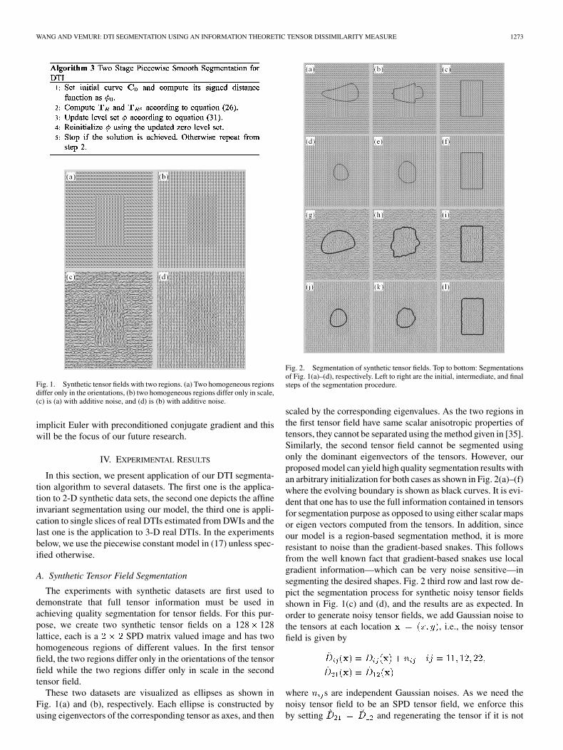
Fig. 1. Synthetic tensor fields with two regions. (a) Two homogeneous regionsdiffer only in the orientations, (b) two homogeneous regions differ only in scale,(c) is (a) with additive noise, and (d) is (b) with additive noise.

implicit Euler with preconditioned conjugate gradient and thiswill be the focus of our future research.

IV. EXPERIMENTAL RESULTS

In this section, we present application of our DTI segmenta-tion algorithm to several datasets. The first one is the applica-tion to 2-D synthetic data sets, the second one depicts the affineinvariant segmentation using our model, the third one is appli-cation to single slices of real DTIs estimated from DWIs and thelast one is the application to 3-D real DTIs. In the experimentsbelow, we use the piecewise constant model in (17) unless spec-ified otherwise.

A. Synthetic Tensor Field Segmentation

The experiments with synthetic datasets are first used todemonstrate that full tensor information must be used inachieving quality segmentation for tensor fields. For this pur-pose, we create two synthetic tensor fields on a 128 128lattice, each is a SPD matrix valued image and has twohomogeneous regions of different values. In the first tensorfield, the two regions differ only in the orientations of the tensorfield while the two regions differ only in scale in the secondtensor field.

These two datasets are visualized as ellipses as shown inFig. 1(a) and (b), respectively. Each ellipse is constructed byusing eigenvectors of the corresponding tensor as axes, and then

Fig. 2. Segmentation of synthetic tensor fields. Top to bottom: Segmentationsof Fig. 1(a)–(d), respectively. Left to right are the initial, intermediate, and finalsteps of the segmentation procedure.

scaled by the corresponding eigenvalues. As the two regions inthe first tensor field have same scalar anisotropic properties oftensors, they cannot be separated using the method given in [35].Similarly, the second tensor field cannot be segmented usingonly the dominant eigenvectors of the tensors. However, ourproposed model can yield high quality segmentation results withan arbitrary initialization for both cases as shown in Fig. 2(a)–(f)where the evolving boundary is shown as black curves. It is evi-dent that one has to use the full information contained in tensorsfor segmentation purpose as opposed to using either scalar mapsor eigen vectors computed from the tensors. In addition, sinceour model is a region-based segmentation method, it is moreresistant to noise than the gradient-based snakes. This followsfrom the well known fact that gradient-based snakes use localgradient information—which can be very noise sensitive—insegmenting the desired shapes. Fig. 2 third row and last row de-pict the segmentation process for synthetic noisy tensor fieldsshown in Fig. 1(c) and (d), and the results are as expected. Inorder to generate noisy tensor fields, we add Gaussian noise tothe tensors at each location , i.e., the noisy tensorfield is given by

where s are independent Gaussian noises. As we need thenoisy tensor field to be an SPD tensor field, we enforce thisby setting and regenerating the tensor if it is not


Fig. 3. Comparison of tensor field segmentation. Top to bottom: Originaltensor field, result using tensor Euclidean distance and result using our newtensor “distance.”

positive definite. This method of generation of the noisy tensorfield is realistic as discussed in Pajevic et al. [24].

B. Affine Invariant Segmentation

When the curve smoothing term in the piecewise constantMumford-Shah model using our tensor “distance” is zero, wehave an affine invariant segmentation model. Using tensordistance based on Frobenius norm, however, does not havesuch a nice property. We now demonstrate an example in Fig. 3to support this statement. Fig. 3(a) shows a tensor field ofsize 128 128, it contains two regions where the region onthe left has vertical orientation while the one on the righthas a horizontal orientation and there is a smooth transitionbetween these two regions. This is an example where thereis no “edge” between two regions and Mumford-Shah basedsegmentation models are particularly effective in such cases.Though there is no agreement on what the groundtruth ishere, we could still assess the performance of segmentationmodels. This is done by checking whether a model can yieldaffine invariant segmentation. Let be the segmentation of theoriginal data, is the transformed segmentation andbe the segmentation of the transformed data. A model is affineinvariant if , when the original data undergoes anaffine transformation.

Fig. 3(b) and (c) shows the transformed tensor fields obtainedby applying two distinct affine transformations to the tensor fieldin Fig. 3(a). The segmentation results using a model based ontensor Euclidean (Frobenius norm based) distance in (17) areshown in Fig. 3(d)–(f). Fig. 3(d) shows the segmentation resultof the original tensor field in (a) where the line in black separatesthe two regions. Fig. 3(e) shows the resulting boundary fromsegmenting the transformed tensor field in (b) in gray while theline in black is the transformed result from Fig. 3(d). Fig. 3(f) is

Fig. 4. A slice of the DTI of a normal rat spinal cord. Top row: viewed channelby channel as gray scale images. Bottom row: viewed using ellipsoids.

similar to Fig. 3(e) except that the transformation is a differentone. We can see there is a big difference between the black lineand the gray line in both Fig. 3(e) and Fig. 3(f) which showsthat using tensor distance based on matrix Frobenius norm inpiecewise constant Mumford-Shah is not affine invariant. Onthe contrary, our proposed method is affine invariant as shownin Fig. 3(g)–(i). The organization of Fig. 3(g)–(i) is the same asthat of Fig. 3(d)–(f). We can see that the gray line coincides withthe black line in (h) and (i) which means that the segmentationis affine invariant. We use so that the curve smoothingterm is negligible in all the above results.

C. Single Slice DTI Segmentation

Fig. 4 shows a slice of the DTI estimated from the DWIsof a normal rat spinal cord where the diffusion tensors in thewhite matter have similar orientations. Each of the six inde-pendent components of the individual symmetric positive defi-nite diffusion tensors in the DTI is shown as a scalar image inthe top row. The arrangements of the components from left toright are— , and . The off diag-onal terms have been greatly enhanced by brightness and con-trast factors for better visualization. An ellipsoid visualizationof same slice as the top row is shown in the bottom row in Fig. 4.Each ellipsoid’s axes correspond to the eigenvector directions ofthe 3 3 diffusion tensor and are scaled by the correspondingeigenvalues. For example, diffusion tensors in free water regionare shown as large round ellipsoids (almost spherical). Fig. 5 de-picts the segmentation process of the gray and white matter in anormal rat spinal cord with the evolving segmentation boundarycurve in black superimposed on the ellipsoid visualization of theDTI.


Fig. 5. Segmentation of the slice of DTI shown in Fig. 4 (a)–(d) are initial,intermediate, and final steps in separating the gray and white matter inside therat spinal cord.

Fig. 6. A slice of the DTI of a normal rat brain. Top row: viewed channel bychannel as gray scale images. Bottom row: viewed using ellipsoids.

Similarly, Fig. 6 shows a slice of DTI of a normal rat brainand Fig. 7 demonstrates the segmentation of the corpus cal-losum using the piecewise constant DTI segmentation model.Though the majority of the corpus callosum is captured in thefinal step, the horns of the corpus callosum are not captured well.This problem is readily remedied by further applying the piece-wise smooth DTI segmentation model [see (15)]. Starting from

Fig. 7. Segmentation of the corpus callosum from a slice of DTI shown inFig. 6 (a)–(d) are initial, intermediate, and final steps of the segmentationprocedure.

Fig. 8. Segmentation of corpus callosum from a the slice of the DTI in Fig. 6using piecewise smooth model. (a) Initial and (b) final steps of the segmentationprocedure.

the segmentation result of the piecewise constant model, piece-wise smooth model achieved a significant refinement as shownin Fig. 8.

D. DTI Segmentation in 3-D

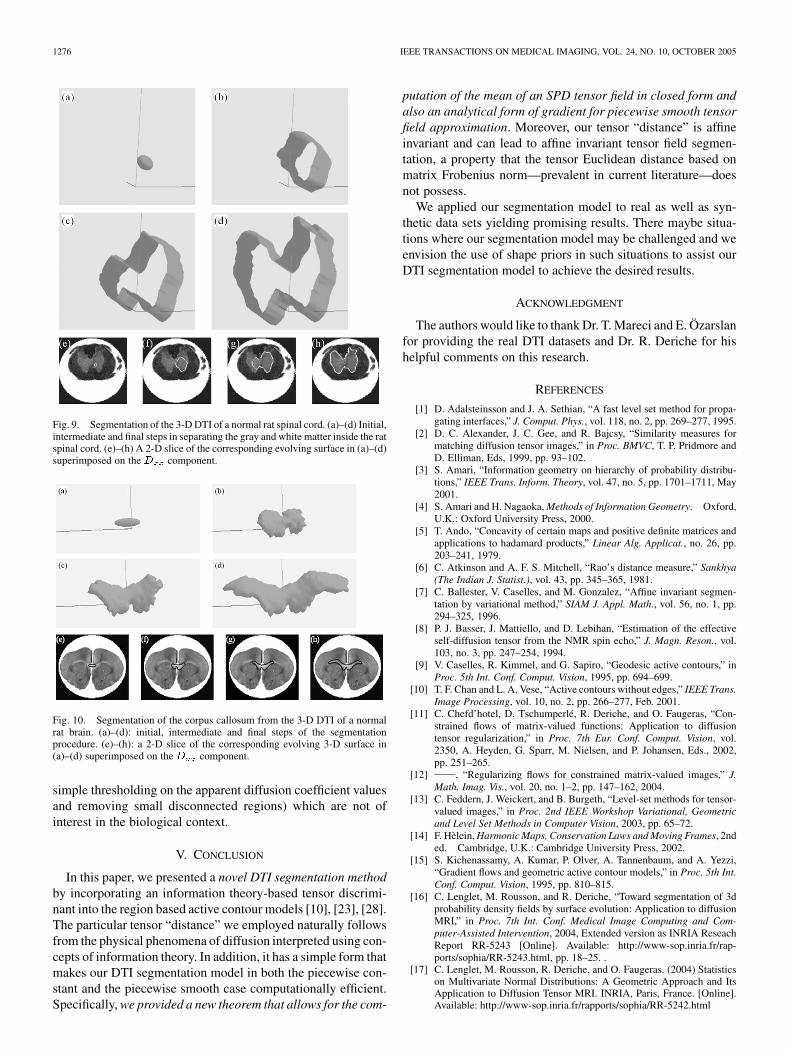
Now we demonstrate segmentation results for two 3-DDTI data sets. Fig. 9 depicts the results of applying the seg-mentation algorithm to a normal rat spinal cord DTI of size108 108 10. Fig. 9(a)–(d) clearly depicts the surface evo-lution in 3-D and Fig. 9(e)–(h) depicts the intersection of thepropagating surface in (a)–(d) with a slice of the compo-nent of the DTI. The separation of the gray and the white matter(where diffusion tensors have similar orientations) inside thenormal rat spinal cord is achieved with ease.

Similarly, Fig. 10(a)–(h) depicts the segmentation proce-dure of the corpus callosum in a normal rat brain DTI of size114 108 12. The effectiveness of our algorithm is againevident, since the dominant part of the corpus callosum is wellseparated from the rest of the volume. Note that in all the realdata experiments, we exclude the free water regions (using


Fig. 9. Segmentation of the 3-D DTI of a normal rat spinal cord. (a)–(d) Initial,intermediate and final steps in separating the gray and white matter inside the ratspinal cord. (e)–(h) A 2-D slice of the corresponding evolving surface in (a)–(d)superimposed on the D component.

Fig. 10. Segmentation of the corpus callosum from the 3-D DTI of a normalrat brain. (a)–(d): initial, intermediate and final steps of the segmentationprocedure. (e)–(h): a 2-D slice of the corresponding evolving 3-D surface in(a)–(d) superimposed on the D component.

simple thresholding on the apparent diffusion coefficient valuesand removing small disconnected regions) which are not ofinterest in the biological context.

V. CONCLUSION

In this paper, we presented a novel DTI segmentation methodby incorporating an information theory-based tensor discrimi-nant into the region based active contour models [10], [23], [28].The particular tensor “distance” we employed naturally followsfrom the physical phenomena of diffusion interpreted using con-cepts of information theory. In addition, it has a simple form thatmakes our DTI segmentation model in both the piecewise con-stant and the piecewise smooth case computationally efficient.Specifically, we provided a new theorem that allows for the com-

putation of the mean of an SPD tensor field in closed form andalso an analytical form of gradient for piecewise smooth tensorfield approximation. Moreover, our tensor “distance” is affineinvariant and can lead to affine invariant tensor field segmen-tation, a property that the tensor Euclidean distance based onmatrix Frobenius norm—prevalent in current literature—doesnot possess.

We applied our segmentation model to real as well as syn-thetic data sets yielding promising results. There maybe situa-tions where our segmentation model may be challenged and weenvision the use of shape priors in such situations to assist ourDTI segmentation model to achieve the desired results.

ACKNOWLEDGMENT

The authors would like to thank Dr. T. Mareci and E. Özarslanfor providing the real DTI datasets and Dr. R. Deriche for hishelpful comments on this research.

REFERENCES

[1] D. Adalsteinsson and J. A. Sethian, “A fast level set method for propa-gating interfaces,” J. Comput. Phys., vol. 118, no. 2, pp. 269–277, 1995.

[2] D. C. Alexander, J. C. Gee, and R. Bajcsy, “Similarity measures formatching diffusion tensor images,” in Proc. BMVC, T. P. Pridmore andD. Elliman, Eds, 1999, pp. 93–102.

[3] S. Amari, “Information geometry on hierarchy of probability distribu-tions,” IEEE Trans. Inform. Theory, vol. 47, no. 5, pp. 1701–1711, May2001.

[4] S. Amari and H. Nagaoka, Methods of Information Geometry. Oxford,U.K.: Oxford University Press, 2000.

[5] T. Ando, “Concavity of certain maps and positive definite matrices andapplications to hadamard products,” Linear Alg. Applicat., no. 26, pp.203–241, 1979.

[6] C. Atkinson and A. F. S. Mitchell, “Rao’s distance measure,” Sankhya(The Indian J. Statist.), vol. 43, pp. 345–365, 1981.

[7] C. Ballester, V. Caselles, and M. Gonzalez, “Affine invariant segmen-tation by variational method,” SIAM J. Appl. Math., vol. 56, no. 1, pp.294–325, 1996.

[8] P. J. Basser, J. Mattiello, and D. Lebihan, “Estimation of the effectiveself-diffusion tensor from the NMR spin echo,” J. Magn. Reson., vol.103, no. 3, pp. 247–254, 1994.

[9] V. Caselles, R. Kimmel, and G. Sapiro, “Geodesic active contours,” inProc. 5th Int. Conf. Comput. Vision, 1995, pp. 694–699.

[10] T. F. Chan and L. A. Vese, “Active contours without edges,” IEEE Trans.Image Processing, vol. 10, no. 2, pp. 266–277, Feb. 2001.

[11] C. Chefd’hotel, D. Tschumperlé, R. Deriche, and O. Faugeras, “Con-strained flows of matrix-valued functions: Application to diffusiontensor regularization,” in Proc. 7th Eur. Conf. Comput. Vision, vol.2350, A. Heyden, G. Sparr, M. Nielsen, and P. Johansen, Eds., 2002,pp. 251–265.

[12] , “Regularizing flows for constrained matrix-valued images,” J.Math. Imag. Vis., vol. 20, no. 1–2, pp. 147–162, 2004.

[13] C. Feddern, J. Weickert, and B. Burgeth, “Level-set methods for tensor-valued images,” in Proc. 2nd IEEE Workshop Variational, Geometricand Level Set Methods in Computer Vision, 2003, pp. 65–72.

[14] F. Hèlein, Harmonic Maps, Conservation Laws and Moving Frames, 2nded. Cambridge, U.K.: Cambridge University Press, 2002.

[15] S. Kichenassamy, A. Kumar, P. Olver, A. Tannenbaum, and A. Yezzi,“Gradient flows and geometric active contour models,” in Proc. 5th Int.Conf. Comput. Vision, 1995, pp. 810–815.

[16] C. Lenglet, M. Rousson, and R. Deriche, “Toward segmentation of 3dprobability density fields by surface evolution: Application to diffusionMRI,” in Proc. 7th Int. Conf. Medical Image Computing and Com-puter-Assisted Intervention, 2004, Extended version as INRIA ReseachReport RR-5243 [Online]. Available: http://www-sop.inria.fr/rap-ports/sophia/RR-5243.html, pp. 18–25. .

[17] C. Lenglet, M. Rousson, R. Deriche, and O. Faugeras. (2004) Statisticson Multivariate Normal Distributions: A Geometric Approach and ItsApplication to Diffusion Tensor MRI. INRIA, Paris, France. [Online].Available: http://www-sop.inria.fr/rapports/sophia/RR-5242.html


[18] R. Malladi, J. A. Sethian, and B. C. Vemuri, “A topology independentshape modeling scheme,” in Proc. SPIE Conf. Geometric Methods inComputer Vision II, vol. 2031, Jul. 1993, pp. 246–256.

[19] , “Evolutionary fronts for topology-independent shape modelingand recovery,” in Proc. 3rd Eur. Conf. Comput. Vision, vol. 800, May1994, pp. 3–13.

[20] , “Shape modeling with front propagation: A level set approach,”IEEE Trans. Pattern Anal. Machine Intell., vol. 17, no. 2, pp. 158–175,Feb. 1995.

[21] , “A fast level set based algorithm for topology-independent shapemodeling,” J. Math. Imag. Vis., vol. 6, no. 2/3, pp. 269–289, 1996.

[22] E. G. Miller and C. Chefd’hotel, “Practical nonparametric density esti-mation on a transformation group for vision,” in IEEE Comp. Soc. Conf.Comput. Vision and Patt. Recog., vol. II, 2003, pp. 114–121.

[23] D. Mumford and J. Shah, “Optimal approximations by piecewisesmooth functions and associated variational-problems,” Comm. PureAppl. Math., vol. 42, no. 5, pp. 577–685, 1989.

[24] S. Pajevic and P. J. Basser, “Parametric and nonparametric statisticalanalysis of DT-MRI data,” J. Magn. Reson., vol. 161, no. 1, pp. 1–14,2003.

[25] M. Rousson, C. Lenglet, and R. Deriche, “Level set and region basedsurface propagation for diffusion tensor MRI segmentation,” in Lec-ture Notes in Computer Science. Berlin, Germany: Springer, 2004, vol.3117, International Workshop Compute Vision Approaches to MedicalImage Analysis (CVAMIA) and Mathematical Methods in BiomedicalImage Analysis (MMBIA), pp. 123–134.

[26] G. A. F. Seber, Linear Regression Analysis. New York: Wiley, 1977.[27] J. A. Sethian, Level Set Methods: Evolving Interfaces in Geometry,

Fluid Mechanics, Computer Vision, and Materials Science. Cam-bridge, U.K.: Cambridge University Press, 1996.

[28] A. Tsai, A. Yezzi, and A. S. Willsky, “Curve evolution implementationof the Mumford-Shah functional for image segmentation, denoising, in-terpolation, and magnification,” IEEE Trans. Image Processing, vol. 10,no. 8, pp. 1169–1186, Aug. 2001.

[29] K. Tsuda, S. Akaho, and K. Asai, “The em algorithm for kernel ma-trix completion with auxiliary data,” J. Machine Learn. Res., vol. 4, pp.67–81, 2003.

[30] Z. Wang and B. C. Vemuri, “An affine invariant tensor dissimilarity mea-sure and its applications to tensor-valued image segmentation,” in IEEEComp. Soc. Conf. Computation Vision and Pattern Recognition, vol. I,2004, pp. 228–233.

[31] , “Tensor field segmentation using region based active contourmodel,” in Lecture Notes in Computer Science, T. Pajdla and J. Matas,Eds. Berlin, Germany, 2004, vol. 3024, Proc. 8th Eur. Conf. Comput.Vision (4), pp. 304–315.

[32] J. Weickert, “Diffusion and regularization methods for tensor-valued im-ages,” presented at the 1st SIAM-EMS Conf. Appl. Math. Our ChangingWorld, Berlin, Germany, Sep. 2001.

[33] M. R. Wiegell, D. S. Tuch, H. W. B. Larson, and V. J. Wedeen, “Auto-matic segmentation of thalamic nuclei from diffusion tensor magneticresonance imaging,” NeuroImage, vol. 19, pp. 391–402, 2003.

[34] S. Yoshizawa and K. Tanabe, “Dual differential geometry associatedwith the Kullback-Leibler information on the Gaussian distributions andits 2-parameter deformations,” SUT J. Math., vol. 35, no. 1, pp. 113–137,1999.

[35] L. Zhukov, K. Museth, D. Breen, R. Whitaker, and A. Barr, “Level setmodeling and segmentation of DT-MRI brain data,” J. Electron. Imag.,vol. 12, no. 1, pp. 125–133, 2003.

IEEE TRANSACTIONS ON MEDICAL IMAGING, VOL. 24, NO. … · DTI Segmentation Using an Information...

Documents

Transcript of IEEE TRANSACTIONS ON MEDICAL IMAGING, VOL. 24, NO. … · DTI Segmentation Using an Information...