IEEE TRANSACTIONS ON KNOWLEDGE AND DATA …ravi/CS260-ST/TKDE-0532-1205-1.pdfIndexing...

Indexing Spatio-Temporal Trajectories withEfficient Polynomial Approximations

Jinfeng Ni and Chinya V. Ravishankar, Senior Member, IEEE

Abstract—Complex queries on trajectory data are increasingly common in applications involving moving objects. MBR or grid-cell

approximations on trajectories perform suboptimally since they do not capture the smoothness and lack of internal area of trajectories.

We describe a parametric space indexing method for historical trajectory data, approximating a sequence of movement functions with

single continuous polynomial. Our approach works well, yielding much finer approximation quality than MBRs. We present the PA-tree,

a parametric index that uses this method, and show through extensive experiments that PA-trees have excellent performance for

offline and online spatio-temporal range queries. Compared to MVR-trees, PA-trees are an order of magnitude faster to construct and

incur I/O cost for spatio-temporal range queries lower by a factor of 2-4. SETI is faster than our method for index construction and

timestamp queries, but incurs twice the I/O cost for time interval queries, which are much more expensive and are the bottleneck in

online processing. Therefore, the PA-tree is an excellent choice for both offline and online processing of historical trajectories.

Index Terms—Access methods, spatio-temporal databases.

Ç

1 INTRODUCTION

GPS is widely used in support of a variety of newapplications, including tracking of vehicle fleets,

navigation of watercraft and aircraft, and the emergencyE911 service for cellular phones [20]. Such applicationswould greatly benefit from an ability to make complexspatio-temporal queries on trajectory data for objectsmoving in two or higher dimensional space.

Current work on indices to support spatio-temporalqueries is typically either in support of predictive queries,which require the future object locations based on theircurrent locations and velocities (“find all objects that will bewithin Union Square in 10 minutes”), or historical queries,which query the past locations of moving objects (“find allobjects which were at Union Square an hour ago”). We focus onhistorical queries, issued on a large set of trajectories.

Queries on historical trajectories may be offline or online[12]. In offline processing, it is generally permissible to havea relatively expensive preprocessing step on the set oftrajectories to optimize query performance [12]. In contrast,online processing assumes that location updates arrive as areal-time data stream so that one must process queries in asthe data is being updated. Online processing is thus a morechallenging task since no preprocessing is possible [5], [12].

We can also classify indexing methods into Native SpaceIndexing methods (NSI) and Parametric Space Indexingmethods (PSI) [26]. In NSI, motion in a d-dimensional spaceis represented as a series of line segments (or curves) indþ 1-dimensional space, using time as an additionaldimension. PSI can be regarded as the dual transformation

of NSI, where a parametric space defined by the motionparameters is used. PSI has been shown to be efficient forpredictive queries (see, for example, TPR-tree [28], TPR*-tree [32], and STRIPES [24]).

PSI has not been advocated in the literature for historicalqueries. Indeed, Porkaew et al. [26] found that NSIoutperformed PSI for historical queries. Predictive trajec-tory uses only one predicted motion function for eachobject, but each historical trajectory may consist ofhundreds or even thousands of motion functions. PSI mayhence incur high storage overhead, significantly degradingquery performance. As a result, much previous work onhistorical queries has used native-space indexing, usingapproximations such as MBRs [13], [12], Octagons [37], orregular grid cells [5].

However, such methods fail to capture some basicproperties of trajectories, which typically consist of a seriesof line segments or curves, with no internal area. As shownby Kollios et al. [14], MBRs are rather coarse approxima-tions for trajectories. Consequently, methods that use MBRs[13], [12] or grid cell approximations [5] either suffer asignificant loss in pruning power or require very expensivepreprocessing.

1.1 Our Work

We revisit the issue of indexing historical trajectories inparametric space for both offline and online processing.Unlike previous work in the area [26], we do not representeach line segment or curve with a parametric function.Instead, we try to approximate a series of line segments orcurves with a single continuous polynomial. This approx-imation may not perfectly match the original trajectory, butwe also keep track of the maximum deviation between theapproximation and the original movement and can stillensure that the approximation is conservative and generatesno false negatives. As long as this maximum deviation issmall, the approximated polynomial function and the

IEEE TRANSACTIONS ON KNOWLEDGE AND DATA ENGINEERING, VOL. 19, NO. 5, MAY 2007 1

. The authors are with the Department of Computer Science andEngineering, University of California, Riverside, 900 University Ave.,Riverside, CA 92521. E-mail: {jni, ravi}@cs.ucr.edu.

Manuscript received 2 Dec. 2005; revised 25 May 2006; accepted 7 Aug. 2006;published online 19 Jan. 2007.For information on obtaining reprints of this article, please send e-mail to:[email protected], and reference IEEECS Log Number TKDE-0532-1205.Digital Object Identifier no. 10.1109/TKDE.2007.1006.

1041-4347/07/$25.00 � 2007 IEEE Published by the IEEE Computer Society

maximum deviation together provide a much tighterapproximation than MBRs and query performance is

significantly improved.We observe first [4] that trajectories tend to be smooth

since objects obey the laws of physics and commonly movealong smooth paths, such as road networks. Indeed, for

similarity-based queries, exploiting the smoothness of

trajectories has improved performance greatly over pre-vious methods [4].

There are major differences between our work and thatof [4], which also approximates trajectories with polyno-

mials. First, [4] targets similarity-based queries and definessimilarity over entire trajectories of equal length, ignoring

the time component. Hence, the techniques in [4] are

generally not applicable to spatio-temporal queries, towhich time is central [25]. Second, the lower-bound lemma

in [4] is only valid for similarity queries so that other

approaches are needed to deal with spatio-temporalqueries. Further, [4] uses approximations of the same

degree for all of the trajectories, which can cause serious

difficulties when the approximation degree is high. Incontrast, we use polynomials of different degrees for

different trajectories.

1.2 Our Contributions

We make a number of contributions in our work. We show

that parametric indexing using polynomial approximationscan improve query performance significantly over current

schemes using native space indexing. We show how to use

polynomial approximations to index historical trajectoriesand how to optimize the degree of the polynomial

approximation.We then present the PA-tree, a new indexing scheme for

historical trajectory data, based on polynomial approxima-tions, and show how to apply PA-trees to support both

offline and online processing of historical trajectories.We also develop an analytical cost model that accurately

predicts query performance using PA-trees. Our model isprospective, relying only on the properties of the trajectories

and the underlying file system. Hence, it can be used to

optimize query performance by tuning parameters. Incontrast, current approaches such as MVR-tree [13], [12]

or SETI [5] must choose parameter values experimentally

since they lack an appropriate cost model.Finally, we evaluate the performance of our schemes

using synthetic trajectory data sets. We show through

extensive experiments that PA-trees have excellent perfor-

mance for offline and online spatio-temporal range queriescompared to current trajectory indexing schemes, such as

MVR-trees and SETI. Compared to MVR-trees, PA-trees are

an order of magnitude faster to construct and incur I/O costfor spatio-temporal range queries lower by a factor of 2-4.

PA-trees underperform SETI for index construction and

timestamp queries, but have half the I/O cost for timeinterval queries, which are much more expensive than

index construction and timestamp queries and are the

bottleneck in online processing. Therefore, the PA-tree is amore appropriate choice for both offline and online

processing of historical trajectories.

2 RELATED WORK

MBRs have been widely used to approximate multi-dimensional data and, consequently, R-trees [10] are themost common index structure for multidimensional data.Earlier work using MBRs for trajectories includes the RT-tree [36] and 3D R-tree [35]. However, since the RT-treedoes not take temporal attributes into account during theinsertion/deletion, timestamp or time interval queries areinefficient. 3D R-tree is inefficient for timestamp queriessince the query time depends on the total number of entriesin the history [31].

Kollios et al. [15] present methods for indexing linearhistorical trajectories offline. They model a long-livedtrajectory with multiple MBRs by splitting it into segmentsto reduce the large dead space resulting from the use of asingle MBR and use partial-persistent R-trees (“PPR-tree”)to index the multiple MBRs. This work is extended in [13],[12], where the motion function could be arbitrary ([12] usesthe term “MVR-tree” in place of “PPR-tree”). This methodcan be more efficient than 3D R-tree since the total emptyvolume after splitting would be reduced. However, sincethis method still uses MBRs for approximating eachsegment, significant dead space remains. Further, they usea global optimization technique to find how to split eachtrajectory into multiple segments, which, unfortunately, isshown to be very time-consuming [27] so that this methodis unsuitable for online applications. To support onlineprocessing, some heuristics are proposed in [12] to speed upthe splitting; however, as their experiments show, asignificant price must be paid in terms of query perfor-mance for this speed-up.

Some previous work has been based on a discrete eventmodel under which an object is assumed to stay at itscurrent position until it issues an update to the server.However, this model cannot be used to represent gradualchanges in object locations, limiting its applicability [5]. Thebasic idea is to build a separate R-tree for each timestamp,as in the HR-tree [21] and the MR-tree [36]. Unchangednodes are not duplicated in consecutive R-trees to reducethe storage cost. However, these index structures are onlyefficient for timestamp queries, but not for time intervalqueries [5], [31]. The MV3R-tree [31] is a hybrid structurethat uses a multiversion R-tree for timestamp queries and asmall 3D R-tree for time-interval queries. The two indicesshare the same leaf pages in order to reduce the storagecost, resulting in a complex algorithm for maintaining theindices [5].

SETI [5] was the first method to consider onlineprocessing of historical trajectories and uses two-tier indexstructures to decouple the spatial and the temporaldimensions. Space is divided into cells and the temporalattributes of all line segments intersecting a cell are indexedwith a one-dimensional index structure. Their resultssuggest that SETI outperforms 3D R-trees and TB-trees[25] for spatio-temporal range queries.

However, several factors diminish query performance inSETI. First, since multiple line segments of the sametrajectory may overlap the query range, SETI must elim-inate duplicates, which may be expensive. Second, grid cellsare rather coarse approximations for trajectories and, hence,

2 IEEE TRANSACTIONS ON KNOWLEDGE AND DATA ENGINEERING, VOL. 19, NO. 5, MAY 2007

a significant I/O cost is incurred in eliminating the false

hits. Third, the work in [5] does not provide a systematic

way to estimate the number of grid cells used in SETI,

which is a key parameter for optimizing the query

performance.Song and Roussopoulos proposed SEB-trees, based on a

zone-based update policy [29]. Their method, like SETI,

divides space into nonoverlapping zones. Within a zone,

objects are indexed in an SEB-tree by their start and end

timestamps. However, as pointed out in [5], this zone-based

update policy does not maintain accurate position informa-

tion within each zone and is unsuitable for supporting

spatio-temporal range queries, which are the focus of our

work.

2.1 Parametric Space Indexing

Another approach is to apply a duality transformation of

movement and index the parameters in parametric space.

Indeed, parametric indexing methods have been shown to

be efficient for predicted trajectories [28], [32], [24].

However, for historical trajectories, [26] shows that para-

metric space index methods were outperformed by native

space index methods. This is due to the fact that, for

predicated trajectories, only one motion function is required

per object, while each historical trajectory may consist of

thousands of motion functions, leading to huge storage

costs if we index all of the motion functions in the index

structure. Unlike [26], we approximate a series of con-

secutive motion functions by a single polynomial function.

Since trajectories are smooth, a low-degree polynomial

suffices to approximate many consecutive motion functions,

with small error. This approach yields a much smaller dead

space than the approximation using MBRs, eventually

leading to improved query performance.Tao et al. [30] use order-k homogeneous recurrence

relations, which they call recursive functions, to represent

predictive trajectories. They approximate each such recursive

function with a polynomial stored at a server and use STP-

trees to index these polynomial coefficients.Several major differences exist between their work and

ours. First, they are concerned with predictive trajectories,

while we focus on historical trajectories. Second, the STP-

tree requires that all trajectories be approximated with

polynomials of the same degree. As acknowledged in [30],

the polynomial degree must trade off the quality of

approximation against the overhead for storage and

manipulation. This trade-off might be different for each

individual trajectory.In contrast, we approximate each individual trajectory

with a polynomial whose degree is tailored to minimize the

expected I/O cost for spatio-temporal range queries and

provide an analytical method for this choice. Further, the

use of a k degree polynomial in [30] for each axis in a

d-dimensional space causes the STP-tree to become an index

structure in a parametric space of ðkþ 1Þd dimensions,

raising the curse of dimensionality for large k. Unlike [30],

we adopt a two-tier structure (see Section 5) to address this

problem.

2.2 Prospective Cost Models

Cost models allow us to understand index structurebehavior and to tune optimization parameters. A numberof analytical cost models [8], [7], [34] have been proposedfor the R-tree [10] and its variants. However, these modelsare applicable only for static spatial objects, but not tospatio-temporal databases with moving objects.

Tao et al. [32] have proposed an approach for modelingthe cost of queries for a given TPR*-tree index. We call suchmodels retrospective since they characterize the behavior of agiven index, using index-specific details such as MBR sizes,available only after a TPR*-tree index is built for any givendata set. In contrast, we seek cost models that are not index-specific and are actually useful in selecting index para-meters. We call such models prospective.

Recently, Tao et al. [33] proposed analytical models foroverlapping and multiversion structures. An overlapstructure, such as OVB-tree [3], or multiversion structures,such as the BTR-tree [16], models attribute changes overtime. However, these analytical models are unlikely to workwell for continuously moving objects. First, the work in [33]assumes a discrete event model under which objectattributes are assumed to be fixed until an update is issued.However, historical trajectory data typically model con-tinuously moving objects. Second, the work in [33] assumesthat all objects remain valid during the lifetime of data set.This assumption is inappropriate for a moving objectdatabase, where a new object will be inserted when it startsto move or an existing object deleted when it stops moving.Consequently, as suggested in [12], current analyticalmodels are unlikely to work well for historical trajectoriesof continuously moving objects when MVR-trees are used.Instead, [12] chooses to tune performance parameters suchas the number of MBRs using nonanalytical approachessuch as volume reduction curves, obtained by runningexperiments with different numbers of MBRs.

Rasetic et al. [27] propose an analytical model foroptimizing the number of MBRs for methods such as [13],[12] when the query size is fixed. Unfortunately, all MBR-based methods must deal with the problems arising from thecoarseness of MBR approximations, and we find that ourmethod far outperforms them. We have found that PA-treesoutperform MVR-trees [13] by a factor of 2-4, even whenthey are given an experimentally optimized number of MBRs.

3 DATA MODEL AND OVERVIEW OF OUR

APPROACH

In many location-based services, location data are obtainedby periodic sampling. Specifically, the trajectory for anobject Oi has the form

TrjðOiÞ ¼ fIDi; t0; t1; � � � ; tn; f0ðtÞ; f1ðtÞ; � � � ; fn�1ðtÞg:

Function fjðtÞ is a movement function representing move-ment during time interval ½tj : tjþ1�, 0 � j � n� 1. Theinterval ½t0 : tn� is the lifetime of the trajectory.

Our approach is applicable to any movement functionfðtÞ as long as we can determine the location of the object atany time instant during its lifetime from fðtÞ. For simplicityof exposition, we adopt a linear mobility model, which is

NI AND RAVISHANKAR: INDEXING SPATIO-TEMPORAL TRAJECTORIES WITH EFFICIENT POLYNOMIAL APPROXIMATIONS 3

widely used in the literature [5], [25]. Each fjðtÞ is now alinear function of time so that a trajectory consists of a seriesof connected line segments, generally called a polyline.

As in previous work [13], [12], we assume time is discreteand that each time instant is an integer in the range ½0; T �,which contains the lifetimes of all the trajectories. Weassume an object moves in a two-dimensional XY-space.The extension to higher dimensions is straightforward.

We focus mainly on spatio-temporal range queries,which are essential building blocks for all other types ofqueries. A spatio-temporal range query may be a timestampquery or a time interval query [13]. A timestamp queryq ¼ ðqs; tÞ asks for all objects within spatial range qs attimestamp t. A time interval query q ¼ ðqs; t1; t2Þ asks for allobjects which were within spatial range qs at any timestampt 2 ½t1 : t2�.

3.1 Overview of Approach

We proceed in two steps. First, we calculate the parametricrepresentation for each trajectory by approximating it inXY-space with two polynomial functions: f̂xðtÞ and f̂yðtÞmodeling movement in the X direction and in theY direction, respectively. We also determine the maximumdeviation of the polynomial approximation from the exactmovement in the X and Y dimensions. The polynomialcoefficients and the maximum deviation suffice for us tomake the approximation conservative, guaranteeing nofalse negatives.

Fig. 1a and Fig. 1b show how we construct linear andorder-k polynomial approximations to the X-component ofa trajectory. Such approximations are not exact, so we createconservative upper and lower bounds for the object’sposition by offsetting the approximating polynomial up-ward and downward by an amount equal to the maximumdeviation between the trajectory and the polynomial. Wecan now guarantee that the object will be located withinthese bounds.

In the second step, we build an index structure over thecoefficients obtained in the first step. However, not alltrajectories are likely to be equally complex so that we mayneed polynomials of different degree for different trajec-tories. This causes problems when building an indexstructure using the coefficients since the dimensionality ofthe indexed items may be different. Current index structuresassume that the dimensionality of all data is the same.Adopting the same polynomial degree for all trajectories isnot advisable since the curse of dimensionality will quickly

degrade the performance of any index structure in high-dimensional space.

3.1.1 Two-Tier Indexing

We address this problem by using a two-tier indexstructure. The first-tier index structure uses only the firsttwo coefficients of each polynomial so that each data entryis a 6-tuple (two coefficients for each dimension and thecorresponding maximum deviations). This strategy ensuresthat we are not operating in a high-dimensional space sothat an R-tree or its variants can still be efficient forindexing. As we will illustrate in Section 4, by appropriatelysplitting the temporal domain ½0; T � into intervals, we canadopt a piecewise linear approximation in the first tierindex structure, each linear approximation correspondingto multiple line segments in the trajectory. However, evenwith this piecewise-linear approximation, we achieve muchsmaller dead space than MBRs can for the same size ofrepresentation.

The second-tier index structure is elaborated within theleaf nodes of the first-tier structure. Complex trajectoriesmay require higher-degree polynomial approximationswhose coefficients are stored in the second-tier structure.If we descend to the leaf nodes in the first-tier structure andstill are unable to determine whether the trajectory satisfiesthe query predicates, the additional coefficients can beretrieved and used in the filtering step. As our experimentswill show, most trajectories can be approximated very wellwith quadratic or cubic polynomials so that the second-tierstructure does not introduce significant space overhead.

3.1.2 An Illustrative Example

Fig. 2a plots the trajectory of a moving vehicle for 10 minutes,collected in the Intellishare project [1] at the University ofCalifornia–Riverside. Fig. 2b plots the X-movement againsttime and the eight MBRs obtained with the LAGreedyalgorithm proposed in [13], [12]. We note that the eightMBRs together require 8� 6 ¼ 48 values. Fig. 2c plots theresult of our method in which the trajectory is split into sixsegments, each approximated with a linear function. Eachsegment requires two coefficients and one maximumdeviation each for X-movement or Y-movement, plus thetemporal intervals. In all, 48 values are required for theapproximations. Our polynomial approximations clearlyproduce much smaller dead space than the MBR approx-imations. Fig. 2d plots the approximation with morecoefficients, with significantly reduced dead space.

4 APPROXIMATING TRAJECTORIES WITH

POLYNOMIALS

In this paper, we propose an approximation in parametricspace by using Chebyshev polynomials. Chebyshev poly-nomials have been shown to have the near-optimalL1 deviation among all approximations with the samedegree [19] and perfectly match our requirements. Further,the Chebyshev coefficients are easy to compute [19], [4].

We have chosen to split each trajectory into multiplesegments by dividing the temporal domain ½0; T � intom disjoint time intervals, each of which is approximatedwith a lower-degree polynomial. There are two reasons for


Fig. 1. Approximating a trajectory segment with polynomials. (a) Linear

approximation. (b) Polynomial approximation.

such splitting. First, approximating the entire trajectory

with a single polynomial may require a polynomial of high

degree, leading to a high-dimensional indexing problem.

Second, the marginal benefit for the first few coefficients

will be much larger than that of high-order coefficients.

4.1 Splitting the Time Domain

We split the temporal domain ½0; T � into m equal time

intervals:

I0 ¼ ½0; lÞ; I1 ¼ ½l; 2lÞ; � � � ;Ii ¼ ½il; ðiþ 1Þl�; � � � ;

Im�1 ¼ ½ðm� 1Þl;mlÞ;

where l ¼ Tm is the length of each time interval and

timestamps l; 2l; � � � ; ðm� 1Þl are called splitting time-

stamps. In Section 8, we will discuss how to optimize m

based on an analytical cost model.Each trajectory is split into multiple segments using the

same m� 1 splitting timestamps. This strategy is different

from that in [13], [12], [27], where each trajectory selects

different splitting timestamps. First, in parametric space, a

set of segments cannot be clustered unless they have the

same temporal domain since it would be meaningless to

cluster coefficients corresponding to different temporal

domains. Second, even with an equal-sized splitting

strategy, we can still use different numbers of coefficients

for different trajectories. Indeed, basing the number of

coefficients for approximation on the trajectory complexity

is equivalent to using different splitting timestamps.

Finally, using equal-length splitting intervals obviates the

need to maintain time intervals in index nodes. This could

significantly reduce the storage cost of the index structure

and eventually lead to a reduction of I/O cost during the

filtering step.

4.2 Approximating a Trajectory Segment with aPolynomial

We now consider how to obtain polynomial approxima-

tion (PA) with Chebyshev polynomials. We illustrate the

approximation for the X-movement only, so we will

omit the subscript x when no confusion can arise.

Consider a trajectory segment in the temporal interval

Ii ¼ ½il; ðiþ 1ÞlÞ. Let fðtÞ be the piecewise linear move-

ment functions during Ii.

We first normalize the temporal domain ½il; ðiþ 1Þl� tothe interval [�1,1]. Given t 2 ½il; ðiþ 1Þl�, let its normalizedvalue be t0 2 ½�1; 1�. Normalization requires

t� ill¼ t

0 � ð�1Þ2

;

which yields

t0 ¼ 2t� ð2iþ 1Þll

and t ¼ ð2iþ 1Þlþ t0l2

:

The function f : ½il; ðiþ 1ÞlÞ ! ð�1;1Þ is now normalizedto ef : ½�1; 1Þ ! ð�1;1Þ.

Now, for t 2 ½il; ðiþ 1Þl�, we can approximate fðtÞ as

bfðtÞ ¼ cð0ÞT0ðt0Þ þ cð1ÞT1ðt0Þ þ � � � þ cðkÞTkðt0Þ; ð1Þ

where t0 2 ½�1; 1� is the normalized value of t, Tiðt0Þ ¼cosði arccosðt0ÞÞ is the Chebyshev polynomial of degree i,and the coefficients cð0Þ; cð1Þ; � � � ; cðkÞ are to be determined.

Theorem 1. Let fðtÞ be the function over interval ½il; ðiþ 1Þl� tobe approximated. Now,

cð0Þ ¼ 1

�

Z 1

�1

efðtÞffiffiffiffiffiffiffiffiffiffiffiffi1� t2p dt; cðiÞ ¼ 2

�

Z 1

�1

efðtÞTiðtÞffiffiffiffiffiffiffiffiffiffiffiffi1� t2p dt:

Proof. See [19]. tu

We use Gauss-Chebyshev quadrature to compute theseintegrals. The abscissas for quadrature are given by theroots of TnðtÞ, which has n roots �j ¼ cos ðj�0:5Þ�

n for1 � j � n. We have the following explicit way to computethe coefficients:

cð0Þ � 1

n

Xnj¼1

fð2iþ 1Þlþ �jl

2

� �;

cðiÞ � 2

n

Xnj¼1

fð2iþ 1Þlþ �jl

2

� �Tið�jÞ:

To ensure that this approximation leads to no falsenegatives, we determine a conservative approximationguaranteed to contain the object’s location at all times.After obtaining the kþ 1 coefficients, we compute themaximum deviation

�ðkÞ ¼ max fðtÞ � bfðtÞ�� n o; t 2 ½il; ðiþ 1Þl�:


Fig. 2. Comparison of approximations for a moving vehicle trajectory. (a) Trajectory of vehicle. (b) MBR approximations. (c) Linear approximation.

(d) Finer approximation.

Now, the range ½bfðtÞ � �ðkÞ; bfðtÞ þ �ðkÞ� is guaranteed tocontain fðtÞ for t 2 ½il; ðiþ 1Þl�.

The kþ 1 Chebyshev coefficients can be computed intime OðnkÞ, where n is the highest degree of approximatingChebyshev polynomial. Computing the maximum devia-tion error takes time OðlkÞ, where l is the number of instantsbetween t0; ts. In our implementation, we choose n ¼ OðlÞ,so the total cost is OðlkÞ. The following lemma is useful:

Lemma. Suppose fðtÞ is approximated by a linear functionbfðtÞ ¼ cð0Þ þ cð1ÞT1ðt0Þ. For il � t1 < t2 � ðiþ 1Þl, we havejbfðt2Þ � bfðt1Þj ¼ 2ðcð1Þjt2 � t1jÞ=l.

Proof.

jbfðt2Þ � bfðt1Þj ¼ jðcð0Þ þ cð1Þt02Þ � ðcð0Þ þ cð1Þt01Þj¼ 2cð1Þjt2 � t1j

l:

tu

4.3 Choosing the Degree of ApproximatingPolynomials

In general, the polynomial degree k should be determinedbased on the characteristics of trajectories. Clearly, there is atrade-off between the approximation quality and thedegree k used for approximation. A smaller k value requiresless space in the index, as well as less I/O during the filterstep. On the other hand, fewer coefficients may result inpoorer filtering, causing more trajectories to be examinedduring the refinement step, increasing its I/O cost.

Another consideration is the complexity of the trajectorysegment. Obviously, if the trajectory segment has arelatively simple form, a few coefficients will suffice to geta small deviation error. However, since we are not aware ofany well-defined notion of complexity for this context, it isnot easy to estimate the optimal degree.

We present a heuristic to estimate the degree k, aimed atminimizing the expected size of representations to beretrieved during query evaluation. Let �ðkÞx and �ðkÞy be themaximum errors for a k-order polynomial approximationon the X- and Y-dimensions, respectively. We make thefollowing reasonable assumptions: First, given queryq ¼ ðqs; t1; t2Þ, we assume that the query range qs is a qx �qy rectangle, where qx � 2�ðkÞx and qy � 2�ðkÞy . (The other casesare similar and, hence, omitted). Second, we assume thatthe range qs is uniformly distributed in the region normal-ized to a unit square.

Let S and Sk be the data sizes of the exact representationsfor the trajectory segment and of its k-degree polynomialapproximation, respectively. We will derive the expectedsize of representational data to be retrieved for a randomquery.

If the approximation does not intersect the query range,we can safely prune it out during the filter step. If asegment’s approximation lies completely inside qs, we cansafely declare it a true hit. We call this type of true hit afiltering true hit. Otherwise, the segment becomes a candidatefor the refinement step in which its exact representationmust be retrieved. If the refinement step finds that thesegment lies outside qs, we have a false hit. Otherwise, wewill record a refinement true hit.

4.3.1 Estimating Relevant Probabilities

To estimate the expected I/O cost, we must estimate theprobability that the trajectory segment is a candidate for therefinement step in which it will be determined to be either afalse hit or a refinement true hit. We will consider the hitsand misses on the X and Y dimensions separately, omittingthe x and y subscripts and the subscript k when noconfusion is likely.

We first define a class of events to help our development(see Table 1). Consider a segment s, an approximation bs fors, and a query range qs ¼ qx � qy. Let the projections of bsalong the X- and Y- axes be bsx and bsy, respectively.

We have an X-raw hit (or just X-hit) if bsx intersects qxduring the filtering step. We will denote this event as HXðsÞ.Further processing is required for us to determine whetherthis hit is a true hit or a false hit. If bsx lies entirely within thequery range qx, we can flag this as a filtering true hit anddispense with the refinement step. We denote this event byfTHXðsÞ. If we have HXðsÞ but not fTHXðsÞ, we pass s to therefinement step for further processing. In this case, we willdesignate s as an X-candidate and write CXðsÞ.

Let the query range qs’s X-projection be ½u� qx; u�. Let! be the overlap between the lifetime of s and the querytemporal interval ½t1; t2�, with j!j being the length of thisoverlap. Let bfmin and bfmax be the minimum andmaximum value of the approximated polynomial bfxðtÞwithin !. As seen in Fig. 3, if u 2 ½bfmin � �ðkÞx ; bfmin þ �ðkÞx � oru� qx 2 ½bfmax � �ðkÞx ; bfmax þ �ðkÞx �, the trajectory segment is acandidate for the refinement step. In this case, althoughthe projection bsx of bs overlaps ½u� qx; u�, it is still unclearwhether s itself intersects with qs along the X-dimension.Hence, the probability that the trajectory segment is anX-candidate is

Pr½CX� ¼ 2�ðkÞx þ 2�ðkÞx ¼ 4�ðkÞx : ð2Þ

To estimate the probability that the trajectory segment is an

X-hit, we observe that, during !, the projected approximated


TABLE 1Summary of Notation for Events

Fig. 3. X-candidate example.

movement along the X-dimension is bfmax � bfmin, associated

with approximation error 2�ðkÞx . We know from Lemma 1

that, when a linear function bfxðtÞ is used to approximate the

X-movement, bfmax � bfmin ¼ 2 cð1Þx j!jl , where l is the length of

the temporal interval. Now, the probability that the

trajectory segment is an X-hit is

Pr½HX� ¼ 2�ðkÞx þ 2cð1Þx j!jlþ qx:

If the approximation bsy does not result in a Y-hit, we can

safely prune out the segment. However, when a trajectorysegment is an X-candidate and a Y-Hit, it remains unclearduring the filter step whether the trajectory segment

satisfies the query predicate, so the segment becomes arefinement candidate. A symmetric situation holds when

the segment is a Y-candidate and an X-intersect. Therefore,the probability of becoming a refinement candidate is

Pr½C� ¼ Pr½ðCX \HYÞ [ ðCY \HXÞ�¼ Pr½CX� � Pr½HY� þ Pr½CY� � Pr½HX� � Pr½CX� � Pr½CY�

since CX HX and CY HY. Equation (2) and symmetry

between CX and CY yields

Pr½C� ¼ 4 �ðkÞx � qy þ �ðkÞy � qx� �

þ 8j!jl

�ðkÞx � cð1Þy þ �ðkÞy � cð1Þx� �

:

Now, the expected I/O cost for the trajectory segment swith a degree-k approximation is

IOk ¼ Sk þ Pr½C�S;

where S and Sk are the data sizes of the exact representa-tions for s and of its degree-k polynomial approximation,respectively. We will choose k to minimize IOk.

5 PA-TREES

We now present the PA-tree, a new method for indexingpolynomial approximations of 2D trajectories. PA-trees

resemble R*-trees, but each entry consists of polynomialcoefficients, rather than MBRs. We recall that the temporal

domain ½0; T � is split into m intervals. In a gross sense, theroot node has m PA-trees as its children, each responsible

for indexing trajectory segments within one of theseintervals.

Fig. 4a shows two PA-trees, over intervals I1 and I2,respectively. Indexing occurs at two tiers. The first tier ofindexing is an R*-tree like structure, and indexes the twoleading coefficients of the polynomial describing move-ment along each dimension. It is reasonable to see this asa four-dimensional indexing problem, with each dimen-sion corresponding to one coefficient. Each entry in theindex structure also holds the maximum deviation errors�ð1Þx and �ð1Þy .

As in R*-trees, a leaf node entry has the form ðptr; paÞ,where ptr points to the exact representation of the trajectory

segment and pa is a 6-tuple: hcð0Þx ; cð1Þx ; cð0Þy ; cð1Þy ; �ð1Þx ; �ð1Þy i.Entries in nonleaf nodes are of the form ðptr; paÞ, where

ptr is the pointer to a child node and pa has the form

hcð0Þ?;x; cð0Þ?;y; c

ð1Þ?;x; c

ð1Þ?;y; c

ð0Þ>;x; c

ð0Þ>;y; c

ð1Þ>;x; c

ð1Þ>;y; �

ð1Þx ; �ð1Þy i, representing

the lower (upper) bounds of the coefficients for the entries

stored in the child pointed to by ptr. Also, pa maintains the

maximum �ð1Þx and �ð1Þy for all entries in the subtree.The second tier holds more coefficients and the max-

imum deviation for each trajectory segment, if the estimateddegree is larger than 1 (See Section 4). This informationallows better pruning than the linear approximations in thefirst tier.

Insertions and deletions are similar to the corresponding

operations for R*-tree. The primary difference is that we

need to ensure that the �ð1Þx , �ð1Þy values in the nonleaf nodes

are the maximum �ð1Þx , �ð1Þy for all the segments in its subtree.Fig. 4b depicts a set of PA-trees, showing only the

coefficients and deviations for X-dimension for simplicity.The root entries specify the time interval for each individualPA-tree. Each first-tier entry contains the lower and upperbounds for the coefficient cð0Þ and cð1Þ, as well as themaximum deviation error �ð1Þ. Each entry in the second tierhas the form of k; cð2Þ; � � � ; cðkÞ; �ðkÞ; ts; te.

6 OFFLINE QUERY PROCESSING

Given a query q ¼ ðqs; t1; t2Þ, we start with the root node,which contains m temporal intervals and the pointers to thecorresponding PA-tree. Each PA-tree is searched if and onlyif the temporal interval intersects ½t1; t2�.


Fig. 4. (a) PA-tree and (b) an example.

Let Ii ¼ ½il; ðiþ 1Þl� be the temporal interval correspond-

ing to an entry in a nonleaf node in the PA-tree. Given

q ¼ ðqs; t1; t2Þ, let ts ¼ maxft1; ilg and te ¼ minft2; ðiþ 1Þlg.We must check whether there is a trajectory segment

inside qs at any time t 2 ½ts; te�. Let the index entry be

hcð0Þ?;x; cð0Þ?;y; c

ð1Þ?;x; c

ð1Þ?;y; c

ð0Þ>;x; c

ð0Þ>;y; c

ð1Þ>;x; c

ð1Þ>;y; �

ð1Þx ; �ð1Þy i. In the fol-

lowing discussion, we will omit the subscripts x and y

for the sake of clarity.

As in Section 4, for t 2 ½ts; te�, we use t0 to denote its

normalized value in [�1; 1]. Now, the nonleaf entry

represents all movement in the approximated linear form

f 0ðtÞ ¼ cð0Þ þ cð1ÞT1ðt0Þ ¼ cð0Þ þ cð1Þt0, where cð0Þ 2 ½cð0Þ? ; cð0Þ> �

and cð1Þ 2 ½cð1Þ? ; cð1Þ> �. In principle, we can apply the dual

transformation technique of [14] to check whether there

are linear trajectories intersecting qs during ½t0s; t0e�. How-

ever, the slope cð1Þ and the temporal attribute t0 could be

either positive or negative, making it hard to apply duality

transformations. Instead, we determine the upper and

lower bounding polynomials for the motion segment in

the form cð0Þ þ cð1Þt, where cð0Þ 2 ½cð0Þ? ; cð0Þ> �, cð1Þ 2 ½c

ð1Þ? ; c

ð1Þ> �,

and t0 2 ½t0s; t0e�. If eð1Þ is the maximum deviation error, we

use the monotonicity of cð0Þ þ cð1Þt0 to compute the lower

bound as:

x? ¼ cð0Þ? þminfcð1Þ? t0s; cð1Þ? t0e; c

ð1Þ> t0s; c

ð1Þ> t0eg � �ð1Þ ð3Þ

and the upper bound as:

x> ¼ cð0Þ> þmaxfcð1Þ? t0s; cð1Þ? t0e; c

ð1Þ> t0s; c

ð1Þ> t0eg þ �ð1Þ: ð4Þ

If the computed range intersects with the query range qs,

we know there may be candidates satisfying the query

predicates. We now descend the tree and repeat the process

for the subtree rooted at this entry, down to the leaf nodes.

At the leaf node, we first retrieve the k� 1 coefficients

in the second-tier structure, stored sequentially in the leaf

nodes. The approximate location bfðtÞ at time t 2 ½ts; te�can be computed using (1) and the spatial range

½bfðtÞ � �ðkÞ; bfðtÞ þ �ðkÞ�. If there is a time t 2 ½ts; te� such

that the spatial range is completely inside qs, the

trajectory segment is a filtering true hit, its ID will be

reported. If this range does not intersect query qs for any

t 2 ½ts; te�, the trajectory segment is pruned out. Other-

wise, refinement is required for determining whether this

trajectory segment is a true hit or false hit.

6.1 An Example

Consider the PA-trees shown in Fig. 4b. Let the query have

spatial range qx ¼ ½0; 0:1� in the X-dimension and temporal

interval [10, 20]. Clearly, the PA-trees corresponding to the

interval [0, 20] and the one for [20, 40] must both be

searched. Normalizing the query interval to [0, 1], we can

use (3) and (4) and obtain [0, 0.4] as the range for entry 1.

Since qx overlaps this range, we need to check entries 2 and

3, which are entry 1’s children. For entry 2, we use (3) and

(4) and get the range as [0.15, 0.35], which does not intersect

with qx ¼ ½0; 0:1�. We can safely prune out this entry. For

entry 3, we get the range as [0, 0.4], which overlaps qx.

We now retrieve entry 5 in the second-tier structure.

For this trajectory segment, we have k ¼ 2, cð0Þ ¼ 0:3,

cð1Þ ¼ �0:2, cð2Þ ¼ 0:25, and �ð2Þ ¼ 0:03. For each timestamp

t 2 ½10; 20�, we calculate bfðtÞ using (1). For t ¼ 10, we

calculate the value of bfðtÞ to be 0.05. We now compute

the range to be ½bfðtÞ � �ð2Þ; bfðtÞ þ �ð2Þ� ¼ ½0:02; 0:08�, which

is completely inside qx ¼ ½0; 0:1�. Therefore, we identify

this trajectory segment as a true hit.

7 ONLINE PROCESSING

We now extend PA-trees to support online processing when

location updates arrive as real-time data streams. We

support both efficient index structure maintenance and

query.

7.1 Handling Inserts

Fig. 5 shows the insert procedure in our online scheme. As

in the offline case, we split the lifetime into intervals of

length l. Let Inow ¼ ½il; ðiþ 1ÞlÞ be the current interval and

let tnow be the current time, il � tnow � ðiþ 1Þl. As in [5],

updates arriving during ½il; iþ 1ÞlÞ will be stored in an in-

memory buffer, called the frontline buffer. At the end of the

current interval, that is, at tnow ¼ ðiþ 1Þl, we obtain

polynomial coefficients and deviation errors, as in Section 4.

These values are then inserted into a PA-tree and the

trajectory data placed in a data file.

7.1.1 Buffer Management

One major concern is that the frontline buffer may overflow

before the end of the interval, especially for relatively long

intervals or when updates arrive rapidly. We use the

technique of batch writes, as in [17]. When the buffer is full,

its contents are written to an intermediate list as a single

batch. Similarly, at the end of an interval, an intermediated

list is retrieved as a batch and the polynomial approxima-

tion applied over the entire trajectory segment correspond-

ing to this interval. Since reading and writing each

intermediate list requires one random access followed by

a long sequential read [17], the I/O overhead is greatly

reduced.


Fig. 5. Insert procedure.

7.2 Handling Queries

Consider a time interval query q ¼ ðqs; t1; t2Þ. Let Inow be thecurrent interval and tnow be the current time. To process q,we must first determine the temporal intervals up to Inowthat overlap ½t1; t2�. If Inow itself overlaps ½t1; t2�, we firstcheck whether the trajectory segment in the frontline bufferoverlaps qs during ½t1; t2�. The trajectory segments in theintermediate lists will next be retrieved and tested against q.All trajectory segments from temporal intervals I thatprecede Inow and overlap ½t1; t2� will have already beenindexed in a PA-tree. Therefore, the query processingtechnique presented in Section 5 suffices to find all of thetrajectory segments that intersect qs during interval I.

8 A PROSPECTIVE PERFORMANCE MODEL

We now develop an analytical cost model for PA-trees. Inthe terminology of Section 2, we seek cost models that areprospective, rather than retrospective. That is, we seek modelsuseful in designing PA-tree structures for a given data setand in tuning important index parameters, such as thenumber of temporal intervals, to minimize the number ofdisk accesses.

We are given N trajectories during the lifetime ½0; T �in a two-dimensional unit square and a time intervalquery q ¼ ðqs; t1; t2Þ. We want a formula to estimate theaverage number of disk access for processing q duringthe filtering and refinement steps. As in Section 4, wedivide the lifetime ½0; T � into m equal-sized intervals½0; lÞ; ½l; 2lÞ; � � � ; ½ðm� 1Þl;ml�, where l ¼ T=m is the timeinterval length. Let the PA-tree corresponding to theith interval be denoted by PAi.

We make the following reasonable assumptions: First,

the query spatial range qs ¼ qx � qy is uniformly distributed

in the unit square and the query temporal interval ½t1; t2� is

uniformly distributed within ½0; T �. Second, for trajectory

segment s, we assume that we know the coefficients cð1Þs;x and

cð1Þs;y , the linear deviation errors �ð1Þs;x and �ð1Þs;y , and the k-order

approximation errors �ðkÞs;x and �ðkÞs;y . These values can be

obtained using the polynomial approximation technique

discussed in Section 4. Finally, we assume that there is no

buffering since our purpose is to model the PA-tree without

the confounding effects of a buffer management algorithm.

Let Ni be the number of trajectory segments indexed byPAi and hi be the height of PAi. Let f be the fanout of nodein PAi, that is, the average number of entries in a node. LetMi;j be the number of nodes at level j. Leaf nodes are atlevel 1, root node is at level h, and the data entries are atlevel 0. Now, as in the R-tree cost model of [34], we have:

hi ¼ logf Ni and Mi;j ¼Ni

fj: ð5Þ

Let DAfi ðqÞ be the the number of disk access for PAi

during the filtering step for query q. Let DAri ðqÞ be the

number of disk accesses to the trajectory segments for theith interval during the refinement step. The total number ofdisk access would be

DAðqÞ ¼Xmi¼1

�DAf

i ðqÞ þDAri ðqÞ

: ð6Þ

8.1 Cost Model for Filtering Step

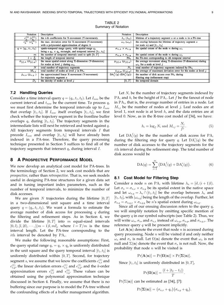
Consider a node n on PAi with lifetime �n ¼ ½il; ðiþ 1ÞlÞ.Let �n ¼ �n;x � �n;y be its spatial extent in the native spaceand let !n;q ¼ �n \ ½t1; t2� be the overlap between �n and½t1; t2�, with j!n;qj being the length of the overlap. Further, let�n;q ¼ �n;q;x � �n;q;y be n’s spatial extent during !n;q.

Since all of our ensuing discussion refers to the query q,we will simplify notation by omitting specific mention ofthe query q in our symbol subscripts (see Table 2). Thus, wewill write !n, �n, and �n;x instead of !n;q, �n;q, and �n;q;x. Thereference query q will be present implicitly.

Let AðnÞ denote the event that node n is accessed duringquery processing. Node n will be visited if and only neither!n and �n is null. Let �ðnÞ denote the event that !n is notnull and �ðnÞ denote the event that �n is not null. Now, theprobability that node n will be visited is

Pr½AðnÞ� ¼ Pr½�ðnÞ� � Pr½�ðnÞ�:

Since ½t1; t2� is uniformly distributed in ½0; T �,

Pr½�ðnÞ� ¼ ðlþ jt2 � t1jÞT

:

Pr½�ðnÞ� can be estimated as [34], [7]:

Pr½�ðnÞ� ¼��n;x þ qx

��n;y þ qy

:


TABLE 2Summary of Notation

As in our discussion of query processing in Section 6, we

compute each node’s spatial extent as the sum of a

component derived from the approximated object move-

ment and a component corresponding to the maximum

deviation error of the linear approximation. Given

Mi;j nodes at level j in PA-tree PAi, let the mean spatial

extents along the X-dimension and Y-dimension for the

nodes at level j during !n be ��½j�;x ¼ 1Mi;j

PMi;j

m¼1 �m;x and

��½j�;y ¼ 1Mi;j

PMi;j

m¼1 �m;y, respectively. Let ��½j�;x and ��½j�;y be the

average movement of objects at level j along the X- and Y-

dimensions during !n, derived from the trajectory approx-

imations. Let ��½j�;x and ��½j�;y be the average of the maximum

deviation errors of the nodes at level j. The average spatial

extent of a level-j node is

�½j�;x ¼ �½j�;x þ 2�½j�x; and �½j�;y ¼ �½j�;y þ 2�½j�y: ð7Þ

We will now discuss how to estimate ��½j�;x (or ��½j�;y) and��½j�;x (or ��½j�;y).

8.1.1 Estimating Object Movements

Each node in the PA-tree maintains the coefficients for thelinear approximation to the trajectories. We estimate ��½j�;xand ��½j�;y as follows: We use the linear approximation foreach segment s to compute a time-parameterized MBR during!s, the overlap between s’s lifetime and query temporalinterval ½t1; t2�. A time-parameterized MBR for a trajectorysegment is the MBR, which covers the approximated linearmovement during !s, and can easily be obtained from theparametric representations of PA-tree. During the temporalinterval !s, the PA-tree may be regarded as a time-parameterized R-tree over those MBRs in the native space.Under this formulation, we can apply the cost model forgeneral R-tree [34] to estimate the spatial extent ��½j�;x � ��½j�;yin the PA-tree.

From Lemma 1, the approximated linear X- and Y-movements for trajectory segment s during !s are

�̂s;x ¼2cð1Þs;x � j!sj

land �̂s;y ¼

2cð1Þs;y � j!sjl

;

where cð1Þs;x and cð1Þs;y are the linear coefficients for s and j!sj isthe length of overlap !s.

Therefore, in the native space, the trajectory segment willbe approximated by a time-parameterized MBR with area

as ¼ �̂s;x � �̂s;y ¼ 4cð1Þs;x � cð1Þs;y � j!sj

2

l2:

To use the R-tree [34] cost model in our analysis, we must

estimate the density Dj for the set of time-parameterized

MBRs of nodes at level j during !n. As in [34], the density of a

set of MBRs is simply the total size of MBRs when the entire

space is an unit square. In our case, the density D0 at level 0

would be the total size of all time-parameterized MBRs

during !s for all trajectory segment s ð1 � s � NiÞ. That is,

D0 ¼XNi

s¼1

as ¼XNi

s¼1

4cð1Þs;x � cð1Þs;y � j!sj

2

l2¼ 4

l2

XNi

s¼1

j!sj2cð1Þs;xcð1Þs;y : ð8Þ

As in [34], the density Dj ð1 � j � hiÞ at level j becomes:

Dj ¼ 1þffiffiffiffiffiffiffiffiffiffiDj�1

p� 1ffiffiffi

fp

!2

:

Now, ��½j�;x and ��½j�;y can be computed as follows:

�½j�;x ¼ �½j�;y ¼ffiffiffiffiffiffiffiffiffiDj

Mi;j

s¼

ffiffiffiffiffiffiffiffiffiffiDjfj

Ni

s:

8.1.2 Estimation of Deviation Errors

To estimate the average of maximum deviation error ��½j�;x or

��½j�;y for the nodes at level j, we observe that the deviation

error is an augmented attribute in PA-trees and does not

affect the node insert/split procedure when constructing

PA-trees. The deviation errors are hence independent of the

polynomial coefficients and we proceed to estimate devia-

tion error as follows:The deviation errors �ð1Þs;x or �ð1Þs;y for trajectory segments

s ð1 � s � NiÞ are randomly assigned into Mi;j buckets.

Then, we use the average of the maximum deviation error

of the Mi;j buckets as the estimation of ��½j�;x and ��½j�;y.

8.1.3 Total Cost for Filtering Step

Using our estimates of ��½j�;x or ��½j�;y and ��½j�;x or ��½j�;y, we can

now compute the average spatial extent ��½j�;x and ��½j�;y of the

node at level j using (7). The total number of disk accesses

DAfi ðqÞ over the PAi is:

DAfi ðqÞ ¼

ðlþ jt2 � t1jÞT

Xhij¼1

Mi;jð�½j�;x þ qxÞð�½j�;y þ qyÞ�

¼ ðlþ jt2 � t1jÞT

Xhij¼1

Ni

fjð�½j�;x þ qxÞð�½j�;y þ qyÞ

� �:

8.2 Cost Model for Refinement Step

Given a trajectory segment s, let �s denote its temporal

interval. Let �ðsÞ be the event that �s overlaps with the

query temporal interval ½t1; t2�. As in the analysis of the

filtering step, we have

Pr½�ðsÞ� ¼ j�sj þ jt2 � t1jT

:

Let CðsÞ be the event that trajectory segment s is a

candidate segment for refinement step. As discussed in

Section 4,

Pr½CðsÞ� ¼ 4ð�ðkÞs;x � qy þ �ðkÞs;y � qxÞ þ 8j!sjl

ð�ðkÞs;y � cð1Þs;x þ �ðkÞs;x � cð1Þs;yÞ:

Therefore, the total number of disk access over PAi

during the refinement step is

DAri ðqÞ ¼

XNi

s¼1

Pr½�ðsÞ�Pr½CðsÞ� ¼ 4

T

XNi

s¼1

ðj�sj þ jt2 � t1jÞ

��ðkÞs;x � qy þ �ðkÞs;y � qx þ 2

j!sjlð�ðkÞs;x � cð1Þs;y þ �ðkÞs;y � cð1Þs;xÞ

:


8.3 Analytical Method for Parameter Tuning

One application of the cost model is for tuning theparameter m for a PA-tree. Let DAmðqÞ be the expectationof the total I/O cost when we use m intervals. To estimatethe optimal or near-optimal value for m, we estimateDAmðqÞ using the cost model, varying parameter m, andthen choose the optimal value m̂opt as the value of m whenDAmðqÞ is minimal.

Another approach to parameter tuning, which we havecalled the experimental method, was used in [12], [5]. Thisapproach first constructs a set of index structure instances,one for each value of the parameter. It then evaluates a set ofqueries over each of these index instances and picks as theoptimum the instance that yields the lowest cost. In Section 9,we will show that the analytical method for parametertuning is far cheaper than the experimental method whileyielding a near-optimal value for parameter m.

9 EXPERIMENTAL EVALUATION

Since no large-scale real trajectory data sets are currentlyavailable publicly, we generated synthetic data sets using thenetwork-based generator of [2] and the road network in SanJoaquin County, California. Our data sets were obtained byrunning the simulation for a total of 1,000 timestamps. Wefocus on the results on the data sets generated by thisgenerator, which has been used extensively in previous work[5], [12], [37]. Further, as suggested by recent work [23], [9],modeling movement along roads is practically significant.

Data set SJ30k was generated by repeating the followingprocedure six times, each with different random seeds. Fivethousand trajectories were generated each time, using sixobject classes, three external object classes, 3,000 initialobjects, and two new objects per timestamp. This data sethas 6,390,000 location updates and a size of 180 MB. Eachobject reports its position and movement function each timeinstant during its lifetime, so the number of movementfunctions for each object equals the number of instants in itslifetime.

We compared the PA-tree with the MVR-tree [13], [12]and SETI [5] for offline processing and with SETI for onlineprocessing. The MVR-tree is shown to be an efficientapproach for offline processing, outperforming the 3DR-tree approach or piecewise R-tree (pw-Rtree) [12], whileSETI is the first approach to support efficient onlineprocessing.

We implemented the PA-tree and SETI1 with the SpatialIndex Library of [11]. We used the MVR-tree implementa-tion in [12], which uses the LAGreedy algorithm to modeleach trajectory with multiple MBRs. In the followingfigures, the legend PA represents our method, MVR

represents the method of [13], [12], while SETI representsthe method of [5].

9.1 Setup

Our experiments were run on an Intel Pentium IV 1.7 Ghzprocessor, with 512 Mbytes of main memory. We choosepage size of 4 Kbyte in all experiments. Unlike [5], which

used a fixed size buffer even larger than the data size insome cases, we use a buffer with size being about 10 percentof the original data set, as suggested by Mamoulis andPapadias [18]. Unlike [12], we do not reset the buffer beforeexecuting every query since resetting the buffer will renderthe buffer useless when evaluating a workload of multiplequeries. Further, as in [6], we assume the ratio of cost ofsequential I/O to that of random I/O is 1:20 and charge10ms for each random I/O.

We evaluated performance with respect to index struc-ture size, varying the number of MBRs for the MVR-tree, thenumber of intervals for the PA-tree, and the number of gridcells for SETI. Let there be N trajectories and let the MVR-tree use ð1þ SÞN MBRs. We varied S from 10 to 3,000. Forthe PA-tree, we varied m, the number of intervals that thetemporal domain is split into, from 5 to 200. For SETI, wevaried the number C of cells from 25 to 3,600.

We used various types of query workloads, eachcontaining 1,000 queries, and varied qt ¼ jt2 � t1j, the lengthof the temporal interval, and the size of query spatial range.We chose qt ¼ 1 for timestamp queries, and qt ¼ 50 and qt ¼100 for medium and large time interval queries, respec-tively. As in [33], [5], each query’s spatial range was asquare uniformly distributed in the unit square, with theedge length ql ¼ qx ¼ qy being 5 percent, 7 percent, or 10percent. The following figures report the average perfor-mance for each query. Table 3 shows the setup for ourexperiments.

9.2 Comparing Approximation Quality

To gauge the potential for improvement with our scheme,we compare the dead space using our method with thatusing the MBR approximation obtained from the LAGreedyalgorithm [13]. This metric captures the pruning power ofindex structures based on the respective approximations.Larger amounts of dead space would suggest smallerpruning power since it will result in more refinementcandidates.

The volume of each MBR is simply the product of theedge lengths along the X-dimension, Y-dimension, and thetemporal dimension. Each entry is a 6-tuple, as discussed inSection 3. If we use kþ 1 coefficients each to approximatethe X-movements and Y-movements, the volume of deadspace can be computed as 4�ðkÞx �ðkÞy ðts � t0Þ, where ½t0; ts� isthe temporal domain. The representation size is 2ðkþ 1Þ þ 5since we represent 2ðkþ 1Þ coefficients in all, the value of k,as well as the maximum deviation and the temporaldomain.


1. We reimplemented SETI since the original source code was notavailable.

TABLE 3Experimental Parameters

Figs. 6a and 6b compare the quality of our method withthat of MBR approximations for 5,000 trajectories wheneach coefficient, deviation error, coordinate, or k takes up4 bytes. For a given representation size, our method hasdead space up to 2-5 times smaller than that for MBRapproximations, showing clear potential for improvingquery performance.

9.3 Accuracy of Cost Model

To demonstrate the accuracy of our analytical model, wecompared the I/O cost estimated from the cost modelagainst the I/O obtained from experiments. As explained inSection 8, we do not use buffers in this set of experiments.Figs. 7a, 7b, and 7c plot the average I/O cost against thenumber m of intervals, when ql is 5 percent, 7 percent, and10 percent, respectively. Clearly, our estimated I/O costmatches the experimental I/O cost very closely, withrelative error no more than 25 percent. Furthermore, theestimated query cost captures quite closely the trade-offbetween m and the query performance, as we will discussin Section 9.4.1.

Our ability to capture this trade-off enables us to obtain anear-optimal value for the number of intervals. Table 4shows the excellent match between the value m̂opt obtainedfrom our cost model and the optimal value mopt obtainedfrom experiments. Figs. 7d, 7e, and 7f compare the I/O costwhen m ¼ mopt with the I/O cost when m ¼ m̂opt. To seehow much worse the I/O cost could be if m is notappropriately chosen, these figures also show the worstI/O cost. The close match suggests that our analytical costmodel can yield a near-optimal value for the number ofintervals.

9.3.1 Cost of Parameter Tuning

Fig. 7g compares the cost of prospectively tuning the PA-treeparameter m using our cost model against the cost of tuningit retrospectively, building indices and running queries fordifferent m. Our prospective approach is cheaper by a factorof 4, even though, for the retrospective method, we onlycount index construction costs, completely ignoring thecosts of tuning queries, which could be very high. Ourapproach is vastly superior.

9.4 Offline Processing

We tested the query performance for nonclustered indices,with the index file and data file being stored separately.2 Alldata pages will be stored sequentially, according to theorder of the start-time of the line segments, while each entryof leaf nodes will have a pointer to its data page. Since both

index pages and data pages could be random I/O, weassign a 50 percent buffer to the index structure, while a50 percent buffer is assigned to the data file.

9.4.1 Query Performance

In this set of experiments, we chose ql ¼ 10% and varied

qt ¼ 1, 50, 100. Figs. 8, 9, and 10 compare the MVR-tree,

SETI, and the PA-tree in terms of candidate size, CPU cost,

I/O cost, and total query execution time, respectively. We

varied S for the MVR-tree, number C of cells for SETI, and

the number m of intervals for the PA-tree. For the MVR-tree

and PA-tree, the candidate size is the number of trajectory

segments that are examined during the refinement step. For

SETI, the candidate size is the number of data pages that are

examined during the refinement step. Each candidate

trajectory segment and candidate data page requires at

least one random disk I/O, except for a buffer hit.

As expected, the MVR-tree and the PA-tree reduce the

size of candidate set for the refinement step with larger S or

m. Increasing S and m reduces dead space and improves

approximation quality, resulting in fewer candidates. In

SETI, increasing the number of cells also increases the

spatial discrimination. However, as the number of cells

increases, trajectory segments are more likely to cross cell

boundaries, increasing replication in both index and data

file. With more cells, trajectory segments are also more

likely to be scattered into more data pages since segments

within different cells will be stored in different data pages.

Therefore, increasing the number of cells may not reduce

the number of candidates, especially when qt ¼ 1, as shown

in Fig. 9a. Overall, we can clearly see that the PA-tree has

significantly fewer candidate sets than the MVR-tree and

SETI. Further, the comparison with the MVR-tree is

consistent with the comparison in terms of approximation

quality shown in Fig. 6a.The filtering step with PA-trees computes polynomials,

incurring CPU costs higher than that of the MVR-tree andSETI. However, the PA-tree has higher pruning power andyields a much smaller candidate set for the refinement step,greatly lowering CPU costs during refinement. Fig. 12bshows that the overall CPU cost for the PA-tree is actuallybetter than that of the MVR-tree and comparable to SETI forhigher qt values, such as 50 or 100. SETI has the lowest CPUcost, especially for qt ¼ 1, since it uses regular cells in thespatial domain and a one-dimensional R-tree for thetemporal domain, leading to a much simpler filtering step.This R-tree provides adequate discrimination for small qt.

We have found our CPU costs to be typically about 3-5 percent of our I/O costs, if we charge 10ms for eachrandom I/O. However, the work in [5] found CPU costs toconstitute a big portion of the total query execution time.This difference arises for two reasons. First, SETI use abuffer as large as 64 MB for data sizes of 32 MB, 64 MB, and128 MB, enabling SETI to store between 50-100 percent ofthe data in memory and to perform most operations inmemory. In contrast, our buffer size is conservative and is


Fig. 6. Approximation quality. (a) Dead space. (b) Ratio.

2. We do not discuss clustered indices for lack of space. For allexperiments, we report the candidate set size, which is independent ofindex structure.

10 percent of data size, as suggested by Mamoulis andPapadias [18]. We focus instead on optimization of disk-based query execution. Also, SETI used a slow Pentium III600 MHz machine, while we used a faster Pentium IV 1.7Ghz machine. CPU speeds tend to improve much fasterthan I/O speeds and the bottleneck is typically I/O. We willtherefore continue to focus on I/O costs.

For timestamp queries ðqt ¼ 1Þ, SETI has the smallest I/O

cost, requiring 30 percent less I/O than the PA-tree and

only as 1/8 times as the MVR-tree. When qt is small, the

temporal index in SETI, which is a sparse 1D R-tree,

provides adequate temporal discrimination. Hence, a coarse

grid cell approximation will not lead to a large number of

candidates. However, as qt increases to 50 and 100, more

tqrajectory segments within each grid cell will overlap the

query temporal interval, even when they do not intersect

the query spatial range qs. As a result, the I/O cost for SETI

grows to 190-200 percent of that of the PA-tree. Surpris-

ingly, although MVR-tree takes longer to build the index

structure, SETI has a much better I/O performance than the

MVR-tree for timestamp queries and slightly better I/O

performance for time-interval queries.

Fig. 8c, 9c, and 10c capture some interesting trade-offs.

As we increase the number of MBRs for the MVR-tree, the

number m of intervals for the PA-tree or the number of cells

for SETI, we have better pruning, smaller candidate sets,

and lower refinement I/O costs. On the other hand,

increasing these numbers also increases index size and

filtering-step I/O costs and the number of segments that

trajectories will be split into for the MVR-tree and the PA-

tree or the amount of duplication for SETI. Consequently,

increasing these numbers yields no benefit beyond a certain

point. This results in an upward trend in I/O, which is quite

noticeable for qt ¼ 50 or qt ¼ 100. This trade-off also has be

observed in [5].

9.4.2 Performance of Index Construction

Fig. 11 compares the CPU costs of building the MVR-tree,SETI, and the PA-tree. We set S ¼ 600 for the MVR-tree,C ¼ 625 for SETI, and m ¼ 40 for the PA-tree, which areexperimentally optimal or near-optimal for these methods.3

For the MVR-tree, building the index structures involved

assigning MBRs to each trajectory, creating MBRs for each

trajectory, and loading the MBRs into MVR-trees. As

pointed in [12], the first two steps are extremely expensive

since it requires one full database scan in order to compute

the best approximation per trajectory. In contrast, building

PA-trees is much more efficient since each trajectory can be

processed individually. We split each trajectory into

segments according to the temporal domain splits, estimate

the degree of polynomial approximation, and insert the

polynomial approximations into the PA-tree.As Fig. 11 shows, MVR-tree build costs are about 25 times

higher than that for PA-trees for the S30k data set. SETIbuilds indexes twice as fast as PA-trees since SETIconstructs indices using regular grid cells. Within each gridcell, a dense one-dimensional R-tree is used to indextemporal attributes, speeding up insertions. However, PA-trees have much better I/O performance than SETI for timeinterval queries, due to better approximation quality.Clearly, the PA-tree and SETI are better choices for verylarge data sets or when the trajectory data is collected at


3. We show only the CPU cost for building indices since the the MVR-tree [12] assigns MBRs with all trajectory segments in memory. I/O cost ofonline index construction for PA-trees and SETI appear in Section 9.5.

TABLE 4mopt and m̂opt

Fig. 7. Accuracy of cost model and cost of parameter tuning. (a) ql ¼ 5%. (b) ql ¼ 7%. (c) ql ¼ 10%. (d) I/O ðql ¼ 5%Þ. (e) I/O ðql ¼ 7%Þ. (f) I/O

ðql ¼ 10%Þ. (g) Cost of parameter tuning.

high rate, requiring online processing. Therefore, we onlycompare PA-tree and SETI for online processing.

9.5 Performance of Online Processing

We compare the PA-tree scheme with SETI [5] under the

following settings: First, both SETI and PA-tree use front-

line buffers. For SETI, we assign one buffer page for each

cell, while, for PA-tree, we assign 10 percent of the available

buffer space as the front-line buffer with the rest of the

space assigned as for offline processing. Queries are issued

in succession and each query may specify a time up to the

instant it is issued. Finally, we set m ¼ 40 for the PA-tree

and the number of cells for SETI to 625, both of which arenear-optimal according to the cost model, and experiment,

respectively.

As in [5], we test insertion and query performance

separately for online processing. We first insert 10k segments

into the indices. Subsequently, for every 5k insertions, we

execute a random spatio-temporal range query, with qt ¼ 1,

or 50 or 100, and ql ¼ 10%. We execute 1,275 random queries

in all. We dynamically keep track of the query and insertion

performance, measuring the performance of each set of 5k

insertions and each query execution.

Figs. 13a, 13b, and 13c show the query I/O performance

between the 500th and the 520th query, for qt ¼ 1, qt ¼ 50

and qt ¼ 100, respectively. To save space, we show the CPU

cost for qt ¼ 100 in Fig. 13d since CPU cost is not a major

bottleneck.As with offline query processing, SETI incurs, on

average, 30 percent lower I/O costs than the PA-tree whenqt ¼ 1, as Fig. 13f shows. However, for qt ¼ 50 and qt ¼ 100,SETI requires as much as 200-250 percent the I/O of thePA-tree. Further, we see that, for qt ¼ 50 and qt ¼ 100, thePA-tree consistently outperforms SETI in terms of I/O, evenfor queries whose time interval overlaps the current timeinterval, requiring a scan of the front-line buffer and theintermediate list file. This is because scanning the inter-mediate list file requires only one random access plusseveral sequential accesses.4 The PA-tree does incur more


Fig. 10. PA-tree performance. (a) Number of candidates. (b) CPU cost. (c) I/O. (d) Total cost.

Fig. 11. Build time.

Fig. 9. SETI performance. (a) Number of candidates. (b) CPU cost. (c) I/O. (d) Total cost.

Fig. 8. MVR-tree performance.(a) Number of candidates. (b) CPU cost. (c) I/O. (d) Total cost.

CPU costs for such queries, as Fig. 13d shows. However, theCPU cost is only about 3-5 percent of total execution timeand is not a bottleneck for query execution.

The front-line and intermediate lists require that, at the

end of each time interval, the trajectory segments in the

intermediate list file must be entered in the PA-tree, leading

to a delay in query execution. This can be clearly seen from

the jump of 3,000ms in Fig. 13e, which shows the I/O

performance for the 5k insertions between two consecutive

queries. However, we observe that the delay for SETI could

be as high as 12,000ms for some queries, about two times

higher than for the PA-tree. Even accounting for the delay

to build a PA-tree at the end of each time interval, the delay

for query execution with the PA-tree is still far smaller than

with SETI.Fig. 13g shows the average performance of insertions for

SETI and the PA-tree. As with offline index construction,SETI costs roughly half as much as the PA-tree forinsertions.

In summary, for both offline and online processing, SETI

incurs I/O cost for index construction lower than the PA-

tree by a factor of 2 and requires slightly less I/O cost for

timestamp queries. However, the PA-tree outperforms SETI

for time interval queries by a factor of 2. As our experiments

show, time interval queries are the bottleneck, requiring

much more I/O cost than that for timestamp queries or for

index construction. Further, as pointed by Tao et al. [33],

time interval queries are more general than timestamp

queries in real applications. Therefore, we believe PA-tree

will be a more appropriate choice for both offline and online

processing historical trajectories.

10 CONCLUSIONS AND FUTURE WORK

We have presented a new parametric indexing method

suitable for large trajectory data sets and for answering

historical spatio-temporal queries efficiently. Our polyno-

mial approximation method achieves much better perfor-

mance than the MBR or grid-cell approximation. We show

how to obtain conservative bounds for polynomial approx-

imations and optimize its degree for a trajectory. We

present the PA-tree, a two-tier structure for indexing

trajectories using polynomial approximations. Our experi-

ments demonstrate that PA-trees have excellent perfor-

mance for offline and online spatio-temporal range queries

compared to current trajectory indexing schemes, such as

MVR-trees and SETI. In future work, we will investigate the


Fig. 12. Best performance. (a) Number of candidates. (b) CPU cost. (c) I/O. (d) Total cost.

Fig. 13. Cost for online processing with PA-tree and SETI. (a) Query I/O ðqt ¼ 1Þ. (b) Query I/O ðqt ¼ 50Þ. (c) Query I/O ðqt ¼ 100Þ. (d) CPU

ðqt ¼ 100Þ. (e) Update I/O. (f) Average query I/O. (g) Average update cost.

4. For m ¼ 40, the intermediate list, in the worst case, could have size upt o 1 , 1 2 5 p a g e s . T h e w o r s t - c a s e I / O t i m e w i l l b e10msþ ð1; 125=20Þ10ms ¼ 573ms. This is inexpensive considering that SETItakes up to 12,000 ms in I/O for some queries.

applicability of our methods to domains other than

trajectory data, such as complex spatial objects.

ACKNOWLEDGMENTS

This work was supported in part by grants from TataConsultancy Services, Inc., by the Digital Media InnovationsMicro Programs of the University of California, and byaward FTN F30602-01-2-0536 from the US Defense Ad-vanced Research Projects Agency.

REFERENCES

[1] M. Barth, “UCR IntelliShare Project,” http://evwebsvr.cert.ucr.edu/intellishare/, 2005.

[2] T. Brinkhoff, “Generating Network-Based Moving Objects,” Proc.12th Int’l Conf. Scientific and Statistical Database Management(SSDBM ’00), p. 253, 2000.

[3] F. Burton, J. Kollias, V. Kollias, and D. Matsakis, “Implementationof Overlapping B-trees for Time and Space Efficient Representa-tion,” The Computer J., vol. 33, no. 3, pp. 279-280, 1990.

[4] Y. Cai and R. Ng, “Indexing Spatio-Temporal Trajectories withChebyshev Polynomials,” Proc. ACM SIGMOD, pp. 599-610, 2004.

[5] V.P. Chakka, A. Everspaugh, and J.M. Patel, “Indexing LargeTrajectory Data Sets with SETI,” Proc. Conf. Innovative Data SystemsResearch (CIDR ’03), 2003.

[6] L. Chung, B. Worthington, R. Horst, and J. Gray, “Windows 2000Disk IO Performance,” Microsoft Technical Report MS-TR-2000-55, 2000.

[7] C. Faloutsos and I. Kamel, “Beyond Uniformity and Indepen-dence: Analysis of R-Trees Using the Concept of Fractal Dimen-sion,” Proc. Symp. Principles of Database Systems (PODS ’94), pp. 4-13, 1994.

[8] C. Faloutsos, T. Sellis, and N. Roussopoulos, “Analysis of ObjectOriented Spatial Access Methods,” Proc. ACM SIGMOD, pp. 426-439, 1987.

[9] S. Gupta, S. Kopparty, and C.V. Ravishankar, “Roads, Codes andSpatiotemporal Queries,” Proc. Symp. Principles of Database Systems(PODS ’04), pp. 115-124, 2004.

[10] A. Guttman, “R-Trees: A Dynamic Index Structure for SpatialSearching,” Proc. ACM SIGMOD, pp. 47-57, 1984.

[11] M. Hadjieleftheriou, ”Spatial Index Library,” http://www.cs.ucr.edu/~marioh/spatialindex/index.html, 2005.

[12] M. Hadjieleftheriou, G. Kollios, D. Gunopulos, and V.J. Tsotras,“Indexing Spatio-Temporal Archives,” VLDB J., vol. 15, no. 2,pp. 143-164, 2006.

[13] M. Hadjieleftheriou, G. Kollios, V.J. Tsotras, and D. Gunopulos,“Efficient Indexing of Spatiotemporal Objects,” Proc. Int’l Conf.Extending Database Technology (EDBT ’02), pp. 251-268, 2002.

[14] G. Kollios, D. Gunopulos, and V.J. Tsotras, “On Indexing MobileObjects,” Proc. Symp. Principles of Database Systems (PODS ’99),pp. 261-272, 1999.

[15] G. Kollios, V.J. Tsotras, D. Gunopulos, A. Delis, and M.Hadjieleftheriou, “Indexing Animated Objects Using Spatiotem-poral Access Methods,” IEEE Trans. Knowledge and Data Eng.,vol. 13, no. 5, pp. 758-777, Sept./Oct. 2001.

[16] A. Kumar, V.J. Tsotras, and C. Faloutsos, “Designing AccessMethods for Bitemporal Databases,” IEEE Trans. Knowledge andData Eng., vol. 10, no. 1, pp. 1-20, Jan./Feb. 1998.

[17] M.-L. Lo and C.V. Ravishankar, “The Design and Implementationof Seeded Trees: An Efficient Method for Spatial Joins,” IEEETrans. Knowledge and Data Eng., vol. 10, no. 1, pp. 136-152, Jan./Feb. 1998.

[18] N. Mamoulis and D. Papadias, “Slot Index Spatial Join,” IEEETrans. Knowledge and Data Eng., vol. 15, no. 1, pp. 211-231, Jan./Feb. 2003.

[19] J.C. Mason and D. Handscomb, Chebyshev Polynomials. Chapmanand Hall, 2003.

[20] Federal Communications Commision, “Enhanced 911,” http://www.fcc.gov/911/enhanced/, 2005.

[21] M.A. Nascimento and J.R.O. Silva, “Towards Historical R-Trees,”Proc. ACM Symp. Applied Computing, pp. 235-240, 1998.

[22] J. Ni and C.V. Ravishankar, “PA-Tree: A Parametric IndexingScheme for Spatio-Temporal Trajectories,” Proc. Ninth Int’l Symp.Spatial and Temporal Databases (SSTD ’05), pp. 254-272, 2005.

[23] D. Papadias, J. Zhang, N. Mamoulis, and Y. Tao, “QueryProcessing in Spatial Network Databases,” Proc. Very Large DataBases Conf. (VLDB ’03), pp. 802-813, 2003.

[24] J.M. Patel, Y. Chen, and V.P. Chakka, “STRIPES: An EfficientIndex for Predicted Trajectories,” Proc. ACM SIGMOD, pp. 637-646, 2004.

[25] D. Pfoser, C.S. Jensen, and Y. Theodoridis, “Novel Approaches inQuery Processing for Moving Object Trajectories,” Proc. Very LargeData Bases Conf. (VLDB ’00), pp. 395-406, 2000.

[26] K. Porkaew, I. Lazaridis, and S. Mehrotra, “Querying MobileObjects in Spatio-Temporal Databases,” Proc. Int’l Symp. Spatialand Temporal Databases (SSTD ’01), pp. 59-78, 2001.

[27] S. Rasetic, J. Sander, J. Elding, and M.A. Nascimento, “ATrajectory Splitting Model for Efficient Spatio-Temporal Index-ing,” Proc. Very Large Data Bases Conf., pp. 934-945, 2005.

[28] S. Saltenis, C.S. Jensen, S.T. Leutenegger, and M.A. Lopez,“Indexing the Positions of Continuously Moving Objects,” Proc.ACM SIGMOD, pp. 331-342, 2000.

[29] Z. Song and N. Roussopoulos, “SEB-Tree: An Approach to IndexContinuously Moving Objects,” Mobile Data Management, pp. 340-344, 2003.

[30] Y. Tao, C. Faloutsos, D. Papadias, and B. Liu, “Prediction andIndexing of Moving Objects with Unknown Motion Patterns,”Proc. ACM SIGMOD, pp. 611-622, 2004.

[31] Y. Tao and D. Papadias, “MV3R-Tree: A Spatio-Temporal AccessMethod for Timestamp and Interval Queries,” Proc. Very LargeData Bases Conf. (VLDB ’01), pp. 431-440, 2001.

[32] Y. Tao, D. Papadias, and J. Sun, “The TPR*-Tree: An OptimizedSpatio-Temporal Access Method for Predictive Queries,” Proc.Very Large Data Bases Conf. (VLDB ’03), pp. 790-801, 2003.

[33] Y. Tao, D. Papadias, and J. Zhang, “Cost Models for Overlappingand Multiversion Structures,” ACM Trans. Database Systems,vol. 27, no. 3, pp. 299-342, 2002.

[34] Y. Theodoridis and T. Sellis, “A Model for the Prediction of R-TreePerformance,” Proc. Symp. Principles of Database Systems (PODS’96), pp. 161-171, 1996.

[35] Y. Theodoridis, M. Vazirgiannis, and T. Sellis, “Spatio-TemporalIndexing for Large Multimedia Applications,” Proc. IEEE Int’lConf. Multimedia Computing and Systems (ICMCS ’96), 1996.

[36] X. Xu, J. Han, and W. Lu, “RT-Tree: An Improved R-Tree IndexStructure for Spatiotemporal Databases,” Proc. Int’l Symp. SpatialData Handling, 1990.

[37] H. Zhu, J. Su, and O.H. Ibarra, “Trajectory Queries and Octagonsin Moving Object Databases,” Proc. Conf. Information and Knowl-edge Management (CIKM ’02), pp. 413-421, 2002.

Jinfeng Ni received the bachelor’s and master’sdegree in computer science from the Universityof Science and Technology of China. He iscurrently a PhD candidate in the Department ofComputer Science and Engineering at theUniversity of California, Riverside. His researchinterests include database query processing andsecurity.

Chinya V. Ravishankar received the under-graduate degree in chemical engineering fromthe Indian Institute of Technology, Bombay, andthe PhD degree in computer science from theUniversity of Wisconsin–Madison. He has beenwith the University of California at Riversidesince Fall 1999, where he is currently aprofessor of computer science and engineeringand associate dean of the Bourns College ofEngineering. Between 1986-1999, he was on

the faculty of the Electrical Engineering and Computer ScienceDepartment at the University of Michigan–Ann Arbor. ProfessorRavishankar’s research has been broadly in the area of softwaresystems. More recently, he has worked in the areas of databases,networking, and security. He is a senior member of the IEEE and amember of the ACM.

. For more information on this or any other computing topic,please visit our Digital Library at www.computer.org/publications/dlib.


IEEE TRANSACTIONS ON KNOWLEDGE AND DATA …ravi/CS260-ST/TKDE-0532-1205-1.pdfIndexing...

Documents

Transcript of IEEE TRANSACTIONS ON KNOWLEDGE AND DATA …ravi/CS260-ST/TKDE-0532-1205-1.pdfIndexing...