IEEE TRANSACTIONS ON KNOWLEDGE AND DATA … · fully leveraging unlabeled data and labeled data to...

1041-4347 (c) 2015 IEEE. Personal use is permitted, but republication/redistribution requires IEEE permission. See http://www.ieee.org/publications_standards/publications/rights/index.html for more information.

This article has been accepted for publication in a future issue of this journal, but has not been fully edited. Content may change prior to final publication. Citation information: DOI 10.1109/TKDE.2016.2535367, IEEETransactions on Knowledge and Data Engineering

IEEE TRANSACTIONS ON KNOWLEDGE AND DATA ENGINEERING 1

Scalable Semi-Supervised Learning by EfficientAnchor Graph Regularization

Meng Wang, Member, IEEE, Weijie Fu, Shijie Hao, Dacheng Tao, Fellow, IEEE, andXindong Wu, Fellow, IEEE

Abstract—Many graph-based semi-supervised learning methods for large datasets have been proposed to cope with the rapidlyincreasing size of data, such as Anchor Graph Regularization (AGR). This model builds a regularization framework by exploring theunderlying structure of the whole dataset with both datapoints and anchors. Nevertheless, AGR still has limitations in its twocomponents: (1) in anchor graph construction, the estimation of the local weights between each datapoint and its neighboring anchorscould be biased and relatively slow; and (2) in anchor graph regularization, the adjacency matrix that estimates the relationshipbetween datapoints, is not sufficiently effective. In this paper, we develop an Efficient Anchor Graph Regularization (EAGR) by tacklingthese issues. First, we propose a fast local anchor embedding method, which reformulates the optimization of local weights andobtains an analytical solution. We show that the the method better reconstructs datapoints with anchors and speeds up the optimizingprocess. Second, we propose a new adjacency matrix among anchors by considering the commonly linked datapoints, which leads toa more effective normalized graph Laplacian over anchors. We show that, with the novel local weight estimation and normalized graphLaplacian, EAGR is able to achieve better classification accuracy with much less computational costs. Experimental results on severalpublicly available datasets demonstrate the effectiveness of our approach.

Index Terms—Semi-supervised learning, anchor graph, local weight estimation.

F

1 INTRODUCTION

In many real-world classification tasks, we are usually facedwith datasets in which only a small portion of samples arelabeled while the rest are unlabeled. A learning mechanismcalled semi-supervised learning (SSL), which is capable offully leveraging unlabeled data and labeled data to achievebetter classification, is therefore proposed to deal with thissituation. In recent years, various semi-supervised learningmethods [55] have been developed to adapt different kindsof data, including mixture models [6], co-training [4], semi-supervised support vector machines [18], and graph-basedSSL [54]. This learning mechanism is broadly used in manyreal-world applications such as data mining [53], [30], [52],[35], [36], [34] and multimedia content analysis [24], [14],[15], [49], [25].

In this paper, we focus on the family of graph-basedsemi-supervised learning methods. These methods are built

This work is partially supported by the National 973 Program of China undergrants 2014CB347600 and 2013CB329604, the Program for ChangjiangScholars and Innovative Research Team in University (PCSIRT) of theMinistry of Education, China, under grant IRT13059, and the NationalNature Science Foundation of China under grants 61272393, 61322201 and61432019.

• M. Wang, W. Fu, S. Hao are with the School of Computer and Infor-mation Science, Hefei University of Technology, 230009, China (E-mail:{eric.wangmeng, fwj.edu, hfut.hsj}@gmail.com).

• D. Tao is with the Centre for Quantum Computation & IntelligentSystems and the Faculty of Engineering & Information Technology,University of Technology, Sydney, Ultimo, NSW 2007, Australia (e-mail:[email protected]).

• X. Wu is with the School of Computer Science and Information En-gineering, Hefei University of Technology, Hefei 230009, China, andalso with the Department of Computer Science, University of Vermont,Burlington,VT 05405 USA (e-mail: [email protected]).

Manuscript received mm-dd-yy; revised mm-dd-yy.

based on a cluster assumption [51]: nearby points are likelyto have the same label. A typical model of these algorithmsconsists of two main parts: a fitting constraint and a s-moothness constraint, both of which have clear geometricmeanings. The former means that a good classificationfunction should not change too much from the initial labelassignment, while the latter means that this function shouldhave similar semantic labels among nearby points. Based onthe above formulation, these algorithms generally producesatisfying classification results in a manifold space [50], [12],[13], [20], [40], [45]. Meanwhile, graph-based SSL can beintuitively explained in a label propagation perspective [54],i.e., the label information from labeled vertices is graduallypropagated through graph edges to all unlabeled vertices.

Most traditional graph-based learning methods, how-ever, focus on classification accuracy while ignoring theunderlying computational complexity, which is of greatimportance for the classification of a large dataset, especiallygiven the recent explosive increase in Internet data. Thecomplexity mainly arises from two aspects. The first is thekNN strategy for graph construction, and the second is theinverse calculation of the normalized Laplacian matrix inoptimization. Both of them are time-consuming and have alarge storage requirement.

To reduce the cubic-time complexity, recent studies seekto speed up the intensive computation of the graph Lapla-cian manipulation. Anchor graph regularization (AGR) [21],[22], a recently proposed graph-based learning model forlarge datasets, constructs a novel graph with datapointsand anchors. It reduces the computational cost via subtlematrix factorization by utilizing the intrinsic structure ofdata distribution. It is exactly in linear time with data size.The anchor graph model has been widely applied to many




applications [19], [43], [8], [42], [41] and achieves satisfactoryperformance.

There are two key parts in AGR. The first part is anchorgraph construction, in which a local weight matrix thatmeasures the relationship between datapoints and anchorsneeds to be estimated. The second part is anchor graphregularization, in which an adjacency matrix that measuresthe strength of graph edges needs to be designed. For localweight estimation, a method called Local Anchor Embed-ding (LAE) is employed in [21] to replace the convention-al kernel-defined weight computation. However, we willdemonstrate the limitation of the optimization objective ofLAE. Moreover, the LAE process is expensive as it involvesa gradient descent solver. For adjacency matrix design, Liuet al. [21] introduce a method that constructs the adjacencymatrix based on local weight matrix. But actually it hasbeen shown in [21] that the regularization framework canbe equivalent to a regularization on anchor points with a”reduced” graph Laplacian. Therefore, in this work, we pro-pose a novel approach named Efficient Anchor Graph Regu-larization with a novel local weight estimation method and amore effective normalized graph Laplacian over anchors. Incomparison with AGR, EAGR obtains comparable or betteraccuracy in a shorter time in SSL based classification tasks.

The main contributions of our work are as follows.(1) We introduce a novel graph-based SSL approach that

is able to deal with large datasets. By improving the con-ventional AGR method, we show that the proposed EAGR isable to achieve better classification accuracy with even muchless implementation time. The EAGR also empirically showsits advantages over many existing SSL methods developedfor large datasets, such as the methods in [26], [47], [48].

(2) We point out the limitation of the conventional localanchor embedding method and propose a novel approachfor local weight estimation. We reformulate the objectivefunction of LAE by replacing the inequality constraint withan absolute operation and obtain an efficient and effectiveanalytical solution. In addition, we incorporate the localityconstraints into the objective function to further improve theperformance.

(3) Instead of designing an adjacency matrix for alldatapoints, we directly compute an adjacency matrix foranchors by exploring their commonly connected datapoints.We show that the derived normalized graph Laplacianover anchors is more effective than the ”reduced” graphLaplacian in [21]. Graph-based learning is performed withthe corresponding regularization on anchor points.

The rest of this paper is organized as follows. In Section2, we survey related work. In Section 3, we briefly reviewthe AGR algorithm and conduct an in-depth analysis of itslimitations. The proposed approach EAGR is described inSection 4. In Section 5, we conduct experiments on severalpublicly available datasets to validate our model. Lastly, weconclude in Section 6.

2 RELATED WORK

In this section, we focus on the related work of graph-based semi-supervised learning. Once we have constructeda graph for all datapoints, the labels for classification can

be propagated from limited labeled data to remaining unla-beled data [17].

For many years, researchers have focused on improvingthe classification accuracy of graph-based SSL via designingmore appropriate label propagation models with simplekNN graph. Zhu et al. [54] advocated the formulation ofthe learning problem based on Gaussian random field andgave intuitive interpretations for their model. Belkin etal. [2] proposed a classification function which is definedonly on the sub-manifold rather than the whole ambientspace. Zhou et al. [51] subsequently suggested the designof a classification model which is sufficiently smooth withrespect to the intrinsic structure collectively revealed by theknown labeled and unlabeled points. There are additionallymany works that focus on graph construction to improveclassification accuracy. For instance, Zelnik et al. [46] firststated that it would be helpful to consider a local scalein computing the affinity between each pair of points forthe edge. Wang et al. [37] developed a graph-based SSLapproach based on a linear neighborhood model whichassumes that each datapoint can be linearly reconstructedfrom its neighborhood. Similarly, Tian et al. [33] proposedlearning a nonnegative low-rank graph to capture glob-al linear neighborhoods. Although these methods showpromising performance in various applications, they are notsufficiently scalable in terms of computing and storage costs,which imposes limitations in handling larger datasets.

With the rapid increase in data size, researchers havepaid more attention to designing novel approaches to re-duce the computational cost of graph-based learning. Wanget al. [38] proposed a multiple random divide-and-conquerapproach to construct an approximate neighborhood graphand presented a neighborhood propagation scheme to fur-ther enhance the accuracy. Huang et al. [16] proposeda novel label propagation algorithm in which the labelinformation is first propagated from labeled instances tounlabeled instances, and then labels spread among theunlabeled instances until a steady state is reached. Thesealgorithms simplify either the graph construction or thelabel propagation, and so the computational cost is reducedto some extent. Additionally, hashing strategies [7], [32], [29]can also be applied to facilitate large-scale classification.

Recently, Liu et al. [21] proposed an anchor graph reg-ularization approach. The graph is constructed with data-points and anchors, which simultaneously reduces compu-tational cost and storage cost. As a result, the anchor graphmodel has been applied to clustering [5], [44], hashing [23],manifold ranking [43], multi-graph learning [9], and track-ing [41]. For example, Yang et al. [44] proposed a low-ranklearning method to improve the clustering performance forlarge-scale manifold data by a two-step bipartite randomwalk through cluster nodes. Cai et al. [5] proposed an effi-cient computation of the spectral embedding of data with ananchor-based representation to improve spectral clustering.Liu et al. [23] proposed an anchor graph based hashingmethod to learn appropriate compact codes with a feasiblecomputational cost. Xu et al. [43] designed a new adjacencymatrix with the anchor graph to speed up manifold rankingfor image retrieval. Wu et al. [41] presented a local landmarkapproximation (LLA) model, which iteratively solves itstarget function based on gradient projection. The model is




applied to visual tracking and achieves state-of-the-art per-formance. In spite of these, AGR still has some limitations,which are analyzed and addressed in the following sections.

3 ANCHOR GRAPH REGULARIZATION

In this section, we first review the anchor graph regu-larization model and then give a detailed analysis of itslimitations.

3.1 Anchor Graph Regularization Formulation

Given a dataset D = {(x1,y1), (x2,y2), . . . , (xl,yl),xl+1,. . . ,xn} with n samples in d dimensions, we can obtain a setof representative anchors U = {u1,u2, . . . ,um} ∈ Rd×m.Typically, these anchors are selected by a clustering methodsuch as K-means. These anchors clearly share the samefeature space with the original datapoints. Let f : x → Rbe a real value function which assigns each point a labelfrom c distinct classes. Then, once we obtain a local weightmatrix Z that measures the potential relationships betweendatapoints and anchors, we can estimate f(x) for eachdatapoint as a weighted average of the labels of the anchorset

f(xi) =m∑

k=1

Zikf(uk) (1)

with the constraints∑m

k=1 Zik = 1 and Zik ≥ 0. Notethat the element Zik represents the local weight betweendatapoint xi and anchor uk.

Kernel-defined weights are usually sensitive to hyper-paramters and lack a meaningful interpretation. To measurethe local weights more robustly, one can adopt a LLE [31]like objective function with a clear geometric meaning:

argminzi∥xi −U⟨i⟩z⟨i⟩∥2 (2)

s.t.1Tz⟨i⟩ = 1, z⟨i⟩ ≽ 0

where ⟨i⟩ is a index set of s closest anchors of xi. A standardquadratic problem (QP) solver can be used to solve Eq.2. Toachieve a faster optimization, Liu et al. suggested a newalgorithm named local anchor embedding (LAE), whichemploys Nesterovs method [28] to accelerate the gradientdescent. More details can be found in [21].

Based on the local weights Z = {z1, . . . , zn}T ∈ Rn×m,the adjacency matrix between datapoints can be designed as

W = ZΛ−1ZT (3)

where the diagonal matrix Λ is defined as Λkk =∑ni=1 Zik, k = 1, . . . ,m. From Eq.3, we can see that if two

points are correlative (Wij > 0), they share at least onecommon anchor, and otherwise Wij = 0. It is likely thatdatapoints sharing common anchors have similar semanticconcepts.

Let Yl = [y1T,y2

T, . . . ,ylT]

T ∈ Rl×c denote a classindicator matrix on labeled samples, with Yij = 1 if xi

belongs to class j and Yij = 0 otherwise. Let A =

[a1T,a2

T, . . . ,amT]

T ∈ Rm×c denote the prediction labelmatrix on the anchor set. Anchor graph regularization can

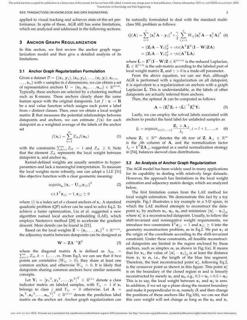
be naturally formulated to deal with the standard multi-class SSL problem as follows:

Q(A) =l∑

i=1

∥zTi A− yi∥2+γ

2

n∑i,j=1

Wij∥zTi A− zTj A∥2 (4)

= ∥ZlA−Yl∥2F + γtr(ATZT(I−W)ZA)

= ∥ZlA−Yl∥2F + γtr(ATLA)

where L = ZT(I−W)Z ∈ Rm×m is the reduced Laplacian,Zl ∈ Rl×m is the sub-matrix according to the labeled part oflocal weight matrix Z, and γ > 0 is a trade-off parameter.

From the above equation, we can see that, althoughAGR is performed with a regularization on all datapoint,it is equivalent to a regularization on anchors with a graphLaplacian L. This is understandable, as the labels of otherdatapoints are actually inferred from anchors.

Then, the optimal A can be computed as follows

A = (ZTl Zl + γL)

−1ZT

l Yl (5)

Lastly, we can employ the solved labels associated withanchors to predict the hard label for unlabeled samples as

yi = argmaxj∈{1,...,c}Zi· ×A·j

λj, i = l + 1, . . . , n (6)

where Zi· ∈ Rm denotes the ith row of Z, A·j ∈ Rm

is the jth column of A, and the normalization factorλj = 1TZA·j , suggested as a useful normalization strategyin [54], balances skewed class distributions.

3.2 An Analysis of Anchor Graph RegularizationThe AGR model has been widely used in many applicationsfor its capability in dealing with relatively large datasets.However, the approach has limitations in the local weightestimation and adjacency matrix design, which are analyzedbelow.

The first limitation comes from the LAE method forlocal weight estimation. We demonstrate this fact by a toyexample. Fig.1 illustrates a toy example in a 3-D space, inwhich the LAE method attempts to reconstruct the data-point x1 by anchors u1, u2, u3 and minimizes ∥x′

1 − x1∥2,where x′

1 is a reconstructed datapoint. Usually, to follow theshift-invariant and nonnegative weight requirements, weintroduce two constraints 1Tz⟨i⟩ = 1 and z⟨i⟩ ≽ 0 into thegeometry reconstruction problem, as in Eq.2. We put x1 atthe origin of the coordinate according to the shift-invariantconstraint. Under these constraints, all feasible reconstruct-ed datapoints are limited in the region enclosed by theseanchors, such as simplex α, as shown in Fig.1(a). It meansthat for x1, the value of ∥x′

1 − x1∥2 is at least the distancefrom x1 to α, i.e., the length of the blue line segment.Therefore, the best reconstructed point x∗

1, following Eq.2,is the crossover point as shown in this figure. This point x∗

1

is on the boundary of the closed region α and is linearlyreconstructed by merely u1 and u2, e.g., 0.5×u1+0.5×u2.This is to say, the local weight between x1 and u3 is zero.In addition, if we set up a plane along the nearest boundaryand make it perpendicular to α, namely β, and then changethe positions of these anchors like Fig.1(b), we can see thatthis zero weight will not change as long as the u3 and x1




Fig. 1. A 3-D toy example for datapoint reconstruction with anchors.

(a) a part of local weight matrix

(b) local edges for these points

Fig. 2. An example to model the adjacency.

are at different sides of the plane β, even if u3 is closer tox1 than u1 and u2, because the best reconstructed point x∗

1

is still on the boundary. As shown in Fig.1(c), only when u3

and x1 are at the same side of β, the x∗1 will move inside

the simplex α, and the previous zero weight can changeto a positive value. We have discussed the situation abovewhere s = 3. However, this geometric interpretation canalso be easily extended to the case where s > 3. FromFig.1(d), we can see the difference is that the region enclosedby anchors now becomes a closed space, i.e., α′, and β′ nowlies along the boundary simplex of α′ which is closest to x1.Similarly, from this figure, we can see that the local weightbetween x1 and the anchor, which is on the opposite spaceof β′, namely u4, is always zero. In addition to the aboveproblem, computational cost can also be a disadvantage ofLAE, despite several strategies have been applied in [21] tospeed up the process.

The second limitation is the adjacency matrix design.After describing the local connection between datapointsand their neighboring anchors, we consider building theadjacency relationship in the whole data space for graphregularization. For instance, we obtain a part of localweights as listed in Fig.2(a). To view these values graph-ically, we also use a toy example in Fig.2(b) to show therelationship between these points, where the length of the

edge represents the Euclidean distance between the dat-apoints and anchors. Now, if we calculate the adjacencyweight according to Eq.3 with these local weights, we haveW12 =

∑mk=1

Z1kZ2k

Λkk= 0.3×0.4

Λ11+ 0.4×0.3

Λ22+ 0.3×0.3

Λ33and

W34 =∑m

k=1Z3kZ4k

Λkk= 0.1×0.1

Λ11+ 0.1×0.1

Λ22+ 0.8×0.8

Λ33. Further,

if we suppose that Λkk is nearly the same in homogeneousregions, such as in Fig.2(b), we can obtain W12 = 0.33

Λkkand

W34 = 0.66Λkk

. In this context, the adjacency weights of x1&x2

and x3&x4 can be numerically quite different, althoughthe Euclidean distances between them are nearly the same.Therefore, this issue is likely to introduce mistakes in theremaining steps of graph-based SSL tasks.

4 EFFICIENT ANCHOR GRAPH REGULARIZATION

To address the above issues in AGR, we accordingly pro-pose two improvements. First, we introduce a fast localanchor embedding method in anchor graph construction,which reformulates the local weight estimation problem tobetter measure Z and speeds up optimization. Second, wedirectly design a normalized graph Laplacian over anchorsand show that it is more effective than the reduced graphLaplacian in AGR. More details are given in the following.




4.1 Fast Local Anchor EmbeddingApart from LAE described above, there exist other similarmethods for local weight estimation like LLE [31], LLC[39], and LLA [41]. However, these methods either do notenforce weights to be non-negative or impose the non-negative constraint into objective function via inequality. Inthe former cases, non-negative similarity measures cannotbe guaranteed. In the latter cases, limitation still exists whendatapoints are outside of the convex envelope of anchors,according to the analysis in Section 3.2. Therefore, here weaim to design a better local weight matrix Z to tackle theseproblems. We call our new weight estimation method FastLocal Anchor Embedding (FLAE) as we will demonstratethat the optimization problem has an analytical solution andcan be implemented fast. It is worth mentioning here that,although we use a close name, the formulation of FLAE andits solution are actually quite different from the conventionalLAE method. In fact, we have made two changes.

Change 1. Instead of the inequality constraint, we useabsolute constraint in geometric reconstruction. Since thenon-negative property in similar measurement is impor-tant to guarantee the global optimum of graph-based SSL[21], inequality constraint has been employed in most localweight estimation methods, e.g. LAE and LLA. However,as illustrated in Section 3.2, it would introduce additionalmistakes when the datapoint is outside of convex envelopeof anchors. Therefore, we integrate the non-negative prop-erty from another perspective: absolute operator. To thisend, we set z⟨i⟩ = |c⟨i⟩| and the constraint 1T|c⟨i⟩| = 1is imposed to follow the shift-invariant requirement in ourgeometric reconstruction problem. Then, we can obtain thelocal weight vector z⟨i⟩ for each datapoints xi, correspond-ing to the following problem:

argminci∥xi −U⟨i⟩c⟨i⟩∥

2 (7)

s.t.1T|c⟨i⟩| = 1

Compared with LAE, Eq.7 can be a more direct modelto handle the non-negative property in similarity measure.However, since there lacks a straightforward solution ofthe optimization problem, here we obtain a solution viashrinking the domain of the above problem.

Specifically, we first drop the absolute constraint in ourmodel, which reduces the problem to a simple coding prob-lem as:

argminc⟨i⟩∥xi −U⟨i⟩c⟨i⟩∥

2 (8)

s.t.1Tc⟨i⟩ = 1

And the solution can be derived analytically by:

c⟨i⟩ = Ci−11 (9)

c⟨i⟩ = c⟨i⟩/1Tc⟨i⟩ (10)

where Ci = (UT⟨i⟩ − 1xi

T)(UT⟨i⟩ − 1xi

T)T ∈ Rs×s is a data

covariance matrix.Then, we compute our local weight vector z⟨i⟩ after

obtaining the code c⟨i⟩ as follows:

ρ = 1T|c⟨i⟩| (11)

c⟨i⟩ = c⟨i⟩/ρ (12)

z⟨i⟩ = |c⟨i⟩| (13)

As we can see, the above solution c⟨i⟩ satisfies the con-straint 1T|c⟨i⟩| = 1, it means this c⟨i⟩ is a feasible solutionof Eq.7. Meanwhile, we can have the following conclusion.

PROPOSITION 1. The minimum of Eq.8 will not notgreater than the minimum of Eq.2.

We leave the proof of the proposition to appendix.Then, our task is to demonstrate that, with the above

solution, the value of the objective function in Eq.7 is notgreater than the value of Eq.8 with its optimal solution c⟨i⟩.If this conclusion can be drawn, it means that our methodcan lead to a smaller reconstruction error than LAE, and theeffectiveness of our approach can be validated. The detailsare as follows.

Recall that, by solving Eq.8, we obtain the optimal solu-tion c⟨i⟩. Clearly, there are two possible cases regarding theobtained codes cij ∈ c⟨i⟩ : (1) ∀ cij ≥ 0; and (2) ∃ cij < 0.Then, we follow Eqs.11-12 to yield codes c⟨i⟩.

For the first case, we obtain c⟨i⟩ = c⟨i⟩. It means thatthe value of the objective function in Eq.7 with our feasiblesolution is the same with the value of Eq.8 with its optimalsolution.

We then mainly focus on the second case. Since theobtained code c⟨i⟩ satisfies the constraint 1Tc⟨i⟩ = 1, wefirst substitute it into the objective function in Eq.8 to yieldthe minimum of Eq.8 as

∥x⟨i⟩1Tc⟨i⟩ −U⟨i⟩c⟨i⟩∥

2= ∥U⟨i⟩c⟨i⟩∥

2(14)

where U⟨i⟩ = [U⟨i⟩(:, 1) − xi, . . . ,U⟨i⟩(:, s) − xi] can beviewed as the new coordinates of the s closest anchors of xi

in the datapoint-centered coordinate system.Then, according to Eqs.11-12, we scale the code c⟨i⟩ in

Eq.14 by a constant ρ and obtain the value of the objectivefunction in Eq.7 with our feasible solution c⟨i⟩:

∥U⟨i⟩c⟨i⟩∥2= ∥1

ρU⟨i⟩c⟨i⟩∥

2

=1

ρ2∥U⟨i⟩c⟨i⟩∥

2(15)

Since ∃ cij < 0, we have ρ > 1. Therefore, we obtainthe inequality relation that the value of Eq.15 is smaller thanEq.14.

Up to now, we have demonstrated that the value of theobjective function in Eq.7 with our feasible solution is notgreater than the value of Eq.8 with its optimal solution,which means we can obtain a smaller reconstruction errorthan LAE. Moreover, our analytical solution based on Eqs.9-13 is much faster than the iterative solution obtained byLAE.

Change 2. We further incorporate the locality constraintsinto local weight estimation. To enhance coding efficiency,the locality constraint functions in other similar methods[21], [41] are replaced by using the s closest anchors (land-marks), like approximated LLC [39] does. However, thismanipulation is insufficiently suitable, because it ignores thereal distance between local points (an negative example isshown in Fig.1(b)). We therefore suggest keeping the localityconstraint while using the s closest anchors in local weightestimation simultaneously.




We obtain local weight vector z⟨i⟩ = |c⟨i⟩| according tothe following objective:

argminci∥xi −U⟨i⟩c⟨i⟩∥

2+ λ∥d⟨i⟩ ⊙ c⟨i⟩∥

2 (16)

s.t.1T|c⟨i⟩| = 1

where ⊙ denotes the element-wise multiplication. d⟨i⟩ isthe locality adaptor that allows a different freedom foreach anchor proportional to its distance to the datapoint xi.Specifically,

d⟨i⟩ = exp(∥xi −U⟨i⟩∥2

σ) (17)

where the parameter σ is used to adjust the weight decayspeed for the locality adaptor.

Similarly, we can obtain a feasible solution as before. Theonly change compared to the pervious processes is that wereplace Eq.9 with

c⟨i⟩ = (Ci + λdiag(d⟨i⟩))−1

1 (18)

To summarize, we demonstrate the steps of FLAE inAlgorithm 1.

Algorithm.1 Fast Local Anchor Embedding (FLAE).Input: datapoints {xi}ni=1 ∈ Rd, anchor set obtainedfrom K-means U ∈ Rm×d, parameters s and λ.for i = 1 to n do

1. For xi, find s nearest neighbors in U and recordthe index set ⟨i⟩.

2. Measure the locality adaptor d⟨i⟩ for datapointxi with its nearest neighbors U⟨i⟩ via Eq.17.

3. Compute the code c⟨i⟩ via Eq.18, and Eqs.10-12.4. Obtain the final solution z⟨i⟩ via Eq.13.5. Zi,⟨i⟩ = zT⟨i⟩.

end forOutput: FLAE matrix Z .

4.2 Normalized Graph Laplacian over Anchors

Fig. 3. A toy example of the nearest anchors of datapoints.

We consider a graph as a stable one if it satisfies thecluster assumption, which means nearby datapoints arelikely to have the same labels. Obviously, it is important forbuilding a well performed anchor-graph-based SSL classifi-cation model. In Section 3.2, we have observed the limitationof the anchor graph built based on the conventional adjacen-cy between datapoints. As demonstrated in Section 3.1, inanchor graph regularization, the regularization on all dat-apoints is actually equivalent to regularization on anchorswith a reduced graph Laplacian, which is built over onlyanchors. Therefore, here we directly design an adjacencymatrix among anchors and then derive a normalized graphLaplacian over anchors. For clarity, we use the subscripts

i, j, k and s, t, r to denote the indices of datapoints andanchors respectively in this subsection. The details are asfollows.

Recall that the label for each datapoint is estimated asa weighted average of the labels of the anchor set via Eq.1,which only involves the local weight vector of the datapointand the labels of its nearest anchors. Given local weights, thelabel vectors of the nearest anchors are crucial to the finallabel prediction for the datapoint. If two nearby datapointsshare a lot of nearest anchors, their labels are likely to besimilar. However, nearby datapoints are not guaranteed tohave identical nearest anchors quite often. Fig.3 illustrates atoy example, where the nearest anchors of nearby pairwisedatapoints x1 and x2 are the same while those of x1 and x3

are not. We prefer the Laplacian matrix has the followingcharacteristics: 1) the elements corresponding to the nearbypairwise anchors should be negative, which means theseanchors tend to have similar labels; 2) the elements cor-responding to dissimilar pairwise anchors should be zero,which means their labels are irrelevant [27]. To this end, wedesign the adjacency matrix between anchors as:

W = ZTZ (19)

where Wst =∑n

k=1 ZksZkt. Accordingly, its normalizedLaplacian matrix is :

L = I−D−1/2WD−1/2 (20)

where the diagonal matrix D is defined as Dss =∑m

t=1 Wst.Note that our adjacency matrix actually explores all data-points as the transitional points rather than anchors alone.Thus, our model keeps the computational efficiency of theanchor graph regularization and its effectiveness in regular-ization.

As for AGR, it constructs an n × n adjacency matrix asW = ZΛ−1ZT. Based on this, AGR employs the followingreduced Laplacian matrix L over anchors for its regulariza-tion function:

L = ZT(I− ZΛ−1ZT)Z (21)

= ZTZ− ZT(ZΛ−1ZT)Z

Now we compare the two m×m Laplacian matrices overanchors, according to the previously mentioned characteris-tics. For convenience, we take a non-diagonal element Lst

for example, which is computed as

Lst =

{−αZT

·sZ·t for EAGRZT

·sZ·t − ZT·s(ZΛ

−1ZT)Z·t for AGR(22)

where α = (DssDtt)− 1

2 , Z·s ∈ Rn denotes the sth col of Z.We discuss the sign of Lst in the following two cases

according to the relations of the pairwise anchors us&ut.1) The first case is that us&ut share at least one common

datapoint xi, namely, they are nearby. For EAGR, we clearlyhave Lst = −αZT

·sZ·t ≤ −αZisZit < 0. However, forAGR, the sign of the element Lst depends on the valuesof ZT

·sZ·t and ZT·s(ZΛ

−1ZT)Z·t. Therefore, the element Lst

can be positive, zero, or negative. If Lst > 0, these nearbyanchors tend to have different labels. If Lst = 0, thesenearby anchors tend to be irrelevant. When Lst < 0, wecan obtain the expected result, that is, nearby anchors tend




to have similar labels. In short, the labels of nearby pairwiseanchors in EAGR are enforced to be similar, while this isuncertain for AGR.

2) The second case is that us&ut does not share anycommon datapoint, namely, they are dissimilar. For EAGR,we have Lst = −αZT

·sZ·t = 0. However, for AGR, althoughZT

·sZ·t is zero, ZT·s(ZΛ

−1ZT)Z·t may still be positive, whichmakes Lst negative. For example, anchors us&ut connectwith two different datapoints xi&xj respectively, and thesedatapoints share another anchor ur simultaneously. Then,we obtain Lst < 0, since Lst = 0 − ZT

·s(ZΛ−1ZT)Z·t <

0−Zis(ZΛ−1ZT)ijZjt, where (ZΛ−1ZT)ij ≥ ZirΛ

−1rr Zjr >

0 and Zis > 0, Zjt > 0. Therefore, unexpected negativeLaplacian weights could exist between dissimilar anchorsin AGR model while our EAGR is free from this situation.

Later in Section 5.2, based on real-world datasets, wewill show several examples by comparing the number ofnonzero elements at the non-diagonal positions of the abovem × m Laplacian matrices. In conclusion, based on theproposed W, we can better describe the adjacency betweenanchors and make the smoothness constraint more effectivefor the stable anchor graph construction. As the commonlinked datapoints are used as transitional points in buildingW, we note that our adjacency matrix W is totally differentfrom the simple kNN graph, which only depends on thesparse anchors themselves.

4.3 Learning on Anchor GraphNow we consider a standard multi-class SSL task. Givena set of labeled datapoints xi (i = 1, . . . , l) with the corre-sponding discrete label yi ∈ {1, . . . , c}, our goal is to predictthe labels on the remaining unlabeled real datapoints asso-ciated with anchors. Let Yl = [y1

T,y2T, . . . ,yl

T]T ∈ Rl×c

denote a class indicator matrix on labeled datapoints withYij = 1 if xi belongs to class j and Yij = 0 otherwise.Suppose that, for each datapoint, we obtain a label predic-tion function f i = zTi A where A = [a1

T,a2T, . . . ,am

T]T ∈

Rm×c denotes the prediction label matrix on the anchor set.Specifically, ai ∈ R1×c is the label vector of the anchor ui.Then, we combine anchors with datapoints to build a modelcalled Efficient Anchor-Graph Regularization (EAGR) forSSL as follows

argminA

l∑i=1

∥zTi A− yi∥2+

γ

2

m∑i,j=1

Wij∥ai√Dii

− aj√Djj

∥2

(23)We can also present this optimization problem in the

following matrix form

argminA∥ZlA−Yl∥2F + γtr(ATLA) (24)

where L = I−D−1/2WD−1/2 ∈ Rm×m is the previouslyintroduced normalized Laplacian matrix, ∥·∥F stands for theFrobenius norm, and γ > 0 is the trade-off parameter.

With simple algebra, we can obtain a globally optimalsolution for the anchors’ label matrix as follows

A = (ZTl Zl + γL)

−1ZT

l Yl (25)

This yields a closed-form solution for handling largescale SSL tasks. Lastly, like AGR, we utilize the local weight

matrix with anchors’ soft scores to predict the hard labelsfor unlabeled datapoints as Eq.6.

To summarize, our EAGR consists of the following steps:(1) finding anchors by K-means; (2) estimating the localweight matrix Z by FLAE, as illustrated in Algorithm 1;(3) computing the normalized Laplacian matrix L overanchors via Eq.20; (4) carrying out the graph regularizationvia Eq.25; and (5) predicting the hard labels on unlabeleddatapoints via Eq.6. As we can see, our EAGR keeps thesimplicity of AGR and tends to be much faster, since itefficiently solves the local weight estimation with FLAE. Tobe clear, Table 1 and Table 2 show the storage costs and timecomplexity of several semi-supervised learning algorithms,where n is the number of datapoints, m is the number of an-chors, s is the number of the closest anchors to a datapoint, dis the dimension of features, and t is the number of iterationsin the corresponding iterative optimization process.

5 EXPERIMENTS

5.1 Data Settings

To evaluate the performance of our EAGR, we conduct ex-periments on five widely-used handwritten datasets: BinaryAlphadigits1 (Alphadigits for short), USPS1, MNIST1, Se-meion2, and Letter Recognition2 (Letter for short). Followingthe settings of [21], we divide them into three groups basedon their sizes, that is, number of samples. It is worthwhile tonote that the images in Letter have already been convertedinto 16 primitive numerical attributes (statistical momentsand edge counts) to represent each sample. In other datasets,samples are still pixel images of different size. For thesedatasets, we directly use a high-dimensional vector of nor-malized grayscale values to represent each instance. Theattributes of these datasets are listed in Table 3. All theexperiments are implemented on a 2.4 GHz CPU, 32GBRAM PC.

5.2 On the two improvements in EAGR

Before comparing our EAGR with other methods, we con-duct two experiments to validate the effectiveness of the twoimprovements described in Section 4.1 and 4.2 respectively.For a fair comparison, we define two intermediate versionsbetween AGR and EAGR as:

(1). AGR+, which employs FLAE for estimating Z anduse the reduced Laplacian matrix in Eq.21.

(2). EAGR- , which employs LAE for estimating Z anduse the normalized Laplacian matrix in Eq.20.

The differences of the methods for comparison are alsosummarized in Table 4. For the involved parameters, wesimply set anchor number to 500 and empirically set s to 3to make the anchor graph sparse. We tune other parameters,i.e., λ and γ, to their optimal values. In this way, we can pro-vide a fair comparison for these algorithms. We randomlyselect 10 labeled samples per class and leave the remainingones unlabeled for SSL models in this subsection.

Table 5 shows the classification accuracies of the fourdifferent methods. Table 6 presents the average CPU time

1available at http://cs.nyu.edu/ roweis/data.html2available at http://archive.ics.uci.edu/ml/




TABLE 1Comparison of storage costs of three graph-based methods.

Approach StorageLearning with local and global consistency (LLGC) [51] O(n2)Anchor Graph Regularization (AGR) [21] O(mn)Efficient Anchor Graph Regularization (EAGR) O(mn)

TABLE 2Comparison of computational complexities of three graph-based methods.

Approach Find anchors Design Z (reduced) graph LaplacianL Graph RegularizationLLGC O(dn2) O(n3)AGR O(mndt) O(mns+ s2dnt) O(m2n) O(m2n+m3)EAGR O(mndt) O(mns+ s2dn) O(m2n) O(m2n+m3)

TABLE 3Details of the five datasets.

Alphadigits Semeion USPS Letter MNIST# of instances 1,404 1,593 11,000 20,000 60,000# of categories 36 10 10 26 10# of features 320 256 256 16 784

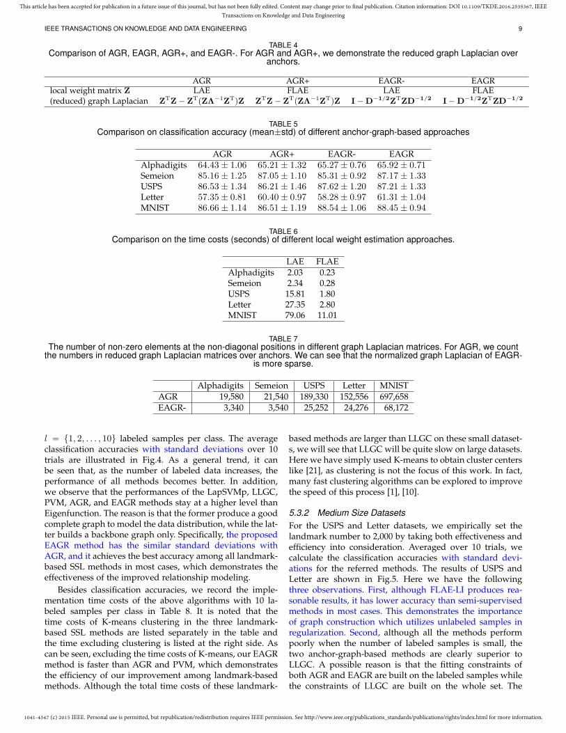
(in seconds) of two local estimation methods on differen-t datasets. Meanwhile, Table 7 illustrates the number ofnonzero elements at the non-diagonal positions in differentLaplacian matrices as mentioned in Sectioin 4.2. From theresults, we have two observations as follows.

First, by comparing AGR+ with AGR, we see that theformer has comparable or better performances than thelatter. In addition, Table 6 reveals that our proposed FLAE inAGR+ is much faster than LAE in AGR. These performancesdemonstrate the efficiency of our improvement on the localweight estimation.

Second, by comparing EAGR- with AGR, we see that, al-though two methods use the same optimized Z, the EAGR-has better classification performance than AGR on all fivedatasets. We can see from Table 7 that the normalized graphLaplacian of EAGR- has less non-zero elements than thereduced graph Laplacian of AGR. This means that, with asparse normalized graph Laplacian, several incorrect linkshave been removed.

5.3 Comparison with other methods

Here we further compare the proposed EAGR approachwith the following methods.

(1) FLAE-based label inference, which constructs thelocal matrix between unlabeled datapoints and the labeledones with FLAE, and then predicts labels for unlabeleddatapoints. This method actually introduces FLAE into thekernel regression approach [3], since each row vector zi ofZ is non-negative and normalized. The method is denotedas “FLAE-LI”.

(2) The Eigenfunctions method introduced in [11], whichsolves the semi-supervised problem in a dimension-reducedfeature space by only working with a small number ofeigenvectors of the Laplacian. The method is denoted as“Eigenfucntion”.

(3) Laplacian Support Vector Machines Trained in thePrimal with preconditioned conjugate gradient, which isintroduced in [26]. We first decompose a c-class classifi-cation problem into c one-versus-rest binary classificationproblems. Prediction is then made by assigning the sampleto the class with the highest decision function value. Themethod is denoted as “LapSVMp”.

(4) Learning with local and global consistency in [51],which is a typical graph-based learning method. It directlycomputes the affinity matrix with Gaussian kernel. In ourexperiments, we use the 6NN strategy in graph construc-tion and use Gaussian kernel for weighting the edges. Themethod is denoted as “LLGC”.

(5) Prototype Vector Machines with the Square Loss in[47], [48], which is a scale-up graph-based semi-supervisedlearning for multi-label classification tasks using a set ofsparse prototypes derived from the data and the Gaussiankernel is used to define the graph affinity. The method isdenoted as “PVM”.

(6) Anchor Graph Regularization, which employs clus-tering centers as anchors with LAE, is proposed in [21]. Itis the prime counterpart in our experiments, and we aim toimprove its performance. The method is denoted as “AGR”.

Since the last two methods and EAGR are based oneither the anchors or the prototypes, we group them into“landmark-based learning” methods and perform K-meansto obtain these cluster centers as the landmarks. Aiming ata fair comparison, the radius parameters of the Gaussiankernel in the methods (2-4) are set by 5-fold cross-validation.The trade-off parameters in regularization of the abovemethods are empirically tuned to their optimal values.

5.3.1 Small Size DatasetsWe first conduct experiments on two small datasets: Al-phadigits and Semeion. For the three landmark-based meth-ods, we empirically set the landmark number to 500 and




TABLE 4Comparison of AGR, EAGR, AGR+, and EAGR-. For AGR and AGR+, we demonstrate the reduced graph Laplacian over

anchors.

AGR AGR+ EAGR- EAGRlocal weight matrix Z LAE FLAE LAE FLAE(reduced) graph Laplacian ZTZ− ZT(ZΛ−1ZT)Z ZTZ− ZT(ZΛ−1ZT)Z I−D−1/2ZTZD−1/2 I−D−1/2ZTZD−1/2

TABLE 5Comparison on classification accuracy (mean±std) of different anchor-graph-based approaches

AGR AGR+ EAGR- EAGRAlphadigits 64.43± 1.06 65.21± 1.32 65.27± 0.76 65.92± 0.71Semeion 85.16± 1.25 87.05± 1.10 85.31± 0.92 87.17± 1.33USPS 86.53± 1.34 86.21± 1.46 87.62± 1.20 87.21± 1.33Letter 57.35± 0.81 60.40± 0.97 58.28± 0.97 61.31± 1.04MNIST 86.66± 1.14 86.51± 1.19 88.54± 1.06 88.45± 0.94

TABLE 6Comparison on the time costs (seconds) of different local weight estimation approaches.

LAE FLAEAlphadigits 2.03 0.23Semeion 2.34 0.28USPS 15.81 1.80Letter 27.35 2.80MNIST 79.06 11.01

TABLE 7The number of non-zero elements at the non-diagonal positions in different graph Laplacian matrices. For AGR, we count

the numbers in reduced graph Laplacian matrices over anchors. We can see that the normalized graph Laplacian of EAGR-is more sparse.

Alphadigits Semeion USPS Letter MNISTAGR 19,580 21,540 189,330 152,556 697,658EAGR- 3,340 3,540 25,252 24,276 68,172

l = {1, 2, . . . , 10} labeled samples per class. The averageclassification accuracies with standard deviations over 10trials are illustrated in Fig.4. As a general trend, it canbe seen that, as the number of labeled data increases, theperformance of all methods becomes better. In addition,we observe that the performances of the LapSVMp, LLGC,PVM, AGR, and EAGR methods stay at a higher level thanEigenfunction. The reason is that the former produce a goodcomplete graph to model the data distribution, while the lat-ter builds a backbone graph only. Specifically, the proposedEAGR method has the similar standard deviations withAGR, and it achieves the best accuracy among all landmark-based SSL methods in most cases, which demonstrates theeffectiveness of the improved relationship modeling.

Besides classification accuracies, we record the imple-mentation time costs of the above algorithms with 10 la-beled samples per class in Table 8. It is noted that thetime costs of K-means clustering in the three landmark-based SSL methods are listed separately in the table andthe time excluding clustering is listed at the right side. Ascan be seen, excluding the time costs of K-means, our EAGRmethod is faster than AGR and PVM, which demonstratesthe efficiency of our improvement among landmark-basedmethods. Although the total time costs of these landmark-

based methods are larger than LLGC on these small dataset-s, we will see that LLGC will be quite slow on large datasets.Here we have simply used K-means to obtain cluster centerslike [21], as clustering is not the focus of this work. In fact,many fast clustering algorithms can be explored to improvethe speed of this process [1], [10].

5.3.2 Medium Size DatasetsFor the USPS and Letter datasets, we empirically set thelandmark number to 2,000 by taking both effectiveness andefficiency into consideration. Averaged over 10 trials, wecalculate the classification accuracies with standard devi-ations for the referred methods. The results of USPS andLetter are shown in Fig.5. Here we have the followingthree observations. First, although FLAE-LI produces rea-sonable results, it has lower accuracy than semi-supervisedmethods in most cases. This demonstrates the importanceof graph construction which utilizes unlabeled samples inregularization. Second, although all the methods performpoorly when the number of labeled samples is small, thetwo anchor-graph-based methods are clearly superior toLLGC. A possible reason is that the fitting constraints ofboth AGR and EAGR are built on the labeled samples whilethe constraints of LLGC are built on the whole set. The




1 2 3 4 5 6 7 8 9 100.25

0.3

0.35

0.4

0.45

0.5

0.55

0.6

0.65

0.7

number of labeled samples per class

clas

sific

atio

n ac

cura

cy

FLAE−LIEigenfunctionLapSVMpLLGCPVMAGREAGR

(a) Alphadigits

1 2 3 4 5 6 7 8 9 100.2

0.3

0.4

0.5

0.6

0.7

0.8

0.9


clas

sific

atio

n ac

cura

cy


(b) Semeion

Fig. 4. Classification accuracy vs. the number of labeled samples on small-size datasets.

TABLE 8Time costs (seconds) of the compared learning algorithms on small-size datasets.

Landmark-based Learning OthersK-means AGR EAGR PVM FLAE-LI Eigenfunction LapSVMp LLGC

Alphadigits 2.10 +2.17 +0.28 +0.32 0.14 0.95 7.25 0.73Semeion 2.01 +2.48 +0.30 +0.34 0.13 0.73 1.13 0.83

1 2 3 4 5 6 7 8 9 100.2

0.3

0.4

0.5

0.6

0.7

0.8

0.9


clas

sific

atio

n ac

cura

cy


(a) USPS

1 2 3 4 5 6 7 8 9 100.2

0.25

0.3

0.35

0.4

0.45

0.5

0.55

0.6

0.65

0.7


clas

sific

atio

n ac

cura

cy


(b) Letter

Fig. 5. Classification accuracy vs. the number of labeled samples on medium-size datasets.

TABLE 9Time costs (seconds) of the compared learning algorithms on medium-size datasets.


USPS 59.00 +20.72 +4.45 +16.43 0.69 4.95 56.68 120.67Letter 11.15 +35.42 +7.16 +25.04 1.14 1.09 139.39 432.73




fitting effects of AGR and EAGR, therefore, are more biasedtowards labeled information than that of LLGC. Third, whenthe number of labeled samples increases, the performancesof all methods become better and the accuracy of EAGRimproves more significantly than AGR. The reason is that,as the number of labeled samples increases, these classi-fiers model the characteristics of different classes better.However, this increase also makes the classifiers tend tobe overfitted, which needs to be handled by an effectivesmoothness constraint. Owning to the better relationshipmodeling in the data space to meet this requirement, EAGRaddresses the limitation of AGR as expected.

We also demonstrate the implementation time costs ofthe above algorithms with 10 labeled samples per class inTable 9. We can observe that, although LapSVMp is fasterthan LLGC, it is still computationally expensive on thelarger data set, e.g., Letter, as its time complexity is quadraticwith respect to n. The landmark-based learning algorithms,especially EAGR, need much less implementation costs thanLLGC. In addition, the K-means clustering process accountsfor the main portion of the EAGR’s time cost. Therefore, ifwe can reduce the clustering time by employing other fastclustering algorithms [1], [10] or just selecting a part of thedatabase samples to run K-means like [43], the advantage ofour EAGR over the other two in terms of speed is expectedto be greater.

5.3.3 Large Size DatasetFor the MNIST dataset, we empirically set the landmarknumber to 2,000 in the three landmark-based methods. Fig.6shows the results of the algorithms on MNIST. We can ob-serve that the two anchor-graph-based methods are clearlysuperior to LLGC when the number of labeled samples issmall. Similar to the results in the previous experiments,we see that our method achieves better performance thanAGR and PVM. Meanwhile, Table 10 also demonstrates thatour EAGR is more advantageous than the AGR and PVMmethods in terms of speed for the large dataset.

1 2 3 4 5 6 7 8 9 100.4

0.45

0.5

0.55

0.6

0.65

0.7

0.75

0.8

0.85

0.9


clas

sific

atio

n ac

cura

cy


(a) MNIST

Fig. 6. Classification accuracy vs. the number of labeled sam-ples on the large-size dataset.

5.4 On the Parameters λ and γ

Finally, we test the sensitivity of the two parameters λ andγ involved in the proposed algorithm. For convenience, wesimply set anchor number to 500 and empirically set s = 3 .We first set γ to 1 and vary λ from 0.001 to 1000. Fig.7 showsthe performance curve with respect to the variation of λ.From the figure, we observe that our method consistentlyoutperforms AGR, and the performances stay at a stablelevel over a wide range of parameter variation. We thenvary the value of γ from 0.001 to 1000 for both EAGRand AGR (λ = 10). Fig.8 demonstrates the performancevariation. We can see that EAGR is superior to AGR whenγ varies in a wide range and the curve of EAGR has a peakwhen γ = 1 in most cases. These observations demonstratethe robustness of the parameter selection in applying ourmethod to different datasets.

6 CONCLUSION

This work introduces a novel scalable graph-based semi-supervised learning algorithm named Efficient AnchorGraph Regularization (EAGR). It improves the AGR ap-proach in the following two aspects. First, in anchor graphconstruction, it employs a novel fast local anchor embed-ding method to better measure the local weights betweendatapoints and neighboring anchors. Second, in anchorgraph regularization, it employs a novel normalized graphLaplacian over anchors, which works better than the re-duced graph Laplacian in AGR. For each improvement,we have provided an in-depth analysis on the limitationof the conventional method and the advantages of the newmethod. Experiments on publicly available datasets of vari-ous sizes have validated our EAGR in terms of classificationaccuracy and computational speed.

APPENDIXPROOF OF PROPOSITION 1First, we present the following lemma.

LEMMA 1. Suppose f1 is the minimization problem withobjective function g in domain A, f2 is the minimizationproblem with the same objective function g in domain B,and B ⊂ A, then for the optimal solution to f1, e.g., xA, andthe optimal solution to f2, e.g., xB , we have g(xA) ≤ g(xB).

The proof of the above lemma is clear. Since xB is theoptimal solution to f2 in domain B, we have xB ∈ B. NoteB ⊂ A, so xB ∈ A. Therefore, if g(xA) > g(xB), xA is notthe optimal solution to f1 in domain A.

Now we prove Proposition 1. Clearly, both Eq.8 and Eq.2have the same objective function. In addition, if A denotesthe domain of Eq.8, i.e., 1Tc⟨i⟩ = 1 and B denotes thedomain of Eq.2, i.e.,1Tz⟨i⟩ = 1, z⟨i⟩ ≽ 0, we have B ⊂ A.According to LEMMA 1, the minimum of Eq.8 is not greaterthan the minimum of Eq.2, which completes the proof.

REFERENCES

[1] J. S. Beis and D. G. Lowe, “Shape indexing using approximatenearest-neighbour search in high-dimensional spaces,” in Pro-ceedings of the IEEE Conference on Computer Vision and PatternRecognition (CVPR), 1997, pp. 1000–1006.




10−2

100

102

0.63

0.635

0.64

0.645

0.65

0.655

0.66

0.665

0.67

values of λ

aver

age

clas

sific

atio

n ac

cura

cy

AGR

500

EAGR500

(a) Alphadigits

10−2

100

102

0.85

0.86

0.87

0.88

values of λ

aver

age

clas

sific

atio

n ac

cura

cy

AGR

500

EAGR500

(b) Semeion

10−2

100

102

0.84

0.85

0.86

0.87

0.88

0.89

values of λ

aver

age

clas

sific

atio

n ac

cura

cy

AGR

500

EAGR500

(c) USPS

10−2

100

102

0.54

0.56

0.58

0.6

0.62

0.64

values of λ

aver

age

clas

sific

atrio

n ac

crac

y

AGR

500

EAGR500

(d) Letter

10−2

100

102

0.86

0.87

0.88

0.89

values of λ

aver

age

clas

sific

atio

n ac

cura

cy

AGR

500

EAGR500

(e) MNIST

Fig. 7. Average performance curves of EAGR with respect to the variation of λ. Here, the number of labeled samples is set to10 per class.

10−2

100

102

0.4

0.45

0.5

0.55

0.6

0.65

0.7

values of γ

aver

age

clas

sific

atio

n ac

cura

cy

AGR500

EAGR500

(a) Alphadigits

10−2

100

102

0.78

0.8

0.82

0.84

0.86

0.88

values of γ

aver

age

clas

sific

atio

n ac

cura

cy

AGR500

EAGR500

(b) Semeion

10−2

100

102

0.84

0.85

0.86

0.87

0.88

values of γ

aver

age

clas

sific

atio

n ac

cura

cy

AGR

500

EAGR500

(c) USPS

10−2

100

102

0.5

0.52

0.54

0.56

0.58

0.6

0.62

values of γ

aver

age

clas

sific

atio

n ac

cura

cy

AGR

500

EAGR500

(d) Letter

10−2

100

102

0.86

0.87

0.88

0.89

values of γ

aver

age

clas

sific

atio

n ac

cura

cy

AGR

500

EAGR500

(e) MNIST

Fig. 8. Average performance curves of EAGR and AGR with respect to the variation of γ. Here, the number of labeled samplesis set to 10 per class.




TABLE 10Time costs (seconds) of the compared learning algorithms on large-size dataset.


MNIST 168.43 +130.07 +35.15 +87.74 5.59 27.40 3296.71 9521.15

[2] M. Belkin and P. Niyogi, “Semi-supervised learning on riemannianmanifolds,” Machine learning, vol. 56, no. 1-3, pp. 209–239, 2004.

[3] C. M. Bishop, Pattern recognition and machine learning. Springer,2006.

[4] A. Blum and T. Mitchell, “Combining labeled and unlabeled datawith co-training,” in Proceedings of the 11th Annual Conference onComputational Learning Theory (COLT), 1998, pp. 92–100.

[5] D. Cai and X. Chen, “Large scale spectral clustering withlandmark-based representation,” IEEE Transaction on Cybernetics,vol. 45, no. 8, pp. 1669–1680, 2015.

[6] V. Castelli and T. M. Cover, “On the exponential value of labeledsamples,” Pattern Recognition Letters, vol. 16, no. 1, pp. 105–111,1995.

[7] J. Cheng, C. Leng, P. Li, M. Wang, and H. Lu, “Semi-supervisedmulti-graph hashing for scalable similarity search,” Computer Vi-sion and Image Understanding, vol. 124, pp. 12–21, 2014.

[8] C. Deng, R. Ji, W. Liu, D. Tao, and X. Gao, “Visual rerankingthrough weakly supervised multi-graph learning,” in Proceedingsof the IEEE International Conference on Computer Vision (ICCV), 2013,pp. 2600–2607.

[9] C. Deng, R. Ji, D. Tao, X. Gao, and X. Li, “Weakly supervised multi-graph learning for robust image reranking,” IEEE Transactions onMultimedia, vol. 16, no. 3, pp. 785–795, 2014.

[10] C. Elkan, “Using the triangle inequality to accelerate k-means,” inProceedings of the 27th International Conference on Machine Learning(ICML), vol. 3, 2003, pp. 147–153.

[11] R. Fergus, Y. Weiss, and A. Torralba, “Semi-supervised learningin gigantic image collections,” in Proceedings of the Conference onAdvances in Neural Information Processing Systems (NIPS), 2009, pp.522–530.

[12] P. Foggia, G. Percannella, and M. Vento, “Graph matching andlearning in pattern recognition in the last 10 years,” InternationalJournal of Pattern Recognition and Artificial Intelligence, vol. 28,no. 01, pp. 1–40, 2014.

[13] L. Gao, J. Song, F. Nie, Y. Yan, N. Sebe, and H. T. Shen, “Optimalgraph learning with partial tags and multiple features for imageand video annotation,” in Proceedings of the IEEE Conference onComputer Vision and Pattern Recognition (CVPR), 2015, pp. 4371–4379.

[14] M. Guillaumin, J. Verbeek, and C. Schmid, “Multimodal semi-supervised learning for image classification,” in Proceedings of theIEEE Conference on Computer Vision and Pattern Recognition (CVPR),2010, pp. 902–909.

[15] S. Gupta, J. Kim, K. Grauman, and R. Mooney, “Watch, listen &learn: Co-training on captioned images and videos,” in MachineLearning and Knowledge Discovery in Databases, 2008, pp. 457–472.

[16] L. Huang, X. Liu, B. Ma, and B. Lang, “Online semi-supervisedannotation via proxy-based local consistency propagation,” Neu-rocomputing, vol. 149, pp. 1573–1586, 2015.

[17] M. S. T. Jaakkola and M. Szummer, “Partially labeled classificationwith markov random walks,” in Proceedings of the Conference onAdvances in Neural Information Processing Systems (NIPS), vol. 14,2002, pp. 945–952.

[18] T. Joachims, “Transductive inference for text classification usingsupport vector machines,” in Proceedings of the International Confer-ence on Machine Learning (ICML), vol. 99, 1999, pp. 200–209.

[19] S. Kim and S. Choi, “Multi-view anchor graph hashing,” in Pro-ceedings of the IEEE International Conference on Acoustics, Speech andSignal Processing (ICASSP), 2013, pp. 3123–3127.

[20] P. Li, J. Bu, L. Zhang, and C. Chen, “Graph-based local concept co-ordinate factorization,” Knowledge and Information Systems, vol. 43,no. 1, pp. 103–126, 2015.

[21] W. Liu, J. He, and S.-F. Chang, “Large graph construction forscalable semi-supervised learning,” in Proceedings of the 27th Inter-national Conference on Machine Learning (ICML), 2010, pp. 679–686.

[22] W. Liu, J. Wang, and S.-F. Chang, “Robust and scalable graph-

based semisupervised learning,” Proceedings of the IEEE, vol. 100,no. 9, pp. 2624–2638, 2012.

[23] W. Liu, J. Wang, S. Kumar, and S.-F. Chang, “Hashing with graph-s,” in Proceedings of the 28th International Conference on MachineLearning (ICML), 2011, pp. 1–8.

[24] X. Liu and B. Huet, “Concept detector refinement using socialvideos,” in Proceedings of the international workshop on Very-large-scale multimedia corpus, mining and retrieval, 2010, pp. 19–24.

[25] F. D. Malliaros, V. Megalooikonomou, and C. Faloutsos, “Estimat-ing robustness in large social graphs,” Knowledge and InformationSystems, vol. 45, no. 3, pp. 645–678, 2015.

[26] S. Melacci and M. Belkin, “Laplacian support vector machinestrained in the primal,” The Journal of Machine Learning Research,vol. 12, pp. 1149–1184, 2011.

[27] B. Mohar, Y. Alavi, G. Chartrand, and O. Oellermann, “Thelaplacian spectrum of graphs,” Graph theory, combinatorics, andapplications, vol. 2, pp. 871–898, 1991.

[28] Y. Nesterov, Introductory lectures on convex optimization. SpringerScience & Business Media, 2004, vol. 87.

[29] M. Norouzi, A. Punjani, and D. J. Fleet, “Fast exact search inhamming space with multi-index hashing,” IEEE Transactions onPattern Analysis and Machine Intelligence, vol. 36, no. 6, pp. 1107–1119, 2014.

[30] M. Okabe and S. Yamada, “Semisupervised query expansion withminimal feedback,” IEEE Transactions on Knowledge and Data Engi-neering, vol. 19, no. 11, pp. 1585–1589, 2007.

[31] S. T. Roweis and L. K. Saul, “Nonlinear dimensionality reductionby locally linear embedding,” Science, vol. 290, no. 5500, pp. 2323–2326, 2000.

[32] J. Song, Y. Yang, Z. Huang, H. T. Shen, and J. Luo, “Effective multi-ple feature hashing for large-scale near-duplicate video retrieval,”IEEE Transactions on Multimedia, vol. 15, no. 8, pp. 1997–2008, 2013.

[33] Z. Tian and R. Kuang, “Global linear neighborhoods for efficientlabel propagation,” in Proceedings of the SIAM International Confer-ence on Data Mining (SDM), 2012, pp. 863–872.

[34] I. Triguero, S. Garcıa, and F. Herrera, “Self-labeled techniquesfor semi-supervised learning: taxonomy, software and empiricalstudy,” Knowledge and Information Systems, vol. 42, no. 2, pp. 245–284, 2015.

[35] R. R. Vatsavai, S. Shekhar, and T. E. Burk, “A semi-supervisedlearning method for remote sensing data mining,” in Proceedingsof the 17th IEEE International Conference on Tools with ArtificialIntelligence (ICTAI), 2005, pp. 207–211.

[36] D. Wang, F. Nie, and H. Huang, “Large-scale adaptive semi-supervised learning via unified inductive and transductive mod-el,” in Proceedings of the 20th ACM SIGKDD International Conferenceon Knowledge Discovery and Data Mining, 2014, pp. 482–491.

[37] F. Wang and C. Zhang, “Label propagation through linear neigh-borhoods,” IEEE Transactions on Knowledge and Data Engineering,vol. 20, no. 1, pp. 55–67, 2008.

[38] J. Wang, J. Wang, G. Zeng, Z. Tu, R. Gan, and S. Li, “Scalable k-nn graph construction for visual descriptors,” in Proceedings of theIEEE Conference on Computer Vision and Pattern Recognition (CVPR),2012, pp. 1106–1113.

[39] J. Wang, J. Yang, K. Yu, F. Lv, T. Huang, and Y. Gong, “Locality-constrained linear coding for image classification,” in Proceedingsof the IEEE Conference on Computer Vision and Pattern Recognition(CVPR), 2010, pp. 3360–3367.

[40] M. Wang, X.-S. Hua, R. Hong, J. Tang, G.-J. Qi, and Y. Song, “Uni-fied video annotation via multigraph learning,” IEEE Transactionson Circuits and Systems for Video Technology, vol. 19, no. 5, pp. 733–746, 2009.

[41] Y. Wu, M. Pei, M. Yang, J. Yuan, and Y. Jia, “Robust discriminativetracking via landmark-based label propagation,” IEEE Transactionson Image Processing, vol. 24, no. 5, pp. 1510–1523, 2015.

[42] Y. Xiong, W. Liu, D. Zhao, and X. Tang, “Face recognition via




archetype hull ranking,” in Proceedings of the IEEE InternationalConference on Computer Vision (ICCV), 2013, pp. 585–592.

[43] B. Xu, J. Bu, C. Chen, C. Wang, D. Cai, and X. He, “EMR: A scalablegraph-based ranking model for content-based image retrieval,”IEEE Transactions on Knowledge and Data Engineering, vol. 27, no. 1,pp. 102–114, 2015.

[44] Z. Yang and E. Oja, “Clustering by low-rank doubly stochasticmatrix decomposition,” in Proceedings of the 29th InternationalConference on Machine Learning (ICML), 2012, pp. 831–838.

[45] G. Yu, G. Zhang, Z. Zhang, Z. Yu, and L. Deng, “Semi-supervisedclassification based on subspace sparse representation,” Knowledgeand Information Systems, vol. 43, no. 1, pp. 81–101, 2015.

[46] L. Zelnik-Manor and P. Perona, “Self-tuning spectral clustering,”in Proceedings of the Conference on Advances in Neural InformationProcessing Systems (NIPS), 2004, pp. 1601–1608.

[47] K. Zhang, J. T. Kwok, and B. Parvin, “Prototype vector machinefor large scale semi-supervised learning,” in Proceedings of the 26thAnnual International Conference on Machine Learning (ICML), 2009,pp. 1233–1240.

[48] K. Zhang, L. Lan, J. T. Kwok, S. Vucetic, and B. Parvin, “Scaling upgraph-based semi-supervised learning via prototype vector ma-chines,” IEEE Transactions on Neural Network and Learning Systems,vol. 26, no. 3, pp. 444–457, 2015.

[49] L. Zhang, Y. Yang, M. Wang, R. Hong, L. Nie, and X. Li, “Detectingdensely distributed graph patterns for fine-grained image catego-rization,” IEEE Transactions on Image Processing, vol. 25, no. 2, pp.553–565, 2016.

[50] S. Zhao, H. Yao, Y. Yang, and Y. Zhang, “Affective image retrievalvia multi-graph learning,” in Proceedings of the ACM InternationalConference on Multimedia, 2014, pp. 1025–1028.

[51] D. Zhou, O. Bousquet, T. N. Lal, J. Weston, and B. Scholkopf,“Learning with local and global consistency,” in Proceedings ofthe Conference on Advances in Neural Information Processing Systems(NIPS), vol. 16, no. 16, 2004, pp. 321–328.

[52] Z.-H. Zhou and M. Li, “Semi-supervised regression withcotraining-style algorithms,” IEEE Transactions on Knowledge andData Engineering, vol. 19, no. 11, pp. 1479–1493, 2007.

[53] Z. Zhou and M. Li, “Tri-training: Exploiting unlabeled data usingthree classifiers,” IEEE Transactions on Knowledge and Data Engi-neering, vol. 17, no. 11, pp. 1529–1541, 2005.

[54] X. Zhu, Z. Ghahramani, J. Lafferty et al., “Semi-supervised learn-ing using gaussian fields and harmonic functions,” in Proceedingsof the International Conference on Machine Learning (ICML), vol. 3,2003, pp. 912–919.

[55] X. Zhu and A. B. Goldberg, “Introduction to semi-supervisedlearning,” Synthesis lectures on artificial intelligence and machinelearning, vol. 3, no. 1, pp. 1–130, 2009.

Meng Wang is a professor at the Hefei Univer-sity of Technology, China. He received his B.E.and Ph.D. degrees in the Special Class for theGifted Young and the Department of ElectronicEngineering and Information Science from theUniversity of Science and Technology of China(USTC), Hefei, China, respectively. His curren-t research interests include multimedia contentanalysis, search, mining, recommendation, andlarge-scale computing. He received the best pa-per awards successively from the 17th and 18th

ACM International Conference on Multimedia, the best paper awardfrom the 16th International Multimedia Modeling Conference, the bestpaper award from the 4th International Conference on Internet Multime-dia Computing and Service, and the best demo award from the 20thACM International Conference on Multimedia.

Weijie Fu is pursing the bachelor

Weijie Fu is pursuing his Ph.D. degree in theSchool of Computer and Information, Hefei U-niversity of Technology(HFUT). His current re-search interest focuses on machine learning anddata mining.

Shijie Hao received his Ph.D. from Hefei University of Technology (HFUT) in 2012. He is

Shijie Hao is a lecturer at the Hefei University ofTechnology(HFUT), China. He received his B.E.,M.S. and Ph.D. Degree in the School of Com-puter and Information from HFUT. His currentresearch interests include machine learning andimage processing.

Dacheng Tao is Professor of Computer Sciencewith the Centre for Quantum Computation & In-telligent Systems and the Faculty of Engineering& Information Technology in the University ofTechnology, Sydney. He mainly applies statisticsand mathematics for data analysis problems indata mining, computer vision, machine learning,multimedia, and video surveillance. He has au-thored and co-authored more than 100 scientificarticles at top venues including IEEE T-PAMI, T-IP, T-SP, CVPR, ECCV, AISTATS, ICDM, ACM

Multimedia and SIGKDD, with the best theory/algorithm paper runnerup award in IEEE ICDM07.

Xindong Wu is Yangtze River Scholar in theSchool of Computer Science and InformationEngineering at the Hefei University of Technolo-gy (China), a Professor of Computer Science atthe University of Vermont (USA), and a Fellowof the IEEE. He received his Bachelor’s andMaster’s degrees in Computer Science from theHefei University of Technology, China, and hisPh.D. degree in Artificial Intelligence from theUniversity of Edinburgh, Britain. His researchinterests include data mining, knowledge-based

systems, and Web information exploration. Dr. Wu is the Steering Com-mittee Chair of the IEEE International Conference on Data Mining (ICD-M), the Editor-in-Chief of Knowledge and Information Systems (KAIS, bySpringer), and a Series Editor of the Springer Book Series on AdvancedInformation and Knowledge Processing (AI&KP). He was the Editor-in-Chief of the IEEE Transactions on Knowledge and Data Engineering(TKDE, by the IEEE Computer Society) between 2005 and 2008. Heserved as Program Committee Chair/Co-Chair for ICDM ’03 (the 2003IEEE International Conference on Data Mining), KDD-07 (the 13th ACMSIGKDD International Conference on Knowledge Discovery and DataMining), and CIKM 2010 (the 19th ACM Conference on Information andKnowledge Management).

IEEE TRANSACTIONS ON KNOWLEDGE AND DATA … · fully leveraging unlabeled data and labeled data to...

Documents

Transcript of IEEE TRANSACTIONS ON KNOWLEDGE AND DATA … · fully leveraging unlabeled data and labeled data to...