IEEE TRANSACTIONS ON KNOWLEDGE AND DATA …

IEEE TRANSACTIONS ON KNOWLEDGE AND DATA ENGINEERING, VOL. , NO. , 2009 1

The Dynamic Bloom FiltersDeke Guo, Member, IEEE, Jie Wu, Fellow, IEEE, Honghui Chen, Ye Yuan, and Xueshan Luo

Abstract—A Bloom filter is an effective, space-efficient data structure for concisely representing a set and supporting approximatemembership queries. Traditionally, the Bloom filter and its variants just focus on how to represent a static set and decrease the falsepositive probability to a sufficiently low level. By investigating mainstream applications based on the Bloom filter, we reveal that dynamicdata sets are more common and important than static sets. However, existing variants of the Bloom filter cannot support dynamicdata sets well. To address this issue, we propose dynamic Bloom filters to represent dynamic sets as well as static sets and designnecessary item insertion, membership query, item deletion, and filter union algorithms. The dynamic Bloom filter can control the falsepositive probability at a low level by expanding its capacity as the set cardinality increases. Through comprehensive mathematicalanalysis, we show that the dynamic Bloom filter uses less expected memory than the Bloom filter when representing dynamic setswith an upper bound on set cardinality, and also that the dynamic Bloom filter is more stable than the Bloom filter due to infrequentreconstruction when addressing dynamic sets without an upper bound on set cardinality. Moreover, the analysis results hold in stand-alone applications as well as distributed applications.

Index Terms—Bloom filters, dynamic Bloom filters, information representation.

F

1 INTRODUCTION

INFORMATION representation and processing of mem-bership queries are two associated issues that encom-

pass the core problems in many computer applications.Representation means organizing information based ona given format and mechanism such that informationis operable by a corresponding method. The process-ing of membership queries involves making decisionsbased on whether an item with a specific attribute valuebelongs to a given set. A standard Bloom filter (SBF)is a space-efficient data structure for representing a setand answering membership queries within a constantdelay [1]. The space efficiency is achieved at the costof false positives in membership queries, and for manyapplications, the space savings outweigh this drawbackwhen the probability of an error is sufficiently low.

The SBF has been extensively used in many databaseapplications [2], for example the Bloom join [3]. Recently,it has started receiving more widespread attention innetworking literature [4]. An SBF can be used as a sum-marizing technique to aid global collaboration in peer-to-peer (P2P) networks [5], [6], [7], to support probabilisticalgorithms for routing and locating resources [8], [9],[10], [11], and to share web cache information [12]. Inaddition, SBFs have great potential for representing aset in main memory [13] in stand-alone applications. Forexample, SBFs have been used to provide a probabilisticapproach for explicit state model checking of finite-state

• D. Guo, H. Chen, and X. Luo are with the Key laboratory of C4ISRTechnology, School of Information Systems and Management, NationalUniversity of Defense Technology, Changsha, China, 410073. E-mail:[email protected], [email protected], [email protected].

• J. Wu is with Department of Computer Science and Engineering, FloridaAtlantic University, Boca Raton, FL 33431. E-mail: [email protected].

• Y. Yuan is with Department of Computer Science, Northeastern Univer-sity, Shen Yang, China, 110004. E-mail: [email protected].

transition systems [13], to summarize the contents ofstream data in memory [14], [15], to store the states offlows in the onchip memory at networking devices [16],and to store the statistical values of tokens to speed upthe statistical-based Bayesian filters [17].

The SBF has been modified and improved from dif-ferent aspects for a variety of specific problems. Themost important variations include compressed Bloomfilters [18], counting Bloom filters [12], distance-sensitiveBloom filters [19], Bloom filters with two hash functions[20], space-code Bloom filters [21], spectral Bloom filters[22], generalized Bloom filters [23], Bloomier filters [24],and Bloom filters based on partitioned hashing [25].Compressed Bloom filters can improve performance interms of bandwidth-saving when an SBF is passed onas a message. Counter Bloom filters deal mainly withthe item deletion operation. Distance-sensitive Bloomfilters, using locality-sensitive hash functions, can an-swer queries of the form, “Is x close to an item of S?”.Bloom filters with two hash functions use a standardtechnique in hashing to simplify the implementation ofSBFs significantly. Space-code Bloom filters and spectralBloom filters focus on multisets, which support queriesof the form, “How many occurrences of an item arethere in a given multiset?”. The SBF and its mainstreamvariations are suitable for representing static sets whosecardinality is known prior to design and deployment.

Although the SBF and its variations have found suit-able applications in different fields, the following threeobstacles still lack suitable and practical solutions.

1) For stand-alone applications that know the upperbound on set cardinality for a dynamic set inadvance, a large number of bits are allocated for anSBF to represent all possible items of the dynamicset at the outset. This approach diminishes thespace-efficiency of the SBF, and should be replacedby new Bloom filters which always use an appro-


priate number of bits as set cardinality changes.2) For stand-alone applications that do not know the

upper bound on set cardinality of a dynamic setin advance, it is difficult to accurately estimate athreshold of set size and assign optimal parametersto an SBF in advance. In the event that the cardinal-ity of the dynamic set exceeds the estimated thresh-old gradually, the SBF might become unusable dueto a high false positive probability.

3) For distributed applications, all nodes adopt thesame configuration in an effort to guarantee theinter-operability of SBFs between nodes. In thiscase, all nodes are required to reconstruct theirlocal SBFs once the set size of any node exceedsa threshold value at the cost of large (sometimeshuge) overhead. In addition, this approach requiresthat the nodes with small sets must sacrifice morespace so as to be in accordance with nodes withlarge sets, hence reducing the space-efficiency ofSBFs and causing large transmission overhead.

The SBF and variants do not take dynamic sets intoaccount. To address the three obstacles, we proposedynamic Bloom filters (DBF) to represent a dynamicset instead of rehashing the dynamic set into a newfilter as the set size changes [26]. DBF can control thefalse positive probability at a low level by adjustingits capacity1 as the set cardinality changes. We thencompare the performances of SBF and DBF in threecategories of stand-alone applications which feature twodifferent types of sets: static sets with known cardinalityand dynamic sets with or without an upper bound oncardinality. Moreover, we evaluate the performance ofDBFs in distributed applications. The major advantagesof DBF are summarized as follows:

1) In stand-alone applications, a DBF can enhance itscapacity on demand via an item insertion opera-tion. It can also control the false positive probabilityat an acceptable level as set cardinality increases.DBFs can shorten their capacities as the set cardi-nality decreases through item deletion and mergeoperations.

2) In distributed applications, DBFs always satisfythe requirement of inter-operability between nodeswhen handling dynamic sets, occupying a suitableamount of memory to avoid unnecessary wasteand transmission overhead.

3) In stand-alone as well as distributed applications,DBFs use less expected memory than SBFs whendealing with dynamic sets that have an upperbound on set cardinality. DBFs are also more stablethan SBFs due to infrequent reconstruction whendealing with dynamic sets that lack an upperbound on set cardinality.

The rest of this paper is organized as follows. Section

1. The capacity of a filter is defined as the largest number ofitems which could be hashed into the filter such that the false matchprobability does not exceed a given upper bound.

2 surveys standard Bloom filters and presents the alge-bra operations on them. Section 3 studies the conciserepresentation and approximate membership queries ofdynamic sets. Section 4 evaluates the performance ofDBFs in stand-alone as well as distributed applications.Section 5 concludes this work.

2 CONCISE REPRESENTATION AND MEMBER-SHIP QUERIES OF STATIC SETS

2.1 Standard Bloom FiltersA Bloom filter for representing a set X={x1, ..., xn} of nitems is described by a vector of m bits, initially all setto 0. A Bloom filter uses k independent hash functionsh1, ..., hk to map each item of X to a random numberover a range {1, ..., m} [1], [4] uniformly. For each item xof X , we define its Bloom filter address as Bfaddress(x),consisting of hi(x) for 1 ≤ i ≤ k, and the bits belongingto Bfaddress(x) are set to 1 when inserting x. Once theset X is represented as a Bloom filter, to judge whetheran element x belongs to X , one just needs to checkwhether all the hi(x) bits are set to 1. If so, then x isa member of X (however, there is a probability that thiscould be wrong). Otherwise, we assume that x is not amember of X . It is clear that a Bloom filter may yield afalse positive due to hash collisions, for which it suggeststhat an element x is in X even though it is not. Thereason is that all indexed bits were previously set to 1by other items [1].

The probability of a false positive for an element notin the set can be calculated in a straightforward fashion,given our assumption that hash functions are perfectlyrandom. Let p be the probability that a random bitof the Bloom filter is 0, and let n be the number ofitems that have been added to the Bloom filters. Thenp = (1− 1/m)n×k ≈ e−n×k/m as n× k bits are randomlyselected, with probability 1/m in the process of addingeach item. We use fBF

m,k,n to denote the false positiveprobability caused by the (n + 1)th insertion, and wehave the expression

fBFm,k,n = (1− p)k ≈ (1− e−k×n/m)k. (1)

In the remainder of this paper, the false positiveprobability is also called the false match probability. Wecan calculate the filter size and number of hash functionsgiven the false match probability and the set cardi-nality according to formula (1). From [1], we knowthat the minimum value of fBF

m,k,n is 0.6185m/n whenk = (m/n) ln 2. In practice, of course, k must be aninteger, and smaller k might be preferred since thatwould reduce the amount of computation required.

For a static set, it is possible to know the whole setin advance and design a perfect hash function to avoidhash collisions. In reality, an SBF is usually used torepresent dynamic sets as well as static sets. Therefore,it is impossible to know the whole set and design kperfect hash functions in advance. On the other hand,different perfect hash functions used by an SBF may


cause hash collisions. Thus, the perfect hash functionsare not suitable for overcoming hash collisions in SBFsin theory as well as practice.

On the other hand, a static set is typically not allowedto perform data addition and deletion operations once itis represented by an SBF. Thus, the bit vectors of theSBF will stay the same over time, and then the SBFcan correctly reflect the set. Therefore, the membershipqueries based on the SBF will not yield a false negative inthis scenario. However, the SBF must commonly handlea dynamic set that is changing over time, with itemsbeing added and deleted.

In order to support the data deletion operation, anSBF hashes the item to be deleted and resets the cor-responding bits to 0. It may, however, set a locationto 0, which is also mapped by other items. In such acase, the SBF no longer correctly reflects the set and willproduce false negative judgments with high probability.To address this problem, Fan et all. introduced countingBloom filters (CBF) [12]. Each entry in the CBF is nota single bit but rather a small counter that consists ofseveral bits. When an item is added, the correspondingcounters are incremented; when an item is deleted, therespective counters are decremented. The experimentalresults and mathematical analysis show that four bits foreach counter is large enough to avoid overflows [12].

2.2 Algebra Operations on Bloom FiltersWe use two standard Bloom filters BF (A) and BF (B)as the representations of two different static sets A andB, respectively.

Definition 1: (Union of standard Bloom filters) As-sume that BF (A) and BF (B) use the same m andhash functions. Then, the union of BF (A) and BF (B),denoted as BF (C), can be represented by a logical oroperation between their bit vectors.

Theorem 1: If BF (A ∪ B), BF (A) and BF (B) use thesame m and hash functions, then BF (A∪B) = BF (A)∪BF (B).

Proof: Assume that the number of hash functionsis k. We choose an item y from set A ∪ B randomly,and y must also belong to set A or B. Bits hashi(y)of BF (A ∪ B) are set to 1 for 1 ≤ i ≤ k, and at thesame time, bits hashi(y) of BF (A) or BF (B) are set to1, thus BF (A)[hashi(y)] ∪ BF (B)[hashi(y)] are also setto 1. On the other hand, we chose an item x from set Aor B randomly, and said x also belongs to set A∪B. Bitshashi(x) of BF (A) ∪ BF (B) are set to 1 for 1 ≤ i ≤ k,and at the same time bits hashi(x) of BF (A∪B) are alsoset to 1. Thus, BF (A ∪ B)[i] = BF (A)[i] ∪ BF (B)[i] for1 ≤ i ≤ m. Theorem 1 is proved to be true.

Theorem 2: The false positive probability of BF (A ∪B) is not less than that of both BF (A) and BF (B). Atthe same time, the false positive probability of BF (A)∪BF (B) is greater than or equal to that of BF (A) as wellas BF (B).

Proof: Assume that the sizes of sets A, B, and A∪Bare na, nb, and nab respectively. According to (1), we

can calculate the false positive probability for BF (A),BF (B), and BF (A ∪B).

In fact, given the same k and m, formula (1) is amonotonically increasing function of n. It is true that|A ∪B| ≥ max(|A|, |B|), thus nab is not less than na andnb. We could infer that the false positive probability ofBF (A ∪ B) is not less than that of BF (A) and BF (B).According to Theorem 1, we know that BF (A ∪ B) =BF (A) ∪ BF (B), thus the false positive probability ofBF (A)∪BF (B) is also not less than the value of BF (A)as well as BF (B). Theorem 2 is proved to be true.

Definition 2: (Intersection of Bloom filters) Assumethat BF (A) and BF (B) use the same m and hash func-tions. Then, the intersection BF (A) and BF (B), denotedas BF (C), can be represented by a logical and operationbetween their bit vectors.

Theorem 3: If BF (A ∩B), BF (A), and BF (B) use thesame m and hash functions, then BF (A∩B) = BF (A)∩BF (B) with probability (1− 1/m)k2×|A−A∩B|×|B−A∩B|.

Proof: Assume the number of hash functions is k. Wecan derive (2) according to Definition 1, 2, and Theorem1

BF (A) ∩BF (B) =(BF (A−A ∩B) ∩BF (B −A ∩B)) ∪BF (A ∩B). (2)

In fact, the items of set A ∩ B contribute the samebits whose value is 1 to Bloom filters BF (A ∩ B) andBF (A) ∩ BF (B). According to (2), it is easy to derivethat BF (A)∩BF (B) equals to BF (A∩B) only if BF (A−A ∩B) ∩BF (B −A ∩B) = 0.

For any item z ∈ (B−A∩B), the probability that bitshash1(z), . . . , hashk(z) of BF (A−A∩B) are 0 should bepk = (1 − 1/m)k2×|A−A∩B|. Thus, we can infer that theprobability that BF (B − A ∩ B) ∩ BF (A − A ∩ B) = 0should be (1 − 1/m)k2×|A−A∩B|×|B−A∩B|. Theorem 3 istrue.

2.3 Related Works

The most closely-related work is split Bloom filters [27].They increase their capacity by allocating a fixed s×mbit matrix instead of an m-bit vector as used by the SBFto represent a set. A certain number of s filters, eachwith m bits, are employed and uniformly selected wheninserting an item of the set. The false match probabilityincreases as the set cardinality grows. An existing splitBloom filter must be reconstructed using a new bitmatrix if the false match probability exceeds an upperbound. In practice, the split Bloom filters also need toestimate a threshold of set cardinality, and encounter thesame problems faced by SBF. Although dynamic Bloomfilters adopt a similar structure as split Bloom filters, theyare different in the following aspects. First, split Bloomfilters always consume s ×m bits and waste too muchmemory before the set cardinality reaches (m × ln 2)/k,whereas dynamic Bloom filters allocate memory in an


incremental manner. Second, split Bloom filters do notsupport the data deletion operation, which is required inorder to really support dynamic sets, whereas dynamicBloom filters do support dynamic sets. Third, dynamicBloom filters propose dedicated solutions for four differ-ent scenarios, as shown in Section 4.

Another related work is scalable Bloom filters [28]which address the same problem and adopt a similarsolution proposed by DBFs [26]. A scalable Bloom filteralso employs a series of SBFs in an incremental manner,but uses a different method to allocate memory for eachSBF. It allocates m × ai−1 bits for its ith SBF where ais a given positive integer and 1 ≤ i ≤ s, while aDBF allocates m bits for each DBF. It achieves a lowerfalse positive probability than a DBF that holds the samenumber of SBFs by using more memory, but suffersfrom a drawback due to the use of heterogeneous SBFsfeaturing different sizes and hash functions. It causeslarge overhead due to the need to calculate the Bloomfilter address for items in each SBF when performing amembership query operation. In a DBF, the Bloom filteraddress of items in each SBF is the same. This makes itpossible to optimize the storage and retrieval of a DBF byusing the bit slice approach, as shown in Section IV-E. Onthe other hand, it also lacks an item deletion operationand solutions for dedicated application scenarios.

3 CONCISE REPRESENTATION AND MEMBER-SHIP QUERIES OF DYNAMIC SET

DBF focuses on addressing dynamic sets with changingcardinality rather than static sets, which were addressedby the previous version. It should be noted that DBFscan support static sets. Throughout this paper, an SBFis called active only if its false match probability doesnot reach a designed upper bound; otherwise it is calledfull. Let nr be the number of items accommodated by anSBF. The nr is equal to the capacity c for a full SBF, andless than c for an active SBF. In the rest of this paper, weuse SBF to imply counting Bloom filters for the sake ofsupporting the item deletion operation.

3.1 Overview of Dynamic Bloom Filters

A DBF consists of s homogeneous SBFs. The initial valueof s is one, and the initial SBF is active. The DBF onlyinserts items of a set into the active SBF and appendsa new SBF as an active SBF when the previous activeSBF becomes full. The first step to implement a DBF isinitializing the following parameters: the upper boundon false match probability of the DBF, the largest valueof s, the upper bound on false match probability of theSBF, the filter size m of the SBF, the capacity c of the SBF,and number of hash functions k of the SBF. As we willdiscuss further on in this paper, the approaches used toinitialize these parameters are not identical in differentscenarios. For more information, readers may refer toSection 4.

Algorithm 1 Insert (x)Require: x is not null

1: ActiveBF ← GetActiveStandardBF ()2: if ActiveBF is null then3: ActiveBF ← CreateStandardBF (m, k)4: Add ActiveBF to this dynamic Bloom filter.5: s ← s + 16: for i = 1 to k do7: ActiveBF [hashi(x)] ← ActiveBF [hashi(x)] + 18: ActiveBF.nr ← ActiveBF.nr + 1

GetActiveStandardBF()1: for j = 1 to s do2: if StandardBFj .nr < c then3: Return StandardBFj

4: Return null

Given a dynamic set X with n items, we will firstshow how a DBF is represented through a series of iteminsertion operations. Algorithm 1 contains the detailsregarding the process of the item insertion operation. Itis clear that the DBF should first discover an active SBFwhen inserting an item x of X . If there are no activeSBFs, the DBF creates a new SBF as an active SBF andincrements s by one. The DBF inserts x into the activeSBF, and increments nr by one for the active SBF. If Xdoes not decrease after deployment, only the last SBF ofthe DBF will be active, whereas the other SBFs are full.Otherwise, those full SBFs may become active if someitems are removed from the set X .

It is convenient to represent X as a DBF by invokingAlgorithm 1 repeatedly. After achieving the DBF, wecan answer any set membership queries based on theDBF instead of X . The detailed process is illustratedin Algorithm 2, which uses an item x as input. If allthe hashj(x) counters are set to a non-zero value for1 ≤ j ≤ k in the first SBF, then the item x is a member ofX . Otherwise, the DBF checks its second SBF, and so on.In summary, x is not a member of X if it is not foundin all SBFs, and is a member of X if it is found in anySBF of the DBF.

Algorithm 2 Query (x)Require: x is not null

1: for i = 1 to s do2: counter ← 03: for j = 1 to k do4: if StandardBFi[hashj(x)] = 0 then5: break6: else7: counter ← counter + 18: if counter = k then9: Return true

10: Return false

If an item x is removed from X , the correspondingDBF must execute Algorithm 3 with x as the input inorder to reflect X as consistently as possible. First of all,the DBF must identify the SBF in which all the hashj(x)


Algorithm 3 Delete (x)Require: x is not null

1: index ← null2: counter ← 03: for i = 1 to s do4: if BF[i].Query(x) then5: index ← i6: counter ← counter + 17: if counter > 1 then8: break9: if counter = 1 then

10: for i = 1 to k do11: BF [index][hashi(x)] ← BF [index][hashi(x)]− 112: BF [index].nr ← BF [index].nr − 113: Merge()14: Return true15: else16: Return falseMerge()

1: for j = 1 to s do2: if StandardBFj .n < c then3: for k = j + 1 to s do4: if StandardBFj .nr + StandardBFk.nr < c

then5: StandardBFj ← StandardBFj ∪

StandardBFk

6: StandardBFj .nr+ ← StandardBFk.nr

7: Clear StandardBFk from the dynamicBloom filter.

8: Break

counters are set to a non-zero for 1 ≤ j ≤ k. If noSBF exists that satisfies the constraint in the DBF, theitem deletion operation will be rejected since x doesnot belong to X . If there is only one SBF satisfying theconstraint, the counters hashj(x) for 1 ≤ j ≤ k aredecremented by one. If there are multiple SBFs satisfyingthe constraint, then x may appear to be in multiple SBFsof the DBF. Thus, it is impossible for the DBF to knowwhich is the right one. If the DBF persists in removingmembership information of x from it, the wrong SBFmay perform the item deletion operation with givenprobability. The wrong item deletion operation destroysthe DBF, and leads to at most k potential false negatives.To avoid producing false negatives, the membership in-formation of such items is kept by the DBF but removedfrom X .

Furthermore, two active SBFs should be replaced bythe union of them if the addition of their nr is not greaterthan the capacity c of one SBF. The union operationof counting Bloom filters is similar to that of standardBloom filters, which performs the addition operation be-tween counter vectors instead of the logical or operationbetween bit vectors. Note that there is at most one pairof SBFs which satisfy the constraint of union operationafter an item is removed from the DBF.

The average time complexity of adding an item x toan SBF and a DBF is the same: O(k), where k is the

number of hash functions used by them. The averagetime complexities of membership queries for SBF andDBF are O(k) and O(k × s), respectively. The averagetime complexity of a member deletion for SBF and DBFare O(k) and O(k × s), respectively.

3.2 False Match Probability of Dynamic Bloom Fil-ters

In this subsection, we analyze the false positive prob-ability of a DBF under two scenarios. Items of X arenot allowed to be deleted from X in the first scenario,whereas they are allowed to in the second scenario.

As discussed above, a DBF with s = dn/ce SBFs canrepresent a dynamic set X with n items. If we use theDBF instead of X to answer a membership query, wemay meet a false match at a given probability. We willevaluate the probability with which the DBF yields afalse positive judgment for an item x not in X . Thereason is that all counters of bfaddress(x) in any SBFmight have been set to a non-zero value by items of X .

If the cardinality of X is not greater than the capacityof an SBF (n ≤ c), then the false match probability of theDBF can be calculated according to formula (1) since theDBF is just an SBF. Otherwise, the false match probabilityof the DBF can be calculated in a straightforward way.The false positive probability of the first s − 1 SBFs isfBF

m,k,c, and that of the last SBF is fBFm,k,nl

with nl = n −c × bn/cc. Then, the probability that not all counters ofbfaddress(x) in each SBF of the DBF are set to a non-zerovalue is (1−fBF

m,k,c)bn/cc(1−fBF

m,k,nl). Thus, the probability

that all the counters of bfaddress(x) in at least one SBFof the DBF are set to a non-zero value can be denotedas

fDBFm,k,c,n = 1− (1− fBF

m,k,c,c)bn/cc(1− fBF

m,k,c,nl)

= 1− (1− (1− e−k×c/m)k)bn/cc

(1− (1− e−k×(n−c×bn/cc)/m)k). (3)

In the following discussion, we will use DBF as wellas SBF to represent X , and observe the change trend offDBF

m,k,c,n and fBFm,k,n as n increases continuously. For 1 ≤

n ≤ c, the false positive probability of DBF equals that ofSBF. In this case, the DBF becomes the SBF, and formula(3) also becomes formula (1). For n > c, the false positiveprobability of the DBF increases gradually with n, whilethat of the SBF increases quickly to a high value andthen slowly increases to almost one. For example, whenn reaches 10 × c, fBF

m,k,10×c becomes about one hundredtimes larger than fBF

m,k,c, but fDBFm,k,c,10×c is about ten times

larger than fBFm,k,c. We can draw a conclusion from the

formulas (1), (3), and Figure 1 that DBF scales better thanSBF after the actual size of X exceeds the capacity of oneSBF.

Furthermore, we use multiple DBFs and SBFs to repre-sent X, and study the trend of fBF

m,k,n/fDBFm,k,c,n as the cardi-

nality n of X increases continuously. In our experiments,we chose four kinds of DBFs using four SBFs different


0 200 400 600 800 1000 1200 14000

0.1

0.2

0.3

0.4

0.5

0.6

0.7

0.8

0.9

1

Acutal size of a dynamic set

False

posit

ive pr

obab

ility o

f bloo

m filt

er

Dynamic Bloom FilterStandard Bloom Filter

n=133, false positive probability is 0.0098.

Fig. 1. False positive probability of dynamic and standardBloom filters are functions of the actual size n of adynamic set, where m = 1280, k = 7, and c = 133.

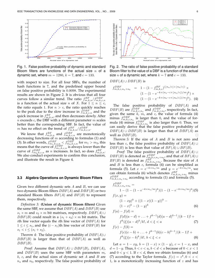
with respect to size. For all four SBFs, the number ofhash functions is 7, and the predefined upper boundon false positive probability is 0.0098. The experimentalresults are shown in Figure 2. It is obvious that all fourcurves follow a similar trend. The ratio fBF

m,k,n/fDBFm,k,c,n

is a function of the actual size n of X . For 1 ≤ n ≤ c,the ratio equals 1. For n > c, the ratio quickly reachesto the peak due to the slow increase in fDBF

m,k,c,n and thequick increase in fBF

m,k,n, and then decreases slowly. Aftern exceeds c, the DBF with a different parameter m scalesbetter than the corresponding SBF. In fact, the value ofm has no effect on the trend of fBF

m,k,n/fDBFm,k,c,n.

We know that fBFm,k,n and fDBF

m,k,c,n are monotonicallydecreasing functions of m according to formulas (1) and(3). In other words, fDBF

m1,k,c,n < fDBFm2,k,c,n for m1 > m2, this

means that the curve of fDBFm1,k,c,n is always lower than the

curve of fDBFm2,k,c,n as n increases. In fact, so does fBF

m,k,n.We also conduct experiments to confirm this conclusion,and illustrate the result in Figure 4.

3.3 Algebra Operations on Dynamic Bloom Filters

Given two different dynamic sets A and B, we can usetwo dynamic Bloom filters DBF (A) and DBF (B) or twostandard Bloom filters BF (A) and BF (B) to representthem, respectively.

Definition 3: (Union of dynamic Bloom filters) Giventhe same SBF, we assume that DBF (A) and DBF (B) uses1 ×m and s2 ×m bit matrixes, respectively. DBF (A) ∪DBF (B) could result in a (s1 + s2)×m bit matrix. Theith line vector equals the ith line vector of DBF (A) for1 ≤ i ≤ s1, and the (i− s1)th line vector of DBF (B) fors1 < i ≤ (s1 + s2).

Theorem 4: The false positive probability of DBF (A)∪DBF (B) is larger than that of DBF (A) as well asDBF (B).

Proof: Assume that DBF (A) ∪ DBF (B), DBF (A),and DBF (B) uses the same SBF with parameters m,k, c, and the actual sizes of dynamic set A and B arena and nb, respectively. The false positive probability of

0 200 400 600 800 1000 12000

5

10

15

20

25

Actual size of a dynamic set

The r

atio o

f fals

e pos

itive p

roba

bility

of st

anda

rdblo

om fil

ters

to tha

t of d

ynam

ic blo

om fil

ters

m=320,k=7m=640,k=7m=960,k=7m=1280,k=7

Fig. 2. The ratio of false positive probability of a standardBloom filter to the value of a DBF is a function of the actualsize n of a dynamic set, where k = 7 and c = 133.

DBF (A) ∪DBF (B) is

fDBFm,k,c,na+nb

= 1− (1− fBFm,k,c)

(bna/cc+bnb/cc) ×(1− (1− e−k×(na−c×bna/cc)/m)k)×(1− (1− e−k×(nb−c×bnb/cc)/m)k). (4)

The false positive probability of DBF (A) andDBF (B) are fDBF

m,k,c,naand fDBF

m,k,c,nb, respectively. In fact,

given the same k, m, and c, the value of formula (4)minus fDBF

m,k,c,nais larger than 0, and the value of for-

mula (4) minus fDBFm,k,c,nb

is also larger than 0. Thus, wecan easily derive that the false positive probability ofDBF (A) ∪ DBF (B) is larger than that of DBF (A) aswell as DBF (B).

Theorem 5: If the size of A and B is not zero andless than c, the false positive probability of DBF (A) ∪DBF (B) is less than that value of BF (A) ∪BF (B).

Proof: The false positive probability of DBF (A) ∪DBF (B) is denoted as fDBF

m,k,c,na+nb, and that of BF (A)∪

BF (B) is denoted as fBFm,k,na+nb

. Because the size of Aand B is less than c, formula (4) can be simplified asformula (5). Let x = e−k×na/m and y = e−k×nb/m, wecan obtain formula (6) which denotes fBF

m,k,na+nbminus

fDBFm,k,c,na+nb

according to formula (1) and formula (5).

fDBFm,k,c,na+nb

=

1− (1− (1− e−k×na/m)k)(1− (1− e−k×nb/m)k)(5)f(x, y) =

(1− xy)k + ((1− x)(1− y))k −(1− x)k − (1− y)k (6)

f(a)− f(d) =f(d)(a− d) + . . . + fk−1(d)(a− d)k−1/(k − 1)! +fk(ξ)(a− d)k/k!, d < ξ < a (7)

f(c)− f(b) =f(c)(c− b) + . . . + fk−1(b)(c− b)k−1/(k − 1)! +fk(ξ)(c− b)k/k!, b < ξ < c (8)

Let a = 1 − xy, b = (1 − x) × (1 − y), c = 1 − x, andd = 1−y. Thus, b < c < a, b < d < a because of 0 < x < 1and 0 < y < 1. If c < d, then we obtain formulas (6) and(7) according to the Taylor formula. f(z) = zk, 0 < z <1, is a monotonically increasing function of z and has


Fig. 3. False positive probability of BF (A)∪BF (B) minusthat of DBF (A) ∪ DBF (B) is a function of size na ofdynamic set A and nb of set B, where m = 1280, k = 7,and c = 133.a continuous k-rank derivative. The ith derivative is amonotonically increasing function for 1 < i ≤ k. It isobvious that a − D = c − b, d < c < a, b < d < a. Thus,each item of f(a) is larger than the corresponding itemof f(c), and so (6) is larger than 0. If c > d, the result isthe same. Theorem 5 is proved to be true.

On the other hand, we used MATLAB to calculate theresult of fBF

m,k,na+nbminus fDBF

m,k,c,na+nb. As shown in Fig-

ure 3, the false positive probability of DBF (A)∪DBF (B)is also less than that of BF (A)∪BF (B), even though thesize of A and B exceeds c.

3.4 Evaluations of Item Deletion Algorithm

3.4.1 Mathematical AnalysisAs mentioned above, multiple SBFs tend to allocateBfaddress(x) for an item x ∈ X in a DBF. It is clearthat only one SBF ever truly represented x during itsinput process; the other SBFs are false positives. Theitem deletion operation of DBF always omits such items,keeping their set membership information. The moti-vation is to prevent the DBF from producing potentialfalse negatives caused by an incorrect item deletion. Asa direct result of the item deletion operation, queries ofsuch items will yield false positives.

Recall that X has n items, and the DBF uses s = dn/ceSBFs. After the representation of X , we can consider theevent where a particular item x of X appears to be inmultiple SBFs. If x was represented by one of the first s−1 SBFs during the item insertion process, the probabilityof this event can be calculated by

f1(n) = 1− (1− fBFm,k,c)

s−2(1− fBFm,k,nl

). (9)

If item x was represented by the sth SBF during theitem insertion process, this event means that at least oneof the first s− 1 SBFs produce a false positive judgmentfor x, and the probability of this event can be calculatedby

f2(n) = 1− (1− fBFm,k,c)

s−1. (10)

It is easy to know that the value of formula (10) islarger than that of formula (9). We use formula (10) asan estimated upper bound on the probability that x of

0 500 1000 1500 2000 25000

0.1

0.2

0.3

0.4

0.5

0.6

0.7

0.8

0.9

1

Actual size nr of a dynamic set

False

posit

ive pr

obab

ility o

f dyn

amic

bloom

filter

m=640m=1280m=1920m=2560

Fig. 4. The false positive probability of four kinds of DBFsare functions of the actual size n of a dynamic set, wherek = 7, and the predefined threshold of false positiveprobability of each DBF is 0.0098.

X appears to be in multiple SBFs, and then achieve anestimated upper bound n×f2(n) on the number of suchitems which have more than one Bloom filter address.Our experimental results show that the real number isless than the estimated upper bound. If all items of X aredeleted, the DBF will try to perform the same operation.However, the DBF cannot guarantee deletion of all itemsdue to its special item deletion operation. In reality, theDBF still holds the membership information of at mostn × f2(n) items. If other items join X at the same timethat the original items are deleted, the DBF can reflectthe membership information of all items of X and atmost n × f2(n) remaining items. It is logical that thefalse positive probability of the DBF is always largerthan the theoretical value. Our experimental findingsshow similar results, and the difference between the realvalue and theoretical value is small. In other words, thenegative impact of the item deletion operation on a DBFcan be controlled at an accepted level.

3.4.2 Experimental AnalysisIn this section, we will first describe the implementationof k random and independent hash functions. Then, wewill compare the analytical model to the experimental re-sults for the number of items which have multiple Bloomfilter addresses. One critical factor in our experiments iscreating a group of k hash functions. In our experiments,they will be generated as

hi(x) =(g1(x) + i× g2(x)

)mod m. (11)

g1(x) and g2(x) are two independent and randomintegers in the universe with range {1, 2, . . . , m}. i rangesfrom 0 to k − 1. We use the SDBM MersenneTwistermethod to generate the two random integers for any itemx. Let the output of the SDBM Hash function as theseed of the random number generator (RNG) Mersen-neTwister. Then, the MersenneTwister will produce thetwo desired random integers. The SDBM hash functionseems to have a good over-all distribution for manydifferent sets. It also works well in situations where thereare high variations in the MSBs of the items in a set. TheMersenneTwister is capable of quickly producing very


0 200 400 600 800 1000 1200 14000

0.01

0.02

0.03

0.04

0.05

0.06

0.07

0.08

0.09

0.1

Actual size of a dynamic data set

The

ratio

r an

d th

e fa

lse

posi

tive

prob

abilit

yEstimated upperbound of rExperimental upperbound of rReal value of rDynamic bloom filter

Fig. 5. False positive probability of dynamic Bloom filtersand the percentage of data which has multiple Bloom filteraddresses, where m = 1280, k = 7, and c = 133.

TABLE 1Experimental upper bound and real value of r with

c = 133

n/c 2 3 4 5 6 7 8 9 10Upperbound 4 7 11 22 37 53 74 98 123

Real value 3 4 4 6 9 13 20 30 36

high-quality pseudo-random numbers. This mechanismrequires one hash function and one random numbergenerator to run k−1 rounds of (11) in order to generatea Bloom filter address Bfadddress(x) for item x. Itprovides a considerable amount of processing reductioncompared to using k actual hashes. Kirsch et al. showsthat this method does not increase the probability of falsepositives [29].

The multiple address problem causes some items toremain in a DBF even after they have been deleted fromset X . The ratio of the number of such items to thecardinality of set X is denoted as r. Recall that f2(n) isan estimated upper bound on r based on mathematicalanalysis. The experimental upper bound on r and realvalue of r are the average values achieved from 100rounds of simulations with different sets in each round.

Note that dynamic Bloom filters are designed to rep-resent many possible sets, and there are no benchmarksets in the field of Bloom filters. Our experiments donot seek particular sets but simply use names of files atsome peers in a peer-to-peer trace as the data source.The P2P trace is a snapshot of files that were shared byeDonkey peers between Dec 9, 2003 and Feb 2, 2004, andrecord 11014603 distinct files. We initialize ten sets withcardinality i × c for 1 ≤ i ≤ 10 using the trace data,and then implement ten DBFs. In our experiment, theparameters of each SBF are m = 1280, k = 7, and c = 133.For each DBF, the number of items possessing multipleBloom filter addresses from the corresponding set isdetermined, and then the experimental upper bound ofr is calculated. For each DBF, the item deletion algorithmmentioned above is performed, and the ratio of thenumber of remaining items to the original cardinalityof the corresponding set is the real value of r. Table 1shows the experimental results under different dynamicsets.

0 100 200 300 400 500 600 7000

0.005

0.01

0.015

0.02

0.025

0.03

0.035

0.04

0.045

0.05

Actual size of a dynamic data set

The

fals

e po

sitiv

e pr

obab

ility

Dynamic bloom filter, remain=0Dynamic bloom filter, remain=36Dynamic bloom filter, remain=20Dynamic bloom filter, remain=6

Fig. 6. False positive probability of dynamic Bloom filtersare functions of the actual size n of a dynamic set and theremaining data, where m = 1280, k = 7, and c = 133.

Figure 5 shows that the real value of r is less than theexperimental upper bound, the estimated upper boundand the false positive probability of a DBF. All fourcurves increase as the size of the dynamic set increases.The curve for the real value r increases smoothly andmaintains a low level when the real size of the set isless than ten times that of the estimated threshold. Onthe other hand, the frequency of deleting all items froma set and its corresponding DBF is often low, and theperiod is usually long.

Let’s consider the dynamic sets with n/c = 10, 8, 5. Wefirst delete all items of those sets based on the item dele-tion algorithm, and then continuously add new itemsto the set. It is easy to understand that the remainingitems can increase the false match probability of theDBF. Figure 6 shows that the more remaining items thereare, the greater the false positive probability will be. Inpractice, the frequency of deleting all items from a setand its corresponding DBF is very low; the false positiveprobability of a DBF is often larger than the expectedvalue, but still maintains a lower, more stable level. Onthe other hand, the real capacity of a DBF decreaseswith the number of those remaining items. Applicationscan use the change in the real capacity as a metric toevaluate the influence of the item deletion operation andto decide whether to represent the updated set again. Inthe future, we will seek a better method to solve themultiple address problem for an item.

3.5 Optimizations of Dynamic Bloom FiltersIn this subsection, we consider cases in which applica-tions do not require DBFs to provide the item deletionoperation. In those cases, DBFs use SBFs as a compo-nent and may be optimized from the following aspects.None of the optimization strategies proposed below aresuitable to other cases in which DBFs use CBFs as acomponent.

3.5.1 Improvement of Item Insertion OperationThe item insertion algorithm proposed previously couldbe optimized in two scenarios. First, sometimes it seemsto a new item of a normal set that it has been representedby a DBF, even if it is not. In this case, the new item is still


0 2 4 6 8 10 12 14 16 18 200

1

2

3

4

5

6

7

The value of s

The

val

ue o

f rat

io0.02

0.01

0.005

0.001

0.0005

0.0001

Fig. 7. The ratio of the number of items which haveat least one Bloom filter address before they are rep-resented to the threshold c is a function of s and thethreshold f .

inserted into an active SBF of the DBF. This kind of itemmay cause the DBF to allocate unnecessary SBFs. Second,duplicate insertions of an identical item in a multi-setdo not necessarily harm an SBF, but they may cause aDBF to extend unnecessarily [30]. Solving this issue re-quires a membership query before each insert; however,doing so increases the insertion complexity from k toO(k×s). Considering the additional computational costs,DBFs should only adopt the improved item insertionalgorithm if the previous Algorithm 1 causes at least oneunnecessary SBF.

As discussed in Section 3.4, n × f2(n) denotes anestimation of the number of items which have multipleBloom filter address after all items are represented,and are very similar to the experimental results. Theexperimental results, as well as the estimation, are largerthan the number of items which already have at least oneBloom filter address before they are represented in thetwo scenarios. Thus, the improved algorithm should beused only if

ratio =n× f2(n)

c≥ 1,

which implies that Algorithm 1 incurs at least one un-necessary SBF. The ratio is a monotonically increasingfunction of s and f which denotes an upper boundon the false match probability of an SBF. As shown inFigure 7, the value of ratio is always less than one iff ≤ 0.01, s ≤ 10 or f ≤ 0.001, s ≤ 20; hence, it isnot necessary to use the improved algorithm. Underother conditions, Algorithm 1 should be replaced by theimproved algorithm since the former causes at least oneunnecessary SBF.

The above discussions fail to consider the impact of amulti-set. If the distribution of duplicate items in a multi-set is known in advance, a multi-set could be treated asa normal set where those duplicate items act as identicalitems in a normal set, and could be analyzed in the sameway. Otherwise, we recommend adopting the improveditem insertion algorithm, which could be optimized bya better method of storing dynamic Bloom filters, asdiscussed below.

3.5.2 Compressed Dynamic Bloom FiltersIn some distributed applications, an SBF at a node isusually delivered to one or more nodes as a message.In this case, besides the three metrics of SBFs we haveseen so far, (1) the computational overhead of an itemquery operation, (2) the size of the filter in memory, and(3) the false match rate, a fourth metric can be used: thesize of a message used to transmit an SBF across the net-work. The compressed Bloom filters might significantlysave bandwidth at the cost of larger uncompressedfilters and some additional computation to compress anddecompress the filter sent across the network. In theidealized setting, using compression always reduces thefalse positive probability by adopting a larger Bloomfilter size and fewer hash functions than an SBF uses.Interested readers may obtain details concerning all ofthe theoretical and practical issues of compressed Bloomfilters in [18].

It is reasonable to compress a DBF by using com-pressed Bloom filters instead of SBFs. The compressedDBFs and MDDBFs could reduce both the transmissionsize and false positive probability of the uncompressedversions at the cost of larger memory and additionalcomputation overheads.

3.5.3 Approach for Storing Dynamic Bloom FiltersThere are two ways of storing a dynamic Bloom filterwith a set number of s SBFs. These are referred to asthe bit string and bit slice methods, respectively [31].The bit string approach stores the s SBFs dependentlyand sequentially. Instead of storing a DBF as an s × mlong bit strings, the bit slice method stores a DBF as anm × s long bit slices. We know that only a subset ofthe bit positions in each SBF need to be examined on aquery. One problem with the bit string approach is thatall s × m bits need to be retrieved on a query. For thebit slice approach, only a fraction of the bit slices needto be retrieved on a query.

4 PERFORMANCE EVALUATIONS

We use α to denote an upper bound on the false matchprobability of an SBF representing a static set with fixedcardinality n. Given α and n, the parameters k andm could be optimized for the SBF with m = dn ×log(α)/ log(0.61285)e and k = d(m/n) ln 2e. Given α andm, the capacity c can be optimized for the SBF withc = dm× log(0.61285)/ log(α)e. It is clear that the amountof memory allocated to an SBF increases linearly withn. SBF and its variations are practical approaches torepresent static sets; however, most applications oftenencounter dynamic sets without fixed cardinality besidesstatic sets. According to the structure of DBFs, we knowthat DBFs can represent dynamic sets as well as staticsets. In this section, we will first evaluate the perfor-mances of DBFs and SBFs in stand-alone applicationswith three different sets, and then discuss the distributedapplications of DBFs.


0 5 10 15 20 250

0.1

0.2

0.3

0.4

0.5

0.6

0.7

0.8

0.9

1

Ratio of actual size nr to designed size n

0 of a given dynamic set

Ratio

of st

anda

rd bl

oom

filter

size

to

dyna

mic b

loom

filter

size

Fig. 8. The ratio of size of a Bloom filter to that of a DBFis a function of a non-negative integer, which denotes theratio of n to c. The experimental condition is the same asthat in Figure 3.

4.1 Static Set with Fixed Cardinality

A dynamic set could be regarded as a series of staticsets over a sequence of discrete time. In this section,we use SBF and DBF to represent a dynamic set, andcompare them from two aspects at any given discretetime. The SBF is reconstructed according to its optimalconfiguration, as determined by the set cardinality.

For a dynamic set X , let s be dn/ce where n and cdenote the cardinality of X and capacity of SBF usedby DBF, respectively. For a DBF representing the set,formula of its false positive probability is simplifiedas formula (12). For an SBF representing that set, itcalculates how many bits it must consume in order toachieve the same false positive probability as the DBF.Finally, we establish the relationship between formulas(1) and (12), and achieve formula (13) to denote the ratioof the number of bits m1 used by an SBF to the numberof bits s×m used by a DBF.

fDBFm,k,c,n = 1− (1− (1− e−k×c/m)k)dn/ce (12)

m1

s×m=

−k × c

m× ln(1− k√

1− (1− y)s)(13)

The following conclusions can be drawn from formula(13) and Figure 8. To obtain the same false match prob-ability, SBF and DBF use the same bits to represent X ifn ≤ c. However, the SBF consumes fewer bits than theDBF if n > c. The difference of bits used by DBF andSBF is small if s is not too large.

Let us compare the false positive probability of anSBF and a DBF which use the same bits to representan identical dynamic set. That is, an SBF is allowedto expand its size to s × m and to re-represent thedynamic set as the set cardinality grows. In this case, thestandard Bloom filter is defined as NBF. The false matchprobability of an SBF could be calculated according to(1). The false match probability of a DBF should still be(3). It is necessary to compare fDBF

m,k,c,n and fNBFm,k,c,n under

this situation, and we have

fNBFm,k,c,n = (1− e−k×n/(m×dn/ce))k (14)

0 200 400 600 800 1000 1200 14000

0.01

0.02

0.03

0.04

0.05

0.06

0.07

0.08

0.09

0.1

Actual size nr of a dynamic set.

The f

alse p

ositiv

e prob

abilit

y

Dynamic bloom filterStandard bloom filter

Fig. 9. False positive probability of dynamic and standardBloom filters are functions of the actual size of a dynamicset. Standard Bloom filters can expand the filter size m todn/ce ×m. m = 1280, k = 7, and c = 133.

The experimental results are shown in Figure 9. Weconclude that fDBF

m,k,c,n = fNBFm,k,c,n ≤ fBF

m,k,c for n ≤ c. Forn > c, fDBF

m,k,c,n grows as the set cardinality increases,and fNBF

m,k,c,n fluctuates between i× c and (i + 1)c, wherei is any non-negative integer. Let nx < c be any non-negative integer, thus fNBF

m,k,c,nx+(i−1)×c is not larger thanfNBF

m,k,c,nx+i×c. In fact, fNBFm,k,c,n grows as the set cardinality

increases in the whole range, but the increase rate isslower than that of fDBF

m,k,c,n.In summary, to achieve the same false match probabil-

ity, an SBF never uses more bits than a DBF to representany static version of that dynamic set if the SBF isactively reconstructed as the increase of set cardinality. Itis clear that the SBF produces large, even huge, overheaddue to frequent reconstructions. On the contrary, a DBFis not required to be reconstructed if its false matchprobability is controlled at an acceptable level with theincrease of set cardinality. Note that the false matchprobability of a DBF might sometimes become too largeto be tolerated by many applications. It is necessary tooccasionally reconstruct the DBF. In the next subsection,we will compare DBFs and SBFs in the whole lifetime ofa dynamic set instead of comparing them in a series ofdiscrete time.

4.2 Dynamic Set with an Upper Bound on Set Cardi-nalityIn this section, we use SBF as well as DBF to represent adynamic set X with an upper bound N on set cardinality.Let α denote the upper bound on false match probabilityof the SBF as well as DBF. In many applications, thedistribution of set cardinality covers a large range [32],[33]. In such a distribution, the upper bound is some-times several orders of magnitude larger than the meanor minimum cardinality. Applications usually allocatea large number of bits for an SBF at the outset withm = dN × log(α)/log(0.61285)e. These bits are largeenough for the SBF to accommodate all possible items ofX , while decreasing the space-efficiency of the SBF. DBF,however, allocates enough bits in an incremental and on-demand fashion. A common objective of SBF and DBFis to guarantee that the false match probability never


2 4 6 8 10 12 14 16 18 206000

6500

7000

7500

8000

8500

9000

9500

10000

10500

11000

Number of SBFs in a DBF

Exp

ecte

d m

emor

y si

ze (#

of b

its)

Uniform distribution

Normal distribution

Random zipf distribution

Maximum zipf distribution

Minimum zipf distribution

Fig. 10. The memory size of a DBF under different setcardinality distributions: a uniform distribution, a normaldistribution with u = dN/2e and σ2 = 20, and a Zipfdistribution with 0.4 as parameter, where N=1330 andα=0.0098.exceeds the α and to make sure that they are not requiredto be reconstructed as the set cardinality changes.

We now address the problem of designing a minimumsize DBF when the probability density function of the setcardinality is known. We assume that s homogeneousSBFs make up the DBF, and δ denotes the upper boundon the false match probability of each SBF. The overallfalse match probability α for the DBF has to be appor-tioned among the individual SBFs. According to formula(3), we know that α = 1 − (1 − δ)s. As a result, we canderive the value of parameter δ with δ = 1− (1− α)1/s.

The capacity of the DBF is N since at most N itemsof the set are accommodated by it. Since the N itemsare allocated to a certain number of s SBFs evenly, thecapacity of the ith SBF is defined as ci = dN/se for 1 ≤i ≤ s. In order to solve this problem, we must determinethe parameters m, k, δ and s such that the false matchprobability DBF never exceeds the upper bound α.

Let pi represent the probability that X has i itemswhere 1 ≤ i ≤ N , i.e.,

∑Ni=1 pi = 1. We associate

the ith SBF of the DBF with a ri which implies anupper bound on the probability that this SBF is used.Let r1 = 1 and ri =

∑Nj=c×(i−1)+1 pj for i = 2, 3, ..., s,

where c denotes the capacity of any SBF. The expectednumber of bits used by the DBF is upper bounded by∑s

i=1 m× ri. Recall that the bits used by each SBF is m =d(N/s)× log(δ)/ log(0.6185))e. We formulate the problemto minimize

∑si=1 ri × (N/s)× log(δ)/ log(0.6185).

Minimize∑s

i=1ri × (N/s)× log(δ)/ log(0.6185)

Subject toδ = 1− (1− α)1/s

s > 0

The optimized value of parameter s could be derivedfrom the solution of this optimization problem. Oncewe have s, it can be used to calculate the false matchprobability δ and capacity c for these homogeneous SBFs,and then determine the parameters m and k accordingto the design method of an SBF. The set cardinalitydistribution has a direct impact on the result of this opti-mization problem. We compare the minimized memory

size of a DBF under five different cardinality distribu-tions through experiments: normal distribution, uniformdistribution, random Zipf distribution, minimum Zipfdistribution, and maximum Zipf distribution.

The first two distributions have been widely usedfor generating synthetic sets to emulate real sets [34].In many networking applications, it is observed thatthe set cardinality at each node conforms to a Zipfdistribution with a long tail. There is a bijective mappingfrom the cardinality values to the rank values. The Zipfdistribution is called random if any rank value is mappedto a random integer over a range {1, ..., N} uniformly.It is called minimum if the largest and second largestcardinality values are mapped to the last and secondlast ranks respectively, and so on. It is called maximumif the largest and second largest cardinality values aremapped to the first and second ranks respectively, andso on.

As shown in Figure 10, all five curves follow a similartrend as s increases under the constraints that N=1330and α=0.0098. The expected memory size of each curvefirst decreases as s grows, and then increases after thes exceeds one or more keen points on the whole. It isclear that the expected memory size under the maximumZipf distribution is always larger than that under otherdistributions of the same value of s. The reason is thatthe ri under the maximum Zipf distribution is greaterthan that under other distributions for 2 ≤ i ≤ s and anygiven value of s. For each curve of DBF, the minimummemory size is achieved when the value of s is equalto a keen point on the curve, and is less than that of anSBF under the same constraints.

We then evaluate the impact of set cardinality on theminimum memory size of the SBF and the five differentDBFs where α=0.0098. Figure 11 shows that a DBF withrandom Zipf distribution uses almost the same amountof memory as a DBF with uniform distribution, whileDBFs with maximum and minimum Zipf distributionsconsume the most and least memory among the fiveDBFs, respectively. All DBFs, however, consistently out-perform SBFs independent of set cardinality, and theperformance difference seems to widen as set cardinalityincreases. In experiments, we also focus on the influenceof set cardinality on the ratio of memory size of DBFto that of SBF. As shown in Figure 12, DBFs withmaximum Zipf distribution, random Zipf distribution,normal distribution, and minimum Zipf distribution cansave about 5%, 19%, 20%, and 35% of the memory usedby SBF, respectively. The experimental results show thatthe set cardinality has a trivial impact on the ratio of thememory size of DBF to that of SBF, while the cardinalitydistributions have a major impact on that metric.

Moreover, we evaluate the impact of false match prob-ability on the minimum memory size of SBF and the fivedifferent DBFs where N=13300. Figure 11 shows thatDBFs with maximum and minimum Zipf distributionsconsume the most and least memory among the fiveDBFs, respectively. The five DBFs, however, consistently


0 1 2 3 4 5 6 7 8 9 10

x 105

0

1

2

3

4

5

6

7

8

9

10x 10

6

Upper bound on set cardinality

Min

imum

mem

ory

size

(#o

f bi

ts)

SBF

DBF with uniform distribution

DBF with normal distribution

DBF with random zipf distribution

DBF with maximum zipf distribution

DBF with minimum zipf distribution

Fig. 11. Memory size under different values of set cardi-nality.

0 1 2 3 4 5 6 7 8 9 10

x 105

0.65

0.7

0.75

0.8

0.85

0.9

0.95

1

Upper bound on set cardinality

Rat

io o

f min

imum

mem

ory

of D

BF

to th

at o

f SB

F






Fig. 12. Ratio of memory size of DBF to that of SBF underdifferent set cardinality distributions.

outperform SBFs independent of false match probability.In experiments, we also focus on the influence of thefalse match probability on the memory size of DBF, andthe ratio of memory size of DBF to that of SBF. As shownin Figure 13, for each DBF, the memory size decreases asthe false match probability increases. As shown in Figure14, for each DBF, the ratio increases as the false matchprobability increases; however, it will always be less than1 when the false match probability is not larger than 5%.Actually, the ratio for each DBF will reach, at most, 1when the false match probability exceeds 5%. That is,the five DBFs never consume more memory than SBF,and save more memory as the false match probabilitydecreases.

Figure 15 shows the impact of the Zipf parameter onmemory size under different Zipf distributions2 whereN=1330 and α=0.0098. We observe that DBFs with aminimum Zipf distribution perform better as the pa-rameter value increases, and DBFs with a random Zipfdistribution outperform SBFs almost independent of theZipf parameter value. If the Zipf parameter is less than0.6, DBFs with a maximum Zipf distribution also out-perform SBFs, otherwise, they perform worse than SBFs.Figure 16 shows the impact of standard deviation σ onthe memory size of DBFs with normal distribution. Weobserve that DBFs with normal distribution use morememory as the value of σ increases, however, they

2. A large Zipf parameter means that the frequencies of somecardinality values are much higher than others. A small Zipf parametermeans that the frequency of each cardinality value occurs just as often

0.0000001 0.000001 0.00001 0.0001 0.001 0.01 0.10.5

1

1.5

2

2.5

3

3.5

4

4.5x 10

5

False match probability

Min

imum

mem

ory

size

(#o

f bits

)

SBF






Fig. 13. Memory size under different false match proba-bilities.

0.0000001 0.000001 0.00001 0.0001 0.001 0.01 0.1 0.2 0.4 0.50.4

0.5

0.6

0.7

0.8

0.9

1

1.1

False match probability

Exp

ecte

d m

emor

y si

ze (#

of b

its)






Fig. 14. Ratio of memory size of DBF to that of SBF underdifferent false match probabilities.

always outperform SBFs.

4.3 Dynamic Set without an Upper Bound on SetCardinality

In this section, we consider another scenario in which ap-plications do not know the upper bound N in advance.Let β and γ denote the left and right upper bounds onthe false match probability with β < γ. In this scenario,applications use a pair of β and γ instead of a tight upperbound α. In reality, applications expect the false matchprobability is less than β, and also tolerate an event thatthe false match probability is sometimes greater than βbut less than γ. A common objective of DBF and SBF is toguarantee that the false match probability never exceedsγ as the set cardinality changes. In order to satisfy thisobjective, the DBF and the SBF may be reconstructed asthe cardinality changes.

For a dynamic set, applications usually estimate athreshold n0 of the set cardinality and use an initialSBF to represent the dynamic set. In practice, it is verydifficult to estimate n0 in an accurate manner. Onepossible approach is to trace the change of a dynamicdata set, and then to investigate the statistic metric ofset size before using DBF to represent that data set.The parameters m and k for an SBF are initialized withm=dn0 × log(β)/ log(0.61285)e and k=d(m/n0) ln 2e. Asshown in Figure 1, the false match probability exceeds βdramatically when the set cardinality exceeds n0 grad-ually. Moreover, the false match probability exceeds γonce the set cardinality is greater than n0× log(β−γ). To


0 0.5 1 1.5 2 2.5 3 3.5 4 4.5 50

5000

10000

15000

Zipf parameter

Min

imum

mem

ory

size

(#of

bits

)

SBF




Fig. 15. Impact of Zipf parameter on minimum memorysizehandle this issue, n0 is assigned a new value which is atleast greater than n0× log(β−γ), and then the initial SBFis reconstructed using new parameters to represent thedynamic set again. There exist many policies to enlargethe value of n0. This paper does not discuss this in detailsince different policies have less impact on the finalresults. If the false match probability exceeds γ again,the SBF is adjusted in the same way.

DBF first adopts an SBF to represent the dynamic set,and may expand its capacity by allocating more SBFs asthe set cardinality increases. As shown in Figure 1, thefalse match probability of DBF increases slower than SBFwhen the set cardinality gradually exceeds c. The falsematch probability exceeds γ once the set cardinality isgreater than n0 × dlog(1 − γ)/ log(1 − β)e. To deal withthis issue, c is reassigned a new value which is at leastgreater than n0 × dlog(1 − γ)/ log(1 − β)e, and the DBFis reconstructed to represent the dynamic set again. Thispaper does not discuss policies to enlarge n0 in detail forsimilar reasons. If the false match probability of a newDBF exceeds γ again, the DBF must be adjusted in thesame way.

In reality, it is unavoidable to reconstruct DBFs andSBFs under specific conditions if the upper bound onset cardinality is not known a priori. Fortunately, theadjustment frequency of DBF is lower than that of SBF,especially when the difference between β and γ is large;that is, DBF causes less overhead and is more stable thanSBF due to infrequent reconstructions as the increase ofset cardinality. Note that if the difference between β andγ is very low, the benefit of our approach using leftand right bounds on the false match probability becomestrivial. To address this rare case, we use the approachesproposed in Section 4.2 after estimating the cardinalitydistribution and initializing N=n0 and α=γ.

4.4 Distributed Application Scenarios

In the above discussions, we considered SBF and DBF asobjects residing in memory in stand-alone applications.In distributed applications, however, they are not justobjects that reside in memory, but objects that mustbe transferred between nodes. In this case, all nodesare required to adopt the same configuration of m, k,and hash functions in order to guarantee compatibility

2 4 6 8 10 12 14 16 18 200.9

0.95

1

1.05

1.1

1.15

1.2

1.25

1.3x 10

5

Normal distribution parameter sigma

Min

imum

mem

ory

size

(#of

bits

)

SBF


Fig. 16. Impact of standard deviation σ on minimummemory size

and interoperability of SBF or DBF between any pair ofnodes.

We first consider the case in which the upper boundsN and α on the set size and false match probabilityover nodes, depending on the applications, are known apriori. Nodes can construct a local but homogeneous SBFwith m=dN × log(α)/ log(0.61285)e and k=d(m/N) ln 2eeven if those sets are different in size. This approachrequires the nodes with small sets to sacrifice more spaceto be in accordance with those nodes with the largesets, hence hurting the space-efficiency and causing largetransmission overhead. As discussed in Section 4.2, DBFcan address this drawback of SBF if the distribution ofset sizes over nodes is known by the relevant applica-tion. The reason is that each node allocates just enoughmemory to a DBF according to its set size, and can satisfythe requirement of compatibility and inter-operability ofDBF with other nodes. Although the approaches pro-posed in Section 4.2 focus on stand-alone applications,they are also suitable to distributed applications. Theonly difference is that the expected number of bits usedby a DBF is minimized in stand-alone applications, whilethe total number of bits used by DBFs at all nodes is min-imized in distributed applications. For more information,we refer the reader to Section 4.2.

We then consider the case in which the upper boundon set sizes over nodes is not known in advance. Inthis scenario, as discussed in Section 4.3, applicationsimpose β and γ (β < γ) as a pair of upper boundson the false match probability over nodes, and estimatea threshold n0 on the upper bound on set sizes overnodes. If applications use SBFs to represent sets overnodes, an event where the size of the set at any nodeexceeds n0 × log(β − γ), will trigger a reconfigurationof its SBF, thereby propagating a new configuration toother nodes, and reconstructing an SBF at each node.It is clear that frequent reconfigurations lead to hugeoverhead and destroy the stability of applications. Onepossible solution to this problem is to overestimate n0

and allocate a larger SBF at each node. This solution,however, hurts the space-efficiency of SBF and causeslarge transmission overhead. If applications use DBFsinstead of SBFs, all nodes reconfigure their DBFs only ifthe set size at any node exceeds n0×dlog(1−γ)/ log(1−


β)e. Note that the node just expands its DBF withoutperforming the consistency operation over all nodes ifits set size is greater than n0 × log(β − γ) but less thann0×dlog(1−γ)/ log(1−β)e. It is clear that the adjustmentfrequency of DBF is lower than that of SBF especiallywhen the difference between β and γ is large. DBFs aremore stable than SBFs with the increase of set cardinalityin this case. For more information, we refer the readerto Section 4.3.

After discussing the use of approaches of DBF, weconsider a necessary procedure to update a DBF indistributed applications. For each DBF, we adopt an in-cremental update procedure by only sending those SBFswhich are changed. For each varied SBF, the procedureto send updates first inspects if an old version of the SBFexists in the previous DBF. If not, this must be an addedSBF and the update is simply the SBF itself. Otherwise,an update is sent by computing the xor of the currentversion with the previous version. All updates can becompressed using arithmetic coding before being sentreliably. At the other end, the procedure to receive eachupdated SBF first inspects if a previous SBF exists. If not,this must be an added new SBF and the update is simplystored in the corresponding DBF. Otherwise, the updatedSBF is treated as an incremental one and its previous SBFis modified suitably by computing its bitwise xor withthe new update.

5 CONCLUSION

A Bloom filter is an excellent data structure for succinctlyrepresenting static sets with fixed cardinality in order tosupport membership queries. However, it does not takedynamic sets into account. In reality, most applicationsoften encounter dynamic data sets as well as static sets.We present dynamic Bloom filters to deal with dynamicsets as well as static sets. Dynamic Bloom filters notonly inherit the advantage of Bloom filters, but alsohave better features than Bloom filters when dealingwith dynamic sets. The false match probability of Bloomfilters increases exponentially with the increase of thecardinality of a dynamic set, while that of dynamicBloom filters increases slowly because it expands ca-pacity in an incremental manner according to the setcardinality.

Through comprehensive mathematical analysis, weshow that dynamic Bloom filters use less expected mem-ory than Bloom filters when dealing with dynamic setswith upper bounds on set cardinality, and that dynamicBloom filters are more stable than Bloom filters due toinfrequent reconstruction when addressing dynamic setswithout upper bounds on set cardinality. Moreover, theanalytical results hold in stand-alone applications as wellas distributed applications. The only disadvantage is thatdynamic Bloom filters do not outperform Bloom filtersin terms of false match probability when dealing with astatic set with the same size memory.

ACKNOWLEDGMENTS

The authors would like to thank Maria Basta and Chris-tian Esteve for their constructive comments and carefulproofreading. The work of Deke Guo was supported inpart by the Ph.D. Candidates Research Foundation ofNational University of Defense Technology under GrantNo. 0615. The work of Jie Wu was supported in part byNSF grants CNS 0422762, CNS 0434533, CNS 0531410,and CNS 0626240.

REFERENCES

[1] B. Bloom. Space/time tradeoffs in hash coding with allowableerrors. Commun. ACM, 13(7):422–426, 1970.

[2] J. K. Mullin. Optimal semijoins for distributed database systems.IEEE Trans. Software Eng., 16(5):558–560, 1990.

[3] L. F. Mackert and G. M. Lohman. R* optimizer validation andperformance evaluation for distributed queries. In Proc. the 12thInternational Conference on Very Large Data Bases (VLDB), pages 149–159, Kyoto, Jpn, August 1986.

[4] A. Broder and M. Mitzenmacher. Network applications of bloomfilters: A survey. Internet Mathematics, 1(4):485–509, 2005.

[5] J. Kubiatowicz, D. Bindel, Y. Chen, S. Czerwinski, P. Eaton, andD. Geels. Oceanstore: An architecture for global-scale persistentstorage. ACM SIGPLAN Notices.

[6] J. Li, J. Taylor, L. Serban, and M.Seltzer. Self-organization in peer-to-peer system. In Proc. the 10th ACM SIGOPS European Workshop,Saint-Emilion, France, September 2002.

[7] F. M. Cuena-Acuna, C. Peery, R. P. Martin, and T. D. Nguyen.Plantp: Using gossiping to build content addressable peer-to-peer information sharing communities. In Proc. the 12th IEEEInternational Symposium on High Performance Distributed Computing,pages 236–249, Seattle, WA, USA, June 2003.

[8] S. C. Rhea and J. Kubiatowicz. Probabilistic location and routing.In Proc. IEEE INFOCOM, pages 1248–1257, New York, NY, UnitedStates, June 2004.

[9] T. D. Hodes, S. E. Czerwinski, and B. Y. Zhao. An architecture forsecure wide-area service discovery. Wireless Networks, 8(2-3):213–230, 2002.

[10] P. Reynolds and A. Vahdat. Efficient peer-to-peer keywordsearching. In Proc. ACM International Middleware Conference, pages21–40, Rio de Janeiro, Brazil, June 2003.

[11] D. Bauer, P. Hurley, R. Pletka, and M. Waldvogel. Bringingefficient advanced queries to distributed hash tables. In Proc.IEEE Conference on Local Computer Networks, pages 6–14, Tampa,FL, United States, November 2004.

[12] L. Fan, P. Cao, J. Almeida, and A. Broder. Summary cache: Ascalable wide-area web cache sharing protocol. IEEE/ACM Trans.Networking, 8(3):281–293, 2000.

[13] C. D. Peter and M. Panagiotis. Bloom filters in probabilisticverification. In Proc. the 5th International Conference on FormalMethods in Computer-Aided Design, pages 367–381, Austin, Texas,USA, November 2004.

[14] C. Jin, W. Qian, and A. Zhou. Analysis and management ofstreaming data: A survey. Journal of Software, 15(8):1172–1181, 2004.

[15] F. Deng and D. Rafiei. Approximately detecting duplicates forstreaming data using stable bloom filters. In Proc. 25th ACMInternational Conference on Management of Data (SIGMOD), pages25–36, Chicago, Illinois, USA, June 2006.

[16] F. Bonomi, M. Mitzenmacher, R. Panigrahy, S. Singh, andG. Varghese. Beyond bloom filters: From approximate membershipchecks to approximate state machines. In Proc. ACM SIGCOMM,pages 315–326, Pisa, Italy, September 2006.

[17] K. Li and Z. Zhong. Fast statistical spam filter by approximateclassifications. In Proc. the Joint International Conference on Measure-ment and Modeling of Computer Systems, SIGMETRICS/Performance,pages 347–358, Saint Malo, France, June 2006.

[18] M. Mitzenmacher. Compressed bloom filters. IEEE/ACM Trans.Networking, 10(5):604–612, 2002.

[19] A. Kirsch and M. Mitzenmacher. Distance-sensitive bloom filters.In Proc. the 8th Workshop on Algorithm Engineering and Experiments(ALENEX06), Miami, Florida,USA, January 2006.


[20] A. Kirsch and M. Mitzenmacher. Building a better bloom filter.tr-02-05.pdf, January 2006.

[21] A. Kumar, J. Xu, J. Wang, O. Spatschek, and L. Li. Space-codebloom filter for efficient per-flow traffic measurement. In Proc.23rd IEEE INFOCOM, pages 1762–1773, Hongkong, China, March2004.

[22] S. Cohen and Y. Matias. Spectral bloom filters. In Proc. 22nd ACMInternational Conference on Management of Data (SIGMOD), pages241–252, San Diego, CA, United States, June 2003.

[23] R. P. Laufer, P. B. Velloso, and O. C. M. B. Duarte. Generalizedbloom filters. Technical Report Research Report GTA-05-43, Uni-versity of California, Los Angeles (UCLA), September 2005.

[24] B. Chazelle, J. Kilian, R. Rubinfeld, and A. Tal. The bloomier filter:an efficient data structure for static support lookup tables. In Proc.5th Annual ACM-SIAM Symposium on Discrete Algorithms (SODA),pages 30–39, New Orleans, Louisiana, USA, January 2004.

[25] F. Hao, M. Kodialam, and T. V. Lakshman. Building highaccuracy bloom filters using partitioned hashing. In Proc. SIG-METRICS/Performance, pages 277–287, San Diego, CA, USA, June2007.

[26] D. Guo, J. Wu, H. Chen, and X. Luo. Theory and network ap-plications of dynamic bloom filters. In Proc. 25th IEEE INFOCOM,Barcelona, Spain, April 2006.

[27] M. Xiao, Y. Dai, and X. Li. Split bloom filters. Chinese Journal ofElectronic, 32(2):241–245, 2004.

[28] P. S. Almeida, C. Baquero, N. M. Preguica, and D. Hutchison.Scalable bloom filters. Inf. Process. Lett., 101(6):255–261, 2007.

[29] A. Kirsch and M. Mitzenmacher. Less hashing, same performance:Building a better bloom filter. In Proc. the 14th Annual Euro-pean Symposium on Algorithms (ESA 2006), pages 456–467, Zurich,Switzerland, September 2006.

[30] J. Wang, M. Xiao, J. Jiang, and B. Min. I-dbf: an improved bloomfilter representation method on dynamic set. In Fifth InternationalConference on Grid and Cooperative Computing Workshops, pages 156–162, Changsha, China, September 2006.

[31] A. Kent and R. S. Davis. A signature file scheme based on multipleorganizations for indexing very large text databases. Journal of theAmerican Society for Information Science, 41(7):508–534, 1990.

[32] M. Faloutsos C. Faloutsos and P. Faloutsos. On power-lawrelationships of the internet topology. In Proc. ACM SIGCOMM,pages 251 – 262, Cambridge, Massachusetts, United States, August1999.

[33] F. Hao, M. Kodialam, and T. V. Lakshman. Incremental bloomfilters. In Proc. IEEE INFOCOM, Phoenix, Arizona, United States,2008.

[34] S. Melnik and H. C. Molina. Adaptive algorithms for set contain-ment joins. ACM Transactions on Database Systems, 28:56–99, 2003.

Deke Guo received the B.E. degree in industryengineering from Beijing University of Aeronau-tic and Astronautic, Beijing, China, in 2001, andthe Ph.D. degree in management science andengineering from National University of DefenseTechnology, Changsha, China, in 2008. He wasa visiting scholar in the Department of ComputerScience and Engineering, Hong Kong Universityof Science and Technology from Jan. 2007 toJan. 2009. Currently, he is an assistant professorof Information System and Management, Na-

tional University of Defense Technology, Changsha, China. His currentresearch focus on peer-to-peer networks, Bloom filters, MIMO, data cen-ter networking, wireless sensor networks, and wireless mesh networks.He is a member of the ACM and the IEEE.

Jie Wu is currently a distinguished professor inthe Department of Computer Science and Engi-neering, Florida Atlantic University. He has beenon the editorial board of the IEEE Transactionson Parallel and Distributed Systems and was aguest editor of Computer and the Journal of Par-allel and Distributed Computing. He is currentlyon the editorial board of the IEEE Transactionson Mobile Computing. He was a program cochairof the First IEEE International Conference onMobile Ad Hoc and Sensory Systems (MASS

2004), the executive program vice chair of the 28th IEEE InternationalConference on Distributed Computing Systems (ICDCS 2008), and theprogram vice chair of the 29th International Conference on ParallelProcessing (ICPP 2000). He was also the general chair of MASS2006 and is the general chair of the 22nd IEEE International Paralleland Distributed Processing Symposium (IPDPS 2008). He has servedas a distinguished visitor of the IEEE Computer Society and is thechairman of the IEEE Technical Committee on Distributed Processing(TCDP). His research interests include wireless networks and mobilecomputing, routing protocols, fault-tolerant computing, and intercon-nection networks. He has published more than 450 papers in variousjournals and conference proceedings. He is the author of DistributedSystem Design (CRC Press). He is the recipient of the 1996-1997,2001-2002, and 2006-2007 Researcher of the Year Awards from FloridaAtlantic University. He is a fellow of the IEEE.

Honghui Chen received the M.S. degree inoperational research and the Ph.D. degree inmanagement science and engineering from Na-tional University of Defense Technology, Chang-sha, China, in 1994 and 2007, respectively.Currently, he is a professor of Information Sys-tem and Management, National University ofDefense Technology, Changsha, China. His re-search interests are requirement engineering,web services, information grid, and peer-to-peernetworks. He has co-authored three books in the

past five years.

Ye Yuan Ye Yuan received the B.S. and M.S.degrees in computer science from NortheasternUniversity, China, in 2004 and 2007, respec-tively. Currently, he is a Ph.D. candidate in theDepartment of Computer Science, Northeast-ern University. He is also a visiting scholar inthe Department of Computer Science and En-gineering, Hong Kong University of Science andTechnology. His current research focus on peer-to-peer computing, graph databases, uncertaindatabase, probabilistic database, and wireless

sensor networks.

Xueshan Luo received the B.E. degree in in-formation engineering from Huazhong Instituteof Technology, Wuhan, China, in 1985, theM.S. and Ph.D. degrees in system engineer-ing from National University of Defense Tech-nology, Changsha, China, in 1988 and 1992,respectively. He was a faculty member and asso-ciate professor at National University of DefenseTechnology from 1992 to 1994 and from 1995 to1998, respectively. Currently, he is a professor ofInformation System and Management, National

University of Defense Technology. His research interests are in thegeneral areas of information system and operation research. His currentresearch focuses on architecture of information system.

IEEE TRANSACTIONS ON KNOWLEDGE AND DATA …

Documents

Transcript of IEEE TRANSACTIONS ON KNOWLEDGE AND DATA …