IEEE TRANSACTIONS ON EVOLUTIONARY COMPUTATION, …khaos.uma.es/jmgn/tesis/papers/paperTEC.pdf ·...
17
IEEE TRANSACTIONS ON EVOLUTIONARY COMPUTATION, VOL. X, NO. Y, JANUARY ZZZZ 1 Optimal Cycle Program of Traffic Lights with Particle Swarm Optimization Jos´ e Garc´ ıa-Nieto, Ana Carolina Olivera, and Enrique Alba Abstract—Optimal staging of traffic lights, and in particular optimal light cycle programs, is a crucial task in present day cities with potential benefits in terms of energy consumption, traffic flow management, pedestrian safety, and environmental issues. Nevertheless, very few publications in the current literature tackle this problem by means of automatic intelligent systems, and, when do so, are focused to limited areas with elementary traffic light schedules. In this paper, we propose an optimization approach in which a Particle Swarm Optimizer (PSO) can find successful cycle programs of traffic lights. The solutions obtained are simulated with SUMO, a well-known microscopic traffic simulator. In this study, we have tested two large and heterogeneous metropolitan areas with hundreds of traffic lights located in the cities of Bah´ ıa Blanca in Argentina (American style), and M´ alaga in Spain (European style). Our algorithm is shown to obtain efficient cycle programs of traffic lights for both kinds of cities. In comparison with expertly predefined cycle programs (close to real ones), our PSO achieved quantitative improvements for the two main objectives: the number of vehicles that reach their destinations and the global trip time 1 . Index Terms—Programming Cycles of Traffic Lights, Particle Swarm Optimization, SUMO Simulator of Urban MObility. I. I NTRODUCTION P OLLUTION, congestion, security, parking, and many other problems derived from vehicular traffic are present every day in most cities around the world. Since changes in urban area infrastructure are usually not possible, researchers often agree in that a correct staging of traffic lights can help to reduce these problems by improving the flow of vehicles through the cities [33], [41], [43]. Nevertheless, as traffic lights are installed in cities and their number grows, their joint programming becomes more complex due to the huge number of combinations that appear, and hence, the necessity of implementing automatic systems to optimally program the cycles of traffic lights is beyond doubt. In this sense, current research efforts in the field of auto- matic traffic control signals are directed to two main initiatives: on the one hand, automatic models of adaptation of signal control are designed [7], [20], [51] to change cycle programs durations in every moment of the day as vehicles in queues Jos´ e Garc´ ıa-Nieto and Enrique Alba are with Dept. Lenguajes y Ciencias de la Computaci´ on, University of M´ alaga, Campus de Teatinos, 29071, M´ alaga-Spain. E-mail: [email protected], [email protected] Ana Carolina Olivera is with Departamento de Ciencias e Ingenier´ ıa de la Computaci´ on, Universidad Nacional del Sur, Av. Alem 1253, 8000, Bah´ ıa Blanca-Argentina. E-mail: [email protected] 1 All the material generated in the experimentation: software, scenario instances, scripts, cycle programs, traces, figures, etc., is available online in http//neo.lcc.uma.es/problems/traffic-lights. demand those changes. The operation of these kind of tools is directly related to the sensor system and real time com- putation of the traffic flow in real time. Although these tools demonstrate a successful performance in several cities around the world [7], [5], the real management of the traffic network has a high cost of operation and the “real world” generally tends to repeat traffic flow patterns (rush hour, holidays, etc.). On the other hand, modern simulators [21], [24], [32] are very useful in helping the traffic management, since they provide researchers with an immediate and continuous source of information about traffic flow. In addition, economical issues are also taken into account in these kinds of researches, since the use of real traffic tests implies the necessity of additional staff and sensoring platforms. Many studies in traffic flow simulation have been performed representing both macro- scopic [33] and microscopic [41], [46] traffic views. In the last few years, efforts have been concentrated on combining an accurate microscopic modeling of traffic flow [24], [41] and the programming of convenient cycles of traffic lights [35]. In this sense, the use of intelligent methods have demonstrated their usefulness to the optimization of programming cycles of traffic lights [4], [41]. However, authors in general have addressed specific urban areas with few intersections and a small number of traffic lights (from 1 to 4 intersections with around 2 traffic lights controlling each intersection) [8], and most of them consist on ad-hoc algorithms designed only for one specific instance [4], [41]. The use of intelligent techniques for large and heterogeneous cases of study is still an open issue [29]. It is a complex problem since the greater the number of adjacent intersections, the higher the interaction between the traffic lights (which increases the complexity of the problem by introducing a high epistasis between variables). All this motivated us to propose a technique based on a Particle Swarm Optimizer [13], [11], [25] that will be shown to find successful cycle programs of traffic lights coupled with SUMO (Simulator of Urban MObility) [26], a well-known microscopic traffic simulator. Several features led us to use PSO instead of other optimization techniques: first, the PSO is a well-known algorithm shown to perform a fast converge to suitable solutions [10]. This is a highly desirable property for the optimal cycle program of traffic lights, where new immediate traffic light schedules could be required to address updating events in traffic scenarios. Second, the canonical PSO is easy to implement, and requires few tuning parameters [10], [11]. Third, PSO is a kind of Swarm Intelligence algorithm that can inform us of future issues when dealing with this problem using independent agents in the system for online adaptation (a future line for us).
Transcript of IEEE TRANSACTIONS ON EVOLUTIONARY COMPUTATION, …khaos.uma.es/jmgn/tesis/papers/paperTEC.pdf ·...

IEEE TRANSACTIONS ON EVOLUTIONARY COMPUTATION, VOL. X, NO. Y, JANUARY ZZZZ 1
Optimal Cycle Program of Traffic Lightswith Particle Swarm Optimization
Jose Garcıa-Nieto, Ana Carolina Olivera, and Enrique Alba
Abstract—Optimal staging of traffic lights, and in particularoptimal light cycle programs, is a crucial task in present day citieswith potential benefits in terms of energy consumption, trafficflow management, pedestrian safety, and environmental issues.Nevertheless, very few publications in the current literaturetackle this problem by means of automatic intelligent systems,and, when do so, are focused to limited areas with elementarytraffic light schedules. In this paper, we propose an optimizationapproach in which a Particle Swarm Optimizer (PSO) canfind successful cycle programs of traffic lights. The solutionsobtained are simulated with SUMO, a well-known microscopictraffic simulator. In this study, we have tested two large andheterogeneous metropolitan areas with hundreds of traffic lightslocated in the cities of Bahıa Blanca in Argentina (Americanstyle), and Malaga in Spain (European style). Our algorithmis shown to obtain efficient cycle programs of traffic lights forboth kinds of cities. In comparison with expertly predefined cycleprograms (close to real ones), our PSO achieved quantitativeimprovements for the two main objectives: the number of vehiclesthat reach their destinations and the global trip time 1.
Index Terms—Programming Cycles of Traffic Lights, ParticleSwarm Optimization, SUMO Simulator of Urban MObility.
I. INTRODUCTION
POLLUTION, congestion, security, parking, and manyother problems derived from vehicular traffic are present
every day in most cities around the world. Since changes inurban area infrastructure are usually not possible, researchersoften agree in that a correct staging of traffic lights can helpto reduce these problems by improving the flow of vehiclesthrough the cities [33], [41], [43]. Nevertheless, as trafficlights are installed in cities and their number grows, theirjoint programming becomes more complex due to the hugenumber of combinations that appear, and hence, the necessityof implementing automatic systems to optimally program thecycles of traffic lights is beyond doubt.
In this sense, current research efforts in the field of auto-matic traffic control signals are directed to two main initiatives:on the one hand, automatic models of adaptation of signalcontrol are designed [7], [20], [51] to change cycle programsdurations in every moment of the day as vehicles in queues
Jose Garcıa-Nieto and Enrique Alba are with Dept. Lenguajes y Cienciasde la Computacion, University of Malaga, Campus de Teatinos, 29071,Malaga-Spain. E-mail: [email protected], [email protected]
Ana Carolina Olivera is with Departamento de Ciencias e Ingenierıade la Computacion, Universidad Nacional del Sur, Av. Alem 1253, 8000,Bahıa Blanca-Argentina. E-mail: [email protected]
1All the material generated in the experimentation: software, scenarioinstances, scripts, cycle programs, traces, figures, etc., is available online inhttp//neo.lcc.uma.es/problems/traffic-lights.
demand those changes. The operation of these kind of toolsis directly related to the sensor system and real time com-putation of the traffic flow in real time. Although these toolsdemonstrate a successful performance in several cities aroundthe world [7], [5], the real management of the traffic networkhas a high cost of operation and the “real world” generallytends to repeat traffic flow patterns (rush hour, holidays, etc.).
On the other hand, modern simulators [21], [24], [32] arevery useful in helping the traffic management, since theyprovide researchers with an immediate and continuous sourceof information about traffic flow. In addition, economicalissues are also taken into account in these kinds of researches,since the use of real traffic tests implies the necessity ofadditional staff and sensoring platforms. Many studies in trafficflow simulation have been performed representing both macro-scopic [33] and microscopic [41], [46] traffic views. In the lastfew years, efforts have been concentrated on combining anaccurate microscopic modeling of traffic flow [24], [41] andthe programming of convenient cycles of traffic lights [35]. Inthis sense, the use of intelligent methods have demonstratedtheir usefulness to the optimization of programming cyclesof traffic lights [4], [41]. However, authors in general haveaddressed specific urban areas with few intersections and asmall number of traffic lights (from 1 to 4 intersections witharound 2 traffic lights controlling each intersection) [8], andmost of them consist on ad-hoc algorithms designed onlyfor one specific instance [4], [41]. The use of intelligenttechniques for large and heterogeneous cases of study is stillan open issue [29]. It is a complex problem since the greaterthe number of adjacent intersections, the higher the interactionbetween the traffic lights (which increases the complexity ofthe problem by introducing a high epistasis between variables).
All this motivated us to propose a technique based on aParticle Swarm Optimizer [13], [11], [25] that will be shownto find successful cycle programs of traffic lights coupled withSUMO (Simulator of Urban MObility) [26], a well-knownmicroscopic traffic simulator. Several features led us to usePSO instead of other optimization techniques: first, the PSOis a well-known algorithm shown to perform a fast convergeto suitable solutions [10]. This is a highly desirable propertyfor the optimal cycle program of traffic lights, where newimmediate traffic light schedules could be required to addressupdating events in traffic scenarios. Second, the canonical PSOis easy to implement, and requires few tuning parameters [10],[11]. Third, PSO is a kind of Swarm Intelligence algorithmthat can inform us of future issues when dealing with thisproblem using independent agents in the system for onlineadaptation (a future line for us).

IEEE TRANSACTIONS ON EVOLUTIONARY COMPUTATION, VOL. X, NO. Y, JANUARY ZZZZ 2
The task of SUMO is the evaluation of cycle programs(codified as vectors provided by our PSO) of the traffic lightsthat control the scenario instance. In the present study, wehave tested our proposal with two large and heterogeneousmetropolitan areas with hundreds of traffic lights located inthe cities of Bahıa Blanca in Argentina, and Malaga in Spain.Concretely, our main contributions are:
• We propose a new PSO approach capable of obtainingefficient cycle programs for realistic urban scenarios. Inthis new approach, the initialization method, the solutionencoding, the fitness function, and the velocity calculationhave been adapted to deal with optimal cycle programsof traffic lights.
• The behavior of our proposal is analyzed under differentconditions of road network dimension and traffic density.An analysis of the computational effort is also made.
• In comparison with predefined cycle programs close toreal ones, our PSO obtains quantitative improvements interms of the two main objectives: the number of vehiclesthat reach their destinations and the global trip time.
• Further comparisons against other optimization methods(Random Search, Differential Evolution, and StandardPSO 2011) will justify the use of our PSO for the problemtackled.
The remainder of this paper is organized as follows. In Sec-tion II, a review of related works in the literature is presented.In Section III, basic concepts of PSO and SUMO are given. InSection IV, our optimization technique proposal is described.Sections V and VI present the experimental methodology usedand the results obtained, respectively. Conclusions and futurework are given in Section VII.
II. LITERATURE OVERVIEW
There are different approaches in the state of the art thatdeal with traffic light staging problems.Adaptive traffic lightsconsider the “real” time impact of the traffic cycle durationover the traffic network. Several efforts have been done inthis sense, mainly focused on use of detectors to sense thetraffic and to change the duration of cycle programs, takinginto account the actual flow of vehicles [7], [20], [51].
In this sense, several research studies employ a fuzzy partinside the intersection system control generally combined withother computational intelligence technique or heuristic [44].In [17], the authors adopted type-2 fuzzy set and designeda distributed multi-agent traffic-responsive signal control sys-tem. This system was tested on virtual road networks withseveral scenarios. Results showed superior performance ofthe approach in handling unplanned and planned incidentsand obstructions. An adaptive traffic control model of signallights is introduced by Bretherton et. al [7] consisting on theSCOOT (Split Cycle Offset Optimisation Technique) platform.SCOOT is an adaptive system for managing and controllingtraffic signals in urban areas, that responds automaticallyto fluctuations in traffic flow through the use of on-streetdetectors embedded in the road. This tool is especially usefulfor areas where traffic patterns are unpredictable.
Another adaptive method is UTOPIA (Urban Traffic Opti-misation by Integrated Automation) / SPOT (System for Pri-ority and Optimisation of Traffic) designed and developed byFIAT Research Centre, ITAL TEL and MIZAR Automazione(Turing) [50]. This system is aimed at improving both, privateand public transport vehicles flow. UTOPIA/SPOT is a dis-tributed real-time traffic-control system, especially suited forcountries with advanced public transport services (tested inItaly, Norway, Netherlands, Sweden, Finland, and Denmark).This system uses a hierarchical-decentralized control strategy,involving intelligent local controllers to communicate withother signal controllers as well as with a central computer.
Different authors analyzed the use of fuzzy logic controllersat intersections of streets for adaptive tools. In an early study,Lim et al. [32] proposed a fuzzy logic controller for real-timelocal optimization of only one intersection. Later, in Karakuzuet al. [24] a traffic simulator using fuzzy logic agents wasdeveloped for traffic lights at isolated junctions. The resultsshowed a minimization of the queue of vehicles on the roads,however their implementation is very compromised from aneconomic point of view, and the system’s deployment requireda great inversion. Other authors applying fuzzy logic wereRahman and Ratrout [39], with satisfactory results in a seg-ment of the King Abdullah road in Saudi Arabia. The scenarioshown in that paper was composed of four intersections andtwo traffic lights for each one. An exhaustive review aboutautomatic adaptive systems can be found in [20] and [51].
According to the way in which the traffic flow is modeled instochastic traffic flow methods, we can differentiate betweenmacroscopic and microscopic models [46]. Concerning the op-timization strategy, we can find publications in which differentresolution techniques have been applied: mathematic models,fuzzy logic approaches, and biologically inspired optimizers.
Several authors employed mathematic techniques for tack-ling this kind of problem. For example, McCrea et al. [33]combined continuous calculus based models and knowledge-based models in order to describe the traffic flow in roadnetworks. Tolba et al. [46] introduced a Petri Net based modelto represent the traffic flow, from a macroscopic point ofview (where only global variables are observed) and from amicroscopic one (where the individual trajectories of vehiclesare considered). More recently, Lammer and Helbing [30]designed a multi-agent traffic model inspired by the self-organizing fluctuations of vehicles in traffic jams. They useda simplistic simulation model considering only one directionof movement at a time.
In Hawage et al. [21], the authors proposed a special-purpose simulation tool for optimizing traffic signal light tim-ing. This tool provided complete traffic information, althoughit was limited to work only with four intersections.
Recently, biologically inspired techniques like Cellular Au-tomata (CA) and Neural Networks (NN) have been used fortackling the underlying combinatorial optimization problems,and in particular for solving traffic light staging problems.Brockfeld et al. [8] applied a CA model in which the citynetwork was implemented as a simple square with a fewnormal streets and four intersections. Spall and Chin [43]presented a Neural Network for the configuration of control
IEEE TRANSACTIONS ON EVOLUTIONARY COMPUTATION, VOL. X, NO. Y, JANUARY ZZZZ 3
parameters in traffic lights. In this approach, the vehiclesneeded an additional module for the data managing.
Related to the previous ones, metaheuristic algorithms [6]have become very popular for solving traffic light stagingproblems. A first attempt was made by Rouphail et al. [40],where a Genetic Algorithm (GA) was coupled with the COR-SIM [22] microsimulator for the timing optimization of nineintersections in the city of Chicago (USA). The results, interms of total queue size, were limited due to the delayedconvergence behavior of the GA.
In Teklu et al. [14], the impact of signal time changes withrespect to the drivers was analyzed. More precisely, the authorsconsidered the problem of determining optimum signal timingswhile anticipating the responses of drivers as an instance of thenetwork design problem (NDP). An NDP aims to improve anexisting network so that some total network performance mea-sure is optimized with respect to some discrete or continuousdesign variables, while considering the user’s reaction to theimprovement. In order to solve the traffic equilibrium problemthey used the SATURN (Simulation-Assignment Modelingpackage, [48]). The authors applied a macroscopic point ofview of the traffic flow and employed a GA to computethe signal setting NDP (cycle time, offset, and green lighttimes for stages). It is important to note that, the chromosome(grey-code) encoding was done differently for each particularinstance under study. The algorithm was tested with the cityof Chester in the UK, mainly addressing a complete GAparameter analysis, not really the traffic problem.
In Sanchez et al. [41], following the model proposed inBrockfeld et al. [8], the authors designed a GA with theobjective of optimizing the cycle programming of traffic lights.This GA was tested in a commercial area in the city ofSanta Cruz de Tenerife (Spain). In this work, they consideredthat every intersection had independent cycles. As individualencoding, they used a similar binary (grey-code) representationto the one used in Teklu et al. [14]. The computation of validstates was done before the algorithm began, and it stronglydepended on the scenario instance tackled.
Turky et al. [47] used a GA to improve the performanceof traffic lights and pedestrians crossing control in a uniqueintersection with four-way two-lane. The algorithm solved thelimitations of traditional fixed-time control for passing vehiclesand pedestrians, and it employed a dynamic control system tomonitor two sets of parameters.
A few publications related to the application of PSO forthe schedule of traffic lights also exist. One of the mostrepresentative was developed by Chen and Xu [9], where theyapplied a PSO for training a fuzzy logic controller located ineach intersection by determining the effective time of greenfor each phase of the traffic lights. A very simple networkwith two basic junctions was used for testing this PSO.
Recently, Peng et al. [37] presented a PSO with isolationniches to the schedule of traffic lights. In this approach, acustom microscopic view of the traffic flow was proposed forthe evaluation of the solutions. A purely academic instancewith a restrictive one-way road with two intersections wasused to test the PSO. Nevertheless, this last study focused onthe capacity of isolation niches to maintain the diversity of the
swarm, and was not very concerned with the problem itself.Finally, in Kachroudi and Bhouri [23] a multiobjective
version of PSO is applied for optimizing cycle programsusing a predictive model control based on a public transportprogression model. In this work, private and public vehicles’models are used performing simulations on a virtual urbanroad network made up of 16 intersections intersections and51 links. Each intersection is then controlled by a traffic lightwith the same cycle time of 80 seconds.
All these approaches focused on different aspects of thetraffic light programming. However, three common features(limitations) can be found in all of them:
• They tackled limited vehicular networks with a few trafficlights and a small number of other traffic elements (roads,intersections, directions, etc.). In contrast, our PSO canfind optimized cycle programs for large scenarios withhundreds of traffic lights, vehicles, and other elements.
• Almost all of them were designed for only one specificscenario. Some of them studied the influence of the trafficdensity. Our approach can be easily adapted to representdifferent scenario topologies. In this present study, wetackle two real scenarios with different combinationsof traffic lights and vehicles, fixing a number of 18instances.
• They were not compared against other techniques. OurPSO is compared here against four different approaches:a Random Search algorithm, a Differential Evolution, theStandard PSO 2011, and the cycle program generatorprovided by SUMO.
III. BASIC SOLVER AND SIMULATOR
In this section, the basic concepts of PSO (the core of oursolver technique) and the SUMO simulator (involved in theevaluation of solutions) are introduced.
A. Particle Swarm Optimization
Particle Swarm Optimization [11], [25] is a population-based metaheuristic inspired by the social behavior of birdswithin a flock, and was initially designed for continuousoptimization problems. In PSO, each potential solution tothe problem is called particle position and the population ofparticles is called the swarm. In this algorithm, each particleposition xi is updated each iteration g by means of theEquation 1.
xig+1 = xi
g + vig+1 (1)
where term vig+1 is the velocity of the particle, given by thefollowing equation:
vig+1 = w ·vig+U [0, φ1] · (pig−xig)+U [0, φ2] · (bg−xi
g) (2)
In this formula, pig is the best solution that the particle ihas seen so far, bg is the global best particle (also knownas the leader) that the entire swarm has ever created, andw is the inertia weight of the particle (it controls the trade-off between exploration and exploitation). Finally, φ1 and φ2
are the acceleration coefficients that control the relative effect

IEEE TRANSACTIONS ON EVOLUTIONARY COMPUTATION, VOL. X, NO. Y, JANUARY ZZZZ 4
Algorithm 1 Pseudocode of PSO1: initializeSwarm()2: computeLeader(b)3: while g < maxIterations do4: for each particle xi
g do5: vig+1=updateVelocity(w, vig, xg, φ1, pg, φ2, bg)6: xi
g+1=updatePosition(xig, v
ig+1)
7: evaluate(xig+1)
8: pig+1=update(pig)9: end for
10: bg+1=updateLeader(bg)11: end while
of the personal and global best particles, while U [0, φk] is auniform random value in [0, φk], k ∈ 1, 2 which is sampledanew for each component of the velocity vector and for everyparticle and iteration.
Algorithm 1 describes the pseudo-code of PSO. The al-gorithm starts by initializing the swarm (Line 1), whichincludes both the positions and velocities of the particles. Thecorresponding pi of each particle is randomly initialized, andthe leader b is computed as the best particle of the swarm(Line 2). Then, for a maximum number of iterations, eachparticle flies through the search space updating its velocityand position (Lines 5 and 6), it is then evaluated (Line 7), andits personal best position pi is also updated (Line 8). At theend of each iteration, the leader b is also updated.
The Particle Swarm Optimization algorithm is currentlyemployed in a multitude of engineering problems [2], [15],[25], [36] showing a successful performance, even in com-parison with other modern optimization techniques [1], [16].Nevertheless, the use of PSO for the optimal cycle programand other problems related to the traffic light staging is stilllimited.
B. SUMO: Simulator of Urban MObility
SUMO (Simulator of Urban MObility) [26], is a well-knowntraffic simulator that provides an open source, highly portable,and microscopic road traffic simulation tool designed to handlelarge road scenarios. SUMO requires several input files thatcontain information about the traffic and the streets to simulate.A network (.net.xml file) holds the information about thestructure of the map: nodes, edges, and connections betweenthem. The network can be imported from popular digital mapssuch as OpenStreetMap [18] and converted to a valid SUMOnetwork by means of a series of scripts provided in the SUMOpackage. We have chosen OpenStreetMap (OSM) because itprovides both, geographic data and traffic light information.
A journey is a vehicle movement from one location toanother defined by: the starting edge (street), the destinationedge, and the departure time. A route is an extended journey,meaning that, a route definition contains not only the first andthe last edges, but also all the edges the vehicle will passthrough. These routes are stored in a demand file (.rou.xmlfile) either through a route generator given by SUMO, existingroutes imported from other software, or by hand. Additional
files (.add.xml) can add to SUMO information about the mapor about the traffic lights. SUMO allows to replace and editinformation on the cycles of traffic lights by manipulatinga file with .add.xml extension. It is important to note thatSUMO provides by default the valid combination of statesthat the traffic lights controller can go through inside the mapspecification file (.net.xml file) [26], and an approximation ofinterval times for these states [31]. This means that SUMOalready incorporates a solver algorithm for the cycle programof traffic lights based on greedy and human knowledge. Thatsolver will be called SCPG (SUMO Cycle Program Generator)in this article and it will be used in a comparison against ourPSO.
The output of a SUMO simulation is registered in a tripinformation file (.tripinfo.xml) that contains information abouteach vehicle’s departure time, the time the vehicle waited tostart at (offset), the time the vehicle has arrived, the duration ofits journey, and the number of steps in which the vehicle speedwas below 0.1m/s (temporal stops in driving). This informationis used for the evaluation of cycle programs of traffic lights.
C. SUMO Data Structure
As previously mentioned, the main objective of our ap-proach is to find optimized cycle programs (duration of colorstates of traffic lights) for all the traffic lights located in agiven urban area. At the same time, these programs have tocoordinate traffic lights in adjacent intersections with the aimof improving the global flow of vehicles circulating withinthe established routes. For this reason, we have focused ona microscopic view of the management of traffic agents but,at the same time, we want to evaluate the behavior of all thevehicles in the complete urban scenario during a given timespan. The evaluation of the resulting traffic light programs iscarried out by means of automatic simulations. For this task weuse SUMO. The simulation structure of SUMO is comprisedof a series of elements that we have taken into account fordeveloping our traffic scenarios. A SUMO instance for a urbantraffic scenario is basically composed of: intersections, trafficlights, roads, and vehicles moving through their previouslyspecified routes. The traffic lights are located in intersections(junctions in SUMO), and control the flow of vehicles byfollowing their programs of color states and cycle durations. Inthis context, all traffic lights located in the same intersectionare governed by a common program, since they have to benecessarily synchronized for traffic security. In addition, forall the traffic lights in an intersection, the combination ofcolor states during a cycle period is always kept valid [31] andmust follow the specific traffic rules of intersections, in orderto avoid vehicle collisions and accidents. For example, twotraffic lights located in the same intersection but controllingconflicting movements must not be in green during the sametime instance. In this sense, as illustrated in Fig. 1, SUMOprovides a complete set of valid combinations of color statesfor each intersection, which can not be modified during theoptimization process. This avoids invalid combinations ofcolor states and restricts the optimization approach to workonly with feasible states.

IEEE TRANSACTIONS ON EVOLUTIONARY COMPUTATION, VOL. X, NO. Y, JANUARY ZZZZ 5
<additional>
...
<tl-logic id=“i-1" type="static“ programID="1" offset="0">
…
<tl-logic id=“i" type="static“ programID="1" offset="0">
<phase duration="40" state="GGr r"/>
<phase duration="5" state="yyrr"/>
<phase duration="40" state="rrGG"/>
<phase duration="10" state="rryy"/>
</tl-logic>
<tl-logic id=“i+1" type="static“ programID="1" offset="0">
<phase duration=“36" state="GGr rGG"/>
<phase duration=“6" state="yyrrGG"/>
<phase duration=“22" state="rrGGyy"/>
…
...
</additional>
Instance.add.xml
… … … … … … 40 5 40 10 36 6 22 … … … … … … …
tl-logic id=“i-1”
tl-logic id=“i”
tl-logic id=“i+1”
SUMO Instance
map view
Solution Encoding:
given a SUMO Instance, all
the tl-logics with their phase
durations are mapped into
each solution
tl-logic id=“i”
phase duration=“5”
Solution: a particle position
for the PSO algorithm
green
green
red
red
Fig. 1. An intersection with four traffic lights selected from the SUMO instance map. Phase durations (cycles) are specified in the Instance.add.xml file andencoded inside a PSO tentative solution
Fig. 1 shows an illustration of the main elements con-stituting the cycle program of traffic lights in SUMO.This program staging is implemented in an XML file(instance.add.xml) that SUMO uses for loading cyclesand states, previous to the simulation process. In this file, eachtl-logic element corresponds to an intersection. Followingthe model designed by Krajzewicz et al. [26], a tl-logiccomprises a sequence of phases in a cyclic way during thesimulation time. Each phase indicates the corresponding colorsstates (attribute state) of all the traffic lights in the intersec-tion, and the duration of this state (attribute duration).
An example of this mechanism can be observed in Fig. 1where the tl-logic with id="i", that corresponds to anintersection of the SUMO instance, contains four phases withdurations of 40, 5, 40, and 10 seconds (simulation steps).In these phases, the states have four colors, correspondingeach one of them to one of the four traffic lights locatedin the studied intersection. These states are the valid onesgenerated by SUMO adhering to real traffic rules. In thisinstance, the first phase contains the state GGrr meaning thattwo traffic lights are in green (G), and the other two are inred (r) during 40 seconds. The following phase changes thestate of the four traffic lights to yyrr (y is amber) during5 seconds, and so on. The last phase is followed by thefirst one, and this cycle is repeated throughout the simulationtime. All the tl-logics in the complete SUMO instanceperform their own programming cycles of phases at the sametime, hence constituting the global staging of traffic lights.Therefore, programming cycles are the main focus of thiswork, since we are interested in optimizing the combination of
phase durations of all traffic lights (in all intersections) withthe aim of improving the global flow of vehicles circulatingin a urban scenario instance.
A final indication in this sense concerns the behavior of thevehicles involved in the SUMO instance scenario, that dependson both road directions and speed. SUMO employs a space-discrete extended model as introduced by Krauß et al. [28]. Inthis model, the streets are divided into cells and the vehiclescirculating through the streets go from one cell to anotherif allowed. The speed of each vehicle depends on its distancefrom the vehicle in front of it, with a preestablished maximumspeed typical of urban areas (50 km/h in our study).
IV. PSO FOR TRAFFIC LIGHT SCHEDULING
This section describes our optimization solver proposed forthe optimal cycle programs of traffic lights. It describes thesolution encoding, the fitness function, and finally the globaloptimization procedure.
A. Solution Encoding
Following the structure of programming cycles adopted bySUMO, the global staging of traffic lights has been easilyencoded by means of a vector of integers, where each elementrepresents a phase duration of one state of the traffic lightsinvolved in a given intersection. This way, as shown inFig. 1, all the phase durations in the tl-logic elements aresuccessively placed in the solution vector, hence mapping thecomplete staging of traffic lights in a simple array of integers.The reason of working with this representation is twofold:first, the SUMO simulator works itself with integer values

IEEE TRANSACTIONS ON EVOLUTIONARY COMPUTATION, VOL. X, NO. Y, JANUARY ZZZZ 6
for representing the discrete sequence of time steps (seconds)that make up the complete simulation procedure. Second, realtraffic lights also employ integer values for specifying theduration of phases in their internal programs.
In spite of its simplicity, this solution representation allowsour PSO to take into account the interdependency of variables,not only between phase durations in a common tl-logic el-ement, but also between traffic lights at adjacent intersections.In this sense, PSO is known to have a successful performancewith non-separable problems [10], [19], which is the case inthis approach. This last is an interesting feature since solutionswith coordinated traffic lights (located in different but closeintersections) could be then promoted by our optimizationalgorithm.
B. Fitness Function
Each solution vector (s), codifying the cycle program of thetraffic light programs, is evaluated considering the informationobtained from the events happening during the simulation bymeans of the following equation:
F(s) =
(V∑
v=0jv(s)
)+
(V+C∑v=0
wv(s)
)+ (C(s) · St)
V 2(s) + Cr(3)
The main objective consists of maximizing the number ofvehicles that reach their destination (V ) during the simulationtime (St). Namely, minimizing the number of vehicles that donot reach their destination and remain circulating (C) afterthe simulation time is reached. A secondary but importantobjective is to minimize the global duration of the vehicle’sjourneys (jv). It is clear that the global duration concernsthe journey time of the vehicles that reach their destinationduring the simulation process. On the contrary, vehicles withincomplete journeys (C) consume all the simulation time Stand then, an additional penalization is induced by multiply-ing these two factors. It is worth mentioning that terms inEquation 3 are in the range of values [1e + 0 · · · 5e + 2] andtherefore, additional weighting values were not considered inthis formulation. Only, the number of vehicles that arrive attheir destinations is squared (V 2) in order to prioritize it overthe other terms and factors.
An important factor concerns the state of the traffic lightsin each precise moment, since it influences the time that eachvehicle must stop and wait (wv), with the consequent delay onits own journey time, e.g., a prolonged state of traffic lightsin red could collapse the intersection where it is, and evenclose other intersections. However, a prolonged state in greencould improve the traffic flow in a given area or direction, butalso makes the traffic flow of other areas and directions worse.In this sense, a balanced number of color lights in the phaseduration of the states should promote those states with moretraffic lights in green located in streets with a high number ofvehicles circulating, and traffic lights in red located in streetswith a low number of vehicles moving. The ratio of colorsin each phase state of all the tl-logic tl (intersections) can beformulated as follows:
Cr =tl∑
k=0
ph∑h=0
sk,h ·(Gk,h
Rk,h
), (4)
where Gk,h is the number of traffic lights in green (G), andRk,h is number of traffic lights in red in the phase state h(with duration sk,h) and in the tl-logic k. The minimum valueof rk,h is 1 in order to avoid division by 0.
C. Optimization Strategy
Our optimization strategy is composed of basically twomain parts: an optimization algorithm and a simulation pro-cedure. The optimization part is carried out by means ofthe Particle Swarm Optimization algorithm which has beenspecially adapted to find optimal (or quasi-optimal) cycleprograms for traffic lights. It works as follows:
1) The initial swarm is composed of a number of particles(solutions) initialized with a set of random values rep-resenting the phase durations. These values are withinthe time interval [5, 60] ∈ Z+, and constitute the rangeof possible time spans (in seconds) a traffic light canbe kept on a signal color (only green or red, the timefor amber is a constant value). We have specified thisinterval by following several examples of real trafficlight programs provided by the City Council of Malaga(Spain).
2) The velocity calculation has been softly modified inorder to deal with integer combinatorial values bytruncating (with floor ⌊.⌋ and ceiling ⌈.⌉ functions) allelements (j) of the new velocity vector as Equation 5shows:
vig+1(j) =
{⌊vi
g+ 12
(j)⌋ if U(0, 1)i(j) ≤ λ
⌈vig+ 1
2
(j)⌉ otherwise(5)
In this formula, vig+ 1
2
is the intermediate velocity valueobtained from Equation 11. The parameter λ determinesthe probability of performing ceil or floor functions inthe velocity calculation (λ = 0.5 for this study).
3) The inertia weight changes linearly through the opti-mization process by using the following equation:
ω = ωmax −(ωmax − ωmin) · g
gtotal(6)
This way, at the beginning of the process a high in-ertia (ωmax) value is introduced, which decreases untilreaching its lowest value (ωmin). A high inertia valueprovides the algorithm with exploration capability and alow inertia promotes exploitation.
The simulation procedure is the way of assigning a quan-titative quality value (fitness) to the solutions, thus leading tooptimized cycle programs tailored to a given urban scenarioinstance. This procedure is carried out by means of the SUMOtraffic simulator, which accepts new cycle programs of trafficlights and computes the required values in Equation 3.
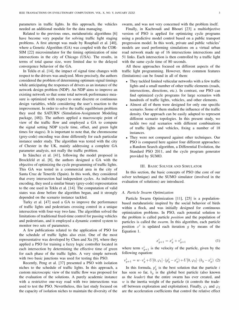
As Fig. 2 illustrates, when PSO generates a new solutionit is immediately used for updating the cycle program. Then,SUMO is started to simulate the scenario instance with streets,
IEEE TRANSACTIONS ON EVOLUTIONARY COMPUTATION, VOL. X, NO. Y, JANUARY ZZZZ 7
PSOOptimization algorithm
providing solutions SUMOTraffic simulator for
solution evaluation
SUMO InstanceInstance.add.xml
i
i-1
i+1fitness(i)
Simulation output
trace processing
Fig. 2. Optimization strategy for the cycle program configuration of trafficlights. The algorithm invokes SUMO for each solution evaluation
directions, obstacles, traffic lights, vehicles, speed, routes, etc.,under the new defined staging of cycle programs. After thesimulation, SUMO returns the global information necessaryto compute the fitness function. Each solution evaluationrequires only one simulation procedure since vehicle routes inSUMO were generated deterministically. In fact, as suggestedin [34], stochastic traffic simulators obtain similar results todeterministic ones, the latter allowing huge computing savings.
In addition, we must note that each new cycle programis statically loaded for each simulation procedure. Our aimhere is not to generate cycle programs dynamically during anisolated simulation as done in agent-based algorithms [27], butobtaining optimized cycle programs for a given scenario andtimetable. In fact, what real traffic light schedulers actuallydemand are constant cycle programs for specific areas andfor preestablished time periods (rush hours, nocturne periods,etc.), which led us to take this focus.
V. METHODOLOGY OF OUR STUDY
This section presents the experimental framework followedto assess the performance of our optimization solver. First,we describe the traffic light scenario instances generatedspecifically for this work. Later, the implementation detailsand parameter settings are presented.
A. Instances
As we are interested in developing an optimization solvercapable of dealing with close-to-reality and generic urbanareas, we have generated two scenarios by extracting actualinformation from real digital maps. These two scenarios coversimilar areas of approximately 0.42km2, and are physicallylocated in the cities of Bahıa Blanca in Argentina, and Malagain Spain. The information used concerns: traffic rules, trafficelement locations, buildings, road directions, streets, inter-sections, etc. Moreover, we have set the number of vehiclescirculating, as well as their speeds by following current speci-fications available in the Mobility Delegation of the City Hallof Malaga (http://movilidad.malaga.eu/). This information wascollected from sensorized points in certain streets obtaining ameasure of traffic density in several time intervals. In the caseof Bahıa Blanca we could not obtain such an information, andhence we considered the same number of vehicles as used forthe Malaga scenario.
In Fig. 3, the selected areas of the two cities are shownwith their corresponding capture views of OpenStreetMap
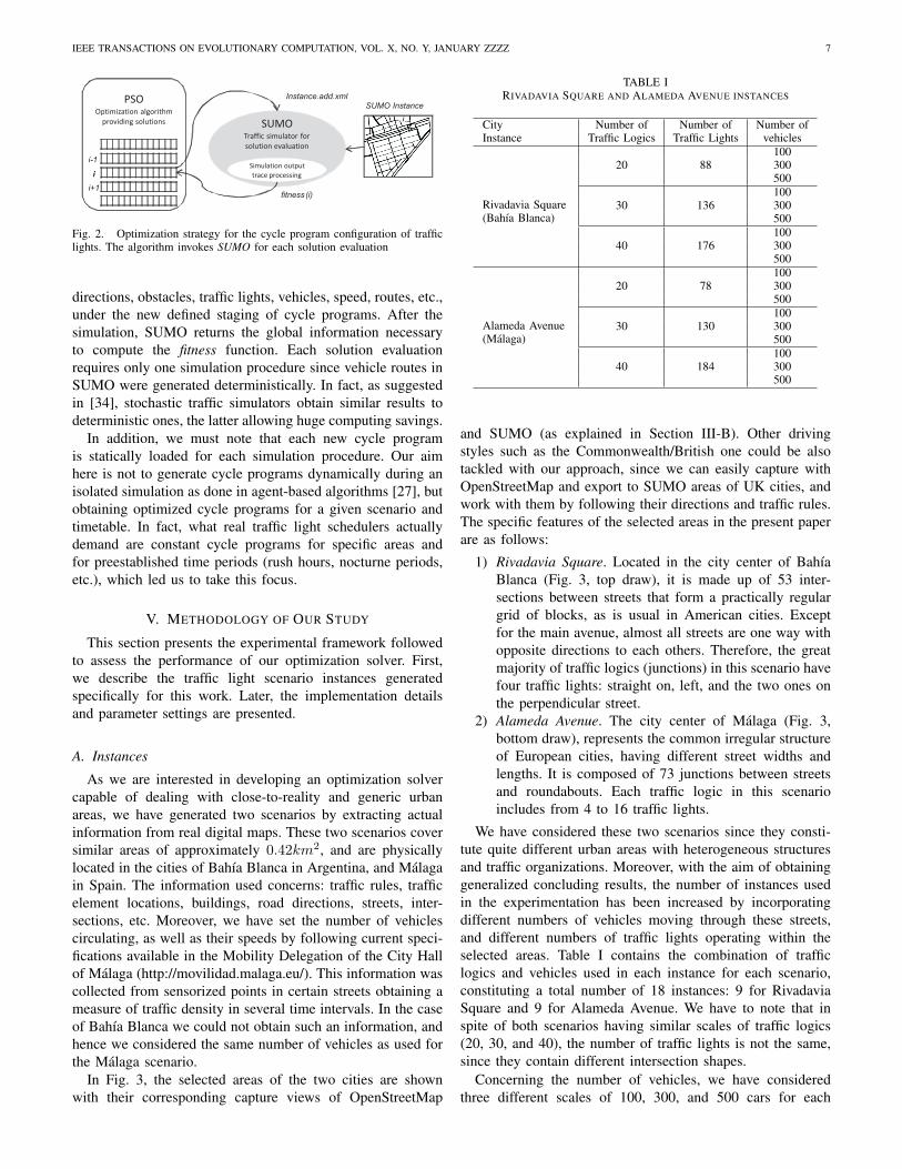
TABLE IRIVADAVIA SQUARE AND ALAMEDA AVENUE INSTANCES
City Number of Number of Number ofInstance Traffic Logics Traffic Lights vehicles
Rivadavia Square
100
(Bahıa Blanca)
20 88 300500100
30 136 300500100
40 176 300500
Alameda Avenue
100
(Malaga)
20 78 300500100
30 130 300500100
40 184 300500
and SUMO (as explained in Section III-B). Other drivingstyles such as the Commonwealth/British one could be alsotackled with our approach, since we can easily capture withOpenStreetMap and export to SUMO areas of UK cities, andwork with them by following their directions and traffic rules.The specific features of the selected areas in the present paperare as follows:
1) Rivadavia Square. Located in the city center of BahıaBlanca (Fig. 3, top draw), it is made up of 53 inter-sections between streets that form a practically regulargrid of blocks, as is usual in American cities. Exceptfor the main avenue, almost all streets are one way withopposite directions to each others. Therefore, the greatmajority of traffic logics (junctions) in this scenario havefour traffic lights: straight on, left, and the two ones onthe perpendicular street.
2) Alameda Avenue. The city center of Malaga (Fig. 3,bottom draw), represents the common irregular structureof European cities, having different street widths andlengths. It is composed of 73 junctions between streetsand roundabouts. Each traffic logic in this scenarioincludes from 4 to 16 traffic lights.
We have considered these two scenarios since they consti-tute quite different urban areas with heterogeneous structuresand traffic organizations. Moreover, with the aim of obtaininggeneralized concluding results, the number of instances usedin the experimentation has been increased by incorporatingdifferent numbers of vehicles moving through these streets,and different numbers of traffic lights operating within theselected areas. Table I contains the combination of trafficlogics and vehicles used in each instance for each scenario,constituting a total number of 18 instances: 9 for RivadaviaSquare and 9 for Alameda Avenue. We have to note that inspite of both scenarios having similar scales of traffic logics(20, 30, and 40), the number of traffic lights is not the same,since they contain different intersection shapes.
Concerning the number of vehicles, we have consideredthree different scales of 100, 300, and 500 cars for each

IEEE TRANSACTIONS ON EVOLUTIONARY COMPUTATION, VOL. X, NO. Y, JANUARY ZZZZ 8
Rivadavia Square
Bahía Blanca
Argentina
Alameda Avenue
Málaga
Spain
Google Map view OpenStreetMap view SUMO capture view
Fig. 3. Process of creation of real-world instances for study. Rivadavia Square (38◦43’03”S 62◦15’56”O) and Alameda Avenue (36◦43’60”N 4◦25’87”O)instance views. After selecting our area of interest (Google map view), it is interpreted by means of the OpenStreetMap tool, and then exported to SUMO inXML format
instance (as shown in Table I) circulating throughout thesimulation time. Each one of the vehicles performs its ownroute from origin to destination circulating with a maximumspeed of 50 km/h (typical in urban areas). The routes werepreviously generated by following random paths and coveringas much as possible all network entries. Starting times ofvehicles were also uniform randomly specified throughout thewhole simulation. This means that, at the same time, onlya subset of the whole set of vehicles is circulating throughthe network. The simulation time was fixed to 500 seconds(iterations of microsimulation) for each instance. This timewas determined as a maximum time for a car to complete itsroute, even if it must stop at all the traffic lights it comesacross. When a vehicle leaves the scenario network, it willnot appear again.
B. Experimental Setup
We have used the implementation of the PSO algorithmprovided by MALLBA [3], a C++ based framework of meta-heuristic algorithms for solving optimization problems. Thesimulation phase is carried out by executing (in the evaluationof particles) the traffic simulator SUMO release 0.12.0 forLinux. The experiments were performed in computers at thelaboratories of the Department of Computer Science of theUniversity of Malaga (Spain). Most of them are equipped withmodern dual core processors, 1GB RAM, and Linux DebianO.S. They operate under a Condor [45] middleware platformthat acts as a distributed task scheduler (each task dealing withone independent run of PSO).
TABLE IISIMULATION AND PSO PARAMETERS
Solver Phase Parameter ValueSimulation Time (steps) 500 sec.Simulation Area 0.45 km2
Simulation Details Number of Vehicles 100/300/500Vehicle Speed 0-50 km/hN. of Traffic Logics 20/30/40Max. N. of Evaluations 30,000Swarm Size 100
Particle Size (N. Traffic Lights) 88/136/17678/130/184
PSO Parameters Local Coefficient (φ1) 2.05Social Coefficient (φ2) 2.05Maximum Inertia (wmax) 0.5Minimum Inertia (wmin) 0.1Velocity Truncation Factor (λ) 0.5
For each scenario instance we have carried out 30 inde-pendent runs of our PSO. The swarm (population) size wasset to 100 particles performing 300 iteration steps, henceresulting in 30,000 solution evaluations (SUMO simulations)per run and instance. The choice of these two parameters(swarm size and maximum iteration steps) corresponds toprevious tuning experiments as described in Section VI-A. Theparticle size directly depends on the number of traffic lights ofeach instance (shown in Table I). The remaining parametersare summarized in Table II. These parameters were set afterpreliminary executions of PSO with the smallest instancesof Rivadavia Square and Alameda Avenue (with 20 trafficlogics and 100 vehicles). Specific parameters of PSO wereselected as recommended in the studies about the convergencebehavior of this algorithm in [10] and [12]. According to

IEEE TRANSACTIONS ON EVOLUTIONARY COMPUTATION, VOL. X, NO. Y, JANUARY ZZZZ 9
Algorithm 2 Pseudocode of RANDOM1: initializeSolution(x)2: i← 03: while i < Max Number of Evaluations do4: generate(xi) //new solution5: if f(x) ≥ f(xi) then6: x← xi
7: end if8: i← i+ 19: end while
these, acceleration coefficients φ1 and φ2 were set to 2.05and inertia weight decreases linearly along with the incrementof the iteration steps from 0.5 to 0.1.
Additionally, we have implemented three algorithms also inthe scope of the MALLBA [3] library, with the aim of estab-lishing comparisons against our PSO. These three algorithmsare a Random Search (RANDOM), a Differential Evolution(DE) [38], and the Standard PSO 2011 (SPSO2011) [13].Thus, performing the same experimentation procedure, weexpect to obtain some insights into the power of our proposal(how much intelligent it is) regarding a technique without anyheuristic information in its operation (RANDOM), and with re-gards to two other difference-vector based metaheuristics: DE,and SPSO2011. In the case of SPSO2011, it is the last PSOproposal in [13] and uses a different quantisation/discretizationmethod to our PSO. The maximum number of evaluations wasset to 30, 000, as for PSO.
1) Random Search: The pseudocode of the Random Searchalgorithm is shown in Algorithm 2. It basically performs bykeeping just the best solution found so far in the optimizationprocedure.
2) Differential Evolution: In DE, the task of generating newindividuals is performed by differential operators such as thedifferential mutation and crossover. A mutant individual wi
g+1
is generated by the following equation (7):
wig+1 = vr1g + F · (vr2g − vr3g ) (7)
where r1, r2, r3 ∈ {1, 2, . . . , i− 1, i+ 1, . . . , N} are randomintegers mutually different, and also different from the indexi. The mutation constant F > 0 stands for the amplificationof the difference between the individuals vr2g and vr3g , and itavoids the stagnation of the search process.
In order to increase even more the diversity in the popula-tion, each mutated individual undergoes a crossover operationwith the target individual vig, by means of which a trialindividual ui
g+1 is generated. A randomly chosen positionis taken from the mutant individual to prevent that the trialindividual replicating the target individual.
uig+1(j) =
{wi
g+1(j) if r(j) ≤ Cr or j = jr,
vig(j) otherwise.(8)
As shown in Equation 8, the crossover operator randomlychooses a uniformly distributed integer value jr and a randomreal number r ∈ (0, 1), also uniformly distributed for eachcomponent j of the trial individual ui
g+1. Then, the crossover
Algorithm 3 Pseudocode of DE1: initializePopulation()2: while g < maxIterations do3: for each individual vig do4: choose mutually different(r1, r2, r3)5: wi
g+1 = mutation(vr1g , vr2g , vr3g , F ) //Eq. 76: ui
g+1 = crossover(vig, wig+1, cp) //Eq. 8
7: evaluate(uig+1)
8: vig+1 = selection(vig, uig+1) //Eq. 9
9: end for10: end while
probability Cr, and r are compared just like j and jr. If r islower or equal than Cr (or j is equal to jr) then we selectthe jth element of the mutant individual to be allocated in thejth element of the trial individual ui
g+1. Otherwise, the jth
element of the target individual vig becomes the jth elementof the trial individual. For this work, F and Cr have been setto 0.5 and 0.9, respectively, as initially recommended in [38].
Finally, a selection operator decides on the acceptance ofthe trial individual for the next generation if and only if ityields a reduction (assuming minimization) in the value of thefitness function f(), as shown by the following Equation (9):
vig+1 =
{uig+1 if f(ui
g+1) ≤ f(vig),
vig otherwise.(9)
Algorithm 3 shows the pseudocode of DE. After initializingthe population, the individuals evolve during a number ofiterations (maxIterations). Each individual is then mutated(Line 5) and recombined (Line 6). The new individual isselected (or not) following the operation of Equation 9 (Lines 7and 8).
For the sake of a fair comparison, we also adapted the DEfor dealing with integer values in the solution codification,that is, using the same mechanism of ceiling/flooring (⌈.⌉/⌊.⌋)functions as done in the velocity vector calculation of PSO(Equation 5).
wig+1(j) =
{⌊wi
g+ 12
(j)⌋ if U(0, 1)i(j) ≤ λ
⌈wig+ 1
2
(j)⌉ otherwise(10)
In the case of DE, the truncation method is applied to themutant vector wi
g+1, as specified in Equation 10, also withλ = 0.5.
3) Standard PSO 2011: We have selected the StandardPSO 2011 (to compare with our proposal) from all theexisting versions of PSO in the literature, since it includesa series of new advances proposed by prominent researchesin this area [13]. Some of these interesting advances consistof: rotation invariance method, new particles generation inhypersphere, Gaussian random number generator, and MidTread quantisation/discretization method.
The main feature of the Standard PSO 2011 consists inthe velocity vector (vig+1) calculation which is given byEquation 11.
vig+1 = w · vig +Grig − xig +HS(Gr, ∥ Gr − xg ∥) (11)
IEEE TRANSACTIONS ON EVOLUTIONARY COMPUTATION, VOL. X, NO. Y, JANUARY ZZZZ 10
Algorithm 4 Pseudocode of Standard PSO 20111: initializeSwarm()2: while g < maxIterations do3: for each particle xi
g do4: bng =bestNeighbourSelection(xi
g, n)5: vig+1=updateVelocity(w, vig, xg, φ1, pg, φ2, b
ng )
6: xig+1=Q(updatePosition(xi
g, vig+1))
7: evaluate(xig+1)
8: pig+1=update(pig)9: end for
10: end while
with
Grig =xig + p′ig + l′ig
3(12)
p′ig = xig + c · (pig − xi
g) (13)
l′ig = xig + c · (lig − xi
g) (14)
In these formulas, pig is the best solution that the particlei has seen so far, lig is the best particle of a neighborhoodof k other particles (also known as the social best) randomly(uniform) selected from the swarm, and w is the inertia weightof the particle (it controls the trade-off between explorationand exploitation). The acceleration coefficient c > 1 is anormal (Gaussian) random value with µ = 1/2 and ρ = 1/12.This coefficient is sampled anew for each component of thevelocity vector. Finally, HS [13] is a distinctive element of theStandard PSO 2011 with regards to the previous ones. HS isbasically a random number generator within a Hyperspherespace, with Gr as center of gravity. That is, Gr is calculatedas the equidistant point to p′g, l′g , and xg .
Since the optimal cycle programming requires solutions en-coded with a vector of integers (representing phase durations),we have used the quantisation method provided in the standardspecification of PSO 2011 [13]. This quantisation is appliedto each new generated particle (in Equation 1), and transformsthe continuous values of particles to discrete ones. It consistsof a Mid-Thread uniform quantiser method as specified inEquation 15. The quantum step is set here to ∆ = 1.
Q(x) = ∆ · ⌊x/∆+ 0.5⌋ (15)
Algorithm 4 describes the pseudo-code of the Standard PSO2011. The algorithm starts by initializing the swarm (Line 1).The corresponding elements of each particle (solutions) areinitialized with random values representing the phase dura-tions. These values are within the time interval [5, 60] ∈ Z+,and constitute the range of possible time spans (in seconds).Then, for a maximum number of iterations, each particlemoves through the search space updating its velocity andposition (Lines 4, 5, and 6), it is then evaluated (Line 7), andits personal best position pi is also updated (Line 8). Finally,the best particle found so far is returned.
1
1.5
2
2.5
3
3.5
4
4.5
5
5.5
6
6.5
0 50 100 150 200 250 300 350 400 450 500
Max Iter=300Max Iter=100
Be
st F
itn
ess
Number of Iterations
Alameda with 30 Traffic Logics - 30 Vehicles
Swarm Size= 50 Max Iter=100Swarm Size=100 Max Iter=100Swarm Size=200 Max Iter=100Swarm Size= 50 Max Iter=300Swarm Size=100 Max Iter=300Swarm Size=200 Max Iter=300Swarm Size= 50 Max Iter=500Swarm Size=100 Max Iter=500Swarm Size=200 Max Iter=500
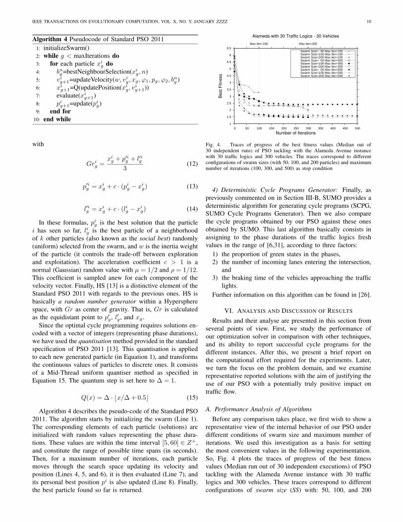
Fig. 4. Traces of progress of the best fitness values (Median out of30 independent runs) of PSO tackling with the Alameda Avenue instancewith 30 traffic logics and 300 vehicles. The traces correspond to differentconfigurations of swarm sizes (with 50, 100, and 200 particles) and maximumnumber of iterations (100, 300, and 500) as stop condition
4) Deterministic Cycle Programs Generator: Finally, aspreviously commented on in Section III-B, SUMO provides adeterministic algorithm for generating cycle programs (SCPG,SUMO Cycle Programs Generator). Then we also comparethe cycle programs obtained by our PSO against these onesobtained by SUMO. This last algorithm basically consists inassigning to the phase durations of the traffic logics freshvalues in the range of [6,31], according to three factors:
1) the proportion of green states in the phases,2) the number of incoming lanes entering the intersection,
and3) the braking time of the vehicles approaching the traffic
lights.Further information on this algorithm can be found in [26].
VI. ANALYSIS AND DISCUSSION OF RESULTS
Results and their analyse are presented in this section fromseveral points of view. First, we study the performance ofour optimization solver in comparison with other techniques,and its ability to report successful cycle programs for thedifferent instances. After this, we present a brief report onthe computational effort required for the experiments. Later,we turn the focus on the problem domain, and we examinerepresentative reported solutions with the aim of justifying theuse of our PSO with a potentially truly positive impact ontraffic flow.
A. Performance Analysis of Algorithms
Before any comparison takes place, we first wish to show arepresentative view of the internal behavior of our PSO underdifferent conditions of swarm size and maximum number ofiterations. We used this investigation as a basis for settingthe most convenient values in the following experimentation.So, Fig. 4 plots the traces of progress of the best fitnessvalues (Median run out of 30 independent executions) of PSOtackling with the Alameda Avenue instance with 30 trafficlogics and 300 vehicles. These traces correspond to differentconfigurations of swarm size (SS) with: 50, 100, and 200
IEEE TRANSACTIONS ON EVOLUTIONARY COMPUTATION, VOL. X, NO. Y, JANUARY ZZZZ 11
0 50 100 150 200 250 300
1.0
1.5
2.0
2.5
40 Traffic Logics − 500 Vehicles
Number of Iterations
Bes
t Fitn
ess
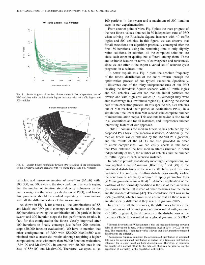
Fig. 5. Trace progress of the best fitness values in 30 independent runs ofPSO tackling with the Rivadavia Square instance with 40 traffic logics and500 vehicles
Fitness
12
3
4
5
6
7
Num
ber of
Iter
atio
ns
50
100
150
200
250
300
Absolu
teF
requency 0
20
40
60
80
100
Fitness Histogram Evolution
Fig. 6. Swarm fitness histogram through 300 iterations in the optimizationof the Rivadavia Square scenario with 40 traffic logics and 500 vehicles
particles, and maximum number of iterations (MaxIt) with:100, 300, and 500 steps to the stop condition. It is worth sayingthat the number of iteration steps directly influences on theinertia weigh (in the velocity calculation of PSO), and hence,this parameter should be studied separately in combinationwith all the different values of the swarm size.
As shown in Fig. 4, for almost all the combinations (of SSand MaxIt) our PSO got to converge on the interval of 100 and300 iterations, showing the combination of 100 particles in theswarm and 300 iteration steps the best performance results. Infact, for this configuration the fitness clearly improved after100 iterations to finally converge just before 200 iterationsteps (20,000 function evaluations). We have to mention thatother configurations of PSO with SS=200 MaxIt=500 alsoobtained such a successful results although requiring a highercomputational cost with more than 50,000 function evaluations(SS=100 and MaxIt=500), in contrast with 30,000 ones in thecase of SS=100 and MaxIt=300. Therefore, we opted to set
100 particles in the swarm and a maximum of 300 iterationsteps in our experimentation.
From another point of view, Fig. 5 plots the trace progress ofthe best fitness values obtained in 30 independent runs of PSOwhen solving the Rivadavia Square instance with 40 trafficlogics and 500 vehicles. In this figure, we can observe thatfor all executions our algorithm practically converged after thefirst 150 iterations, using the remaining time to only slightlyrefine solutions. In addition, all the computed solutions areclose each other in quality, but different among them. Theseare desirable features in terms of convergence and robustness,since we can offer to the expert a varied set of accurate cycleprograms in a reduced time.
To better explain this, Fig. 6 plots the absolute frequencyof the fitness distribution of the entire swarm through theoptimization process of one typical execution. Specifically,it illustrates one of the thirty independent runs of our PSOtackling the Rivadavia Square scenario with 40 traffic logicsand 500 vehicles. We can see that the initial particles arediverse and with high cost values (≃ 7), although they wereable to converge in a low fitness region (≤ 1) during the secondhalf of the execution process. In this specific run, 475 vehiclesout of 500 reached their particular destinations (95%) in asimulation time lower than 500 seconds (the complete numberof microsimulation steps). This accurate behavior is also foundin all executions and for all instances, and it represents anotherinteresting feature of our approach.
Table III contains the median fitness values obtained by theproposed PSO for all the scenario instances. Additionally, themedian fitness values obtained by the RANDOM algorithm,and the results of the SCPG are also provided in orderto allow comparisons. We can easily check in this tablethat PSO obtained the best median fitness (marked in bold)independently of both, the number of vehicles and the numberof traffic logics in each scenario instance.
In order to provide statistically meaningful comparisons, wehave applied a Signed Ranked (Wilcoxon) 2 test [49] to thenumerical distributions of the results. We have used this non-parametric test since the resulting distributions usually violatethe condition of normality required to apply parametric tests(Z Kolmogorov-Smirnov = 0.04) 3 . Another implication of theviolation of the normality condition is the use of median values(as shown in Table III) instead of other measures like the meanand the standard deviation [42]. The confidence level was set to95% (α=0.05), which allows us to ensure that all these resultsare statistically different if they result in p-value<0.05.
In effect, for all the instances, the differences between thedistributions out of 30 independent runs resulted with p-values<< 0.05. In general, the differences in the distributions of themedians (Table III) resulted in a global p-value of 5.73E-7
2The null hypothesis in Wilcoxon test is that the median difference betweenpairs of observations is zero, with a confidence level of 95% (α=0.05) in ourcase. This means that, if resulted p-value is lower than 0.05, then the compareddistributions are different.
3Kolmogorov-Smirnov compares the accumulated distribution of observeddata with the accumulated distribution expected for a Gaussian distribution,obtaining the p-value based on both discrepancies. Therefore, it measuresthe quality of a normal fitting to the data and then can be used to test thehypothesis of normality in the population distribution.
IEEE TRANSACTIONS ON EVOLUTIONARY COMPUTATION, VOL. X, NO. Y, JANUARY ZZZZ 12
TABLE IIIMEDIAN FITNESS VALUES OBTAINED BY PSO FOR ALL THE SCENARIO INSTANCES. MEDIAN FITNESS OBTAINED BY RANDOM AND BY SCPG
ALGORITHMS ARE ALSO PROVIDED. NTL IS THE NUMBER OF TRAFFIC LOGICS
Instance NTLNumber of Vehicles
100 300 500PSO RANDOM SCPG PSO RANDOM SCPG PSO RANDOM SCPG
20 1.64E+00 2.91E+00 2.38E+00 8.40E-01 1.45E+00 9.24E-01 7.93E-01 1.51E+00 9.56E-01Rivadavia Square 30 1.80E+00 3.11E+00 2.45E+00 9.09E-01 1.65E+00 9.57E-01 8.79E-01 1.72E+00 9.89E-01
40 1.79E+00 3.08E+00 2.49E+00 9.11E-01 1.75E+00 9.76E-01 8.96E-01 1.74E+00 9.93E-0120 9.47E-01 1.68E+00 1.49E+00 8.44E-01 1.62E+00 1.29E+00 4.10E+00 7.87E+00 2.35E+01
Alameda Avenue 30 1.56E+00 3.55E+00 5.12E+00 1.74E+00 4.52E+00 6.00E+00 7.67E+00 1.33E+01 3.31E+0140 1.88E+00 3.98E+00 5.38E+00 2.87E+00 7.33E+00 1.83E+01 9.39E+00 1.64E+01 1.47E+01
100 300 500
0.5
1.0
1.5
2.0
2.5
3.0
3.5
20 Traffic Logics
Number of Vehicles
Fitn
ess
100 300 500
0.5
1.0
1.5
2.0
2.5
3.0
3.5
100 300 500
0.5
1.0
1.5
2.0
2.5
3.0
3.5
20 Traffic Logics
Number of Vehicles
Fitn
ess
PSO
PSOPSO
Rando
m
Rando
mRan
dom
100 300 500
0.5
1.0
1.5
2.0
2.5
3.0
3.5
4.0
30 Traffic Logics
Number of Vehicles
Fitn
ess
100 300 500
0.5
1.0
1.5
2.0
2.5
3.0
3.5
4.0
100 300 500
0.5
1.0
1.5
2.0
2.5
3.0
3.5
4.0
30 Traffic Logics
Number of Vehicles
Fitn
ess
PSO
PSO
PSO
Rando
m
Rando
m
Rando
m
100 300 500
0.5
1.0
1.5
2.0
2.5
3.0
3.5
40 Traffic Logics
Number of Vehicles
Fitn
ess
100 300 500
0.5
1.0
1.5
2.0
2.5
3.0
3.5
100 300 500
0.5
1.0
1.5
2.0
2.5
3.0
3.5
40 Traffic Logics
Number of Vehicles
Fitn
ess
PSO
PSO PSO
Rando
m
Rando
m
Rando
m
100 300 500
510
1520
20 Traffic Logics
Number of Vehicles
Fitn
ess
100 300 500
510
1520
100 300 500
510
1520
20 Traffic Logics
Number of Vehicles
Fitn
ess
PSOPSO
PSO
Rando
m
Rando
m
Rando
m
100 300 500
05
1015
2025
3035
30 Traffic Logics
Number of Vehicles
Fitn
ess
100 300 500
05
1015
2025
3035
100 300 500
05
1015
2025
3035
30 Traffic Logics
Number of Vehicles
Fitn
ess
PSO PSO
PSO
Rando
mRan
dom
Rando
m
100 300 500
510
1520
40 Traffic Logics
Number of Vehicles
Fitn
ess
100 300 500
510
1520
100 300 500
510
1520
40 Traffic Logics
Number of Vehicles
Fitn
ess
PSO PSO
PSO
Rando
m
Rando
m
Rando
m
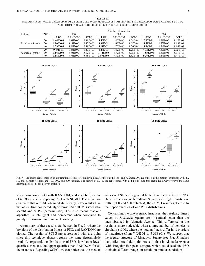
Fig. 7. Boxplots representation of distributions results of Rivadavia Square (three at the top) and Alameda Avenue (three at the bottom) instances with 20,30, and 40 traffic logics, and 100, 300, and 500 vehicles. The results of SCPG are represented with a � point since this technique always returns the samedeterministic result for a given instance
when comparing PSO with RANDOM, and a global p-valueof 6.33E-5 when comparing PSO with SUMO. Therefore, wecan claim that our PSO obtained statistically better results thanthe other two compared algorithms: RANDOM (stochasticsearch) and SCPG (deterministic). This also means that ouralgorithm is intelligent and competent when compared togreedy information and human knowledge.
A summary of these results can be seen in Fig. 7, where theboxplots of the distribution fitness of PSO, and RANDOM areplotted. The results of SCPG are represented with a � pointsince this technique always returns the same deterministicresult. As expected, the distributions of PSO show better lowerquartiles, medians, and upper quartiles than RANDOM for allthe instances. Regarding SCPG, we can notice that the median
values of PSO are in general better than the results of SCPG.Only in the case of Rivadavia Square with high densities oftraffic (300 and 500 vehicles), the SUMO results get close tothe upper quartiles of our PSO distributions.
Concerning the two scenario instances, the resulting fitnessvalues in Rivadavia Square are in general better than theones obtained in Alameda Avenue. This difference in theresults is more noticeable when a large number of vehicles iscirculating (500), where the median fitness differ in two ordersof magnitude (from 7.93E-01 to 3.31E+01). We suspect thatthe regular structure of Rivadavia Square (see Fig. 3) makesthe traffic more fluid in this scenario than in Alameda Avenua(with irregular European design), which could lead the PSOto obtain different ranges of results in similar conditions.

IEEE TRANSACTIONS ON EVOLUTIONARY COMPUTATION, VOL. X, NO. Y, JANUARY ZZZZ 13
TABLE IVMEDIAN FITNESS VALUES OBTAINED BY OUR PSO, DE, AND STANDARD PSO 2011 FOR ALL THE SCENARIO INSTANCES. NTL IS THE NUMBER OF
TRAFFIC LOGICS
Instance NTLNumber of Vehicles
100 300 500PSO DE SPSO2011 PSO DE SPSO2011 PSO DE SPSO2011
20 1.64E+00 2.18E+00 1.87E+00 8.40E-01 9.94E-01 9.82E-01 7.93E-01 9.80E-01 1.22E+00Rivadavia Square 30 1.80E+00 2.25E+00 2.33E+00 9.09E-01 1.11E+00 1.28E+00 8.79E-01 1.02E+00 1.44E+00
40 1.79E+00 2.23E+00 2.50E+00 9.11E-01 1.13E+00 1.25E+00 8.96E-01 1.10E+00 1.40E+0020 9.47E-01 1.22E+00 1.11E+00 8.44E-01 1.07E+00 9.12E-01 4.10E+00 4.98E+00 4.71E+00
Alameda Avenue 30 1.56E+00 2.19E+00 2.49E+00 1.74E+00 2.54E+00 3.47E+00 7.67E+00 8.57E+00 1.11E+0140 1.88E+00 2.54E+00 3.21E+00 2.87E+00 4.06E+00 5.32E+00 9.39E+00 1.17E+01 1.30E+01
B. Comparison with Other Metaheuristic Algorithm:Differential Evolution and Standard PSO 2011
For a further comparison, we have studied the performanceof two other metaheuristic algorithms for the same experi-mental procedure as with our proposal. A first comparisonconcerns a Differential Evolution algorithm (as described inSection V-B), by means of which we expect to better justifythe use of PSO on the cycle program of traffic lights. Secondly,we compare our PSO against the Standard PSO 2011 whichperforms a different velocity calculation and discretizationmethod.
The median fitness values (out of 30 independent runs)resulted in the experimentation of DE and SPSO2011 areincluded in Table IV together with the ones of our PSO forthe two scenario instances, Rivadavia Square and AlamedaAvenue. Again, we confirm that the PSO obtained the bestmedian fitness for all the combinations of number of vehiclesand number of traffic logics in each scenario instance. Ingeneral, using a Wilcoxon Signed Rank test with α=0.05,the differences in the distributions of the medians (Table IV)resulted in a global p-value of 1.94E-4 when comparing PSOwith DE, and a global p-value of 1.96E-4 when comparingPSO with SPSO2011. In the first case, the different learningprocedures that our PSO and DE perform is the main fac-tor that influences the statistical differences in results, sincethese two algorithms used the same discretization method.In the second case, the different velocity calculation methodsinfluence the algorithms’ performances of our PSO and SPSO2011, indicating that our proposal is better than the lastStandard PSO for the tackled problem.
As a further comparison, SPSO2011 showed better fitnessvalues than DE, resulting a global p-value of 1.47E-2. If wetake into account that DE uses a similar discretization methodas to our PSO, the last results lead us to suspect that thedifferent discretization of vectors marginally influences on theglobal algorithm’s performance.
Therefore, in the scope of the experimental frameworkadopted in this approach, we can claim that our PSO alsoobtained statistically better results than the other metaheuristicapproaches (DE and SPSO2011) used to solve the optimalcycle program of traffic lights.
C. Scalability Analysis
To study the scalability of our proposal, we now focus onthe influence of the two main factors defining the complexity
5,00E-01
1,00E+01
2,00E+02
20 30 40
Number of Traffic Logics - Alameda Avenue
100 Vehicles
300 Vehicles
500 Vehicles
Number of Traffic
Lights
Fig. 8. Increment of the median fitness with regards to the number of trafficlights for the Alameda Avenue scenario. The values are in logarithmic scale
of the instances: the number of traffic logics (20, 30, and 40),and the number of vehicles circulating (100, 300, and 500).
The first observation concerns the number of traffic logics(and hence, the number of traffic lights), since it determinesthe dimensionality of the problem. In Fig. 8, we can observethat the mean fitness values increase with the number of trafficlogics, as expected. Although, this increment is moderate withregards to the number of traffic lights (dotted lines).
A second interesting observation can be obtained fromFig. 7, where the distribution of results concerning the numberof vehicles are completely different for both scenarios. Thus,in Alameda Avenue (three boxplots in the top) the distributionof results gets worse with an increasing number of vehicles.This seems logical since a high number of cars increases thepossibility of generating traffic jams. In addition, we musttake into account that the number of vehicles that arrive totheir destinations directly influences the fitness function. To thecontrary, in Rivadavia Square (three boxplots in the bottom)the distributions of results improve as the number of vehiclesincreases. In this case, we suspect that the particular shapeof this scenario, with parallel streets and thus organized flow,could influence in the number of vehicles that quickly reachtheir destinations and leave the scenario, hence introducinggreat benefits to the fitness calculation.
D. Computational Effort
Table V contains the mean times (and standard deviations)in seconds required by our PSO to compute all the experi-ments. We must state that these times are averaged, since they

IEEE TRANSACTIONS ON EVOLUTIONARY COMPUTATION, VOL. X, NO. Y, JANUARY ZZZZ 14
TABLE VMEAN TIME AND STANDARD DEVIATION IN SECONDS OF OUR PSO TO COMPUTE ALL THE EXPERIMENTS
Instance Number of Traffic Logics Number of Vehicles100 300 500
20 4.14E+02±6.74E+01 5.94E+02±6.83E+01 7.25E+02±6.53E+01Rivadavia Square 30 4.09E+02±6.11E+01 5.04E+02±5.54E+01 7.44E+02±6.51E+01
40 3.56E+02±5.42E+01 4.43E+02±4.60E+01 6.66E+02±5.66E+0120 4.30E+02±4.55E+01 1.20E+03±7.58E+01 1.59E+03±9.50E+01
Alameda Avenue 30 5.46E+02±5.48E+01 1.14E+03±7.43E+01 1.51E+03±8.59E+0140 5.12E+02±5.12E+01 1.23E+03±8.03E+01 1.48E+03±8.51E+01
were calculated in the scope of a Condor [45] middleware witha pool of machines with different specifications.
The lowest execution time (3.56E+02 seconds) was requiredfor solving the Rivadavia Square scenario with 40 traffic logicsand 100 vehicles. The highest time (1.59E+03 seconds) wasused in the resolution of Alameda Avenue scenario with 20traffic lights and 500 vehicles. All these times are in a rangefrom 6.33 to 26.5 minutes, which is completely aceptable tothe human experts in civil engineering designing and takingdecisions on the traffic network.
We stress that the computing time increases with the numberof vehicles (common sense), although it decreases with thenumber of traffic lights (counterintuitive). This fact can be dueto the optimized cycle programs that control a great number oftraffic lights. These optimized traffic lights enhance the trafficflow leading the cars to get their destinations quickly, hencereducing the computing load of simulation.
E. Analysis of Solutions
Finally, in this section we focus on the cycle programsobtained as solutions by our PSO, and the possible profitsthey can offer to the actual users in this field. Then weshow the broad impact of using our optimization technique,able to compute realistic and comprehensive traffic light cycleprograms.
In this context, for each iteration step of the PSO and foreach particle in the swarm, we have saved the informationobtained from each simulation (solution evaluation) aboutboth, the number of vehicles that reached their destinationsand the average duration of their journeys. This way, we candistinguish the progressive improvement in the traffic flowobtained from the initial solutions to the final ones, throughout the complete optimization procedure.
A representative example can be observed in the opti-mization process of the Alameda Avenue scenario with 30traffic logics (130 traffic lights in the cycle program) and 300vehicles. First, in Fig. 9 we can see the trace of the numberof vehicles that did reach their destinations (upper continuousline) versus the number of vehicles that did not reach theirdestinations (lower dotted line) for each iteration step in arun of PSO. The overlapped curves show the mean numberof vehicles (out of 30 independent runs) that did arrive anddid not arrive at their destinations. In contrast, this figurealso shows the results (in dotted straight lines) of the SCPG(SUMO algorithm) for this same instance.
We can easily see in Fig. 9 how the amount of vehiclesthat did arrive (did not arrive) to their destinations increases
0 50 100 150 200 250 300
050
100
150
200
250
300
30 Traffic Logics - 300 Vehicles
Number of Iterations
Num
ber
of V
ehic
les
Vehicles that
did arrive
did not arrive
(SCPG) did arrive
(SCPG) did not arrive
Fig. 9. Number of Vehicles that did reach their destinations (continuouslines) versus vehicles that did not reach their destinations (dotted lines) in thestudied time frame. Overlapped curves show the mean number of vehicles (outof 30 independent runs) that did arrive and did not arrive at their destinations.SCPG results are also shown with dotted straight lines
(decreases) as the algorithm gets the stop condition of 300iterations. In fact, at the initial steps of the optimization pro-cess, the number of vehicles that reached their destinations waslower than the ones resulting in the cycle program generatedby SCPG. However, in the final steps of the PSO procedure,the solutions obtained show a high quality in terms of thetraffic flow, since 295 vehicles of the initial 300 (98.33%)finalized their trips successfully. Moreover, a mean numberof 255 vehicles completed their trips in the final solutions ofPSO (average of 30 runs). This contrast to the 160 vehiclesthat reached their destinations in the SUMO cycle program.The improvement obtained by our PSO over SCPG is 31.66%.
Another interesting behavior that can be observed in Fig. 9is the alternating peaks and valleys that appear in the curves ofthe single run of PSO. These peaks represent solutions withan accurate fitness but with a low number of cars reachingtheir destinations. This can be due to the fact that, the fitnessfunction (Equation 3) promotes cycle programs with largedurations of phases in which the proportion of traffic lightsin green is higher than in red. For certain intersections withseveral secondary streets and only one big avenue, the trafficlights controlling this avenue could extend their states in red,thus resulting in a traffic jam that could delay the traffic inother adjacent intersections/streets. A string influence on the

IEEE TRANSACTIONS ON EVOLUTIONARY COMPUTATION, VOL. X, NO. Y, JANUARY ZZZZ 15
0 50 100 150 200 250 300
250
300
350
30 Traffic Logics - 300 Vehicles
Number of Iterations
Journ
ey T
ime
SCPG
PSO
Fig. 10. Mean trip time of vehicles calculated for each one of the simulationsperformed through a representative run of PSO. SCPG results are also shownwith a dotted straight line. Y axis represents the journey time in seconds
successful trips in the fitness function (promoting the numberof vehicles that arrive and penalizing when vehicles do notarrive) leads the PSO to avoid this kind of solutions.
From a different point of view, Fig. 10 plots the trace of theaverage journey time employed by the vehicles in the resultingsolutions of PSO through all the iterations of an examplerun. In this case, the journey time becomes shorter as thealgorithm approaches the stop condition. We must note that,in the calculation of the journey time, the vehicles that didnot arrive at their destinations took 500 seconds, the completesimulation time. For this reason, SCPG solutions showed anaverage journey time of 308.75 seconds while PSO solutionsobtained a journey length of 78 seconds, which involves animprovement of 74% with respect to the SCPG solution. Inthis specific case, 295 vehicles (of 300) completed their tripduring the simulation time with an average journey time of 78seconds to complete the urban scenario of 650 × 650 meters.In the worst case, the remaining five vehicles will completetheir trips in at most 500+78 seconds, that is, the completesimulation time plus the average journey time.
Finally, with the aim of clarifying the final implications ofusing (or not using) an optimized cycle program, Fig. 11 showsthe simulation traces of the traffic flow resulting from solutionsgenerated by both, SCPG (left) and PSO (right). The pictureswere captured at the end of the simulation time (500 seconds),and correspond to two simulation procedures of the scenarioinstance Alameda Avenue with 40 traffic logics (184 trafficlights) and 500 vehicles. As we can observe, the traffic densityof the SCPG cycle program is clearly higher than the oneof PSO, even showing the former several intersections withtraffic jams. As to the PSO cycle program, all intersectionsare unblocked at the end of the study.
VII. CONCLUSIONS
In this paper, we propose an optimization technique basedon a Particle Swarm Optimization algorithm that can find suc-cessful traffic light programs. For the evaluation of solutionswe use SUMO, a well-known microscopic traffic simulator.For this study we have tested two extensive and heterogeneousmetropolitan areas located in Bahıa Blanca, and Malaga.
Out of these two scenarios, a total number of 18 differentnumerical instances have been generated depending on theamount of vehicles circulating and the number of traffic lightsoperating. A series of analyses have been carried out fromdifferent points of view: the performance of the optimizationtechnique, the scalability, the computational effort, and thequality of solutions. From these, the following conclusionscan be extracted:
1) Our PSO solver performs successfully in the generationof optimized cycle programs for big realistic trafficscenarios. For all the instances, our proposal obtainedrobust results statistically better than the other two com-pared algorithms: the SUMO cycle programs generator(SCPG) and a Random Search algorithm (RANDOM).
2) In comparison with the Differential Evolution and Stan-dard PSO 2011 algorithms, our PSO also showed a betterperformance.
3) In the scope of the scenario instances studied here, wecan claim that our PSO scales adequately in terms of thenumber of traffic lights. Concerning a growing numberof vehicles, we have characterized how the scenariotopology can influence in the scalability power of ourproposal, showing accurate results specially with regularroute designs.
4) The complete optimization process required a computa-tional mean time in the range from 6.33 to 26.5 minutes,which is completely acceptable for use by human expertsin civil engineering. Furthermore, these values suggestthat we can still work with larger scenario instances infuture experiments.
5) The final solutions obtained by our PSO can improve thenumber of vehicles that reach their destinations and themean journey time, for all the instances. In particular,for the Alameda Avenue instance with 30 traffic logicsand 300 vehicles, the improvement obtained is around31.66% in the number of completed trips and 74% inthe journey time, regarding SCPG. All this means a realimprovement in city traffic.
For future work, we will be tackling the optimal cycleprogram with other optimization techniques, and in particularother metaheuristics. We are also interested in using othertraffic simulators and creating new larger dimension instances,as close as possible to real scenarios of a whole city.
ACKNOWLEDGMENTS
Authors acknowledge funds from the Junta de Andalu-cia (CICE), under contract P07-TIC-03044 (DIRICOM projecthttp://diricom.lcc.uma.es) and Spanish Ministry of Sci-ences and Innovation (MEC) and FEDER under contract TIN2011-28194 (Roadme project http://roadme.lcc.uma.es). JoseGarcıa-Nieto is supported by grant BES-2009-018767 from the
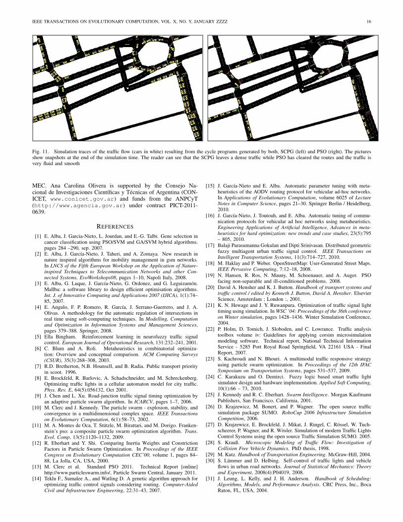
IEEE TRANSACTIONS ON EVOLUTIONARY COMPUTATION, VOL. X, NO. Y, JANUARY ZZZZ 16
Fig. 11. Simulation traces of the traffic flow (cars in white) resulting from the cycle programs generated by both, SCPG (left) and PSO (right). The picturesshow snapshots at the end of the simulation time. The reader can see that the SCPG leaves a dense traffic while PSO has cleared the routes and the traffic isvery fluid and smooth
MEC. Ana Carolina Olivera is supported by the Consejo Na-cional de Investigaciones Cientıficas y Tecnicas of Argentina (CON-ICET, www.conicet.gov.ar) and funds from the ANPCyT(http://www.agencia.gov.ar) under contract PICT-2011-0639.
REFERENCES
[1] E. Alba, J. Garcia-Nieto, L. Jourdan, and E.-G. Talbi. Gene selection incancer classification using PSO/SVM and GA/SVM hybrid algorithms.pages 284 –290, sep. 2007.
[2] E. Alba, J. Garcıa-Nieto, J. Taheri, and A. Zomaya. New research innature inspired algorithms for mobility management in gsm networks.In LNCS of the Fifth European Workshop on the Application of Nature-inspired Techniques to Telecommunication Networks and other Con-nected Systems, EvoWorkshops08, pages 1–10, Napoli Italy, 2008.
[3] E. Alba, G. Luque, J. Garcıa-Nieto, G. Ordonez, and G. Leguizamon.Mallba: a software library to design efficient optimisation algorithms.Int. J. of Innovative Computing and Applications 2007 (IJICA), 1(1):74–85, 2007.
[4] E. Angulo, F. P. Romero, R. Garcıa, J. Serrano-Guerrero, and J. A.Olivas. A methodology for the automatic regulation of intersections inreal time using soft-computing techniques. In Modelling, Computationand Optimization in Information Systems and Management Sciences,pages 379–388. Springer, 2008.
[5] Ella Bingham. Reinforcement learning in neurofuzzy traffic signalcontrol. European Journal of Operational Research, 131:232–241, 2001.
[6] C. Blum and A. Roli. Metaheuristics in combinatorial optimiza-tion: Overview and conceptual comparison. ACM Computing Surveys(CSUR), 35(3):268–308, 2003.
[7] R.D. Bretherton, N.B. Hounsell, and B. Radia. Public transport priorityin scoot. 1996.
[8] E. Brockfeld, R. Barlovic, A. Schadschneider, and M. Schreckenberg.Optimizing traffic lights in a cellular automaton model for city traffic.Phys. Rev. E, 64(5):056132, Oct 2001.
[9] J. Chen and L. Xu. Road-junction traffic signal timing optimization byan adaptive particle swarm algorithm. In ICARCV, pages 1–7, 2006.
[10] M. Clerc and J. Kennedy. The particle swarm - explosion, stability, andconvergence in a multidimensional complex space. IEEE Transactionson Evolutionary Computation, 6(1):58–73, 2002.
[11] M. A. Montes de Oca, T. Stutzle, M. Birattari, and M. Dorigo. Franken-stein’s pso: a composite particle swarm optimization algorithm. Trans.Evol. Comp, 13(5):1120–1132, 2009.
[12] R. Eberhart and Y. Shi. Comparing Inertia Weights and ConstrictionFactors in Particle Swarm Optimization. In Proceedings of the IEEECongress on Evolutionary Computation CEC’00, volume 1, pages 84–88, La Jolla, CA, USA, 2000.
[13] M. Clerc et al. Standard PSO 2011. Technical Report [online]http://www.particleswarm.info/, Particle Swarm Central, January 2011.
[14] Teklu F., Sumalee A., and Watling D. A genetic algorithm approach foroptimizing traffic control signals considering routing. Computer-AidedCivil and Infrastructure Engineering, 22:31–43, 2007.
[15] J. Garcıa-Nieto and E. Alba. Automatic parameter tuning with meta-heuristics of the AODV routing protocol for vehicular ad-hoc networks.In Applications of Evolutionary Computation, volume 6025 of LectureNotes in Computer Science, pages 21–30. Springer Berlin / Heidelberg,2010.
[16] J. Garcıa-Nieto, J. Toutouh, and E. Alba. Automatic tuning of commu-nication protocols for vehicular ad hoc networks using metaheuristics.Engineering Applications of Artificial Intelligence, Advances in meta-heuristics for hard optimization: new trends and case studies, 23(5):795– 805, 2010.
[17] Balaji Parasumanna Gokulan and Dipti Srinivasan. Distributed geometricfuzzy multiagent urban traffic signal control. IEEE Transactions onIntelligent Transportation Systems, 11(3):714–727, 2010.
[18] M. Haklay and P. Weber. OpenStreetMap: User-Generated Street Maps.IEEE Pervasive Computing, 7:12–18, 2008.
[19] N. Hansen, R. Ros, N. Mauny, M. Schoenauer, and A. Auger. PSOfacing non-separable and ill-conditioned problems. 2008.
[20] David A. Hensher and K. J. Button. Handbook of transport systems andtraffic control / edited by Kenneth J. Button, David A. Hensher. ElsevierScience, Amsterdam ; London :, 2001.
[21] K. N. Hewage and J. Y. Ruwanpura. Optimization of traffic signal lighttiming using simulation. In WSC ’04: Proceedings of the 36th conferenceon Winter simulation, pages 1428–1436. Winter Simulation Conference,2004.
[22] P. Holm, D. Tomich, J. Sloboden, and C. Lowrance. Traffic analysistoolbox volume iv: Guidelines for applying corsim microsimulationmodeling software. Technical report, National Technical InformationService - 5285 Port Royal Road Springfield, VA 22161 USA - FinalReport, 2007.
[23] S. Kachroudi and N. Bhouri. A multimodal traffic responsive strategyusing particle swarm optimization. In Proceedings of the 12th IFACSymposium on Transportation Systems, pages 531–537, 2009.
[24] C. Karakuzu and O. Demirci. Fuzzy logic based smart traffic lightsimulator design and hardware implementation. Applied Soft Computing,10(1):66 – 73, 2010.
[25] J. Kennedy and R. C. Eberhart. Swarm Intelligence. Morgan KaufmannPublishers, San Francisco, California, 2001.
[26] D. Krajzewicz, M. Bonert, and P. Wagner. The open source trafficsimulation package SUMO. RoboCup 2006 Infrastructure SimulationCompetition, 2006.
[27] D. Krajzewicz, E. Brockfeld, J. Mikat, J. Ringel, C. Rossel, W. Tuch-scheerer, P. Wagner, and R. Wosler. Simulation of modern Traffic LightsControl Systems using the open source Traffic Simulation SUMO. 2005.
[28] S. Krauß. Microscopic Modeling of Traffic Flow: Investigation ofCollision Free Vehicle Dynamics. PhD thesis, 1998.
[29] M. Kutz. Handbook of Transportation Engineering. McGraw-Hill, 2004.[30] S. Lammer and D. Helbing. Self-control of traffic lights and vehicle
flows in urban road networks. Journal of Statistical Mechanics: Theoryand Experiment, 2008(4):P04019, 2008.
[31] J. Leung, L. Kelly, and J. H. Anderson. Handbook of Scheduling:Algorithms, Models, and Performance Analysis. CRC Press, Inc., BocaRaton, FL, USA, 2004.

IEEE TRANSACTIONS ON EVOLUTIONARY COMPUTATION, VOL. X, NO. Y, JANUARY ZZZZ 17
[32] G. Lim, J. J. Kang, and Y. Hong. The optimization of traffic signal lightusing artificial intelligence. In FUZZ-IEEE, pages 1279–1282, 2001.
[33] J. McCrea and S. Moutari. A hybrid macroscopic-based model for trafficflow in road networks. European Journal of Operational Research,207(1):676–684, 2010.
[34] J. Sanchez Medina, M. Galan M., and E. Rubio Royo. Stochastic vsdeterministic traffic simulator. comparative study for its use within atraffic light cycles optimization architecture. In Jose Mira and JoseAlvarez, editors, Artificial Intelligence and Knowledge EngineeringApplications: A Bioinspired Approach, volume 3562 of Lecture Notes inComputer Science, pages 622–631. Springer Berlin / Heidelberg, 2005.
[35] T. Nagatani. Effect of speed fluctuation on green-light path in 2d trafficnetwork controlled by signals. Physica A: Statistical Mechanics and itsApplications, 389(19):4105–4115, 2010.
[36] K. E. Parsopoulos and F. M. Vrahatis. Unified particle swarm opti-mization for solving constrained engineering optimization problems. InAdvances in Natural Computation, pages 582–591. Springer, 2005.
[37] L. Peng, M.-H. Wang, J.-P. Du, and G. Luo. Isolation niches particleswarm optimization applied to traffic lights controlling. pages 3318–3322, dec. 2009.
[38] K. V. Price, R. Storn, and J. Lampinen. Differential Evolution: Apractical Approach to Global Optimization. Springer-Verlag, London,UK, 2005.
[39] S. M. Rahman and N. T. Ratrout. Review of the fuzzy logic basedapproach in traffic signal control: Prospects in saudi arabia. Journalof Transportation Systems Engineering and Information Technology,9(5):58 – 70, 2009.
[40] N. M. Rouphail, B. B. Park, and J. Sacks. Direct signal timingoptimization: Strategy development and results. Technical report, In XIPan American Conference in Traffic and Transportation Engineering,2000.
[41] J. Sanchez, M. Galan, and E. Rubio. Applying a traffic lights evolu-tionary optimization technique to a real case: “Las Ramblas” area inSanta Cruz de Tenerife. Evolutionary Computation, IEEE Transactionson, 12(1):25–40, feb. 2008.
[42] D. J. Sheskin. Handbook of Parametric and Nonparametric StatisticalProcedures. Chapman & Hall/CRC, 2007.
[43] James C. Spall and Daniel C. Chin. Traffic-responsive signal timing forsystem-wide traffic control. Transportation Research Part C: EmergingTechnology, 5(3-4):153 – 163, 1997.
[44] Dipti Srinivasan, Min Chee Choy, and Ruey Long Cheu. Neuralnetworks for real-time traffic signal control. IEEE Transactions onIntelligent Transportation Systems, 7(3):261–272, 2006.
[45] Douglas Thain, Todd Tannenbaum, and Miron Livny. Distributedcomputing in practice: the condor experience. Concurrency - Practiceand Experience, 17(2-4):323–356, 2005.
[46] C. Tolba, D. Lefebvre, P. Thomas, and A. El Moudni. Continuousand timed petri nets for the macroscopic and microscopic traffic flowmodelling. Simulation Modelling Practice and Theory, 13(5):407 – 436,2005.
[47] A. M. Turky, M. S. Ahmad, M. Z. Yusoff, and B. T. Hammad. Usinggenetic algorithm for traffic light control system with a pedestriancrossing. In RSKT ’09: Proceedings of the 4th International Conferenceon Rough Sets and Knowledge Technology, pages 512–519, 2009.
[48] D. Van Vliet. SATURN–A modern assignment model. Traffic Engineer-ing and Control, 23:578–581, 1982.
[49] R. Wilcox. New statistical procedures for the social sciences. Hillsdale,1987.
[50] K. Wood. Urban traffic control, systems review. Technical Report PR41,TRL, Crowthorne, 1993.
[51] Dongbin Zhao, Yujie Dai, and Zhen Zhang. Computational Intelligencein Urban Traffic Signal Control: A Survey. IEEE Transactions onSystems, Man, and Cybernetics, Part C (Applications and Reviews),42(4):485–494, July 2012.
PLACEPHOTOHERE
Jose Garcıa-Nieto Biography text here.
PLACEPHOTOHERE
Ana Carolina Olivera Biography text here.
PLACEPHOTOHERE
Enrique Alba Biography text here.