arX

iv:1

305.

1187

v2 [

cs.IT

] 10

Dec

201

3

Copyright ©2013 IEEE. Personal use of this material is permitted. However, permission to use this material for any otherpurposes must be obtained from the IEEE by sending an email topubs-permissions@ieee.org.

IEEE TRANSACTIONS ON CIRCUITS AND SYSTEMS-I: REGULAR PAPERS, 2013 1

Calculation of the Performance of CommunicationSystems from Measured Oscillator Phase Noise

M. Reza Khanzadi,Student Member, IEEE, Dan Kuylenstierna,Member, IEEE,Ashkan Panahi,Student Member, IEEE, Thomas Eriksson, and Herbert Zirath,Fellow, IEEE

Abstract—Oscillator phase noise (PN) is one of the majorproblems that affect the performance of communication systems.In this paper, a direct connection between oscillator measure-ments, in terms of measured single-side band PN spectrum,and the optimal communication system performance, in termsof the resulting error vector magnitude (EVM) due to PN, ismathematically derived and analyzed. First, a statisticalmodelof the PN, considering the effect of white and colored noisesources, is derived. Then, we utilize this model to derive themodified Bayesian Cramer-Rao bound on PN estimation, anduse it to find an EVM bound for the system performance. Basedon our analysis, it is found that the influence from differentnoiseregions strongly depends on the communication bandwidth, i.e.,the symbol rate. For high symbol rate communication systems,cumulative PN that appears near carrier is of relatively lowimportance compared to the white PN far from carrier. Ourresults also show that1/f3 noise is more predictable comparedto 1/f2 noise and in a fair comparison it affects the performanceless.

Index Terms—Phase Noise, Voltage-controlled Oscillator,Phase-Locked Loop, Colored Phase Noise, Communication Sys-tem Performance, Bayesian Cramer-Rao Bound, Error VectorMagnitude

I. I NTRODUCTION

OSCILLATORS are one of the main building blocks incommunication systems. Their role is to create a stable

reference signal for frequency and timing synchronizations.Unfortunately, any real oscillator suffers from phase noise(PN) which under certain circumstances may be the factorlimiting system performance.

In the last decades, plenty of research has been conductedon better understanding the effects of PN in communicationsystems [1]–[30]. The fundamental effect of PN is a randomrotation of the received signal constellation that may result indetection errors [5], [10]. PN also destroys the orthogonality ofthe subcarriers in orthogonal frequency division multiplexing(OFDM) systems, and degrades the performance by producingintercarrier interference [3], [6], [8], [12], [17]. Moreover, the

M. Reza Khanzadi is with the Department of Signals and Systems, and alsothe Department of Microtechnology and Nanoscience, Chalmers University ofTechnology, 41296 Gothenburg, Sweden.

Thomas Eriksson and Ashkan Panahi are with the Department ofSignalsand Systems, Chalmers University of Technology, 41296 Gothenburg, Swe-den.

Dan Kuylenstierna and Herbert Zirath are with the Department of Mi-crotechnology and Nanoscience, Chalmers University of Technology, 41296Gothenburg, Sweden.

The material in Sec. IV of this paper was presented in part at the IEEEInternational Frequency Control Symposium, Baltimore, MD, May. 2012.

capacity and performance of multiple-input multiple-output(MIMO) systems may be severely degraded due to PN inthe local oscillators [13], [18], [23], [24], [30]. Further, per-formance of systems with high carrier frequencies e.g., E-band (60-80 GHz) is more severely impacted by PN thannarrowband systems, mainly due to the poor PN performanceof high-frequency oscillators [11], [21].

To handle the effects of PN, most communication systemsinclude a phase tracker, to track and remove the PN. Per-formance of PN estimators/trackers is investigated in [5],[9],[31]. In [32], [33], the performance of a PN-affected communi-cation system is computed in terms of error vector magnitude(EVM) and [16], [19], [22], [26] have considered symbol errorprobability as the performance criterion to be improved inthe presence of PN. However, in the communication society,effects of PN are normally studied using quite simple models,e.g, the Wiener process [16], [22], [23], [26]–[29], [34], [35].A true Wiener process does not take into account colored(correlated) noise sources [36] and cannot describe frequencyand time-domain properties of PN properly [35], [37], [38].This shows the necessity to employ more realistic PN modelsin study and design of communication systems.

Finding the ultimate performance of PN-affected communi-cation systems as a function of oscillator PN measurements ishighly valuable for designers of communication systems whenthe goal is to optimize system performance with respect tocost and performance constraints. From the other perspective,a direct relation between PN figures and system performanceis of a great value for the oscillator designer in order to designthe oscillator so it performs best in its target application.

In order to evaluate the performance of PN-affected com-munication systems accurately, models that precisely capturethe characteristics of non-ideal oscillators are required. PNmodeling has been investigated extensively in the circuitsandsystems community over the past decades [34], [36], [39]–[49]. The authors in [39], [43], [49] have developed models forthe PN based on frequency measurements, where the spectrumis divided into a set of regions with white (uncorrelated) andcolored (correlated) noise sources. Similar models have beenemployed in [34], [47] to derive some statistical properties ofPN in time domain.

Among microwave circuit designers, spectral measurements,e.g., single-side band (SSB) PN spectrum is the commonfigure for characterization of oscillators. Normally SSB PNis plotted versus offset frequency, and the performance isgenerally benchmarked at specific offset frequencies, e.g.,100 kHz or 1 MHz [11], [50], [51]. In this perspective,

2 IEEE TRANSACTIONS ON CIRCUITS AND SYSTEMS-I: REGULAR PAPERS, 2013

oscillators with lower content of colored noise come betteroutin the comparison, especially when benchmarking for offsetfrequencies close to the carrier [50].

In this paper, we employ a realistic PN model taking intoaccount the effect of white and colored noise sources, andutilize this model to study a typical point to point communi-cation system in the presence of PN. Note that this is differentfrom the majority of the prior studies (e.g., [16], [22], [23],[26]–[29], [34], [35]), where PN is modeled as the Wienerprocess, which is a correct model for oscillators with onlywhite PN sources. Before using the PN model, it is calibratedto fit SSB PN measurements of real oscillators. After assuringthat the model describes statistical properties of measured PNover the communication bandwidth, an EVM bound for thesystem performance is calculated. This is the first time thatadirect connection between oscillator measurements, in terms ofmeasured oscillator spectrum, and the optimal communicationsystem performance, in terms of EVM, is mathematicallyderived and analyzed. Comparing this bound for different PNspectra gives insight into how real oscillators perform in acommunication system as well as guidelines to improve thedesign of oscillators.

The organization and contribution of this paper are asfollow:

• In Sec. II, we first introduce our PN model. Thereafter,the system model of the considered communication sys-tem is introduced.

• In Sec. III, we find the performance of the PN affectedcommunication system in terms of EVM. To do so,we first drive the modified Bayesian Cramer-Rao bound(MBCRB) on the mean square error of the PN estimation.Note that this is the first time that such a bound isobtained for estimation of PN with both white and coloredsources. The required PN statistics for calculation of thebound are identified. Finally, the mathematical relationbetween the MBCRB and EVM is computed.

• In Sec. IV we derive the closed-from autocorrelationfunction of the PN increments that is required for cal-culation of the MBCRB. In prior studies (e.g., [34],[40], [47]) the focus has been on calculation of thevariance of PN increments. However, we show that forcalculation of the system performance, the autocorrelationfunction of the PN increments is the required statistics.The obtained autocorrelation function is valid for free-running oscillators and also the low-order phase-lockedloops (PLLs).

• Sec. V is dedicated to the numerical simulations. First, thePN sample generation for a given SSB phase spectrummeasurement is discussed in brief. Later, the generatedsamples are used in a Monte-Carlo simulation to evaluatethe accuracy of the proposed EVM bound in a practicalscenario. Then, we study how the EVM bound is affectedby different parts of the PN spectrum. To materializeour theoretical results, the proposed EVM is computedfor actual measurements and observations are analyzed.Finally, Sec. VI concludes the paper.

TABLE INOTATIONS

scalar variable xvector x

matrix X

(a, b)th entry of matrix [·]a,bcontinuous-time signal x(t)discrete-time signal x[n]statistical expectation E[·]real part of complex values ℜ(·)imaginary part of complex values ℑ(·)angle of complex values arg(·)natural logarithm log(·)conjugate of complex values (·)∗

vector or matrix transpose (·)T

probability density function (pdf) f(·)Normal distribution with meanµ and varianceσ2 N (x;µ, σ2)second derivative with respect to vectorx ∇2

x

II. SYSTEM MODEL

In this section, we first introduce our PN model incontinuous-time domain. Then we present the system modelof the considered communication system.

A. Phase Noise Model

In time domain, the output of a sinusoidal oscillator withnormalized amplitude can be expressed as

V (t) = (1 + a(t)) cos (2πf0t+ φ(t)) , (1)

wheref0 is the oscillator’s central frequency,a(t) is the ampli-tude noise andφ(t) denotes the PN [42]. The amplitude noiseand PN are modeled as two independent random processes.According to [42], [45] the amplitude noise has insignificanteffect on the output signal of the oscillator. Thus, hereinafterin this paper, the effect of amplitude noise is neglected andthe focus is on the study of the PN process.

In frequency domain, PN is most often characterized interms of single-side-band (SSB) PN spectrum [34], [42],defined as

L(f) = P (f0 + f)

PTotal, (2)

whereP (f0+f) is the oscillator power within1 Hz bandwidtharound offset frequencyf from the central frequencyf0,and PTotal is the total power of the oscillator. For an idealoscillator where the whole power is concentrated at the centralfrequency,L(f) would be a Dirac delta function atf = 0,while, in reality, PN results in spreading the power overfrequencies aroundf0. It is possible to show that at highfrequency offsets, i.e., far from the central frequency, wherethe amount of PN is small, the power spectral density (PSD) ofPN is well approximated withL(f) found from measurements[34], [44], [49],

Sφ(f) ≈ L(f) for large f. (3)

The offset frequency range where this approximation is validdepends on the PN performance of the studied oscillator [52].It can be shown that the final system performance is notsensitive to low frequency events. Thus, for low frequencyoffsets, we modelSφ(f) in such a way that it follows the

M. REZA KHANZADI et al.: CALCULATION OF THE PERFORMANCE OF COMMUNICATION SYSTEMS FROM MEASURED OSCILLATOR PHASE NOISE 3

-20 dB/dec

-30

dB/d

ec

0 dB/dec

fcorner fcornerγlog(f) log(f)

log(Sφ(f)) log(Sφ(f))

K2

f2

K2

f2

K3

f3

K3

f3

K0

K0

(a) (b)

Fig. 1. Phase noise PSD of a typical oscillator. (a) shows thePSD of a free running oscillator. (b) is a model for the PSD of alocked oscillator, whereγ isthe PLL loop’s bandwidth. It is considered that the PN of the reference oscillator is negligible compared to PN of the freerunning oscillator.

same slope as of higher frequency offsets. In experimental datafrom free running oscillators,L(f) normally follows slopes of−30 dB/decade and−20 dB/decade, until a flat noise flooris reached at higher frequency offsets.

According to Demir’s model [34], oscillator PN originatesfrom the white and colored noise sources inside the oscillatorcircuitry. We follow the same methodology and model PN asa superposition of three independent processes

φ(t) = φ3(t) + φ2(t) + φ0(t), (4)

where φ3(t) and φ2(t) model PN with −30 and−20 dB/decade slopes that originate from integrationof flicker noise (1/f) (colored noise) and white noise,denoted asΦ3(t) and Φ2(t), respectively. Further,φ0(t)models the flat noise floor, also known as white PN, at higheroffset frequencies, that originates from thermal noise anddirectly results in phase perturbations. In logarithmic scale,the PSD ofφ3(t), φ2(t), and φ0(t) can be represented aspower-law spectrums [49]:

Sφ3(f) =K3

f3, Sφ2(f) =

K2

f2, Sφ0(f) = K0, (5)

whereK3, K2 andK0 are the PN levels that can be foundfrom the measurements (see Fig. 1-a).

In many practical systems, the free running oscillator isstabilized by means of a phase-locked loop (PLL). A PLLarchitecture that is widely used in frequency synchronizationconsists of a free running oscillator, a reference oscillator, aloop filter, phase-frequency detectors and frequency dividers[34], [53]–[55]. Any of these components may contribute tothe output PN of the PLL. However, PN of the free-runningoscillator usually has a dominant effect [53]. A PLL behavesas a high-pass filter for the free running-oscillator’s PN, whichattenuates the oscillator’s PN below a certain cut-off frequency.As illustrated in Fig 1-b, above a certain frequency, PSD ofthe PLL output is identical to the PN PSD of the free-runningoscillator, while below this frequency it approaches a constantvalue [34], [53]–[55].

Oscillator

Delay T

ζ3(t) + ζ2(t)

φ0(t)

φ2(t)

φ3(t)

φ(t)ej(·)

OutputCircuitNoise

∫

Probe

Fig. 2. Oscillator’s internal phase noise generation model.

Due to the integration,φ3(t) andφ2(t) have ancumulativenature [34], [49]. PN accumulation over the time delayT canbe modeled as the increment phase process

ζ2(t, T ) = φ2(t)− φ2(t− T ) =

∫ t

t−T

Φ2(τ)dτ, (6a)

ζ3(t, T ) = φ3(t)− φ3(t− T ) =

∫ t

t−T

Φ3(τ)dτ, (6b)

that has been called self-referenced PN [53], or the differentialPN process [56] in the literature and it is shown that thisprocess can be accurately modeled as a zero-mean Gaussianprocess (Fig. 2).

B. Communication System Model

Consider a single carrier communication system. The trans-mitted signalx(t) is

x(t) =N∑

n=1

s[n]p(t− nT ), (7)

wheres[n] denotes the modulated symbol from constellationCwith average symbol energy ofEs, n is the transmitted symbolindex,p(t) is a bandlimited square-root Nyquist shaping pulsefunction with unit-energy, andT is the symbol duration [57].

4 IEEE TRANSACTIONS ON CIRCUITS AND SYSTEMS-I: REGULAR PAPERS, 2013

ejφ[n]

e−jφ[n]

AWGN

Modulator Demodulator

Oscillator

w[n]

ESTIMATOR

s[n] y[n]

Fig. 3. Communication system model with a feedforward carrier phasesynchronizer [5].

The continuous-time complex-valued baseband received signalafter downconversion, affected by the oscillator PN, can bewritten as

r(t) = x(t)ejφ(t) + w(t), (8)

whereφ(t) is the oscillator PN modeled in Sec. II-A andw(t)is zero-mean circularly symmetric complex-valued additivewhite Gaussian noise (AWGN), that models the effect of noisefrom other components of the system. The received signal (8)is passed through a matched filterp∗(−t) and the output is

y(t) =

∫ ∞

−∞

N∑

n=1

s[n]p(t− nT − τ)p∗(−τ)ejφ(t−τ)dτ

+

∫ ∞

−∞

w(t − τ)p∗(−τ)dτ. (9)

Assuming PN does not change over the symbol duration, butchanges from one symbol to another so that no intersymbolinterference arises1, sampling the matched filter output (9) atnT time instances results in

y(nT ) = s[n]ejφ(nT ) + w(nT ), (10)

that with a change in notation we have

y[n] = s[n]ejφ[n] + w[n], (11)

whereφ[n] represents the PN of thenth received symbol indigital domain that is bandlimitted after the matched filter,andw[n] is the filtered (bandlimitted) and sampled version ofw(t) that is a zero-mean circularly symmetric complex-valuedAWGN with varianceσ2

w. Note that in this work our focus ison oscillator phase synchronization and other synchronizationissues, such as time synchronization, are assumed perfect.

III. SYSTEM PERFORMANCE

In this section, we find the performance of the introducedcommunication system from the PN spectrum measurements.Our final result is in terms of error vector magnitude (EVM),which is a commonly used metric for quantifying the accuracyof the received signal [58], [59]. As shown in Fig. 3, PNis estimated at the receiver by passing the received signal

1The discrete Wiener PN model, which is well studied in the literature ismotivated by this assumption (e.g., [5]–[10], [12], [16], [17], [19], [22]–[26],[30]). We also refer the reader to the recent studies of this model where thePN variations over the symbol period has also been taken intoconsideration,and the loss due to the slowly varying PN approximation has been investigated[27]–[29].

through a PN estimator. The estimated PN, denoted asφ[n],is used to de-rotate the received signal before demodulation.The final EVM depends on the accuracy of the PN estimation.In the sequel, we present a bound on the performance of PNestimation, based on the statistics of the PN.

A. Background: Cramer-Rao bounds

In order to assess the estimation performance, Cramer-Raobounds (CRBs) can be utilized to give a lower bound onmean square error (MSE) of estimation [60]. In case of ran-dom parameter estimation, e.g., PN estimation, the BayesianCramer-Rao bound (BCRB) gives a tight lower bound onthe MSE [61]. Consider a burst-transmission system, wherea sequence ofN symbolss = [s[1], . . . , s[N ]]T is transmittedin each burst. According to our system model (11), a frame ofsignalsy = [y[1], . . . , y[N ]]T is received at the receiver withthe phase distorted by a vector of oscillator PN denoted asϕ = [φ[1], . . . , φ[N ]]T , with the probability density functionf(ϕ). The BCRB satisfies the following inequality over theMSE of PN estimation:

Ey,ϕ

[

(ϕ−ϕ) (ϕ−ϕ)T]

≥ B−1,

B = Eϕ [F(ϕ)] + Eϕ

[−∇2

ϕlog f(ϕ)

], (12)

where ϕ denotes an estimator ofϕ, B is the Bayesianinformation matrix (BIM) and “≥” should be interpreted asmeaning thatEy,ϕ

[

(ϕ−ϕ) (ϕ−ϕ)T]

− B−1 is positive

semi-definite. Here,F(ϕ) is defined as

F(ϕ) = Es

[Ey|ϕ,s

[−∇2

ϕlog f(y|ϕ, s)

]], (13)

and it is called modified Fisher information matrix (FIM) inthe literature, and bound calculated from (12) is equivalentlycalled the modified Bayesian Cramer-Rao bound (MBCRB)[62]. Based on the definition of the bound in (12), the diagonalelements ofB−1 bound the variance of estimation error of theelements of vectorϕ

σ2ε [n] ,E

[

(φ[n]− φ[n]︸ ︷︷ ︸

,ε[n]

)2]

≥[B−1

]

n,n. (14)

From (12)-(14), we note that the estimation error varianceis entirely determined by the prior probability density function(pdf) of the PNf(ϕ) and the conditional pdf of the receivedsignaly given the PN and transmitted signalf(y|ϕ, s) (usu-ally denoted as the likelihood ofϕ). In the following, wederive those pdfs based on our models in Sec. II and use themin our calculations.

B. Calculation of the bound

1) Calculation ofEϕ

[−∇2

ϕlog f(ϕ)

]: Based on our PN

model (4) and the phase increment process defined in (6), thesampled PN after the matched filter can be written as

φ[n] = φ3[n] + φ2[n] + φ0[n],

= φ3[1] +

n∑

i=2

ζ3[i] + φ2[1] +

n∑

i=2

ζ2[i] + φ0[n], (15)

M. REZA KHANZADI et al.: CALCULATION OF THE PERFORMANCE OF COMMUNICATION SYSTEMS FROM MEASURED OSCILLATOR PHASE NOISE 5

where ζ3[n] , ζ3(nT, T ) and ζ2[n] , ζ2(nT, T ) are thediscrete-time phase increment processes, andφ3[1] andφ2[1]are the cumulative PN of the first symbol in the block, whichare modeled as zero-mean Gaussian random variables witha high variance2, denoted asσ2

φ3[1]and σ2

φ2[1], respectively.

According to (15) and due to the fact thatζ3[n] andζ2[n] aresamples from zero-mean Gaussian random processes,ϕ hasa zero-mean multivariate Gaussian priorf(ϕ) = N (ϕ;0,C),whereC denotes the covariance matrix whose elements arecomputed in Appendix A as

[C]l,k =σ2φ3[1]

+

l∑

m=2

k∑

m′=2

Rζ3 [m−m′]

︸ ︷︷ ︸

from φ3[n]

+ σ2φ2[1]

+

l∑

m=2

k∑

m′=2

Rζ2 [m−m′]

︸ ︷︷ ︸

from φ2[n]

+ δ[l − k]σ2φ0

︸ ︷︷ ︸

from φ0[n]

,

l, k = {1 . . .N}, (16)

whereRζ3 [m] andRζ2 [m] are the autocorrelation functions ofζ3[n] andζ2[n], andσ2

φ0is the variance ofφ0[n]. The required

statistics, i.e.,Rζ3 [m], Rζ2 [m] and σ2φ0

can be computedfrom the oscillator PN measurements. To keep the flow ofthis section, we derive these statistics in Sec. IV, where thefinal results are presented in (31), (38), (39) and (42). Finally,based on the definition off(ϕ), it is straightforward to showthat ∇2

ϕlog f(ϕ) = −C−1, and consequently due to the

independence ofC from ϕ

Eϕ

[−∇2

ϕlog f(ϕ)

]= C−1. (17)

2) Calculation of Eϕ [F(ϕ)]: According to the systemmodel in (11), the likelihood function is written as

f(y|ϕ, s) =

N∏

n=1

f (y[n]|φ[n], s[n])

=

(1

σ2wπ

)N N∏

n=1

e− |y[n]|2+|s[n]|2

σ2w

× e2

σ2wℜ{y[n]s∗[n]e−jφ[n]}

, (18)

where the first equality is due to independence of the AWGNsamples. We can easily show that∇2

ϕlog f(y|ϕ, s) is a

diagonal matrix where its diagonal elements are

[∇2

ϕlog f(y|ϕ, s)

]

n,n=

∂2 log f(y[n]|φ[n], s[n])∂φ2[n]

= − 2

σ2w

ℜ{y[n]s∗[n]e−jφ[n]}. (19)

2We consider a flat non-informative prior [31], [60] for the initial PN values.To simplify the derivations, it is modeled by a Gaussian distribution with ahigh variance that is wrapped to a flat prior over[0, 2π].

Following (13) and (19), diagonal elements of FIM are com-puted as

[F(ϕ)]n,n =2Es

σ2w

, (20)

whereEs is the average energy of the signal constellation.This implies that

F(ϕ) =2Es

σ2w

I, (21)

whereI is the identity matrix. Finally, from (12), (17), and(21)

B =2Es

σ2w

I+C−1. (22)

The minimum MSE of PN estimation (14) depends on SSB PNspectrum measurements throughB andC−1. We will use thisresult in the following subsection to calculate a more practicalperformance measure that is called EVM.

C. Calculation of Error Vector Magnitude

The modulation accuracy can be quantified by the EVM,defined as the root-mean square error between the transmittedand received symbols [58], [59]

EVM[n] =

√

1M

∑Mk=1 |sk[n]− s′k[n]|2

Es, (23)

wheresk[n], k ∈ {1, . . . ,M}, is the transmitted symbol fromthe constellationC with orderM , at thenth time instance,and s′k[n] is the distorted signal at the receiver. Even withoptimal PN estimators, we have residual phase errors. Hence,cancellation of PN by de-rotation of the received signal withthe estimated PN results in a distorted signal

s′k[n] = sk[n]ej(φ[n]−φ[n])

= sk[n]ejε[n], (24)

whereε[n] is the residual phase error. Before going further,assume we have used an PN estimator [60] that reachesthe computed MBCRB, and estimation errorε[n] is a zero-mean Gaussian random variable. Our numerical evaluationsin the result section support the existence of such estimators(Fig. 6). This implies thatf(ε[n]) = N (ε[n]; 0, σ2

ε [n]), whereσ2ε [n] is defined in (14) and can be computed from the

derived MBCRB. The variance obtained from the MBCRBresults from averaging over all possible transmitted symbols.Note that to calculate the EVM accurately, we need to usethe conditional PDF of the residual PN variancef(ε[n]|s).However, in order to keep our analysis less complex weapproximate the conditional PDF with the unconditional one:f(ε[n]|s) ≈ f(ε[n]). Our numerical simulations show thevalidity of this approximation in several scenarios of interest(Fig. 7). For the sake of notational simplicity, we drop thetime indexn in the following calculations. Averaging over allpossible values ofε[n], (23) is rewritten as

EVM[n] =

√√√√

1M

∑Mk=1 Eε

[

|sk − skejε|2]

Es. (25)

6 IEEE TRANSACTIONS ON CIRCUITS AND SYSTEMS-I: REGULAR PAPERS, 2013

The magnitude square of the error vector for a givenε[n], andsk[n] is determined as

|sk − skejε|2 = 2|sk|2(1 − cos(ε))

= 4|sk|2 sin2(ε

2), (26)

and consequently

1

M

M∑

k=1

Eε

[

|sk − skejε|2

]

= 41

M

M∑

k=1

|sk|2Eε

[

sin2(ε

2)]

. (27)

The expectation in (27) can be computed as

Eε

[

sin2(ε

2)]

=

∫ ∞

−∞

sin2(ε

2)f(ε)dε

= (1− e−σ2ε/2)/2, (28)

wheref(ε) is the Gaussian pdf ofε[n] as defined before.Finally, EVM can be computed from (25), (27), and (28) as

EVM[n] =√

2(1− e−σ2ε [n]/2)

=√

2(1− exp ([−0.5B−1]n,n)

=

√√√√√2− 2 exp

−0.5

[(2Es

σ2w

I+C−1

)−1]

n,n

,

(29)

whereC is calculated in (16) and it is a function of PN modelparametersK3, K2, andK0 throughRζ3 [m], Rζ2 [m] andσ2

φ0,

computed in Sec. IV.

IV. PHASE NOISE STATISTICS

As we can see in Sec. III, the final system performancecomputed in terms of EVM (29) depends on the minimumMSE of the PN estimation defined in (14). According to(16), in order to find the minimum PN variance, we haveto compute the required PN statistics; i.e.,Rζ3 [m], Rζ2 [m]and σ2

φ0. To find these statistics we need to start from our

continuous-time PN model described in Sec. II-A. Based on(6), φ3(t) andφ2(t) result from integration of noise sourcesinside the oscillator. On the other hand,φ0(t) has externalsources. Therefore, we separately study the statistics of thesetwo parts of the PN.

A. Calculation ofσ2φ0

The PSD ofφ0(t) is defined as

Sφ0(f) = K0, (30)

whereK0 is the level of the noise floor that can be found fromthe measurements, and according to (2), it is normalized withthe oscillator power [39]. The system bandwidth is equal to thesymbol rate3 1/T , and at the receiver, a low-pass filter with thesame bandwidth is applied to the received signalx(t)ejφ0(t).According to [63], ifK0/T is small (which is generally the

3This bandwidth corresponds to using a raised-cosine pulse shaping filterp(t) defined in (7) with zero excess bandwidth. For the general case, thebandwidth becomes(1 + α)/T whereα denotes the excess bandwidth [57].

case in practice), low-pass filtering of the received signalresults in filtering ofφ0(t) with the same bandwidth. Thereforewe are interested in the part of the PN process inside thesystem bandwidth. The variance of the bandlimitedφ0(t) iscalculated as

σ2φ0

=

∫ +1/2T

−1/2T

Sφ0(f)df =K0

T. (31)

As φ0(t) is bandlimited, we can sample it without any aliasing.

B. Calculation ofRζ3 [m] andRζ2 [m]

It is possible to show thatζ3(t, T ) andζ2(t, T ) defined in (6)are stationary processes and their variance over the time delayT , is proportional toT andT 2, respectively [34], [40], [47].However, as shown in this work, their variance is not enough tojudge the effect of using a noisy oscillator on the performanceof a communication system, and hence their autocorrelationfunctions must be also taken into consideration. Samples ofζ3(t, T ) and ζ2(t, T ) can be found by applying a delay-difference operator onφ3(t) andφ2(t), respectively [34], [47],which is a linear time invariant sampling system with impulseresponse of

h(t) = δ(t)− δ(t− T ). (32)

Starting fromφ2(t), the PSD ofζ2(t, T ) can be computed as

Sζ2(f) = Sφ2(f)|H(j2πf)|2, (33)

whereH(j2πf) = 1− e−j2πfT is the frequency response ofthe delay-difference operator introduced in (32). The autocor-relation function ofζ2(t, T ) can be computed by taking theinverse Fourier transform of its PSD

Rζ2(τ) =

∫ +∞

−∞

Sζ2(f)ej2πfτdf, (34)

whereτ is the time lag parameter. Using (33) and (34) thecontinuous-time auto correlation function can be found as

Rζ2(τ) = 8

∫ +∞

0

Sφ2(f) sin(πfT )2 cos(2πfτ)df. (35)

As can be seen in (35), in order to find the closed-formautocorrelation functions, we do not confine our calculationsinside the system bandwidth1/T . However, we see from themeasurements that parts ofφ3(t) andφ2(t) outside bandwidthare almost negligible and do not have any significant effect onthe calculated autocorrelation functions.

The PSD ofφ2(t) has the form of

Sφ2(f) =K2

f2 + γ2, (36)

whereK2 and can be found from the measurements andγ isa low cut-off frequency that is considered to be very smallfor a free running oscillator, while it is set to the PLL’sloop bandwidth in case of using a locked oscillator (Fig. 1-b). According to (35) and (36), autocorrelation function ofζ2(t, T ) can be determined as

Rζ2(τ) = 8

∫ +∞

0

K2

f2 + γ2sin(πfT )2 cos(2πfτ)df

=K2π

γ

(

2e−2γπ|τ | − e−2γπ|τ−T | − e−2γπ|τ+T |)

.(37)

M. REZA KHANZADI et al.: CALCULATION OF THE PERFORMANCE OF COMMUNICATION SYSTEMS FROM MEASURED OSCILLATOR PHASE NOISE 7

w0[n]

w3[n]

w2[n]

φ0[n]

φ3[n]

φ2[n]φ[n]

H0(z) = 1

H2(z) =1

(1−z−1)

H3(z) =1

(1−z−1)3/2

Fig. 4. Phase noise sample generator.

Sampling (37) results in

Rζ2 [m] =K2π

γ

(

2e−2γπT |m| − e−2γπT |m−1| − e−2γπT |m+1|)

,

(38)

whereRζ2 [m] , Rζ2(mT ). For a free running oscillator, theautocorrelation function can be found by taking the limit of(38) asγ approaches0, that results in

Rζ2 [m] =

4K2π2T if m = 0

0 otherwise. (39)

Results in (38) and (39) show that for a locked oscillatorζ2[n] is a colored process (its samples are correlated with eachother), while it is white for a free running oscillator. To findRζ3 [m] for a free running oscillator, one can consider the PSDof φ3(t) to beSφ3(f) ∝ 1/f3. However, by doing so,Sζ3(f)defined in (33) diverges to infinity at zero offset frequency andhence makes it impossible to find the autocorrelation functionin this case. To resolve the divergence problem, we followa similar approach to [34], [47] and introduce a low cutofffrequency γ below which Sφ3(f) flattens. Our numericalstudies show that as long asγ is chosen reasonably small,its value does not have any significant effect on the finalresult. Similar to our analysis forφ2, the autocorrelation ofPN increments at the output of a first order PLL can be foundby settingγ equal to the PLL’s loop bandwidth. Hence, wedefine the PSD ofφ3(t) as

Sφ3(f) =K3

|f |3 + γ3, (40)

where K3 can be found from the measurements (Fig. 3).Following the same procedure of calculatingRζ2(τ) in (33-35) and using (40), the autocorrelation function ofζ3(t) canbe computed by solving the following integral

Rζ3(τ) = 8

∫ +∞

0

K3

f3 + γ3sin(πfT )2 cos(2πfτ)df. (41)

This integral is solved in the Appendix B. Finally, the closed-form sampled autocorrelation function ofζ3[n] is approxi-mated as

Rζ3 [0] ≈ −8K3π2T 2 (Λ + log(2πγT )) (42a)

Rζ3 [±1] ≈ −8K3π2T 2(Λ + log(8πγT )), (42b)

otherwise

Rζ3 [m] ≈− 8K3π2T 2

[

−m2(Λ + log(2πγT |m|))

+(m+ 1)2

2(Λ + log(2πγT |m+ 1|))

+(m− 1)2

2(Λ + log(2πγT |m− 1|))

]

, (42c)

whereΛ , Γ−3/2, andΓ ≈ 0.5772 is the Euler-Mascheroni’sconstant [64]. The calculated varianceRζ3 [0] is almost pro-portional toT 2 which is similar to the results of [34], [47].As it can be seen from (42), samples ofζ3[n] are correlatedin this case which is in contrast toζ2[n]. Consequently, inpresence ofφ3(t), variance ofζ3[n] is not adequate to judgethe behavior of the oscillator in a system; it is necessary toincorporate the correlation properties ofζ3[n] samples.

V. NUMERICAL AND MEASUREMENTRESULTS

In this section, first the analytical results obtained in theprevious sections are evaluated by performing Monte-Carlosimulations. Then, the proposed EVM bound is used to quan-tify the system performance for a given SSB PN measurement.

A. Phase Noise Simulation

To evaluate our proposed EVM bound, we first study thegeneration of time-domain samples of PN that match a givenPN SSB measurement in the frequency domain. As shownin (4), we model PN as a summation of three independentnoise processesφ3(t), φ2(t), andφ0(t). The same model isfollowed to generate time-domain samples of the total PNprocess (Fig. 4). Generating the samples of power-law noisewith PSD of 1/fα has been vastly studied in the literature[35], [65], [66]. One suggested approach in [65] is to passindependent identically distributed (iid) samples of a discrete-time Gaussian noise process through a linear filter with theimpulse response of

H(z) =1

(1 − z−1)α/2. (43)

The PSD of the generated noise can be computed as

Sd(f) = σ2wα

H(z)H(z−1)T, (44)

whereT is the sampling time equal to the symbol duration,andσ2

wαis the variance of input iid Gaussian noise [65]. Fig. 4

illustrates the block diagram used for generating the totalPNprocess. Tab. II shows variance of the input iid Gaussian noisein each branch calculated based on (44).

TABLE IIPN GENERATION: INPUT IID NOISEVARIANCE

PN Process PSD Input Noise Variance

φ0[n] K0 σ2w0

= K0/T

φ2[n] K2/f2 σ2w2

= 4K2Tπ2

φ3[n] K3/f3 σ2w3

= 8K3T 2π3

Fig. 5 shows the total one-sided PSD of the generated PNsamples for a particular example. The frequency figures of

8 IEEE TRANSACTIONS ON CIRCUITS AND SYSTEMS-I: REGULAR PAPERS, 2013

102

104

106

-120

-100

-80

-60

-40

-20

0

Offset Frequency [Hz]

L(f

) [d

Bc/

Hz]

PSD of generated noise samples

K3/f3, K3=10

4

K2/f2, K2=10

K0=-110 dB

−110 dBc/Hz

10f2

104

f3

Fig. 5. PSD of the generated PN samples vs. the theoretical PSD. Thegenerated phase noise PSD is matched to the desired PSD with the givenvalues ofK0, K1 andK3.

-0.06 -0.04 -0.02 0 0.02 0.04 0.060

5

10

15

20

25

PN Error [rad]

Density

s[100]

s[2]

Fig. 6. The phase error distribution of the second symbol(n = 2) and midsymbol of the block(n = 100) estimated from10000 simulation trials. Itcan be seen that the phase error distribution is almost zero-mean Gaussian forboth symbols. PN of the symbol in the middle of the block can beestimatedbetter and has a lower residual variance.

merits are set to beK0 = −110 dB, K3 = 104, andK2 = 10.According to Tab. II, the variance of input white Gaussiannoises to the PN generation system in Fig. 4 for a systemwith symbol rate106 symbol/sec are calculated to beσ2

w0=

5× 10−6, σ2w2

= 1.97× 10−4, andσ2w3

= 1.26× 10−6. Thisfigure shows that generated time-domain samples match to thePSD of PN.

B. Monte-Carlo Simulation

Consider a communication system like that of Fig. 3. Twomodulation schemes i.e., 16-QAM and 64-QAM are used andlength of the communication block is set to 200 symbols.A local oscillator with the PN PSD of Fig. 5 is used. For

10 15 20 25 30

1

2

3

4

5

6

7

8

9

10

SNR [dB]

EV

M [%

]

64-QAM Decision Feedback

16-QAM Decision Feedback

EVM Bound

Fig. 7. Proposed theoretical EVM bound vs. the EVM from the Monte-Carlosimulation. The PSD in Fig. 5 is considered as the PN PSD. 16 and 64-QAM modulations are used, pilot density is10%, and the symbol rate isset to106 [Symbol/sec]. Note that in pure AWGN case, the symbol errorprobability of 16-QAM at SNR= 20 dB is 10−5 and for 64-QAM it is10−4

at SNR=25 dB.

the Monte-Carlo simulation, we first generate the PN samplesfollowing the routine proposed in Sec. V-A. Then, we designthe maximum a posteriori (MAP) estimator of the PN vectorϕ at the receiver. The MAP estimator is a Bayesian estimatorthat can be used for estimation of random parameters [60],[61]. This estimator findsϕ that maximizes the posterioridistribution ofϕ:

ϕMAP = argmaxϕ

f(ϕ|y, s)

= argmaxϕ

f(y|ϕ, s)f(ϕ). (45)

The needed likelihood and prior functions for designing thisestimator are calculated in Sec. III. However, the detailedimplementation of this estimator is not in the focus of thispaper and we focus only on the final results. We refer theinterested reader to [9], [60], [61], [67] for more informationon implementation of the MAP and other Bayesian estimatorssuch as Kalman or particle filters, that can be used forestimation of random parameters. The estimated phase valuesfrom the MAP estimator are used to eliminate the effect ofPN by de-rotation of the received signals. Finally, the EVMis computed by comparing the transmitted symbols with thesignal after PN compensation. Fig. 6 shows the density ofthe residual phase errors for two of the symbols in the frame(n = 2 and n = 100). It can be seen that phase errors arealmost zero mean and have Gaussian distribution. PN in themiddle of the block can be estimated better has a lower resid-ual variance. Fig. 7 compares the proposed theoretical EVMbound (average EVM over the block) against the resulted EVMcalculated from the Monte-Carlo simulation of a practicalsystem. In this simulation, 16-QAM and 64-QAM modulationsare used, where10% of the symbols are known (pilot symbols)at the receiver. For the unknown symbols, decision-feedbackfrom a symbol detector is used at the estimator. It can be

M. REZA KHANZADI et al.: CALCULATION OF THE PERFORMANCE OF COMMUNICATION SYSTEMS FROM MEASURED OSCILLATOR PHASE NOISE 9

-120 -110 -100 -90 -800

1

2

3

4

5

6

7

8

Noise Floor Level [dBc/Hz]

EV

M [

%]

System A, Symbol Rate=0.1 M Symbol/s

System B, Symbol Rate=5 M Symbol/s

L(f)

f

Fig. 8. The proposed theoretical EVM bound against different noise floorlevels.K2 = 1 andK3 = 104 are kept constant. The low cut-off frequencyγ is considered to be1 Hz and SNR= 30 dB and block-length is set to10. Inthe hatched regime, the white PN (noise floor) dominates overthe cumulativepart of the PN.

102

104

106

108

0

2

4

6

8

10

12

14

16

Corner Frequency fcorner

[Hz]

EV

M [

%]

System A, Symbol Rate=0.1 M Symbol/s

System B, Symbol Rate=5 M Symbol/s

L(f)

f

Fig. 9. The proposed theoretical EVM bound against different values of cornerfrequencyfcorner for two systems with different bandwidth.K2 = 0.1 andK0 = −160 dBc/Hz are kept constant andfcorner is increased by adding toK3. The low cut-off frequencyγ is considered to be1 Hz and SNR= 30 dBand block-length is set to10.

seen that the calculated EVM from the empirical simulationmatches the proposed theoretical bound at moderate and highSNRs. It can also be seen that at low SNR, the bound is moreaccurate for 16-QAM modulation format. This is mainly dueto the fact that16-QAM has a lower symbol error probabilitythan64-QAM for a given SNR, thus the decision-feedback ismore accurate in this case.

C. Analysis of the Results

Now, when the EVM bound is evaluated, the system perfor-mance for a given oscillator spectrum may be quantified. Inthis section we study how the EVM is affected by white PN

100

101

102

103

104

1.5

2

2.5

3

3.5

4

[Hz]

EV

M [%

]

g

g

L(f)

f

Fig. 10. The proposed theoretical EVM bound against different values of lowcut-off frequencyγ. K2 = 104, K2 = 1 andK0 = −160 dBc/Hz are keptconstant, SNR= 30 dB and symbol rate is1 M Symbol/s.

102

104

106

108

-250

-200

-150

-100

-50

0

Offset Frequency [Hz]

L(f

)[dB

c/H

z]

Pure 1/f3

Pure 1/f2

0.06f2

8×103

f3

Fig. 11. Two SSB PN spectrums with pure1/f2 PN and1/f3 PN. Weassume the two spectrums have a very low white PN level. For a systemwith the symbol rate of3.84 MSymbols/s, both spectrums result in the samevariance of phase incrementsRζ(τ = 0) = 6.2× 10−7 [rad2].

(PN floor) and cumulative PN, respectively. The effect fromcumulative PN is further divided into origins from white andcolored noise sources, i.e., SSB PN slopes of−30 dB/decadeand −20 dB/decade, respectively. It is found that the in-fluence from the different noise regions strongly depends onthe communication bandwidth, i.e., the symbol rate. For highsymbol rates, white PN is more important compared to thecumulative PN that appears near carrier.

Fig. 8 compares the performance sensitivity of two commu-nication systems with different bandwidths, namely SystemAand System B against a set of different noise floor levels.System A operates with the symbol rate of0.1 MSymbols/sthat leads to10 µs symbol duration. In contrast, System B

10 IEEE TRANSACTIONS ON CIRCUITS AND SYSTEMS-I: REGULAR PAPERS, 2013

104

106

-200

-180

-160

-140

-120

-100

-80

-60

-40

Offset Frequency [Hz]

L(f

) [d

Bc/H

z]

f0 = 9.85 GHz

Posc = −14.83 dBc/Hz

−147.67 dBc/Hz

0.06f2

5×103

f3

Fig. 12. SSB PN spectrum from a GaN HEMT MMIC oscillator. DrainvoltageVdd = 6 V and drain currentId = 30 mA. The corner frequencyat fcorner = 83.3 kHz.

104

106

-200

-180

-160

-140

-120

-100

-80

-60

-40

Offset Frequency [Hz]

L(f

) [d

Bc/H

z]

f0 = 9.97 GHz

Posc = −7.54 dBc/Hz

−153.83 dBc/Hz

42×103

f3

Fig. 13. SSB PN spectrum from a GaN HEMT MMIC oscillator. DrainvoltageVdd = 30 V and drain currentId = 180 mA.

has5 MSymbols/s symbol rate results in0.2 µs symbol timethat is almost50 times shorter than that of System A. Itis seen in Fig. 8 that an increase in the level of white PNaffects the System B with high symbol rate much more thanthe more narrowband System A system. This result can beintuitively understood, since in a system with a higher symbolrate, symbols are transmitted over a shorter period of timeand thus experience smaller amount of cumulative PN. On theother hand, the amount of phase perturbation introduced bythe white PN is a function of the system bandwidth and awideband system integrates a larger amount of white PN (31).Therefore, in contrast to the cumulative PN, white PN affectsa system with high bandwidth more compared to a systemwith a narrower bandwidth.

The next step is to identify the different effects from

105

106

107

0.01

0.1

1

10

Symbol Rate [Symbols/s]

EV

M [%

]

Oscillator with of Fig.

Oscillator with of Fig.

5.07 M Symbols/s

1213

L(f)L(f)

Fig. 14. EVM comparison of given measurements in Fig. 12 and 13 vs.symbol rate (bandwidth). The low cut-off frequencyγ is considered to be1 Hz, and SNR=30 dB.

cumulative PN originating in white noise sources (slope−20 dB/decade) and cumulative PN originating in colorednoise sources (slope−30 dB/decade). Fig. 9 shows the effectof changing the corner frequency on the performance of theintroduced systems by increasing the level of1/f3 noise,K3.Other parameters such asK2 and K0 are kept constant inthis simulation to just capture the effect of different valuesof K3. Intuitively the performance degrades when the noiselevel is increased. However, as seen in Fig. 9, the EVMis not significantly affected below certain corner frequencies(fcorner < 10 kHz for System A andfcorner < 1 MHz forSystem B). This constant EVM is due to the dominant effect of1/f2 on the performance. By increasing the corner frequency,after a certain point1/f3 becomes more dominant whichresults in a continuous increase in EVM. It can also be seenthat System A is more sensitive to increase of the1/f3 noiselevel. Because of the higher bandwidth, System B containsmore of the1/f2 noise which is constant and dominates the1/f3 effect, and its EVM stays unchanged for a larger rangeof corner frequencies.

Fig. 10 illustrates the effect of increasing the low cut-offfrequencyγ on the EVM bound. As mentioned before, thePN spectrum after a PLL can be modeled similar to a freerunning oscillator with a flat region below a certain frequency.In our analysis,γ is the low cut-off frequency below whichthe spectrum flatten. It can be seen that changes ofγ belowcertain frequencies (γ < 1 kHz) does not have any significanteffect on the calculated EVM. However, by increasingγ more,the effect of the flat region becomes significant and the finalEVM decreases.

Finally, we compare the individual effect of1/f2 PN and1/f3 PN on the performance. Consider two SSB PN spectrumsas illustrated in Fig. 11. One of the spectrums contains pure1/f2 PN while 1/f3 PN is dominant in another. In a systemwith the symbol rate of3.84 MSymbols/s (bandwidth of3.84 MHz), the variance of phase increment process for both

M. REZA KHANZADI et al.: CALCULATION OF THE PERFORMANCE OF COMMUNICATION SYSTEMS FROM MEASURED OSCILLATOR PHASE NOISE 11

spectrums is equal toRζ(τ = 0) = 6.2 × 10−7 [rad2].However, comparing the EVM values shows that the spectrumwith pure1/f3 PN results in2.36 dB lower EVM. This is dueto the correlated samples of phase increment process for1/f3

noise which results in lower PN estimation errors comparedto 1/f2 noise.

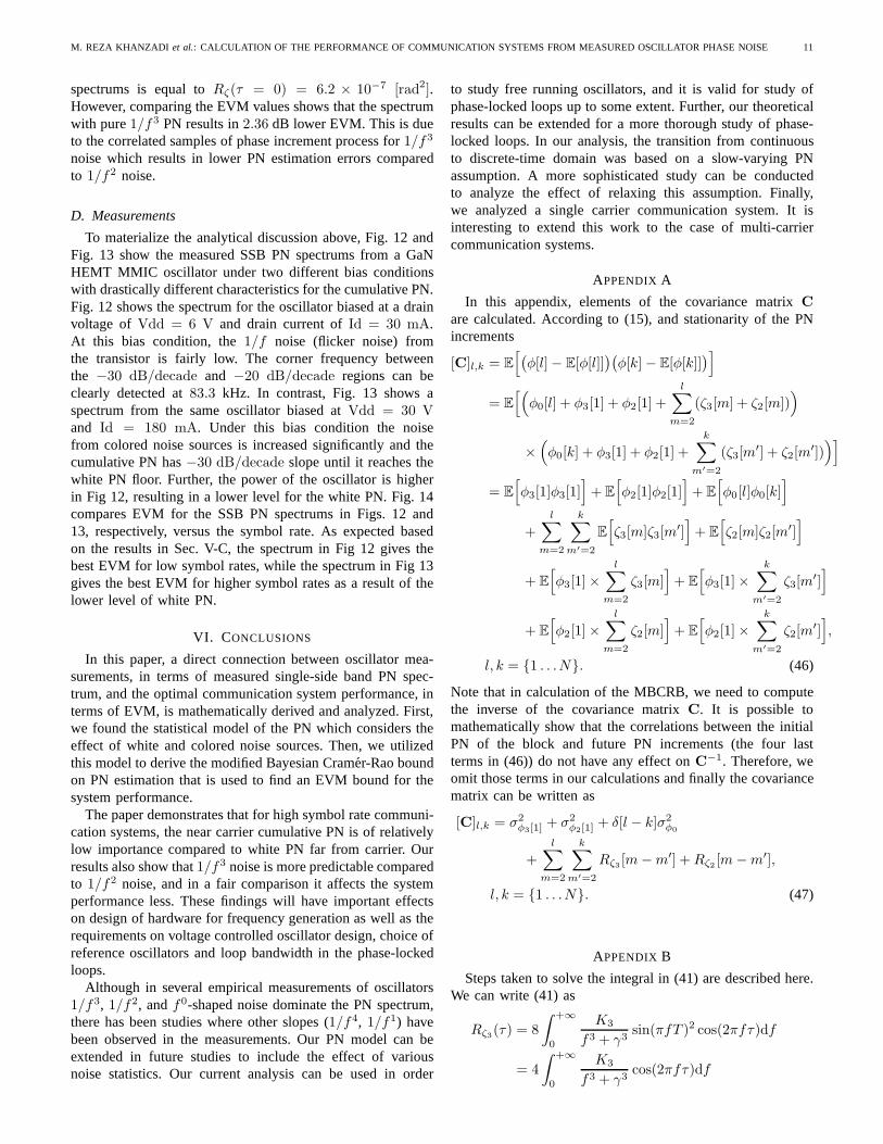
D. Measurements

To materialize the analytical discussion above, Fig. 12 andFig. 13 show the measured SSB PN spectrums from a GaNHEMT MMIC oscillator under two different bias conditionswith drastically different characteristics for the cumulative PN.Fig. 12 shows the spectrum for the oscillator biased at a drainvoltage ofVdd = 6 V and drain current ofId = 30 mA.At this bias condition, the1/f noise (flicker noise) fromthe transistor is fairly low. The corner frequency betweenthe −30 dB/decade and −20 dB/decade regions can beclearly detected at83.3 kHz. In contrast, Fig. 13 shows aspectrum from the same oscillator biased atVdd = 30 Vand Id = 180 mA. Under this bias condition the noisefrom colored noise sources is increased significantly and thecumulative PN has−30 dB/decade slope until it reaches thewhite PN floor. Further, the power of the oscillator is higherin Fig 12, resulting in a lower level for the white PN. Fig. 14compares EVM for the SSB PN spectrums in Figs. 12 and13, respectively, versus the symbol rate. As expected basedon the results in Sec. V-C, the spectrum in Fig 12 gives thebest EVM for low symbol rates, while the spectrum in Fig 13gives the best EVM for higher symbol rates as a result of thelower level of white PN.

VI. CONCLUSIONS

In this paper, a direct connection between oscillator mea-surements, in terms of measured single-side band PN spec-trum, and the optimal communication system performance, interms of EVM, is mathematically derived and analyzed. First,we found the statistical model of the PN which considers theeffect of white and colored noise sources. Then, we utilizedthis model to derive the modified Bayesian Cramer-Rao boundon PN estimation that is used to find an EVM bound for thesystem performance.

The paper demonstrates that for high symbol rate communi-cation systems, the near carrier cumulative PN is of relativelylow importance compared to white PN far from carrier. Ourresults also show that1/f3 noise is more predictable comparedto 1/f2 noise, and in a fair comparison it affects the systemperformance less. These findings will have important effectson design of hardware for frequency generation as well as therequirements on voltage controlled oscillator design, choice ofreference oscillators and loop bandwidth in the phase-lockedloops.

Although in several empirical measurements of oscillators1/f3, 1/f2, andf0-shaped noise dominate the PN spectrum,there has been studies where other slopes (1/f4, 1/f1) havebeen observed in the measurements. Our PN model can beextended in future studies to include the effect of variousnoise statistics. Our current analysis can be used in order

to study free running oscillators, and it is valid for study ofphase-locked loops up to some extent. Further, our theoreticalresults can be extended for a more thorough study of phase-locked loops. In our analysis, the transition from continuousto discrete-time domain was based on a slow-varying PNassumption. A more sophisticated study can be conductedto analyze the effect of relaxing this assumption. Finally,we analyzed a single carrier communication system. It isinteresting to extend this work to the case of multi-carriercommunication systems.

APPENDIX A

In this appendix, elements of the covariance matrixC

are calculated. According to (15), and stationarity of the PNincrements

[C]l,k = E

[(φ[l]− E[φ[l]]

)(φ[k]− E[φ[k]]

)]

= E

[(

φ0[l] + φ3[1] + φ2[1] +

l∑

m=2

(ζ3[m] + ζ2[m]))

×(

φ0[k] + φ3[1] + φ2[1] +

k∑

m′=2

(ζ3[m′] + ζ2[m

′]))]

= E

[

φ3[1]φ3[1]]

+ E

[

φ2[1]φ2[1]]

+ E

[

φ0[l]φ0[k]]

+

l∑

m=2

k∑

m′=2

E

[

ζ3[m]ζ3[m′]]

+ E

[

ζ2[m]ζ2[m′]]

+ E

[

φ3[1]×l∑

m=2

ζ3[m]]

+ E

[

φ3[1]×k∑

m′=2

ζ3[m′]]

+ E

[

φ2[1]×l∑

m=2

ζ2[m]]

+ E

[

φ2[1]×k∑

m′=2

ζ2[m′]]

,

l, k = {1 . . .N}. (46)

Note that in calculation of the MBCRB, we need to computethe inverse of the covariance matrixC. It is possible tomathematically show that the correlations between the initialPN of the block and future PN increments (the four lastterms in (46)) do not have any effect onC−1. Therefore, weomit those terms in our calculations and finally the covariancematrix can be written as

[C]l,k = σ2φ3[1]

+ σ2φ2[1]

+ δ[l − k]σ2φ0

+

l∑

m=2

k∑

m′=2

Rζ3 [m−m′] +Rζ2 [m−m′],

l, k = {1 . . .N}. (47)

APPENDIX B

Steps taken to solve the integral in (41) are described here.We can write (41) as

Rζ3(τ) = 8

∫ +∞

0

K3

f3 + γ3sin(πfT )2 cos(2πfτ)df

= 4

∫ +∞

0

K3

f3 + γ3cos(2πfτ)df

12 IEEE TRANSACTIONS ON CIRCUITS AND SYSTEMS-I: REGULAR PAPERS, 2013

− 2

∫ +∞

0

K3

f3 + γ3cos(2πf(|τ + T |)df

− 2

∫ +∞

0

K3

f3 + γ3cos(2πf(|τ − T |)df. (48)

It is clear that solving the integral in the form of∫ +∞

0 K3/(f3 + γ3) cos(2πfτ)df is enough to compute the

total integral of (48). This integral is complicated enoughthat powerful software such as Mathematica are not ableto converge to the final answer. Consequently, first, partial-fraction decomposition of1/(f3 + γ3) is done:

1

f3 + γ3=

A

f − (−γ)+

B

f − γejπ/3+

C

f − γe−jπ/3

A =1

3γ2, B =

e−j2π/3

3γ2, C =

ej2π/3

3γ2(49)

Note that,γ is a real positive number. Using Mathematica(Version 7.0), the following integral can be evaluated∫ +∞

0

1

f + βcos(2πfτ)df =

− cos(2βπτ)cosint(−2βπ|τ |)

− 1

2sin(2βπ|τ |)(π + 2 sinint(2βπ|τ |)), (50)

whereβ must be a complex or a negative real number, andsinint(·) andcosint(·) are sine and cosine integrals define as

sinint(x) =

∫ r

0

sin(t)

tdt

cosint(x) = Γ + log(x) +

∫ x

0

cos(t)− 1

tdt, (51)

whereΓ ≈ 0.5772 is the Euler-Mascheroni’s constant.Consider the case where time lagτ is small. By Taylor

expansion of the functions in (50) around zero

sin(x) = x− x3

6+ . . . cos(x) = 1− x2

2+ . . .

sinint(x) = x− x3

18+ . . . cosint(x) = Γ + log(x) − x2

4+ . . . ,

and neglecting the terms after second order, the integral canbe approximated as

∫ +∞

0

1

f + βcos(2πfτ)df ≈

− Γ− log(−2βπ|τ |)− 2βπ2|τ |

+(2βπ|τ |)2

2(Λ + log(−2βπ|τ |)), (52)

whereΛ , Γ − 32 . Employing this approximation and the

fraction decomposition in (49), followed by a series of sim-plifications∫ +∞

0

K3

f3 + γ3cos(2πfτ)df ≈

K3

3γ2

(2π√3+ 6γ2π2τ2(Λ + log(2γπ|τ |))

)

. (53)

Now the first term in (48) is calculated. By changing thevariableτ to τ + T and τ − T , second and third terms can

also be computed, respectively. Finally,Rζ3 is approximatedby

Rζ3(τ) ≈− 8K3π2[

− τ2(Λ + log(2πγ|τ |))

+(τ + T )2

2(Λ + log(2πγ|τ + T |))

+(τ − T )2

2(Λ + log(2πγ|τ − T |))

]

. (54)

To calculate the ACF forτ = 0, andτ = |T |, we need to takethe limits of (54) asτ approaches0, and|T |, respectively thatresults in

limτ→0

Rζ3(τ) ≈ −8K3π2T 2(Λ + log(2πγT )), (55)

limτ→|T |

Rζ3(τ) ≈ −8K3π2T 2(Λ + log(8πγT )). (56)

REFERENCES

[1] D. Harris, “Selective demodulation,”Proc. IRE, vol. 35, no. 6, pp. 565– 572, Jun. 1947.

[2] A. Viterbi, “Phase-locked loop dynamics in the presenceof noise byfokker-planck techniques,”Proc. IEEE, vol. 51, no. 12, pp. 1737 – 1753,Dec. 1963.

[3] T. Pollet, M. Van Bladel, and M. Moeneclaey, “BER sensitivity ofOFDM systems to carrier frequency offset and Wiener phase noise,”IEEE Trans. Commun., vol. 43, no. 234, pp. 191 –193, Feb./Mar./Apr.1995.

[4] U. Mengali and M. Morelli, “Data-aided frequency estimation for burstdigital transmission,”IEEE Trans. Commun., vol. 45, no. 1, pp. 23 –25,Jan. 1997.

[5] H. Meyr, M. Moeneclaey, and S. Fechtel,Digital CommunicationReceivers: Synchronization, Channel Estimation, and Signal Processing.New York, NY, USA: John Wiley & Sons, Inc., 1997.

[6] L. Tomba, “On the effect of Wiener phase noise in OFDM systems,”IEEE Trans. Commun., vol. 46, no. 5, pp. 580 –583, 1998.

[7] A. Armada and M. Calvo, “Phase noise and sub-carrier spacing effectson the performance of an OFDM communication system,”IEEE Com-mun. Lett., vol. 2, no. 1, pp. 11 –13, 1998.

[8] A. Armada, “Understanding the effects of phase noise in orthogonalfrequency division multiplexing (OFDM),”IEEE Trans. Broadcast.,vol. 47, no. 2, pp. 153 –159, Jun. 2001.

[9] P. Amblard, J. Brossier, and E. Moisan, “Phase tracking:what do we gainfrom optimality? particle filtering versus phase-locked loops,” ElsevierSignal Process., vol. 83, no. 1, pp. 151 – 167, Mar. 2003.

[10] F. Munier, E. Alpman, T. Eriksson, A. Svensson, and H. Zirath, “Es-timation of phase noise for QPSK modulation over AWGN channels,”Proc. GigaHertz 2003 Symp.,Linkoping, Sweden, Nov. 2003.

[11] H. Zirath, T. Masuda, R. Kozhuharov, and M. Ferndahl, “Developmentof 60-ghz front-end circuits for a high-data-rate communication system,”IEEE J. Solid-State Circuits, vol. 39, no. 10, pp. 1640 – 1649, Oct. 2004.

[12] S. Wu and Y. Bar-Ness, “OFDM systems in the presence of phase noise:consequences and solutions,”IEEE Trans. Commun., vol. 52, no. 11, pp.1988 – 1996, Nov. 2004.

[13] D. Baum and H. Bolcskei, “Impact of phase noise on MIMO channelmeasurement accuracy,”Vehicular Tech. Conf. (VTC), vol. 3, pp. 1614– 1618, Sep. 2004.

[14] J. Dauwels and H.-A. Loeliger, “Phase estimation by message passing,”in Proc. IEEE Int. Conf. Commun., Jun. 2004.

[15] E. Panayırı, H. Cırpan, and M. Moeneclaey, “A sequential monte carlomethod for blind phase noise estimation and data detection,” in Proc.13th European Signal Process. Conf. EUSIPCO, Sep. 2005.

[16] G. Colavolpe, A. Barbieri, and G. Caire, “Algorithms for iterativedecoding in the presence of strong phase noise,”IEEE J. Sel. AreasCommun., vol. 23, pp. 1748–1757, Sep. 2005.

[17] F. Munier, T. Eriksson, and A. Svensson, “An ICI reduction schemefor OFDM system with phase noise over fading channels,”IEEE Trans.Commun., vol. 56, no. 7, pp. 1119 –1126, 2008.

M. REZA KHANZADI et al.: CALCULATION OF THE PERFORMANCE OF COMMUNICATION SYSTEMS FROM MEASURED OSCILLATOR PHASE NOISE 13

[18] T. Pedersen, X. Yin, and B. Fleury, “Estimation of MIMO channel capac-ity from phase-noise impaired measurements,”IEEE Global Commun.Conf. (GLOBECOM), pp. 1 –6, Dec. 2008.

[19] M. Nissila and S. Pasupathy, “Adaptive iterative detectors for phase-uncertain channels via variational bounding,”IEEE Trans. Commun.,vol. 57, no. 3, pp. 716 –725, Mar. 2009.

[20] J. Bhatti and M. Moeneclaey, “Feedforward data-aided phase noiseestimation from a DCT basis expansion,”EURASIP J. Wirel. Commun.Netw., Jan. 2009.

[21] M. Dohler, R. Heath, A. Lozano, C. Papadias, and R. Valenzuela, “Isthe PHY layer dead?”IEEE Commun. Mag., vol. 49, no. 4, pp. 159–165, Apr. 2011.

[22] R. Krishnan, H. Mehrpouyan, T. Eriksson, and T. Svensson, “Optimaland approximate methods for detection of uncoded data with carrierphase noise,”IEEE Global Commun. Conf. (GLOBECOM), pp. 1 –6,Dec. 2011.

[23] R. Krishnan, M.R. Khanzadi, L. Svensson, T. Eriksson, and T. Svensson,“Variational bayesian framework for receiver design in thepresence ofphase noise in MIMO systems,”IEEE Wireless Commun. and Netw.Conf. (WCNC), pp. 1 –6, Apr. 2012.

[24] H. Mehrpouyan, A. A. Nasir, S. D. Blostein, T. Eriksson,G. K. Kara-giannidis, and T. Svensson, “Joint estimation of channel and oscillatorphase noise in MIMO systems,”IEEE Trans. Signal Process., vol. 60,no. 9, pp. 4790 –4807, Sep. 2012.

[25] G. Durisi, A. Tarable, C. Camarda, and G. Montorsi, “On the capacityof MIMO Wiener phase-noise channels,”Proc. Inf. Theory Applicat.Workshop (ITA), Feb. 2013.

[26] R. Krishnan, M.R. Khanzadi, T. Eriksson, and T. Svensson, “Softmetrics and their performance analysis for optimal data detection inthe presence of strong oscillator phase noise,”IEEE Trans. Commun.,vol. 61, no. 6, pp. 2385 –2395, Jun. 2013.

[27] M. Martalo, C. Tripodi, and R. Raheli, “On the information rate of phasenoise-limited communications,”Proc. Inf. Theory Applicat. Workshop(ITA), Feb. 2013.

[28] H. Ghozlan and G. Kramer, “On Wiener phase noise channels at highsignal-to-noise ratio,”arXiv preprint arXiv:1301.6923, 2013.

[29] ——, “Multi-sample receivers increase information rates for Wienerphase noise channels,”arXiv preprint arXiv:1303.6880, 2013.

[30] M.R. Khanzadi, R. Krishnan, and T. Eriksson, “Effect ofsynchroniz-ing coordinated base stations on phase noise estimation,”Proc. IEEEAcoust., Speech, Signal Process. (ICASSP), May. 2013.

[31] S. Bay, C. Herzet, J.-M. Brossier, J.-P. Barbot, and B. Geller, “Analyticand Asymptotic Analysis of Bayesian Cramer Rao Bound for DynamicalPhase Offset Estimation,”IEEE Trans. Signal Process., vol. 56, no. 1,pp. 61 –70, Jan. 2008.

[32] Z. Chen and F. Dai, “Effects of LO phase and amplitude imbalancesand phase noise on M-QAM transceiver performance,”IEEE Trans.Ind. Electron., vol. 57, no. 5, pp. 1505 –1517, May. 2010.

[33] A. Georgiadis, “Gain, phase imbalance, and phase noiseeffects on errorvector magnitude,”IEEE Trans. Veh. Technol., vol. 53, no. 2, pp. 443 –449, Mar. 2004.

[34] A. Demir, “Computing timing jitter from phase noise spectra foroscillators and phase-locked loops with white and1/f noise,” IEEETrans. Circuits Syst. I, Reg. Papers, vol. 53, no. 9, pp. 1869 –1884, Sep.2006.

[35] M.R. Khanzadi, H. Mehrpouyan, E. Alpman, T. Svensson, D. Kuylen-stierna, and T. Eriksson, “On models, bounds, and estimation algorithmsfor time-varying phase noise,”Int. Conf. Signal Process. Commun. Syst.(ICSPCS), pp. 1 –8, Dec. 2011.

[36] A. Demir, “Phase noise and timing jitter in oscillatorswith colored-noisesources,”IEEE Trans. Circuits Syst. I, Fundam. Theory Appl., vol. 49,no. 12, pp. 1782 – 1791, Dec. 2002.

[37] M.R. Khanzadi, A. Panahi, D. Kuylenstierna, and T. Eriksson, “A model-based analysis of phase jitter in RF oscillators,”IEEE Intl. FrequencyControl Symp. (IFCS), pp. 1 –4, May 2012.

[38] S. Yousefi and J. Jalden, “On the predictability of phasenoise modeledas flicker FM plus white FM,”Proc. Asilomar Conf., pp. 1791 –1795,Nov. 2010.

[39] D. Leeson, “A simple model of feedback oscillator noisespectrum,”Proc. IEEE, vol. 54, no. 2, pp. 329 – 330, 1966.

[40] J. McNeill, “Jitter in ring oscillators,” IEEE J. Solid-State Circuits,vol. 32, no. 6, pp. 870 –879, Jun. 1997.

[41] F. Herzel, “An analytical model for the power spectral density ofa voltage-controlled oscillator and its analogy to the laser linewidththeory,” IEEE Trans. Circuits Syst. I, Fundam. Theory Appl., vol. 45,no. 9, pp. 904 –908, 1998.

[42] A. Hajimiri and T. Lee, “A general theory of phase noise in electricaloscillators,” IEEE J. Solid-State Circuits, vol. 33, no. 2, pp. 179 –194,1998.

[43] A. Hajimiri, S. Limotyrakis, and T. Lee, “Jitter and phase noise in ringoscillators,” IEEE J. Solid-State Circuits, vol. 34, no. 6, pp. 790 –804,Jun. 1999.

[44] G. Klimovitch, “Near-carrier oscillator spectrum dueto flicker and whitenoise,” Proc. IEEE Intl. Symp. on Circuits Systs., vol. 1, pp. 703 –706vol.1, May 2000.

[45] ——, “A nonlinear theory of near-carrier phase noise in free-runningoscillators,” Proc. IEEE Intl. Conf. on Circuits Systs., pp. 1 –6, 2000.

[46] A. Demir, A. Mehrotra, and J. Roychowdhury, “Phase noise in oscil-lators: a unifying theory and numerical methods for characterization,”IEEE Trans. Circuits Syst. I, Fundam. Theory Appl., vol. 47, no. 5, pp.655 –674, May 2000.

[47] C. Liu and J. McNeill, “Jitter in oscillators with1/f noise sources,”Proc. IEEE 2004 Intl. Symp. on Circuits Systs., vol. 1, pp. 773–776,May. 2004.

[48] A. A. Abidi, “Phase noise and jitter in CMOS ring oscillators,” IEEEJ. Solid-State Circuits, vol. 41, no. 8, pp. 1803–1816, Aug. 2006.

[49] A. Chorti and M. Brookes, “A spectral model for RF oscillators withpower-law phase noise,”IEEE Trans. Circuits Syst. I, Reg. Papers,vol. 53, no. 9, pp. 1989 –1999, 2006.

[50] H. Wang, K.-W. Chang, D.-W. Lo, L. Tran, J. Cowles, T. Block, G. S.Dow, A. Oki, D. Streit, and B. Allen, “A 62-GHz monolithic InP-basedHBT VCO,” IEEE Microw. Guided Wave Lett., vol. 5, no. 11, pp. 388–390, Nov. 1995.

[51] S. Gunnarsson, C. Karnfelt, H. Zirath, R. Kozhuharov, D. Kuylenstierna,A. Alping, and C. Fager, “Highly integrated 60 GHz transmitter andreceiver MMICs in a GaAs pHEMT technology,”IEEE J. Solid-StateCircuits, vol. 40, no. 11, pp. 2174 – 2186, Nov. 2005.

[52] T. Decker and R. Temple, “Choosing a phase noise measurementtechnique,”RF and Microwave Measurement Symposium and Exhibition,1999.

[53] J. McNeill, “Jitter in ring oscillators,” Ph.D. dissertation, Boston Uni-versity, 1994.

[54] K. Kundert, “Predicting the phase noise and jitter of PLL-based frequency synthesizers,” 2003, [Online]. Available:http://designers-guide.com.

[55] C. Liu, “Jitter in oscillators with1/f noise sources and application totrue RNG for cryptography,” Ph.D. dissertation, WorcesterPolytechnicInstitute, 2006.

[56] A. Murat, P. Humblet, and J. Young, “Phase-noise-induced performancelimits for DPSK modulation with and without frequency feedback,” J.Lightw. Technol., vol. 11, no. 2, pp. 290 –302, Feb. 1993.

[57] J. G. Proakis and M. Salehi,,Digital communications, 5th ed. NewYork: McGraw-Hill, 2008.

[58] R. Hassun, M. Flaherty, R. Matreci, and M. Taylor, “Effective evaluationof link quality using error vector magnitude techniques,”Proc. WirelessCommun. Conf., pp. 89 –94, Aug. 1997.

[59] T. Nakagawa and K. Araki, “Effect of phase noise on RF communicationsignals,” Veh. Technol. Conf. (VTC), vol. 2, pp. 588 –591 vol.2, Sep.2000.

[60] S. M. Kay, Fundamentals of Statistical Signal Processing, EstimationTheory. Prentice Hall, Signal Processing Series, 1993.

[61] H. L. V. Trees, Detection, Estimation and Modulation Theory.New York: Wiley, 1968, vol. 1.

[62] A. D’Andrea, U. Mengali, and R. Reggiannini, “The modified Cramer-Rao bound and its application to synchronization problems,” IEEE Trans.Commun., vol. 42, no. 234, pp. 1391 –1399, Feb.-Mar.-Apr. 1994.

[63] R. Corvaja and S. Pupolin, “Effects of phase noise spectral shapeon the performance of DPSK systems for wireless applications,” Eur.Trans. Telecommun. (ETT), vol. 13, no. 3, pp. 203–210, May. 2002.[Online]. Available: http://dx.doi.org/10.1002/ett.4460130305

[64] J. Havil, Gamma: exploring Euler’s constant. Princeton, NJ: PrincetonUniversity Press, 2003.

[65] N. Kasdin, “Discrete simulation of colored noise and stochastic pro-cesses and1/fα; power law noise generation,”Proc. IEEE, vol. 83,no. 5, pp. 802 –827, May 1995.

[66] S. Yousefi, T. Eriksson, and D. Kuylenstierna, “A novel model forsimulation of RF oscillator phase noise,”IEEE Radio and Wireless Symp.(RWS), pp. 428 –431, Jan. 2010.

[67] M.R. Khanzadi, R. Krishnan, and T. Eriksson, “Estimation of phasenoise in oscillators with colored noise sources,”IEEE Commun. Lett.,vol. 17, no. 11, pp. 2160 –2163, Sep. 2013.