IEEE TRANSACTIONS ON AFFECTIVE COMPUTING, VOL. PP, NO. 99, DEC 2017 1

Personalized Multitask Learning for PredictingTomorrow’s Mood, Stress, and HealthSara Taylor∗, Student Member, IEEE, Natasha Jaques∗, Student Member, IEEE,Ehimwenma Nosakhare, Student Member, IEEE, Akane Sano, Member, IEEE,

and Rosalind Picard, Fellow, IEEE

Abstract—While accurately predicting mood and wellbeing could have a number of important clinical benefits, traditional machinelearning (ML) methods frequently yield low performance in this domain. We posit that this is because a one-size-fits-all machinelearning model is inherently ill-suited to predicting outcomes like mood and stress, which vary greatly due to individual differences.Therefore, we employ Multitask Learning (MTL) techniques to train personalized ML models which are customized to the needs ofeach individual, but still leverage data from across the population. Three formulations of MTL are compared: i) MTL deep neuralnetworks, which share several hidden layers but have final layers unique to each task; ii) Multi-task Multi-Kernel learning, which feedsinformation across tasks through kernel weights on feature types; and iii) a Hierarchical Bayesian model in which tasks share acommon Dirichlet Process prior. We offer the code for this work in open source. These techniques are investigated in the context ofpredicting future mood, stress, and health using data collected from surveys, wearable sensors, smartphone logs, and the weather.Empirical results demonstrate that using MTL to account for individual differences provides large performance improvements overtraditional machine learning methods and provides personalized, actionable insights.

Index Terms—Mood Prediction, Multitask learning, Deep Neural Networks, Multi-Kernel SVM, Hierarchical Bayesian Model

F

1 INTRODUCTION

P ERCEIVED wellbeing, as measured by self-reportedhealth, stress, and happiness, has a number of im-

portant clinical health consequences. Self-reported happi-ness is not only indicative of scores on clinical depressionmeasures [1], but happiness is so strongly associated withgreater longevity that the effect size is comparable to thatof cigarette smoking [2]. Stress increases susceptibility toinfection and illness [3]. Finally, self-reported health is sostrongly related to actual health and all-cause mortality [4],that in a 29-year-study it was found to be the single mostpredictive measure of mortality, above even more objectivehealth measures such as blood pressure readings [5].

Clearly, the ability to model and predict subjective moodand wellbeing could be immensely beneficial, especially ifsuch predictions could be made using data collected in anunobtrusive and privacy-sensitive way, perhaps using wear-able sensors and smartphones. Such a model could open upa range of beneficial applications which passively monitorusers’ data and make predictions about their mental andphysical wellbeing. This could not only aid in the manage-ment, treatment, and prevention of both mental illness anddisease, but the predictions could be useful to any personwho might want a forecast of their future mood, stress,or health in order to make adjustments to their routine toattempt to improve it. For example, if the model predicts

• S. Taylor, N. Jaques, A. Sano and R. Picard are with the Program of MediaArts and Sciences and the MIT Media Lab.E-mail: sataylor, jaquesn, akanes, picard@media.mit.edu

• E. Nosakhare is with the Department of Electrical Engineering andComputer Science and the MIT Media Lab. E-mail: ehinosa@mit.edu

∗Both authors contributed equally to this workManuscript received June 28, 2017; revised Nov 2, 2017; Accepted Dec 2 2017.

that I will be extremely stressed tomorrow, I might want tochoose a different day to agree to review that extra paper.

Unfortunately, modeling wellbeing and mood is an in-credibly difficult task, and a highly accurate, robust systemhas yet to be developed. Historically, classification accu-racies have ranged from 55-80% (e.g., [6]–[8]), even withsophisticated models or multi-modal data. In this paper, weuse a challenging dataset where accuracies from prior effortsto recognize wellbeing and mood ranged from 56-74% [9],[10]. Across many mood detection systems, performanceremains low despite researchers’ considerable efforts todevelop better models and extract meaningful features froma diverse array of data sources.

We hypothesize that these models suffer from a commonproblem: the inability to account for individual differences.What puts one person in a good mood does not apply toeveryone else. For instance, the stress reaction experiencedby an introvert during a loud, crowded party might bevery different for an extrovert [11]. Individual differencesin personality can strongly affect mood and vulnerability tomental health issues such as depression [12]. There are evenindividual differences in how people’s moods are affectedby the weather [13]. Thus, a generic, omnibus machinelearning model trained to predict mood is inherently limitedin the performance it can obtain.

We show that accounting for interindividual variabilityvia MTL can dramatically improve the prediction of thesewellbeing states: mood, stress, and health. MTL is a typeof transfer learning, in which models are learned simul-taneously for several related tasks, but share informationthrough similarity constraints [14]. We show that MTL canallow each person to have a model tailored specifically forthem, which still learns from all available data. Therefore,

IEEE TRANSACTIONS ON AFFECTIVE COMPUTING, VOL. PP, NO. 99, DEC 2017 2

the approach remains feasible even if there is insufficientdata to train an individual machine learning model for eachperson. By adapting existing MTL methods to account forindividual differences in the relationship between behaviorand wellbeing, we are able to obtain state-of-the-art perfor-mance on the dataset under investigation (78-82% accuracy),significantly improving on prior published results.

In addition to showing the benefits of personalization,we undertake a more challenging task than is typically at-tempted when modeling mood. While most prior work hasfocused on detecting current mood state, we test the abilityto predict mood and wellbeing tomorrow night (at least 20hours in the future), using only data from today. Specifically,assume xt represents all the smartphone, wearable sensor,and weather data collected about a person on day t (from12:00am to 11:59pm). Let yt be the person’s self-reportedmood, stress, and health in the evening of day t (reportedafter 8pm). Previous work has focused on learning to modelp(yt|xt); that is, the probability of the person’s currentmood given the current data, which we refer to as mooddetection. In contrast, we learn p(yt+1|xt), the probability ofthe person’s mood tomorrow given today’s data. This typeof prediction could be considered a type of mood forecasting,providing an estimate of a person’s future wellbeing whichcould potentially allow them to better prepare for it — justas a weather forecast gives one a chance to take an umbrellarather than being left to be soaked by the rain.

Typical forecasting models make use of a history of priorlabels to make predictions; i.e. such models learn the func-tion p(yt+1|yt, yt−1, . . . , y1, xt, xt−1, . . . , x1). Using such amodel for mood forecasting is less than desirable, since itimplies that a person must input their mood every day inorder to obtain predictions about tomorrow. In contrast, wedo not use any prior labels. Instead, we learn p(yt+1|xt),allowing us to predict an individual’s mood without everrequiring them to manually input a mood rating.

Our work makes the following contributions to the af-fective computing literature. We predict future wellbeingwithout requiring a history of collected wellbeing labels foreach person. Our data are gathered in the “wild” as partic-ipants go about their daily lives, using surveys, wearablesensors, weather monitoring, and smartphones, and thusare relevant to use in a real-world wellbeing predictionsystem. We provide insights into the relationship betweenthe collected data and mood and wellbeing, through animplicit soft clustering of users provided by the Bayesianmodel, and a learned weighting of input sources. Finally, wedemonstrate the ability of MTL to train personalized modelsthat can account for individual differences, and provide thedeveloped code for the MTL models in open source. Theinsight that personalization through MTL can significantlyimprove mood prediction performance could be a valuablestep towards developing a practical, deployable mood pre-diction system.

2 RELATED WORK

The idea of estimating mood, stress, and mental health indi-cators using unobtrusive data collected from smartphonesand wearables has been garnering increasing interest. Forexample, Bogomolov and colleagues [15] use smartphone

data combined with information about participants’ per-sonalities and the weather to detect stress with 72% accu-racy. Other researchers have investigated using smartphonemonitoring to detect depressive and manic states in bipolardisorder, attaining accuracy of 76% [8]. Detecting workplacestress is another growing body of research [16].

The insight that an impersonal, generic affect classifiercannot account for individual differences has been arrivedat by several researchers. In estimating workplace stress,Koldijk and colleagues found that adding the participant IDas a feature to their model could improve accuracy in classi-fying mental effort [17]. Similarly, Canzian and colleaguesfound that training a generic SVM to classify depressivemood from location data and surveys resulted in sensitivityand specificity values of 0.74 and 0.78, respectively. Bytraining an independent SVM for each person, the authorsobtained values of 0.71 and 0.87 [18].

Finally, a detailed study reported that an omnibus modeltrained to detect all people’s mood based on smartphonecommunication and usage resulted in a prediction accuracyof 66% [7]. However, if two months of labeled data werecollected for each person, then individual, independentpersonalized models could be trained to achieve 93% ac-curacy in mood classification! Since obtaining two monthsof training data per person can be considered somewhatunrealistic, the authors investigated methods for traininga hybrid model that weights personalized examples moreheavily, which can be used when there are fewer labeledtraining examples per person. In contrast with this workwe focus on methods for making reasonable personalizedpredictions even in the absence of any labeled training datafor a new person.

As mentioned above, almost all prior work of whichwe are aware has focused on mood detection, rather thantrue prediction; that is, learning p(yt|xt), where the modellabel yt and data xt are both collected on day t. A recentpaper published in April 2017 claims to be the first workto forecast future mood [19]. This work uses a RecurrentNeural Network (RNN) to predict mood given two weeksof mood history reported every day, learning the func-tion p(yt+1|yt, yt−1...y1, xt, xt−1...x1). Using a large-scaledataset of 2,382 people, the authors achieved an AUC scoreof 0.886 in forecasting severely depressed mood. While anotable contribution, the drawback to this approach is thatit requires a person to diligently input their mood every day.If one day is missed, a prediction cannot be made for thenext two weeks. Further, the results reveal that past moodfeatures are many times more effective at predicting futuremood than any of the other data collected. Thus, using amood history to predict future mood is a significantly easierproblem. In contrast, we are able to predict tomorrow’swellbeing given a rich set of data from today (p(yt+1|xt)),obtaining accurate predictions about an individual’s futuremood through personalization, without requiring them tomanually input self-reported labels.

2.1 Multitask Learning

MTL is a type of transfer learning, in which models arelearned simultaneously for several tasks but share informa-tion through similarity constraints. Originally proposed as a

IEEE TRANSACTIONS ON AFFECTIVE COMPUTING, VOL. PP, NO. 99, DEC 2017 3

way to induce efficient internal representations within neu-ral networks (NNs) [14], MTL can be used across a varietyof models. It can be considered a form of regularization,and can improve generalization performance [14] as long astasks are sufficiently related [20]. Because MTL is beneficialwhen training data is scarce and noisy, it is well-suited tothe messy, real-world problem of predicting mood.

Since Caruana’s original work, a variety of NN MTLmethods have been explored. For example, face detectionaccuracy for a deep convolutional network can be improvedby sharing layers with networks trained on similar tasks,like face pose estimation and facial landmark localization[21]. Multitasking has also been used successfully to trainNNs with very little data; by using the same network topredict traffic flow in the past, present, and future, Jin andSun were able to improve prediction accuracies using only2112 samples of traffic data [22].

Hierarchical Bayesian learning is a popular approach toMTL; Baxter and colleagues provide a detailed overview[23]. The general approach is exemplified by an algorithmlike Transfer-Aware Naive Bayes [20]: each task’s model’sparameters are drawn from a common prior distribution,thus imposing a similarity constraint. The model can updatethe parameters of the prior as it learns — for example, by de-creasing the variance if the tasks are very similar. Bayesianinference techniques have been applied to a number of MTLscenarios. For example, MTL has been applied to a reinforce-ment learning problem in which each task is an environmentan agent must explore, and the Markov Decision Process(MDP) learned for previous environments is treated as astrong prior on the model for a new environment [24].

MTL has also been explored within the Affective Com-puting community. The idea of treating predicting the affectof a single person as a task was introduced in conjunctionwith Multi-Task Multi-Kernel Learning (MTMKL) [25] usingthe DEAP dataset [26]. MTMKL is an MTL method specifi-cally designed for Affective Computing applications whichneed to combine data from multiple disparate sources,or modalities [25]. A kernel function is computed usingthe features from each modality, and these are combinedin a weighted sum. MTL is applied by learning separatekernel weights for each task, while constraining all tasks’weights to be similar. Thus, information is shared acrosstasks through the kernel weights on the modalities [25].While treating modeling different people as related tasksin MTMKL allows for personalization, it does not allow themodel to generalize to a new person. In contrast, we firstcluster people based on personality and treat predicting thewellbeing of a cluster as a task, allowing us to generalize tonew users who have not input wellbeing labels by placingthem into the appropriate cluster.

MTL can also be applied to Affective Computing bytreating outcomes like arousal and valence as the relatedtasks in the model. This method was used in our prior work,which applied MTMKL to the dataset under investigation inthis paper by treating the classification of happiness, stress,health, alertness, and energy as related tasks [10]. Similarly,Xia and colleagues improved the performance of a deep be-lief network by training it to simultaneously recognize bothvalence and arousal from speech [27]. In another study ofspeech emotion recognition, the authors found that treating

different corpora, domains, or genders as related tasks in anMTL framework offered performance benefits over learninga single model over all of the domains, or learning a separatemodel for each domain [28].

3 METHODS

In what follows we describe several techniques for us-ing MTL to account for interindividual differences in therelationship between behavior, physiology, and resultingmood and wellbeing. Each of the models can adapt to thespecific characteristics of each person, while still sharinginformation across people through a) shared layers of a deepneural network (Section 3.1); b) a similarity constraint oneach task’s classifier’s weights (Section 3.2); or c) a commonprior shared across tasks (Section 3.3)

The most intuitive way to use MTL to customize a modelfor each person is to treat predicting the wellbeing of asingle person as a single task. However, this approach maybecome untenable if there are few samples per person. Sinceit requires that each person have a unique, fully trained,task-specific model, each person would need to provide asufficient amount of labeled data. This may constitute a dis-incentivizing burden on potential users. More importantly,such a model cannot generalize to new people or make accuratepredictions about new users.

Therefore, we begin by clustering users based on theirpersonality and gender, and treat predicting mood for agiven cluster as one prediction task. In this way, we caneasily make predictions for a new user without requiringthem to input their mood on a daily basis; we simply usetheir personality and gender to assign them to the appro-priate cluster. In this study, personality is computed usingthe Big Five trait taxonomy [29], via a questionnaire thattakes approximately 10 minutes to complete. We apply K-means clustering to participants’ Big Five scores and gender,and assess cluster quality in an unsupervised way usingsilhouette score, which is evaluated based on the intra-clusterand nearest-cluster distance for each sample [30]. The num-ber of clusters which produced the highest silhouette scorewas K = 37. Using a large number of clusters allows usto create fine-grained, highly customized models that makemood predictions for extremely specific types of people.

3.1 Neural Networks

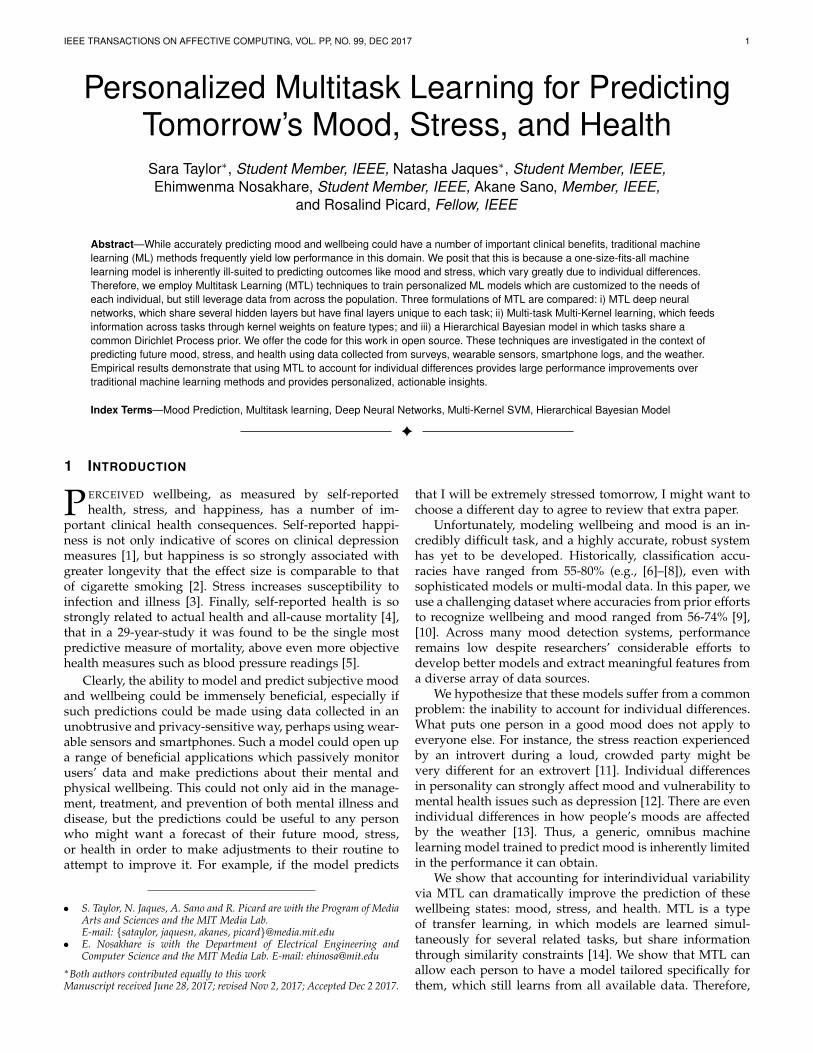
To build a MTL neural network (NN), we begin with severalinitial hidden layers that are shared among all the tasks.These layers then connect to smaller, task-specific layers,which are unique to each cluster. Figure 1 shows a simplifiedversion of this architecture. In reality, the network can havemany shared and task-specific layers.

The intuition behind this design is that the sharedlayers will learn to extract information that is useful forsummarizing relevant characteristics of any person’s dayinto an efficient, generalizable embedding. The final, task-specific layers are then expected to learn how to map thisembedding to a prediction customized for each cluster. Forexample, if the shared layers learn to condense all of therelevant smartphone app data about phone calls and textinginto an aggregate measure of social support, the task-specific

IEEE TRANSACTIONS ON AFFECTIVE COMPUTING, VOL. PP, NO. 99, DEC 2017 4

Fig. 1: A simplified version of the MTL-NN architecture.Clusters of related people receive specialized predictionsfrom a portion of the network trained with only their data.Shared initial layers extract features relevant to all clusters.

layers can then learn a unique weighting of this measure foreach cluster. Perhaps a cluster containing participants withhigh extroversion scores will be more strongly affected by alack of social support than another cluster.

To train the network, we must slightly modify the typicalStochastic Gradient Descent (SGD) algorithm. Rather thanrandomly selecting a mini-batch of N training samples fromany of the available data, each mini-batch must only containdata from a single randomly selected task or cluster. Themini-batch is then used to predict label values y′i, basedon forward propagation through the shared weights andthe appropriate cluster-specific weights. The ground-truthtarget labels yi are used to compute the error with respectto that batch using the typical cross-entropy loss function:

LH(Y,Y′) = −N∑i=1

[yi log y′i + (1− yi) log(1− y′i)]

A gradient step based on the loss is then used to updateboth the cluster-specific weights, as well as to adjust theweights within the shared layers. By continuing to ran-domly sample a new cluster and update both the cluster-specific and shared weights, the network will eventuallylearn a shared representation relevant to all clusters.

While deep learning is a powerful branch of ML, whentraining on small datasets such as the one under discussionin this paper it is important to heavily regularize the net-work to avoid overfitting. Although MTL itself is a strongform of regularization, we implement several other tech-niques to ensure generalizable predictions. As is common,we include the following L2 regularization term in the lossfunction: −β‖W‖22, where W are the weights of the net-work. We also train the network to simultaneously predictall three wellbeing labels to further improve the generaliz-ability of the embedding. Finally, we implement dropout,a popular approach to NN regularization in which someportion of the network’s weights are randomly “droppedout” (set to 0) during training. This forces the networkto learn redundant representations and is statistically verypowerful. Using a dropout factor of 0.5 (meaning thereis a 50% chance a given weight will be dropped duringtraining) on a NN with n nodes is equivalent to training 2n

NNs which all share parameters [31]. This is easy to verify;consider a binary variable that represents whether or not a

node is dropped out on a given training iteration. Since thereare n nodes, there are 2n possible combinations of thesebinary variables. Moreover, each of these sub-networks aretrained on different, random mini-batches of data, and thisbagging effect further enhances generalization performance.

3.2 Multi-Task Multi-Kernel Learning

As introduced in Section 2, the MTMKL algorithm devel-oped by Kandemir et. al. [25] is a MTL technique designedfor the problem of classifying several related emotions(tasks) based on multiple data modalities [25]. MTMKLis a modified version of Multi-Kernel Learning (MKL) inwhich tasks share information through kernel weights onthe modalities. Here, we consider the problem of usingMTMKL to build a personalized model that can accountfor individual differences. Therefore, we treat each task aspredicting the wellbeing for one cluster; that is, a groupof highly similar people which share the same gender orpersonality traits.

MTMKL uses a least-squares support vector machine(LSSVM) for each task-specific model. Unlike the canonicalSVM, the LSSVM uses a quadratic error on the “slack”variables instead of an L1 error. As a result, the LSSVM canbe learned by solving a series of linear equations in contrastto using quadratic programing to learn an SVM model. TheLSSVM has the added benefit that when only a single labelis present in the training data, its predictions will default topredict only that label.

The LSSVM can be learned by solving the followingoptimization problem, in which N is the total number ofsamples, xi is the ith feature vector, yi is the ith label,k(xi, xj) is a kernel function, and α is the set of dualcoefficients as in a conventional SVM:

maximizeα

− 1

2

N∑i=1

N∑j=1

αiαjyiyjk(xi, xj)

− 1

2C

N∑i=1

α2i +

N∑i=1

αi

subject toN∑i=1

αiyi = 0

In MKL, we build on the LSSVM by adjusting the kernelfunction. In particular, we use a kernel function to computethe similarity between feature vectors for each modalitym, and the kernels are combined using a weighted sum.The weights depend on the usefulness of each modality inprediction. That is, more useful modalities will have largerkernel weights so that differences in that data modality aremore helpful in prediction.

Concretely, we assign a kernel km to the features inmodality m, as in typical MKL. We restrict the model spaceby using the same kernel function (e.g., an RBF kernel) foreach modality. The modality kernels are combined into asingle kernel, kη , in a convex combination parameterized bythe kernel weighting vector, η. Let x(m)

i be the ith featurevector that contains only the features belonging to modalitym, and M be the total number of modalities. Then kη isdefined as follows:

IEEE TRANSACTIONS ON AFFECTIVE COMPUTING, VOL. PP, NO. 99, DEC 2017 5

kη(xi,xj ;η) =M∑m=1

ηmkm(x(m)i ,x

(m)j )

such that ηm > 0,m = 1, . . . ,M and∑Mm=1 ηm = 1.

Thus the LSSVM-based MKL model can be learned usingthe same optimization as the LSSVM with the additionalconstraint of the convex combination of kernel weights η.

When multiple tasks are learned at the same time inMTMKL, each task t has its own vector of kernel weights,η(t), which are regularized globally by a function whichpenalizes divergence from the weights of the other tasks.This allows information about the kernel weights to beshared between tasks so that each task benefits from thedata of other tasks. In particular, if the model is highlyregularized, then the kernel weight on the mth modality(i.e., η(t)

m ) will be very similar across all tasks t. As such, eachtask will treat the modalities as having similar importance.Note that even though the kernel weights might be highlyregularized, the task-specific models can still learn a diverseset of decision boundaries within the same kernel space.

The optimal η(t) for all tasks t = 1, . . . , T can belearned by solving a min-max optimization similar to theLSSVM-based MKL model, but with the addition of theregularization function, Ω(η(t)Tt=1). A weight ν placed onthe regularization function Ω(·) controls the importance ofthe divergence. When ν = 0 the tasks are treated indepen-dently, and as ν increases, the task weights are increasinglyrestricted to be similar.

For simplicity of notation we denote the objective func-tion for a single task’s LSSVM-based MKL model as follows:

J (t)(α(t),η(t)

)=− 1

2

N(t)∑i=1

N(t)∑j=1

α(t)i α

(t)j yiyjk

(t)η (xi, xj)

− 1

2C

N(t)∑i=1

α2i +

N(t)∑i=1

αi

where the superscript (t) denotes the parameters or func-tions specific to task t.

Thus, all of the parameters of the LSSVM-based MTMKLmodel can be learned by solving the following min-maxoptimization problem:

minimizeη(t)Tt=1

maximizeα(t)Tt=1

νΩ(η(t)Tt=1

)+

T∑t=1

J (t)(α(t),η(t)

)subject to

N∑i=1

αiyi = 0

M∑m=1

η(t)m = 1, t = 1, . . . , T

η(t)m ≥ 0,∀m,∀t

The iterative gradient descent method proposed by Kan-demir et. al [25] is used to train the model given an initialset of model parameters. The method alternatively (1) solvesa LSSVM for each task given η(t) and (2) updates η in thedirection of negative gradient of the joint objective function(see Algorithm 1).

Let the joint objective function be Oη . We write thegradient as follows:

∂Oη

∂η(t)m

= ν∂

∂η(t)m

Ω(η(t)Tt=1

)

− 1

2

N(t)∑i=1

N(t)∑j=1

α(t)i α

(t)j y

(t)i y

(t)j km(x

(m)i ,x

(m)j )

Algorithm 1 MTMKL Algorithm

1: Initialize η(t) as (1/T, ..., 1/T ), ∀t2: while not converged do3: Solve each LSSVM-based MKL model using η(t), ∀t4: Update η(t) in the direction of −∂Oη/∂η

(t), ∀t5: end while

Following Kandemir et. al. [25], we use two different reg-ularization functions. The first, Ω1(·), penalizes the negativetotal correlation, as measured by the dot product betweenthe two kernel weight vectors < η(t1),η(t2) >:

Ω1(η(t)Tt=1) = −T∑

t1=1

T∑t2=1

< η(t1),η(t2) >

The second regularization function, Ω2(·), penalizes thedistance of kernel weights in Euclidean space:

Ω2(η(t)Tt=1) =T∑

t1=1

T∑t2=1

||η(t1) − η(t2)||2

3.3 Hierarchical Bayesian Logistic Regression (HBLR)

The methods we have presented so far rely on cluster-ing participants a priori based on their personality anddemographics, in order to build a robust model that cangeneralize to new people. However, it would be preferable ifwe could train a model to automatically cluster participants,not based on characteristics we assume to be related to moodprediction, but instead directly using the unique relation-ship each person has between their physiology, behavior,the weather, and their resulting mood. As mentioned pre-viously, individuals may be affected very differently by thesame stimuli; e.g., one person may become more calm whenthe weather is rainy, while another may become annoyed.The ability to group individuals based on these differingreactions could thus be highly valuable.

Therefore, we now consider a non-parametric hierarchi-cal Bayesian model which can implicitly learn to cluster par-ticipants that are most similar in terms of their relationshipbetween the input features and their resulting mood. Fur-ther, the model learns a soft clustering, so that a participantdoes not need to be assigned to a discrete, categorical cluster,but rather can belong to many clusters in varying degrees.

In hierarchical Bayesian MTL approaches, the modelfor each task draws its parameters from a common priordistribution. As the model is trained, the common prior isupdated, allowing information to be shared across tasks.The model we adopt, which was originally proposed by Xueet. al. [32], draws logistic regression (LR) weights for each

IEEE TRANSACTIONS ON AFFECTIVE COMPUTING, VOL. PP, NO. 99, DEC 2017 6

task from a shared Dirichlet Process (DP) prior; we call thismodel Hierarchical Bayesian Logistic Regression (HBLR).

In contrast with our prior approaches (MTL-NN andMTMKL), the HBLR model allows us to directly defineeach task as predicting the wellbeing of a single person,since the model is able to implicitly learn its own clusteringover people. While the implicit clustering provides valuableinsights into groups of people that have a different relation-ship between their physiology, behavior, and wellbeing, italso means that HBLR cannot make predictions about a newperson’s mood without first receiving at least one labeledtraining data point from that person. Still, HBLR can quicklybe adapted to make predictions about a new person [32],and the predictions will improve with more data.

The implicit clustering mechanism is accomplishedthrough the choice of the Dirichlet Process prior. The DPprior induces a partitioning of the LR weights into Kclusters, such that similar tasks will end up sharing the sameweights. Specifically, for each task t, the model parametersw(t) are drawn from a common prior G which is sampledfrom a DP:

w(t)|G ∼ G, α ∼ Ga(τ1, τ2)

G ∼ DP (α,G0), G0 ∼ Nd(µ,Σ)

where Ga is a Gamma distribution and Nd is ad−dimensional multivariate normal distribution. The dis-tribution G0 is the base distribution and represents ourprior belief about the distribution from which the weightsare drawn. Following [32], we set µ = 0 and Σ = σI,which reflects the prior belief that the weights should beuncorrelated and centered around zero (equally likely tobe positive or negative). Here, σ is a hyperparameter. Thescaling or innovation parameter of the DP α > 0 affectsthe likelihood that a new cluster will be generated; as α de-creases the weights generated by the DP will become moreconcentrated around only a few distinct clusters. In this case,α is distributed according to a diffuse prior represented bya Gamma distribution with hyperparameters τ1 and τ2.

The goal of the HBLR model is to learn a posteriordistribution over the variables defined above given theobserved data. When each task is defined as learning thedecision boundary for a single person, learning the posteriorallows the model to:

(a) learn a non-parametric clustering of similar people(b) perform MTL by jointly learning logistic regression

classifiers for each cluster.

Here, we define people as similar when the classificationboundaries of their wellbeing prediction tasks are close;that is, when their respective weight vectors are similar.This implies that similar people have a similar relationshipbetween their input features and their resulting wellbeing.

Learning the complete posterior distribution is in-tractable, so mean-field variational Bayesian inference (VI) isused to approximate the true posterior; the VI equations arederived by Xue and colleagues [32]. The variational approx-imation of the posterior contains three sets of parametersthat the model must learn. The first is a matrix Φ ∈ RT×K ,where T is the number of tasks (or participants), and Kis the number of clusters. The Φ is essentially the learned

soft clustering of users (see (a) above); each row φ(t) ∈ RKrepresents the degree to which person t belongs to each ofthe K clusters. Although the non-parametric nature of themodel could theoretically allow for an infinite number ofclusters, there is no loss in generality if K is limited tothe number of tasks in practice. We make an additionalcomputational enhancement to the algorithm by removingclusters for which all entries of φk are less than machineepsilon, which allows for faster convergence.

The second set of parameters are (θk,Γk) for k =1, . . . ,K , which parameterize a unique distribution over theLR weights for each of theK clusters (see (b) above). That is,each cluster k draws its weights from a multivariate normaldistribution as follows:

wk ∼ Nd(θk,Γk), k = 1, . . . ,K

Note that in expectation (θk,Γk) center around the µ and Σparameters of the base distribution.

To learn all the parameters, we use a coordinate ascentalgorithm developed by Xue et. al. [32]. The parameters(Φ, θkKk=1, ΓkKk=1) are initialized to their respective uni-form priors; that is, each task having equal contribution toeach cluster to initialize Φ and setting θk and Γk to µ andΣ for each k. Each parameter is then iteratively re-estimateduntil convergence.

To predict a new test sample x(t)∗ , we would ideally liketo use the following equation, where we integrate over thelearned distribution on the classifier’s weights:

p(y(t)∗ = 1|x(t)∗ ,Φ, θkKk=1, ΓkKk=1)

=K∑k=1

φ(t)k

∫σ(w∗Tk x(t)∗ )Nd(θk,Γk)dw∗k

where σ is the sigmoid function of a typical LR classifier.However, computing this integral is intractable. Therefore,the prediction function uses an approximate form of theintegral derived in [33]:

p(y(t)∗ = 1|x(t)∗ ,Φ, θkKk=1, ΓkKk=1)

≈K∑k=1

φ(t)k σ

θTk x(t)∗√

1 + π8x

(t)T∗ Γkx

(t)∗

4 MOOD PREDICTION DATASET

The data for this research were collected as part of the”SNAPSHOT Study” at MIT and Brigham and Women’sHospital, an ambulatory study of Sleep, Networks, Affect,Performance, Stress, and Health using Objective Techniques[34]. Participants were college students who were monitoredfor 30 days each. The study gathers rich data, includingdaily smartphone, physiological, behavioral and mood data.

4.1 Classification labels and datasetThe goal of this work is to use the data from the SNAP-SHOT study for predicting students’ wellbeing (mood,stress, and health). Each morning and evening, partici-pants self-reported their mood (sad/happy), stress (stressed

IEEE TRANSACTIONS ON AFFECTIVE COMPUTING, VOL. PP, NO. 99, DEC 2017 7

0 20 40 60 80 100 120 140Participant ID sorted by mean Happiness

0

20

40

60

80

100

Happiness

(a) Mood

0 20 40 60 80 100 120 140Participant ID sorted by mean Calmness

0

20

40

60

80

100

Calm

ness

(b) Stress

0 20 40 60 80 100 120 140Participant ID sorted by mean Health

0

20

40

60

80

100

Health

(c) Health

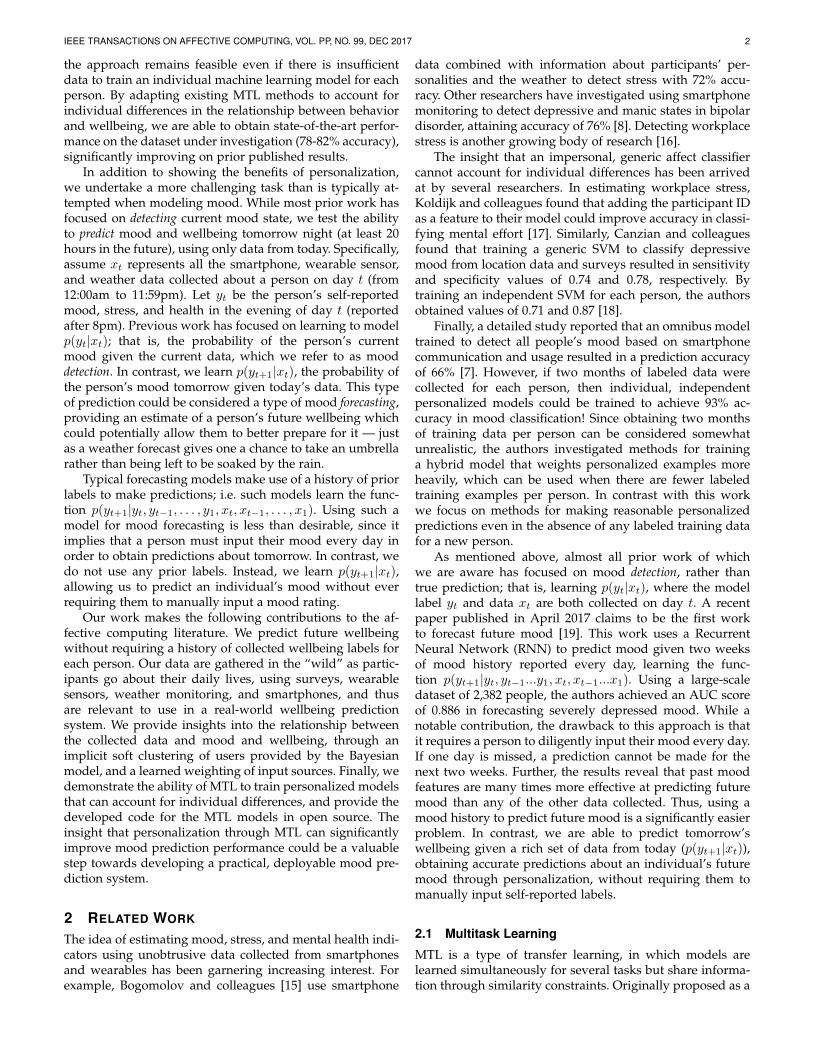
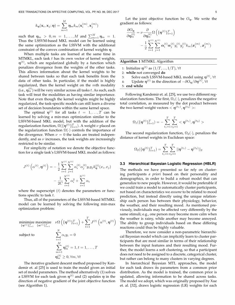
Fig. 2: Distribution of self-report labels after discarding the middle 20%. Participants are listed on the x-axis, in order oftheir average self-report value for that label (each participant is one column). Almost all participants have data from bothlabel classes.

out/calm), and health (sick/healthy) on a visual analogscale from 0-100; these scores are split based on the medianvalue to create binary classification labels. Previous workhas relied on discarding the most neutral scores before creat-ing binary labels in order to disambiguate the classificationproblem; i.e., the middle 40% of scores were discarded dueto their questionable nature as either a ‘happy’ or ‘sad’ state[9], [10]. We instead make the problem decidedly harder bydiscarding only the middle 20% of scores. We also discardparticipants with less than 10 days worth of data, since theycould not provide enough data to train viable models. Theresulting dataset comprises 104 users and 1842 days.

Figure 2 shows the raw values reported for mood, stress,and health for each participant after the middle 20% ofscores have been removed. Points appearing above theremoved values are assigned a positive classification la-bel, while points below are assigned a negative label. Asis apparent from the figures, although some participantspredominantly report one label class almost all participants’reports span the two classes. This implies that the needfor personalization is not simply due to the fact that someparticipants are consistently sad while some are consistentlyhappy, for example. Personalization is required becausepeople react differently to very similar stimuli, and a single,impersonal classifier cannot capture these differences.

4.2 Features

To predict the labels, 343 features are extracted from thesmartphone logs, location data, physiological sensor record-ings, and behavioral surveys obtained about participantseach day. Due to the rich, multi-scale nature of the datacollected, careful feature extraction is critically important,and has been explored in detail in previous work [9], [10].Here we provide a brief overview of the feature types.

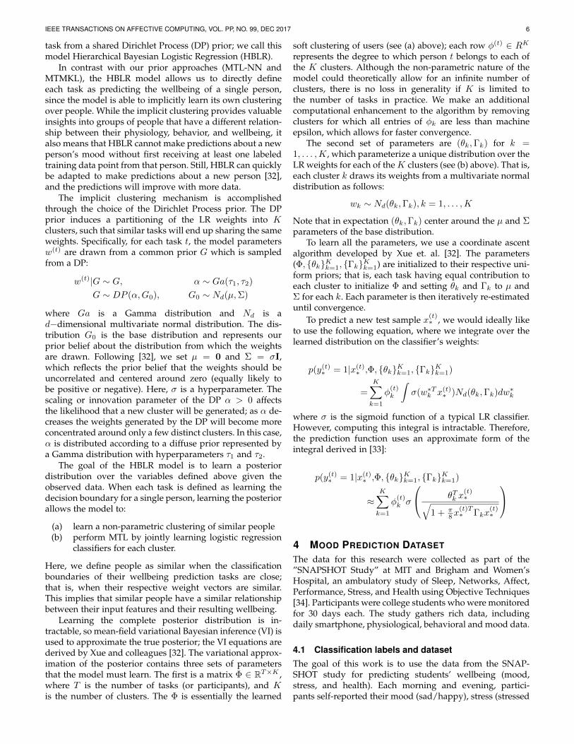
Physiology: 24-hour-a-day skin conductance (SC), skintemperature, and 3-axis acceleration were collected at 8Hz using wrist-worn Affectiva Q sensors. SC is controlledby the sympathetic nervous system (SNS); when the bodyexperiences a “fight or flight” response, a peak in the SCsignal termed an SCR will occur. Using the SC signal, weautomatically remove noise using a pre-trained algorithm[35], detect SCRs, and compute features related to theiramplitude, shape, and rate, which are shown in Figure 3.

The skin temperature and accelerometer data are also usedto compute features; from the latter, we extract measuresof activity, step count, and stillness. Since physical activityreduces stress and improves mood [36], and skin tempera-ture is related to the body’s circadian rhythm [37], we expectthese features to be highly relevant. We also weight the SCRfeatures by stillness and temperature, since we are interestedin SCRs due to emotion and stress rather than exertionor heat. In total we compute 172 physiology features overdifferent periods of the day.

Fig. 3: Features extracted for each detected, non-artifact SCR

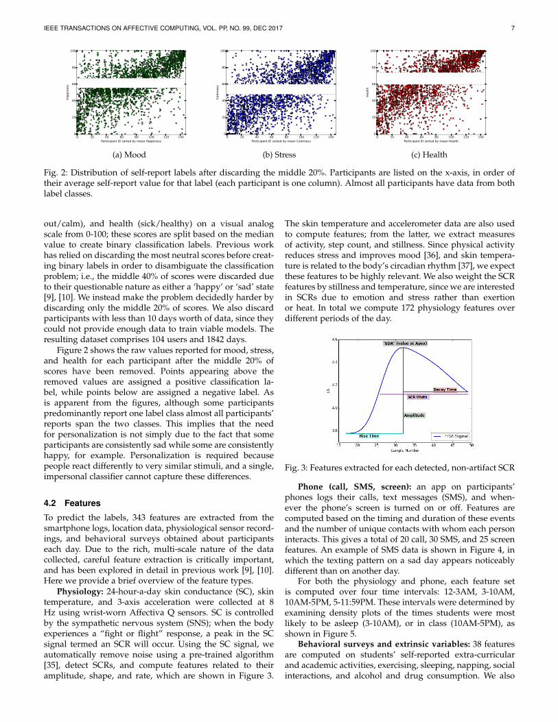
Phone (call, SMS, screen): an app on participants’phones logs their calls, text messages (SMS), and when-ever the phone’s screen is turned on or off. Features arecomputed based on the timing and duration of these eventsand the number of unique contacts with whom each personinteracts. This gives a total of 20 call, 30 SMS, and 25 screenfeatures. An example of SMS data is shown in Figure 4, inwhich the texting pattern on a sad day appears noticeablydifferent than on another day.

For both the physiology and phone, each feature setis computed over four time intervals: 12-3AM, 3-10AM,10AM-5PM, 5-11:59PM. These intervals were determined byexamining density plots of the times students were mostlikely to be asleep (3-10AM), or in class (10AM-5PM), asshown in Figure 5.

Behavioral surveys and extrinsic variables: 38 featuresare computed on students’ self-reported extra-curricularand academic activities, exercising, sleeping, napping, socialinteractions, and alcohol and drug consumption. We also

IEEE TRANSACTIONS ON AFFECTIVE COMPUTING, VOL. PP, NO. 99, DEC 2017 8

0 20 40 60 80 100Time (hours)

0

10

20

30

40

50

60

70

80

Number of SMS

Happy MoodIndifferent MoodSad Mood

Fig. 4: SMS frequency over four days

Fig. 5: Percent of participants sleeping, studying, in extra-curricular activities, and exercising throughout the day.

include 3 extrinsic variables that would be available to anysmartphone app: the participant ID, the day of the week,and whether it is a school night.

Weather: Previous studies have reported on how theweather effects mood, particularily in relation to Seasonal-Affective Disorder [37], [38]. Additionally, it is well knownthat there are particular seasons of the year (i.e. winter) thathave higher rates of poor health. Therefore, we extracted 40features about the weather from from DarkSky’s Forecast.ioAPI [39]. These features include information about sunlight,temperature, wind, Barometric pressure, and the differencebetween today’s weather and the rolling average.

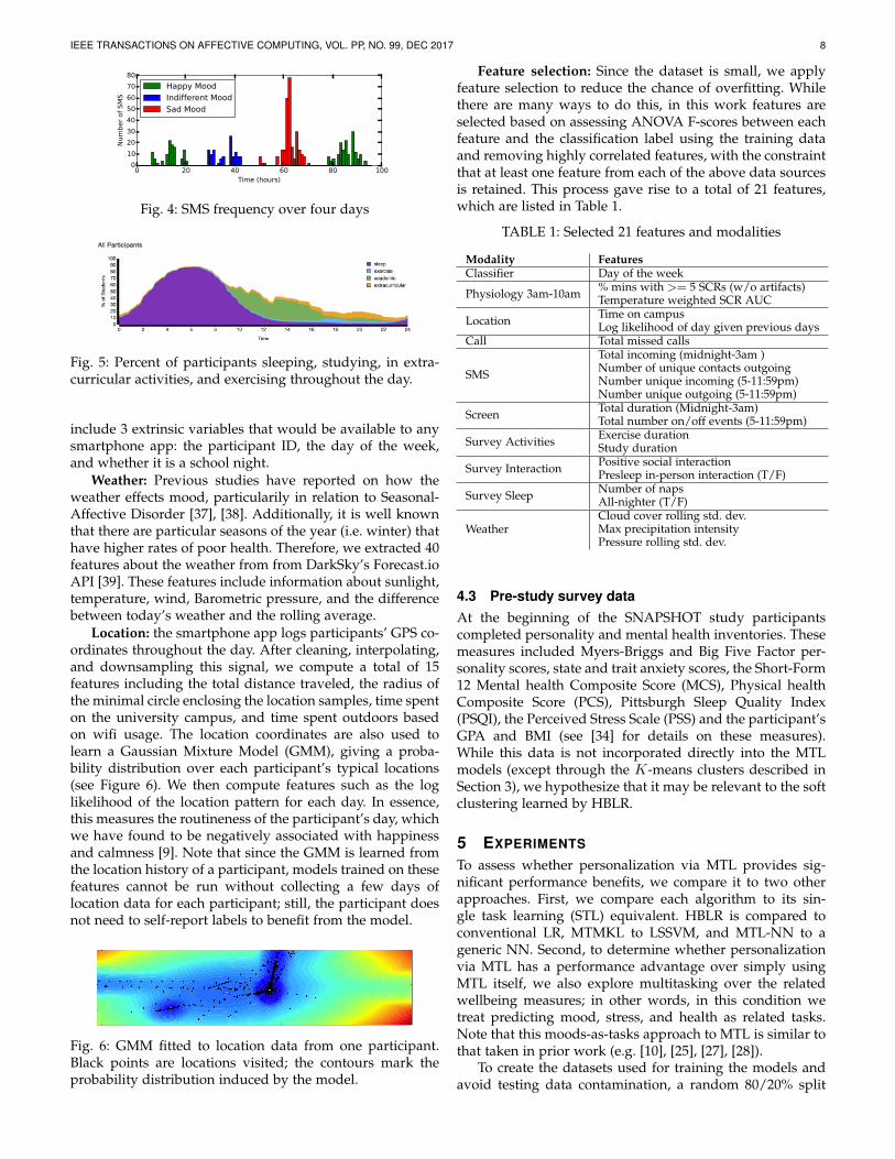
Location: the smartphone app logs participants’ GPS co-ordinates throughout the day. After cleaning, interpolating,and downsampling this signal, we compute a total of 15features including the total distance traveled, the radius ofthe minimal circle enclosing the location samples, time spenton the university campus, and time spent outdoors basedon wifi usage. The location coordinates are also used tolearn a Gaussian Mixture Model (GMM), giving a proba-bility distribution over each participant’s typical locations(see Figure 6). We then compute features such as the loglikelihood of the location pattern for each day. In essence,this measures the routineness of the participant’s day, whichwe have found to be negatively associated with happinessand calmness [9]. Note that since the GMM is learned fromthe location history of a participant, models trained on thesefeatures cannot be run without collecting a few days oflocation data for each participant; still, the participant doesnot need to self-report labels to benefit from the model.

Fig. 6: GMM fitted to location data from one participant.Black points are locations visited; the contours mark theprobability distribution induced by the model.

Feature selection: Since the dataset is small, we applyfeature selection to reduce the chance of overfitting. Whilethere are many ways to do this, in this work features areselected based on assessing ANOVA F-scores between eachfeature and the classification label using the training dataand removing highly correlated features, with the constraintthat at least one feature from each of the above data sourcesis retained. This process gave rise to a total of 21 features,which are listed in Table 1.

TABLE 1: Selected 21 features and modalities

Modality FeaturesClassifier Day of the week

Physiology 3am-10am % mins with >= 5 SCRs (w/o artifacts)Temperature weighted SCR AUC

Location Time on campusLog likelihood of day given previous days

Call Total missed calls

SMS

Total incoming (midnight-3am )Number of unique contacts outgoingNumber unique incoming (5-11:59pm)Number unique outgoing (5-11:59pm)

Screen Total duration (Midnight-3am)Total number on/off events (5-11:59pm)

Survey Activities Exercise durationStudy duration

Survey Interaction Positive social interactionPresleep in-person interaction (T/F)

Survey Sleep Number of napsAll-nighter (T/F)

WeatherCloud cover rolling std. dev.Max precipitation intensityPressure rolling std. dev.

4.3 Pre-study survey dataAt the beginning of the SNAPSHOT study participantscompleted personality and mental health inventories. Thesemeasures included Myers-Briggs and Big Five Factor per-sonality scores, state and trait anxiety scores, the Short-Form12 Mental health Composite Score (MCS), Physical healthComposite Score (PCS), Pittsburgh Sleep Quality Index(PSQI), the Perceived Stress Scale (PSS) and the participant’sGPA and BMI (see [34] for details on these measures).While this data is not incorporated directly into the MTLmodels (except through the K-means clusters described inSection 3), we hypothesize that it may be relevant to the softclustering learned by HBLR.

5 EXPERIMENTS

To assess whether personalization via MTL provides sig-nificant performance benefits, we compare it to two otherapproaches. First, we compare each algorithm to its sin-gle task learning (STL) equivalent. HBLR is compared toconventional LR, MTMKL to LSSVM, and MTL-NN to ageneric NN. Second, to determine whether personalizationvia MTL has a performance advantage over simply usingMTL itself, we also explore multitasking over the relatedwellbeing measures; in other words, in this condition wetreat predicting mood, stress, and health as related tasks.Note that this moods-as-tasks approach to MTL is similar tothat taken in prior work (e.g. [10], [25], [27], [28]).

To create the datasets used for training the models andavoid testing data contamination, a random 80/20% split

IEEE TRANSACTIONS ON AFFECTIVE COMPUTING, VOL. PP, NO. 99, DEC 2017 9

was used to partition the SNAPSHOT data into a trainand test set. We then apply 5-fold cross validation to thetraining set to test a number of different parameter settingsfor each of the algorithms described in Section 3. Finally,each model is re-trained using the optimal parameter set-tings, and tested once on the held-out testing data; the testperformance is reported in the following section.

Due to space constraints and the number of modelsinvestigated, we do not report the optimal hyperparametersettings for each model but will provide them upon request.Instead, we will simply specify that for training the NNs,we consistently used learning rate decay and the Adamoptimizer [40], and tuned the following settings: the numberand size of hidden layers, batch size, learning rate, whetheror not to apply dropout, and the L2 β weight. Based on pre-vious work that has successfully trained MTL NNs with fewsamples [22], we choose a simple, fully-connected designwith 2-4 hidden layers. For HBLR, we tuned the τ1, τ2, andσ parameters, while for MTMKL we tuned C , β, the typeof kernel (linear vs. radial basis function (RBF)), the typeof regularizer function (Ω1(·) vs Ω2(·)), and ν. For MTMKLwe also define the following modalities: classifier, location,survey interaction, survey activities, survey sleep, weather,call, physiology from 3am to 10am, screen, and SMS. Moredetail on these modalities is provided in Table 1.

All of the code for the project, which is written inPython and TensorFlow [41], has been released open-sourceand is available at https://github.com/mitmedialab/personalizedmultitasklearning

5.1 Analysis of HBLR clustersBecause the clusters learned by the HBLR model may befundamentally different than those that can be obtainedusing other methods, we are interested in defining a way toanalyze which type of participants are represented withineach cluster. For example, does a certain cluster tend tocontain participants that have a significantly higher traitanxiety score (as measured by the pre-study survey)?

The analysis is complicated by the fact there is nodiscrete assignment of participants to clusters; rather, aparticipant may have some degree of membership in manyor all of the clusters, as defined by φ(t). To solve thisissue, we first define a matrix P ∈ RT×M , where T is thenumber of participants and M is the number of pre-studymeasures (such as Big Five personality, PSS, etc.). Thus, Pt,mrepresents person t’s score on measure m. Using P, we canthen compute a score representing the average value of eachpre-study measure for each cluster, as follows:

Qk,m =

∑tPt,mφ

(t)k∑

t φ(t)k

where Q ∈ RK×M and K is the number of clusters learnedby the HBLR model. Qk,m can be considered a weightedaverage of a cluster’s pre-study trait, where the weights arethe degree of membership of each participant in that cluster.

To test whether a cluster’s Qk,m value is significantlydifferent than the group average, we use a one-samples t-test to compare Qk,m to the values for measure m reportedby participants on the pre-study survey. We apply a Bonfer-roni correction based on the number of comparisons made

across the different clusters within each outcome label (i.e.mood, stress, health).

6 RESULTS AND DISCUSSION

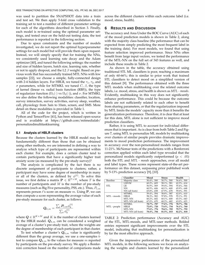
The accuracy and Area Under the ROC Curve (AUC) of eachof the mood prediction models is shown in Table 2, alongwith the majority class baseline (the peformance that can beexpected from simply predicting the most frequent label inthe training data). For most models, we found that usingfeature selection improved performance. Since NNs oftenbenefit from large input vectors, we tested the performanceof the MTL-NN on the full set of 343 features as well, andinclude these results in Table 2.

As shown in the table, the accuracy obtained usingtraditional STL ML classifiers is poor, reaching a maximumof only 60-66%; this is similar to prior work that trainedSTL classifiers to detect mood on a simplified version ofthis dataset [9]. The performance obtained with the threeMTL models when multitasking over the related outcomelabels, i.e. mood, stress, and health is shown as MTL - moods.Evidently, multitasking in this way does not significantlyenhance performance. This could be because the outcomelabels are not sufficiently related to each other to benefitfrom sharing parameters, or that the regularization imposedby MTL limits the models’ capacity more than it benefits thegeneralization performance. Therefore, it is clear that at leastfor this data, MTL alone is not sufficient to improve moodprediction classifiers.

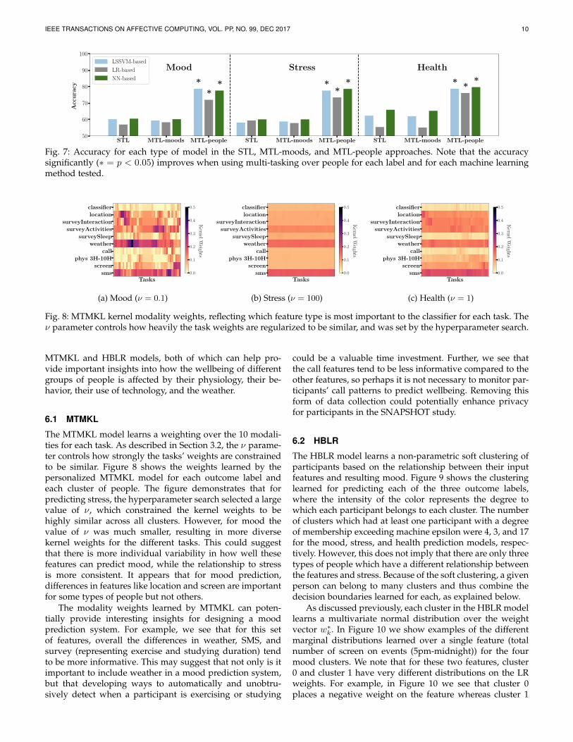
Rather, it is using MTL to account for individual differ-ences that is important. As is clear from both Table 2 and Fig-ure 7, using MTL to personalize ML models by multitaskingover clusters of similar people provides dramatic improve-ments to mood prediction performance. The improvementin accuracy over the non-personalized models ranges from11-21%. McNemar tests of the predictions with a Bonferronicorrection applied within each label type revealed that thepersonalized models significantly outperformed (p < .05)both the STL and MTL - moods approaches, over all modeland label types. These scores represent state-of-the-art per-formance on this dataset, surpassing prior published workby 5-13% prediction accuracy [9], [10].

Classifier Mood Stress HealthBaseline Majority class 50.4%, .500 50.7%, .500 54.4%, .500

STLLSSVM 60.2%, .603 58.1%, .581 62.3%, .614LR 56.9%, .569 59.4%, .594 55.4%, .544NN 60.5%, .606 60.1%, .600 65.9%, .648NN (all feats) 65.8%, .658 67.9%, .678 59.0%, .591

MTL - moodsMTMKL 59.4%, .594 58.8%, .587 62.0%, .610HBLR 58.3%, .583 57.8%, .578 55.1%, .551MTL-NN 60.2%, .602 60.1%, .600 65.3%, .643MTL-NN (all feats) 67.0%, .670 68.2%, .682 63.0%, .623

MTL - peopleMTMKL 78.7%, .787 77.6%, .776 78.7%, .786HBLR 72.0%, .720 73.4%, .734 76.1%, .760MTL-NN 77.6%, .776 78.6%, .785 79.7%, .792MTL-NN (all feats) 78.4%, .784 81.5%, .815 82.2%, .818

TABLE 2: Prediction performance (Accuracy and AUC)of the STL, MTL-moods, and MTL-user methods. Boldedentries represent significant improvements over the STLmodel, indicating that multitasking for personalization isby far the most effective approach.

Given the impressive performance of the personalizedMTL models, in the following sections we focus on analyz-ing the weights and clusters learned by the personalized

IEEE TRANSACTIONS ON AFFECTIVE COMPUTING, VOL. PP, NO. 99, DEC 2017 10

STL MTL-moods MTL-people STL MTL-moods MTL-people STL MTL-moods MTL-people50

60

70

80

90

100

Acc

urac

yMood Stress Health

**

* **

* * * *

LSSVM-basedLR-basedNN-based

Fig. 7: Accuracy for each type of model in the STL, MTL-moods, and MTL-people approaches. Note that the accuracysignificantly (∗ = p < 0.05) improves when using multi-tasking over people for each label and for each machine learningmethod tested.

Tasks

classifierlocation

surveyInteractionsurveyActivities

surveySleepweather

callphys 3H-10H

screensms 0.0

0.1

0.2

0.3

0.4

0.5

KernelW

eights

(a) Mood (ν = 0.1)

Tasks

classifierlocation

surveyInteractionsurveyActivities

surveySleepweather

callphys 3H-10H

screensms 0.0

0.1

0.2

0.3

0.4

0.5

KernelW

eights

(b) Stress (ν = 100)

Tasks

classifierlocation

surveyInteractionsurveyActivities

surveySleepweather

callphys 3H-10H

screensms 0.0

0.1

0.2

0.3

0.4

0.5

KernelW

eights

(c) Health (ν = 1)

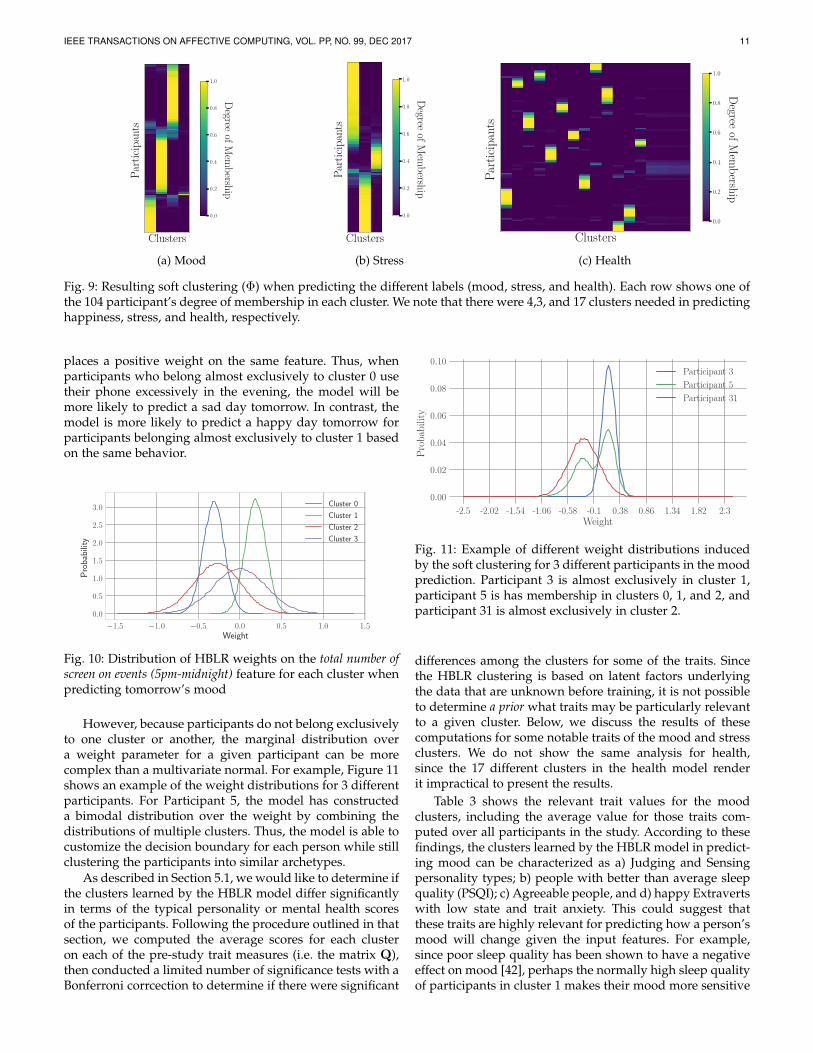
Fig. 8: MTMKL kernel modality weights, reflecting which feature type is most important to the classifier for each task. Theν parameter controls how heavily the task weights are regularized to be similar, and was set by the hyperparameter search.

MTMKL and HBLR models, both of which can help pro-vide important insights into how the wellbeing of differentgroups of people is affected by their physiology, their be-havior, their use of technology, and the weather.

6.1 MTMKL

The MTMKL model learns a weighting over the 10 modali-ties for each task. As described in Section 3.2, the ν parame-ter controls how strongly the tasks’ weights are constrainedto be similar. Figure 8 shows the weights learned by thepersonalized MTMKL model for each outcome label andeach cluster of people. The figure demonstrates that forpredicting stress, the hyperparameter search selected a largevalue of ν, which constrained the kernel weights to behighly similar across all clusters. However, for mood thevalue of ν was much smaller, resulting in more diversekernel weights for the different tasks. This could suggestthat there is more individual variability in how well thesefeatures can predict mood, while the relationship to stressis more consistent. It appears that for mood prediction,differences in features like location and screen are importantfor some types of people but not others.

The modality weights learned by MTMKL can poten-tially provide interesting insights for designing a moodprediction system. For example, we see that for this setof features, overall the differences in weather, SMS, andsurvey (representing exercise and studying duration) tendto be more informative. This may suggest that not only is itimportant to include weather in a mood prediction system,but that developing ways to automatically and unobtru-sively detect when a participant is exercising or studying

could be a valuable time investment. Further, we see thatthe call features tend to be less informative compared to theother features, so perhaps it is not necessary to monitor par-ticipants’ call patterns to predict wellbeing. Removing thisform of data collection could potentially enhance privacyfor participants in the SNAPSHOT study.

6.2 HBLR

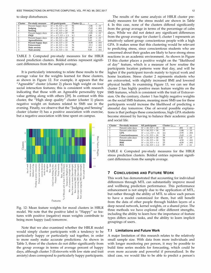
The HBLR model learns a non-parametric soft clustering ofparticipants based on the relationship between their inputfeatures and resulting mood. Figure 9 shows the clusteringlearned for predicting each of the three outcome labels,where the intensity of the color represents the degree towhich each participant belongs to each cluster. The numberof clusters which had at least one participant with a degreeof membership exceeding machine epsilon were 4, 3, and 17for the mood, stress, and health prediction models, respec-tively. However, this does not imply that there are only threetypes of people which have a different relationship betweenthe features and stress. Because of the soft clustering, a givenperson can belong to many clusters and thus combine thedecision boundaries learned for each, as explained below.

As discussed previously, each cluster in the HBLR modellearns a multivariate normal distribution over the weightvector w∗k. In Figure 10 we show examples of the differentmarginal distributions learned over a single feature (totalnumber of screen on events (5pm-midnight)) for the fourmood clusters. We note that for these two features, cluster0 and cluster 1 have very different distributions on the LRweights. For example, in Figure 10 we see that cluster 0places a negative weight on the feature whereas cluster 1

IEEE TRANSACTIONS ON AFFECTIVE COMPUTING, VOL. PP, NO. 99, DEC 2017 11

Clusters

Part

icipa

nts

0.0

0.2

0.4

0.6

0.8

1.0

Degree

ofMem

bership

(a) Mood

Clusters

Part

icipa

nts

0.0

0.2

0.4

0.6

0.8

1.0

Degree

ofMem

bership

(b) Stress

Clusters

Part

icipa

nts

0.0

0.2

0.4

0.6

0.8

1.0D

egreeofM

embership

(c) Health

Fig. 9: Resulting soft clustering (Φ) when predicting the different labels (mood, stress, and health). Each row shows one ofthe 104 participant’s degree of membership in each cluster. We note that there were 4,3, and 17 clusters needed in predictinghappiness, stress, and health, respectively.

places a positive weight on the same feature. Thus, whenparticipants who belong almost exclusively to cluster 0 usetheir phone excessively in the evening, the model will bemore likely to predict a sad day tomorrow. In contrast, themodel is more likely to predict a happy day tomorrow forparticipants belonging almost exclusively to cluster 1 basedon the same behavior.

−1.5 −1.0 −0.5 0.0 0.5 1.0 1.5Weight

0.0

0.5

1.0

1.5

2.0

2.5

3.0

Prob

abilit

y

Cluster 0Cluster 1Cluster 2Cluster 3

Fig. 10: Distribution of HBLR weights on the total number ofscreen on events (5pm-midnight) feature for each cluster whenpredicting tomorrow’s mood

However, because participants do not belong exclusivelyto one cluster or another, the marginal distribution overa weight parameter for a given participant can be morecomplex than a multivariate normal. For example, Figure 11shows an example of the weight distributions for 3 differentparticipants. For Participant 5, the model has constructeda bimodal distribution over the weight by combining thedistributions of multiple clusters. Thus, the model is able tocustomize the decision boundary for each person while stillclustering the participants into similar archetypes.

As described in Section 5.1, we would like to determine ifthe clusters learned by the HBLR model differ significantlyin terms of the typical personality or mental health scoresof the participants. Following the procedure outlined in thatsection, we computed the average scores for each clusteron each of the pre-study trait measures (i.e. the matrix Q),then conducted a limited number of significance tests with aBonferroni corrcection to determine if there were significant

-2.5 -2.02 -1.54 -1.06 -0.58 -0.1 0.38 0.86 1.34 1.82 2.3Weight

0.00

0.02

0.04

0.06

0.08

0.10

Prob

abili

ty

Participant 3Participant 5Participant 31

Fig. 11: Example of different weight distributions inducedby the soft clustering for 3 different participants in the moodprediction. Participant 3 is almost exclusively in cluster 1,participant 5 is has membership in clusters 0, 1, and 2, andparticipant 31 is almost exclusively in cluster 2.

differences among the clusters for some of the traits. Sincethe HBLR clustering is based on latent factors underlyingthe data that are unknown before training, it is not possibleto determine a prior what traits may be particularly relevantto a given cluster. Below, we discuss the results of thesecomputations for some notable traits of the mood and stressclusters. We do not show the same analysis for health,since the 17 different clusters in the health model renderit impractical to present the results.

Table 3 shows the relevant trait values for the moodclusters, including the average value for those traits com-puted over all participants in the study. According to thesefindings, the clusters learned by the HBLR model in predict-ing mood can be characterized as a) Judging and Sensingpersonality types; b) people with better than average sleepquality (PSQI); c) Agreeable people, and d) happy Extravertswith low state and trait anxiety. This could suggest thatthese traits are highly relevant for predicting how a person’smood will change given the input features. For example,since poor sleep quality has been shown to have a negativeeffect on mood [42], perhaps the normally high sleep qualityof participants in cluster 1 makes their mood more sensitive

IEEE TRANSACTIONS ON AFFECTIVE COMPUTING, VOL. PP, NO. 99, DEC 2017 12

to sleep disturbances.

Cluster Pre-study measure All participants Cluster Qk,m t p0 Percent happy days M = 49, SD = 37 56 -1.86 > .100 Judging M = 61, SD = 21 73 -7.69 < .0010 Sensing M = 47, SD = 20 57 -7.22 < .0011 Percent happy days M = 49, SD = 37 55 -1.81 > .101 PSQI M = 4.7, SD = 2.3 4.1 3.48 < .012 Percent happy days M = 49, SD = 37 41 2.29 > .102 Agreeableness M = 50, SD = 28 43 3.63 < .013 Percent happy days M = 49, SD = 37 78 -8.00 < .0013 Extraversion M = 49, SD = 30 76 -13.1 < .0013 State anxiety M = 38, SD = 10 30 10.9 < .0013 Trait anxiety M = 43, SD = 10 36 9.85 < .001

TABLE 3: Computed pre-study measures for the HBLRmood prediction clusters. Bolded entries represent signifi-cant differences from the sample average.

It is particularly interesting to relate these results to theaverage value for the weights learned for these clusters,as shown in Figure 12. For example, it appears that the“Agreeable” cluster (cluster 2) places high weight on foursocial interaction features; this is consistent with researchindicating that those with an Agreeable personality typevalue getting along with others [29]. In contrast with thiscluster, the “High sleep quality” cluster (cluster 1) placesnegative weight on features related to SMS use in theevening. Finally, we observe that the “Judging and Sensing”cluster (cluster 0) has a positive association with exercise,but a negative association with time spent on campus.

day

ofwe

ektim

eon

cam

pus

likeli

hood

ofda

yPr

eslee

pin-

perso

nint

erac

tion

Posit

iveso

ciali

nter

actio

nex

ercis

edu

ratio

nstu

dydu

ratio

nAl

l-nigh

ter

Num

.nap

sCl

oud

Cove

rRoll

ingSt

.Dev

.Pr

essu

reRo

lling

St.D

ev.

Prec

ipint

ensit

yNu

m.m

issed

calls

%of

Minu

tesw

ithat

least

5SC

Rs(3

-10a

m)

Tem

pera

ture

Weig

hted

AUC

Min.

ofsc

reen

time

(midn

ight-3

am)

Num

Scre

enon

even

ts(5

pm-m

idnigh

t)Nu

minc

oming

SMS

(midn

ight-3

am)

Num

uniqu

einc

oming

SMS

(5pm

-midn

ight)

Num

uniqu

eou

tgoin

gSM

S(5

pm-m

idnigh

t)Nu

mpe

ople

text

ed

Features

0

1

2

3

Clus

ters

−0.6

−0.4

−0.2

0.0

0.2

0.4

Mean

FeatureW

eights

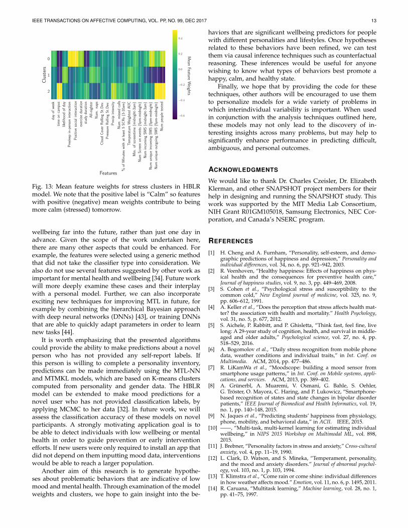
Fig. 12: Mean feature weights for mood clusters in HBLRmodel. We note that the positive label is “Happy” so fea-tures with positive (negative) mean weights contribute tobeing more happy (sad) tomorrow.

Note that we also examined whether the HBLR modelwould simply cluster participants with a tendency to beparticularly happy or particularly sad together, in orderto more easily make accurate predictions. As shown inTable 3, three of the clusters do not differ significantly fromthe group average in terms of average percent of happydays, although cluster 3 (Extroverts with low state and traitanxiety) does correspond to particularly happy participants.

The results of the same analysis of HBLR cluster pre-study measures for the stress model are shown in Table4. In this case, none of the clusters differed significantlyfrom the group average in terms of the percentage of calmdays. While we did not detect any significant differencesfrom the group average for cluster 0, cluster 1 represents anintuitively salient group: conscientious people with a highGPA. It makes sense that this clustering would be relevantto predicting stress, since conscientious students who areconcerned about their grades are likely to have strong stressreactions in an academic environment. As shown in Figure13 this cluster places a positive weight on the “likelihoodof day” feature, which is a measure of how routine theparticipants location patterns were that day, and will behigher if the participant travels mainly to typical work andhome locations. Stress cluster 2 represents students whoare extraverted, with slightly increased BMI and loweredphysical health. In examining Figure 13, we can see thatcluster 2 has highly positive mean feature weights on theSMS features, which is consistent with the trait of Extraver-sion. On the contrary, cluster 1 has highly negative weightson the social SMS features, meaning more SMS use for theseparticipants would increase the likelihood of predicting astressful day tomorrow. One of several possible explana-tions is that perhaps these conscientious, high GPA studentsbecome stressed by having to balance their academic goalsand social life.

Cluster Pre-study measure All participants Cluster Qk,m t p0 Percent calm days M = 48, SD = 38 46 .492 > .601 Percent calm days M = 48, SD = 38 55 -1.88 > .101 GPA M = 4.4, SD = .61 4.6 -3.95 < .0011 Conscientiousness M = 51, SD = 28 58 -3.43 < .012 Percent calm days M = 48, SD = 38 39 2.32 > .102 Extraversion M = 49, SD = 30 58 -4.50 < .0012 BMI M = 24, SD = 4.4 25 -4.09 < .0012 PCS M = 58, SD = 4.2 57 3.77 < .01

TABLE 4: Computed pre-study measures for the HBLRstress prediction clusters. Bolded entries represent signifi-cant differences from the sample average.

7 CONCLUSIONS AND FUTURE WORK

This work has demonstrated that accounting for individualdifferences through MTL can substantially improve moodand wellbeing prediction performance. This performanceenhancement is not simply due to the application of MTL,but rather through the ability of MTL to allow each personto have a model customized for them, but still benefitfrom the data of other people through hidden layers of adeep neural network, kernel weights, or a shared prior. Thethree methods we have explored offer different strengths,including the ability to learn how the importance of featuretypes differs across tasks, and the ability to learn implicitgroupings of users.

7.1 Limitations and Future WorkA major limitation of this research relates to the relativelysmall sample size. With data from more individuals andwith longer monitoring per person, it may be possible tobuild time series models for forecasting, which could beeven more accurate and powerful if personalized. In theideal case, we would like to be able to predict a person’s

IEEE TRANSACTIONS ON AFFECTIVE COMPUTING, VOL. PP, NO. 99, DEC 2017 13

day

ofwe

ektim

eon

cam

pus

likeli

hood

ofda

yPr

eslee

pin-

perso

nint

erac

tion

Posit

iveso

ciali

nter

actio

nex

ercis

edu

ratio

nstu

dydu

ratio

nAl

l-nigh

ter

Num

.nap

sCl

oud

Cove

rRoll

ingSt

.Dev

.Pr

essu

reRo

lling

St.D

ev.

Prec

ipint

ensit

yNu

m.m

issed

calls

%of

Minu

tesw

ithat

least

5SC

Rs(3

-10a

m)

Tem

pera

ture

Weig

hted

AUC

Min.

ofsc

reen

time

(midn

ight-3

am)

Num

Scre

enon

even

ts(5

pm-m

idnigh

t)Nu

minc

oming

SMS

(midn

ight-3

am)

Num

uniqu

einc

oming

SMS

(5pm

-midn

ight)

Num

uniqu

eou

tgoin

gSM

S(5

pm-m

idnigh

t)Nu

mpe

ople

text

ed

Features

0

1

2

Clus

ters

−0.6

−0.4

−0.2

0.0

0.2

0.4

Mean

FeatureW

eights

Fig. 13: Mean feature weights for stress clusters in HBLRmodel. We note that the positive label is “Calm” so featureswith positive (negative) mean weights contribute to beingmore calm (stressed) tomorrow.

wellbeing far into the future, rather than just one day inadvance. Given the scope of the work undertaken here,there are many other aspects that could be enhanced. Forexample, the features were selected using a generic methodthat did not take the classifier type into consideration. Wealso do not use several features suggested by other work asimportant for mental health and wellbeing [34]. Future workwill more deeply examine these cases and their interplaywith a personal model. Further, we can also incorporateexciting new techniques for improving MTL in future, forexample by combining the hierarchical Bayesian approachwith deep neural networks (DNNs) [43], or training DNNsthat are able to quickly adapt parameters in order to learnnew tasks [44].

It is worth emphasizing that the presented algorithmscould provide the ability to make predictions about a novelperson who has not provided any self-report labels. Ifthis person is willing to complete a personality inventory,predictions can be made immediately using the MTL-NNand MTMKL models, which are based on K-means clusterscomputed from personality and gender data. The HBLRmodel can be extended to make mood predictions for anovel user who has not provided classification labels, byapplying MCMC to her data [32]. In future work, we willassess the classification accuracy of these models on novelparticipants. A strongly motivating application goal is tobe able to detect individuals with low wellbeing or mentalhealth in order to guide prevention or early interventionefforts. If new users were only required to install an app thatdid not depend on them inputting mood data, interventionswould be able to reach a larger population.

Another aim of this research is to generate hypothe-ses about problematic behaviors that are indicative of lowmood and mental health. Through examination of the modelweights and clusters, we hope to gain insight into the be-

haviors that are significant wellbeing predictors for peoplewith different personalities and lifestyles. Once hypothesesrelated to these behaviors have been refined, we can testthem via causal inference techniques such as counterfactualreasoning. These inferences would be useful for anyonewishing to know what types of behaviors best promote ahappy, calm, and healthy state.

Finally, we hope that by providing the code for thesetechniques, other authors will be encouraged to use themto personalize models for a wide variety of problems inwhich interindividual variability is important. When usedin conjunction with the analysis techniques outlined here,these models may not only lead to the discovery of in-teresting insights across many problems, but may help tosignificantly enhance performance in predicting difficult,ambiguous, and personal outcomes.

ACKNOWLEDGMENTS

We would like to thank Dr. Charles Czeisler, Dr. ElizabethKlerman, and other SNAPSHOT project members for theirhelp in designing and running the SNAPSHOT study. Thiswork was supported by the MIT Media Lab Consortium,NIH Grant R01GM105018, Samsung Electronics, NEC Cor-poration, and Canada’s NSERC program.

REFERENCES

[1] H. Cheng and A. Furnham, “Personality, self-esteem, and demo-graphic predictions of happiness and depression,” Personality andindividual differences, vol. 34, no. 6, pp. 921–942, 2003.

[2] R. Veenhoven, “Healthy happiness: Effects of happiness on phys-ical health and the consequences for preventive health care,”Journal of happiness studies, vol. 9, no. 3, pp. 449–469, 2008.

[3] S. Cohen et al., “Psychological stress and susceptibility to thecommon cold,” New England journal of medicine, vol. 325, no. 9,pp. 606–612, 1991.

[4] A. Keller et al., “Does the perception that stress affects health mat-ter? the association with health and mortality.” Health Psychology,vol. 31, no. 5, p. 677, 2012.

[5] S. Aichele, P. Rabbitt, and P. Ghisletta, “Think fast, feel fine, livelong: A 29-year study of cognition, health, and survival in middle-aged and older adults,” Psychological science, vol. 27, no. 4, pp.518–529, 2016.

[6] A. Bogomolov et al., “Daily stress recognition from mobile phonedata, weather conditions and individual traits,” in Int. Conf. onMultimedia. ACM, 2014, pp. 477–486.

[7] R. LiKamWa et al., “Moodscope: building a mood sensor fromsmartphone usage patterns,” in Int. Conf. on Mobile systems, appli-cations, and services. ACM, 2013, pp. 389–402.

[8] A. Grunerbl, A. Muaremi, V. Osmani, G. Bahle, S. Oehler,G. Troster, O. Mayora, C. Haring, and P. Lukowicz, “Smartphone-based recognition of states and state changes in bipolar disorderpatients,” IEEE Journal of Biomedical and Health Informatics, vol. 19,no. 1, pp. 140–148, 2015.

[9] N. Jaques et al., “Predicting students’ happiness from physiology,phone, mobility, and behavioral data,” in ACII. IEEE, 2015.

[10] ——, “Multi-task, multi-kernel learning for estimating individualwellbeing,” in NIPS 2015 Workshop on Multimodal ML, vol. 898,2015.

[11] J. Brebner, “Personality factors in stress and anxiety,” Cross-culturalanxiety, vol. 4, pp. 11–19, 1990.

[12] L. Clark, D. Watson, and S. Mineka, “Temperament, personality,and the mood and anxiety disorders.” Journal of abnormal psychol-ogy, vol. 103, no. 1, p. 103, 1994.

[13] T. Klimstra et al., “Come rain or come shine: individual differencesin how weather affects mood.” Emotion, vol. 11, no. 6, p. 1495, 2011.

[14] R. Caruana, “Multitask learning,” Machine learning, vol. 28, no. 1,pp. 41–75, 1997.

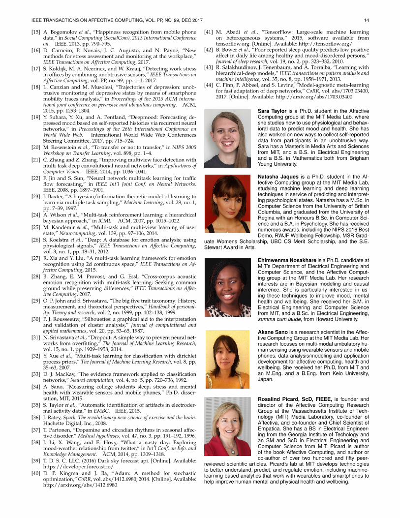
IEEE TRANSACTIONS ON AFFECTIVE COMPUTING, VOL. PP, NO. 99, DEC 2017 14

[15] A. Bogomolov et al., “Happiness recognition from mobile phonedata,” in Social Computing (SocialCom), 2013 International Conferenceon. IEEE, 2013, pp. 790–795.

[16] D. Carneiro, P. Novais, J. C. Augusto, and N. Payne, “Newmethods for stress assessment and monitoring at the workplace,”IEEE Transactions on Affective Computing, 2017.

[17] S. Koldijk, M. A. Neerincx, and W. Kraaij, “Detecting work stressin offices by combining unobtrusive sensors,” IEEE Transactions onAffective Computing, vol. PP, no. 99, pp. 1–1, 2017.

[18] L. Canzian and M. Musolesi, “Trajectories of depression: unob-trusive monitoring of depressive states by means of smartphonemobility traces analysis,” in Proceedings of the 2015 ACM interna-tional joint conference on pervasive and ubiquitous computing. ACM,2015, pp. 1293–1304.

[19] Y. Suhara, Y. Xu, and A. Pentland, “Deepmood: Forecasting de-pressed mood based on self-reported histories via recurrent neuralnetworks,” in Proceedings of the 26th International Conference onWorld Wide Web. International World Wide Web ConferencesSteering Committee, 2017, pp. 715–724.

[20] M. Rosenstein et al., “To transfer or not to transfer,” in NIPS 2005Workshop on Transfer Learning, vol. 898, pp. 1–4.

[21] C. Zhang and Z. Zhang, “Improving multiview face detection withmulti-task deep convolutional neural networks,” in Applications ofComputer Vision. IEEE, 2014, pp. 1036–1041.

[22] F. Jin and S. Sun, “Neural network multitask learning for trafficflow forecasting,” in IEEE Int’l Joint Conf. on Neural Networks.IEEE, 2008, pp. 1897–1901.

[23] J. Baxter, “A bayesian/information theoretic model of learning tolearn via multiple task sampling,” Machine Learning, vol. 28, no. 1,pp. 7–39, 1997.

[24] A. Wilson et al., “Multi-task reinforcement learning: a hierarchicalbayesian approach,” in ICML. ACM, 2007, pp. 1015–1022.

[25] M. Kandemir et al., “Multi-task and multi-view learning of userstate,” Neurocomputing, vol. 139, pp. 97–106, 2014.

[26] S. Koelstra et al., “Deap: A database for emotion analysis; usingphysiological signals,” IEEE Transactions on Affective Computing,vol. 3, no. 1, pp. 18–31, 2012.

[27] R. Xia and Y. Liu, “A multi-task learning framework for emotionrecognition using 2d continuous space,” IEEE Transactions on Af-fective Computing, 2015.

[28] B. Zhang, E. M. Provost, and G. Essl, “Cross-corpus acousticemotion recognition with multi-task learning: Seeking commonground while preserving differences,” IEEE Transactions on Affec-tive Computing, 2017.

[29] O. P. John and S. Srivastava, “The big five trait taxonomy: History,measurement, and theoretical perspectives,” Handbook of personal-ity: Theory and research, vol. 2, no. 1999, pp. 102–138, 1999.

[30] P. J. Rousseeuw, “Silhouettes: a graphical aid to the interpretationand validation of cluster analysis,” Journal of computational andapplied mathematics, vol. 20, pp. 53–65, 1987.

[31] N. Srivastava et al., “Dropout: A simple way to prevent neural net-works from overfitting,” The Journal of Machine Learning Research,vol. 15, no. 1, pp. 1929–1958, 2014.

[32] Y. Xue et al., “Multi-task learning for classification with dirichletprocess priors,” The Journal of Machine Learning Research, vol. 8, pp.35–63, 2007.

[33] D. J. MacKay, “The evidence framework applied to classificationnetworks,” Neural computation, vol. 4, no. 5, pp. 720–736, 1992.

[34] A. Sano, “Measuring college students sleep, stress and mentalhealth with wearable sensors and mobile phones,” Ph.D. disser-tation, MIT, 2015.

[35] S. Taylor et al., “Automatic identification of artifacts in electroder-mal activity data,” in EMBC. IEEE, 2015.

[36] J. Ratey, Spark: The revolutionary new science of exercise and the brain.Hachette Digital, Inc., 2008.

[37] T. Partonen, “Dopamine and circadian rhythms in seasonal affec-tive disorder,” Medical hypotheses, vol. 47, no. 3, pp. 191–192, 1996.

[38] J. Li, X. Wang, and E. Hovy, “What a nasty day: Exploringmood-weather relationship from twitter,” in Int’l Conf. on Info. andKnowledge Management. ACM, 2014, pp. 1309–1318.

[39] T. D. S. C. LLC. (2016) Dark sky forecast api. [Online]. Available:https://developer.forecast.io/

[40] D. P. Kingma and J. Ba, “Adam: A method for stochasticoptimization,” CoRR, vol. abs/1412.6980, 2014. [Online]. Available:http://arxiv.org/abs/1412.6980

[41] M. Abadi et al., “TensorFlow: Large-scale machine learningon heterogeneous systems,” 2015, software available fromtensorflow.org. [Online]. Available: http://tensorflow.org/

[42] B. Bower et al., “Poor reported sleep quality predicts low positiveaffect in daily life among healthy and mood-disordered persons,”Journal of sleep research, vol. 19, no. 2, pp. 323–332, 2010.

[43] R. Salakhutdinov, J. Tenenbaum, and A. Torralba, “Learning withhierarchical-deep models,” IEEE transactions on pattern analysis andmachine intelligence, vol. 35, no. 8, pp. 1958–1971, 2013.

[44] C. Finn, P. Abbeel, and S. Levine, “Model-agnostic meta-learningfor fast adaptation of deep networks,” CoRR, vol. abs/1703.03400,2017. [Online]. Available: http://arxiv.org/abs/1703.03400

Sara Taylor is a Ph.D. student in the AffectiveComputing group at the MIT Media Lab, whereshe studies how to use physiological and behav-ioral data to predict mood and health. She hasalso worked on new ways to collect self-reporteddata from participants in an unobtrusive way.Sara has a Master’s in Media Arts and Sciencesfrom MIT, and a B.S. in Electrical Engineeringand a B.S. in Mathematics both from BrighamYoung University.

Natasha Jaques is a Ph.D. student in the Af-fective Computing group at the MIT Media Lab,studying machine learning and deep learningtechniques in service of predicting and interpret-ing psychological states. Natasha has a M.Sc. inComputer Science from the University of BritishColumbia, and graduated from the University ofRegina with an Honours B.Sc. in Computer Sci-ence and a B.A. in Psychology. She has receivednumerous awards, including the NIPS 2016 BestDemo, RWJF Wellbeing Fellowship, MSR Grad-

uate Womens Scholarship, UBC CS Merit Scholarship, and the S.E.Stewart Award in Arts.

Ehimwenma Nosakhare is a Ph.D. candidate atMIT’s Department of Electrical Engineering andComputer Science, and the Affective Comput-ing group at the MIT Media Lab. Her researchinterests are in Bayesian modeling and causalinference. She is particularly interested in us-ing these techniques to improve mood, mentalhealth and wellbeing. She received her S.M. inElectrical Engineering and Computer Sciencefrom MIT, and a B.Sc. in Electrical Engineering,summa cum laude, from Howard University.

Akane Sano is a research scientist in the Affec-tive Computing Group at the MIT Media Lab. Herresearch focuses on multi-modal ambulatory hu-man sensing using wearable sensors and mobilephones, data analysis/modeling and applicationdevelopment for affective computing, health andwellbeing. She received her Ph.D, from MIT andan M.Eng. and a B.Eng. from Keio University,Japan.

Rosalind Picard, ScD, FIEEE, is founder anddirector of the Affective Computing ResearchGroup at the Massachusetts Institute of Tech-nology (MIT) Media Laboratory, co-founder ofAffectiva, and co-founder and Chief Scientist ofEmpatica. She has a BS in Electrical Engineer-ing from the Georgia Institute of Techology andan SM and ScD in Electrical Engineering andComputer Science from MIT. Picard is authorof the book Affective Computing, and author orco-author of over two hundred and fifty peer-

reviewed scientific articles. Picard’s lab at MIT develops technologiesto better understand, predict, and regulate emotion, including machine-learning based analytics that work with wearables and smartphones tohelp improve human mental and physical health and wellbeing.