IE551 - Chapter 5 - İstanbul Kültür Üniversitesiweb.iku.edu.tr/~rgozdemir/IE551/lecture...
22
1 IE551 - Chapter 5 Plant Layout 2 Definition: Plant layout (or more generally, “facility layout”) is the design and installation of systems of men, materials and equipment. In other words, it is the joint determination of the locations, sizes and configurations of multiple activities within a facility
-
Upload
trinhkhanh -
Category
Documents
-
view
214 -
download
0
Transcript of IE551 - Chapter 5 - İstanbul Kültür Üniversitesiweb.iku.edu.tr/~rgozdemir/IE551/lecture...

1
IE551 - Chapter 5
Plant Layout
2
Definition:
Plant layout (or more generally, “facility
layout”) is the design and installation of
systems of men, materials and equipment. In
other words, it is the joint determination of the
locations, sizes and configurations of multiple
activities within a facility

3
Machine Sequencing
� Machining centers (departments) are laid
out in such way that the total forward flows
on the line is maximized, or total backward
flows are minimized.
� Hollier developed two heuristic algorithms
that can achieve ordering of machines for
minimizing backtrack flows
4
Hollier Method 1
Step 1:Develop the “From-To” chart from part routing data. The data contained in the chart indicates numbers of
parts moves between machines (or work stations) in the cell. Moves into and out of the cell are not included in the chart.
Step 2:Determine the “From” and “To” sums for each machine. This is accomplished by summing all of the “From” trips and “To” trips for each machine.

5
Hollier Method 1
Step 3:Assign machines to the cell based on minimum “From” or “To” sums. The machine having the
smallest sum is selected. If the minimum value is a “To” sum, then the machine is placed at the beginning of the sequence. If the minimum value is a “From” sum, then the machine is placed at the end of the sequence.
6
Hollier Method 1
Tie breaker rules:� If a tie occurs between minimum “To” sums or minimum ”From” sums, then the machine with the
minimum “From/To” ratio is selected.
� If a minimum “To” sum is equal to a minimum “From” sum, then both machines are selected and placed at the beginning and end of the sequence, respectively.
� If both “To” and “From” sums are equal for aselected machine, it is passed over and the machine with the next lowest sum is selected.

7
Hollier Method 1
Step 5:Repeat steps 3 and 4 until all machines have been assigned.
Step 4:Reformat the From-To chart. After each machine has been selected, restructure the From-To chart
by eliminating the row and column corresponding to the selected machine and recalculate the “From” and “To” sums.
8
Example 5.1An analysis of 50 parts processed on four machines has been
summarized in the From-to chart of the following table.
Additional information is that 50 parts enter the machine
grouping at machine 3, 20 parts leave after processing at machine 1, 30 parts leave after machine 4. Determine a
logical machine arrangement using Hollier method 1.
To: 1 2 3 4
From: 1 0 5 0 25
2 30 0 0 15
3 10 40 0 0
4 10 0 0 0

9
Example 5.1 (solution)
Iteration No.1
To: 1 2 3 4 “From” Sums
From: 1 0 5 0 25 30
2 30 0 0 15 45
3 10 40 0 0 50
4 10 0 0 0 10
“To” Sums 50 45 0* 40 135
* The minimum sum value is the “To” sum for machine 3.
3Machine sequence:
10
Example 5.1 (solution)
Iteration No.2
To: 1 2 4 “From” Sums
From: 1 0 5 25 30
2 30 0 15 45
4 10 0 0 10
“To” Sums 40 5* 40 85
* The minimum sum value is the “To” sum for machine 2.
3 2Machine sequence:
11
Example 5.1 (solution)
Iteration No.3
To: 1 4 “From” Sums
From: 1 0 25 25
4 10 0 10*
“To” Sums 10* 25 35
* There are two minimum sum values in this chart.
The minimum “To” sum value for machine 1 is equal to the minimum “From” sum value for machine 4.
3 2 1 4Machine sequence:
12
Flow diagram
3 2 1 450 in40
10
30
15
25
5 10
30 out
20 out

13
Percentage of in-sequence moves
(%) which is computed by adding all of the values representing
in-sequence moves and dividing by the total number of moves
3 2 1 450 in40
10
30
15
25
5 10
30 out
20 outNumber of in-sequence moves = 40 + 30 + 25 = 95
Total number of moves = 95 + 15 + 10 + 10 + 5 = 135
Percentage of in-sequence moves = 95/135 = 0.704 = 70.4%
14
Percentage of backtracking moves
(%) which is computed by adding all of the values representing
backtracking moves and dividing by the total number of moves
3 2 1 450 in40
10
30
15
25
5 10
30 out
20 outNumber of backtracking moves = 10 + 5 = 15
Total number of moves = 95 + 15 + 10 + 10 + 5 = 135
Percentage of backtracking moves = 15/135 = 0.704 = 11.1%

15
Activity relationship analysis
� A number of factors other than material
handling cost might be of primary concern
in layout design
� Activity relationship chart (REL chart)
should be constructed in order to realize
the closeness rating between departments
16
An example of REL chart
Absolutely necessary
Especially important
Important
Ordinary closeness
Unimportant
A =
E =
I =
O =
U =
UndesirableX =

17
Proportion of each rating
A & X
RatingProportion to
the whole relations
≤≤≤≤ 5%
E ≤≤≤≤ 10%
I ≤≤≤≤ 15%
O ≤≤≤≤ 20%
U ≥≥≥≥ 50%Hence,
18
Relationship diagram
� Constitutes the 3rd step of SLP. It
converts the information in the REL chart
into a diagram
� REL diagram can either be constructed
manually or by using computer algorithms
19
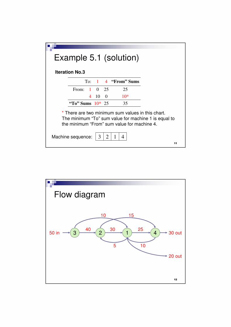
Relationship Diagramming Process (RDP)
RDP is a construction algorithm, which adds departments to the layout one by one until all departments have been placed.
Stage 1: Involves 5 steps to determine the order of placement
Step 1 � the numerical values are assigned to the closeness rating as:A= 10 000, E= 1000, I= 100, O= 10, U= 0, X= – 10 000
20
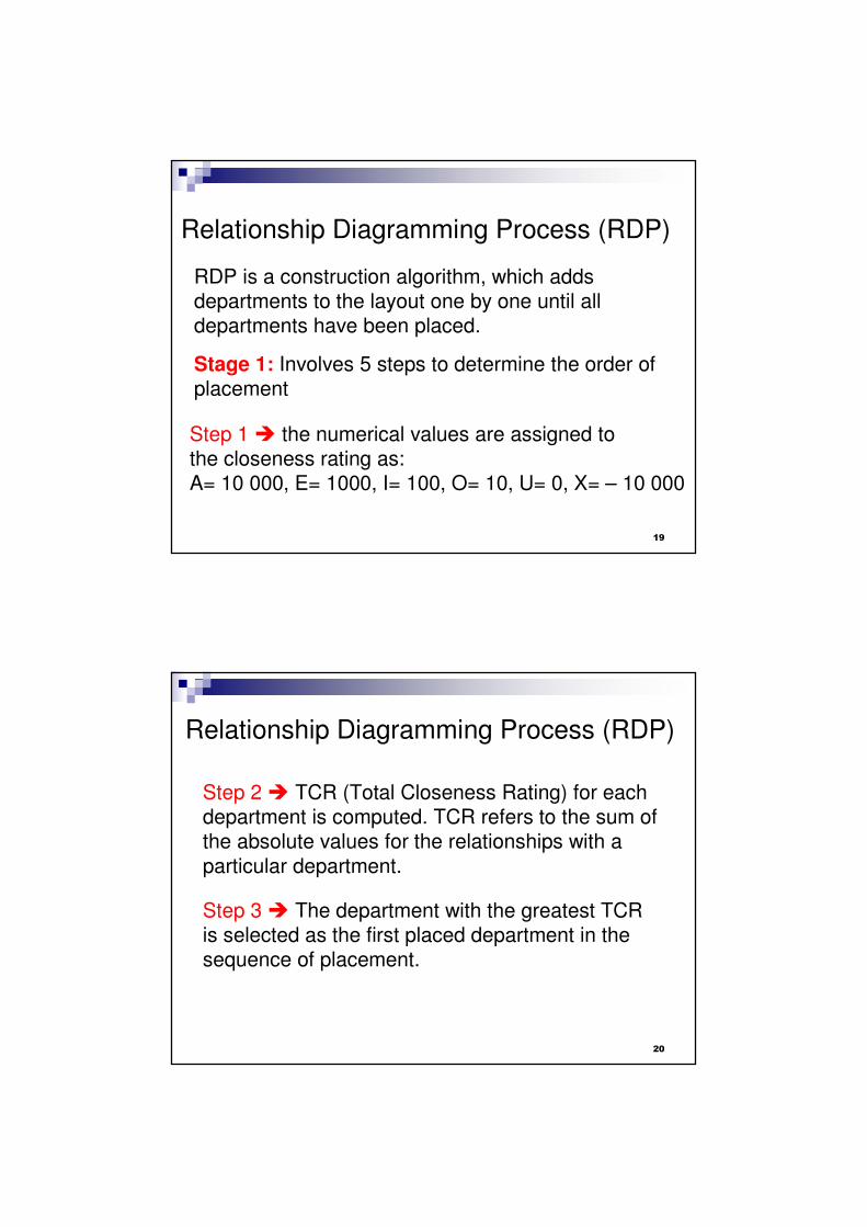
Relationship Diagramming Process (RDP)
Step 2 � TCR (Total Closeness Rating) for each department is computed. TCR refers to the sum of the absolute values for the relationships with a
particular department.
Step 3 � The department with the greatest TCR is selected as the first placed department in the sequence of placement.

21
Relationship Diagramming Process (RDP)
Step 4 � Next department in the sequence of placement is determined to satisfy the highest closeness rating with the placed department(s).
With respect to the closeness priorities A>E>I>O>U
Step 5 � Departments having X relationship with the placed department(s) are labeled as the last placed department.
Note: If ties exist during this process, TCR values are utilized to break the ties arbitrarily.
22
Relationship Diagramming Process (RDP)
Stage 2: Involves 3 steps to determine the relative locations of the departments
Step 6 � Calculate Weighted Placement Value (WPV) of locations to which the next department in the order will be assigned. WPV refers to the sum of
the numerical values for all pairs of adjacent department(s). When a location is fully adjacent, its weight equals to 1.0, and when it is partially adjacent its weight equals to 0.5.

23
Relationship Diagramming Process (RDP)
Step 8 � Assign the next department to the location with the largest WPV.
Note: If ties exist during this process, first location with the largest WPV is selected.
Step 7 � Evaluate all possible locations in counter clock-wise order, starting at the western edge of the partial layout.
24
Example 5.2
Given the activity relationship diagram (REL) determine the layout of departments using RDP.
25
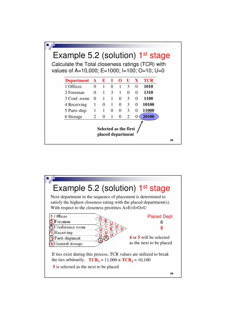
Example 5.2 (solution) 1st stage
Selected as the first
placed department
Department A E I O U X TCR
1 Offices 0 1 0 1 3 0 1010
2 Foreman 0 1 3 1 0 0 1310
3 Conf. room 0 1 1 0 3 0 1100
4 Receiving 1 0 1 0 3 0 10100
5 Parts ship. 1 1 0 0 3 0 11000
6 Storage 2 0 1 0 2 0 20100
Calculate the Total closeness ratings (TCR) with values of A=10,000; E=1000; I=100; O=10; U=0
26
Example 5.2 (solution) 1st stageNext department in the sequence of placement is determined to
satisfy the highest closeness rating with the placed department(s).
With respect to the closeness priorities A>E>I>O>U
Placed Dept.
6
4 or 5 will be selected
as the next to be placed
5
If ties exist during this process, TCR values are utilized to break
the ties arbitrarily. TCR5 = 11,000 > TCR4 = 10,100
5 is selected as the next to be placed

27
Example 5.2 (solution) 1st stageWith respect to the closeness priorities A>E>I>O>U
Placed Dept.
6
4 is selected as the next to be placed
54
28
Example 5.2 (solution) 1st stageWith respect to the closeness priorities A>E>I>O>U
Placed Dept.
6
2 is selected as the next to be placed
542
29
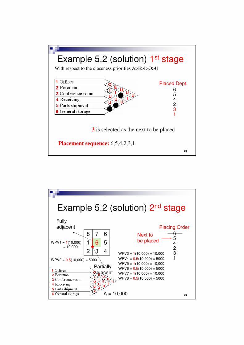
Example 5.2 (solution) 1st stageWith respect to the closeness priorities A>E>I>O>U
Placed Dept.
6
3 is selected as the next to be placed
54231
Placement sequence: 6,5,4,2,3,1
30
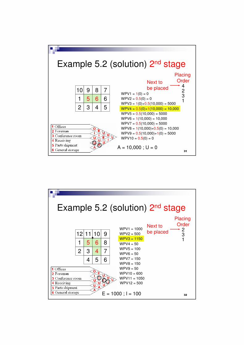
Example 5.2 (solution) 2nd stage
Placing Order
654231
61
2 3 4
5
678 Next to
be placed
A = 10,000
Fully
adjacent
WPV1 = 1(10,000)
= 10,000
WPV2 = 0.5(10,000) = 5000
Partially
adjacent
WPV3 = 1(10,000) = 10,000
WPV4 = 0.5(10,000) = 5000
WPV5 = 1(10,000) = 10,000
WPV6 = 0.5(10,000) = 5000
WPV7 = 1(10,000) = 10,000
WPV8 = 0.5(10,000) = 5000
31
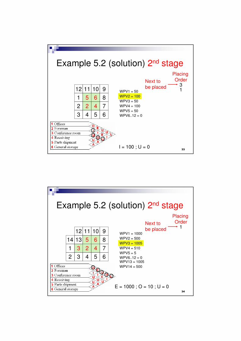
Example 5.2 (solution) 2nd stagePlacing
Order423165
3 4 5
6
789
Next to
be placed
A = 10,000 ; U = 0
WPV2 = 0.5(0) = 0
2
1
10
WPV3 = 1(0)+0.5(10,000) = 5000
WPV4 = 0.5(0)+1(10,000) = 10,000
WPV5 = 0.5(10,000) = 5000
WPV6 = 1(10,000) = 10,000
WPV7 = 0.5(10,000) = 5000
WPV8 = 1(10,000)+0.5(0) = 10,000
WPV1 = 1(0) = 0
WPV9 = 0.5(10,000)+1(0) = 5000
WPV10 = 0.5(0) = 0
32
Example 5.2 (solution) 2nd stagePlacing
Order231
65
3 4
5 6
7
8
9
Next to
be placed
E = 1000 ; I = 100
WPV2 = 500
2
1
10WPV3 = 1150
WPV4 = 50
WPV5 = 100
WPV6 = 50
WPV7 = 150
WPV8 = 150
WPV1 = 1000
WPV9 = 50
WPV10 = 600
4
11
WPV11 = 1050
12
WPV12 = 500
33
Example 5.2 (solution) 2nd stagePlacing
Order31
65
2 4
5 6
7
Next to
be placed
I = 100 ; U = 0
2
1
WPV1 = 50
WPV2 = 100
WPV3 = 50
WPV4 = 100
4
9
WPV5 = 50
10
WPV6..12 = 0
8
1112
3
34
Example 5.2 (solution) 2nd stagePlacing
Order1
65
2 4
5 6
7
Next to
be placed
E = 1000 ; O = 10 ; U = 0
3
13
WPV1 = 1000
WPV2 = 500
WPV3 = 1005
WPV4 = 510
4
9
WPV5 = 5
10
WPV6..12 = 0
8
1112
3
1
2
14
WPV13 = 1005
WPV14 = 500

35
Example 5.2 (solution) 2nd stage
65
2 43
1
Final relationship daigram of the layout
36
CRAFT-(Computerized Relative
Allocation of Facilities Technique)
� First computer-aided layout algorithm (1963)
� The input data is represented in the form of a
From-To chart, or qualitative data.
� The main objective behind CRAFT is to minimize total transportation cost:
� Improvement-type layout algorithm
fij= material flow between departments i and j
cij= unit cost to move materials between
departments i and j
dij= rectilinear distance between departments
i and j

37
Steps in CRAFT� Calculate centroid of each department and rectilinear
distance between pairs of departments centroids (stored in a distance matrix).
� Find the cost of the initial layout by multiplying the� From-To (flow) chart,
� Unit cost matrix, and
� From-To (distance) matrix
� Improve the layout by performing all-possible two or three-way exchanges� At each iteration, CRAFT selects the interchange that results in
the maximum reduction in transportation costs
� These interchanges are continued until no further reduction is possible
38
Example (Craft)
Total movement cost = (20 x 15) + (20 x 10) + (40 x 50)
+ (20 x 20) + (20 x 5) + (20 x 10) = 3200
Initial layout
39
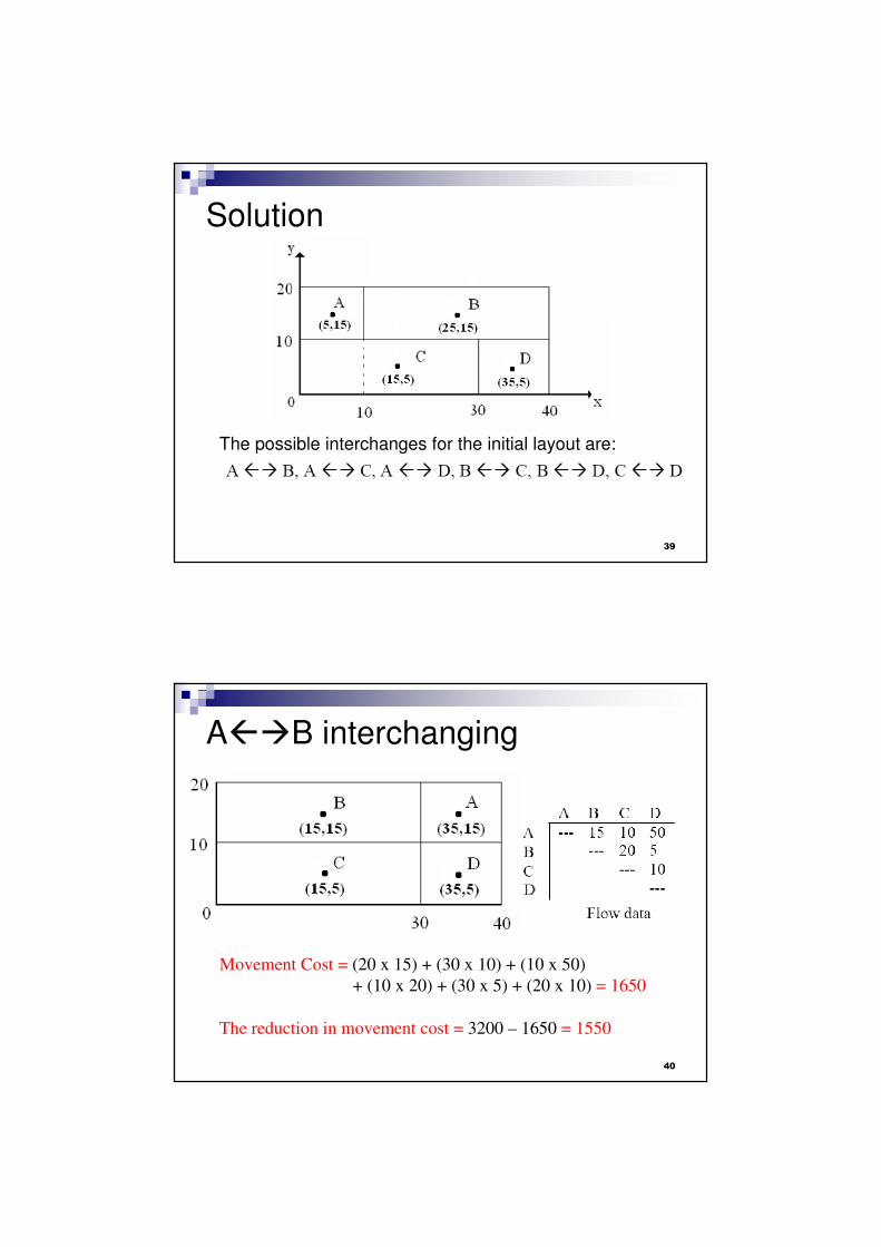
Solution
The possible interchanges for the initial layout are:
40
A��B interchanging
Movement Cost = (20 x 15) + (30 x 10) + (10 x 50)
+ (10 x 20) + (30 x 5) + (20 x 10) = 1650
The reduction in movement cost = 3200 – 1650 = 1550

41
A��C interchanging
gxC = [(100)15+(200)5]/300 = 8.33
gyC = [(100)5+(200)10]/300 = 8.33
Movement Cost = (10 x 15) + (20 x 10) + (10 x 50)
+ (23.34 x 20) + (20 x 5) + (30 x 10) = 1716.8
The reduction in movement cost = 3200 – 1716.8 = 1483.2
42
Other interchanges and savings
A��D B��C
B��D C��D
Savings: 0 Savings: 0
Savings: 1383.2 Savings: 1550

43
Current layout after A��B interchange
With this layout new pair wise interchanges are attempted as follows:
A �� D, B �� C, C �� D
�A �� B not considered since it will result no savings
�A �� C not considered since they don’t have common borders
�B �� D not considered since they don’t have common borders
44
Interchanges and savings
A��D B��CSavings: 0 Savings: 0
C��D Savings: 0
So, the current layout is the best
layout that CRAFT can find