IE 305-Part 2 Stephen B. Vardeman - Iowa State...

Engineering Economy OutlineIE 305-Part 2

Stephen B. Vardeman

ISU

Fall 2013

Stephen B. Vardeman (ISU) Engineering Economy Outline Fall 2013 1 / 52

Kinds of Production Costs

Costs incurred in production can be classified in many helpful ways.

Manufacturing costs include direct raw material and labor costs andmanufacturing overhead (like machine maintenance costs).

Manufacturing costs of materials include those of raw materialsawaiting use, those in process, and those in finished inventory awaitingsale and delivery.

Non-manufacturing costs include general company overhead, salescosts, and administrative costs.

Costs incurred generating particular revenue are recognized as expenses inthe period that the revenue is recognized.

Period costs are matched on a time period basis (and are usuallynon-manufacturing costs).

Product costs are matched on the basis of output produced (and areoften manufacturing costs).


Costs and Production Volume

Amount of production accomplished is quantified in terms of a volumeindex, like number of parts or assembled units or gallons of output. Howdifferent costs vary according to the value of such an index is important.Fixed costs are those associated with maintaining a basic operatingcapacity and don’t change with the volume index. Variable costs dependupon the level of the volume index. Some costs are mixed costs in thatthey are constant for small values of the volume index and then increaseafter some threshold level of the index is crossed.

The average unit cost for some production is just that, namely

cost of productioncorresponding value of the volume index


Formal and Informal Cost Considerations forDecision-Making

When making business decisions (choosing between opportunities) onealways considers differences in total costs between alternatives, i.e.differential costs. These are considered only going forward/in the future,i.e. ignoring sunk costs that are in the past and cannot be changed.

As one considers business (or life) opportunities, even if no formal analysisis done, account should be taken of opportunity costs. These arepotential benefits implicitly given up when one does something, becausefinite energy, time, resources then dictate that one must then fail to doother things.

A marginal cost associated with production is the cost of producing oneadditional unit of the volume index (based on a particular level of thevalue index). (This is effectively the derivative of the production-cost-versus-volume-index curve.)


Linear Production Costs

At least as an approximation to reality, it is often useful to modelproduction costs as linear in the volume index. That is, for

F = a fixed production cost

and (a constant in the volume index)

v = variable production cost per unit

for volume index, x , the production cost is

F + vx

and

average unit cost =F + vxx

= v +Fx


Profit for Linear Production Costs and Constant SellingPrice

Then ifp = selling price per unit

is fixed, i.e. doesn’t change with

x = sales volume

for Φ a profit from production

Φ = sales revenue− production cost= px − (F + vx)= −F + (p − v) x


Linear Production Costs and Constant Selling Price(continued)

The slope of the linear relationship between sales volume and profit is

p − v = the (per unit) contribution to margin(or marginal contribution).

The marginal contribution rate isp − vp

= 1− vp

The break-even volume is the value of x that produces Φ = 0, namely

xb =F

p − vthat can be expressed in dollars as

pxb =pFp − v =

F1− v

p

(the fixed cost over the marginal contribution rate).Stephen B. Vardeman (ISU) Engineering Economy Outline Fall 2013 7 / 52

Linear Production Costs and Constant Selling Price(continued)

Various problems can be set based on the basic linear relationship betweensales volume and profit

Φ = −F + (p − v) x

The equation has five entries and one can give any four and solve for thefifth. And one can contemplate the effects on profit of changing any ofthe values F , p, v , and x . In this regard, if one likes large profit, one likessmall F (one near 0 rather than being a large positive number), large x ,large p, and small v . Of course, in practice, not all of these can be variedindependently (e.g. increasing price substantially would be expected toreduce sales volume).


Depreciation Generalities

Corporate assets that wear out over time are usually subject to"depreciation." This is a calculated reduction in the value of the asset.The two main purposes of this calculation are:

1. accurate accounting for the value of assets held by a company (forboth business planning and fair representation of the state of thecompany to stockholders and others) and

2. computation of corporate income taxes—that can be reduced by usingdepreciation amounts as business expenses that offset businessincome.

In order to be subject to depreciation, assets must

1. be used in business or be held for sale,

2. have a definite useful life longer than 1 year, and

3. wear out, lose value, or become obsolete with time.



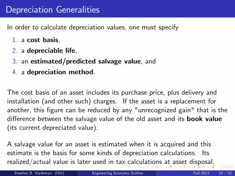
In order to calculate depreciation values, one must specify

1. a cost basis,2. a depreciable life,3. an estimated/predicted salvage value, and4. a depreciation method.

The cost basis of an asset includes its purchase price, plus delivery andinstallation (and other such) charges. If the asset is a replacement foranother, this figure can be reduced by any "unrecognized gain" that is thedifference between the salvage value of the old asset and its book value(its current depreciated value).

A salvage value for an asset is estimated when it is acquired and thisestimate is the basis for some kinds of depreciation calculations. Itsrealized/actual value is later used in tax calculations at asset disposal.



Depreciation methods consist of

1. those used for setting book values (the depreciated values) of theassets that a business owns, and

2. those used in determining corporate income taxes.

Depreciable lives are set by a firm (possibly using published governmentguidelines) for book depreciation and are specified by law for taxdepreciation. In the case of current US tax depreciation, all assets thatcan be depreciated for tax purposes fall into classes with 3-,5-,7-,10-,15-,20-,27.5-, or 39-year depreciation lives.


Book Depreciation Methods-Units of Production andStraight Line methods

In some cases an asset has a useful lifetime that can be measured in termsof units of production (or volume index). Here for a cost basis I , andestimated salvage value Sest, depreciation can be computed as

Dn = depreciation for year n

=number of service units used in year n

total number of service units in the life of the asset(I − Sest)

For I and Sest as above and a depreciable/useful life of N years, thestraight line depreciation method sets each Dn at

Dn = D ≡I − SestN


Sum of Year Digits Method

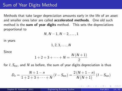
Methods that take larger depreciation amounts early in the life of an assetand smaller ones later are called accelerated methods. One old suchmethod is the sum of year digits method. This sets the depreciationsproportional to

N,N − 1,N − 2, . . . , 1

in years1, 2, 3, . . . ,N

Since

1+ 2+ 3+ · · ·+N = N (N + 1)2

for I ,Sest, and N as before, the sum of year digits depreciation is thus

Dn =N + 1− n

1+ 2+ 3+ · · ·+N (I − Sest) =2 (N + 1− n)N (N + 1)

(I − Sest)


Declining Balance Method

The most common accelerated depreciation method is a kind ofgeometrically decreasing depreciation method called the decliningbalance method. The simplest version of this ignores any predictedsalvage value Sest and uses a multiplier

0 < α ≤ 2N

For Bn the book value (balance) at the end of year n, the simple decliningbalance depreciation is

Dn = αBn−1

Simple algebra shows that under this scheme

Bn = I (1− α)n and thus Dn = α (1− α)n−1 I

The α = 2/N case is called the "200%" or "double" declining balancecase and α = 1.5/N is the "150%" declining balance case.


Declining Balance Method-Adjustments for Salvage Value

Note that the simple final declining balance book value is BN = I (1− α)N

and unless a predicted salvage value is (fortuitously) this, one ends the lifeof the asset with a (positive) book value that differs from the predictedsalvage value. So adjustments are typically made to the method toaccount for this discrepancy.

Where I (1− α)N exceeds a predicted salvage value, a commonmodification of ordinary declining balance depreciation is to switch tostraight line depreciation in the first year n where straight line depreciationof the current book value over the remaining life of the asset isadvantageous. That is, one switches at the first n for which

Bn−1 − SestN + 1− n =

I (1− α)n−1 − SestN + 1− n > αBn−1

Call this first year under straight line depreciation year nswitch.


Declining Balance Method-Adjustments for Salvage Value

That is, where I (1− α)N > Sest it is common to take depreciations

D =B(nswitch−1) − SestN + 1− nswitch

=I (1− α)(nswitch−1) − Sest

N + 1− nswitchin each of years nswitch, nswitch + 1, . . . ,N.

Where I (1− α)N < Sest, one must simply stop short of depreciating theasset beyond its predicted salvage value. This means taking only thedepreciation

Bn−1 − Sestin the year n that one first would have Bn = I (1− α)n < Sest. Call thisyear nlast. Depreciations are then Dnlast = Bnlast−1 − Sest and 0 in yearsnlast + 1, . . . ,N.


(US Federal) Tax Depreciation Methods

Depreciation is an important topic for business viability since depreciationof corporate assets can be used to offset revenue, reduce taxable income,and thereby contribute to corporate net income. It is thus important toknow something about the basic rules for tax depreciation in the US.

Assets put into service by US companies before 1981 are depreciated usingbook methods (SL, SOYD, or DB). Assets put into service 1981-1986must be depreciated using an "Accelerated Cost Recovery System"specified in tax law. Assets placed in service after 1986 are treated usinga Modified Accelerated Cost Recovery System (MACRS) specified intax law. The basics of this last system/set of rules bear presentation inthe next few slides. They are based on application of book methodprinciples in a way intended to make corporate investment attractive byallowing much of an asset’s depreciation to be taken early in its life.


MACRS-Property Classes

All corporate assets depreciable under the MACRS are placed (byregulation) into 3-,5-,7-,10-,15-, or 20-year classes for "personal"properties (assets that are not real estate) and 27.5- or 39-year classes for"real" (real estate/land and buildings) properties.

MACRS depreciation on 3-,5-,7-, 10-, 15- and 20-year (personal)properties is computed using

1. a special "half year" convention that treats properties as if they wereacquired half way through a first year of ownership and used up3,5,7,10 or 15 years later (in year 4,6,8,11, or 16 of ownership) andthus spreads depreciation over one more year than the ownership classnumber,

2. the 200% declining balance method switching to the straight linemethod (when it first provides a larger depreciation) for 3-,5-,7-, and10-year properties, and

3. the 150% declining balance method switching to the straight linemethod for 15- and 20-year properties.


MACRS Table for "Personal" Properties

Here is the IRS table specifying percent of cost basis that can be taken asdepreciation for 3- through 20-year personal properties.

Figure: From IRS Publication 946


MACRS for Real Properties and Depletion

The MACRS rules for depreciating the buildings part (NOT THE LANDPART) of a depreciable real estate asset include

1. a special "half month" convention that treats properties as if theywere acquired half way through a first month of ownership and usedup 27.5 years (for residential properties) or 39 years (for commercialproperties) later and thus spreads depreciation over one more yearthan the ownership class number,

2. straight line depreciation over 27.5× 12 = 300 months for residentialreal properties, and

3. straight line depreciation over 39× 12 = 468 months for commercialreal properties.

Another topic discussed in the text’s Ch9 is depletion. This is thephysical reduction of an initial supply of natural resources (like minerals ortimber). The tax rules for subtracting the effects of depletion fromrevenue are different from depreciation rules.


Corporate Income Tax

Companies in the US are taxed on

taxable income = gross income − expenses

(where expenses include cost of goods sold, depreciation, and operatingexpenses) producing

net income = taxable income − taxes

Taxable income is taxed (as for persons) more or less "progressively," withthe "last" dollars earned in a year usually taxed at a higher rate than the"first" ones. Marginal tax rates refer to rates applied to the last dollars.An effective (or average) tax rate is

total taxtaxable income


US Corporate Tax Rates

Here is the IRS table for 2012 corporate taxes

Figure: From IRS Publication 542


Disposal of an MACRS Asset-Final Book Value, Gain orLoss

The first matter to be considered in the tax implications of disposal of anMACRS asset is the asset’s final book value. If disposal occurs after theend of the depreciation period, this is 0. If disposal occurs before the endof the depreciation period, only a half year depreciation is subtracted fromthe previous book value to arrive at the book value (in the final year ofdepreciation, this brings the book value to 0).

After finding a book value for the disposal year, there is the matter of thetax implications of a gain or loss on the property. By virtue of depreciation

final book value < cost basis

and we consider in turn the possibilities of where the actual salvage value(proceeds from sale minus selling and removal expenses, call it Sact) lies incomparison to the last book value and original cost basis. There istypically an associated gain or loss.


Disposal of an MACRS Asset-S Less Than Book Value

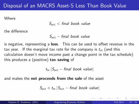
WhereSact < final book value

the differenceSact − final book value

is negative, representing a loss. This can be used to offset revenue in thetax year. If the marginal tax rate for the company is tm (and thiscalculation doesn’t move income past a change point in the tax schedule)this produces a (positive) tax saving of

tm |Sact − final book value|

and makes the net proceeds from the sale of the asset

Sact + tm |Sact − final book value|


Disposal of an MACRS Asset-S More Than Book Value

WhereSact > final book value

the differenceSact − final book value

is positive, representing a gain.

If additionally Sact < cost basis then all of the gain is an ordinary gain.

If additionally Sact > cost basis then

Sact − cost basis = capital gain

andcost basis − final book value = ordinary gain

Ordinary gains are also known as depreciation recapture.


Disposal of an MACRS Asset-Gains Tax

Where there are gains on the disposal of MACRS assets, there is tax topay on them. Presently, ordinary and capital gains are taxed at the samerate, as ordinary corporate income. But they must be kept separate foraccounting purposes, one reason being the fact that tax rules can bechanged at any time in the future, and capital and ordinary gains aretypically considered to be fundamentally different.

If the marginal tax rate for the company is tm (and this calculation doesn’tmove income past a change point in the tax schedule) this produces agains tax of

gains tax = ordinary gains tax + capital gains tax

= tm (ordinary gain) + tm (capital gain)

(where there may be 0 capital gain). The corresponding net proceedsfrom the sale of the asset are

Sact − gains taxStephen B. Vardeman (ISU) Engineering Economy Outline Fall 2013 26 / 52

Combined Federal and State Tax Rate

If

tf = federal marginal tax rate

ts = state marginal tax rate

and one computes and subtracts the (lower) state tax from income beforecomputing federal tax, it’s easy to see that with

tm = combined marginal tax rate

one hastm = tf + ts − tfts


Depreciation, Taxes, Net Income, and Cash Flows

Depreciation is not a cash flow. No money changes hands, nor areresources invested when depreciation is accounted for. But it is includedon income statements as an expense offsetting revenue and reducing taxliabilities. It thus indirectly affects project cash flows in that it reducestaxes paid, real cash outflows.

Where one wishes to determine a project cash flow from a correspondingnet income, any depreciation expense that has been subtracted fromrevenue in computing the net income should be added back in to producethe proper cash flow figure.

Cash flows are a more useful representation of project effectiveness thanproject net incomes, since the latter ignore the actual timing of cashinflows and outflows (counting costs used to produce revenues only whenthe revenues are realized) and thus also ignore the time value of money.


Tax Rate to Use for Project Analysis

When one wants to find a tax rate relevant to a potential engineeringproject, the appropriate rate is an average rate based on incrementaltaxable income and incremental tax. That is, the appropriate rate is

tax with the project − tax without the projecttaxable income with the project − taxable income without the project


Types of Project Cash Flows

Project cash flows are usually thought of as derived from the broadcategories of

1. Operating Activities (including revenues, expenses, project debtinterest, and income taxes),

2. Investing Activities (including project investments, net proceedsfrom salvage of project assets, and investments in working capital),and

3. Financing Activities (including proceeds from loans taken for theproject and repayments of principal on such loans).


Notation

In what follows, let

An = project cash flow at time n

Rn = project revenue at time n

En = project expenses1 at time n

IPn = project debt interest at time n

Tn = project income taxes at n

In = project investment at time n

Sn = project total (actual) salvage proceeds at time n

Gn = project gains tax at time n

Wn = project working capital investment at time n

Bn = proceeds from a project loan at time n

PPn = project loan principal repayments at time n1depreciation and debt interest are not included here1depreciation and debt interest are not included here1depreciation and debt interest are not included here1depreciation and debt interest are not included here1depreciation and debt interest are not included here1depreciation and debt interest are not included here1depreciation and debt interest are not included here1depreciation and debt interest are not included here


Cash Flow Development

In the notation on the previous slide

An = Rn − En − IPn − Tn (from Operating activity)− In + (Sn − Gn)−Wn (from Investment activity)+ Bn − PPn (from Financing activity)

In the event that a project does not change a corporate marginal tax ratetm, this can be rewritten as

An = (Rn − En − IPn) (1− tm) + tmDn− In + (Sn − Gn)−Wn

+ Bn − PPn

and the term tmDn is sometimes called the depreciation tax shield.


Working Capital and Loans

The "working capital" (Wn) elements of the cash flow developmentconcern funds that must be dedicated to cash, accounts receivable, andinventory to make a project work. For example, raw materials must beowned, as must work in progress and finished goods awaiting sale. This isaccounted for by negative cash flows that are matched by later positivecash flows as (years end or) the project ends and the corresponding capitalis returned to the company.

We further reiterate that project loans (Bn) are not income andrepayments of principal on them (PPn) are not expenses. They have notax consequences. But they are cash flows and have economicconsequences.


Inflation-PPI/CPI

Inflation is a second (besides interest) aspect of the time value of money.It accounts for the fact that prices for goods and services change withtime. A dollar today may not have the same purchasing power tomorrow.Inflation occurs when prices rise/purchasing power of currency declines.Deflation occurs in the (fairly rare case) when prices decline/purchasingpower of currency rises.

Governments must try to measure inflation/deflation. The USgovernment produces the Producer Price Index (PPI) that attempts to(monthly) measure industrial prices. It also produces several versions ofthe Consumer Price Index (CPI) that attempts to measure the currentprice of a "market basket" of goods and services typically purchased byurban residents/workers. Offi cial information about the current version ofthe latter can be found at: http://www.bls.gov/news.release/pdf/cpi.pdf


CPI Details

An old version of the CPI used average prices in 1967 as a base, while newversions2 of the CPI use 1982-1984 average prices as a base. These1982-1984 average prices in various categories were set to 100 (percent)and weighted according to what fraction of an average income was spenton goods or services in a given category. In subsequent years multiples of100 representing category average prices relative to the base years areweighted together to produce a CPI. So, in theory, the ratio

CPI in year n+ kCPI in year n

is the ratio of "the market basket" prices in the two years n and n+ k.

2There are versions of the CPI that intend to describe an average US urban resident(CPI-U) and an average US urban wage earner/clerical worker (CPI—W).


CPI Reweighting

A fundamental/inescapable diffi culty involved in producing any price index(certainly including the CPI) is that products and patterns of their usechange over time. (Indeed some products will pass out of existence andnew ones will be created.) So periodic reweighting of the components ofthe CPI is absolutely inevitable.

But it is a politically sensitive question how often reweighting should bedone. This is because many US government payments (like social securitybenefits) are tied to the value of the CPI, and frequent updating can beargued to ultimately exert pressure on consumer behavior towardsubstitution of cheaper alternatives in place of more expensive ones andunderstating of the real effects of inflation (and reduction in cost-of-livingadjustments to benefits). "Chained" versions of the CPIs use veryfrequent (monthly) reweighting.


Average Annual Inflation Rate

An inflation rate f such that for a good of interest

year n+ k price of the goodyear n price of the good

= (1+ f )k

is an average annual inflation rate for the good over the k yearsn, n+ 1, n+ 2, . . . , n+ k .

A rate f̄ such that

CPI in year n+ kCPI in year n

= (1+ f̄ )k

is the general (annual) inflation rate across the k yearsn, n+ 1, n+ 2, . . . , n+ k . Put differently, the general inflation rate fromyear n to year n+ k is

f̄ =(CPI in year n+ kCPI in year n

)1/k

− 1


Inflation-Actual and Constant Dollars

In the analysis of engineering projects actual dollars are just that,government-printed paper certificates that are used to pay debts. Whenwe use them in cash flow analysis, we are assuming that future inflation ordeflation will do whatever they will do to purchasing power. On the otherhand, constant dollars are estimates of future cash flows in terms of thepurchasing power of actual dollars in some base year.

For f̄ a (supposedly constant) general inflation rate, a time n cash flow in(time 0) constant dollars A′n is related to a corresponding to a time n cashflow in actual dollars, An, by

An = A′n (1+ f̄ )n

EquivalentlyA′n = An (1+ f̄ )

−n


Inflation and Economic Equivalence Calculations

There are two possibilities for doing economic equivalence calculations:

1. One may state cash flows in actual dollars and use an interest rate, i ,that is a "market" or "inflation adjusted" interest rate that iswhat one can get from a financial institution on the open market andtakes into account the combined effects of the earning value ofcapital and changes in purchasing power over time, or

2. one may state cash flows in constant dollars and use an interest rate,i ′, that is a "real" or "inflation free" interest rate that describes thetrue earning power of money with inflation/deflation effects removed.

Since taxes are paid in actual dollars, private sector economic equivalencecalculations are usually done as in 1. Since governments pay no taxes,economic equivalence analyses for long-term public projects are often doneas in 2.


Constant Dollar Economic Equivalence Analysis

To conduct a constant collar analysis one may convert cash flows An toconstant dollar cash flows A′n via

A′n = An (1+ f̄ )−n

and then consider corresponding time n = 0 net present worth under a realinterest rate i ′

A′n(1+ i ′

)−n= An

((1+ f̄ )

(1+ i ′

))−n= An

(1+ f̄ + i ′ + f̄ i ′

)−n

Note that this is completely equivalent to doing analysis with actual dollarcash flows and with market rate

i = f̄ + i ′ + f̄ i ′

computing time n = 0 net present worth.Stephen B. Vardeman (ISU) Engineering Economy Outline Fall 2013 40 / 52

Market and Real Interest Rates

The relationship between interest rates

i = f̄ + i ′ + f̄ i ′

implicit in constant dollar economic equivalence computations suggestshow a real interest rate might be computed. That is, solving the abovefor i ′ one obtains

i ′ =i − f̄1+ f̄

=1+ i1+ f̄

− 1


Effects of Inflation on Projects

Inflation has the effects on a project of

1. causing taxable income to be over-stated because depreciation is inactual dollars that are devalued in time,

2. increasing taxes because inflated actual salvage values are comparedto uninflated book values,

3. reducing real financing costs because loans are repaid in (devalued)actual dollars,

4. increasing working capital costs (a phenomenon called workingcapital drain),

5. reducing net present worth in light of 1, 2, and 4 above unlessrevenues are increased to keep pace with inflation, and

6. similarly reducing IRR unless revenues are increased to keep pacewith inflation.


Incomplete Knowledge of the Future

Measures of project economic impact like net present worth and internalrate of return are functions of all cash flows A0,A1, . . . ,AN and periodinterest rates i1, i2, . . . , iN . We have just discussed the truth that each Anis itself a function of period variables Rn,En, IPn,Dn, In,Sn,Wn,Bn,PPn,and applicable tax rates. When analysis of the probable impact of aproject is done, values of these variables are in the future, and of necessityincompletely known. One takes one’s best guess at them, but surelydoesn’t expect to get them all exactly right. The text’s Chapter 12attempts to consider means of accounting for and measuring the riskinherent in one’s incomplete knowledge of the many inputs to an NPW orIRR computation. These are break-even analysis, scenario analysis,sensitivity analysis, and probabilistic analysis.


Break-Even Analysis and Scenario Analysis

We will henceforth call a set of best guesses at the inputs to a NPWcomputation a base case of inputs. If one then picks one of the manyinputs for analysis, call it x for the time being, it’s possible to treat NPWas a function of that single input alone (by holding the rest of the inputsat their base values). A break-even point for x is a value xb that (at thebase values of the other inputs) makes NPW = 0. Typically, NPW isnegative to one side of xb and positive to the other. One exactly breakseven at x = xb.

In addition to a base case of inputs one might also specify a best case(consisting of inputs presumably most favorable to NPW) and a worstcase (consisting of inputs presumably least favorable to NPW).Comparing the corresponding NPWs (or IRRs) for the base, best andworse scenarios gives some understanding of the extremes of what valuethe project could ultimately produce.


Sensitivity Analysis

For every input to a NPW (or IRR) computation, x with base value xbase,one might compute (say)

.9xbase, .95xbase, xbase, 1.05xbase, 1.1xbase

and corresponding values of NPW (or IRR) for these values of x with theother inputs held at their base values. Then plotting points(.9,NPW.90xbase) , (.95,NPW.95xbase) , (1,NPWxbase) , (1.05,NPW1.05xbase) ,(1.1,NPW1.10xbase) one might consider the slope at 1 of the "curve" theydefine, and compare slopes across the various inputs. Large (positive ornegative) slope of a plot at 1 indicates that NPW (or IRR) is relativelysensitive to (percent) changes in the corresponding input variable. Nearlyhorizontal plots identify inputs that (at least near the base case) don’tmuch change NPW (or IRR).


Probabilistic Analysis-Distributions for Inputs

A different approach to the analysis of uncertainty in NPW (or IRR)associated with incomplete knowledge of its inputs is through providing aprobability distribution for the set of the inputs. That is, letting inputsstand for the whole set of quantities needed to produce NPW (or IRR), ifone treats inputs as random, then

NPW (inputs)

is a random variable. A (joint) distribution for inputs produces adistribution for NPW.

Convenient joint distributions for inputs treat individual inputs asindependent with means equal to respective base values. The levels ofuncertainty in the inputs can be reflected in magnitudes of standarddeviations of the inputs (used in the joint distribution). But how to gofrom this kind (or any kind) of distribution for inputs to the implieddistribution for NPW (inputs) is a separate question.


Probabilistic Analysis-Simulations

The most practical method of finding (at least approximately) thedistribution of NPW (inputs) is through simulation of a large number ofrealizations of the whole set of inputs, say

inputs1, inputs2, . . . , inputsK

and direct computation of the corresponding realizations of NPW (or IRR)

NPW (inputs1) ,NPW (inputs2) , . . . ,NPW (inputsK )

Properties of this set of simulated NPW values serve as approximations forthe theoretical properties of the random variable NPW (inputs). Arelative frequency distribution of the generated values approximates theprobability distribution of the random variable, the sample meanapproximates ENPW (inputs), and the sample variance approximatesVarNPW (inputs).


Probabilistic Analysis-Analytical Methods, Mean andVariance

The text has some very artificial/simplified/unrealistic examples of usingpencil-and-paper theoretical derivations of a probability distribution forNPW (inputs) and the mean and variance for this variable where only oneor two of its inputs are treated as random.

What is perhaps more important for IE 305 purposes is to simply recallhow to get the mean and variance for a discrete random variable from itsdistribution and to apply those ideas to problems where a distribution forNPW is been given. If the random variable NPW has possible valuesnpw1, npw2, . . . , npwM with corresponding probabilities p1, p2, . . . , pM thenthe mean and variance of the random variable are respectively

ENPW =M

∑i=1npwipi and VarNPW =

M

∑i=1(npwi − ENPW )2 pi


Probabilistic Analysis-Comparison of Projects

When comparing projects under uncertainty, one generally prefers projectswith large ENPW . But relatively small VarNPW is also typicallydesirable, in that small variance can be taken as relative certaintyregarding the economic consequence of a project. So small differencesbetween mean NPWs (or IRRs) can be unimportant if projects have wildlydifferent standard deviations of NPW (and thus varied uncertaintiesregarding the benefits of the projects).

If one has available the sets of possible values of NPW and correspondingprobabilities for two potential projects, another way to compare them is totreat NPWA and NPWB as independent random variables and find

P [NPWA ≥ NPWB ]

If this is bigger than .5, Project A might be preferable to Project B (butagain, common sense must prevail ... if Project A has a small butimportant probability of disaster, this criterion may not be a decisive one).


IE 305-Part 2 Stephen B. Vardeman - Iowa State...

Documents

Transcript of IE 305-Part 2 Stephen B. Vardeman - Iowa State...