17.4.2013

1

LECTURE N° 10- Design and Analysis Tools-

2

Lecture contributions

Coordinator of the lecture:• Karel Kabele, Faculty of Civil Engineering, CTU in Prague,

kabele@fsv.cvut.cz , http://tzb.fsv.cvut.cz/

Contributors:• Karel Kabele, Faculty of Civil Engineering, CTU in Prague,

kabele@fsv.cvut.cz , http://tzb.fsv.cvut.cz/• Pavla Dvořáková, Faculty of Civil Engineering, CTU in Prague,

pavla.dvorakova@fsv.cvut.cz, http://tzb.fsv.cvut.cz/

IDES-E

DU

17.4.2013

2

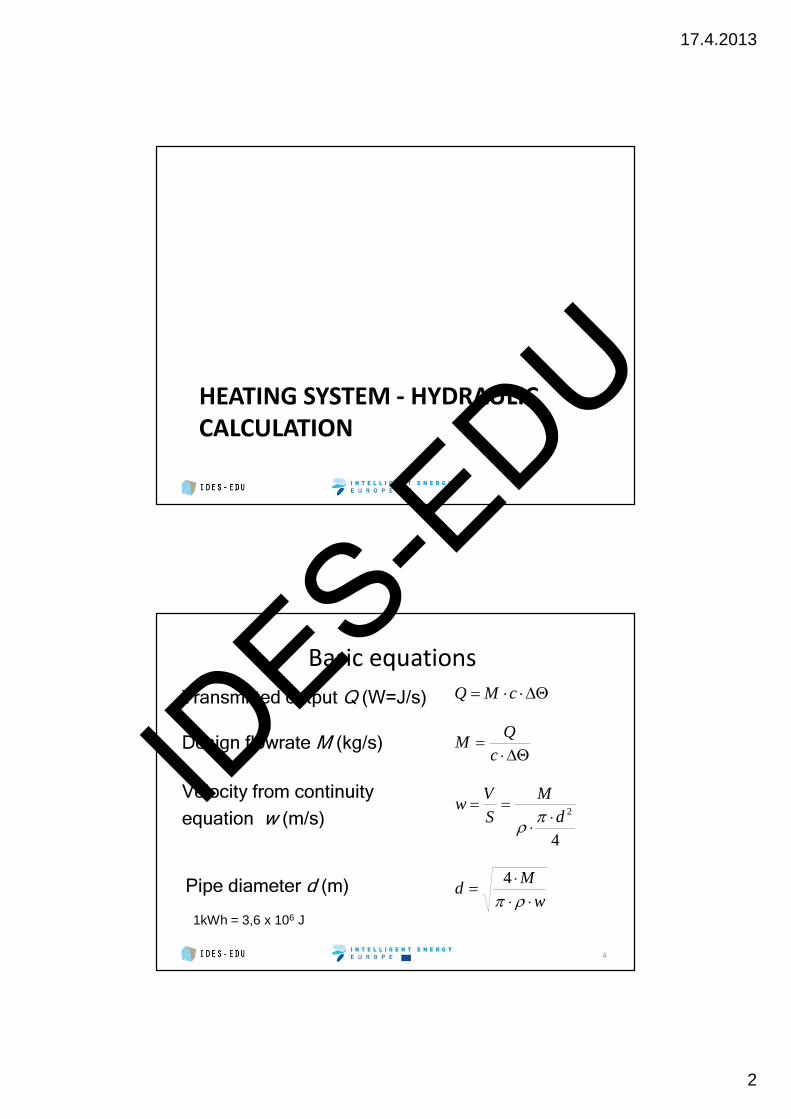
HEATING SYSTEM - HYDRAULICCALCULATION

Basic equationsTransmitted output Q (W=J/s) Q M c t= ⋅ ⋅∆

1kWh = 3,6 x 106 J

Design flowrate M (kg/s)

Pipe diameter d (m)

4

∆Θ⋅⋅= cMQ

∆Θ⋅=

c

QM

4

2dM

S

Vw

⋅⋅

==πρ

w

Md

⋅⋅

⋅=

ρπ4

Velocity from continuityequation w (m/s)ID

ES-EDU

17.4.2013

3

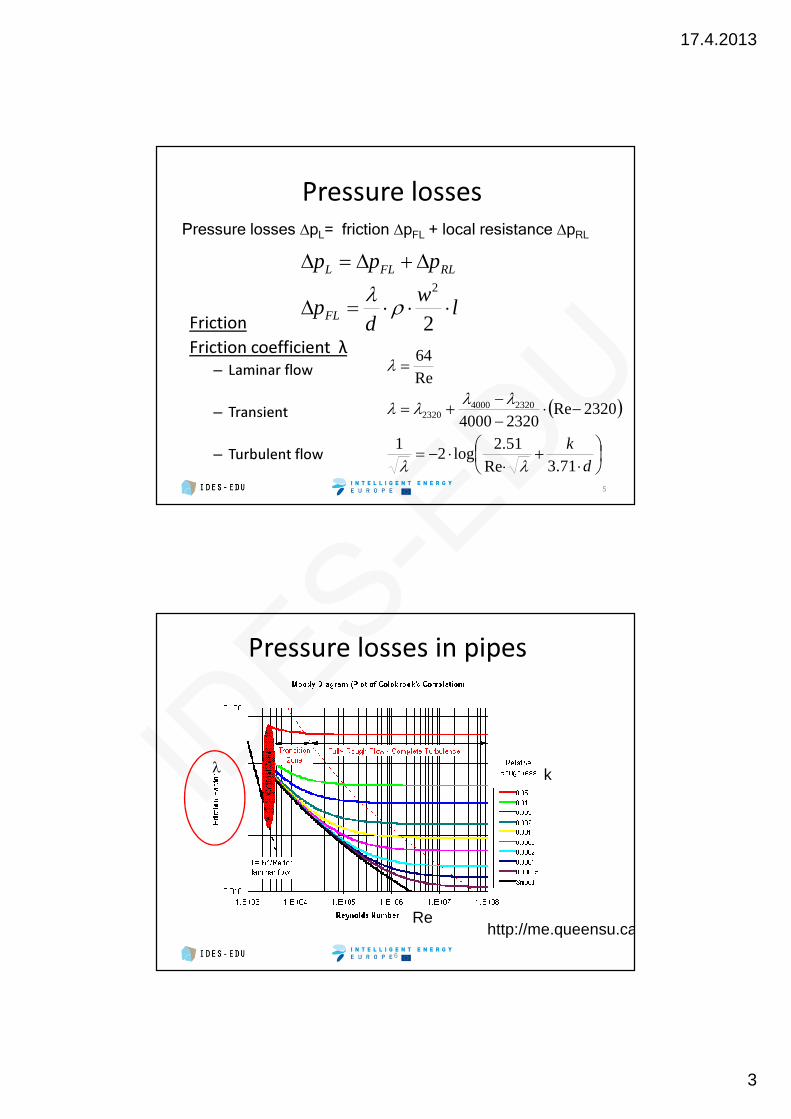
Pressure losses

FrictionFriction coefficient λ

– Laminar flow

– Transient

– Turbulent flow5

Pressure losses ∆pL= friction ∆pFL + local resistance ∆pRL

RLFLL ppp ∆+∆=∆

lw

dpFL ⋅⋅⋅=∆

2

2

ρλ

( )

⋅+⋅⋅−=

−⋅−−+=

=

d

k

71.3Re

51.2log2

1

2320Re23204000

Re64

232040002320

λλ

λλλλ

λ

Pressure losses in pipes

6

http://me.queensu.ca

k

Re

λIDES-E

DU

17.4.2013

4

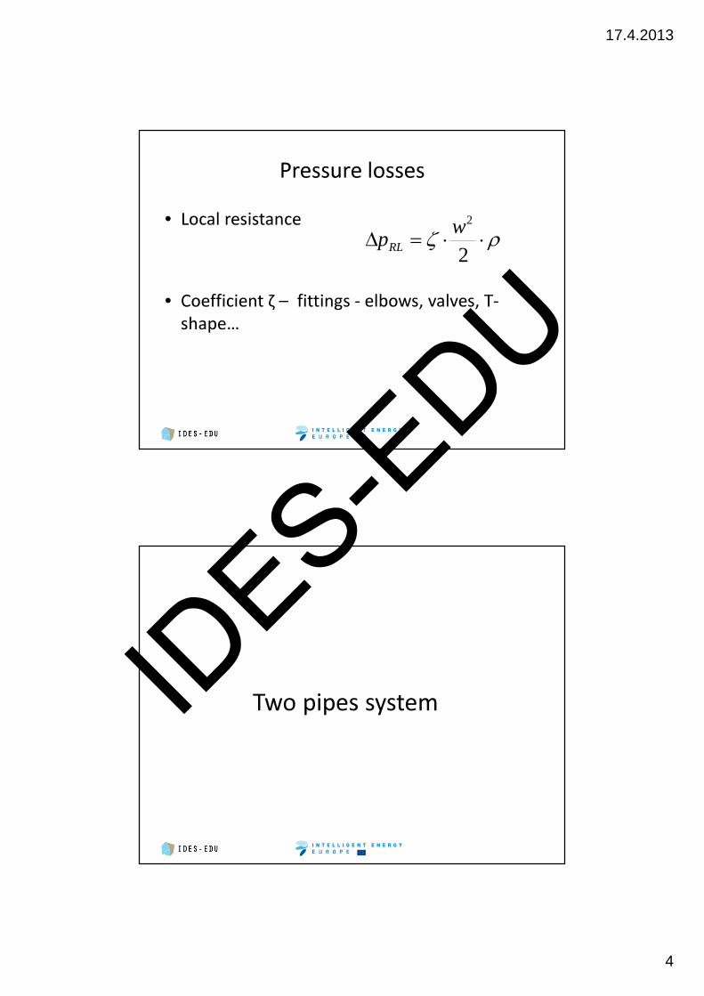
Pressure losses• Local resistance

• Coefficient ζ – fittings - elbows, valves, T-shape…

7

ρζ ⋅⋅=∆2

2wpRL

Two pipes systemIDES-E

DU

17.4.2013

5

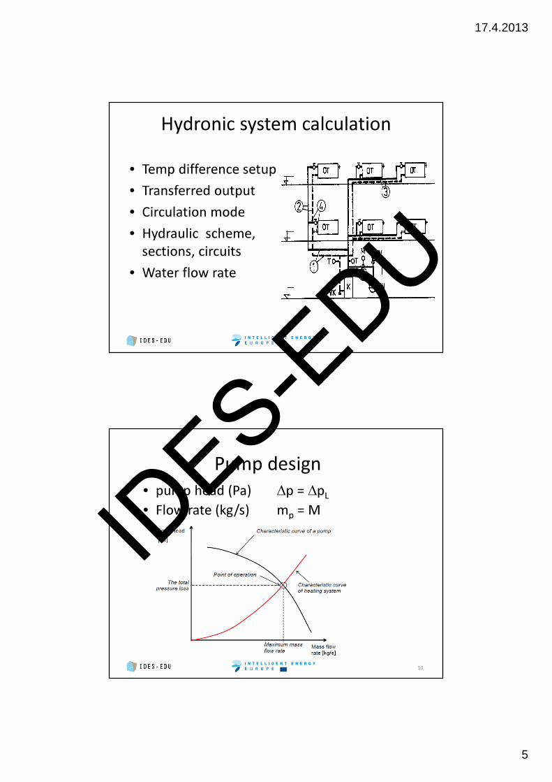
Hydronic system calculation• Temp difference setup• Transferred output• Circulation mode• Hydraulic scheme,

sections, circuits• Water flow rate

Pump design• pump head (Pa) ∆p = ∆pL• Flow rate (kg/s) mp = M

10

IDES-E

DU

17.4.2013

6

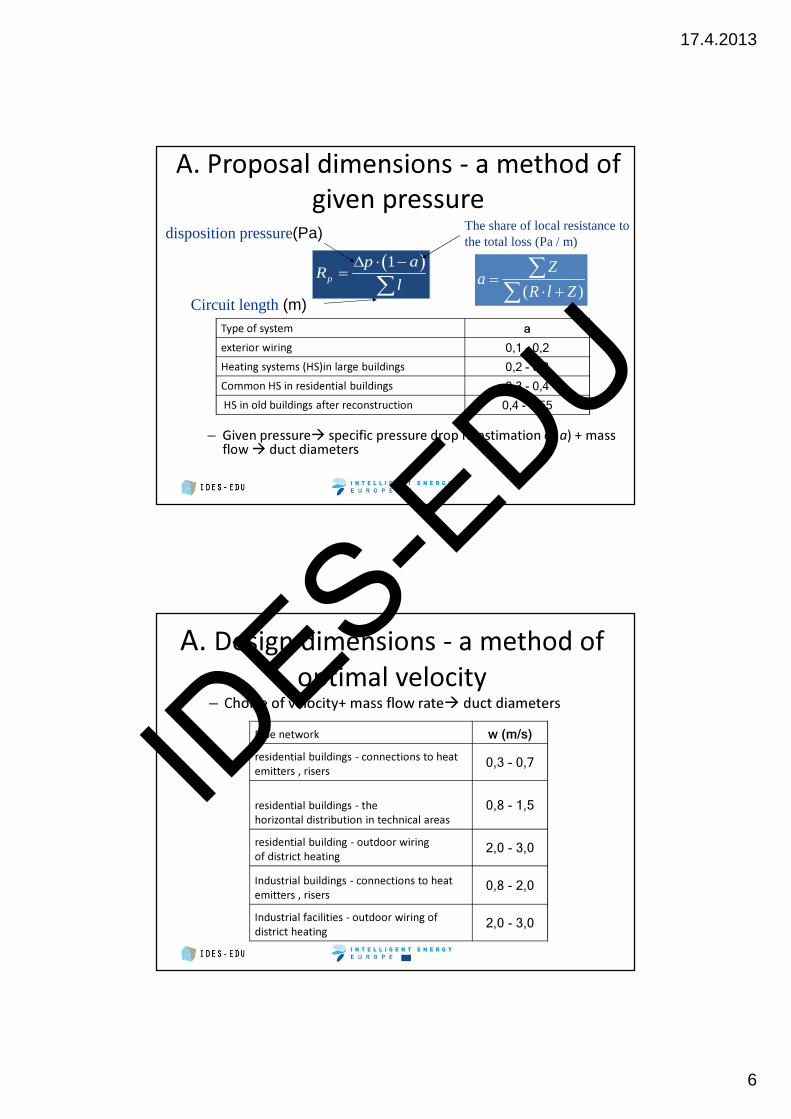
A. Proposal dimensions - a method ofgiven pressure

( )1p

p aR

l

∆ ⋅ −= ∑

disposition pressure(Pa)

Circuit length (m)

The share of local resistance to the total loss (Pa / m)

( )

Za

R l Z=

⋅ +∑∑

Type of system a

exterior wiring 0,1 - 0,2Heating systems (HS)in large buildings 0,2 - 0,3Common HS in residential buildings 0,3 - 0,4HS in old buildings after reconstruction 0,4 - 0,55

– Given pressure� specific pressure drop R (estimation of a) + massflow� duct diameters

A. Design dimensions - a method of optimal velocity

– Choice of velocity+ mass flow rate� duct diametersPipe network w (m/s)residential buildings - connections to heatemitters , risers 0,3 - 0,7

residential buildings - the horizontal distribution in technical areas

0,8 - 1,5

residential building - outdoor wiringof district heating 2,0 - 3,0

Industrial buildings - connections to heatemitters , risers 0,8 - 2,0

Industrial facilities - outdoor wiring ofdistrict heating 2,0 - 3,0

IDES-E

DU

17.4.2013

7

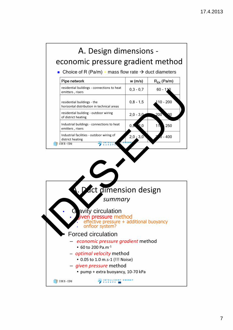
A. Design dimensions -economic pressure gradient method� Choice of R (Pa/m) + mass flow rate� duct diameters

Pipe network w (m/s) REK (Pa/m)residential buildings - connections to heatemitters , risers 0,3 - 0,7 60 - 110

residential buildings - the horizontal distribution in technical areas

0,8 - 1,5 110 - 200

residential building - outdoor wiringof district heating 2,0 - 3,0 200 - 400

Industrial buildings - connections to heatemitters , risers 0,8 - 2,0 110 - 250

Industrial facilities - outdoor wiring ofdistrict heating 2,0 - 3,0 200 - 400

A. Duct dimension designsummary

• Forced circulation– economic pressure gradient method

• 60 to 200 Pa.m-1

– optimal velocity method• 0.05 to 1.0 m.s-1 (!!! Noise)

– given pressure method• pump + extra buoyancy, 10-70 kPa

• Gravity circulation• given pressure method

• effective pressure + additional buoyancy• onfloor system?IDES-E

DU

17.4.2013

8

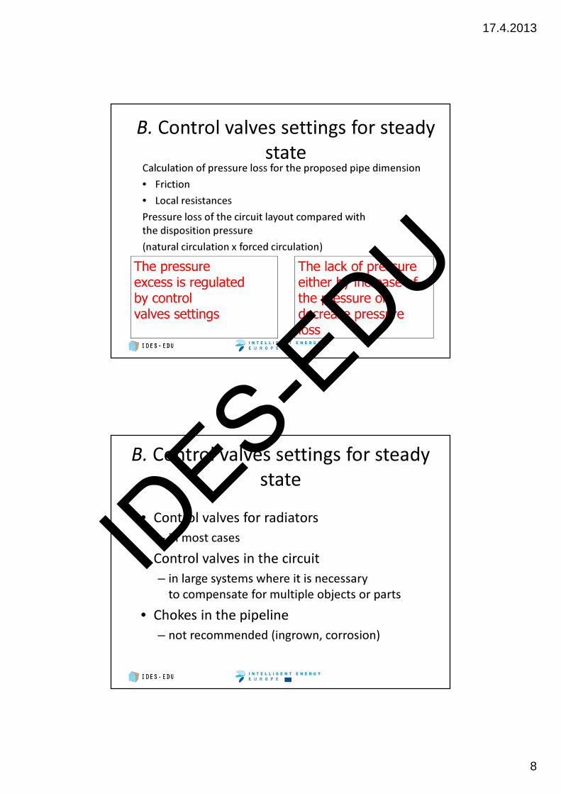
B. Control valves settings for steady state

Calculation of pressure loss for the proposed pipe dimension• Friction• Local resistancesPressure loss of the circuit layout compared with the disposition pressure(natural circulation x forced circulation)

The pressureexcess is regulated by control valves settings

The lack of pressureeither by increase ofthe pressure ordecrease pressureloss

B. Control valves settings for steady state

• Control valves for radiators– in most cases

• Control valves in the circuit– in large systems where it is necessary

to compensate for multiple objects or parts• Chokes in the pipeline

– not recommended (ingrown, corrosion)

IDES-E

DU

17.4.2013

9

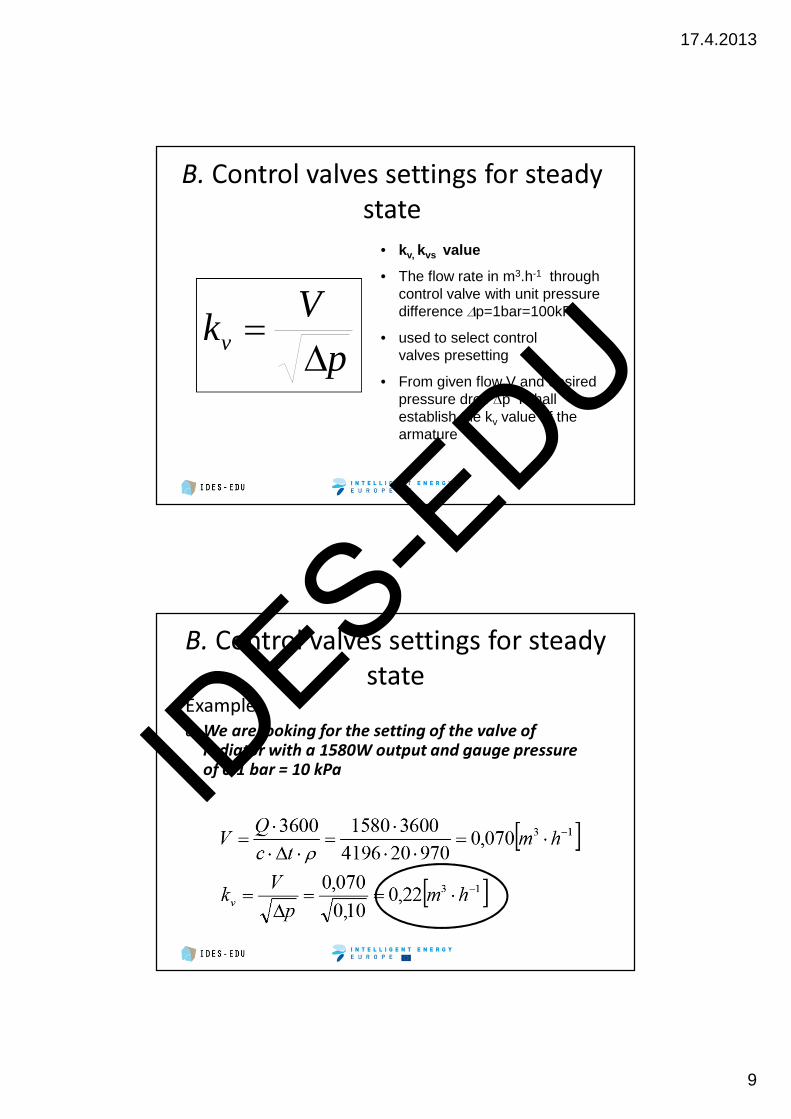
B. Control valves settings for steady state

• kv, kvs value

• The flow rate in m3.h-1 throughcontrol valve with unit pressure difference ∆p=1bar=100kPa

• used to select control valves presetting

• From given flow V and desiredpressure drop ∆p I shall establish the kv value of thearmature

p

Vkv ∆

=

B. Control valves settings for steady state

Example: â We are looking for the setting of the valve of

radiator with a 1580W output and gauge pressureof 0.1 bar = 10 kPaID

ES-EDU

17.4.2013

10

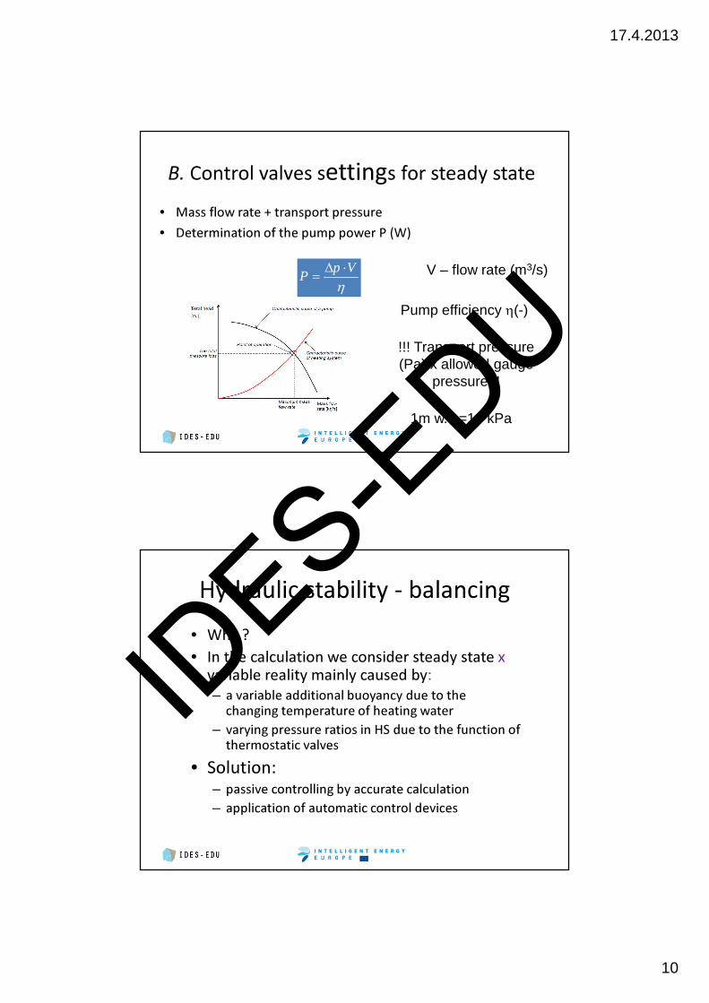
B. Control valves settings for steady state• Mass flow rate + transport pressure• Determination of the pump power P (W)

p VP

η∆ ⋅= V – flow rate (m3/s)

!!! Transport pressure(Pa) x allowed gauge

pressure!!!

1m w.c.=10 kPa

Pump efficiency η(-)

Hydraulic stability - balancing• Why ?• In the calculation we consider steady state x

variable reality mainly caused by: – a variable additional buoyancy due to the

changing temperature of heating water– varying pressure ratios in HS due to the function of

thermostatic valves• Solution:

– passive controlling by accurate calculation– application of automatic control devices

IDES-E

DU

17.4.2013

11

Hydraulic stability - balancing • Passive – by the calculation

– rules for the design of individual parts of HS– E.g. for systems with gravity circulation::

• consume the most pressure on heat emitters• pressure drop in the riser = effective

pressure merged in the riser• pressure loss in horizontal distribution

systems = effective pressuremerged in horizontal distribution systems

– numerically difficult, the problem of realization

Hydraulic stability - balancing• Applications of automatic control devices

– bypass valves• opens with variations according to the

differential pressure, placed to bypass of the pump or between the supply and return piping of HS

• differential pressure regulators• strangling (!) valve in the pipe controlled by

differential pressure• pump with controlled speed• Constant pump pressure within variable flow

IDES-E

DU

17.4.2013

12

One pipe heating systems

One pipe heating systems• Calculation

– Temperature - Determinestemperatures in individual heat emitters undercomputational conditions

– Hydraulic - defines the set of valves, pipe dimensions and parameters of the pump

IDES-E

DU

17.4.2013

13

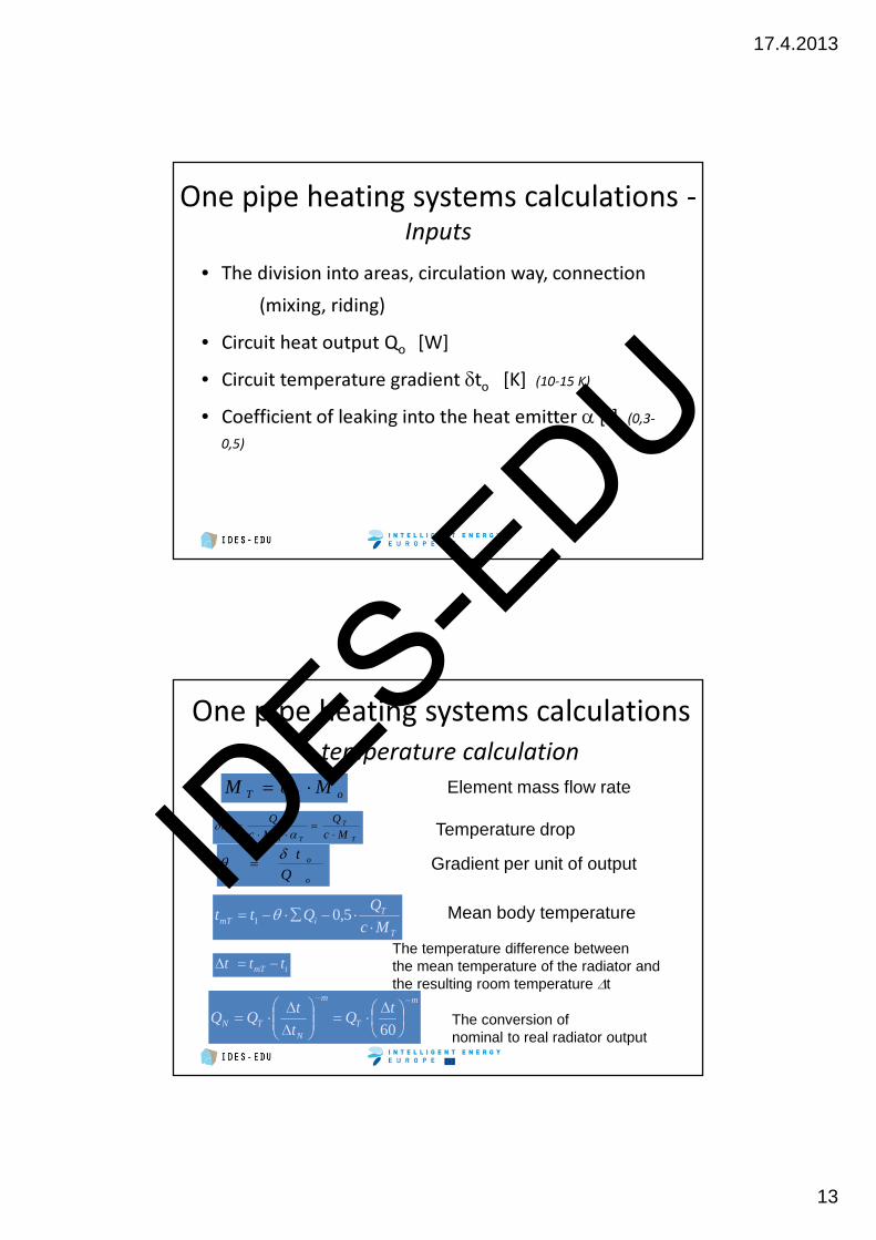
One pipe heating systems calculations -Inputs

• The division into areas, circulation way, connection(mixing, riding)

• Circuit heat output Qo [W] • Circuit temperature gradient δto [K] (10-15 K)

• Coefficient of leaking into the heat emitter α [-] (0,3-0,5)

One pipe heating systems calculations- temperature calculation

oTT MαM ⋅= Element mass flow rate

T

T

To

TT Mc

QMc

Qt

⋅=

⋅⋅=

αδ Temperature drop

T

TimT Mc

QQtt ⋅⋅−∑⋅−= 5,01 θ

m

T

m

NTN

tQ

t

tQQ

−−

∆⋅=

∆∆⋅=

60

imT ttt −=∆

o

o

Q

tδθ = Gradient per unit of output

Mean body temperature

The temperature difference between the mean temperature of the radiator and the resulting room temperature ∆t

The conversion of nominal to real radiator output

IDES-E

DU

17.4.2013

14

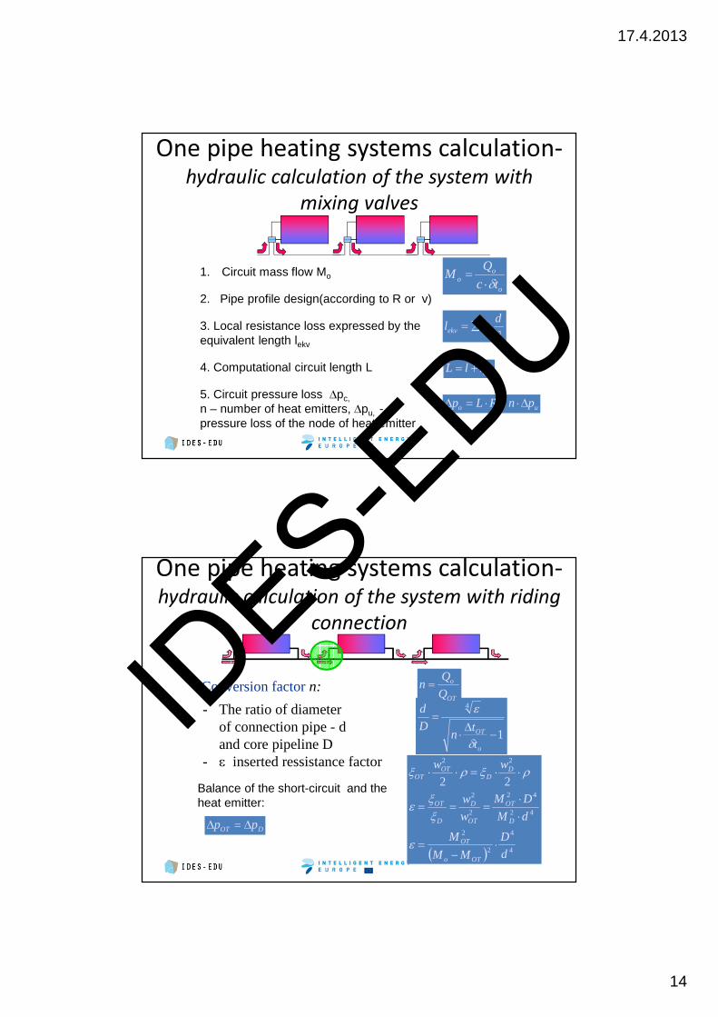
One pipe heating systems calculation-hydraulic calculation of the system with

mixing valves

o

oo tc

QM

δ⋅=1. Circuit mass flow Mo

uo pnRLp ∆⋅+⋅=∆5. Circuit pressure loss ∆pc, n – number of heat emitters, ∆pu, -pressure loss of the node of heat emitter

λξ dlekv ⋅∑=3. Local resistance loss expressed by the

equivalent length lekv

2. Pipe profile design(according to R or v)

ekvllL +=4. Computational circuit length L

One pipe heating systems calculation-hydraulic calculation of the system with riding

connection

DOT pp ∆=∆

( ) 4

4

2

2

42

42

2

2

22

22

d

D

MM

M

dM

DM

w

w

ww

OTo

OT

D

OT

OT

D

D

OT

DD

OTOT

⋅−

=

⋅

⋅===

⋅⋅=⋅⋅

εξξε

ρξρξ

1

4

−∆⋅=

o

OT

t

tn

D

d

δ

ε- The ratio of diameter of connection pipe - d and core pipeline D

- ε inserted ressistance factor

OT

o

Q

Qn =Conversion factor n:

Balance of the short-circuit and theheat emitter:

IDES-E

DU

17.4.2013

15

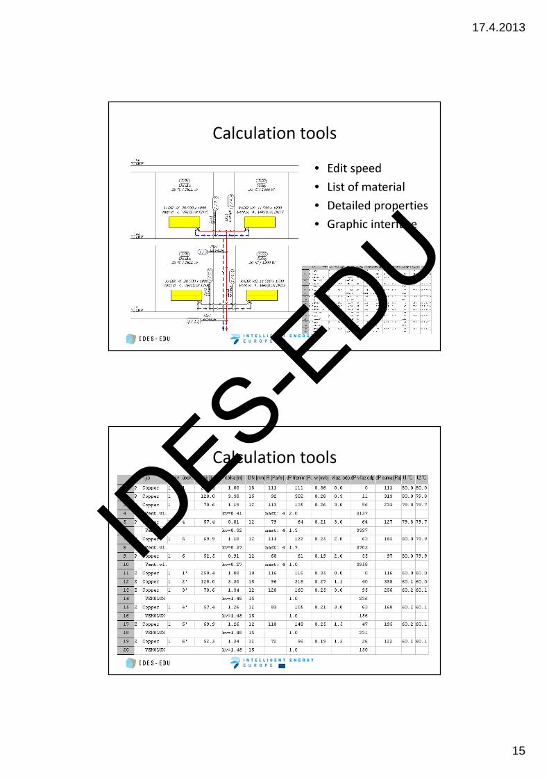
Calculation tools• Edit speed• List of material• Detailed properties• Graphic interface

Calculation tools

IDES-E

DU

17.4.2013

16

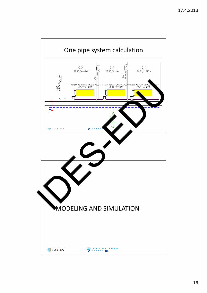
One pipe system calculation

MODELING AND SIMULATIONIDES-E

DU

17.4.2013

17

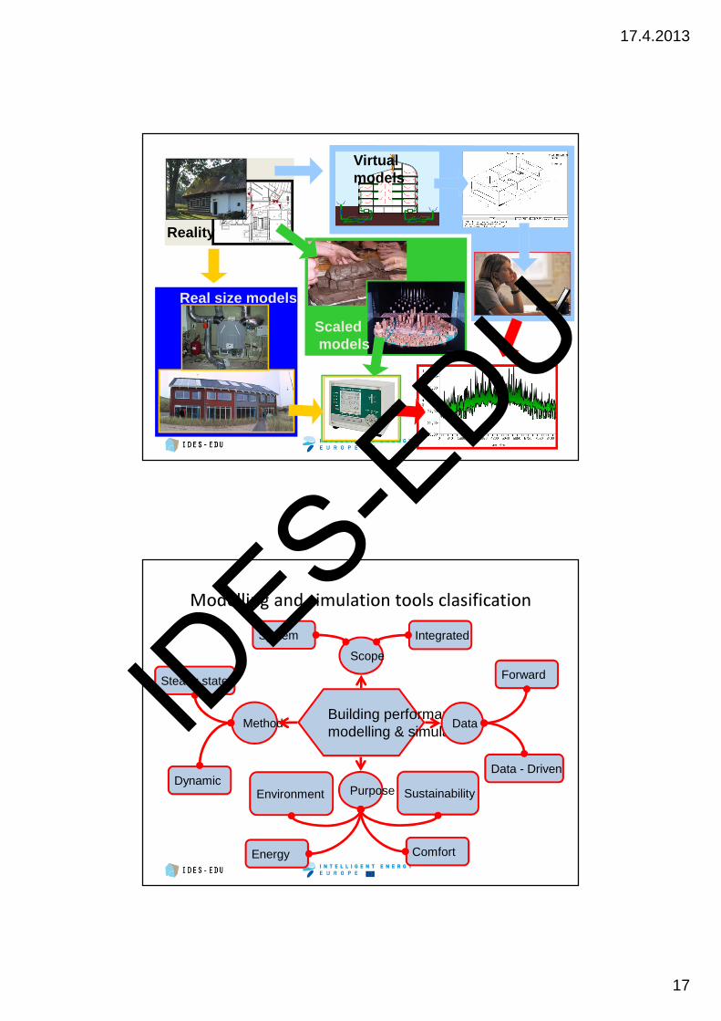
Reality

Real size models

Scaledmodels

Fig. 3. ESP-r model of the building

Fig. 3. ESP-r model of the building

Virtual models

Modelling and simulation tools clasification

Building performance modelling & simulation

Method

Steady state

Dynamic

Scope

System Integrated

Data

Forward

Data - Driven

Purpose

Energy Comfort

Environment Sustainability

IDES-E

DU

17.4.2013

18

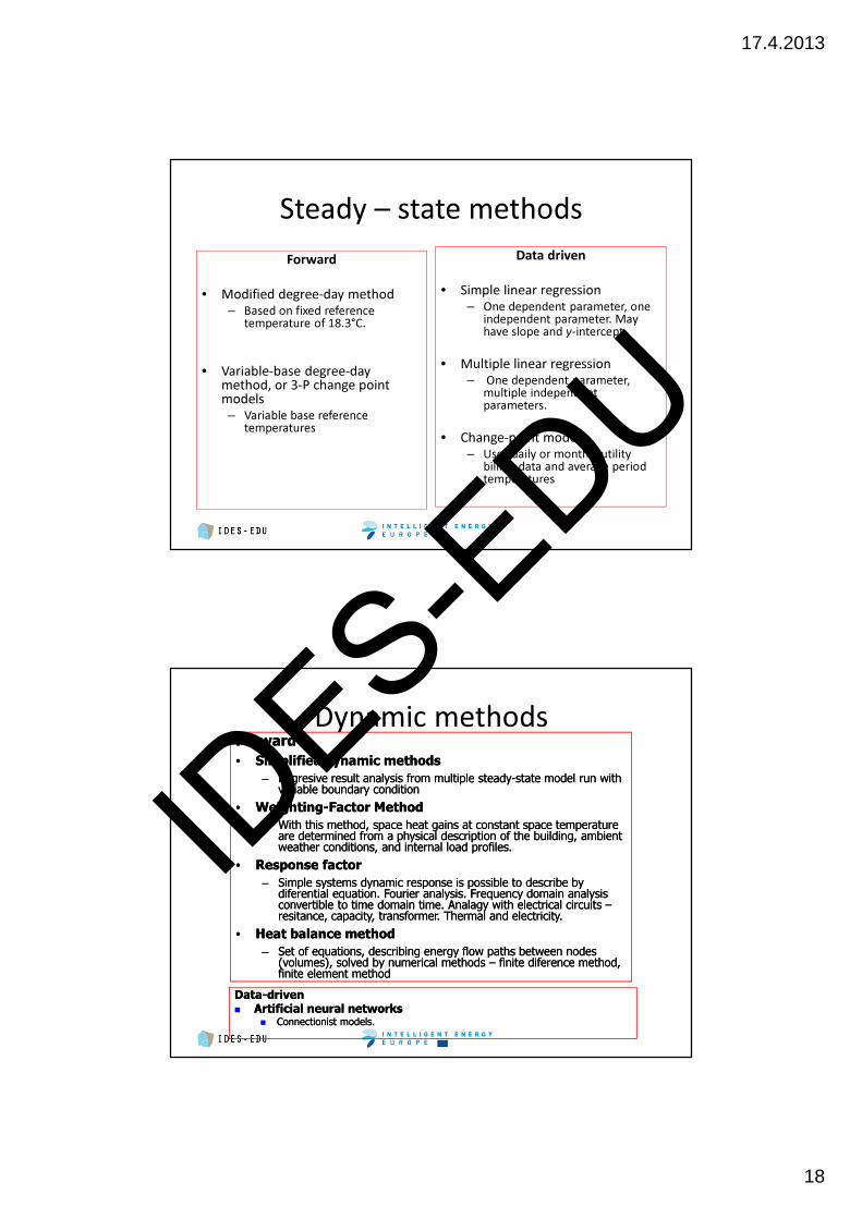
Steady – state methodsForward

• Modified degree-day method– Based on fixed reference

temperature of 18.3°C.

• Variable-base degree-daymethod, or 3-P change point models– Variable base reference

temperatures

Data driven

• Simple linear regression– One dependent parameter, one

independent parameter. May have slope and y-intercept

• Multiple linear regression– One dependent parameter,

multiple independentparameters.

• Change-point models– Uses daily or monthly utility

billing data and average period temperatures

Dynamic methodsForward• Simplified dynamic methods

– Regresive result analysis from multiple steady-state model run with variable boundary condition• Weighting-Factor Method

– With this method, space heat gains at constant space temperature are determined from a physical description of the building, ambient weather conditions, and internal load profiles.• Response factor

– Simple systems dynamic response is possible to describe by diferential equation. Fourier analysis. Frequency domain analysis convertible to time domain time. Analagy with electrical circuits –resitance, capacity, transformer. Thermal and electricity.• Heat balance method

– Set of equations, describing energy flow paths between nodes (volumes), solved by numerical methods – finite diference method, finite element method

Forward• Simplified dynamic methods

– Regresive result analysis from multiple steady-state model run with variable boundary condition• Weighting-Factor Method

– With this method, space heat gains at constant space temperature are determined from a physical description of the building, ambient weather conditions, and internal load profiles.• Response factor

– Simple systems dynamic response is possible to describe by diferential equation. Fourier analysis. Frequency domain analysis convertible to time domain time. Analagy with electrical circuits –resitance, capacity, transformer. Thermal and electricity.• Heat balance method

– Set of equations, describing energy flow paths between nodes (volumes), solved by numerical methods – finite diference method, finite element methodData-driven� Artificial neural networks

� Connectionist models.

Data-driven� Artificial neural networks

� Connectionist models.

IDES-E

DU

17.4.2013

19

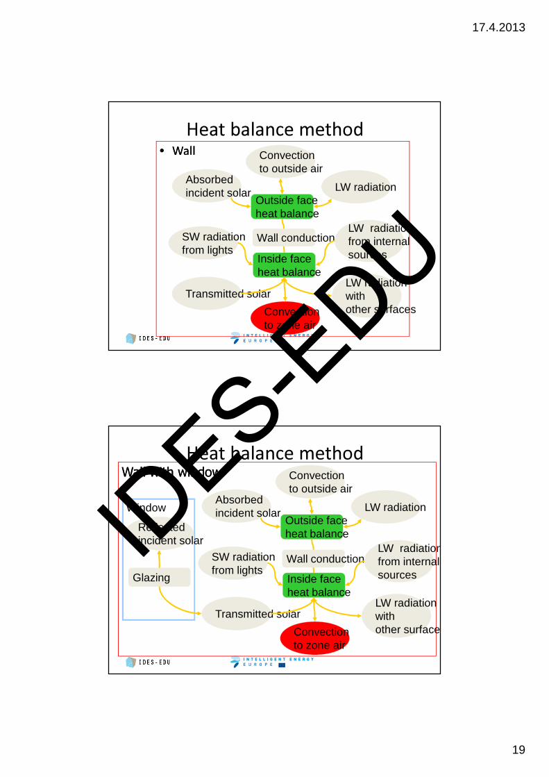
Heat balance method• Wall• Wall

Outside face heat balance

Absorbed incident solar

Convection to outside air

LW radiation

Wall conduction

Inside face heat balance

SW radiation from lights

Transmitted solarLW radiation with other surfaces

LW radiation from internal sources

Convection to zone air

Heat balance methodWall with windowWall with window

Outside face heat balance

Absorbed incident solar

Convection to outside air

LW radiation

Wall conduction

Inside face heat balance

SW radiation from lights

Transmitted solarLW radiation with other surfaces

LW radiation from internal sources

Convection to zone air

Window

Reflectedincident solar

Glazing

IDES-E

DU

17.4.2013

20

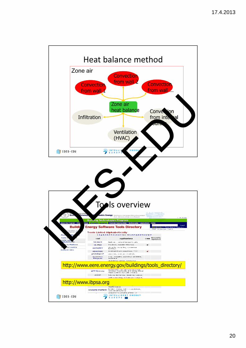
Heat balance methodZone air

Zone air heat balanceZone air heat balance

Infiltration

Ventilation (HVAC)Ventilation (HVAC)

Convection from internal sourcesConvection from internal sources

Convection from wall 2Convection from wall 2Convection

from wall 1Convection from wall 1

Convection from wall …Convection from wall …

Tools overview

http://www.eere.energy.gov/buildings/tools_directory/

http://www.ibpsa.org

IDES-E

DU

17.4.2013

21

ESP-RBuilding Energy Performance Simulation

ESP-r background• ESP-r (Environmental Systems Performance;

r for "research„)• Dynamic, whole building simulation finite volume,

finite difference sw based on heat balance method.• Academic, research / non commercial• Developed at ESRU, Dept.of Mech. Eng. University of

Strathclyde, Glasgow, UK by prof. Joseph Clarke and his team since 1974

• ESP-r is released under the terms of the GNU General Public License. It can be used for commercial or non-commercial work subject to the terms of this open source licence agreement.

• UNIX, Cygwin, Windows

http://www.esru.strath.ac.uk/

IDES-E

DU

17.4.2013

22

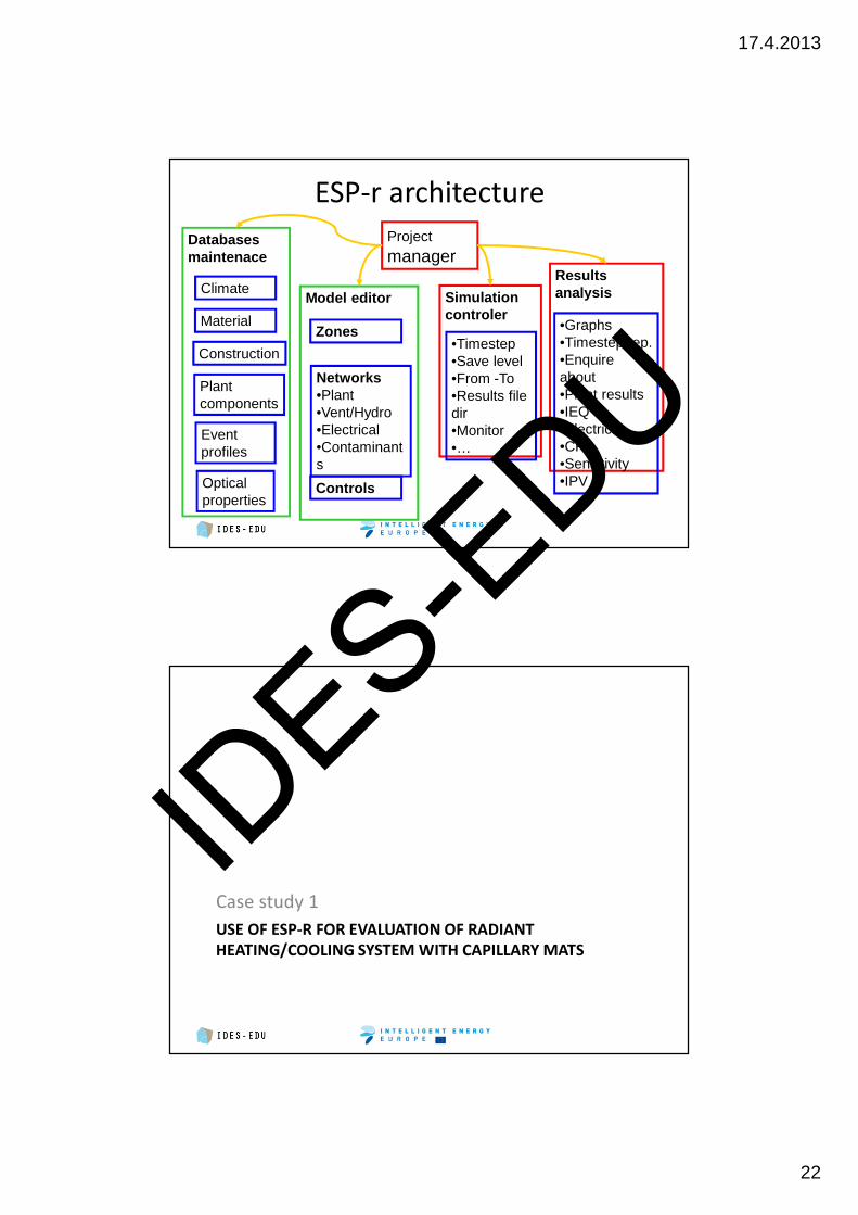
ESP-r architectureProject

manager

Climate

Material

Construction

Plant components

Event profiles

Optical properties

Databases maintenace

Model editor

Zones

Networks•Plant•Vent/Hydro•Electrical•Contaminants

Controls

Simulation controler

Resultsanalysis

•Timestep•Save level•From -To•Results file dir•Monitor•…

•Graphs•Timestep rep.•Enquire about•Plant results•IEQ•Electrical•CFD•Sensitivity•IPV

USE OF ESP-R FOR EVALUATION OF RADIANT HEATING/COOLING SYSTEM WITH CAPILLARY MATS

Case study 1ID

ES-EDU

17.4.2013

23

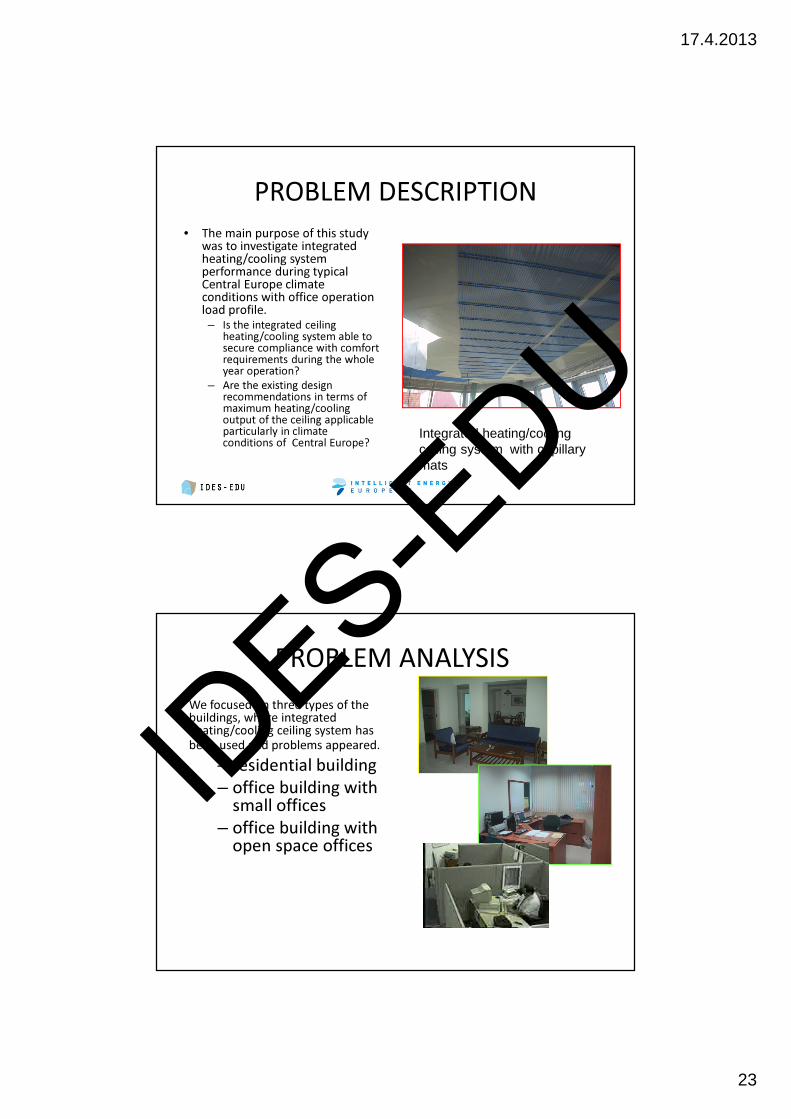
PROBLEM DESCRIPTION• The main purpose of this study

was to investigate integrated heating/cooling system performance during typical Central Europe climate conditions with office operation load profile. – Is the integrated ceiling

heating/cooling system able to secure compliance with comfort requirements during the whole year operation?

– Are the existing design recommendations in terms of maximum heating/cooling output of the ceiling applicable particularly in climate conditions of Central Europe? Integrated heating/cooling

ceiling system with capillarymats

PROBLEM ANALYSISWe focused on three types of the buildings, where integrated heating/cooling ceiling system has been used and problems appeared.

– residential building– office building with

small offices – office building with

open space officesID

ES-EDU

17.4.2013

24

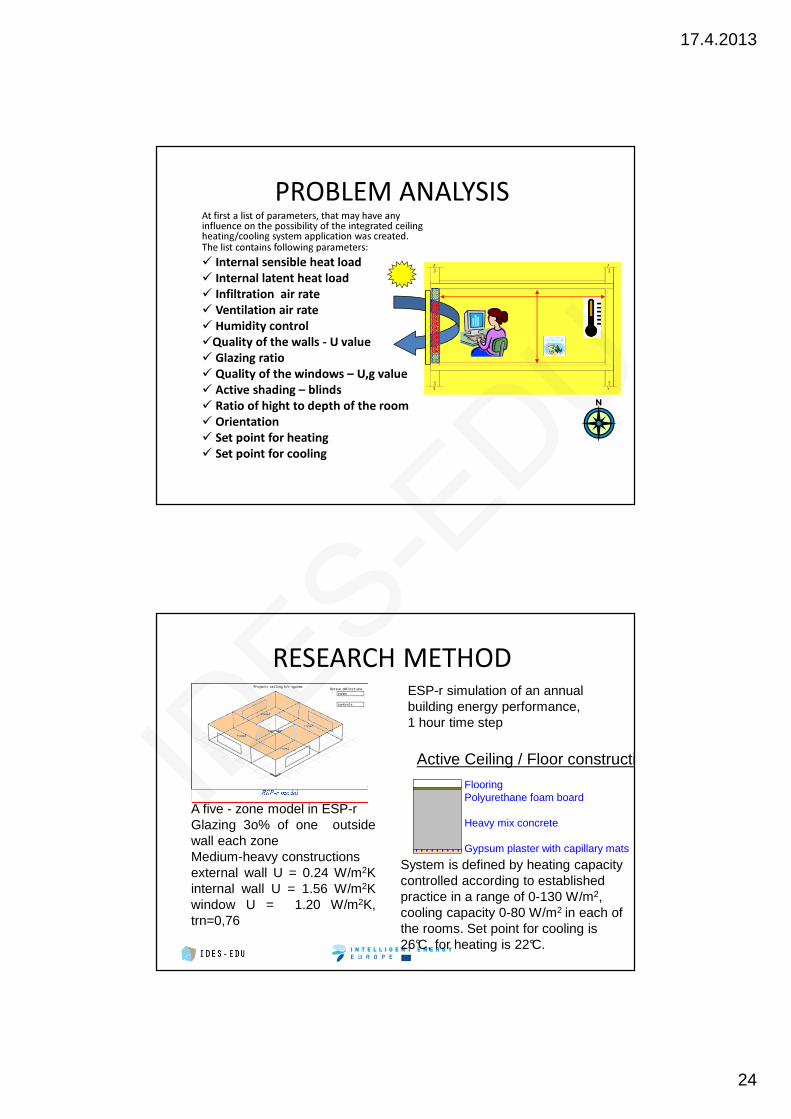
PROBLEM ANALYSISAt first a list of parameters, that may have any influence on the possibility of the integrated ceiling heating/cooling system application was created. The list contains following parameters:� Internal sensible heat load� Internal latent heat load � Infiltration air rate� Ventilation air rate� Humidity control�Quality of the walls - U value� Glazing ratio� Quality of the windows – U,g value� Active shading – blinds� Ratio of hight to depth of the room� Orientation� Set point for heating� Set point for cooling

RESEARCH METHOD

A five - zone model in ESP-rGlazing 3o% of one outsidewall each zoneMedium-heavy constructionsexternal wall U = 0.24 W/m2Kinternal wall U = 1.56 W/m2Kwindow U = 1.20 W/m2K,trn=0,76

ESP-r simulation of an annual building energy performance, 1 hour time step

FlooringPolyurethane foam board

Heavy mix concrete

Gypsum plaster with capillary mats

Active Ceiling / Floor construction

System is defined by heating capacity controlled according to established practice in a range of 0-130 W/m2, cooling capacity 0-80 W/m2 in each of the rooms. Set point for cooling is 26°C, for heating is 22°C.

IDES-E

DU

17.4.2013

25

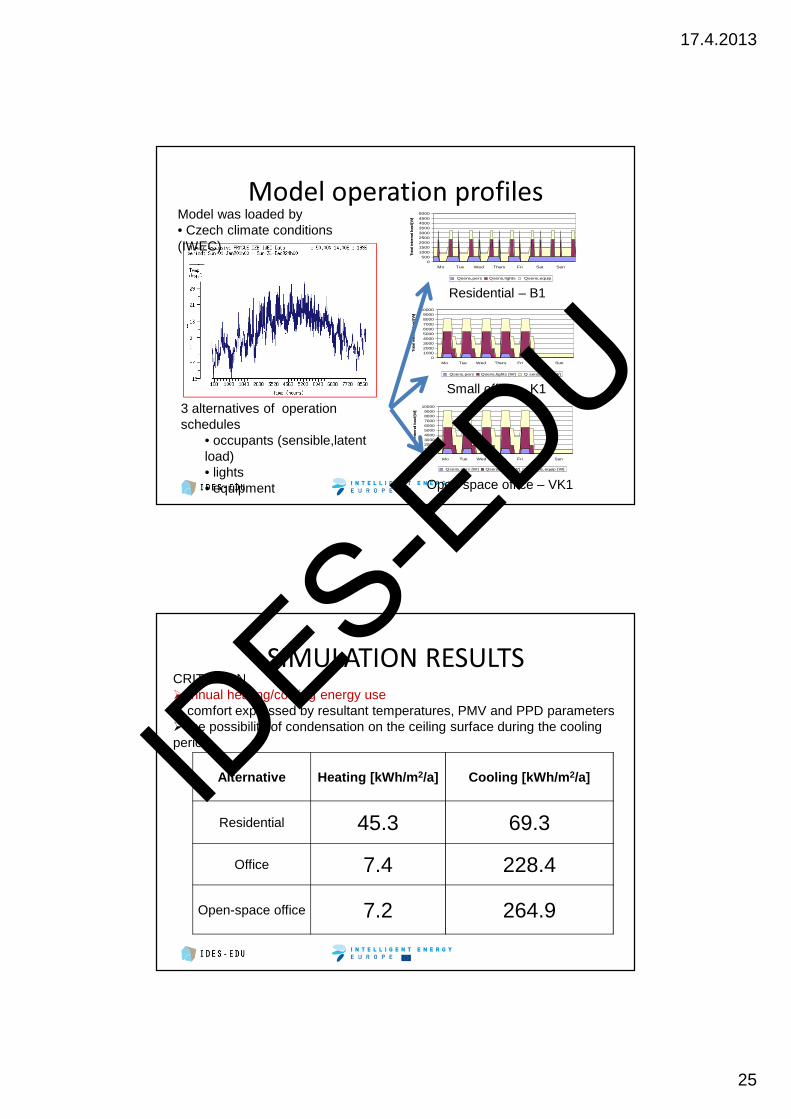
Model operation profilesModel was loaded by • Czech climate conditions(IWEC)

0500

100015002000250030003500400045005000

Mo Tue Wed Thurs Fri Sat Sun

Tot

al int

ernal

load

[W

]

Qsens,pers Qsens,lights Qsens,equip

0100020003000400050006000700080009000

10000

Mo Tue Wed Thurs Fri Sat Sun

Tot

al in

tern

al lo

ad [W

]

Qsens,pers Qsens,lights [W] Q sens,equip [W]

0100020003000400050006000700080009000

10000

Mo Tue Wed Thurs Fri Sat Sun

Tot

al in

tern

al lo

ad [W

]

Qsens,pers [W] Qsens,lights [W] Q sens,equip [W]

Residential – B1

Small office – K1

Open space office – VK1

3 alternatives of operationschedules

• occupants (sensible,latentload)• lights• equipment

SIMULATION RESULTS

Alternative Heating [kWh/m2/a] Cooling [kWh/m2/a]

Residential 45.3 69.3

Office 7.4 228.4

Open-space office 7.2 264.9

CRITERION �annual heating/cooling energy use� comfort expressed by resultant temperatures, PMV and PPD parameters� the possibility of condensation on the ceiling surface during the cooling periodID

ES-EDU

17.4.2013

26

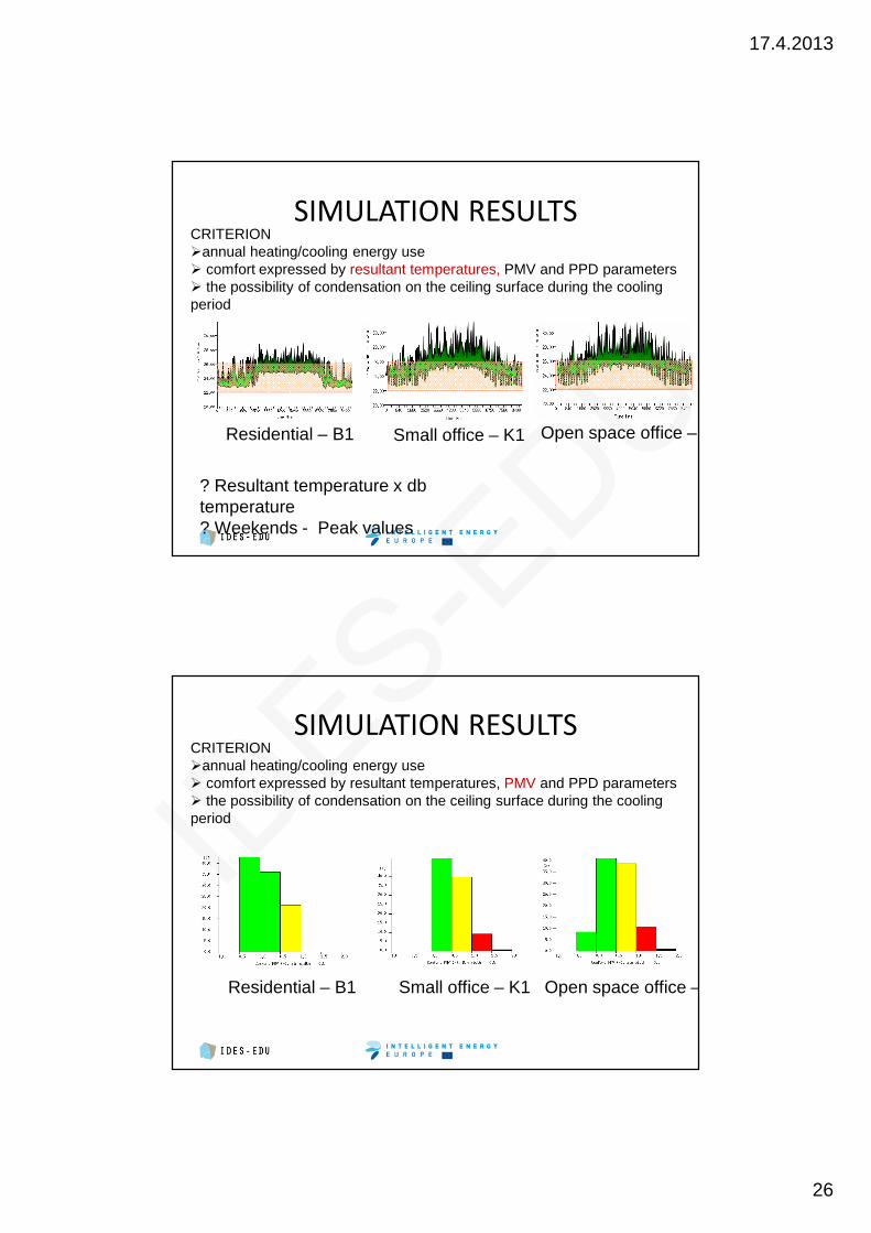
SIMULATION RESULTS

Residential – B1 Small office – K1 Open space office –

? Resultant temperature x db temperature? Weekends - Peak values

CRITERION �annual heating/cooling energy use� comfort expressed by resultant temperatures, PMV and PPD parameters� the possibility of condensation on the ceiling surface during the cooling period

SIMULATION RESULTS

Residential – B1 Small office – K1 Open space office –

CRITERION �annual heating/cooling energy use� comfort expressed by resultant temperatures, PMV and PPD parameters� the possibility of condensation on the ceiling surface during the cooling periodID

ES-EDU

17.4.2013

27

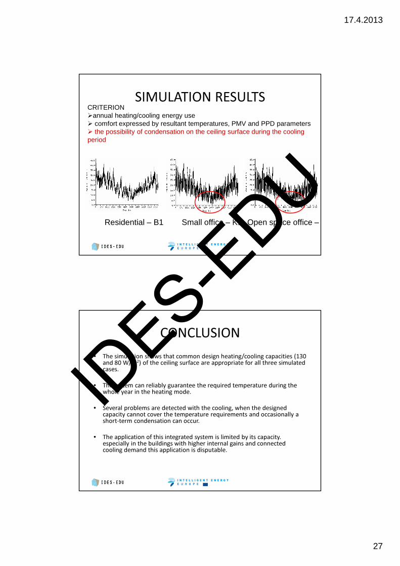
SIMULATION RESULTS

Residential – B1 Small office – K1 Open space office – VK1

CRITERION �annual heating/cooling energy use� comfort expressed by resultant temperatures, PMV and PPD parameters� the possibility of condensation on the ceiling surface during the cooling period

CONCLUSION• The simulation shows that common design heating/cooling capacities (130

and 80 W/m2) of the ceiling surface are appropriate for all three simulated cases.

• The system can reliably guarantee the required temperature during the whole year in the heating mode.

• Several problems are detected with the cooling, when the designed capacity cannot cover the temperature requirements and occasionally a short-term condensation can occur.

• The application of this integrated system is limited by its capacity. especially in the buildings with higher internal gains and connected cooling demand this application is disputable.

IDES-E

DU

17.4.2013

28

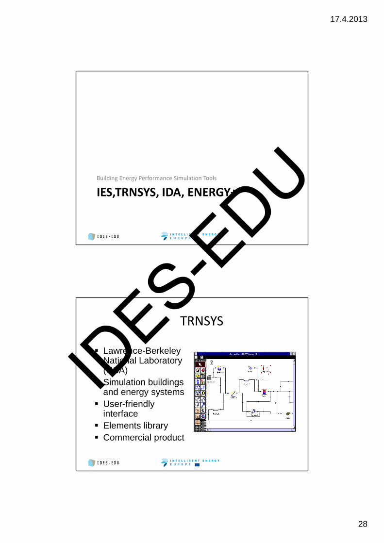
IES,TRNSYS, IDA, ENERGY+Building Energy Performance Simulation Tools

TRNSYS� Lawrence-Berkeley

National Laboratory (USA)

� Simulation buildings and energy systems

� User-friendly interface

� Elements library� Commercial product

IDES-E

DU

17.4.2013

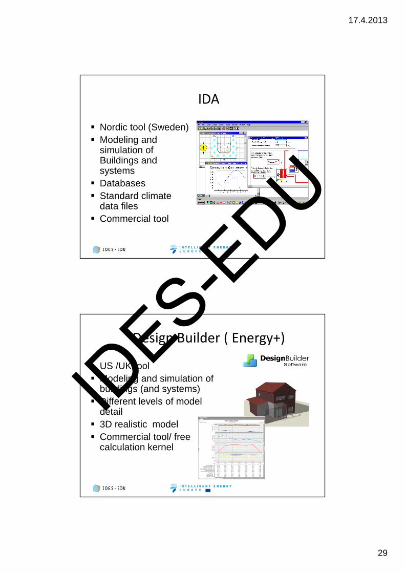
29

IDA � Nordic tool (Sweden)� Modeling and

simulation of Buildings and systems

� Databases� Standard climate

data files� Commercial tool

Design Builder ( Energy+) � US /UK tool� Modeling and simulation of

buildings (and systems)� Different levels of model

detail� 3D realistic model� Commercial tool/ free

calculation kernel

IDES-E

DU

17.4.2013

30

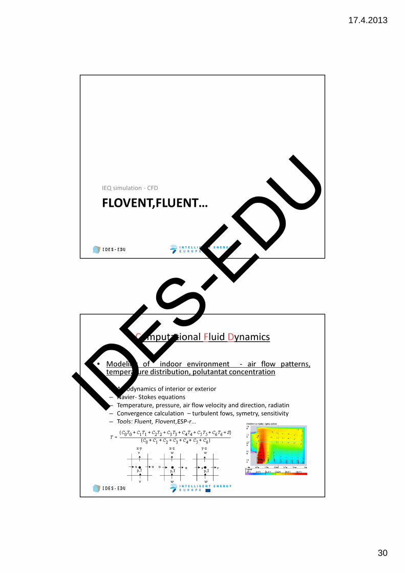
FLOVENT,FLUENT…IEQ simulation - CFD

Computational Fluid Dynamics

• Modeling of indoor environment - air flow patterns,temperature distribution, polutantat concentration– Aerodynamics of interior or exterior– Navier- Stokes equations– Temperature, pressure, air flow velocity and direction, radiatin– Convergence calculation – turbulent fows, symetry, sensitivity– Tools: Fluent, Flovent,ESP-r…ID

ES-EDU

17.4.2013

31

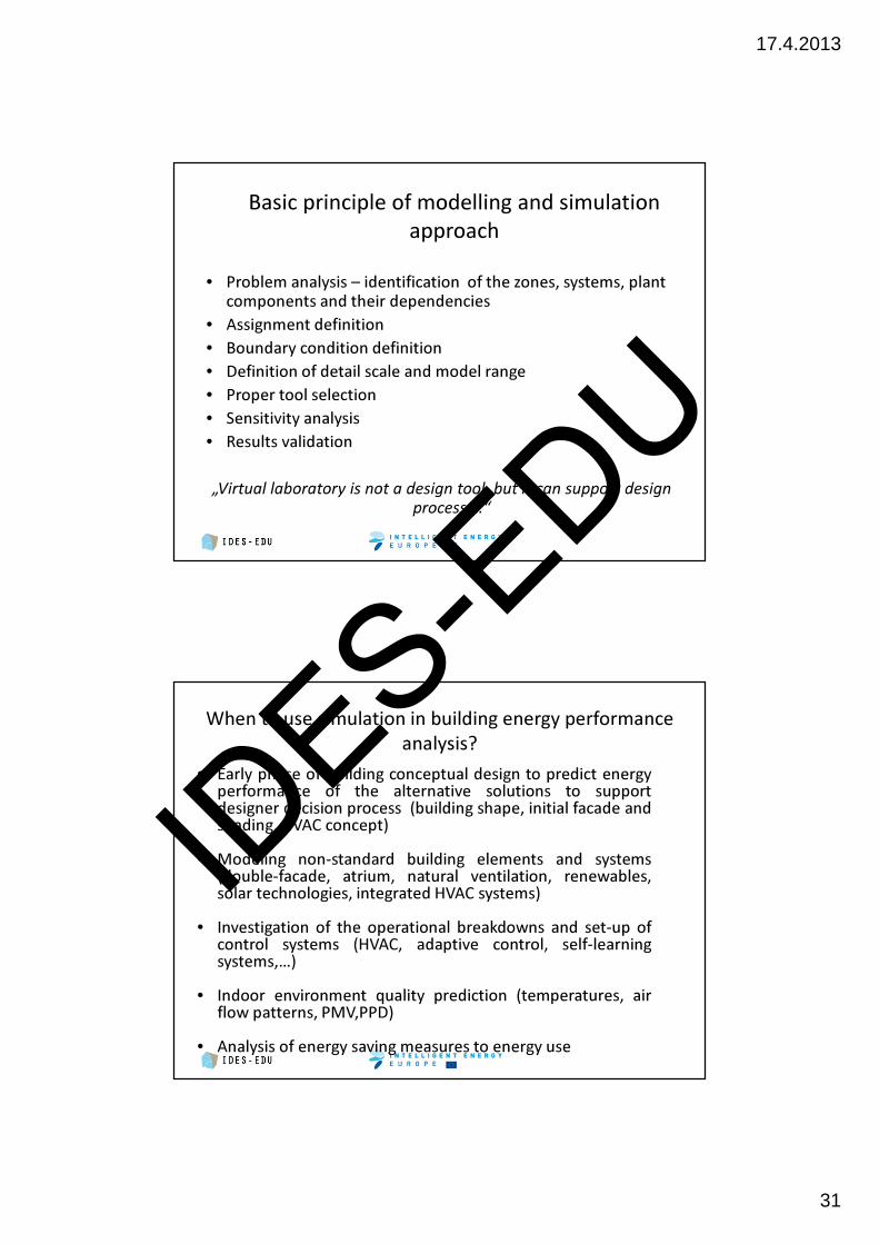
Basic principle of modelling and simulationapproach

• Problem analysis – identification of the zones, systems, plant components and their dependencies

• Assignment definition• Boundary condition definition• Definition of detail scale and model range • Proper tool selection• Sensitivity analysis• Results validation

„Virtual laboratory is not a design tool, but it can support design process …“

When to use simulation in building energy performance analysis?

• Early phase of building conceptual design to predict energyperformance of the alternative solutions to supportdesigner decision process (building shape, initial facade andshading, HVAC concept)

• Modeling non-standard building elements and systems(double-facade, atrium, natural ventilation, renewables,solar technologies, integrated HVAC systems)

• Investigation of the operational breakdowns and set-up ofcontrol systems (HVAC, adaptive control, self-learningsystems,…)

• Indoor environment quality prediction (temperatures, airflow patterns, PMV,PPD)

• Analysis of energy saving measures to energy use

IDES-E

DU

17.4.2013

32

References and relevant bibliography

• Kabele, K. - Dvořáková, P. Multicriterion evaluation of anintegrated sustainable heating/cooling system in climateconditions of Central Europe In: BS 2007 [CD-ROM]. Beijing:

Tsinghua University, 2007, vol. 1, p. 402-409. ISBN 0-9771706-2-4.

• ASHRAE Fundamentals Handbook 2009

• ASHRAE Systems and Equipment Handbook 2008

• ASHRAE HVAC Application 2007

• http://www.trnsys.com/

• http://www.mentor.com/products/mechanical/products/flovent

• http://www.esru.strath.ac.uk/Programs/ESP-r.htm

• http://www.iesve.com/

• http://www.equa.se/eng.ice.html

• http://www.learn.londonmet.ac.uk/packages/mulcom/index.html

IDES-E

DU