IDENTIFYING TARGETS FOR INTERVENTION BY ANALYZING … · September 21, 2010 15:38 WSPC -...

September 21, 2010 15:38 WSPC - Proceedings Trim Size: 11in x 8.5in document˙revSK

IDENTIFYING TARGETS FOR INTERVENTION BY ANALYZING BASINSOF ATTRACTION

MICHAEL P. VERDICCHIO1 AND SEUNGCHAN KIM1,2∗

1School of Computing, Informatics and Decision Systems Engineering, Ira A. Fulton Schools of Engineering,Arizona State University, Tempe, AZ

2Computational Biology Division, Translational Genomics Research Institute (TGen), Phoenix, [email protected], [email protected]

Motivation: A grand challenge in the modeling of biological systems is the identification of keyvariables which can act as targets for intervention. Good intervention targets are the “key players”in a system and have significant influence over other variables; in other words, in the context ofdiseases such as cancer, targeting these variables with treatments and interventions will provide thegreatest effects because of their direct and indirect control over other parts of the system. Booleannetworks are among the simplest of models, yet they have been shown to adequately model many ofthe complex dynamics of biological systems. Often ignored in the Boolean network model, however,are the so called basins of attraction. As the attractor states alone have been shown to correspondto cellular phenotypes, it is logical to ask which variables are most responsible for triggering a paththrough a basin to a particular attractor.

Results: This work claims that logic minimization (i.e. classical circuit design) of the collectionsof states in Boolean network basins of attraction reveals key players in the network. Furthermore, weclaim that the key players identified by this method are often excellent targets for intervention givena network modeling a biological system, and more importantly, that the key players identified arenot apparent from the attractor states alone, from existing Boolean network measures, or from othernetwork measurements. We demonstrate these claims with a well-studied yeast cell cycle networkand with a WNT5A network for melanoma, computationally predicted from gene expression data.

Keywords: Boolean Networks; Attractors; Logic Minimization; Intervention

1. Introduction

Biological systems are complex in many dimensions as endless transportation and communi-cation networks all function simultaneously. While differential equation models are the mostcomprehensive at capturing and modeling the true dynamic behaviors of a real biological sys-tem,1 the use of such a framework requires supplying precise model parameters, most of whichare not readily measurable with current technologies.

Boolean networks are among the simplest of models, yet they have been shown to ade-quately model many of the complex dynamics of biological systems. Their popularity is alsobased on the ease of distilling our knowledge about a particular biological process to positiveand negative pair-wise relationships. Since seminal work by Stuart Kauffman in the 1960srelating network attractor states to cell fate,2 Boolean network dynamics have been studiedand related to various biological phenomena. In addition to Boolean networks, many othergraphical models have become popular in the modeling of biological interactions, with one in-teresting property often being the biological significance of network hubs (though this is alsoa contested view3). Specifically, vertices (or nodes) in networks with high degree (also known

∗Address correspondence to [email protected]


as network hubs) have often been found to have higher biological significance than those lessconnected nodes in the same network, especially in scale-free networks. Thus, some simpletopological analysis, including network centrality measures, can help to identify interestingvariables and possibly even targets for intervention.

Wuensche4 and others also have studied basins of attraction in Boolean network models ofgenomic regulation, specifically the relationship of their structures to the stability of attractors(cell types) in the face of perturbations. However, because of the size and transient nature ofbasins of attraction, they are often neglected in analysis in favor of the attractor states.

As a basin of attraction is a collection of states leading into a corresponding attractor, i.e.phenotype, careful analysis of these basins could reveal interesting biological characteristicsthat determine cell fate. In this study we employ a logic reduction algorithm to reduce theBoolean states comprising our basins of attraction to their minimal representations, and it isfrom these minimizations that we identify intervention targets.

2. Background

Despite its simplicity, the Boolean network model has proven to be quite viable at approxi-mating certain aspects of biological processes. For example, it has been used to simulate theyeast cell cycle,5 which we look at closely in this work. It has also been used to simulate theexpression pattern of segment polarity genes in Drosophila melanogaster ,6 as well as the vocalcommunication system of the songbird brain.7,8 Since we are investigating within a model-ing and simulation framework, we employ the often used assumption of synchronous update;however, studies on modeling and analysis of asynchronous update in the context of randomBoolean networks can be found.9–12

Since Kauffman’s seminal work there have been countless variations and extensions of theuse of Boolean networks for modeling biological systems, and various inference procedures havebeen proposed for them.13–15 Shmulevich et al.16 pioneered work on a stochastic extension tothe model called probabilistic Boolean networks (PBNs), which share the rule-based natureof Boolean networks but also handle uncertainty. Within this extended framework of PBNs,studies focusing on external system control were performed by Datta et al.;17,18 studies by Palet al.19 and Choudhary et al.20 explored intervention in PBNs to avoid undesirable states.

One major shortcoming of Boolean networks is the exponential growth of the state spacewith the number of variables, prompting others to work in the Boolean framework itself toachieve some kind of improvement. The approach of Richardson21 attempted to shrink thesize of the state space through the careful removal of “frozen nodes” and network leaf nodes.The smaller state space then lends itself more readily to the discovery of attractors and basinsby sampling methods. Dubrova et al.22 explored properties of random Boolean networks,particularly their robustness in the face of topological changes and the removal of “redundantvertices”, thus shrinking the state space. While effective in shrinking the space and removingextraneous nodes, neither of these methods is looking for key players in a system or possibleintervention targets; in fact both methods have the chance of eliminating such variables.

In an attempt to achieve certain analysis goals, various authors modified or translated theBoolean formalism into another framework. Saez et al.23 as well as Schlatter et al.24 converted


their Boolean models of biological systems into hypergraphs, generalizing graphs with edgesconnecting sets of vertices instead of just pairs or singletons, thus lending themselves torepresenting Boolean functions. Both papers use analysis techniques to identify importantpathways, network motifs and feedback loops. The work of Schlatter et al.also mentions thediscovery of relevant hubs in the network. Steggles et al.25 employed a classic concept ofconverting to a different graphical structure, Petri nets. In making this conversion, they usedthe logic minimization technique we employ (discussed below), albeit in a different way.

Maji and Pradipta26 did not use a Boolean network but nonetheless work with the notionof state transition using a related discrete model: fuzzy cellular automata. Their work usesmulti-valued logic and presents a new way of identifying attractor basins; however it does notfocus on the identification of intervention targets in the system. Mar and Quackenbush27 alsoemployed the notion of a state transition space without the direct use of a Boolean network.Using their regression model they strive to classify core variables (genes in their case) as theydecompose state space trajectories. Their method, however, is dependent on time-course data,and furthermore its primary focus is at the pathway level and not the variable level.

In this work we stay with the classical formulation of Boolean networks but concentrateon the basins of attraction themselves to identify the key variables in the system. Whilelimited by the exponential complexity inherent to Boolean network state spaces, we work herewith tractible network sizes and describe plans to expand to larger networks in the future.Recently,28 we successfully used the same yeast network as this study, a human aging network,as well as a version of the WNT5A network for melanoma also presented here in order to studythe planning of interventions in biological networks. The intervention targets selected by theArtificial Intelligence planning techniques in that work are in agreement with interventiontargets suggested by the methodology presented in this work.

In the coming sections we first formally define our methodology with a sample networkand example. Then, we apply our methodology to a well-studied genetic model of the yeastcell cycle. Following this proof of concept we apply our methodology to a WNT5A networkcomputationally predicted from a melanoma gene expression data set. The reader is alsoreferred to our technical report29 for an additional application to the aforementioned humanaging network. We conclude with some comments on our current and future work.

3. Methods

In this section we formally define our methodology. We first briefly summarize the Booleannetwork formalism and touch upon a basic description of logic reduction. Finally we discusssome measures used in the identification of important variables and intervention targets andthen apply all of this to an example network. The reader is referred to our previous technicalreport29 for more on the Boolean network formulation, a smaller example, as well as furtherdescription of logic reduction; Xiao and Yufei30 also add to the description of Boolean networks.

3.1. Boolean Networks

A Boolean network B(V, f) is made of a set of binary nodes V = {x1, x2, · · · , xn}, wherexi ∈ 0, 1, and a set of functions f = {f1, f2, · · · , fn} that define a state of x at time (t + 1)


as x(t + 1) = fi(xi1(t), xi2(t), ..., xiki(t)), where fi is a Boolean function and ki is called the

connectivity of xi. The state transition diagram G(S,E) of a Boolean network B(V, f) withn nodes is a directed graph where |S|= |E|= 2n. Each of the vertices represents one possibleconfiguration of the n variables in the network and each of the directed edges represents thetransition between two states as Boolean functions are synchronously applied to all variables.

In the absence of interventions or perturbations, beginning in any initial state, re-peated application of transition functions will bring the network to a finite set of states,{a1,a2, · · · ,am} ⊆ S and cycle among them forever in fixed sequence. This set of states isknown as an attractor, denoted A. An attractor with just one state is called a singleton at-tractor and an attractor with more than one state is called a cyclic attractor. Boolean networksmay have anywhere from one cyclic attractor comprised of 2n states to 2n point attractors,although most commonly a network will have just a handful of singleton or short-cycle at-tractors. The complete set of states from which a network will eventually reach A is knownas the basin of attraction for A, denoted B = {b1,b2, · · · ,bM} ⊆ S. All attractors are subsetsof their basins (i.e. Ai ⊆ Bi,∀i), all basins are mutually exclusive (i.e. Bi

∩Bj = ∅,∀i,j , i = j),

and the complete state space is comprised entirely of all basins (i.e.∪

iBi = S). In this studywe use the BN/PBN Toolbox31 for Boolean network simulation and processing.

3.2. Logic Minimization

Logic minimization (or reduction) is a classic problem from digital circuit design employedto reduce the number of actual logic gates needed to implement a given function.32 Withcareful logic minimization one can reduce the number of gates required and thus include morefunctionality on a single chip. Minimization identifies variables which have no influence on theoutcome of a function and marks them appropriately as a don’t-care. As a simple example, wetake the Boolean function: (A∧B)∨ (¬A∧B) (2 signals, 4 gates). Since the role of A changeswhile B remains ON with the same output, it is clear to see that the only influencing variableis B, which can be given with just that signal itself (a single gate).

In this study, we use Espresso,33 which is a heuristic logic minimizer designed to efficientlyreduce logic complexity even for large problems. We supply as input the set of states in aparticular basin of attraction (Bi); this input comprises the ON-cover (or truth table) indisjunctive normal form (DNF) for a Boolean function whose output is ON for the states ofBi ({b1 ∨ b2 ∨ · · · ∨ bMi

} 7→ ON) and whose output is OFF for the states of S \Bi. Espressoanalyzes this cover and returns a minimal (though not necessarily unique) DNF set comprisedof one or more terms, denoted Ti = {t1, t2, · · · , tNi

}, where Ni ≤ Mi. These ti have somevariables set to ON, some set to OFF, and some set as don’t-care. The presence of thesedon’t-care variables in some terms is what allows the reduction.

3.3. Measures: Popularity, Term Power and Variable Power

After applying logic minimization to a set of Boolean functions one is left with a minimalDNF representation comprised of a set of terms containing ones, zeros, and don’t-cares. Wehave shown how to spot important variables in a very small example,29 but a more formalizedmethod is needed to identify key variables and possible targets for intervention from the


minimized terms in larger problems. To this end we introduce three simple measures. Thefirst is to measure how frequently a variable (v) is required to be ON or OFF across differentterms, called Popularity (p), and is defined as:

p(v) =z(v)

Ni, (1)

where z(v) =∑Ni

j=1 I (v, tj), Ni is the total number of terms in Ti, and I(v, tj) is an indicatorfunction: 1 when v is ON or OFF in tj, 0 otherwise. Next, we define a measure to identifyterms where a few variables demonstrate supremacy over many others. These terms are pow-erful due to the combinatorial effect of their few set variables. If a five-variable term has onevariable set and four listed as don’t-cares, that one set variable controls 16 configurationscovered by the don’t-care variables (half of the state space). This term would be more pow-erful than a term with two variables set and three don’t-cares. Formally, Term Power (PT ) isdefined as:

PT (t) = 1− 1

n

n∑j=1

I (vj , t), (2)

where n is the number of variables in the term (and network). Term Power is used in calculatingour third measure. Given the notion of term power, one can also consider variables whichpreside over powerful terms to be potentially important and powerful intervention targets.Variable Power (PV ) of a variable v will be defined as the average term power over the termsin which it is explicitly configured, i.e. v is not don’t-care:

PV (v) =1

z(v)

Ni∑j=1

PT (tj) · I (v, tj) (3)

3.4. Other Measures to Identify Key Players

There are various network centrality measures often used in network studies, particularly con-cerning biological networks, to identify important variables. We have already touched on thedegree of a node, but we also consider the network centrality measures of betweenness, centroidvalue, and eccentricity. High betweenness indicates that a variable is crucial in maintainingconnections between other variables. The centroid value for a variable provides a weightedcentrality index. A high eccentricity measure indicates that all other nodes are in proximity.Full definitions as well as biological explanations can be found in the supplementary informa-tion of Scardoni et al.,34 but in short, network nodes with high values for these measures canbe correlated with biologically significant nodes, possibly even intervention targets.

For Boolean networks, there are also variable-specific measures known as Influence andSensitivity for a variable xi, denoted r(xi) and s(xi), respectively. The reader is referred toShmulevich et al.16,35 for formal definitions. In short, in biological Boolean networks, variableswith high influence have the potential to regulate the dynamics of the network, and so theyare of interest to this study. Sensitivity represents the degree to which a variable is affectedby other variables, and so of the most interest are variables with the highest influence andthe lowest sensitivity. Since our measures p and PV are specific to each basin, this presents an


unfair advantage over the network-generality of r(xi) and s(xi). Thus, we extend the measuresshown in Shmulevich et al.16,35 to be specific to a particular basin of attraction by manipulatingthe joint probability distribution of the state space; we simply assign a zero probability to anystate not in the basin and assign a uniform probability to states within.

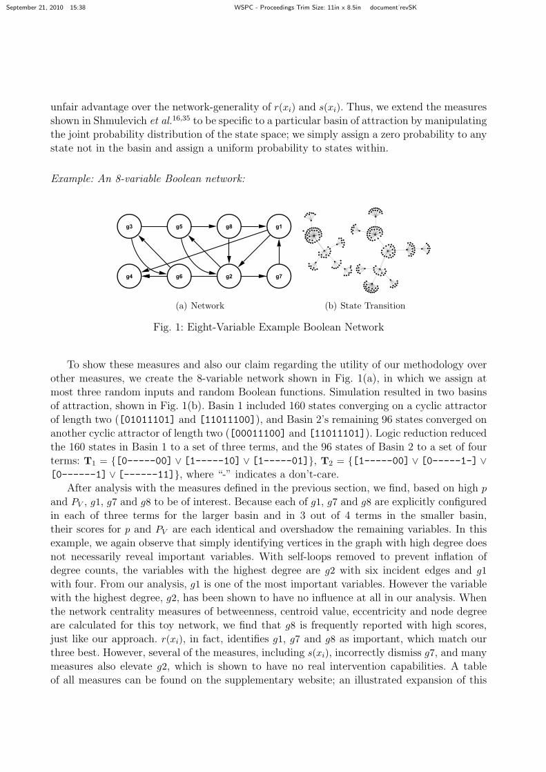
Example: An 8-variable Boolean network:

(a) Network (b) State Transition

Fig. 1: Eight-Variable Example Boolean Network

To show these measures and also our claim regarding the utility of our methodology overother measures, we create the 8-variable network shown in Fig. 1(a), in which we assign atmost three random inputs and random Boolean functions. Simulation resulted in two basinsof attraction, shown in Fig. 1(b). Basin 1 included 160 states converging on a cyclic attractorof length two ([01011101] and [11011100]), and Basin 2’s remaining 96 states converged onanother cyclic attractor of length two ([00011100] and [11011101]). Logic reduction reducedthe 160 states in Basin 1 to a set of three terms, and the 96 states of Basin 2 to a set of fourterms: T1 = {[0-----00] ∨ [1-----10] ∨ [1-----01]}, T2 = {[1-----00] ∨ [0-----1-] ∨[0------1] ∨ [------11]}, where “-” indicates a don’t-care.

After analysis with the measures defined in the previous section, we find, based on high p

and PV , g1, g7 and g8 to be of interest. Because each of g1, g7 and g8 are explicitly configuredin each of three terms for the larger basin and in 3 out of 4 terms in the smaller basin,their scores for p and PV are each identical and overshadow the remaining variables. In thisexample, we again observe that simply identifying vertices in the graph with high degree doesnot necessarily reveal important variables. With self-loops removed to prevent inflation ofdegree counts, the variables with the highest degree are g2 with six incident edges and g1

with four. From our analysis, g1 is one of the most important variables. However the variablewith the highest degree, g2, has been shown to have no influence at all in our analysis. Whenthe network centrality measures of betweenness, centroid value, eccentricity and node degreeare calculated for this toy network, we find that g8 is frequently reported with high scores,just like our approach. r(xi), in fact, identifies g1, g7 and g8 as important, which match ourthree best. However, several of the measures, including s(xi), incorrectly dismiss g7, and manymeasures also elevate g2, which is shown to have no real intervention capabilities. A tableof all measures can be found on the supplementary website; an illustrated expansion of this


example, along with a simpler one, can be also be found there, and in our previous report.29

4. Results

In this section we set out to prove the efficacy of our method on real world examples. For thisproof of concept we analyze a Boolean network model of the yeast cell cycle and identify sig-nificant variables in the system corroborated by its original manuscript. We then demonstrateour approach on a Boolean network not constructed manually, but rather learned from geneexpression data directly. In our technical report29 we also apply our method to the systemsbiology of human aging, where we step away from genetic interactions and demonstrate theutility of our method on our Boolean network model for human senescence.

4.1. Boolean Network Model for Yeast Cell Cycle and Its Analysis

As a proof of concept on a nonrandom network we will apply our methodology to a well-studied Boolean network model of the yeast cell cycle5 and show that key variables describedin the manuscript are identified by our approach. In their paper, Li et al. manually construct aBoolean network modeling the yeast cell cycle using 11 of the most important genes out of theapproximately 800 known to play a role in the process. This network is simulated and resultsin seven basins of attraction, one of which is by far the largest and was studied exclusively inthe paper. In this basin of attraction, which included 1,764 states, Li et al. were able to tracethe trajectory of the yeast cell cycle from one of the fringe, or “Garden of Eden”,4 states downto the eventual point attractor state. The Boolean network adapted from Li et al. is shown inon the supplementary website, the original paper,5 and our technical report.29

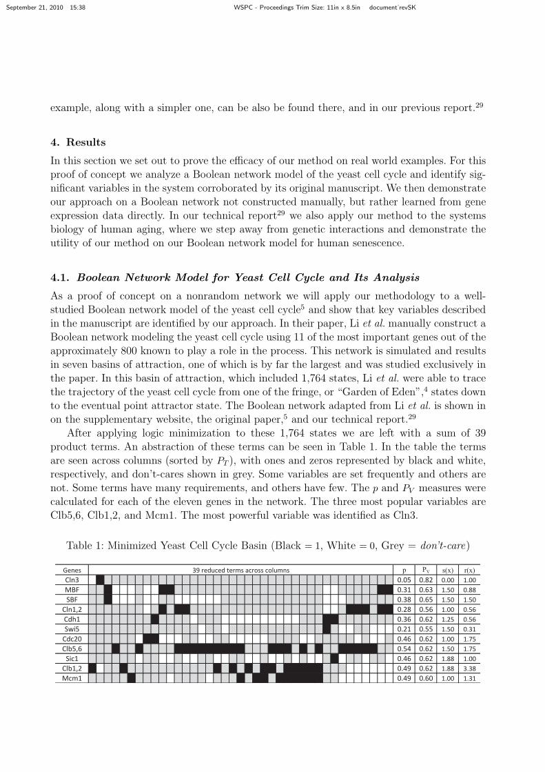
After applying logic minimization to these 1,764 states we are left with a sum of 39product terms. An abstraction of these terms can be seen in Table 1. In the table the termsare seen across columns (sorted by PT ), with ones and zeros represented by black and white,respectively, and don’t-cares shown in grey. Some variables are set frequently and others arenot. Some terms have many requirements, and others have few. The p and PV measures werecalculated for each of the eleven genes in the network. The three most popular variables areClb5,6, Clb1,2, and Mcm1. The most powerful variable was identified as Cln3.

Table 1: Minimized Yeast Cell Cycle Basin (Black = 1, White = 0, Grey = don’t-care)

Genes p PV s(x) r(x)

Cln3 0.05 0.82 0.00 1.00

MBF 0.31 0.63 1.50 0.88

SBF 0.38 0.65 1.50 1.50

Cln1,2 0.28 0.56 1.00 0.56

Cdh1 0.36 0.62 1.25 0.56

Swi5 0.21 0.55 1.50 0.31

Cdc20 0.46 0.62 1.00 1.75

Clb5,6 0.54 0.62 1.50 1.75

Sic1 0.46 0.62 1.88 1.00

Clb1,2 0.49 0.62 1.88 3.38

Mcm1 0.49 0.60 1.00 1.31

39 reduced terms across columns


Starting with the most popular variable, we find that Clb5,6 is required to be in a particularstate 54 percent of the time. Furthermore we find that in each of the 21 terms in which Clb5,6is in a specific configuration, that configuration is ON, or active. Since the Clb5 gene (part ofthe Clb5,6 variable) is described as being responsible for driving the cell into the S phase (inwhich the DNA is synthesized and chromosomes are replicated), it seems reasonable to find itstrongly represented in the minimized basin. If the role of Clb5 were not known beforehand,analysis of the basin in the manner described could identify it as important (and in the ONstate) even though it is OFF in the eventual attractor state.

Next we look at one of the second-most popular variables in the reduced basin, namelyClb1,2. The Clb2 gene (part of the Clb1,2 variable) is stated as being responsible for the tran-sition in and out of the M phase (in which chromosomes are separated and the cell is dividedinto two). Thus, like Clb5,6, it is not surprising to find it here among the most frequentlyspecified variables in the basin representing the cell cycle. Unlike Clb5,6, the configuration ofClb1,2 is not consistent—it is found in the OFF configuration 7 times and in the ON configu-ration 12 times. However, since it is the activation and subsequent degradation of Clb2 whichinitiates and terminates the M phase, the split nature of the configurations seems appropriate.

There are other variables with high p which are not explicitly called out in the paper.Given the corroboration of those which are called out in the paper, further investigation ofthe roles of cyclin inhibitors Cdc20 and Sic1, and of transcription factor Mcm1 is warranted.

Finally we look at the most powerful variable, cyclin Cln3, which was described in thepaper as the trigger committing the cell to the division process. Despite its importance, wefind it only explicitly configured in 2 of the 39 terms in the reduced basin (once for OFFand once for ON ), which ranks it lowest in the p measure. However, because these two termsare the most powerful, Cln3’s PV score is quickly elevated. It is also interesting to find thatin these two terms, only one other variable is specifically configured, namely, Clb1,2. In fact,these two variables are in opposite configurations in these two terms; when Cln3 is ON, Clb1,2is OFF and when Cln3 is OFF, Clb1,2 is ON. This is interesting because Cln3 is described astriggering the G1 phase (the starting phase), and Clb1,2 controls the entry and exit from theM phase (the ending phase). Their opposite configurations in the reduced basin terms seemto agree quite harmoniously with their regulatory control at extreme ends of the cell cycle.

When the network centrality measures of betweenness, centroid value, eccentricity andnode degree are calculated for this yeast network, we find that Clb1,2 and Clb5,6 are frequentlyreported with high scores, just like we find using our approach. This is also the case whenr(xi) is calculated based on the Boolean network properties underlying the topology. However,the centrality measures also report variables such as Clb1,2, SBF and MBF, which are shownmathematically by our method to have little intervention power. Furthermore, these measuresgive little consideration to other key variables, including Cln3 and Mcm1, which our approachmathematically shows to have some intervention capabilities. Thus, our approach reports thekey variables described by Li et al. and missed by traditional measures, and avoids reportingmathematically weak variables reported strongly by traditional measures.


4.2. Application to WNT5A Network for Melanoma

After applying our approach to a hand-made network, we applied our methodology to a well-studied WNT5A network computationally predicted from a melanoma data set.36–38 In ourprevious work,38 the original data set was narrowed down to the ten most critical variables;these were selected out of 587 total on the basis of their strong interactive connectivity andeither their known or likely roles in WNT5A driven induction of an invasive phenotype inmelanoma cells, or their close predictive relationship with these genes. For each of the tenvariables, we were able to identify the three most ideal predictors out of the remaining nine.Using this connectivity and a binary quantization of the original data set, the best binary logicfunctions were inferred for each target minimizing the Bayes error.39,40 From these functions,the Boolean network attractors and basins were identified. The reader is referred to the citedpublications for detailed information on the data and connectivity, and to the supplementarywebsite for the functions identified, as well as elucidating figures.

Table 2: WNT5A Basin Attractor States (Black = 1, White = 0) with Basin Measures; si(x)and ri(x) are basin-specific influence and sensitivity, which are discussed in the next subsection

B1 p PV s1(x) r1(x) p PV s2(x) r2(x) B3 p PV s3(x) r3(x) s(x) r(x)

WNT5A 0.45 0.57 1.79 2.25 0.70 0.44 1.72 1.70 1.00 0.20 1.00 2.75 1.75 2.00

S100B 0.32 0.53 1.03 0.88 0.40 0.40 0.96 0.59 1.00 0.20 1.25 1.25 1.00 0.75

RET1 0.23 0.54 0.00 1.22 0.35 0.46 0.00 1.29 0.50 0.20 0.00 1.00 0.00 1.25

MMP-3 0.50 0.55 0.00 0.51 0.60 0.48 0.00 0.47 1.00 0.20 0.00 1.00 0.00 0.50

Pho-C 0.27 0.53 0.96 0.24 0.35 0.37 0.52 0.27 0.50 0.20 0.50 0.00 0.75 0.25

MLANA 0.00 0.00 1.26 0.90 0.00 0.00 1.24 0.58 0.00 0.00 1.00 1.00 1.25 0.75

HADHB 0.32 0.50 0.81 0.74 0.55 0.41 0.64 0.77 1.00 0.20 3.00 0.50 0.75 0.75

SNCA 0.68 0.54 1.65 0.30 0.70 0.50 1.31 0.19 1.00 0.20 2.50 0.25 1.50 0.25

STC2 0.82 0.55 1.31 1.08 0.75 0.47 1.19 0.92 1.00 0.20 1.00 0.25 1.25 1.00

PIR 0.86 0.55 1.79 2.48 0.70 0.49 1.71 2.51 1.00 0.20 1.00 3.25 1.75 2.50

B2

The state space (1,024 states) was partitioned into three basins of attraction: Basin 1 hada singleton attractor state with a total basin size of 544 states, Basin 2 has a two-state cyclicattractor with a total basin size of 472 states, and Basin 3 had a singleton attractor witha total basin size of just 8 states. As seen in Table 2, our measures p and PV reported theintervention capabilities of Pirin, STC2, SNCA, and WNT5A. STC2 is known to interact withMMP-3,41 another variable in this network, SNCA is known to be aberrantly hypermethylatedin human cancer cells,42 it is known that “cytoplasmic localization of PIR may represent acharacteristic of WNT5A network for melanoma progression”,43 and WNT5A has a knownrole in human melanoma progression.37 That three of our top four intervention targets areeither melanoma-related or cancer-related speaks well for their true intervention capabilities.

When compared to the network centrality measures, as well as r(xi) and s(xi), Pirin andWNT5A were identified by most of them. However, also among the high scoring results forthese measures was MLANA, which was shown mathematically by our results to have zeroinfluence on the network dynamics. This is not totally surprising, considering this network is


derived from melanoma data in which all melanocytes should be present, and that p and PV arebasin-specific (see below). While all variables in such a small, carefully selected set will bearsome significance, even MLANA, our approach simply reveals those with true interventioncapabilities given the topology. Furthermore, some measures dismissed STC2 and SNCA byincluding it among the lowest scoring variables despite its influence potential.

4.3. Usefulness of p and PV over Other Measures

We have seen the ability of p and PV to identify variables with great combinatorial controlover the state space of a Boolean network. We have further demonstrated how those variablesidentified are often known to be suitable targets for intervention. In demonstrating this wehave compared p and PV to r(xi) and s(xi), as well as network centrality measures, and herewe discuss some differences in these measures.

While r(xi) and s(xi) are based on Boolean functions, p and PV are based on Boolean states.Influence16 is computed by variable pairs in a matrix and summed by rows and columns toget r(xi) and s(xi), where p and PV are independent measurements on variables and do notdepend on pairs. r(xi) and s(xi) are general measures, where p and PV are specific to eachbasin of attraction. To level the field of comparison, we created a basin-specific version ofr(xi) and s(xi) (rk(xi) and sk(xi) for basin k), but they were not able to offer any new insightthat r(xi) and s(xi) were not already able to. To see this, observe the closeness and value andsymmetry in dynamics (based on basin size) between the measurements in Table 2 and in thetable on the supplementary website for the human aging network.

There are additional advantages over r(xi) and s(xi). p and PV are not only basin-specific,but they are also value-specific. While we can adapt an influence matrix to be basin-specific, itstill cannot be made value-specific. Thus, with p and PV , because of the minimized terms, wenot only know where to intervene, but precisely how to do so. These values, or how we shouldintervene, can be and often are different than the values in the attractor state (if we’re luckyenough to not have a cyclic attractor where values toggle), and furthermore the same targetmay be viable for more than one basin, but with different values. This kind of information isnot available with an influence matrix or the derived measures r(xi) and s(xi).

Furthermore, p and PV allow us to find the minimal effective intervention. Any computa-tional aid to intervention studies will always be human-reviewed in the end, so it need notgive one definitive answer. We can say with mathematical certainty that setting certain vari-ables together will force a basin (and thus attractor) to be selected. With a set of minimizedterms we can find the smallest interventions (highest PT ) using the most effective targets(high p and/or PV ) which are suitable for intervention with current medical abilities (humanevaluation of mathematical possibilities).

5. Conclusion and Future Work

In this paper, we showed the importance of analyzing Boolean network basins of attractionin identifying targets for intervention. Furthermore, we demonstrated that these targets arenot always evident in attractor states themselves, in the network topology, or even fromvarious existing measures, both graph-theoretic and Boolean-network-specific. Our use of logic


minimization significantly reduces the representation of basins of attraction, and the proposedmeasures stratify the terms, revealing both the key players and how to manipulate them.

The analysis of the yeast cell cycle network demonstrated that our methodology can iden-tify key variables in the system. We were able to systematically identify three importantvariables described specifically by the original study and propose others for further study. Ourapplication to the WNT5A network for melanoma demonstrated the applicability of our ap-proach beyond hand-created networks to networks inferred from biological data; furthermoreour targets identified for intervention had been previously validated by laboratory studies.

This approach is most appropriate to smaller hand-made or high-confidence networksdue to the size complexity issues in Boolean networks. Current efforts involve overcomingthe scalability issues inherent in enumerating complete state spaces, which quickly becomesintractable. We are investigating approximation approaches to identify attractor states andenumerate most of their basins. We intend to take full advantage of high performance comput-ing clusters, both in terms of memory and parallelization. We also are working on expandingour implementations and measures to handle multi-valued logic, taking us beyond the Booleanconstraint and allowing even more levels of abstraction.

Supplementary Material

http://biocomputing.asu.edu/basinreduction/psb2011/

Acknowledgement

This study funded partly by NIH R21LM009706 (MV, SK) and SFAZ CAA 0243-08 (SK).

References

1. J. Goutsias and S. Kim, Biophys J 86, 1922 (April 2004).2. S. Kauffman, Journal of Theoretical Biology 22, 437 (March 1969).3. G. Lima-Mendez and J. Helden, Mol. BioSyst. 5, 1482 (December 2009).4. A. Wuensche, Genomic regulation modeled as a network with basins of attraction., in Pacific

Symposium on Biocomputing , 1998.5. F. Li, T. Long, Y. Lu, Q. Ouyang and C. Tang, Proceedings of the National Academy of Sciences

of the United States of America 101, 4781 (April 2004).6. R. Albert and H. G. Othmer, Journal of Theoretical Biology 223, 1 (July 2003).7. J. Yu, V. A. Smith, P. P. Wang, A. J. Hartemink and E. D. Jarvis, Bioinformatics 20, bth448

(July 2004).8. V. A. Smith, E. D. Jarvis and A. J. Hartemink, Bioinformatics 18, S216 (July 2002).9. C. Gershenson, Classification of random boolean networks, in ICAL 2003: Proceedings of the

eighth international conference on Artificial life, (MIT Press, Cambridge, MA, USA, 2003).10. K. Klemm and S. Bornholdt, Physical Review E 72, 055101+ (Nov 2005).11. F. Greil and B. Drossel, Physical Review Letters 95, 048701+ (Jul 2005).12. X. Deng, H. Geng and M. Matache, Biosystems 88, 16 (March 2007).13. T. Akutsu, S. Miyano and S. Kuhara, Pacific Symposium on Biocomputing , 17 (1999).14. I. Shmulevich, A. Saarinen, O. Yli-Harja and J. Astola, Inference of genetic regulatory networks

via best-fit extensions, in Computational and Statistical Approaches to Genomics, eds. W. Zhangand I. Shmulevich (Kluwer Academic Publishers, Boston, 2003) pp. 197–210.


15. H. Lahdesmaki, I. Shmulevich and O. Yli-Harja, Machine Learning 52, 147 (July 2003).16. I. Shmulevich, E. R. Dougherty, S. Kim and W. Zhang, Bioinformatics 18, 261 (February 2002).17. A. Datta, A. Choudhary, M. L. Bittner and E. R. Dougherty, Machine Learning 52, 169 (July

2003).18. A. Datta, A. Choudhary, M. L. Bittner and E. R. Dougherty, Bioinformatics 20, 924 (April

2004).19. R. Pal, A. Datta, M. L. Bittner and E. R. Dougherty, Bioinformatics 21, 1211 (April 2005).20. A. Choudhary, A. Datta, M. L. Bittner and E. R. Dougherty, Bioinformatics 22, 226 (January

2006).21. K. A. Richardson, Advances in Complex Systems 8, 365 (2005).22. E. Dubrova, M. Teslenko and H. Tenhunen, A computational scheme based on random boolean

networks, in Transactions on Computational Systems Biology X , eds. C. Priami, F. Dressler,O. B. Akan and A. Ngom, 2008) pp. 41–58.

23. J. Saez-Rodriguez, L. G. Alexopoulos, J. Epperlein, R. Samaga, D. A. Lauffenburger, S. Klamtand P. K. Sorger, Molecular Systems Biology 5 (December 2009).

24. R. Schlatter, K. Schmich, I. Avalos Vizcarra, P. Scheurich, T. Sauter, C. Borner, M. Ederer,I. Merfort and O. Sawodny, PLoS Comput Biol 5, e1000595+ (December 2009).

25. L. J. Steggles, R. Banks, O. Shaw and A. Wipat, Bioinformatics 23, 336 (February 2007).26. P. Maji, Fundam. Inf. 86, 143 (2008).27. J. C. Mar and J. Quackenbush, PLoS Comput Biol 5, e1000626+ (December 2009).28. D. Bryce, M. P. Verdicchio and S. Kim, ACM Transactions on Intelligent Systems and Technology

(To Appear).29. M. P. Verdicchio and S. Kim, Reduction of Boolean Network Basins of Attraction Reveals Inter-

vention Targets, tech. rep., Arizona State University (Tempe, AZ, 2010).30. Y. Xiao, Current Genomics 10, 511 (November 2009).31. I. Shmulevich, E. R. Dougherty and W. Zhang, Bioinformatics 18, 1319 (October 2002).32. A. Marcovitz, Introduction to Logic Design, first edn. (McGraw-Hill, Feb 2002).33. R. L. Rudell and A. L. Sangiovanni-Vincentelli, Espresso-mv: Algorithms for multiple valued

logic minimization, in Proc. of the IEEE Custom Integrated Circuits Conference, 1985.34. G. Scardoni, M. Petterlini and C. Laudanna, Bioinformatics 25, 2857 (November 2009).35. I. Shmulevich and S. A. Kauffman, Physical Review Letters 93, 048701+ (Jul 2004).36. M. Bittner, P. Meltzer, Y. Chen, Y. Jiang, E. Seftor, M. Hendrix, M. Radmacher, R. Simon,

Z. Yakhini, A. Ben-Dor, N. Sampas, E. Dougherty, E. Wang, F. Marincola, C. Gooden, J. Lueders,A. Glatfelter, P. Pollock, J. Carpten, E. Gillanders, D. Leja, K. Dietrich, C. Beaudry, M. Berens,D. Alberts and V. Sondak, Nature 406, 536 (August 2000).

37. A. T. Weeraratna, Y. Jiang, G. Hostetter, K. Rosenblatt, P. Duray, M. Bittner and J. M. Trent,Cancer Cell 1, 279 (April 2002).

38. S. Kim, H. Li, E. R. Dougherty, N. Cao, Y. Chen, M. Bittner and E. B. Suh, Journal of BiologicalSystems 10, 337 (2002).

39. E. R. Dougherty, S. Kim and Y. Chen, Signal Processing 80, 2219 (2000).40. S. Kim, E. R. Dougherty, M. L. Bittner, Y. Chen, K. Sivakumar, P. Meltzer and J. M. Trent,

Journal of biomedical optics 5, 411 (October 2000).41. J. Y. Y. Sung, S. M. M. Park, C.-H. H. Lee, J. W. W. Um, H. J. J. Lee, J. Kim, Y. J. Oh,

S.-T. T. Lee, S. R. Paik and K. C. C. Chung, The Journal of biological chemistry 280, 25216(July 2005).

42. A. Y. Law, K. P. Lai, C. K. Ip, A. S. Wong, G. F. Wagner and C. K. Wong, Experimental cellresearch 314, 1823 (May 2008).

43. S. Licciulli, C. Luise, A. Zanardi, L. Giorgetti, G. Viale, L. Lanfrancone, R. Carbone and M. Al-calay, BMC cell biology 11, 5+ (January 2010).

IDENTIFYING TARGETS FOR INTERVENTION BY ANALYZING … · September 21, 2010 15:38 WSPC -...

Documents

Transcript of IDENTIFYING TARGETS FOR INTERVENTION BY ANALYZING … · September 21, 2010 15:38 WSPC -...