
Identifying Fixed Export Costs and their Impact on Firm .... Castro_ExportCosts.… · Comments...
47
Identifying Fixed Export Costs and their Impact on Firm-Level Export Behavior ∗ Luis Castro † Ben Li ‡ Keith E. Maskus § Yiqing Xie ¶ This draft: August 15, 2012 Comments welcome Abstract The literature on trade and firm heterogeneity emphasizes two parameters that affect firm- level export decisions: productivity and fixed trade costs. The importance of productivity has been extensively documented in empirical studies, whereas much less is known about the empir- ical relevance of fixed trade costs and how the two parameters interact with each other. Using total export expenses collected by the Annual National Industrial Survey of Chile, we estimate a schedule of fixed trade costs for all industries, regions, and years in Chile, which helps to pin- point the fixed trade costs that any firm would pay if it wants to export. Based on this schedule, we reach three findings. First, fixed trade costs discourage exports. Other factors held constant, a change in fixed trade costs from the 25th percentile to the 75th percentile of the schedule reduces export propensity by approximately 5%. Second, given the same export propensity, higher productivity and lower fixed trade costs are substitutable, and the substitution becomes weaker as productivity rises. Third, high-productivity non-exporters are associated with high fixed trade costs. ∗ The paper used to circulated under the title “Heterogeneous Fixed Trade Cost and Firm-level Exporting Per- formance.” We thank Mary Amiti, James Anderson, Daniel Bernhofen, David Hummels, Beata Javorcik, Wolfgang Keller, Edwin Lai, Peter Neary, James Tybout, Zhihong Yu, and the audiences at Boston College, University of Oxford, Nottingham University, Stockholm University, Ljubljana Empirical Trade Conference, Midwest International Economics Group, and Bolivian Conference on Development Economics for their valuable comments. We particu- larly thank Jagadeesh Sivadasan who provides us with the stata routine that implements the Ackerberg-Caves-Frazer (2006) method. All remaining errors are ours. † Department of Economics, University of Colorado at Boulder, email: [email protected]. ‡ Department of Economics, Boston College, email: [email protected]. § Department of Economics, University of Colorado at Boulder, email: [email protected]. ¶ Department of Economics, University of North Dakota, email: [email protected].
Transcript of Identifying Fixed Export Costs and their Impact on Firm .... Castro_ExportCosts.… · Comments...

Identifying Fixed Export Costs and their Impact onFirm-Level Export Behavior∗
Luis Castro† Ben Li‡ Keith E. Maskus§ Yiqing Xie¶
This draft: August 15, 2012Comments welcome
Abstract
The literature on trade and firm heterogeneity emphasizes two parameters that affect firm-level export decisions: productivity and fixed trade costs. The importance of productivity hasbeen extensively documented in empirical studies, whereas much less is known about the empir-ical relevance of fixed trade costs and how the two parameters interact with each other. Usingtotal export expenses collected by the Annual National Industrial Survey of Chile, we estimatea schedule of fixed trade costs for all industries, regions, and years in Chile, which helps to pin-point the fixed trade costs that any firm would pay if it wants to export. Based on this schedule,we reach three findings. First, fixed trade costs discourage exports. Other factors held constant,a change in fixed trade costs from the 25th percentile to the 75th percentile of the schedulereduces export propensity by approximately 5%. Second, given the same export propensity,higher productivity and lower fixed trade costs are substitutable, and the substitution becomesweaker as productivity rises. Third, high-productivity non-exporters are associated with highfixed trade costs.
∗The paper used to circulated under the title “Heterogeneous Fixed Trade Cost and Firm-level Exporting Per-formance.” We thank Mary Amiti, James Anderson, Daniel Bernhofen, David Hummels, Beata Javorcik, WolfgangKeller, Edwin Lai, Peter Neary, James Tybout, Zhihong Yu, and the audiences at Boston College, University ofOxford, Nottingham University, Stockholm University, Ljubljana Empirical Trade Conference, Midwest InternationalEconomics Group, and Bolivian Conference on Development Economics for their valuable comments. We particu-larly thank Jagadeesh Sivadasan who provides us with the stata routine that implements the Ackerberg-Caves-Frazer(2006) method. All remaining errors are ours.
†Department of Economics, University of Colorado at Boulder, email: [email protected].‡Department of Economics, Boston College, email: [email protected].§Department of Economics, University of Colorado at Boulder, email: [email protected].¶Department of Economics, University of North Dakota, email: [email protected].

1 Introduction
Over the past decade, a phenomenal innovation in the trade theory was the introduction of firm-level export decisions. The key idea can be summarized using a sorting mechanism based onproductivity and fixed export costs: a fixed export cost has to be paid if a firm exports, suchthat only firms that can garner enough profits choose to pay that cost and export.1 Two logicalimplications follow: (1) given fixed export costs, firms with high productivity export, and (2) givenproductivity, firms with low fixed export costs export. There has been extensive empirical evidenceon the productivity premium of exporters relative to nonexporters;2 however, a direct test of (1)and (2) remains absent due to the empirical challenge in measuring fixed export costs: nonexportersdo not pay fixed export costs such that their fixed export costs are counter-factual.
The existing literature assumes a homogeneous fixed export cost for all firms, under whichthe productivity premium of exporters is sufficient to establish the sorting mechanism. Comparedto productivity that varies by firm, fixed export costs are likely more homogeneous. Regardless,homogeneous fixed export costs across firms all over an economy (e.g., a country) is too strong anassumption. Furthermore, assuming homogeneous fixed export costs makes the test of the sortingmechanism less conclusive, because the productivity premium of exporters, even if being the keydifference between exporters and nonexporters, can be linked to various causes that select onlysome firms as exporters. For example, exporters with high productivity (i.e., with low variableproduction costs) may also perform better designing, marketing, and distribution that give themthe edge in foreign markets.
In this paper, we use firm-level export expenses reported by the Annual National IndustrialSurvey of Chile (Encuesta Nacional Industrial Anual, or ENIA), to construct industry-region-yeartuple level indices of fixed export costs. Then, we empirically examine how firms’ export decisionsvary with productivity as well as the fixed export costs of the tuples in which they locate. Ourexamination leads to three findings. The primary finding is that, with productivity held constant,high fixed export costs are associated with a low export propensity. Moving from the 25th to the75th percentile of the fixed export cost index, export propensity lowers by approximately 6 to 12percent. In particular, high-productivity nonexporters face high fixed export costs.
******** Figure 1 about here ********
A graphical illustration of this is provided in Figure 1 for two largest industries in our dataset,“fabricated metal” (upper) and “wood and cork” (lower), where high (low) productivity is definedas equally or more (less) productive than the 75th percentile exporter. We compare the fixedexport costs, measured by three indices that are discussed later, of high-productivity nonexporterswith those of low-productivity exporters and report t-statistics in the upper-right corners of the
1See e.g., Helpman, Melitz, and Yeaple (2004), Melitz (2003), and Yeaple (2005).2For discussions on the econometric estimation of firm productivity, see Ackerberg, Caves, and Frazer (2006),
Levinsohn and Petrin (2003), and Olley and Pakes (1996). For discussions on the productivity premium of exporters,see Bernard and Jensen (1999, 2004), De Loecker (2007), and Lileeva and Trefler (2009).
2
two panels. All the differences are significant at least at the 5% level. This explains a well-documented puzzling productivity overlap in the data:3 some nonexporters are more productivethan some exporters. To explain this puzzle, a usual instinct resorts to factors outside the sorting-by-productivity theory, though this theory has provided an answer so along as differences in fixedexport costs are considered.
Given the first and primary finding, the other two follow naturally. For one, given the sameexport propensity, high productivity and low fixed export costs are substitutable; further, thissubstitution effect is decreasing in firm-level productivity. That is, covering fixed export costs isless a concern for high-productivity firms than for low-productivity ones when they make exportdecisions. For two, at the tuple level, the export volume of an average exporter is larger whereeither fixed export costs or productivity dispersion is larger, because high fixed export costs raisethe productivity threshold for exporting, while a larger despersion of productivity engenders morefirms that reach the threshold. In either case, the average firms that end up exporting are moreproductive.
One important feature of this paper is its reduced-form approach. Since the ENIA providesdata on exporters’ export expenses, we have the variation in export costs in addition to variationsin export decisions and productivity. We estimate the fixed component in export expenses, namelythe expenses that do not vary by export volume, and use it along with the information on exportdecisions and productivity. The three pieces of information together enable us to examine exportdecisions conditional on fixed export costs and productivity. This departs from the empiricalliterature which, with the variation in export costs absent, uses export decisions to infer fixedexport costs.4 This literature usually assumes concrete profit functions and demand systems, andthen structurally estimates or calibrates the parameters of fixed export costs at various levels (e.g.,firm, industry, destination country, and country). With this approach, export behaviors and fixedexport costs are essentially two flipsides of one coin, because they stem from the same variation inthe data.
The limitation of this paper is that it draws little light on the sunk costs paid by firms to startexporting. The fixed export cost indices in this paper are constructed using the export expensespaid by exporters, which are necessary for nonexporters if they decided to export, but perhapsinsufficient. Nonexporters may need to pay additional costs for preliminary credentials in theexporting business, usually referred to as sunk export costs in the literature. This paper addressesthe counter-factuality of fixed export costs faced by nonexporters, but not that of sunk export costs.Sunk export costs are estimable with structures that assume how they spread over exporters’ lifecourse,5 and the silence on this is a cost for us to use a reduced-form approach.6
3See, e.g., Bernard, Eaton, Jensen, and Kortum (2003, US firms), Mayer and Ottaviano (2008, Belgian firms),Wakasugi (2009, Japanese firms). We find the same pattern in Chilean firms (see Figure 1).
4See Arkolakis (2010), Das, Roberts, and Tybout (2007), Eaton, Kortum, and Kramarz (2011), Hanson and Xiang(2011), Irarrazabal, Moxnes, and Opromolla (2010), and Roberts and Tybout (1997). Among them, Hanson andXiang (2011) is an exception that uses reduced-form estimation on separable variations in the data, but their focusis different from ours; they focus on the importance of global relative to bilateral fixed export costs.
5For example, Das, Roberts, and Tybout (2007) and Roberts, and Tybout (1997).6Sunk costs may also be estimable using a reduced-form approach if there are a large number of firms that change
3

Apart from key evidence of the sorting-by-productivity mechanism, this paper also speaks to theliterature on trade costs. This literature has mostly focused on variable trade costs.7 This paperdocuments a positive association between average export volume of exporters and fixed exportcosts as well as productivity dispersion, indicating that fixed export costs change the composition ofexporters. This said, a data-based measure of fixed export costs will be a linchpin to understandinghow micro-level exports aggregate into industry and country trade statistics.
The rest of the paper is organized as follows. Section 2 builds a theoretical framework andpresents its predictions. Section 3 discusses data and the construction of fixed export cost indices.Section 4 reports our empirical findings. Section 5 concludes.
2 Conceptual framework
This section employs a simple theoretical model to generate testable predictions.8 Consider twocountries, Home and Foreign (rest of the world). They have the same preference over a collectionof varieties made in Home:9
U =
ˆj∈J
x(j)αdj
1α
,
where j is the variety index, J is the set of varieties, and 0 < α < 1 determines the elasticity ofsubstitution between varieties σ ≡ 1/(1 − α). The foreign demand for a particular variety j madein Home i
x(j) = p(j)−σγ
P 1−σ, (1)
where p(j) is delivery price,
P ≡
ˆj∈J
p(j)1−σdj
1/(1−σ)
(2)
is the foreign price index associated with imported varieties J , and γ is the foreign expenditurespent on imported varieties.
In Home, each variety j is produced by a unique firm, labeled as firm j. The factor demandper unit output of firm j is denoted by a(j). Firms compete in a monopolistic competition fashion
their export statuses, which is however not our case. Appendix A1 lists the number and share of firms that changetheir export statuses in our sample. They are overall rare and moreover usually firms that frequently switch betweenexport statuses.
7See Anderson and van Wincoop (2003, 2004), Anderson and Yotov (2008), Bernard, Jensen, and Schott (2006),Bougheas, Demetriades, and Morgenroth (1999), Blonigen and Wilson (2008), Clark, Dollar, and Micco (2004),Donaldson (2010), Limão and Venables (2001), Wilson, Mann, and Otsuki (2003), among others. Helpman, Melitz,and Rubinstein (2008) introduce fixed export costs to the studies on aggregate trade statistics, but takes it as aconfounding factor to control for.
8It is a variant of Melitz (2003) and Helpman, Melitz and Rubinstein (2008).9This is only part of the utility function. The utility from consuming varieties made in Foreign is not relevant to
our context, so we do not write it out.
4

in the foreign market, leading to constant mark-up pricing:
p(j) = va(j)cα
, (3)
where v > 1 is an iceberg variable trade cost and c is the factor price. Combining equations (1)with (3), we obtain firm j’s potential profit from exporting:
π(j) = χa(j)1−σ − f, (4)
where χ ≡ (1−α)(τc/αP )1−σγ, and f is the fixed export cost. Since productivity is inversely relatedto unit factor demand, we define A ≡ a1−σ, a decreasing function of a, to denote productivity. Whenconfusion does not arise, we suppress the index j.
Next, define X(j) as export indicator, a binary variable that denotes whether firm j exports,and Pr(X(j) = 1) as export propensity of firm j. Export propensity depends on the potential profitfrom exporting π(j):
Pr[X(j) = 1] = Ψ[π(j)], (5)
where Ψ is a function: if π < 1, Ψ[π] = 0; if π ≥ 1, Ψ[π] > 0. Here, 1 can be considered asthe smallest unit of currency or a uniformly applied lump-sum tax, which will prove useful later.Equation (5) implies that firm j does not export if its potential profit is negative or very close tozero. The economics underpinning equation (5) is as follows. To serve the foreign market, eachexporter has to draw a foreign client (e.g., an importer) with parameter u to work with, and thisrelationship works out only if π(j) > u. This u can be thought of the minimum caliber the foreignclient requires. u follows distribution Φ(u) with a decreasing density when u > 0; that is, thecaliber requirements are concentrated in low values.
In the following, we assume Φ(u) to be a standard normal distribution, such that Ψ′[π] > 0 andΨ′′[π] < 0 if π ≥ 1,10 and moreover equation (5) directly translates to a probit model that we uselater.11,12 That is, if firm j’s expected profit from exporting is greater than 1, its export propensityincreases in the expected profit, while the increase is less than proportional. Intuitively, firmswith higher π’s have higher export propensities because they are easier to find a match client, butincreasing π does not improve export propensity proportionally, because clients that require veryhigh calibers are small in number. Also, for later use, we define A∗ such that π(j) = χA∗ − f = 1;clearly, A∗ is an increasing function of f .
Since our focus is on the foreign market, we assume for simplicity that all firms serve the home10Notice that 1 is the inflection point of the probability density function of a standard normal distribution.11Notably, if Φ(u) follows distribution N(0, ∆2) with ∆ > 0, ∆ = 1, i.e., a normal but not standard normal
distribution, ∆ cannot be identified separately from the coefficients in a probit model.12Formally,
Pr[X(j) = 1] = Ψ[π] ={
Pr[π ≥ u] = Φ[π], if π ≥ 1,
0, if π < 1.
In the upper case, Ψ′[π] = Φ′[π] = ϕ[π] > 0, Ψ′′[π] = Φ′′[π] = ϕ′[π] < 0. Note that a standard probit model usesπ = 0 rather than π = 1 as the threshold but 1 will be absorbed by the constant term of the probit model.
5

market and the total number of home firms is constant.13 The game of exporting works as follows.Firms draw A from G(A), f from Γ(f), and u from Φ(u); then their export decisions are madeaccording to equations (4) and (5). We now move on to the three empirical implications of themodel that will be tested later.
Hypothesis I (export propensity) The export propensity of firms is decreasing in the fixed ex-port cost f .
This prediction follows straightforward given d Pr(X=1)df = Ψ′[π]∂π
∂f = −Ψ′[π] ≤ 0; the inequality isstrict when π ≥ 1. Hypothesis I has another version that focuses on high-productivity nonexporters.Since firms with π < 1 do not export, E(π|X = 1) > E(π|X = 0); therefore,
E(χA|X = 1) − E(f |X = 1) > E(χA|X = 0) − E(f |X = 0), (6)
orE(f |X = 0) − E(f |X = 1) > E(χA|X = 0) − E(χA|X = 1). (7)
When the right side of inequality (7) is positive, the left side must be positive. That is, if somenonexporters are more productive than some exporters, they are expected to be associated withhigher fixed export cost than the exporters. If we call these nonexporters and exporters as high-productivity nonexporters and low-productivity exporters, respectively, then inequality (7) repre-sents an alternative version of Hypothesis I that does not resort to probability.
In contrast to the fixed export cost, productivity raises export propensity: d Pr(X = 1)/dA > 0.The two marginal changes interact with each other: the fixed export cost reduces export propensityless if A is high than in the case when A is low; formally, d2 Pr[X=1]
dfdA = Ψ′′[π] ∂π∂A
∂π∂f + Ψ′[π] ∂2π
∂f∂A =−Ψ′′[π] ∂π
∂A ≥ 0, and the the inequality is strict when π ≥ 1. The inequality derives from the factthat Ψ′′(·) < 0 if π > 1, and ∂2π/∂f∂A = 0. That is,
Hypothesis II (interaction) The negative association between export propensity and the fixedexport cost f becomes weaker given a higher productivity A.
Put differently, given the same export propensity, a small decrease in fixed export cost and a smallincrease in high productivity are substitutable. The substitution is graphically illustrated in Figure2. In this figure, contours in the figure are associated with different export propensities, with theupper-left corner pointing to the lowest export propensity. The change in the magnitude of thesubstitution effect is represented by the different slopes of the contours. The four red arrows areidentical and denote a unit reduction in the fixed export cost. This reduction increases exportpropensity by pointing to a higher contour. The more to the right an arrow is, the smaller theincrease in export propensity.
******** Figure 2 about here ********13This is similar to Chaney (2008), where number of firms across countries is assumed to be proportional to country
size.
6

The third hypothesis is concerned with an average exporter. Assume that A follows Paretodistribution G(A) = 1 − (Amin/A)g, where Amin is the location parameter (minimum of A) andg > 2 is the shape parameter.14 The larger is g, the smaller is the dispersion of A. The mean ofA is µ(A) = gAmin
g−1 and its variance is σ(A) = gA2min
(g−1)2(g−2) . For later empirical purpose, we wanta measure of dispersion that is free from the magnitude of A, such that we also introduce thecoefficient of variation (CV) of A: σ(A)/µ(A), or [g(g − 2)]−1/2. A smaller g is associated with alarger dispersion of A.
Any truncated distribution of A also follows the Pareto distribution; in particular, the pro-ductivity of exporters follows the distribution G∗(A) = 1 − (A∗/A)g. By equations (1) and (3),firm-level export volume is (τc/αP )1−σA; thus, the export volume of an average exporter is equalto the export volume of the exporter with the mean productivity, namely, gA∗/(g − 1). Therefore,a larger dispersion of productivity (a smaller g) is linked to a larger export volume of the averageexporter. Also, recall that A∗is an increasing function of f , then a higher fixed export cost are alsoassociated with a larger export volume of the average exporter. To summarize,
Hypothesis III (average export volume) The average export volume of firms is increasing inthe dispersion of firm productivity as well as the fixed export cost f.
3 Data
3.1 Overview
Our primary dataset is the ENIA (Encuesta Nacional Industrial Anual, i.e., Annual National In-dustrial Survey) of Chile. ENIA is conducted by the National Statistics Institute (INE) of Chileon all manufacturing firms with ten or more workers. The version of ENIA that we access coversthe years 2001-2007.15 It reports export expenses of covered exporters, using which we constructfixed export cost indices for all industry-region-year tuples of Chile. The unique geography of Chileprovides us with convenience in identifying local fixed export costs. As shown in Figure 3, Chile isa narrow and long country located on the west side of the Andes Mountains and the east rim of thePacific Ocean; therefore, locally made products tend to be locally exported rather than transportedelsewhere and then exported.
******** Figure 3 about here ********
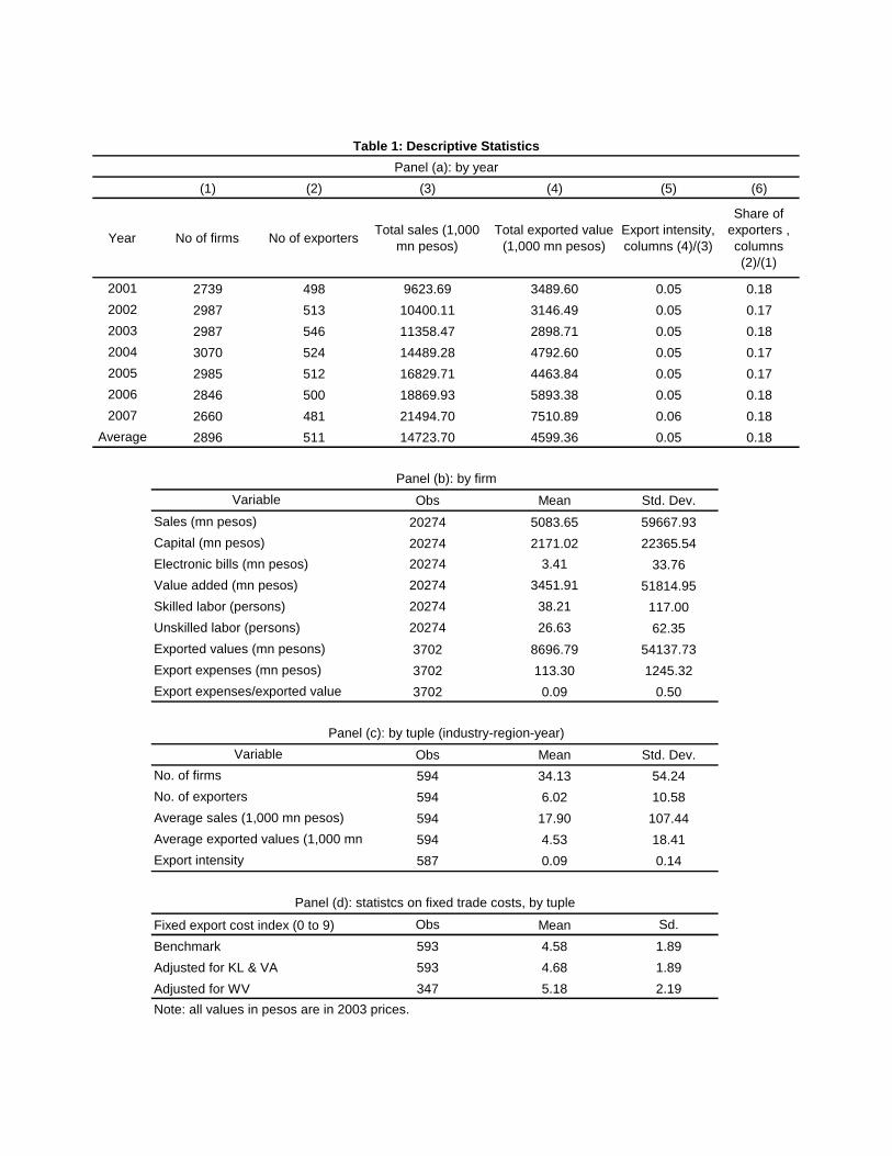
********* Table 1 about here *********
Panel (a) of Table 1 reports annual statistics.16 Our data cover 2,896 firms in an average year,18% of which are exporters. Sales and exported values rise over the seven years. Switching between
14g > 2 is assumed to ensure a finite variance of A; see, e.g., Helpman, Melitz, and Yeaple (2004) for similar use.15Earlier versions of this dataset have been used by Levinsohn (1999), Pavcnik (2002), and Lopez (2008), among
others.16We drop multinational subsidiaries and licensees in regressions, since their export behaviors are heavily influenced
by their overseas parent firms. The included industries (ISIC-Rev.3 codes) are 17, 18, 19, 20, 21, 22, 24, 25, 26, 27,28, 29, 30, 31, 32, 33, 34, 35, 36.
7
exporters and nonexporters is rare and happen nearly only to frequent switchers.17 Panel (b) reportsfirm-level statistics. The variable export expenses contains all relevant expenses (including tariffpayments) that firms incur in the exporting process. On average, export expenses are equal toapproximately 9% of exported values of an average exporter. We will revisit export expenses inthe next section. Panel (c) of Table 1 reports statistics at the industry-region-year (tuple) level, atwhich our fixed export costs are constructed.
There are three groups of control variables used in this study. (1) Firm-level control variables,including capital/labor ratio (KL) and value added ratio (VA),18 are computed using variablesreported by the ENIA. (2) Regional and industrial characteristics are obtained from the EstadísticasVitales and Carabineros.19 (3) The productivity measure, total factor productivity or TFP inlogarithm, is estimated using the Ackerberg-Caves-Frazer (2006) method, which builds on theOlley-Pakes (1996) and Levinsohn-Petrin (2003) methods.20 The TFP has been standardized usingindustry-year mean and standard deviation: TFP ST AN
jt = [TFPji − µ(TFP )it]/σ(TFP )it. Thestandardization is to ensure the comparability of TFP across industries. In the rest of the paper,the standardized TFP is used unless noted otherwise.
3.2 Measurement of fixed trade costs
In this section, we construct indices that measure the fixed export costs associated with eachindustry-region-year (irt) tuple. The construction of the index consists of two steps. The firststep is to regress exporters’ export expenses on their export volumes and extract the fixed effectsassociated with each industry, each region, and each year. Exporters in the ENIA report expensesresulting from exporting activities for each year, denoted by ExportExpensesjt, with j as the firmidentifier. This variable is a remarkable feature of the ENIA data, considering that export costs arerarely reported in firm-level datasets available to empirical economists. Meanwhile, this variable isnot readily usable because it includes all the costs incurred by exporting, without distinguishingfixed from variable costs.
Export expenses have a fixed component and nonfixed components that include tariff andnontariff payments. Tariff rate and export volume are denoted by τ ≥ 0 and V > 1, respectively.To distinguish fixed export costs from nontariff ones, we specify a regression of ln ExportExpenses
reported by exporters:21
17See Appendix A1. The frequent switchers are likely subcontracting manufacturers.18Value-added ratio is defined as value added divided by total sales.19Publicly available at http://www.ine.cl/canales/chile_estadistico/.20TFP using methods along this line are widely used in the trade literature. See, e.g., Amiti and Konings (2007),
Goldberg, Khandelwal, Pavcnik, and Topalova (2010), Greenaway, Guariglia and Kneller (2007), Javorcik (2004),Javorcik and Spatareanu (2008, 2011), Kasahara and Rodrigue (2008), Park, Yang, Shi, and Jiang (2010), andTopalova and Khandelwal (2011). In particular, for the use of the Ackerberg-Caves-Frazer method, see Arnold,Javorcik, Lipscomb and Mattoo (2008), Javorcik and Li (2008), and Petrin and Sivadasan (2011).
21The foundation for regression (8) is as follows. Export expenses is equal to
ExportExpenses = ef+ζ1 ln V +ζ2 ln(1+τV ).
This exponential form with linearly added covariates follows the literature, see e.g., Anderson and van Wincoop
8
ln ExportExpensesjt = δi + δr + δt + ζ1 ln(1 + Vjt) + ζ2 ln(1 + τitVjt) (8)
+(ζ3i + ζ3r + ζ3t) ln(1 + Vjt) + ζ4FirstT ime + ϵjt,
where i, r, and t are industry, region, and year identifiers, respectively. {δi, δr, δt} are the fixedeffects specific to industry i, region r, and year t, respectively. To isolate them from the industry-,region-, or year-specific factors that affect export expenses through export volume, we control forfixed effects in the coefficient of ln Vjt by including ζ3i, ζ3r, and ζ3t. τit is at the industry-yearlevel, proxied by weighted tariff-equivalent trade barrier for Chile’s five largest trade partners (seeAppendix A2 for details). First-time exporters, which are small in number, may pay different exportexpenses and thus we also include a first-time exporter dummy variable FirstT ime.22 Figure 4 isthe histogram of residuals derived from regression (8), a distribution that appears similar to thenormal distribution.
********* Figure 4 about here *********
The unit of export volume is ambiguous both here and in the literature. Export volume in theliterature normally refers to exported value, following which regression (8) is specified. Nevertheless,the export volume more relevant to export expenses could be in terms of quantity or weight, andwe keep an agnostic view toward which is the “true” export volume, and pragmatically developtwo alternative specifications as robustness checks. The first alternative is to add the capital-laborratio KL and the value-added ratio V A of firms into regression (8). If the “true” export volumeis in terms of quantity, these two ratios help to control for the price variation in ln(1 + Vjt).23
The second alternative is to add the weight/value ratio, denoted by (WV )it for industry i and year
t, into regression (8). If the “true” export volume is in terms of weight, these two ratios help tocontrol for the weight/value ratio variation in ln(1+Vjt).24 We extract the value/weight ratio of USimports from Chile via ocean shipments, reported in Hummels (2007) to proxy for (W
V )it. Hummels’(2007) data do not cover the years 2005-2007 such that we have more missing values when thisspecification is used. Notably, due to this ambiguity, we refrain from giving specific meaning (e.g.,variable export costs and transport costs) to the the coefficients of ln Vjt in regression (8).
(2004)’s review article (p.710), Anderson and Yotov (2010) and Limão and Venables (2001). It becomes, in log terms,
ln ExportExpenses = f + ζ1 ln V + ζ2 ln(1 + τV ).
The regression is run on exporters, i.e., V >0. Notice that the unit of V is 1,000 pesos, such that ln(V + 1) can stillbe negative. Thus, in regression (8), we use ln(V + 1) instead of ln V .
22Their small number (see Appdendix 1 for details), as well as the fact that the majority of them are frequentswitchers, keeps us from estimating a sunk cost parameter that varies by tuple.
23In this case, let qjt be the export volume of firm j in year t. Suppose ln(1 + Vjt) = ln(pjtqjt) = ln pjt + ln qjt,where pjt and ln qjt are the price and quantity of firm j’s output in year t. Assume pjt = p(KLjt, V Ajt), thencontrolling for KL and VA holds ln pjt constant.
24In this case, Wjt is the export volume. Let Vjt be the positive export volume. Suppose ln Wjt = ln[( WV
)it×(Vjt)] =ln( W
V)it + ln Vjt; then ln Vjt = ln Wjt − ln( W
V)it follows.
9
Regression (8) indicates that given zero volume, exporters still pay the export expenses δi +δr + δt, which are fixed but unsunk export costs. In other words, δi + δr + δt are the counterfactualfixed export costs that nonexporters would necessarily pay if they had exported. In the secondstep, we match each tuple (irt) to an fixed export cost value δirt = δi + δr + δt and transform itinto an index that ranges between 0 and 9:
firt = δirt − minirt{δirt}maxirt{δirt} − minirt{δirt}
× 9. (9)
In the following analysis, a firm, regardless of its export status, can be linked to its tuple’s firt. Sincethree different specifications are used to estimate {δi, δr, δt}, there are three indices constructed,labeled as benchmark, KL and VA adjusted, and WV adjusted, respectively. Their distributions aredisplayed in Figure 5. The benchmark and KL & VA adjusted indices show close similarity withnormal distribution, while the VW adjusted index shows a larger fraction of large values.25
********* Figure 5 about here *********
We depict in Figure 6, as a preliminary reality check, the 25th and 75th percentiles of fixedexport costs by industry, region and year, respectively. In panel (a), fixed export costs are shown tobe high in the industries that manufacture products of wood, transportation equipments, machineryand basic metals, because firms in these industries usually need facilities that can ship sizable cargos;in contrast, the manufacturing of communication and office equipments as well as furniture, shownwith low fixed export costs, can be transported using ordinary facilities. Panel (b) of Figure 6demonstrates a large dispersion of fixed trade costs among 13 administrative regions of Chile.26
Panel (c) indicates that fixed export costs were trending down between 2001 and 2007, whichwas likely due to nationwide improvements in trade-related infrastructure;27 the downturn in fixedexport costs was particularly significant in the year 2003, when Chile’s recession hit its bottom.
********* Figure 6 about here *********
Notably, firt is constructed using three single fixed effects {δi, δr, δt} rather than tuple fixedeffects δirt or duple fixed effects {δir, δrt, δit}. The reasons are twofold. First, tuple and duple assets of firms have too few observations. A median tuple has only two exporters, while median duplesir, rt, and it have 10, 11, and 26 exporters, respectively. Considering the total number of exporters3,702, duple and tuple fixed effects are far fewer than enough to identify informative parameterson fixed export costs. The second reason is the tuple and duple peculiarities that may bias theestimation. Take the tuple fixed effects for example. A region r′ may in year t′ have industrialpolicies favorable to industry i′, which affects the fixed effect of the tuple i′r′t′, as well as export
25This irregularity is not very surprising given that the WV adjusted index covers only four out of seven years.26Chile was divided into 13 administrative regions in 1974. This division was revised in 2007. To maintain
consistency throughout the sample, we use the 1974 division.27For example, between 1993 and 2006, Chile invested $5.9 billion in transport infrastructure and built 2,505
kilometers of roads. See OECD (2009a, p.70) for details.
10

decisions in the tuple; consequently, it would be difficult to tease out the the policy-driven fixedcost reduction and policy-driven export increase. The same argument applies to other peculiarities,such as shocks to weather, local labor and shipment-service markets.
3.3 Checks on the fixed export cost indices
Before using the fixed export cost indices estimated above in empirical analysis, we check (1)whether they are based on a reasonable functional form, (2) their relationship with firm-levelidiosyncrastic export expenses, and (3) the source of their variation. In fact, several more checkson these indices are undertaken, though they are more relevant to the testing of the three hypothesesand thus placed in Section 4.
The first check is concerned about the linear functional form of regression (8). Regression(8) is based on the assumption that export expenses have two components, fixed and variable. Thefirst check asks what if the construction of fixed export cost index does not account for exportvolume. We hypothesize that the resulting fixed export cost index will then be correlated withexport volume; in other words, the fixed export cost index will be non-fixed. We test this byrunning regression (8) without the export volume term ln V , then use its estimates to constructan experimental fixed export cost index, and lastly regress this index on tuple-level average exportvolume. This experimental index, as shown in column (1) of Table 2, rises with export volume. Incontrast, the three indices constructed earlier are shown in columns (2)-(4) to have no correlationwith export volume.
********* Table 2 about here *********
The second check is to determine how much the three indices are influenced by idiosyncraticexport expenses paid by firms. The contents of these expenses, as the term idiosyncrasy suggests,are unclear; they possibly include costs that firms incur to break into certain foreign markets,bribes paid to some foreign customs officials, product samples given to foreign clients and othercosts resulting from marketing and sales.28 A skeptic may wonder whether such idiosyncrasies arepicked up by the three indices. Assuming time-invariant idiosyncratic export expenses of firms, wedevelop a check that can detect the correlation between idiosyncratic export expenses paid by firmsand the three indices. We first estimate firm fixed effects in export expenses,29 then average themat the industry-region duple level, and lastly examine their correlation with the indices that are
28Export expenses paid in foreign markets, if firm-specific, are not absorbed into {δi, δr, δt}. Take δi of industryi for example. It does not capture the entry costs paid by some exporters of industry i in a given foreign market,unless all exporters of industry i serve that foreign market (if all firms in industry i do serve that foreign market,the entry cost for that market is in effect a local cost because serving that market is a common practice in industryi and therefore should arguably be included in δi). The same reasoning holds for δr and δt.
29Specifically, we estimate
ln ExportExpensesjt = δj + ζ1 ln Vjt + ζ2 ln(1 + τitVjt) + ζ3F irstT ime + ϵjt,
where over tildes distinguish the coefficients from those in regression (8); next, we extract the estimates {δj}j andscale them between 0 and 9.
11

likewise averaged: fir· = 1T
∑Tt=1 firt. A positive correlation between the two would indicate that
the indices are driven by local firms’ idiosyncratic expenses.
********* Table 3 about here *********
Table 3 reports the correlation between the averaged indices and averaged firm-year fixed effects.Positive correlation is not detected between the two variables, either with or without controllingfor averaged capital-labor ratio and value-added ratio of firms. Notably, higher indices are positiveassociated with capital-labor ratio, possibly because selling capital intensive products, opposite ofChile’s comparative advantage, is relatively incompatible with local infrastructure (e.g., transportfacilities). The correlation between trade and infrastructure has been documented in the litera-ture.30 We now further look into this as the third check, a reality check that pinpoints (1) whatfactors can explain the variation in the fixed export cost indices and (2) whether the indices areconsistent with findings from external data sources.
Specifically, we link the three indices to the World Bank Enterprise Surveys (WBES). TheWBES evaluates business environments in nearly all developing countries by tracking a representa-tive sample of local firms. The WBES undertook surveys in Chile in 2006 and 2010. We choose the2006 survey because it overlaps with our ENIA sample period. Next, we average the firm responsesto the industry-region level that can be matched to the indices {firt}t=2006. Here, we use only thebenchmark and KL & VA adjusted indices, because the WV adjusted index does not cover the year2006. For either of the two indices, we regress it on the responses to each relevant survey question.The questions are listed in the first column of Table 4, and the coefficients are summarized in therest of the columns.
Notably, some of the questions seem to be about regional characteristics, but the perceivedfacts and thus the responses can vary across industries; the same hold for questions that give theimpression of industrial characteristics. Therefore, we run each regression with three specifications:with no fixed effects, with region fixed effects, and with industry fixed effects.
********* Table 4 about here *********
The results are reported in Table 4. Fixed export costs are found to higher where there arefrequent power outages, fewer competitors, more informal-sector competitors, more licensing andpermits requirements as well as customs and regulations. The coefficients are self-explanatory,though we would like to make three observations. First, not all respects of business environmentare significantly under every specification, because the WBES business environment indicators donot necessarily vary along both industry and region dimensions. For example, frequent poweroutage as an important indicator of weak infrastructure affects all industries and regions, suchthat it is significantly associated with fixed export costs under all three specifications; in constrast,
30See, e.g., Bougheas, Demetriades, and Morgenroth (1999), Blonigen and Wilson (2008), Clark, Dollar, and Micco(2004), Donaldson (2010), Limão and Venables (2001), and Wilson, Mann, Otsuki (2003).
12

business licensing and permits is related to nationwide regulations, the variation of which is mainlyacross industries, loses significance when industry fixed effects are included.
Second, fixed export costs are correlated with a mix of business environment indicators, includ-ing but not limited to infrastructure. As Table 4 illustrates, institutions, regulations, and marketstructure also matter; thence, high fixed export costs should not be equated to weak infrastruc-ture.31 In fact, fixed export costs are shown to be higher in regions where transportation is lessviewed as the most severe obstacle, possibly because regions with high fixed export costs have moresevere obstacles, such as rampant competition from the informal sector. Third, fixed export costsare high where there are fewer competitors [in the formal sector], but more competitors in the infor-mal sector. We speculate that competitors in the formal sectors may share some fixed export costs,because for example the construction of transport facilities can be economized by a large numberof users. This is not the case of competitors in the informal sector, who may take advantage ofthe positive externality spilled over by formal-sector firms; this said, rampant competition from theinformal sector may actually raise local fixed export costs.
4 Empirical Evidence
This section tests Hypotheses I to III. Hypothesis I is the focus. We start with a reduced-formregression and next examine four issues that may disturb the reduced-form identification. Theexamination results corroborate the reliability of the specification, which is then applied to the testof Hypothesis II. Last, we test Hypothesis III, a direct implication of Hypothesis I that helps tounderstand the role of fixed export costs in aggregated trade data.
4.1 Hypothesis I
Equation (5) in the theoretical model can be transformed into a binary dependent variable regres-sion32
Pr(Xjt = 1) = Ψ[βf firt + βT F P TFPjt + λ′Zfirt + ujt], (10)
where as before j, i, r, t are identifiers for firms, industries, regions, and years, respectively, andZfirt is a vector of control variables and fixed effects along various dimensions. Hypothesis I claimsβf < 0 and βT F P > 0.
********* Table 5 about here *********31The quality of infrastructure is not a good indicator of fixed export costs also because it affects both fixed and
variable export costs. Put more generally, export costs can be categorized into four types that are mutually exclusiveof each other: (i) fixed export costs driven by infrastructure, (ii) variable export costs driven by infrastructure, (iii)fixed export costs not driven by infrastructure, and (iv) variable export costs not driven by infrastructure. Measuresof trade-related infrastructure pinpoint types (i) and (ii), while our fixed export cost measure captures types (i) and(iii). Our index construction deliberately expunges variations in export expenses driven by variable export costs, andthus pin down variations in infrastructure and institutions that impact fixed export costs.
32The steps in footnote 12 are reproduced here. Pr[X = 1] = Pr[π ≥ u] = Ψ[π]. When π ≥ 1, Ψ[π] follows astandard normal distribution Φ(π); when π < 1, Ψ[π] = 0, a case that also coincides with Φ(π), with the 1 absorbedby the constant term of the probit model.
13
Table 5 reports the results. Columns (1) does not include control variables. Based on column(1), columns (2) controls for firm-level capital-labor ratio KL and value-added ratio VA. Column(3) further includes (i) tariff rates (industry-year level) to control for the impacts of global tradeliberalization, and (ii) crime rates and infant death rates to control for regional infrastructure. Wehave also included in all three columns industry and year fixed effects to control for Chile’s industrialcomparative advantage and possible macroeconomic shocks.33 Hypothesis I receives supports fromall the three columns. We further experiment with the fixed export cost index lagged by one year,as well as indices adjusted for KL & VA and VW; they lead to very similar results in columns(4)-(6).
In Table 5, the regression using each index is run with and without control variables, a tech-nically simple exercise that involves a complex tradeoff. In columns (1)–(2), we do not control forinfrastructure because it affects fixed export costs as shown earlier and therefore tends to shrinkthe the magnitude of βf . Later, in columns (3)–(6), we include them because they may also affectexport decision through variable export costs. This said, whether to include them is a little dilem-matic. Fortunately, the coefficients hardly change across columns (1)–(3). We will later revisit theconfounding effect of variable export costs. As discussed earlier, the fixed export cost indices reflectthe recurring fixed export costs that exporters have to pay per period. Paying them is necessarybut perhaps insufficient for a nonexporter to start exporting. Assumptions have to be made onhow sunk costs spread over a firm’s export-activity cycles, on which structural estimation may haveadvantages. This will be an interesting avenue for future research.
********* Table 6 about here *********
Table 6 presents the marginal effects of fixed export costs on export decisions based on thecoefficients estimated in columns (3), (5), and (6) of Table 5, where the βf ’s are conservative inmagnitude as discussed above. Take column (3) for example. Moving from the 25th percentile tothe 75th percentile, fixed export costs rise by 49.7 percent (1.590/3.198), and the export propensityof firms decreases by two percentage points, equivalent to a 12 percent change (0.02/0.17). Whenthe KL and VA adjusted index used, the two magnitudes are respectively 46.7 percent and 12percent. When the WV adjustment applied, 41.6 percent and 6 percent, though the magnitude ofthe WV-adjusted fixed export costs is less accurate as discussed early. Evidently, other factors heldconstant, fixed export costs lead to a nontrivial change in export propensity.
Reverting to regression (10), we next examine four identification issues to which the regressionmight be exposed. It is helpful at this point to clarify the meaning of identification in this context.Identification, usually alluding to causality in the literature, here refers to whether the correlationcaptured by the βf in regression (10) is indeed between export propensity and fixed export costs.We do not argue for a causal effect of fixed export costs because tuple-level fixed export costs areclearly not randomized. Therefore, we do not consider endogenous locational choices made by firmsor the efforts made by exporters to reduce local fixed export costs as identification concerns in this
33Region fixed effects are not used because regional control variables used here vary little over time.
14
study. Put differently, the fact that exporters choose places with low fixed export costs to reside ormake efforts to lower local fixed export costs has already indicated the association between fixedexport costs and export decisions. The identification issues that we address below are, specifically,whether the estimated correlation between export propensity and fixed export costs is driven byour sample (issue 1), index construction (issue 2), regression techniques (issue 3), or confoundingeffects of variable export costs (issue 4).
1. By industry study We first check whether the findings from Table 5 hold for individ-ual industries, as an alternative approach to using standardized TFP. In general, there are twoapproaches to address the incomparability of TFP across industries. One is to standardize theTFP of each industry using its mean and standard deviation as done above. By doing so, TFP istransformed to be comparable across industries,34 because the standardized TFP of a firm is aboutits standing relative to its peers within the industry. For example, a firm that is one standarddeviation more productive than the industry mean is equally recognized regardless of its industry,and the differences in industry means have been accounted by the industry fixed effects. The meritof this approach is the usage of the full sample.
********* Table 7 about here *********
The alternative approach is to run regressions using individual industries. This approach doesnot transform data but substantially reduces sample size. In table 7, we run regression (10) forfour largest industries, which in total account for 35% of the total sample size. These individualindustries lead to similar findings. The industry “publishing, printing and reproduction of recordedmedia” is associated with the largest βf in magnitude. The printing industry, compared to otherthree, relies more heavily on design, reputation, and communication, which possibly explain whyits export propensity is more sensitive to fixed export costs.
2. Applying estimated fixed export costs to nonexporters The fixed export cost indicesfor nonexporters are compiled using those of exporters. One may worry that exporters are more (orless) efficient than nonexporters in managing costs, such that fixed export costs paid by exporters donot represent the fixed export costs that non-exporters would pay if they had exported. To addressthis, we conduct an experiment that assumes that fixed export costs perfectly discriminate amongfirms based on their characteristics: productivity, employment, total sales, and total value added.Specifically, the first step is to use the sample of exporters to estimate a correlation between theindices and a standardized firm characteristic yjt: firt = ωyjt(Xjt = 1)+ εirt, and the second step isto average εirt, the residuals obtained from the first step to generate a new tuple-level index. If firt
is just the fixed export costs of local high-performing firms, the results from using firt in Table 5will not hold when firt is used instead. The new results are reported in Table 8, in which each paneluses a different fixed export cost index and each column uses a different firm characteristic. The
34We looked into the distribution of TFP both prior to and after standardization and did not find systematicaldifference. Details are available upon request.
15

coefficients are close to those in Table 5, in both magnitude and significance levels. Notably, thedrawbacks of using firt are its hypothetical nature and the difficulty in interpreting the magnitudeof firt’s coefficient in the regression; therefore, firt serves only in this robustness check.
********* Table 8 about here *********
3. Fixed export costs of high-productivity nonexporters The Probit model, such asregression (10), treats exporters and nonexporters as export decisions, about which one may feelconcerned because the difference in fixed export costs between exporters and nonexporters do notnecessarily link to the relevance of fixed export costs to export decisions. We next adopt a secondempirical approach that focuses on high-productivity nonexporters. The theory underpinning thisapproach has been discussed in Section 2 as an alternative version of Hypothesis I. In essence, thisapproach asks whether high-productivity nonexporters face high fixed export costs.
We examine the productivity distribution of exporters for a criterion for “high productivity.”Recall that a firm has a high export propensity if it has either a high productivity or a low fixedexport cost; in other words, exporters may not have high productivity though exporters are onaverage more productive than nonexporters. As a compromise, we choose the productivity of the75th percentile exporter in a given industry as the criterion for “high productivity;” in other words,a nonexporter is defined as a high-productivity one if it is no less productive than the 75% percentileproductivity of exporters in its industry.
With the high-productivity nonexporters pinpointed, we compare their fixed export costs withthose of exporters. The preliminary results have been reported in Figure 1 as discussed in the intro-duction. Figure 1 shows the productivity distribution of exporters and nonexporters, respectively,in two industries with the largest number of observations (“fabricated metal products” and “woodand cork”).35 It conveys two messages. First, there exist in both industries high-productivity non-exporters, which are more productive than the 75th percentile exporters. Second, according to thet-statistics, high-productivity exporters face higher fixed export costs than the exporters that areless productive than them.
********* Table 9 about here *********
Now we undertake a more detailed look at the comparison of fixed export costs between high-productivity nonexporters and exporters. We divide exporters into ten productivity deciles; anexporter is more productive if it is in a higher decile. Table 9 examines the industry “fabricatedmetal products.” We compare the fixed export costs of high-productivity exporters with those ofall exporters (column (1)), those in deciles 1-4 (column (2)), those in deciles 5-8 (column (3)),those in decile 9-10 (column (4)), and those in decile 10 (column (5)). Clearly, high-productivitynonexporters face higher fixed export costs than all exporters except those in deciles 9 and 10. Thesame finding is reached when adjusted fixed export cost indices are used. Table 10 examines the
35Since only one industry is examined, the TFP is not standardized.
16

industry “wood and cork,” which shows still stronger results: high-productivity nonexporters facehigher export fixed costs than nearly all exporters (two exceptions in panel (c)).
********* Table 10 about here *********
4. Fixed export costs vs. variable export costs The fourth identification issue is whetherβf in regression (10) is contaminated by the negative effect of variable export costs on Pr(Xjt = 1).Conceivably, fixed export costs are higher where variable export costs are high, which is the reasonwhy we control for infrastructure quality in regression (10). To further address this, we examinethe correlation between fixed export costs and firm-level export volume using the regression
ln(Vjt + 1) = κf firt(j) + κT F P TFPjt + ξ′Zjirt + ηjt, (11)
where Vjt ≥ 0 is the export volume of firm j in year t, and other notations are the same as inregression (10). If fixed trade costs capture the effect of variable export costs, we would see anegative and significant κf ; namely, a negative association between firm-level export volume andfixed export costs.
********* Table 11 about here *********
A noteworthy issue on the estimation of regression (11) is its truncated dependent variable: exportvolume is truncated at zero and this causes inconsistent estimates of all parameters. Thence, wejointly estimate regression (11) with regression (10) using a Type II Tobit model, which assumesthat, conditional on (f , TFP , Z), (u, η)′ follows distribution N((0, 0)′, Σ), where
Σ ≡(
σ2N ρσN
ρσN σ2N
).
This joint model integrates the estimation of two export behaviors: (i) whether to export and (ii) ifto export, how much is the volume. (i) and (ii) correspond to regressions (10) and (11), respectively.The results are reported in Table 11.36 As in Table 5, we have experimented with all three indices.βf and βT F P are both significant and respectively negative and positive, just as in Table 5, attestingagain to the effects of fixed exports costs and TFP on export propensity. In contrast, in the export-volume regression, κf , the coefficient of fixed export costs, is not significantly different from zero,while κT F P > 0 is significant, being consistent with the theoretical result that fixed export costsdo not affect export volume.37 Thus, our fixed export cost measure is unlikely to have capturedthe negative effect of variable export costs on export decisions.
36It is difficult to find convincing tuple-level instruments that affect export decisions but not export volumes.Therefore, we use nonlinearity to identify the effect of selection. See Cameron and Trivedi (2009, p.543) for adiscussion on this.
37ρ is positive and significant, indicating that regression (11) is not independent from regression (10) and thussample selection needs to be corrected.
17
4.2 Hypotheses II and III
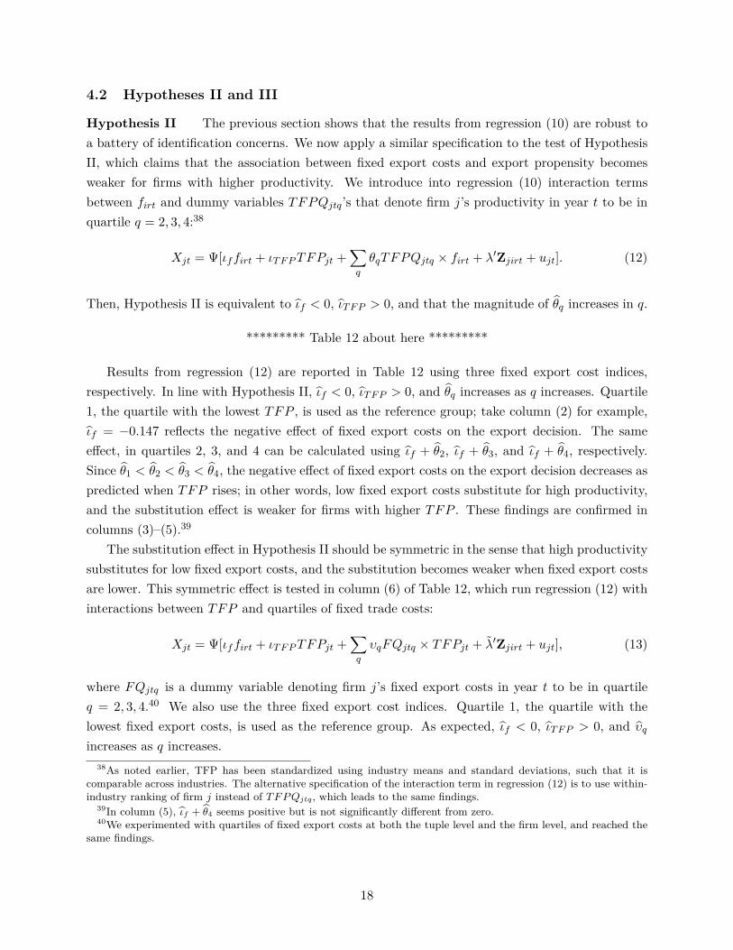
Hypothesis II The previous section shows that the results from regression (10) are robust toa battery of identification concerns. We now apply a similar specification to the test of HypothesisII, which claims that the association between fixed export costs and export propensity becomesweaker for firms with higher productivity. We introduce into regression (10) interaction termsbetween firt and dummy variables TFPQjtq’s that denote firm j’s productivity in year t to be inquartile q = 2, 3, 4:38
Xjt = Ψ[ιf firt + ιT F P TFPjt +∑
q
θqTFPQjtq × firt + λ′Zjirt + ujt]. (12)
Then, Hypothesis II is equivalent to ιf < 0, ιT F P > 0, and that the magnitude of θq increases in q.
********* Table 12 about here *********
Results from regression (12) are reported in Table 12 using three fixed export cost indices,respectively. In line with Hypothesis II, ιf < 0, ιT F P > 0, and θq increases as q increases. Quartile1, the quartile with the lowest TFP , is used as the reference group; take column (2) for example,ιf = −0.147 reflects the negative effect of fixed export costs on the export decision. The sameeffect, in quartiles 2, 3, and 4 can be calculated using ιf + θ2, ιf + θ3, and ιf + θ4, respectively.Since θ1 < θ2 < θ3 < θ4, the negative effect of fixed export costs on the export decision decreases aspredicted when TFP rises; in other words, low fixed export costs substitute for high productivity,and the substitution effect is weaker for firms with higher TFP . These findings are confirmed incolumns (3)–(5).39
The substitution effect in Hypothesis II should be symmetric in the sense that high productivitysubstitutes for low fixed export costs, and the substitution becomes weaker when fixed export costsare lower. This symmetric effect is tested in column (6) of Table 12, which run regression (12) withinteractions between TFP and quartiles of fixed trade costs:
Xjt = Ψ[ιf firt + ιT F P TFPjt +∑
q
υqFQjtq × TFPjt + λ′Zjirt + ujt], (13)
where FQjtq is a dummy variable denoting firm j’s fixed export costs in year t to be in quartileq = 2, 3, 4.40 We also use the three fixed export cost indices. Quartile 1, the quartile with thelowest fixed export costs, is used as the reference group. As expected, ιf < 0, ιT F P > 0, and υq
increases as q increases.38As noted earlier, TFP has been standardized using industry means and standard deviations, such that it is
comparable across industries. The alternative specification of the interaction term in regression (12) is to use within-industry ranking of firm j instead of T F P Qjtq, which leads to the same findings.
39In column (5), ιf + θ4 seems positive but is not significantly different from zero.40We experimented with quartiles of fixed export costs at both the tuple level and the firm level, and reached the
same findings.
18
One may worry about the practice of dividing firms by their firt and TFPjt quartiles, becausefirt is not a firm-level variable and the comparability of TFP across industries relies on standard-ization. In column (7), we interact firt directly with TFPjt . In column (8), we replace TFPjt
using the productivity percentile of a firm within its industry-year; that is, the most (least) pro-ductive firm in an industry-year will be at the 100th (0th) percentile. The interaction terms inboth columns are negative, in line with Hypothesis II. We also use the residual-based fixed exportcost indices to examine the interaction, which lead to the same findings (reported in Table A3).
The relationship between Table 12 and Tables 9–10 deserves elaboration. The findings fromTables 10–11 will be still stronger if the findings from Table 13 are taken into account. As shownabove, high-productivity firms respond to fixed export costs less than low-productivity firms whenmaking export decisions. However, high-productivity nonexporters are evidently still blocked fromexporting by fixed export costs. This is because the total effect rather than the marginal effect offixed export costs matters for export decisions, and lends further support to the negative effect offixed export costs on export decisions.
Hypothesis III Hypothesis III claims that exporters export a larger volume if either (i) fixedexport costs are higher or (ii) dispersion of productivity is larger. Intuitively, with fixed exportcosts held constant, a larger dispersion of productivity leads to more firms that are “beyond thethreshold;” given the dispersion constant, higher fixed export cost raises the threshold. Below wesubmit this hypothesis to empirical testing. Fixed export costs of tuples have been estimated, andwe now compile the coefficient of variation (CV), i.e., the standard deviation to the mean, of TFPfor each tuple.41 The dependent variable is the logarithm of total exports divided by number ofexporters at the tuple level. Since it is an average, we weight the regression using the inversednumber of exporters at the tuple level.
********* Table 13 about here *********
The results are reported in Table 13. Column (1) includes the CV of productivity but not thefixed export cost index. Tuples with a larger dispersion of productivity are shown to have averageexporters that export larger volumes. On the contrary, columns (2) includes the benchmark fixedexport cost index but not the CV of productivity; clearly, higher fixed export costs are associatedwith a larger average export volume. Column (3) includes both of the two variables and the findingsfrom columns (1)–(2) remain, while their magnitudes both shrink slightly. We repeat columns (2)–(3) using the adjusted fixed export cost indices in columns (4)–(7) and reach the same results. Thecoefficients of control variables are consistent with expectation. Notably, crime rate has a slightlypositive correlation with average export volume, possibly because organized crimes usually clusteraround port areas where fixed export costs happen to be low.
The linkage between Table 13 and Table 11 is noteworthy. Higher fixed export costs affect exportvolume of average exporters by selecting firms with higher productivity to be exporters, but this
41Since CV is an industry-specific measure, it is constructed using non-standardized TFP.
19

mechanism does not affect firm-level export volume conditional on productivity. As theoreticallyillustrated in Section 2, f , once paid, does not affect export behavior any more; this has beenempirically shown in Table 11, where productivity is controlled for. If productivity is not controlledfor, the selection effect in Table 13 should present itself in regressions of firm-level export volume.We undertake this experiment and report the results in Table A4, where exporters in tuples withhigher fixed export costs are shown to export larger volumes when productivity is not controlledfor.
5 Conclusions
Firm-level export decisions essentially depend on two cost parameters: average variable costs ofproduction (i.e., productivity) and the fixed costs of selling products abroad (i.e., fixed export costs).This paper closes a gap of the literature by empirically showing that both of them are associatedwith export decisions of firms. There are high-productivity nonexporters and low productivityexporters, the former of which face higher fixed export costs than the latter. The two parametersalso interact with each other at the margin: the effect of lowering fixed export costs on exportpropensity is weaker for a firm with higher productivity. Also, the average export volume ofexporters is larger where the dispersion of productivity is larger and the fixed export costs arehigher. We also document that fixed export costs vary with a list of factors including but not limitedto infrastructure quality, and fixed export costs are negatively associated with export propensitybut not with export volume. These findings indicate fixed export costs to be an independentparameter that affects export performance.
There are both theoretical and empirical avenues for future research. On the theoretical side,it would be interesting to examine how productivity and fixed export costs are jointly determinedat the firm level. This paper has shown that exporters, if located where fixed export costs are low,do not need high productivity to reach foreign markets. To date, the determinants of productivityand fixed export costs remain poorly understood, and this paper provides a new perspective.On the empirical side, our fixed export cost measures can be used to determine the efficiency ofbusiness environment improvements. This paper suggests that encouraging exports and promotingproductivity growth can be two very different goals. To encourage exports, it may suffice to reducelocal fixed export costs, while promoting productivity growth may involve more structural reforms.
References
[1] Ackerberg, Daniel A.; Caves, Kevin and Frazer, Garth. 2006. “Structural Identificationof Production Functions.” Working paper.
[2] Amiti, Mary and Konings, Jozef. 2007. “Trade Liberalization, Intermediate Inputs,and Productivity: Evidence from Indonesia.” American Economic Review 97(5): 1611-1638.
20

[3] Anderson, James E. and van Wincoop, Eric. 2003. “Gravity with Gravitas: A Solutionto the Border Puzzle.” American Economic Review 93(1): 170-192.
[4] Anderson, James E. and van Wincoop, Eric. 2004. “Trade Costs.” Journal of EconomicLiterature 42(3): 691-751.
[5] Arkolakis, Costas. 2010. “Market Penetration Costs and the New Consumers Marginin International Trade.” Journal of Political Economy 118(6): 1151-11.
[6] Arnold, Jens Matthias; Javorcik, Beata; Lipscomb, Molly and Mattoo, Aaditya. 2008.“Services Reform and Manufacturing Performance: Evidence from India.”
[7] Bernard, Andrew B. & Bradford Jensen, J., 1999. “Exceptional exporter performance:cause, effect, or both?” Journal of International Economics 47(1): 1-25.
[8] Bernard, Andrew B. and Jensen, J. Bradford. 2004. “Why Some Firms Export.” Reviewof Economics and Statistics 86(2): 561-569.
[9] Bernard, Andrew B.; Eaton, Jonathan; Jensen, J. Bradford and Kortum, Samuel.2003. “Plants and Productivity in International Trade.” American Economic Review93(4): 1268-1290.
[10] Bernard, Andrew B.; Jensen, Bradford J. and Schott, Peter K. 2006. “Trade costs,firms and productivity.” Journal of Monetary Economics 53(5): 917-937.
[11] Blonigen, Bruce A. and Wilson, Wesley W. 2008. “Port Efficiency and Trade Flows.”Review of International Economics 16(1): 21-36.
[12] Bougheas, Spiros; Demetriades, Panicos O. and Morgenroth, Edgar L. W. 1999. “In-frastructure, transport costs and trade.” Journal of International Economics 47(1):169-189.
[13] Cameron, A. Colin and Trivedi, Pravin K. 2005. Microeconometrics: Methods andApplications. Cambridge University Press, New York.
[14] Chaney, Thomas. 2008. “Distorted Gravity: The Intensive and Extensive Margins ofInternational Trade.” American Economic Review 98(4): 1707-21.
[15] Clark, Ximena; Dollar, David and Micco, Alejandro. 2004. “Port efficiency, maritimetransport costs, and bilateral trade.” Journal of Development Economics 75(2): 417-450.
[16] Das, Sanghamitra; Roberts, Mark J. and Tybout, James R. 2007. “Market EntryCosts, Producer Heterogeneity, and Export Dynamics.” Econometrica 75(3): 837-873.
[17] De Loecker, Jan. 2007. “Do exports generate higher productivity? Evidence fromSlovenia.” Journal of International Economics 73(1): 69-98.
21

[18] Donaldson, Dave. 2010. “Railroads of the Raj: Estimating the Impact of Transporta-tion Infrastructure.” Working paper.
[19] Eaton, Jonathan; Kortum, Samuel and Francis Kramarz. 2011. “An Anatomy of In-ternational Trade: Evidence From French Firms.” Econometrica 79(5): 1453-1498.
[20] Goldberg, Pinelopi K.; Khandelwal, Amit K; Pavcnik, Nina and Topalova, Petia. 2010.“Multiproduct Firms and Product Turnover in the Developing World: Evidence fromIndia.” Review of Economics and Statistics 92(4): 1042-1049.
[21] Greenaway, David; Guariglia, Alessandra and Kneller, Richard. 2007. “Financial fac-tors and exporting decisions.” Journal of International Economics 73(2): 377-395.
[22] Hanson, Gordon and Xiang, Chong. 2011. “Trade barriers and trade flows with productheterogeneity: An application to US motion picture exports.” Journal of InternationalEconomics 83(1): 14-26.
[23] Helpman, Elhanan; Melitz, Marc and Rubinstein, Yona. 2008. “Estimating TradeFlows: Trading Partners and Trading Volumes.” Quarterly Journal of Economics123(2): 441-487.
[24] Helpman, Elhanan; Melitz, Marc J. and Yeaple, Stephen R. 2004. “Export Versus FDIwith Heterogeneous Firms.” American Economic Review 94(1): 300-316.
[25] Hummels, David. 2007. “Transportation Costs and International Trade in the SecondEra of Globalization.” Journal of Economic Perspectives 21(3): 131-154.
[26] Irarrazabal, Alfonso A.; Moxnes, Andreas and Opromolla, Luca David. 2011. “TheTip of the Iceberg: A Quantitative Framework for Estimating Trade Costs.” WorkingPapers w201125, Banco de Portugal, Economics and Research Department.
[27] Javorcik, Beata Smarzynska. 2004. “Does Foreign Direct Investment Increase the Pro-ductivity of Domestic Firms? In Search of Spillovers Through Backward Linkages.”American Economic Review 94(3): 605-627.
[28] Javorcik, Beata Smarzynska and Li, Yue. “Do the Biggest Aisles Serve a BrighterFuture? Global Retail Chains and Their Implications for Romania.”
[29] Javorcik, Beata Smarzynska and Spatareanu, Mariana. 2008. “To share or not to share:Does local participation matter for spillovers from foreign direct investment? Journalof Development Economics 85(1-2): 194-217.
[30] Javorcik, Beata Smarzynska and Spatareanu, Mariana. 2011. “Does it matter whereyou come from? Vertical spillovers from foreign direct investment and the origin ofinvestors.” Journal of Development Economics 96: 126–138.
22

[31] Kasahara, Hiroyuki and Rodrigue, Joel. 2008. “Does the use of imported intermedi-ates increase productivity? Plant-level evidence.” Journal of Development Economics87(1): 106-118.
[32] Levinsohn, James. 1999. “Employment responses to international liberalization inChile.” Journal of International Economics 47(2): 321-344.
[33] Levinsohn, James and Petrin, Amil. 2003. “Estimating Production Functions UsingInputs to Control for Unobservables.” Review of Economic Studies 70(2): 317-341.
[34] Lileeva, Alla and Trefler, Daniel. 2010. “Improved Access to Foreign Markets RaisesPlant-Level Productivity... for Some Plants.” Quarterly Journal of Economics 125(3):1051-1099.
[35] Limão, Nuno and Venables, Anthony J. 2001. “Infrastructure, geographical disadvan-tage, transport costs, and trade.” World Bank Economic Review 15(3): 451-479.
[36] Lopez, Ricardo A. 2008. “Foreign Technology Licensing, Productivity, and Spillovers.”World Development 36(4): 560-574.
[37] Mayer, Thierry and Ottaviano, Gianmarco. 2008. “The Happy Few: The Internation-alisation of European Firms.” Intereconomics: Review of European Economic Policy43(3): 135-148.
[38] Melitz, Marc J. 2003. “The Impact of Trade on Intra-Industry Reallocations and Ag-gregate Industry Productivity.” Econometrica 71(6): 1695-1725.
[39] Olley, G. Steven and Pakes, Ariel. 1996. “The Dynamics of Productivity in theTelecommunications Equipment Industry.” Econometrica 64(6): 1263-97.
[40] Organisation for Economic Co-operation and Development (OECD). 2009a. OECDTerritorial Reviews.
[41] Organisation for Economic Co-operation and Development (OECD). 2009b.The Role of Communication Infrastructure Investment in Economic Recovery.http://www.oecd.org/dataoecd/4/43/42799709.pdf
[42] Park, Albert; Yang, Dean; Shi, Xinzheng and Jiang, Yuan. 2010. “Exporting and FirmPerformance: Chinese Exporters and the Asian Financial Crisis.” Review of Economicsand Statistics 92(4): 822-842.
[43] Pavcnik, Nina. 2002. “Trade Liberalization, Exit, and Productivity Improvement: Ev-idence from Chilean Plants.” Review of Economic Studies 69(1): 245-76.
[44] Petrin, Amil and Sivadasan, Jagadeesh. 2011. “Estimating Lost Output from Alloca-tive Ineciency, with an Application to Chile and Firing Costs.”
23

[45] Roberts, Mark J. and Tybout, James R. 1997. “The Decision to Export in Colombia:An Empirical Model of Entry with Sunk Costs.” American Economic Review vol. 87(4):545-64.
[46] Petia Topalova; Khandelwal, Amit. 2011. “Trade Liberalization and Firm Productiv-ity: The Case of India.” Review of Economics and Statistics 93(3): 995-1009.
[47] Wakasugi, Ryuhei. 2008. “The Internationalization of Japanese Firms: New FindingsBased on Firm-Level Data.” The Research Institute of Economy, Trade and Industry,RIETI Research Digest No. 01.
[48] Wilson, John S.; Mann, Catherine L and Otsuki, Tsunehiro. 2003. “Trade Facilitationand Economic Development: A New Approach to Quantifying the Impact.” WorldBank Economic Review 17(3): 367-389.
[49] Yeaple, Stephen. 2005. “A Simple Model of Firm Heterogeneity, International Trade,and Wages.” Journal of International Economics 65(1): 1-20.
Appendices:
Appendix A1, A3, and A4 are tables.
********* Tables A1, A3 and A4 about here *********
Appdendix A2: data on tariff chargesThe tariff data are available from the website of the World Integrated Trade Solution (WITS,
wits.worldbank.org/wits/) maintained by the World Bank. The WITS website provides access tothe database Trade Analysis and Information System (TRAINS), the data of which are collectedby the United Nations Conference on Trade and Development (UNCTAD). Since Chile’s exportsconcentrate on five trade partners (China, the European Union, Japan, Korea, and United States,denoted by b below), we compute their industry-level annual average tariff rates weighted by tradevolume. Specifically, we construct the average tariff rate,
TARIFF it =∑
b
λbit × TARIFFbit
whereλbit = EXPORTSbit∑
b EXPORTSbit,
i is the two-digit ISIC (rev.3) code, t is year, EXPORTS is export volume, and TARIFFbit is theaverage effectively applied rate at the country-industry-year (bit) level.
24
(1) (2) (3) (4) (5) (6)
Year No of firms No of exportersTotal sales (1,000
mn pesos)
Total exported value
(1,000 mn pesos)
Export intensity,
columns (4)/(3)
Share of
exporters ,
columns
(2)/(1)
2001 2739 498 9623.69 3489.60 0.05 0.18
2002 2987 513 10400.11 3146.49 0.05 0.17
2003 2987 546 11358.47 2898.71 0.05 0.18
2004 3070 524 14489.28 4792.60 0.05 0.17
2005 2985 512 16829.71 4463.84 0.05 0.17
2006 2846 500 18869.93 5893.38 0.05 0.18
2007 2660 481 21494.70 7510.89 0.06 0.18
Average 2896 511 14723.70 4599.36 0.05 0.18
Obs Mean Std. Dev.
Sales (mn pesos) 20274 5083.65 59667.93
Capital (mn pesos) 20274 2171.02 22365.54
Electronic bills (mn pesos) 20274 3.41 33.76
Value added (mn pesos) 20274 3451.91 51814.95
Skilled labor (persons) 20274 38.21 117.00
Unskilled labor (persons) 20274 26.63 62.35
Exported values (mn pesons) 3702 8696.79 54137.73
Export expenses (mn pesos) 3702 113.30 1245.32
Export expenses/exported value 3702 0.09 0.50
Obs Mean Std. Dev.
594 34.13 54.24
594 6.02 10.58
594 17.90 107.44
594 4.53 18.41
587 0.09 0.14
Fixed export cost index (0 to 9) Obs Mean Sd.
Benchmark 593 4.58 1.89
Adjusted for KL & VA 593 4.68 1.89
Adjusted for WV 347 5.18 2.19
Note: all values in pesos are in 2003 prices.
Variable
No. of firms
Table 1: Descriptive Statistics
Panel (a): by year
Panel (b): by firm
Panel (c): by tuple (industry-region-year)
Variable
No. of exporters
Average sales (1,000 mn pesos)
Average exported values (1,000 mn pesos)
Panel (d): statistcs on fixed trade costs, by tuple
Export intensity

Dependent variable: the fixed export cost index
(1) (2) (3) (4)
Benchmark Adjusted
for KL & VA
Adjusted
for WV
log export volume 0.121** 0.022 0.025 -0.002
(0.050) (0.050) (0.049) (0.084)
Capital-Labor ratio (KL) 1.154 1.036** 1.048** 3.131***
(0.818) (0.463) (0.452) (1.067)
Value-added ratio (VA) -0.594 0.145 0.179 1.681
(0.752) (1.090) (1.057) (1.567)
Infant mortality -0.008 0.000 -0.000 -0.044**
(0.007) (0.006) (0.006) (0.020)
Crime rate -0.059 0.018 0.018 0.000
(0.042) (0.059) (0.059) (0.056)
Tariff rate -0.206* 0.091 0.086 0.116
(0.116) (0.058) (0.059) (0.405)
Constant 5.414*** 0.921 1.008 4.818
(0.736) (0.678) (0.659) (3.571)
Observations 593 593 593 347
R-squared 0.082 0.697 0.707 0.124
Regressions are undertaken at the industry-region-year (tuple) level. Robust standard errors in
parentheses. *** p<0.01, ** p<0.05, * p<0.1.
Constructed
without export
volume
The fixed export cost index used:
Constructed with export volume
Table 2: Functional form

(1) (2) (3) (4) (5) (6)
The fixed export cost index used:
Firm-year fixed effects (scaled between 0 and 9) -0.024 0.009 -0.030 0.005 -0.129 -0.069
(0.126) (0.124) (0.128) (0.125) (0.132) (0.136)
Capital-Labor ratio (KL) 2.898* 3.060* 4.166***
(1.727) (1.715) (1.385)
Value-added ratio (VA) -1.439 -1.632 0.512
(2.388) (2.403) (2.652)
Constant 4.781*** 5.169*** 4.905*** 5.373*** 5.914*** 5.210***
(0.670) (1.338) (0.679) (1.365) (0.703) (1.553)
Observations 105 105 105 105 99 99
R-squared 0.000 0.039 0.001 0.044 0.010 0.051
Regressions are undertaken at the industry-region level. "Firm-year fixed effects" is firm fixed effects that are averaged at the
industry-region level. Accordingly, the three fixed export cost indices are also averaged to the industry-region level. See Section 3 of
the text for details. *** p<0.01, ** p<0.05, * p<0.1.
Table 3: Correlation between firm-year fixed effects and fixed export cost indices
Adjusted for KL & VA Adjusted for WVBenchmark
Dependent variable: the fixed export cost index averaged to the industry-region level
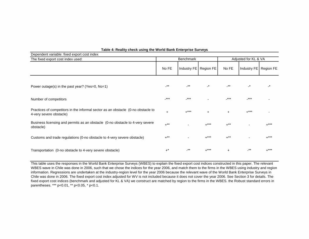
The fixed export cost index used:
No FE Industry FE Region FE No FE Industry FE Region FE
Power outage(s) in the past year? (Yes=0, No=1) -** -** -* -** -* -*
Number of competitors -*** -*** - -*** -*** -
Practices of competitors in the informal sector as an obstacle (0-no obstacle to
4-very severe obstacle) + +*** + + +*** -
Business licensing and permits as an obstacle (0-no obstacle to 4-very severe
obstacle) +** - +*** +** - +***
Customs and trade regulations (0-no obstacle to 4-very severe obstacle) +** - +*** +** - +***
Transportation (0-no obstacle to 4-very severe obstacle) +* -** +*** + -** +***
Benchmark Adjusted for KL & VA
Table 4: Reality check using the World Bank Enterprise Surveys
Dependent variable: fixed export cost index
This table uses the responses in the World Bank Enterprise Surveys (WBES) to explain the fixed export cost indices constructed in this paper. The relevant
WBES wave in Chile was done in 2006, such that we chose the indices for the year 2006, and match them to the firms in the WBES using industry and region
information. Regressions are undertaken at the industry-region level for the year 2006 because the relevant wave of the World Bank Enterprise Surveys in
Chile was done in 2006. The fixed export cost index adjusted for WV is not included because it does not cover the year 2006. See Section 3 for details. The
fixed export cost indices (benchmark and adjusted for KL & VA) we construct are matched by region to the firms in the WBES. the Robust standard errors in
parentheses. *** p<0.01, ** p<0.05, * p<0.1.

(1) (2) (3) (4) (5) (6)
Fixed export cost index Lagged benchmark Adjusted for KL & VA Adjusted for WV
Fixed export costs (f) -0.064*** -0.057*** -0.065*** -0.061*** -0.067*** -0.038**
(0.016) (0.015) (0.017) (0.020) (0.018) (0.018)
lnTFP 0.246*** 0.263*** 0.264*** 0.238*** 0.264*** 0.320***
(0.022) (0.021) (0.022) (0.024) (0.022) (0.034)
Capital-Labor ratio (KL) 0.039 0.045 -0.002 0.046 0.114
(0.074) (0.074) (0.073) (0.075) (0.151)
Value-added ratio (VA) -0.834*** -0.003* -0.003 -0.003* -0.002
(0.075) (0.002) (0.002) (0.002) (0.003)
Tariff rate -0.832*** -0.860*** -0.833*** -0.681***
(0.076) (0.088) (0.076) (0.098)
Crime rate -0.009 -0.010 -0.009 -0.007
(0.008) (0.010) (0.008) (0.012)
Mortality rate 0.005 0.007 0.009 0.052
(0.022) (0.025) (0.022) (0.034)
Constant -1.833*** -1.025*** -0.993*** -0.846** -1.007*** -2.067***
(0.319) (0.191) (0.305) (0.343) (0.307) (0.638)
Observations 20,271 20,271 20,271 15,184 20,271 11,783
Industry and year fixed effects are included. Robust standard errors in parentheses. *** p<0.01, ** p<0.05, * p<0.1.
Table 5: Export decisions, Fixed Export Costs, and Productivity
Dependent variable: export decision
Benchmark

Fixed export cost index
P(X=1) dP(X=1)/df f P(X=1) dP(X=1)/df f P(X=1) dP(X=1)/df f
25th percentile 0.17 -0.014 3.198 0.17 -0.015 3.307 0.16 -0.007 3.648
Median 0.16 -0.014 3.998 0.16 -0.014 4.100 0.16 -0.007 4.479
75th percentile 0.15 -0.013 4.788 0.15 -0.014 4.853 0.15 -0.007 5.218
From 25th to 75th 0.02 -0.001 -1.590 0.02 -0.001 -1.546 0.01 0.000 -1.571
Adjusted for WV
Table 6: Marginal effects of fixed export costs
The three groups correspond to, respectively, columns (3), (5), and (6) in Table 5.
Adjusted for KL & VABenchmark
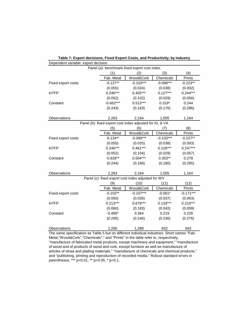
(1) (2) (3) (4)
Fab. Metal Wood&Cork Chemicals Prints
Fixed export costs -0.127** -0.103*** -0.098*** -0.223**
(0.055) (0.024) (0.038) (0.092)
lnTFP 0.246*** 0.455*** 0.127*** 0.244***
(0.052) (0.102) (0.029) (0.056)
Constant -0.662*** 0.513*** 0.319* 0.244
(0.243) (0.163) (0.176) (0.286)
Observations 2,263 2,164 1,505 1,164
(5) (6) (7) (8)
Fab. Metal Wood&Cork Chemicals Prints
Fixed export costs -0.134** -0.099*** -0.103*** -0.227**
(0.055) (0.025) (0.038) (0.093)
lnTFP 0.246*** 0.461*** 0.126*** 0.247***
(0.052) (0.104) (0.029) (0.057)
Constant -0.628** 0.504*** 0.353** 0.278
(0.244) (0.166) (0.180) (0.295)
Observations 2,263 2,164 1,505 1,164
(9) (10) (11) (12)
Fab. Metal Wood&Cork Chemicals Prints
Fixed export costs -0.102** -0.107*** -0.061* -0.171***
(0.050) (0.035) (0.037) (0.063)
lnTFP 0.213*** 0.679*** 0.133*** 0.210***
(0.060) (0.183) (0.042) (0.059)
Constant -0.490* 0.364 0.219 0.228
(0.295) (0.246) (0.236) (0.276)
Observations 1,280 1,288 832 642
Table 7: Export decisions, Fixed Export Costs, and Productivity, by industry
Dependent variable: export decision
Panel (a): benchmark fixed export cost index
Panel (b): fixed export cost index adjusted for KL & VA
Panel (c): fixed export cost index adjusted for WV
The same specification as Table 5 but on different individual industries. Short names "Fab.
Metal,"Wood&Cork","Chemicals"," and "Prints" in the table refer to, respectively,
"manufacture of fabricated metal products, except machinery and equipment," "manufacture
of wood and of products of wood and cork, except furniture as well as manufacture of
articles of straw and plaiting materials," "manufacture of chemicals and chemical products,"
and "publishing, printing and reproduction of recorded media." Robust standard errors in
parentheses. *** p<0.01, ** p<0.05, * p<0.1.
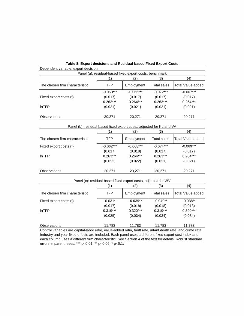
(1) (2) (3) (4)
The chosen firm characteristic TFP Employment Total sales Total Value added
-0.060*** -0.066*** -0.072*** -0.067***
Fixed export costs (f) (0.017) (0.017) (0.017) (0.017)
0.262*** 0.264*** 0.263*** 0.264***
lnTFP (0.021) (0.021) (0.021) (0.021)
Observations 20,271 20,271 20,271 20,271
(1) (2) (3) (4)
The chosen firm characteristic TFP Employment Total sales Total Value added
Fixed export costs (f) -0.062*** -0.068*** -0.074*** -0.069***
(0.017) (0.018) (0.017) (0.017)
lnTFP 0.263*** 0.264*** 0.263*** 0.264***
(0.022) (0.022) (0.021) (0.021)
Observations 20,271 20,271 20,271 20,271
(1) (2) (3) (4)
The chosen firm characteristic TFP Employment Total sales Total Value added
Fixed export costs (f) -0.031* -0.039** -0.040** -0.038**
(0.017) (0.018) (0.018) (0.018)
lnTFP 0.319*** 0.320*** 0.319*** 0.320***
(0.035) (0.034) (0.034) (0.034)
Observations 11,783 11,783 11,783 11,783
Control variables are capital-labor ratio, value-added ratio, tariff rate, infant death rate, and crime rate.
Industry and year fixed effects are included. Each panel uses a different fixed export cost index and
each column uses a different firm characteristic. See Section 4 of the text for details. Robust standard
errors in parentheses. *** p<0.01, ** p<0.05, * p<0.1.
Table 8: Export decisions and Residual-based Fixed Export Costs
Dependent variable: export decision
Panel (a): residual-based fixed export costs, benchmark
Panel (b): residual-based fixed export costs, adjusted for KL and VA
Panel (c): residual-based fixed export costs, adjusted for WV
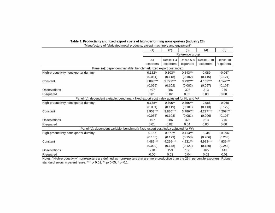
(1) (2) (3) (4) (5)
All
exporters
Decile 1-4
exporters
Decile 5-8
exporters
Decile 9-10
exporters
Decile 10
exporters
High-productivity nonexporter dummy 0.182** 0.303** 0.343*** -0.089 -0.067
(0.081) (0.118) (0.102) (0.115) (0.124)
Constant 3.893*** 3.772*** 3.732*** 4.163*** 4.142***
(0.055) (0.102) (0.082) (0.097) (0.108)
Observations 497 286 326 313 276
R-squared 0.01 0.02 0.03 0.00 0.00
High-productivity nonexporter dummy 0.188** 0.305** 0.355*** -0.086 -0.068
(0.081) (0.119) (0.101) (0.113) (0.122)
Constant 3.953*** 3.836*** 3.786*** 4.227*** 4.209***
(0.055) (0.103) (0.081) (0.096) (0.106)
Observations 497 286 326 313 276
R-squared 0.01 0.02 0.04 0.00 0.00
High-productivity nonexporter dummy 0.157 0.377** 0.413*** -0.34 -0.296
(0.135) (0.179) (0.158) (0.206) (0.263)
Constant 4.486*** 4.266*** 4.231*** 4.983*** 4.939***
(0.090) (0.148) (0.121) (0.180) (0.243)
Observations 278 153 180 165 141
R-squared 0.00 0.03 0.04 0.02 0.01
Notes: "High-productivity" nonexporters are defined as nonexporters that are more productive than the 25th percentile exporters. Robust
standard errors in parentheses. *** p<0.01, ** p<0.05, * p<0.1.
Panel (c): dependent variable: benchmark fixed export cost index adjusted for WV
Table 9: Productivity and fixed export costs of high-performing nonexporters (industry 28)
Reference group
Panel (a): dependent variable: benchmark fixed export cost index
Panel (b): dependent variable: benchmark fixed export cost index adjusted for KL and VA
“Manufacture of fabricated metal products, except machinery and equipment”
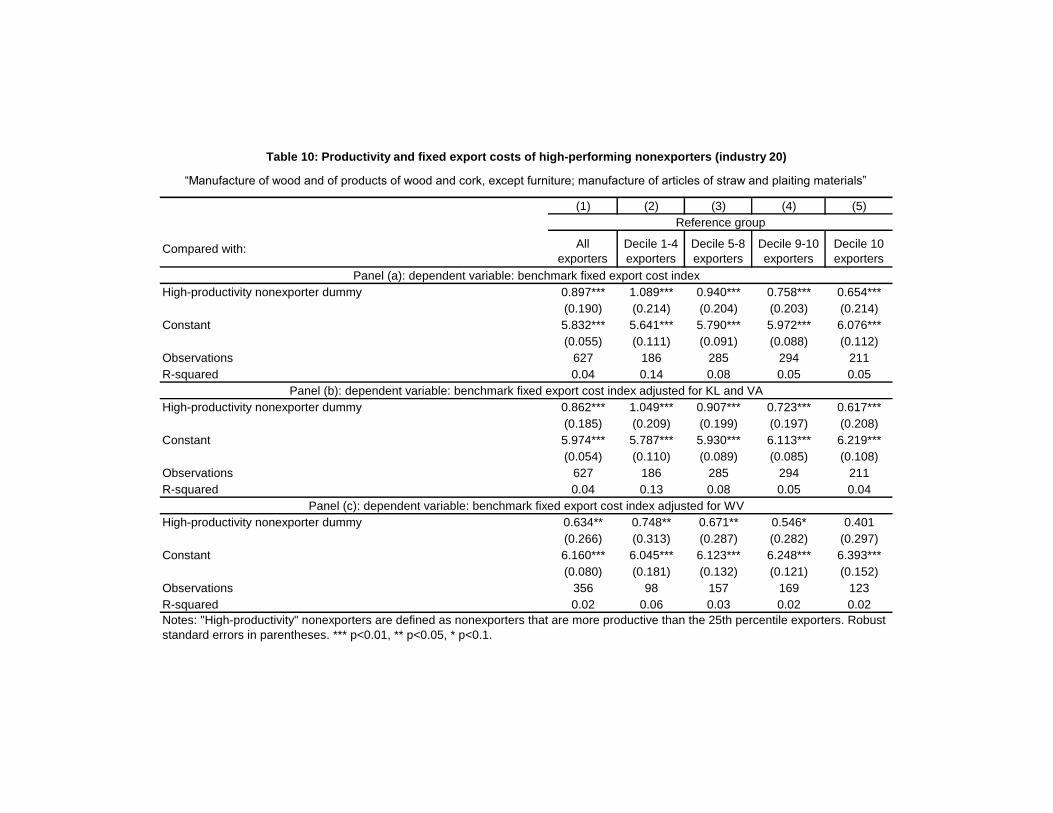
(1) (2) (3) (4) (5)
Compared with: All
exporters
Decile 1-4
exporters
Decile 5-8
exporters
Decile 9-10
exporters
Decile 10
exporters
High-productivity nonexporter dummy 0.897*** 1.089*** 0.940*** 0.758*** 0.654***
(0.190) (0.214) (0.204) (0.203) (0.214)
Constant 5.832*** 5.641*** 5.790*** 5.972*** 6.076***
(0.055) (0.111) (0.091) (0.088) (0.112)
Observations 627 186 285 294 211
R-squared 0.04 0.14 0.08 0.05 0.05
High-productivity nonexporter dummy 0.862*** 1.049*** 0.907*** 0.723*** 0.617***
(0.185) (0.209) (0.199) (0.197) (0.208)
Constant 5.974*** 5.787*** 5.930*** 6.113*** 6.219***
(0.054) (0.110) (0.089) (0.085) (0.108)
Observations 627 186 285 294 211
R-squared 0.04 0.13 0.08 0.05 0.04
High-productivity nonexporter dummy 0.634** 0.748** 0.671** 0.546* 0.401
(0.266) (0.313) (0.287) (0.282) (0.297)
Constant 6.160*** 6.045*** 6.123*** 6.248*** 6.393***
(0.080) (0.181) (0.132) (0.121) (0.152)
Observations 356 98 157 169 123
R-squared 0.02 0.06 0.03 0.02 0.02
Notes: "High-productivity" nonexporters are defined as nonexporters that are more productive than the 25th percentile exporters. Robust
standard errors in parentheses. *** p<0.01, ** p<0.05, * p<0.1.
Panel (c): dependent variable: benchmark fixed export cost index adjusted for WV
Table 10: Productivity and fixed export costs of high-performing nonexporters (industry 20)
Reference group
Panel (a): dependent variable: benchmark fixed export cost index
Panel (b): dependent variable: benchmark fixed export cost index adjusted for KL and VA
“Manufacture of wood and of products of wood and cork, except furniture; manufacture of articles of straw and plaiting materials”

Dependent variable: firm-level export volume
(1) (2) (3) (4) (5) (6) (7) (8) (9) (10)
Measure of fixed export costs
Dependent variable ln(V+1) Pr(X=1) ln(V+1) Pr(X=1) ln(V+1) Pr(X=1) ln(V+1) Pr(X=1) ln(V+1) Pr(X=1)
Fixed export costs 0.053 -0.049*** 0.042 -0.053*** 0.033 -0.052*** 0.045 -0.055*** -0.028 -0.028*
(0.066) (0.015) (0.061) (0.018) (0.068) (0.020) (0.062) (0.018) (0.062) (0.017)
lnTFP 0.749*** 0.192*** 0.840*** 0.230*** 0.787*** 0.215*** 0.840*** 0.230*** 0.911*** 0.249***
(0.073) (0.018) (0.065) (0.020) (0.073) (0.023) (0.065) (0.020) (0.085) (0.027)
Constant 10.821*** -1.046*** 10.199*** -0.613*** 9.366*** -0.577** 10.201*** -0.622*** 10.546*** -1.040***
(0.479) (0.085) (0.776) (0.209) (0.900) (0.245) (0.775) (0.209) (0.998) (0.295)
Athrho & lnsigma 0.298*** 0.888*** 0.192*** 0.793*** 0.224*** 0.784*** 0.193*** 0.793*** 0.230*** 0.817***
(0.056) (0.020) (0.043) (0.016) (0.046) (0.019) (0.043) (0.016) (0.069) (0.020)
Firm-level control variables No No Yes Yes Yes Yes Yes Yes Yes Yes
Observations 20,271 20,271 20,271 20,271 15,184 15,184 20,271 20,271 11,783 11,783
Benchmark Adjusted for WV
Table 11: Fixed export costs and export volume
Control variables are capital-labor ratio, value-added ratio, tariff rate, infant death rate, and crime rate. Industry and year fixed effects are included. Robust
standard errors in parentheses. *** p<0.01, ** p<0.05, * p<0.1.
Adjusted for KL & VALagged benchmark

Dependent variable: export decision
(1) (2) (3) (4) (5) (6) (7) (8)
Lagged
benchmark
Adjusted for
KL & VA
Adjusted for
WVUsing lnTFP
Using
lnTFP
percentile
Fixed export costs (f) -0.149*** -0.147*** -0.132*** -0.146*** -0.128*** -0.087*** -0.087*** -0.208***
(0.021) (0.022) (0.025) (0.022) (0.025) (0.021) (0.021) (0.027)
lnTFP 0.039 0.084*** 0.072*** 0.085*** 0.103*** 0.101*** -0.083 -0.019
(0.026) (0.023) (0.026) (0.023) (0.034) (0.030) (0.051) (0.027)
Fixed export costs x 0.056*** 0.058*** 0.052*** 0.056*** 0.065***
productivity quarter 2 (0.011) (0.010) (0.011) (0.010) (0.014)
Fixed export costs x 0.114*** 0.108*** 0.092*** 0.105*** 0.123***
productivity quarter 3 (0.014) (0.013) (0.014) (0.013) (0.018)
Fixed export costs x 0.146*** 0.133*** 0.117*** 0.129*** 0.144***
productivity quarter 4 (0.019) (0.017) (0.018) (0.017) (0.023)
Fixed export costs quarter 2 x 0.107**
productivity (0.045)
Fixed export costs quarter 2 x 0.284***
productivity (0.062)
Fixed export costs quarter 2 x 0.403***
productivity (0.071)
Fixed export costs x 0.088***
productivity (0.015)
Fixed export costs x 0.256***
productivity percentile within industry-year (0.028)
Constant -1.797*** -1.031*** -0.799** -1.038*** -2.103*** -1.721*** -1.369*** -1.126***
(0.311) (0.316) (0.336) (0.317) (0.649) (0.622) (0.472) (0.334)
Control variables No Yes Yes Yes Yes Yes Yes Yes
Observations 20,271 20,271 15,184 20,271 11,783 20,271 20,271 20,271
Control variables are capital-labor ratio, value-added ratio, tariff rate, infant death rate, and crime rate. Industry and year fixed effects are included. Robust
standard errors in parentheses. *** p<0.01, ** p<0.05, * p<0.1.
Benchmark
Table 12: Interaction between fixed export costs and productivity
Different fixed export cost indices
Symmetric
effects
Single interaction
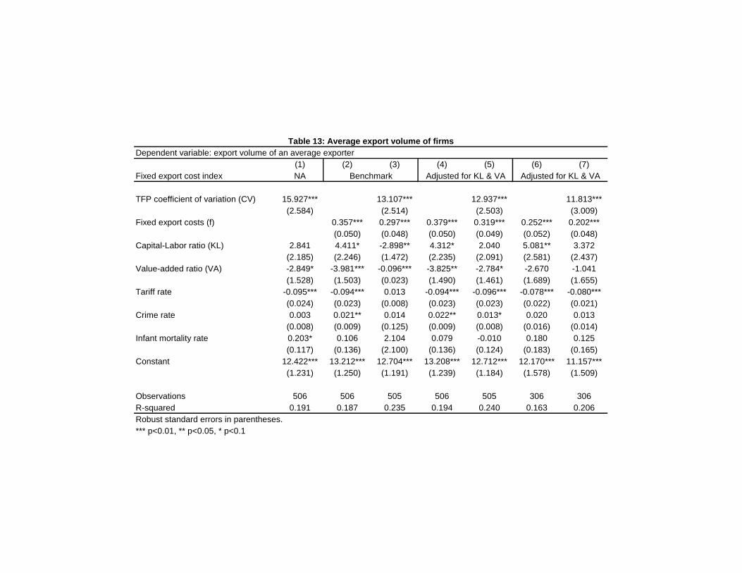
(1) (2) (3) (4) (5) (6) (7)
Fixed export cost index NA
TFP coefficient of variation (CV) 15.927*** 13.107*** 12.937*** 11.813***
(2.584) (2.514) (2.503) (3.009)
Fixed export costs (f) 0.357*** 0.297*** 0.379*** 0.319*** 0.252*** 0.202***
(0.050) (0.048) (0.050) (0.049) (0.052) (0.048)
Capital-Labor ratio (KL) 2.841 4.411* -2.898** 4.312* 2.040 5.081** 3.372
(2.185) (2.246) (1.472) (2.235) (2.091) (2.581) (2.437)
Value-added ratio (VA) -2.849* -3.981*** -0.096*** -3.825** -2.784* -2.670 -1.041
(1.528) (1.503) (0.023) (1.490) (1.461) (1.689) (1.655)
Tariff rate -0.095*** -0.094*** 0.013 -0.094*** -0.096*** -0.078*** -0.080***
(0.024) (0.023) (0.008) (0.023) (0.023) (0.022) (0.021)
Crime rate 0.003 0.021** 0.014 0.022** 0.013* 0.020 0.013
(0.008) (0.009) (0.125) (0.009) (0.008) (0.016) (0.014)
Infant mortality rate 0.203* 0.106 2.104 0.079 -0.010 0.180 0.125
(0.117) (0.136) (2.100) (0.136) (0.124) (0.183) (0.165)
Constant 12.422*** 13.212*** 12.704*** 13.208*** 12.712*** 12.170*** 11.157***
(1.231) (1.250) (1.191) (1.239) (1.184) (1.578) (1.509)
Observations 506 506 505 506 505 306 306
R-squared 0.191 0.187 0.235 0.194 0.240 0.163 0.206
*** p<0.01, ** p<0.05, * p<0.1
Robust standard errors in parentheses.
Table 13: Average export volume of firms
Dependent variable: export volume of an average exporter
Benchmark Adjusted for KL & VA Adjusted for KL & VA
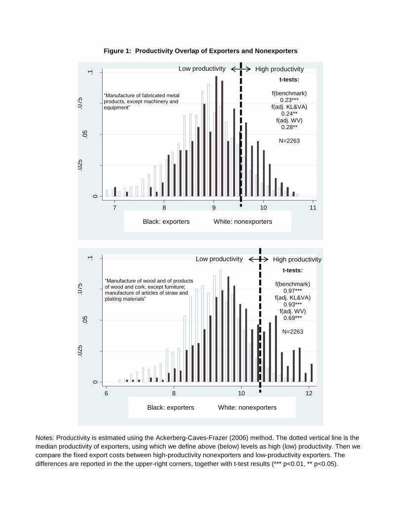
Figure 1: Productivity Overlap of Exporters and Nonexporters
Notes: Productivity is estmated using the Ackerberg-Caves-Frazer (2006) method. The dotted vertical line is the
median productivity of exporters, using which we define above (below) levels as high (low) productivity. Then we
compare the fixed export costs between high-productivity nonexporters and low-productivity exporters. The
differences are reported in the the upper-right corners, together with t-test results (*** p<0.01, ** p<0.05).
0
.025
.05
.075
.1
Fra
ction
7 8 9 10 11lntfp
0 1
0
.025
.05
.075
.1
Fra
ction
6 8 10 12lntfp
0 1
Black: exporters White: nonexporters
“Manufacture of fabricated metal products, except machinery and equipment”
“Manufacture of wood and of products of wood and cork, except furniture; manufacture of articles of straw and plaiting materials”
Black: exporters White: nonexporters
High productivity
Low productivity High productivity
Low productivity
t-tests:
f(benchmark)
0.23*** f(adj. KL&VA)
0.24** f(adj. WV)
0.28**
N=2263
t-tests:
f(benchmark)
0.97*** f(adj. KL&VA)
0.93*** f(adj. WV)
0.69***
N=2263
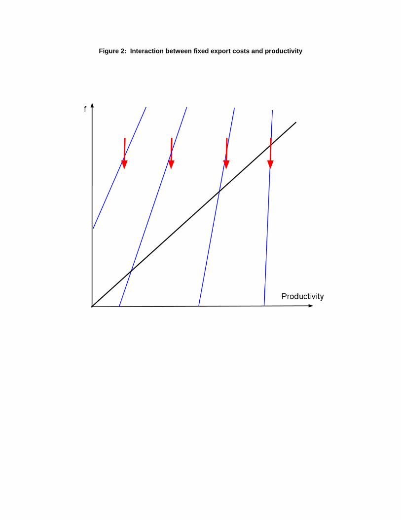
Figure 2: Interaction between fixed export costs and productivity

Figure 3: Maps of Chile
Left: administrative regions Middle: seaports Right: airports

Figure 4: Residuals from the first step regression
0
.05
.1.1
5
Density
-10 -5 0 5 10 15Residuals
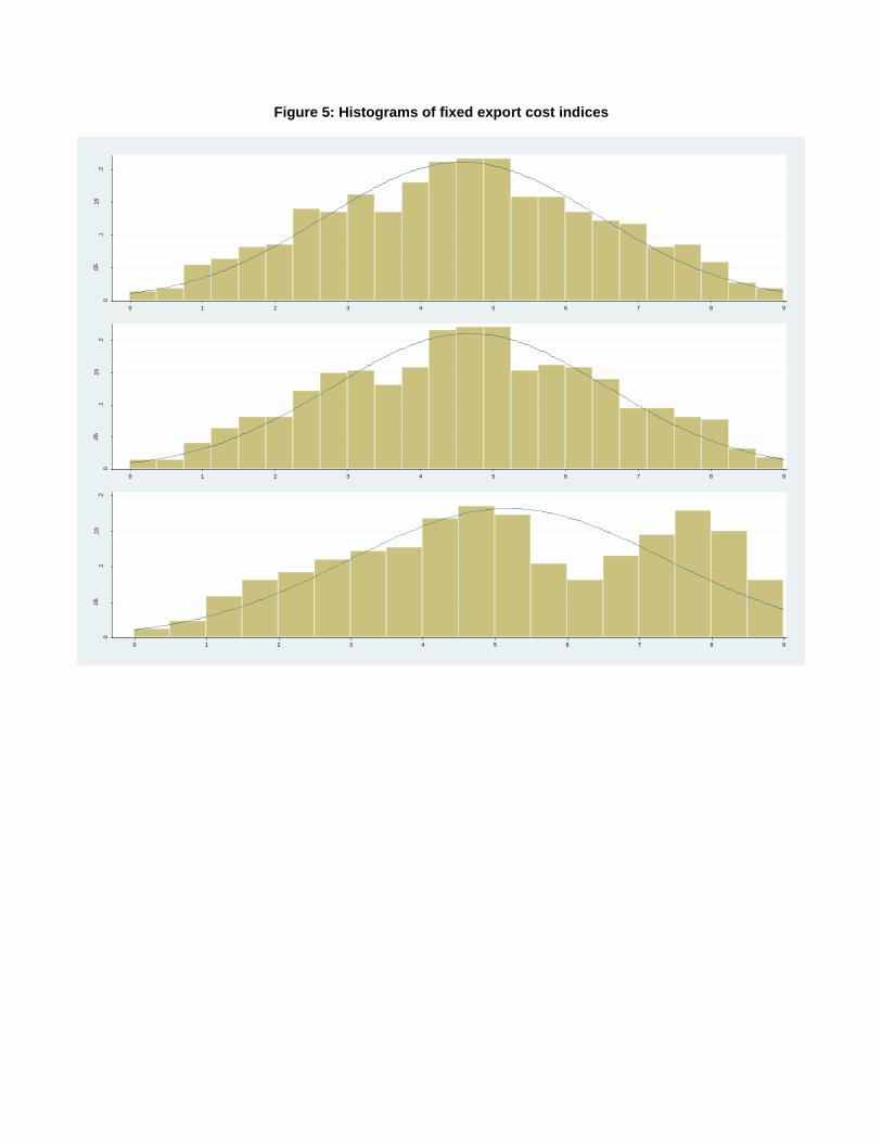
Figure 5: Histograms of fixed export cost indices
0
.05
.1.1
5.2
Den
sity
0 1 2 3 4 5 6 7 8 9
0
.05
.1.1
5.2
Den
sity
0 1 2 3 4 5 6 7 8 9
0
.05
.1.1
5.2
Den
sity
0 1 2 3 4 5 6 7 8 9

Figure 6: Fixed export costs along three dimensions
Panel (a): By industry
Panel (b): By region
0 2 4 6 8
WoodOther transport
Machinery and equipmentBasic metals
ChemicalsPaper
Rubber and plastics productsFabricated metal products
ApparelTextiles
Motor vehiclesPublishing
Precision instrumentsLeather
Non-metallic mineral productsElectrical machinery
FurnitureCommunication equipment
25th and 75th percentiles, by industry
25th percentile 75th percentile
0 2 4 6 8
Maule
Araucania
Gral. Bernardo O'Higgins
Los Lagos
Magallanes y de la Antártica Chilena
Valparaiso
Antofagasta
Biobio
Atacama
Metropolitana de Santiago
General Carlos Ibanez del Campo
Coquimbo
Tarapaca
25th and 75th percentiles, by region
25th percentile 75th percentile

Figure 6: Fixed export costs along three dimensions (cont’d)
Panel (c): By year
0 2 4 6
2007
2006
2005
2004
2003
2002
2001
25th and 75th percentiles, by year
25th percentile 75th percentile

YearsTotal No.
of firms
No. of new
exporters
Share of new
exporters
No. of new
quitters
Share of new
quitters
No. of new
exporters who are
also quitters
Share of new
exporters who are
also quitters
2001 2,739 NA NA 96 3.50% NA NA
2002 2,987 47 1.57% 49 1.64% 27 0.90%
2003 2,987 44 1.47% 61 2.04% 38 1.27%
2004 3,070 33 1.07% 39 1.27% 35 1.14%
2005 2,985 38 1.27% 37 1.24% 43 1.44%
2006 2,846 24 0.84% 40 1.41% 32 1.12%
2007 2,660 19 0.71% NA NA NA NA
Average 2,896 34.17 1.16% 54 1.85% 35 1.21%
Table A1: New Exporters and Quitters
This table summaries number and share of new exporters, which are defined as firms that export in the current year but not the
previous year. As a comparison, it also reports counterpart statistics of quitters, defined as firms that export in the current year but
not the next year. Since our data cover years 2001—2007, information on new exporters in 2001 and quitters in 2007 are
unavailable.
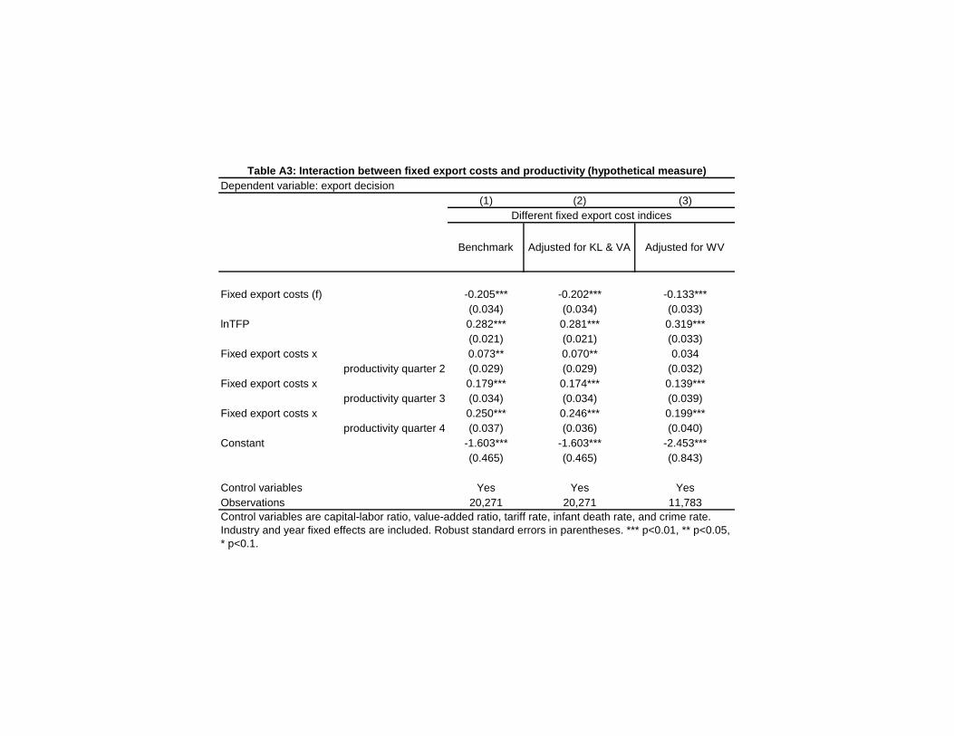
Dependent variable: export decision
(1) (2) (3)
Benchmark Adjusted for KL & VA Adjusted for WV
Fixed export costs (f) -0.205*** -0.202*** -0.133***
(0.034) (0.034) (0.033)
lnTFP 0.282*** 0.281*** 0.319***
(0.021) (0.021) (0.033)
Fixed export costs x 0.073** 0.070** 0.034
productivity quarter 2 (0.029) (0.029) (0.032)
Fixed export costs x 0.179*** 0.174*** 0.139***
productivity quarter 3 (0.034) (0.034) (0.039)
Fixed export costs x 0.250*** 0.246*** 0.199***
productivity quarter 4 (0.037) (0.036) (0.040)
Constant -1.603*** -1.603*** -2.453***
(0.465) (0.465) (0.843)
Control variables Yes Yes Yes
Observations 20,271 20,271 11,783
Table A3: Interaction between fixed export costs and productivity (hypothetical measure)
Different fixed export cost indices
Control variables are capital-labor ratio, value-added ratio, tariff rate, infant death rate, and crime rate.
Industry and year fixed effects are included. Robust standard errors in parentheses. *** p<0.01, ** p<0.05,
* p<0.1.

(1) (2) (3)
Estimation method OLS
Dependent variable ln(V+1) ln(V+1) Pr(X=1)
Fixed export costs 0.136*** 0.229*** -0.050***
(0.049) (0.068) (0.016)
Constant 9.531*** 14.314*** -0.840***
(0.856) (0.917) (0.201)
Athrho & lnsigma -1.326*** 1.270***
(0.088) (0.042)
Control variables Yes Yes Yes
Observations 3,701 20,271 20,271
Table A4: Fixed export costs and export volume, without controlling for productivity
Column (1) includes only exporters. Columns (2) and (3) include all firms, and are jointly
estimated to correct the truncation in firm-level export volume. Control variables are capital-
labor ratio, value-added ratio, tariff rate, crime rate, and infant mortality. Industry and year
fixed effects are included. Robust standard errors in parentheses. *** p<0.01, ** p<0.05, *
p<0.1.
Tobit II
The dependent variable: firm-level export volume


