1

Identifying Biomass Burning Emission Differences Between NH3

& CO using 13 years of AIRS Satellite Measurements

Ashley A. Wheeler A scholarly paper in partial fulfillment of the requirements for the degree of

Master of Science

December 2016

Department of Atmospheric and Oceanic Science, University of Maryland

College Park, Maryland

Advisor: Dr. Juying Warner

2

Table of Contents

Acknowledgements

List of Tables

List of figures

List of symbols

Chapter 1. Introduction

1.1 NASA Earth Observing System (EOS)

1.2 Aqua Satellite and AIRS Instrumentation

1.3 Atmospheric Ammonia; Importance, Modeling, and Satellite Observations

1.4 Atmospheric Carbon Monoxide; Importance and Satellite Observations

1.5 MODIS Fire Radiative Power

Chapter 2. Data Sets & Methods

2.1 Brief Retrieval Method Overview

2.2 Data Sets

2.3 Calculations

Chapter 3. Results

3.1 NH3 and CO Global Distributions, Seasonal Correlation, & Relative Emissions Ratio

3.2 Identifying Fire Regions Using a “Threshold”

3.3 Regional Time Series of NH3, CO, and MODIS Total Fire Counts

Chapter 4. Conclusions & Summary

References

3

Acknowledgements

I would like to thank my graduate advisor Dr. Juying Warner for her

encouragement, support, and guidance throughout my academic career at the University

of Maryland. Dr. Warner’s passion for her research. It was a privilege to work with and

learn from Dr. Warner, her enthusiasm for research is contagious.

I am forever thankful for the love and support of my parents, Anne and Brian

Wheeler, and my brother Matthew. Without them I could not have made it this far. I

would also like to thank my Grandfather, Fredrick Brooks, for inspiring me since a young

age to love science and pursue big dreams. I would also like to thank the AOSC faculty

and my fellow peers for enjoying this journey with me.

I am forever thankful for the love and support of my family. To my parents Anne

and Brian Wheeler; Thank you for providing me with the opportunities that allowed me

to reach this point as well as for your patience, reassurance, and understanding along the

way. To my brother Matthew; Thank you for always believing in me and challenging me

to be better. To my Grandfather Fredrick Brooks; Thank you for continuously inspiring

me since a young age to love science and pursue big dreams. Without you all, I could not

have made it this far.

Finally, thank you to all my friends, teammates, and coaches who have

encouraged me to follow my passion. I am truly grateful for all those who have helped

me and been a part of my career thus far.

Thank you!

Ashley

4

List of Tables

Table 1. Min/Max Latitude & Longitude Bounds of 6 Fire Regions

5

List of Figures Figure 1. A-Train Satellite Configuration

2. IDL Example Code Demo. of “WHERE” Function Matching

3. AIRS 505mb CO VMRs for Each Season Averaged over 2003-2015

4. AIRS 918mb NH3 VMRs for Each Season Averaged over 2003-2015

5. Multi-Panel Plot for Summer from 2003-2015 TOP LEFT: AIRS L2V6 500 mb CO VMR BOTTOM LEFT: AIRS L2V6 918 mb NH3 VMR TOP RIGHT: NH3 vs CO Correlation Coefficient BOTTOM RIGHT: NH3 to CO Relative Emission Ratio

6. Multi-Panel Plot for Spring from 2003-2015 TOP LEFT: AIRS L2V6500 mb CO VMR BOTTOM LEFT: AIRS L2V6 918 mb NH3 VMR TOP RIGHT: NH3 vs CO Correlation Coefficient BOTTOM RIGHT: NH3 to CO Relative Emission Ratio

7. Screened Multi-Panel Plot for Summer from 2003-2015 TOP LEFT: MODIS Total Fire Counts BOTTOM LEFT: MODIS Fire Radiative Power TOP RIGHT: Screened NH3 vs CO Correlation Coefficient. BOTTOM RIGHT: Screened NH3 to CO Relative Emission Ratio

8. Screened Multi-Panel Plot for Spring from 2003-2015 TOP LEFT: MODIS Total Fire Counts BOTTOM LEFT: MODIS Fire Radiative Power TOP RIGHT: Screened NH3 vs CO Correlation Coefficient. BOTTOM RIGHT: Screened NH3 to CO Relative Emission Ratio

6

9. Map of 6 Fire Regions of Interest

10a. Regional Time Series of AIRS NH3 and CO VMR with Total MODIS Fire Counts from 2003-2015

REGIONS: Africa North of Equator, Africa South of Equator Central South America, and South East Asia 10b. Regional Time Series of AIRS NH3 and CO VMR with

Total MODIS Fire Counts from 2003-2015 REGIONS: Alaska/CA, Russia

7

List of Acronyms

AIRS

EOS

ESE

NASA

HCl

HNO3

H2SO4

SOA

MODIS

FRP

mb

NH3

CO

VMR

OE

Atmospheric Infrared Sounder

Earth Observing System

Earth Science Enterprise

National Aeronautics and Space Administration

Hydrochloric Acid

Nitric Acid

Sulfuric Acid

Secondary Organic Aerosols

MODerate Resolution Imaging Spectroradiometer

Fire Radiative Power

Millibar

Ammonia

Carbon Monoxide

Volume Mixing Ratio

Optimal Estimation

8

Chapter 1. Introduction

1.1 NASA Earth Observing System (EOS) In the 1990s NASA’s Earth Observing System (EOS) Program was founded as a part of the

Earth Science Enterprise (ESE) in response to the growing recognition of societies impact

on the natural variability and evolution of the planet. Following the discovery of the ozone

hole over Antarctica, increasing carbon dioxide concentrations recorded at Mauna Loa,

observed tropical deforestation, and global warming patterns predicted by climate models,

there was a sense of urgency to understand the entire Earth system on a global scale. The

overall goal of the EOS Program is “to advance the understanding of the entire Earth

system on a global scale by improving our knowledge of the components of the system, the

interactions between them, and how the Earth system is changing” (NASA, 1999). The

EOS is composed of a series of coordinated polar-orbiting satellites producing long-term

global observations used to understand critical aspects Earth’s climate system, including;

greenhouse gases, radiation, land and sea ice, clouds, ozone, the oceans, both natural and

anthropogenic aerosols, precipitation, etc. As a part the Earth Science Division of NASA’s

Science Mission Directorate, the original EOS Program has been involved in international

and multidisciplinary collaborations that lead to countless scientific discoveries studying

the atmosphere, ocean, biosphere, cryosphere, land surface, and the relationships between

them.

1.2 Aqua Satellite and AIRS Instrumentation

Terra (formally AM-1) launched in 1999 as the first Earth Observing System satellite,

collecting multiple types of data and becoming the first satellite to look at Earth system

9

science. Shortly following in 2002 was the launch Aqua (formerly EOS PM), the first of

NASA’s satellites that would make up the Afternoon Constellation or the A-Train. The A-

train is a group of satellites overseen by NASA and international associates that closely

follow each other in the same polar orbital track. Flying in a frozen sun-synchronous orbit,

the satellites cross the equator at an altitude of roughly 705 km (Demarest et al., 2005). The

six satellites currently in the A-Train: Orbiting Carbon Observatory (OCO-2), the Global

Change Observation Mission-Water (GCOM-W1), Aqua, Cloud-Aerosol Lidar and

Infrared Pathfinder Satellite Observation (CALIPSO), CloudSat, and Aura. See Figure 1 for

illustration of A-Train satellite configuration.

Figure 1. The Afternoon Constellation (from right to left) OCO-2, GCOM-W1, Aqua, CALIPSO, CloudSat, and Aura. The convoy formation of the six satellites allows for near-simultaneous measurements as

they pass a given target within seconds to minutes within each other (Schoeberl et al.,

2004). Multisensor observations from the satellites collectively produce a thorough vertical

3-D image of the atmosphere in various wavelengths and desirable climate parameters.

10

Aqua currently has 5 of its original six instruments working operationally: AIRS, AMSU,

CERES, MODIS, and AMSR-E. For the purpose of this study, AIRS will be the primary

instrument of interest.

The Atmospheric Infrared Sounder (AIRS) is cross-track scanning instrument designed to

measure the water vapor content and temperature profiles of the Earth’s atmosphere. The

high spectral resolution grating spectrometer has 2378 bands in the thermal infrared from

3.7 to 15.4 µm and 4 in the visible from 0.4 to 1.0 µm. The spectral ranges have been

precisely chosen in order for an accuracy of 1 K per 1 km thick layer in the troposphere for

atmospheric temperature and 20% per 2 km thick layer in the lower troposphere for

moisture profiles (Aumann et al., 2003). AIRS scans a ±49.5 degree swath every 8/3

seconds, nadir and perpendicular to the flight path with 90 ground footprints per scan. Each

individual footprint contains a single spectrum with all 2378 spectral samples taken

simultaneously at a spatial resolution of 13.5 km (Aumann and Miller, 1995). Although

designed as a meteorological mission, AIRS hyperspectral properties enable the retrievals

for a number of atmospheric chemistry species or minor compositions.

1.3 Atmospheric Ammonia; Importance, Modeling, and Satellite Observations

During recent years, the interest in atmospheric ammonia (NH3) has increased due to its

role in global climate change and air quality, resulting in a range of studies. Ammonia is a

critical component of the atmosphere composition and is an important factor in the

acidification and eutrophication of ecosystems and determining the acidity of precipitation

(Aneja et al., 2001, 2008; Shukla and Sharma, 2010). In its gaseous phase NH3 is one of the

11

only, and the most dominant, alkaline species in the atmosphere and neutralizes acidic

species such as sulfuric acid (H2SO4), hydrochloric acid (HCl), and nitric acid (HNO3) into

ammonium salts (Behera and Sharma, 2010). Secondary pollutants including SO2, NOx,

volatile organic compounds (VOCs), and ammonia are precursors to particulate matter

(PM) formation which results in a significant portion of secondary particulate matter of

diameter less than 2.5 micrometers, classified as PM2.5 (Behera and Sharma, 2010, 2012;

Updyke et al., 2012). Fine particles are very concerning for human health because of their

ability to penetrate deeper into lungs and the particle composition which can be very toxic.

Compared to larger aerosols, PM2.5 particles remain suspended in the air for longer, travel

further distances, and are capable of reaching indoor settings much easier due to their

smaller size. PM2.5 has therefore been a chief index of PM exposure that is closely linked to

cardiovascular and pulmonary health effects (Brook et al., 2010; Pope et al., 2011; Pope

and Dockery, 2006). These ammonium nitrate and ammonium sulfate particles, formed

through the reaction of NH3 with nitric acid and sulfuric acid, can also have a significant

impact climate and the Earth’s radiative balance. The effects occur; 1) directly by scattering

and absorbing radiation, 2) indirectly by acting as cloud condensation nuclei (CCN) which

impacts cloud formation and cloud radiative properties such as cloud albedo, and 3)

contributes to absorption of solar radiation via formation of brown carbon through the

reaction of NH3 with secondary organic aerosols (SOA) (Abbatt et al., 2006; Adams et al.,

2001; IPCC, 2013; Langridge et al., 2012; Updyke et al., 2012).

Despite its importance NH3 is acknowledged as one of the most poorly quantified trace

gases and is responsible for some of the largest uncertainties in reactive nitrogen

12

atmospheric transport (Fowler et al., 2013; Galloway et al., 2008; Pinder et al., 2006;

Sutton et al., 2008). To understand better the magnitude, spatial, and seasonal variability of

NH3 emissions models have been used to estimate atmospheric ammonia concentrations as

well as atmospheric transport. However, it has been suggested that current models

generally tend to underestimate concentration most particularly in the Northern Hemisphere

which is largely industrialized (Heald et al., 2012). Globally there is a limited number of

ground-based sites, networks, or field campaigns taking routine measurements of NH3

concentrations making it increasingly difficult to determine the spatial and temporal

variability. Examples of such measurements include the US Ammonia Monitoring Network

(AMoN), DISCOVER-AQ, and the European Monitoring and Evaluation Programme

(EMEP). Even with sparse coverage the in-situ measurements can require expensive

equipment and instruments that do not always prove to be reliable or consistent. Despite the

increasing availability of airborne and ship campaign datasets, which provide important

information about the vertical profile of NH3 and measurements over water respectively,

these datasets only cover a short time period over small scales. Yet another downfall of in-

situ measurements is the underrepresentation of the Southern Hemisphere which contains

regions critical for understanding NH3 emissions on a global scale.

In contrast to other techniques, satellite remote sensing provides high spatial and temporal

resolution that can complement and filling the gap left by in-situ measurements. The first

satellite observations of lower tropospheric NH3 were made over Beijing, China using the

Tropospheric Emission Spectrometer (TES) aboard the Aura satellite (Beer et al., 2008).

The TES NH3 retrieval strategy was thoroughly explained by Shephard et al. (2011) who

13

concluded that TES retrievals are primarily sensitive to NH3 between 700 and 900 mb and

produced global maps from TES NH3. Utilizing their findings, Luo et al. (2015)

investigated the seasonal and global distributions and correlations of NH3 to CO from TES

satellite observations compared to GEOS-Chem model simulations for 2007 (Bey et al.,

2001). Ammonia was detected inside biomass burning plumes during August 2007 in

Greece within a spectra from the Infrared Atmospheric Sounder Interferometer (IASI)

aboard the European MetOP polar orbiting satellites (Coheur et al., 2009). Observations

from IASI enabled global daily monitoring due to a quick retrieval method, constructed

around calculation total column measurements from brightness temperature, leading to the

first global map of NH3 distributions (Clarisse et al., 2009). During a case study of the San

Joaquin Valley Clarisse et al. (2010) focused on the sensitivity and ability of infrared

instruments to probe the lower troposphere. Using a more refined algorithm they

determined that the peak sensitivity for NH3 is within the boundary layer and can be

measured in cases when thermal contrast is large between the surface and bottom of the

atmosphere and NH3 concentrations are high (Clarisse et al., 2010). Clarisse et al. (2010)

also examined instrument and measurement sensitivity for daytime versus nighttime as well

as for different seasons. Following this study the NH3 detection sensitivity and retrieval

from IASI has been continually improved, first by Walker et al. (2011) and then by Van

Damme et al. (2014, 2015). Shephard and Cady-Pereira (2015) have also observed

atmospheric NH3 using the Cross-track Infrared Sounder (CrIS) on the Suomi National

Polar-orbiting Partnership (NPP) satellite.

14

While the studies mentioned above have made immense contributions to furthering our

knowledge of the seasonal variation and spatial distribution of NH3 emissions large

uncertainties still exist. In a most recent study Warner et al. (2016) describes a new NH3

retrieval method for the Atmospheric Infrared Sounder (AIRS) aboard NASA’s EOS Aqua

satellite, producing a daily and global ammonia product spanning 14 years from September

2002 to August 2016. The dataset presented by Warner et al. (2016) is the longest NH3

record to data and will be critical to advancing our understanding of NH3 emissions as well

as the global nitrogen cycle. The 14-year dataset provided by Warner et al. (2016) was used

for the purposes of this study, and will be described in greater detail in “Chapter 2: Data

Sets & Methods” and for the remainder of the paper.

1.4 Atmospheric Carbon Monoxide: Importance and Satellite Observations

Since 2002 AIRS has been making global measurements of carbon monoxide (CO). Other

sensors have contributed to global CO measurements such as; the Measurement Of

Pollution In The Troposphere (MOPITT), the Tropospheric Emission Spectrometer (TES),

the Infrared Atmospheric Sounder Interferometer (IASI), and The Cross-track Infrared

Sensor (CrIS). It is critical to understand CO in the atmosphere since it has both direct and

indirect impact and can be oxidized to form carbon dioxide (CO2), a vital greenhouse gas.

Due to its tropospheric lifetime of around 1-3 months, CO can have effects at larger scales

and be used as a tracer for atmospheric motions (Badr and Probert, 1994). Global

measurements of CO are essential for atmospheric chemistry models and air quality health

assessments due to its influences as a major sink for hydroxyl (OH) and precursor for

15

tropospheric ozone and smog (Crutzen et al., 1979). It is also important to note that

emissions of CO from biomass burning challenges its anthropogenic emissions at 50/50 and

causes most of its interannually variability (van der Werf et al., 2006). For the purpose of

this study, CO and NH3 have overlapping emission sources from biomass burning including

wildfires and agricultural fires (Akagi et al., 2011) which will aid in determining origins of

the observed NH3 measurements.

1.5 MODIS Fire Radiative Power

The active fire products produced by NASA’s Moderate Resolution Imaging

Spetroradiometer (MODIS) provide important information that has been used in countless

biomass burning studies (Giglio et al., 2006; Justice et al., 2002). The active fires are

monitored and detected at a resolution of about 1 km using the 4 µm and 11 µm bands to

derive brightness temperatures (Justice et al., 2002). Fire Radiative Power (FRP), which is

derived from the 4 µm band, is the rate at which the actively burning fire is emitting

radiative energy, at the time of observation, expressed in units of power (Js-1 or Watts).

Wooster et al. (2005) linked FRP to combustion rate by showing the linear relationship

between the amount of biomass burned in a fire and the radiation released by the fire. From

this concept, we can use FRP to identify biomass burning regions and analyze NH3 and CO

emission ratios.

16

Chapter 2. Data Sets & Methods 2.1 Brief Retrieval Method Overview

The 13 year data set used during this study, spanning from 2003 through 2015, was

produced by a retrieval algorithm using an optimal estimation (OE) technique that was

developed by Warner et al. (2016). This AIRS NH3 retrieval algorithm was based off

AIRS carbon monoxide (CO) products established by Warner et al. (2010) and expanded

off the current AIRS operational system algorithm (Susskind et al., 2003) with the

exception of an alternate minimization method. It is important to note that AIRS data

coverage has been increased from pure clear the coverage of about 10-15%, to roughly

50-70% of total measurements at 13.5 km2 for a single pixel (Warner et al., 2013) as a

result of AIRS cloud clearing capabilities outlined in Susskind et al. (2003). To ensure

the greatest sensitivity to NH3, the retrievals were completed at 12 channels of AIRS

radiances within the window regions of 860-875, 928-932, and 965-967 cm-1.

For a more thorough and detailed account of the AIRS NH3 retrieval method please refer

to Warner et al. (2016).

2.2 Data Sets

This study exams various data sets over the time period of 13 years from 2002-2015. Both

the carbon monoxide and ammonia data sets used during this study were retrieved and

provided by Dr. Juying Warner using AIRS Level 2 Version 6 and OE method. The CO

data was provided in daily swath (240 granules per day) Hierarchical Data Format (HDF)

files (Warner et al., 2010), from which CO VMR at 505 mb was extracted. The NH3 VMR

data was obtained at 918 mb from daily Network Common Data Form (NetCDF) files

17

(Warner et al., 2016). As the AIRS NH3 was being read in, it was also screened to ensure

only the highest quality data with elevated emissions (NH3 VMR ≥ 1.0 ppbv) was kept. The

screening criteria includes;

1. AIRS CCR quality assurance flag = Q0 (Highest quality)

2. The degrees of freedom for signal (DOFS) provided by the OE retrieval

output must be ≥ 0.1 as to eliminate noise and keep the data where AIRS

sensitivity is high.

3. From the minimization procedure outlined in Warner et al. (2016), χ2, must be

greater than 0.9 and less than 27.0

4. Retrieval residual < 1 K

5. Solar zenith angle < 90°

6. Use only cases over land; land-fraction ≥ 0.8

Note that NH3 VMR is being used at the selected level of 918 mb for a specific reason. In

the lowest level of the atmosphere between 850 mb and the surface, the AIRS retrievals are

sensitive to NH3. At around 918 mb this sensitivity peaks (Warner et al., 2016). As a result,

areas with elevations higher than 918 mb may consequently contain missing data. Regions

characterized as having persistent cloudy days will additionally contribute to missing data.

It is also important to note that for both the AIRS NH3 and AIRS CO each valid pixel over

the day is kept. This means that for each pixel the granule ID and pixel ID will need to be

recorded for the matching process to be described in Section 2.3.

To support analysis, Global Monthly Fire Location Collection 6 Standard Product

(MCD14ML) from the MODerate Resolution Imaging Spectroradiometer (MODIS)

18

instrument was used to acquire Fire Radiative Power (FRP) and Total Fire Counts

information (Giglio, 2015; Giglio et al., 2016; Justice et al., 2002).

2.3 Calculations

First, daily CO data files must be compiled by reading in individual AIRS CO granule

(swath) HDF files into a new daily ASCII file containing the necessary data for all 240

granules over a given day. AIRS NH3 data coverage has been restricted to only over land as

specified in section 2.2 above, while AIRS CO measurements cover the entire globe.

Therefore, in order to carry out calculations between NH3 and CO and compare relative

concentrations, we can only use the data where both the NH3 and CO data sets have valid

pixels. In this instance, a “valid pixel” is being defined as a case during a day where a given

pixel-granule combination is mutually present in the daily NH3 and CO data sets. By

“matching” the two sets of data we are verifying that the data used will hold the same

number of daily VMR pixels for NH3 and CO, and each NH3 pixel will have a CO pixel

counterpart that were measured on the AIRS simultaneously at the same latitude/longitude

location. Note; when investigating a given time period other than a day such as months,

seasons, years, and seasons over the 13-year data set, each individual valid daily pixel

within the time range will be kept as opposed to averaging over a grid. Accumulating all

valid daily pixels within the investigated period proved to greatly improve the correlation

between NH3 and CO compared to that from 1° x 1° grid binned and averaged VMRs.

NH3 to CO correlation coefficients and NH3/CO VMR ratios were calculated within 2.5° x

2.5° latitude longitude degree grid. Via a simple gridding or “binning” process written in

IDL; for each 2.5° x 2.5° grid box, corresponding NH3 and CO pixel data within the

19

min/max latitude and longitude range was located using IDL’s built in “WHERE” function

(http://www.harrisgeospatial.com/docs/WHERE.html). The following is example code

demonstrating the use of the “WHERE” function and rational operator expressions within

“FOR-loops” to bin NH3 and CO data into a 2.5° x 2.5° grid;

Figure 2. IDL Example Code Demonstrating using the built in IDL “WHERE” function to match AIRS L2V6 NH3 and CO daily pixel-ID and granule-ID data matching

numLAT = 72 ; 180 / 2.5 ≫≫ 180 FOR 1X1 numLON = 144 ; 360 / 2.5 ≫≫ 360 FOR 1X1 FOR y_grid = 0,numLAT -1 DO BEGIN ; LATITUDE LOOP LATnxt = 2.5*y_grid FOR x = 0,numLON-1 DO BEGIN ; LONGITUDE LOOP LONnxt = 2.5*x ;********* DETERMINE CURRENT START & END LATITUDE Slat = -90.0 + LATnxt Elat = Slat + 2.5 ;********* DETERMINE CURRENT START & END LONGITUDE Slon = -180.0 + LONnxt Elon = Slon + 2.5 ; RETURNS INDEX ARRAY FOR WHERE LAT/LON COMBO IS VALID , !NULL IF NOT I_grid = WHERE(((pixLAT gt Slat) AND (pixLAT lt Elat)) AND $ ((pixLON gt Slon) AND (pixLON lt Elon)) , /NULL)

; ^^^ RETURNS “!NULL” ; INSTEAD OF “-1” WHEN ; NO DATA FOUND IN ; LAT/LON COMBO

; ********* CHECK/REQUIRE 5 MATCHED PIXELS TO CONTINUE AND CALCULATE ; CORRELATION COEFFICIENT AND NH3/CO RATIO IF (N_ELEMENTS(I_grid) gt 5) THEN BEGIN ;------> USE “I_grid” INDEX TO GET CURRENT GRID BOX “COvmr” & “NH3vmr” VALS

NH3_25x25 = NH3vmr[I_grid] CO_25x25 = COvmr[I_grid]

20

Where “pixLAT” and “pixLON” are, arrays containing the respective latitude and

longitude coordinates for the corresponding pixel VMR values in arrays “NH3vmr” and

“COvmr”. The center latitude and longitude of the grid box can be determined by adding

1.25° to the current values for starting latitude (“Slat”) and starting longitude (“Slon”). It is

necessary to calculate and record the center latitude and longitude for plotting the

correlation and ratio data on a map.

After the valid data for a 2.5° x 2.5° has been located and checked for missing/invalid data

(ie -999.00 fill values), the NH3:CO ratio is calculated first by summing the VMRs values

within the grid box NH3 and CO arrays and then dividing the total of NH3 by the total of

CO. To compute the NH3 vs CO correlation coefficient, the IDL built in function

“CORRELATE” was used (https://www.harrisgeospatial.com/docs/correlate.html ). The

“CORRELATE” function calculates the linear Pearson correlation coefficient from two

vectors, which in this case is the individual 2.5° x 2.5° grid box NH3 and CO VMR arrays.

If two arrays of different lengths are correlated with this function, only the data up to the

last index of the smaller array will be used for both vectors. This highlights another reason

why it is critical that the NH3 and CO data are matched by daily pixel and granule ID, so

that only data where both NH3 and CO measurements exist and are valid (i.e. no -999.00)

are used.

21

Chapter 3. Results

3.1 NH3 and CO Global Distributions, Seasonal Correlation, and Relative Emissions Ratio The primary motivation of this study is to explore the relationship between NH3 and CO

concentrations in hopes of using this knowledge and information to identify fire emission

differences for; various regions of the planet (high vs low latitude), over diverse

vegetation/land types, and how these emission differences change depending on the season

and over the course of the 13 years of data. I will first be examining the global distributions

of NH3 and CO for all four seasons over 2003-2015 designated as; DJF (December,

January, February), MAM (March, April, May), JJA (June, July, August) and SON

(September, October, November). During this study season names; Winter, Spring,

Summer, and Fall are used in reference to the Northern Hemisphere (NH).

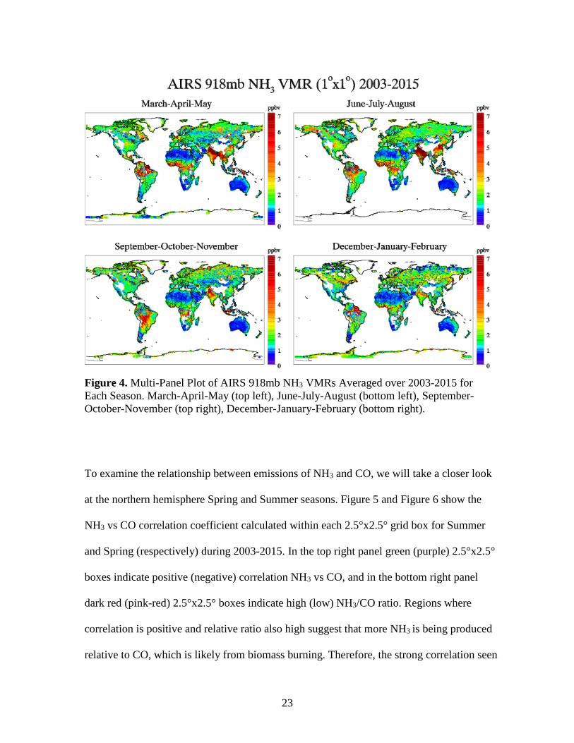
Figure 3 and Figure 4 show the global distribution maps for AIRS CO VMR and AIRS

NH3 VMR, respectively, for the four seasons over the 13-year period. As seen from Figure

3, CO VMR is lower in northern hemisphere Summer and Fall due to increase

photochemical processes resulting from increased plant growth while it is much higher in

the Winter and Spring months due to lack of plant growth and therefore CO accumulates.

In Figure 4, the differences in NH3 VMR between the four seasons can mostly be attributed

to changes biomass burning and fertilizer applications and animal feeding from season to

season.

22

Figure 3. Multi-Panel Plot of AIRS 505mb CO VMRs Averaged over 2003-2015 for Each Season. March-April-May (top left), June-July-August (bottom left), September-October-November (top right), December-January-February (bottom right).

23

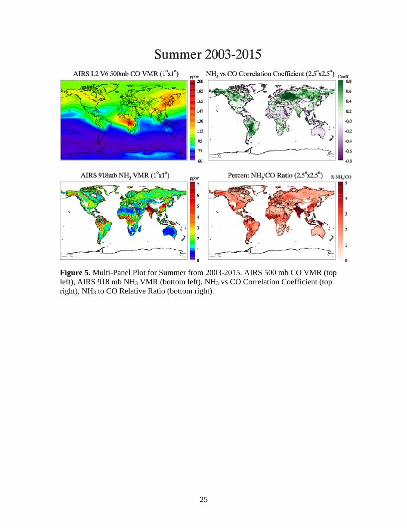
Figure 4. Multi-Panel Plot of AIRS 918mb NH3 VMRs Averaged over 2003-2015 for Each Season. March-April-May (top left), June-July-August (bottom left), September-October-November (top right), December-January-February (bottom right). To examine the relationship between emissions of NH3 and CO, we will take a closer look

at the northern hemisphere Spring and Summer seasons. Figure 5 and Figure 6 show the

NH3 vs CO correlation coefficient calculated within each 2.5°x2.5° grid box for Summer

and Spring (respectively) during 2003-2015. In the top right panel green (purple) 2.5°x2.5°

boxes indicate positive (negative) correlation NH3 vs CO, and in the bottom right panel

dark red (pink-red) 2.5°x2.5° boxes indicate high (low) NH3/CO ratio. Regions where

correlation is positive and relative ratio also high suggest that more NH3 is being produced

relative to CO, which is likely from biomass burning. Therefore, the strong correlation seen

24

in Figure 5 over Alaska and Russia during NH Summer can be categorized as biomass

burning regions, which are most likely due to sporadic wildfire events. Furthermore, the

high NH3/CO ratio also within these regions may hint that the vegetation and/or soil at

higher latitudes release more NH3 relative to CO than in tropical regions. During NH

Spring background CO concentrations have built up over the winter due to increased

lifetime (decreased sinks), resulting in large emission and source differences compared to

NH3. Such cases can be seen from Figure 6; where correlation is negative, indicated by

purple squares, and the relative emission NH3 is higher than CO which generally indicates

a non-biomass burning region (agriculture or industrial sites).

Regions such as North-Central China and South-Central Asia where NH3 and CO are very

strongly correlated for the majority of the year, but are also characterized as highly

populated, industrialized, and also have seasonal agriculture practices are difficult to

understand since they have mixed sources. These type of regions (and/or seasons) present

conflicting positive/negative correlation and high/low relative VMR ratio cases, and thus

cannot be designated as either a biomass burning or anthropogenic dominated

region/season. As a result of these uncategorized “mixed source” cases it not reasonable to

identify global fire regions solely by high NH3 vs CO correlations. Therefore, a “threshold”

value may be determined to help locate/pinpoint a separation between; biomass burning

dominating high NH3 and CO regions, from anthropogenic dominating high NH3 regions.

This concept will be further discussed in the next “Section 3.2 Identifying Fire Regions

Using a ‘Threshold’”, where a preliminary “threshold” value will be proposed to locate fire

regions in addition to strong correlation.

25

Figure 5. Multi-Panel Plot for Summer from 2003-2015. AIRS 500 mb CO VMR (top left), AIRS 918 mb NH3 VMR (bottom left), NH3 vs CO Correlation Coefficient (top right), NH3 to CO Relative Ratio (bottom right).

26

Figure 6. Multi-Panel Plot for Spring from 2003-2015. AIRS 500 mb CO VMR (top left), AIRS 918 mb NH3 VMR (bottom left), NH3 vs CO Correlation Coefficient (top right), NH3 to CO Relative Ratio (bottom right).

3.2 Identifying Fire Regions Using a “Threshold”

During this Section, a MODIS Global Monthly Fire Location Product will be used to assist

and advance the understanding of the emission differences between NH3 and CO outlined

in the previous Section. The addition of MODIS Average FRP and Total Fire Count data

will support the current analysis through validation in choosing a “threshold” value. The

“threshold” selected is intended to be used coupled with NH3 vs CO correlation coefficients

to better identify and constrain critical fire regions. After testing multiple options the

“threshold” of where NH3 vs CO correlation coefficient > 0.6 was selected.

27

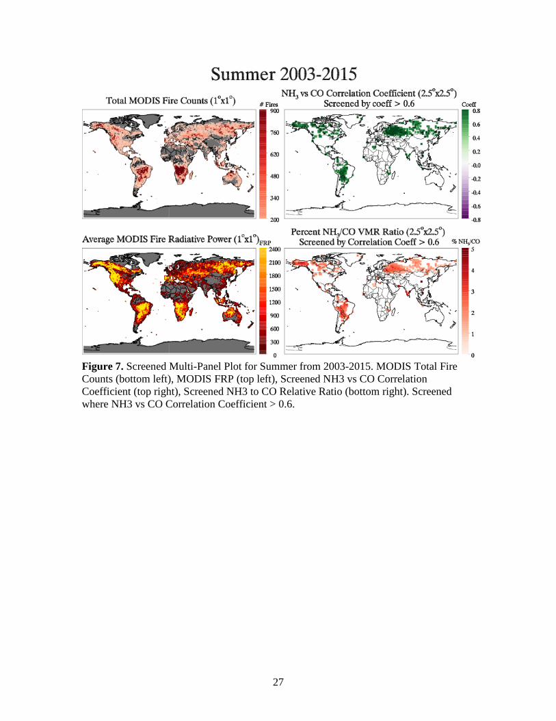
Figure 7. Screened Multi-Panel Plot for Summer from 2003-2015. MODIS Total Fire Counts (bottom left), MODIS FRP (top left), Screened NH3 vs CO Correlation Coefficient (top right), Screened NH3 to CO Relative Ratio (bottom right). Screened where NH3 vs CO Correlation Coefficient > 0.6.

28

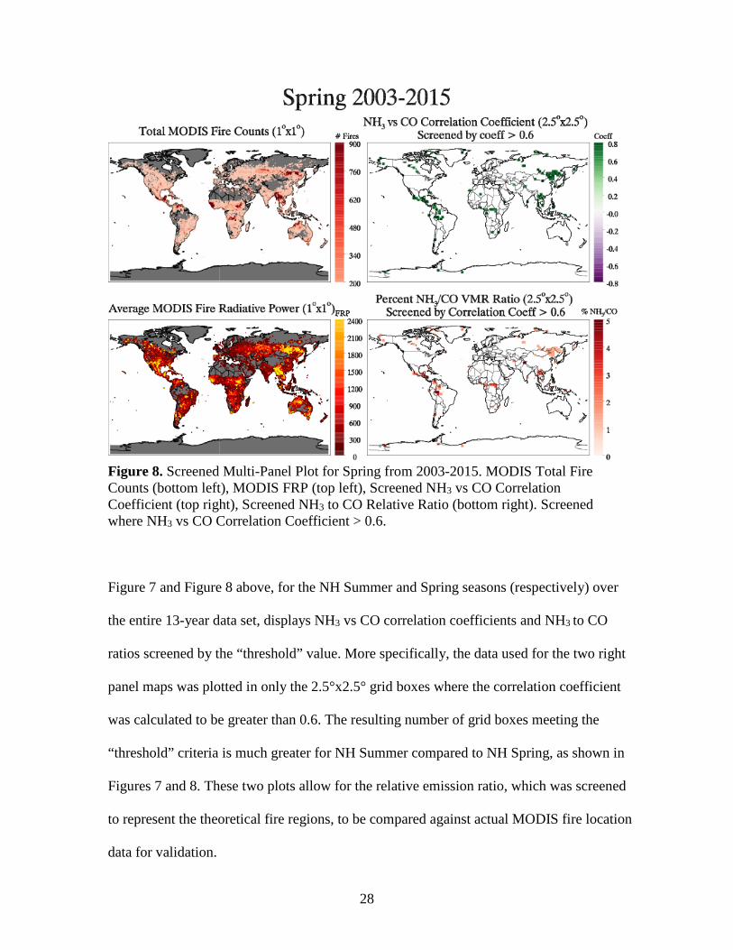
Figure 8. Screened Multi-Panel Plot for Spring from 2003-2015. MODIS Total Fire Counts (bottom left), MODIS FRP (top left), Screened NH3 vs CO Correlation Coefficient (top right), Screened NH3 to CO Relative Ratio (bottom right). Screened where NH3 vs CO Correlation Coefficient > 0.6.

Figure 7 and Figure 8 above, for the NH Summer and Spring seasons (respectively) over

the entire 13-year data set, displays NH3 vs CO correlation coefficients and NH3 to CO

ratios screened by the “threshold” value. More specifically, the data used for the two right

panel maps was plotted in only the 2.5°x2.5° grid boxes where the correlation coefficient

was calculated to be greater than 0.6. The resulting number of grid boxes meeting the

“threshold” criteria is much greater for NH Summer compared to NH Spring, as shown in

Figures 7 and 8. These two plots allow for the relative emission ratio, which was screened

to represent the theoretical fire regions, to be compared against actual MODIS fire location

data for validation.

29

For NH Summer the highest values for MODIS Total Fire Counts and average FRP,

indicated by dark red and bright yellow respectively, match well to the screened data

locations on the right panel. In addition to being reoccurring seasonal wild fire regions, the

stand out hot spots over Russia, Alaska and South America are the result of very large fires

that occurred over the years 2009-2011, specifically in these regions, producing high NH3

concentrations for weeks (R’Honi et al., 2013). As an initial assessment, this indicate that

0.6 is relatively successful (except for a few areas such as Southern Africa) at selecting

important fire region. It is important to note that in some instances areas that are showing

“no data” for NH3 and CO, particularly Southern Africa for example, may be due to

retrieval difficulties and therefore lacking representation in those areas. Despite the smaller

number of grids containing correlation coefficient greater than 0.6, the NH Spring hot spots

designated by MODIS fire data still match relatively well to the screened correlation

coefficient and ratio data. For example, the thin line of screened grid boxes in Africa just

south of the equator represents the shift in seasonal fire locations between NH Spring and

Summer as it starts in the northern part of southern Africa during NH Spring, and then

begins moving south as the season changes to NH Summer. Additionally, the signal shown

for South East Asia is representative of the many fires burning each year as the dry season

ends and people are clearing their fields.

3.3 Regional Time Series of NH3, CO, and MODIS Total Fire Counts

In this Section, the relative emissions of NH3 to CO are examined for various fire regions

over the entire 13 year data set. This is done by creating a time series plot containing a

30

monthly average of NH3 and CO VMR and the Total Monthly MODIS Fire Counts for fire

regions of interest. The first four fire regions were selected based off Giglio et al., (2010)

and a recent study conducted by Whitburn et al., (2014). The regions “Alaska/CA” and

“Russia” were also added. The six regions shown in Figure 9 are; Africa North of the

Equator, Africa South of the Equator, Central South America, and South East Asia. The

minimum and maximum latitude and longitude values used for each region can be found in

Table 1.

Figure 9 Map indicating the location of the 6 fire regions to be investigated.

Region Latitude Min/Max Longitude Min/Max Africa North of Equator 0° to 10°N 15° W to 40° E Africa South of Equator 20° S to 5°S 10° E to 40° E Central South America 20° S to 0°S 65° W to 35° W South East Asia 10° N to 25°N 90° E to 110° E Alaska/CA 60° N to 70° N 165° W to 120° W Russia 50° N to 60° N 15° E to 45° E

Table 1. The minimum and maximum bounding latitude and longitude values for the 6 chosen fire regions of interest.

31

Figure 10a. Regional Trends of AIRS NH3 and CO VMR (ppbv) with Total MODIS Fire Counts for Africa North of the Equator, Africa South of the Equator, Central South America, and South East Asia from 2003-2015. The x-axis is labeled every 3 months (January, April, July, October).

32

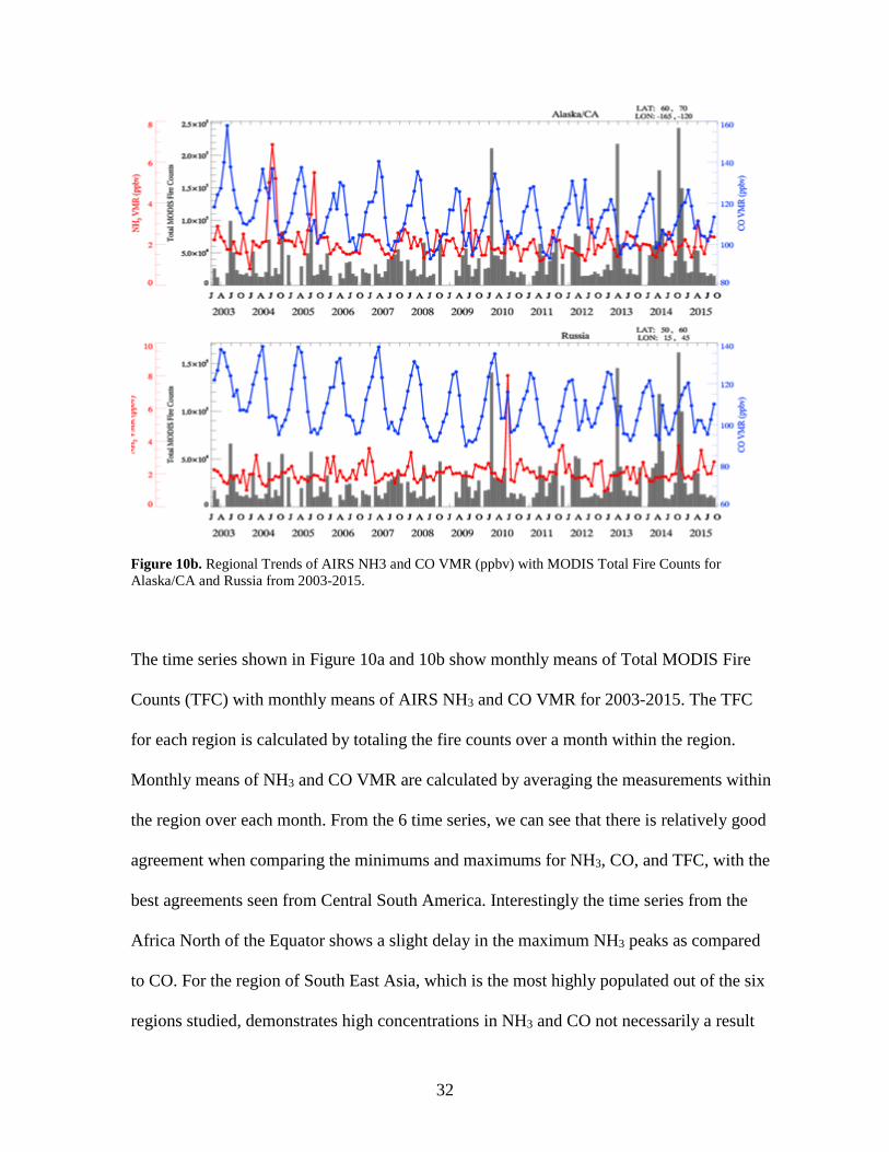
Figure 10b. Regional Trends of AIRS NH3 and CO VMR (ppbv) with MODIS Total Fire Counts for Alaska/CA and Russia from 2003-2015.

The time series shown in Figure 10a and 10b show monthly means of Total MODIS Fire

Counts (TFC) with monthly means of AIRS NH3 and CO VMR for 2003-2015. The TFC

for each region is calculated by totaling the fire counts over a month within the region.

Monthly means of NH3 and CO VMR are calculated by averaging the measurements within

the region over each month. From the 6 time series, we can see that there is relatively good

agreement when comparing the minimums and maximums for NH3, CO, and TFC, with the

best agreements seen from Central South America. Interestingly the time series from the

Africa North of the Equator shows a slight delay in the maximum NH3 peaks as compared

to CO. For the region of South East Asia, which is the most highly populated out of the six

regions studied, demonstrates high concentrations in NH3 and CO not necessarily a result

33

of biomass burning. The primary sources in this region may primarily be anthropogenic

such as livestock and other agricultural practices. From all 6 time series, the increased fire

activity of 2010 can be seen from the amplified NH3 and CO peaks.

Chapter 3. Conclusions & Summary

The primary purpose of this study was to investigate the relationship between NH3 and CO

emissions from fires in different regions, over various vegetation/land types, and how these

differences change over seasonal and decadal time scales using 13 years of satellite

measurements from AIRS. By looking at the global distribution of NH3 and CO VMR from

2003-2015 we showed that there is a seasonal cycle in both the Northern and Southern

Hemisphere. In the Northern Hemisphere the NH3 and CO peaks are more pronounced due

to industrialization, higher populations, and therefore more agriculture practices. In the

Southern Hemisphere the peaks are less pronounces and largely determined by biomass

burning activity.

Seasonal correlations of NH3 vs CO and NH3 to CO relative emission ratios show that, for

most cases, positive correlation indicates regions of biomass burning while negative

correlation indicates regions of agricultural practices. After determining a “threshold” of

correlation coefficient > 0.6, comparisons of the screened correlation and emission ratios to

MODIS Total Fire Counts and Fire Radiative Power confirm the “thresholds” ability to

help separate true fire regions. Further examination of the time series of NH3 and CO VMR

with MODIS Fire Counts of 6 selected fire regions demonstrated the expected agreement

between peaks in concentrations and fires.

34

To more completely understand the relationship between NH3 and CO emissions from fires

an in-depth study incorporating emission factors from different vegetation and land types is

necessary. Although this study has provided significant insight to biomass burning “hot

spot” identification there is still much to be considered, particularly for cases where it is

difficult to differentiate the sources of NH3 and CO emissions.

35

References

Abbatt, J. P. D., Benz, S., Cziczo, D. J., Kanji, Z., Lohmann, U. and Mohler, O.: Solid Ammonium Sulfate Aerosols as Ice Nuclei: A Pathway for Cirrus Cloud Formation, Science (80-. )., 313(September), 1770–1773, 2006.

Adams, P. J., Seinfeld, J. H., Koch, D., Mickley, L. and Jacob, D.: General circulation model assessment of direct radiative forcing by the sulfate-nitrate-ammonium-water inorganic aerosol system, J. Geophys. Res. Atmos., 106(1), 1097–1111, doi:10.1029/2000JD900512, 2001.

Akagi, S. K., Yokelson, R. J., Wiedinmyer, C., Alvarado, M. J., Reid, J. S., Karl, T., Crounse, J. D. and Wennberg, P. O.: Emission factors for open and domestic biomass burning for use in atmospheric models, Atmos. Chem. Phys., 11(9), 4039–4072, doi:10.5194/acp-11-4039-2011, 2011.

Aneja, V. P., Roelle, P. A., Murray, G. C., Southerland, J., Erisman, J. W., Fowler, D., Asman, W. A. H. and Patni, N.: Atmospheric nitrogen compounds. II: Emissions, transport, transformation, deposition and assessment, Atmos. Environ., 35(11), 1903–1911, doi:10.1016/S1352-2310(00)00543-4, 2001.

Aneja, V. P., Schlesinger, W. H. and Erisman, J. W.: Farming pollution, Nat. Geosci., 1(7), 409–411, doi:10.1038/ngeo236, 2008.

Aumann, H. H., Chahine, M. T., Gautier, C., Goldberg, M. D., Kalnay, E., McMillin, L. M., Revercomb, H., Rosenkranz, P. W., Smith, W. L., Staelin, D. H., Strow, L. L. and Susskind, J.: AIRS/AMSU/HSB on the aqua mission: Design, science objectives, data products, and processing systems, IEEE Trans. Geosci. Remote Sens., 41(2 PART 1), 253–263, doi:10.1109/TGRS.2002.808356, 2003.

Aumann, H. H. H. and Miller, C. R. C.: Atmospheric infrared sounder (AIRS) on the Earth Observing System, Proc. SPIE, 2583(December 15, 1995), 332–343, doi:10.1117/12.228579, 1995.

Badr, O. and Probert, S. D.: Carbon monoxide concentration in the Earth’s atmosphere, Appl. Energy, 49(2), 99–143, doi:10.1016/0306-2619(94)90035-3, 1994.

Beer, R., Shephard, M. W., Kulawik, S. S., Clough, S. A., Eldering, A., Bowman, K. W., Sander, S. P., Fisher, B. M., Payne, V. H., Luo, M., Osterman, G. B. and Worden, J. R.: First satellite observations of lower tropospheric ammonia and methanol, Geophys. Res. Lett., 35(9), 1–5, doi:10.1029/2008GL033642, 2008.

Behera, S. N. and Sharma, M.: Investigating the potential role of ammonia in ion chemistry of fine particulate matter formation for an urban environment, Sci. Total Environ., 408(17), 3569–3575, doi:10.1016/j.scitotenv.2010.04.017, 2010.

36

Behera, S. N. and Sharma, M.: Transformation of atmospheric ammonia and acid gases into components of PM2.5: An environmental chamber study, Environ. Sci. Pollut. Res., 19(4), 1187–1197, doi:10.1007/s11356-011-0635-9, 2012.

Bey, I., Jacob, D. J., Yantosca, R. M., Logan, J. A., Field, B. D., Fiore, A. M., Li, Q.-B., Liu, H.-Y., Mickley, L. J. and Schultz, M. G.: Global Modeling of Tropospheric Chemistry with Assimilated Meteorology: Model Description and Evaluation, J. Geophys. Res., 106, 73–95, doi:10.1029/2001JD000807, 2001.

Brook, R. D., Rajagopalan, S., Pope, C. A., Brook, J. R., Bhatnagar, A., Diez-Roux, A. V., Holguin, F., Hong, Y., Luepker, R. V., Mittleman, M. A., Peters, A., Siscovick, D., Smith, S. C., Whitsel, L. and Kaufman, J. D.: Particulate matter air pollution and cardiovascular disease: An update to the scientific statement from the american heart association, Circulation, 121(21), 2331–2378, doi:10.1161/CIR.0b013e3181dbece1, 2010.

Clarisse, L., Clerbaux, C., Dentener, F., Hurtmans, D. and Coheur, P.-F.: Global ammonia distribution derived from infrared satellite observations, Nat. Geosci., 2(7), 479–483, doi:10.1038/ngeo551, 2009.

Clarisse, L., Shephard, M. W., Dentener, F., Hurtmans, D., Cady-Pereira, K., Karagulian, F., Van Damme, M., Clerbaux, C. and Coheur, P. F.: Satellite monitoring of ammonia: A case study of the San Joaquin Valley, J. Geophys. Res., 115, doi:10.1029/2009jd013291, 2010.

Coheur, P.-F., Clarisse, L., Turquety, S., Hurtmans, D. and Clerbaux, C.: IASI measurements of reactive trace species in biomass burning plumes, Atmos. Chem. Phys. Discuss., 9(2), 8757–8789, doi:10.5194/acpd-9-8757-2009, 2009.

Crutzen, P. J., Heidt, L. E., Krasnec, J. P., Pollock, W. H. and Seiler, W.: Biomass burning as a source of atmospheric gases CO, H2, N2O, NO, CH3Cl and COS, Nature, 282(5736), 253–256, doi:10.1038/282253a0, 1979.

Van Damme, M., Clarisse, L., Heald, C. L., Hurtmans, D., Ngadi, Y., Clerbaux, C., Dolman, A. J., Erisman, J. W. and Coheur, P. F.: Global distributions, time series and error characterization of atmospheric ammonia (NH3) from IASI satellite observations, Atmos. Chem. Phys., 14(6), 2905–2922, doi:10.5194/acp-14-2905-2014, 2014.

Van Damme, M., Clarisse, L., Dammers, E., Liu, X., Nowak, J. B., Clerbaux, C., Flechard, C. R., Galy-Lacaux, C., Xu, W., Neuman, J. A., Tang, Y. S., Sutton, M. A., Erisman, J. W. and Coheur, P. F.: Towards validation of ammonia (NH3) measurements from the IASI satellite, Atmos. Meas. Tech., 8(3), 1575–1591, doi:10.5194/amt-8-1575-2015, 2015.

Demarest, P., Richon, K. V. and Wright, F.: Analysis for Monitoring the Earth Science Afternoon Constellation, in AAS/AIAA Astrodynamic Specialist Conference, p. AAS 05-368., 2005.

37

Fowler, D., Coyle, M., Skiba, U., Sutton, M. A., Cape, J. N., Reis, S., Sheppard, L. J., Jenkins, A., Grizzetti, B., Galloway, N., Vitousek, P., Leach, A., Bouwman, A. F., Butterbach-bahl, K., Dentener, F., Stevenson, D., Amann, M., Voss, M. and Fowler, D.: The global nitrogen cycle in the twenty- first century, Phil. Trans. R. Soc. B, 368(2621), 2013.

Galloway, J. N., Townsend, A. R., Erisman, J. W., Bekunda, M., Cai, Z., Freney, J. R., Martinelli, L. A., Seitzinger, S. P. and Sutton, M. A.: Transformation of the Nitrogen Cycle: Recent trends, questions, and potential solutions, Science (80-. )., 320, 889–893, 2008.

Giglio, L.: MODIS Collection 6 Active Fire Product User’s Guide Revision A. [online] Available from: http://modis-fire.umd.edu/files/MODIS_C6_Fire_User_Guide_A.pdf, 2015.

Giglio, L., van der Werf, G. R., Randerson, J. T., Collatz, G. J. and Kasibhatla, P.: Global estimation of burned area using MODIS active fire observations, Atmos. Chem. Phys. Discuss., 5(6), 11091–11141, doi:10.5194/acpd-5-11091-2005, 2006.

Giglio, L., Randerson, J. T., Van Der Werf, G. R., Kasibhatla, P. S., Collatz, G. J., Morton, D. C. and Defries, R. S.: Assessing variability and long-term trends in burned area by merging multiple satellite fire products, Biogeosciences, 7(2008), 1171–1186, doi:10.5194/bg-7-1171-2010, 2010.

Giglio, L., Schroeder, W. and Justice, C. O.: The collection 6 MODIS active fire detection algorithm and fire products, Remote Sens. Environ., 178, 31–41, doi:10.1016/j.rse.2016.02.054, 2016.

Heald, C. L., Collett, J. L., Lee, T., Benedict, K. B., Schwandner, F. M., Li, Y., Clarisse, L., Hurtmans, D. R., Van Damme, M., Clerbaux, C., Coheur, P. F., Philip, S., Martin, R. V. and Pye, H. O. T.: Atmospheric ammonia and particulate inorganic nitrogen over the United States, Atmos. Chem. Phys., 12(21), 10295–10312, doi:10.5194/acp-12-10295-2012, 2012.

IPCC: Anthropogenic and Natural Radiative Forcing., 2013.

Justice, C. O., Giglio, L., Korontzi, S., Owens, J., Morisette, J. T., Roy, D., Descloitres, J., Alleaume, S., Petitcolin, F. and Kaufman, Y.: The MODIS fire products, Remote Sens. Environ., 83(1–2), 244–262, doi:10.1016/S0034-4257(02)00076-7, 2002.

Langridge, J. M., Lack, D., Brock, C. A., Bahreini, R., Middlebrook, A. M., Neuman, J. A., Nowak, J. B., Perring, A. E., Schwarz, J. P., Spackman, J. R., Holloway, J. S., Pollack, I. B., Ryerson, T. B., Roberts, J. M., Warneke, C., De Gouw, J. A., Trainer, M. K. and Murphy, D. M.: Evolution of aerosol properties impacting visibility and direct climate forcing in an ammonia-rich urban environment, J. Geophys. Res. Atmos., 117(6), 1–17, doi:10.1029/2011JD017116, 2012.

Luo, M., Shephard, M. W., Cady-Pereira, K. E., Henze, D. K., Zhu, L., Bash, J. O.,

38

Pinder, R. W., Capps, S. L., Walker, J. T. and Jones, M. R.: Satellite observations of tropospheric ammonia and carbon monoxide: Global distributions, regional correlations and comparisons to model simulations, Atmos. Environ., 106, 262–277, doi:10.1016/j.atmosenv.2015.02.007, 2015.

NASA: EOS Science Plan: The State of Science in the EOS Program., 1999.

Pinder, R. W., Adams, P. J., Pandis, S. N. and Gilliland, A. B.: Temporally resolved ammonia emission inventories: Current estimates, evaluation tools, and measurement needs, J. Geophys. Res. Atmos., 111(16), 1–14, doi:10.1029/2005JD006603, 2006.

Pope, C. A. and Dockery, D. W.: Health Effects of Fine Particulate Air Pollution: Lines that Connect, J. Air Waste Manage. Assoc., 56(6), 709–742, 2006.

Pope, C. A., Brook, R. D., Burnett, R. T. and Dockery, D. W.: How is cardiovascular disease mortality risk affected by duration and intensity of fine particulate matter exposure? An integration of the epidemiologic evidence, Air Qual. Atmos. Heal., 4(1), 5–14, doi:10.1007/s11869-010-0082-7, 2011.

R’Honi, Y., Clarisse, L., Clerbaux, C., Hurtmans, D., Duflot, V., Turquety, S., Ngadi, Y. and Coheur, P. F.: Exceptional emissions of NH3 and HCOOH in the 2010 Russian wildfires, Atmos. Chem. Phys., 13(1), 4171–4181, doi:10.5194/acp-13-4171-2013, 2013.

Schoeberl, M. R., Douglass, A. R., Hilsenrath, E., Bhartia, P. K., Barnett, J., Gille, J., Beer, R., Gunson, M., Walters, J., Levelt, P. F. and DeCola, P.: Earth Observing System Missions Benefit Atmospheric Research, EOS Trans. AGU, 85(18), 177–181, 2004.

Shephard, M. W. and Cady-Pereira, K. E.: Cross-track Infrared Sounder (CrIS) satellite observations of tropospheric ammonia, Atmos. Meas. Tech., 8(3), 1323–1336, doi:10.5194/amt-8-1323-2015, 2015.

Shephard, M. W., Cady-Pereira, K. E., Luo, M., Henze, D. K., Pinder, R. W., Walker, J. T., Rinsland, C. P., Bash, J. O., Zhu, L., Payne, V. H. and Clarisse, L.: TES ammonia retrieval strategy and global observations of the spatial and seasonal variability of ammonia, Atmos. Chem. Phys., 11(20), 10743–10763, doi:10.5194/acp-11-10743-2011, 2011.

Shukla, S. P. and Sharma, M.: Neutralization of rainwater acidity at Kanpur, India, Tellus, Ser. B Chem. Phys. Meteorol., 62(3), 172–180, doi:10.1111/j.1600-0889.2010.00454.x, 2010.

Susskind, J., Barnet, C. D. and Blaisdell, J. M.: Retrieval of Atmospheric and Surface Parameters From AIRS / AMSU / HSB Data in the Presence of Clouds, IEEE Trans. Geosci. Remote Sens., 41(2), 390–409, doi:10.1109/TGRS.2002.808236, 2003.

Sutton, M. A., Erisman, J. W., Dentener, F. and Möller, D.: Ammonia in the environment: From ancient times to the present, Environ. Pollut., 156(3), 583–604, doi:10.1016/j.envpol.2008.03.013, 2008.

39

Updyke, K. M., Nguyen, T. B. and Nizkorodov, S. A.: Formation of brown carbon via reactions of ammonia with secondary organic aerosols from biogenic and anthropogenic precursors, Atmos. Environ., 63, 22–31, doi:10.1016/j.atmosenv.2012.09.012, 2012.

Walker, J. M., Philip, S., Martin, R. V. and Seinfeld, J. H.: Simulation of nitrate, sulfate, and ammonium aerosols over the United States, Atmos. Chem. Phys., 12(22), 11213–11227, doi:10.5194/acp-12-11213-2012, 2011.

Warner, J., Carminati, F., Wei, Z., Lahoz, W. and Attié, J. L.: Tropospheric carbon monoxide variability from AIRS under clear and cloudy conditions, Atmos. Chem. Phys., 13(24), 12469–12479, doi:10.5194/acp-13-12469-2013, 2013.

Warner, J. X., Wei, Z., Strow, L. L., Barnet, C. D., Sparling, L. C., Diskin, G. and Sachse, G.: Improved agreement of AIRS tropospheric carbon monoxide products with other EOS sensors using optimal estimation retrievals, Atmos. Chem. Phys., 10(19), 9521–9533, doi:10.5194/acp-10-9521-2010, 2010.

Warner, J. X., Wei, Z., Larrabee Strow, L., Dickerson, R. R. and Nowak, J. B.: The global tropospheric ammonia distribution as seen in the 13-year AIRS measurement record, Atmos. Chem. Phys., 16(8), 5467–5479, doi:10.5194/acp-16-5467-2016, 2016.

van der Werf, G. R., Randerson, J. T., Giglio, L., Collatz, G. J., Kasibhatla, P. S. and Arellano, A. F., J.: Interannual variability in global biomass burning emissions from 1997 to 2004, Atmos. Chem. Phys., 6(11), 3423–3441, doi:10.5194/acpd-6-3175-2006, 2006.

Whitburn, S., Van Damme, M., Kaiser, J. W., Van Der Werf, G. R., Turquety, S., Hurtmans, D., Clarisse, L., Clerbaux, C. and Coheur, P. F.: Ammonia emissions in tropical biomass burning regions: Comparison between satellite-derived emissions and bottom-up fire inventories, Atmos. Environ., 121, 42–54, doi:10.1016/j.atmosenv.2015.03.015, 2014.

Wooster, M. J., Roberts, G., Perry, G. L. W. and Kaufman, Y. J.: Retrieval of biomass combustion rates and totals from fire radiative power observations: FRP derivation and calibration relationships between biomass consumption and fire radiative energy release, J. Geophys. Res. Atmos., 110(24), 1–24, doi:10.1029/2005JD006318, 2005.