Identifying and Evaluating Contrarian Strategiesfor NCAA Tournament Pools

Submitted in Partial Fulfillment of the Requirements forMaster of Science Degree

In BiostatisticsDivision of BiostatisticsSchool of Public HealthUniversity of Minnesota

Minneapolis, MN

ByJarad B. Niemi

June 7, 2005

Committee MembersBradley Carlin, PhD Chair

John Connett, PhDGalin Jones, PhD

Identifying and Evaluating Contrarian Strategiesfor NCAA Tournament Pools

Abstract

The annual NCAA men’s basketball tournament inspires many individuals to wager money in office and

online pools that require entrants to predict the outcome of every game prior to the tournament’s onset.

Coupled with the haphazard team selection behavior of many casual players, office pools’ complexity suggests

the possible existence of well-informed strategies that are profitable in the long run. Previous work in this area

has focused on development of strategies that attempt to maximize the expected score of a set of selections.

Unfortunately, the vast majority of pools use simple scoring schemes that do not reward the correct picking of

upsets, meaning that an entry sheet that maximizes expected points will feature mostly favorites. This in turn

means the sheet will have too much in common with many other players’ sheets to be profitable. In this article,

we seek to identify strategies that are contrarian in the sense that they favor teams that have a high probability

of winning, yet are likely to be underbet by our opponents relative to other teams in the pool. Using 2003-2005

data from a medium-sized ongoing Chicago-based office pool, we show that such strategies can outperform

the maximum expected score strategy in terms of expected payoff. We also developed “predicted contrarian”

approaches that tackle the more difficult case where we assume opponent betting behavior is unknown, but

may be estimated using web-downloadable data on the teams in the tournament.

Key words: Basketball; March madness; Office pool; Point spread; Team ratings.

1 Introduction

Every March the National Collegiate Athletic Association (NCAA) selects 65 Division I teams to compete

in a single-elimination tournament to determine a single college basketball national champion. Due to the

frequency of upsets that occur every year, this event has been dubbed “March Madness” by the media who

cover the much-hyped and much-wagered upon event. The tournament tempts individuals to wager money

in online or office pools in which the goal is to predict, prior to its onset, the outcome of every game. A

prespecified scoring scheme, typically assigning more points to correct picks in later tournament rounds, is

used to score each entry sheet. As in horse racing, the betting is parimutuel: the players with the highest-

1

scoring sheets win predetermined shares of the total money wagered. In most states, such pools are considered

legal provided the poolmaster does not accept remuneration of any kind, including his own entry fee.

Many strategies exist for choosing one’s sheet, such as picking by team rankings, winning percentages,

expert advice, color of uniforms, etc. Previous articles such as Breiter and Carlin (1997) and Kaplan and

Garstka (2001) have described methods to maximize expected total score. These methods can have high

expected return on investment (ROI) when the scoring scheme is complex, particularly when it awards a

large proportion of the total points for correctly predicting upsets. Tom Adams’s website, www.poologic.com,

provides a Java-based implementation of the method of Breiter and Carlin (1997) using the fast algorithm

of Kaplan and Garstka (2001) for a wide variety of pool scoring systems. This website can also produce the

highest expected point total sheet subject to the constraint that the champion is a particular team.

Most office pool scoring schemes are relatively simple and do not reward the picking of upsets. In such

cases, the sheet that maximizes expected points often does not deliver high expected ROI, since it will typically

predict few upsets, and thus have too much in common with other bettors’ sheets to be profitable in a

parimutuel system. Metrick (1996) observed that pool participants tend to overback heavily favored teams,

and shows how a bettor can use this to advantage in a simplified, “pick the tournament champion only”

pool. Clair and Letscher (2005) describe an approach for maximizing expected ROI in weekly football and

NCAA basketball pools if opponent betting behavior is known. Strategies like these that account for team

win probabilities while simultaneously seeking to avoid the most popular team choices are sometimes referred

to as contrarian.

In this paper, we discuss a method to increase expected ROI without precise knowledge of opponents’ bets.

This method involves a contrarian strategy whose objective is to identify teams that have a high probability

of winning, but are likely to be “underbet” relative to other teams in the pool. Section 2 discusses probability

models that are necessary in developing a pool betting strategy. Section 3 then presents the specific office pool

data we consider, as well as a set of team-specific covariates that may be useful in predicting opponent betting

behavior. Section 4 introduces some statistical terminology and formulae needed in our analysis. Following a

motivation of the need for contrarian thinking, Section 5 identifies and evaluates contrarian strategies using

our actual pool sheet data. Section 6 discusses how to predict opponent betting and investigates the impact

of imperfect opponent behavior knowledge on our strategies’ ROI. Finally, Section 7 summarizes and offers

suggestions for future work in this area.

2

2 Probability Models for NCAA Basketball Tournaments

To develop an optimal betting strategy whether to maximize expected score or maximize expected ROI,

knowledge of the true game win probabilities is required. In a 64-team tournament, this is equivalent to a

64× 64 matrix A containing entries aij , the actual probability that team i beats team j. The only restrictions

on this matrix are that 0 ≤ aij ≤ 1 and aij = 1 − aji, since no game can end in a tie. In this matrix the aii

are irrelevant since a team will never play itself. Estimation of the resulting 2,016 unknowns is not feasible, so

another assumption must be made. The usual assumption is that each team has a rating, and the probability

that any team beats any other team is a function of the difference in their ratings. By using this assumption,

we restrict ourselves to a no-interaction model, where e.g., aij > aik =⇒ ajk < 12 .

Prior to discussing rating systems, a distinction needs to be made between ranking and rating. Rank-

ings give only the ordering of teams, whereas ratings give the teams’ relative strengths. Thus ratings are

more informative, since one can easily obtain rankings from ratings, but not vice versa. Examples of rank-

ings are the Associated Press and USAToday/ESPN Coaches’ polls, although efforts have been made to turn

these into ratings. Examples of ratings are the Ratings Power Index (RPI) used by the tournament selec-

tion committee, as well as ratings produced by Kenneth Massey (www.masseyratings.com), Jeff Sagarin

(www.usatoday.com/sports/sagarin.htm), and many others.

Schwertman et al. (1991) and Schwertman et al. (1996) discuss ratings based on tournament seed, a number

from 1 to 16 describing a team’s potential opponents at every future stage; stronger teams are assigned to

lower (better) seeds. These ratings suffer because they force a seed to have equal relative strength to that

same seed in another region, or even another tournament.

More sophisticated methods use data from the just-completed season, including team record, opponents’

records, strength of conference, etc. Massey calculates his rating using score, venue, and date, with a Bayesian

correction that helps account for what he calls “correlating performances” (a team playing up or down to its

opponent). Sagarin ratings begin with a Bayesian combination of a set of initial estimates and the current

year’s data until all teams are connected, meaning that every team can be mapped to every other team through

its opponents and its opponents’ opponents, etc. At this point the initial estimates are dropped and the ratings

are based purely on the current season’s data. Sagarin actually offers three ratings: Predictor, Elochess, and

a compromise between these two simply called Sagarin. Predictor uses venue and margin of victory, while

3

Elochess uses only venue and win-loss result. Numerous other ratings exist, but we will focus on these due to

their popularity and free web availability.

Ratings can also be obtained from Las Vegas odds, either alone or in conjunction with one of the other

rating systems. If used alone, ratings for each team can be computed from the first round pre-tournament

spreads and total points (over/under). Specifically, if dij is the point spread for team i versus team j and tij

is the over/under, then the implied ratings Zi and Zj for the two teams are

Zi =tij + dij

2and Zj =

tij − dij

2.

These ratings are obviously completely dependent on a single set of first-round betting lines, and therefore

should be used with caution. They are included in this analysis primarily as a counterpoint to Sagarin ratings.

A better method, suggested by Carlin (1996), may be to use point spreads for first round games and one of

the Sagarin ratings for all future games.

For high-scoring team sports, Stern (1991) shows using historical data that aij can be sensibly chosen as

aij = Φ(

β(Zi − Zj)σ

), (1)

where Φ(·) denotes the cumulative distribution function of the standard normal distribution, β is a blowout

inflation factor, Zi is the rating for team i, and σ is an appropriately chosen standard deviation. The blowout

inflation factor was suggested by Carlin (1996) due to empirical evidence that (1) is an underestimate for

teams of widely differing strengths if β = 1; in this analysis we set β = 1.05. The standard deviation is set at

12 for Sagarin ratings and 1.41 for Massey ratings (Sagarin ratings typically range from 70-100 while Massey

ratings range from 4-7).

3 Available Data

The main source of data used in this analysis is three years’ worth of betting sheets and actual tournament

results for an ongoing Chicago-based office pool. A secondary source is a set of team-specific covariates

potentially useful in predicting betting behavior of the participants in the pool.

4

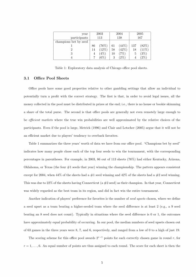
year 2003 2004 2005participants 113 138 167

champions bet by seed1 86 (76%) 61 (44%) 137 (82%)2 14 (12%) 58 (42%) 18 (11%)3 4 (4%) 10 (7%) 5 (3%)4 7 (6%) 3 (2%) 4 (2%)

Table 1: Exploratory data analysis of Chicago office pool sheets.

3.1 Office Pool Sheets

Office pools have some good properties relative to other gambling settings that allow an individual to

potentially turn a profit with the correct strategy. The first is that, in order to avoid legal issues, all the

money collected in the pool must be distributed in prizes at the end; i.e., there is no house or bookie skimming

a share of the total purse. The second is that office pools are generally not even remotely large enough to

be efficient markets where the true win probabilities are well approximated by the relative choices of the

participants. Even if the pool is large, Metrick (1996) and Clair and Letscher (2005) argue that it will not be

an efficient market due to players’ tendency to overback favorites.

Table 1 summarizes the three years’ worth of data we have from our office pool. “Champions bet by seed”

indicates how many people chose each of the top four seeds to win the tournament, with the corresponding

percentages in parentheses. For example, in 2003, 86 out of 113 sheets (76%) had either Kentucky, Arizona,

Oklahoma, or Texas (the four #1 seeds that year) winning the championship. The pattern appears consistent

except for 2004, when 44% of the sheets had a #1 seed winning and 42% of the sheets had a #2 seed winning.

This was due to 22% of the sheets having Connecticut (a #2 seed) as their champion. In that year, Connecticut

was widely regarded as the best team in its region, and did in fact win the entire tournament.

Another indication of players’ preference for favorites is the number of seed upsets chosen, where we define

a seed upset as a team beating a higher-seeded team where the seed difference is at least 2 (e.g., a 9 seed

beating an 8 seed does not count). Typically in situations where the seed difference is 0 or 1, the outcomes

have approximately equal probability of occurring. In our pool, the median numbers of seed upsets chosen out

of 63 games in the three years were 8, 7, and 6, respectively, and ranged from a low of 0 to a high of just 19.

The scoring scheme for this office pool awards 2r−1 points for each correctly chosen game in round r, for

r = 1, . . . , 6. An equal number of points are thus assigned to each round. The score for each sheet is then the

5

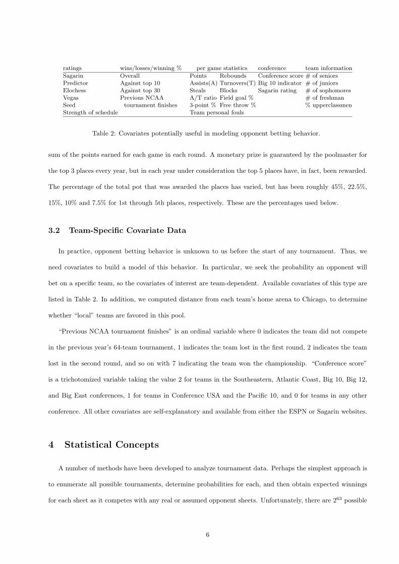
ratings wins/losses/winning % per game statistics conference team information

Sagarin Overall Points Rebounds Conference score # of seniorsPredictor Against top 10 Assists(A) Turnovers(T) Big 10 indicator # of juniorsElochess Against top 30 Steals Blocks Sagarin rating # of sophomoresVegas Previous NCAA A/T ratio Field goal % # of freshmanSeed tournament finishes 3-point % Free throw % % upperclassmenStrength of schedule Team personal fouls

Table 2: Covariates potentially useful in modeling opponent betting behavior.

sum of the points earned for each game in each round. A monetary prize is guaranteed by the poolmaster for

the top 3 places every year, but in each year under consideration the top 5 places have, in fact, been rewarded.

The percentage of the total pot that was awarded the places has varied, but has been roughly 45%, 22.5%,

15%, 10% and 7.5% for 1st through 5th places, respectively. These are the percentages used below.

3.2 Team-Specific Covariate Data

In practice, opponent betting behavior is unknown to us before the start of any tournament. Thus, we

need covariates to build a model of this behavior. In particular, we seek the probability an opponent will

bet on a specific team, so the covariates of interest are team-dependent. Available covariates of this type are

listed in Table 2. In addition, we computed distance from each team’s home arena to Chicago, to determine

whether “local” teams are favored in this pool.

“Previous NCAA tournament finishes” is an ordinal variable where 0 indicates the team did not compete

in the previous year’s 64-team tournament, 1 indicates the team lost in the first round, 2 indicates the team

lost in the second round, and so on with 7 indicating the team won the championship. “Conference score”

is a trichotomized variable taking the value 2 for teams in the Southeastern, Atlantic Coast, Big 10, Big 12,

and Big East conferences, 1 for teams in Conference USA and the Pacific 10, and 0 for teams in any other

conference. All other covariates are self-explanatory and available from either the ESPN or Sagarin websites.

4 Statistical Concepts

A number of methods have been developed to analyze tournament data. Perhaps the simplest approach is

to enumerate all possible tournaments, determine probabilities for each, and then obtain expected winnings

for each sheet as it competes with any real or assumed opponent sheets. Unfortunately, there are 263 possible

6

tournament outcomes, since there are 63 games. Even if we only look at tournaments where the #1 seeds beat

the #16 seeds, the enumeration remains prohibitively large at 259. For this reason, one of the most useful

tools in analyzing tournaments is to simulate a large number of tournaments, using the resulting relative

frequencies of the outcomes to reduce the computation but preserve realism. Other important ideas included

in this section concern ROI, the probability of a sheet, the similarity of a sheet to other sheets in a pool, and

a notion of “underbetness,” the bettors’ perception of a team relative to its actual ability.

4.1 Simulating Return on Investment

To simulate one tournament, we begin with a 64×64 matrix of win probabilities A as described in Section 2.

For each of the 32 first-round matchups, a Uniform(0,1) random number is drawn. If this number is greater

than its aij , team j is the simulated winner, otherwise team i is the winner. This process is then repeated for

each game in each round until a simulated outcome for the entire 63-game tournament is obtained.

For each simulated tournament, all office pool sheets for that year can be scored, ranked, and awarded

prizes as described in Section 3.1. Repeating this process over many simulated tournaments, the ROI for each

sheet may be estimated as

ROI =total won – total invested

total invested.

We standardize this calculation so that each sheet costs $1. An ROI of zero indicates a break-even strategy,

whereas a negative value indicates a losing strategy and a positive value indicates a winning strategy. We will

estimate ROI for each actual sheet for each year and probability model, as well as certain “optimal” sheets

chosen with and without the benefit of knowing the other sheets in the pool. We remark that this distinguishes

our work from that of Clair and Letscher (2005), whose more mathematically sophisticated approach also seeks

optimal contrarian strategies, but assumes perfect pre-tournament knowledge of the aij , the opponents’ sheets,

and a large enough number of opponents that the cost of entering the pool is negligible.

4.2 Probability and Similarity of a Sheet

In an R-round tournament, a pool sheet consists of 2R− 1 picks of game winners, where these winners can

only come from the winners of the previous round. Since there are 2R−r games in each round r, the probability

7

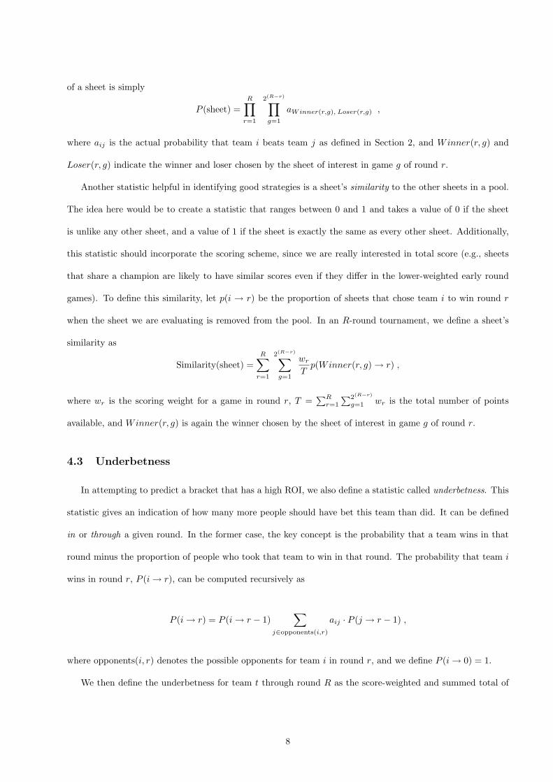
of a sheet is simply

P (sheet) =R∏

r=1

2(R−r)∏g=1

aWinner(r,g), Loser(r,g) ,

where aij is the actual probability that team i beats team j as defined in Section 2, and Winner(r, g) and

Loser(r, g) indicate the winner and loser chosen by the sheet of interest in game g of round r.

Another statistic helpful in identifying good strategies is a sheet’s similarity to the other sheets in a pool.

The idea here would be to create a statistic that ranges between 0 and 1 and takes a value of 0 if the sheet

is unlike any other sheet, and a value of 1 if the sheet is exactly the same as every other sheet. Additionally,

this statistic should incorporate the scoring scheme, since we are really interested in total score (e.g., sheets

that share a champion are likely to have similar scores even if they differ in the lower-weighted early round

games). To define this similarity, let p(i → r) be the proportion of sheets that chose team i to win round r

when the sheet we are evaluating is removed from the pool. In an R-round tournament, we define a sheet’s

similarity as

Similarity(sheet) =R∑

r=1

2(R−r)∑g=1

wr

Tp(Winner(r, g) → r) ,

where wr is the scoring weight for a game in round r, T =∑R

r=1

∑2(R−r)

g=1 wr is the total number of points

available, and Winner(r, g) is again the winner chosen by the sheet of interest in game g of round r.

4.3 Underbetness

In attempting to predict a bracket that has a high ROI, we also define a statistic called underbetness. This

statistic gives an indication of how many more people should have bet this team than did. It can be defined

in or through a given round. In the former case, the key concept is the probability that a team wins in that

round minus the proportion of people who took that team to win in that round. The probability that team i

wins in round r, P (i → r), can be computed recursively as

P (i → r) = P (i → r − 1)∑

j∈opponents(i,r)

aij · P (j → r − 1) ,

where opponents(i, r) denotes the possible opponents for team i in round r, and we define P (i → 0) = 1.

We then define the underbetness for team t through round R as the score-weighted and summed total of

8

seed 1 2 3 4 6 8 totalnumber of wins 12 (57%) 4 (19%) 2 (9.5%) 1 (5%) 1 (5%) 1 (5%) 21 (100%)

Table 3: NCAA basketball championships by seed, 1985–2005.

the individual round values, i.e.,

UR(t) =R∑

r=1

wr[P (t → r)− q · p(t → r)] , (2)

where the wr are the round weights as before. Note this formula also adds a user-defined tuning constant

q ∈ [0, 1] that can be used to trade off the probability and observed proportion; see Subsection 5.5 below.

5 Contrarian Motivation and Strategies

Before developing a contrarian strategy, an important question is whether the idea has demonstrable merit.

In this section, we show that favorites have not done quite as well as predicted by our pool participants, that

most of the sheets in an office pool have low ROI, and that maximizing point total methods also do not have

high ROI. We then turn to the problem of producing contrarian sheets with improved ROI.

5.1 Historical Comparison

It was noted in Subsection 3.1 that the participants in our office pools tend to pick a large percentage of

high seeds (low seed numbers) to win the championship. Since the tournament seeding is set up to put favorites

as higher seeds, this makes sense. Still, it remains to see whether these percentages reflect history. Table 3

gives the number of times a specific seed has won the tournament. In the 21 years of 64-team tournaments, a

#1 seed has won 12 times. So, based on history, we would expect that 57% of the pool sheets would take #1

seeds to win. In reality, Table 1 reveals that #1 seeds were taken to win the championship 76%, 44%, and

82% of the time, an overall 3-year average of 68%. The overall 3-year predicted championship rate of #1 or

#2 seeds is 374/418=89%, compared with the historical rate of 16/21=76%. If the strength of the seeds were

comparable from year to year, we would expect that, if the office pools formed an efficient market, these rates

would be similar. Instead, the percentage of high seeds predicted to win the championship is significantly

larger than the historical average, indicating a possible long-run edge for the contrarian gambler to exploit.

9

2003

−1 0 1 2 3 4 5

0.0

0.1

0.2

0.3

0.4

< 0: 60 %> 1: 7 %

Sagarin20

04

−1 0 1 2 3 4 5

0.0

0.1

0.2

0.3

0.4

< 0: 62 %> 1: 8 %

2005

−1 0 1 2 3 4 5

0.0

0.1

0.2

0.3

0.4

< 0: 64 %> 1: 13 %

−1 0 1 2 3 4 5

0.0

0.1

0.2

0.3

0.4

< 0: 63 %> 1: 12 %

Predictor

−1 0 1 2 3 4 5

0.0

0.1

0.2

0.3

0.4

< 0: 67 %> 1: 11 %

−1 0 1 2 3 4 5

0.0

0.1

0.2

0.3

0.4

< 0: 63 %> 1: 16 %

−1 0 1 2 3 4 5

0.0

0.1

0.2

0.3

0.4

< 0: 62 %> 1: 8 %

Elochess

−1 0 1 2 3 4 5

0.0

0.1

0.2

0.3

0.4

< 0: 65 %> 1: 10 %

−1 0 1 2 3 4 5

0.0

0.1

0.2

0.3

0.4

< 0: 62 %> 1: 12 %

0 5 10 15

0.0

0.2

0.4

0.6

0.8

< 0: 75 %> 1: 7 %

Vegas

0 5 10 15

0.0

0.2

0.4

0.6

0.8

< 0: 67 %> 1: 7 %

0 5 10 15

0.0

0.2

0.4

0.6

0.8

< 0: 82 %> 1: 8 %

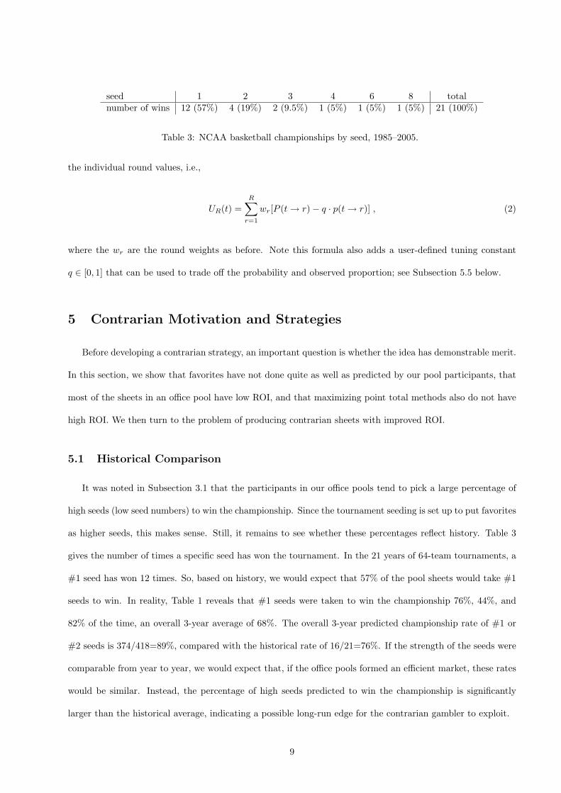
Figure 1: Histograms of simulated ROI for all poolsheets across years and probability models.

5.2 ROI Simulation

The historical evidence for players overbacking favorites motivates a simulation study of how individuals

in our pools would have fared in the long run had the tournaments been played repeatedly. To accomplish

this we need to assume a probability model for true win probabilities aij . We used the four sets of ratings

described in Section 2 to simulate 1,000 tournaments for each year. Histograms of these results can be seen in

Figure 1. The rows correspond to years and the columns to different true probability models. The histograms

then provide the proportion of sheets falling into each ROI category. For example, in 2003 using Predictor

as the probability model, 20% of the players had a simulated ROI between –1 and –0.5; one player had a

simulated ROI between 3.5 and 4. Also shown on each histogram is the percentage of sheets having an ROI

below 0, indicating a losing investment, and the percentage above 1, a substantial (at least money-doubling)

winning investment. Note that in all 12 cases, at least 60% of the strategies are losers in the long run, while

10

−40 −35 −30 −25

0.3

0.4

0.5

0.6

Log (Probability)

Sim

ilarit

y

200320042005

Darker color indicates higher ROI

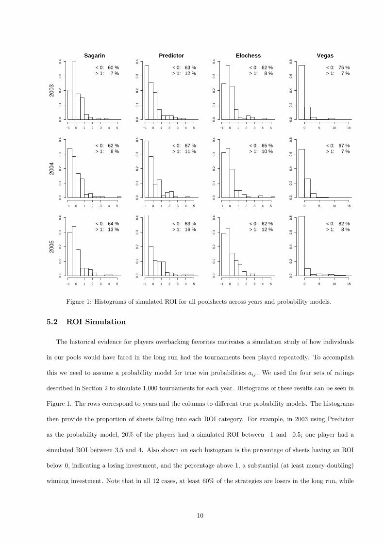
Figure 2: Scatterplot of similarity versus log(probability) with ROI indicated by shading, Predictor ratings.

the proportion that double one’s money or better rarely exceeds 15%.

A natural question at this point concerns the differences between those pool sheets consistently near the

top and bottom of the simulated ROI distributions in Figure 1. Figure 2 plots similarity versus log(probability)

using the Predictor rating for the sheets in our dataset. The plotting character indicates the sheet’s year, while

its shading indicates its simulated ROI (with darker shading corresponding to higher ROI). The figure suggests

the first requirement for a high ROI is to have a relatively high probability, since there are very few dark points

with log-probability less than –30. However, low similarity also appears to be a general characteristic of high

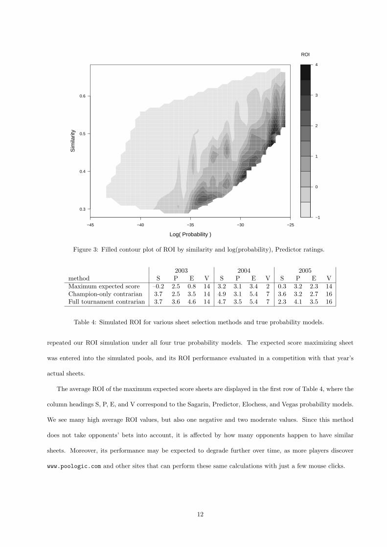
ROI sheets. This relationship is further clarified by the filled contour plot in Figure 3, which indicates that

given a sheet’s log-probability, low similarity tends to maximize ROI, and also that given a sheet’s similarity,

high probability tends to maximize ROI.

5.3 Expected Score Maximization

As mentioned above, most previous work in this area has focused on identifying sheets that maximize

expected score. To further illustrate that this method may not deliver a sheet with high expected ROI, we

derived the maximizing sheet for each year using the algorithm of Kaplan and Garstka (2001). We then

11

−1

0

1

2

3

4

ROI

−45 −40 −35 −30 −25

0.3

0.4

0.5

0.6

Log( Probability )

Sim

ilarit

y

Figure 3: Filled contour plot of ROI by similarity and log(probability), Predictor ratings.

2003 2004 2005method S P E V S P E V S P E VMaximum expected score –0.2 2.5 0.8 14 3.2 3.1 3.4 2 0.3 3.2 2.3 14Champion-only contrarian 3.7 2.5 3.5 14 4.9 3.1 5.4 7 3.6 3.2 2.7 16Full tournament contrarian 3.7 3.6 4.6 14 4.7 3.5 5.4 7 2.3 4.1 3.5 16

Table 4: Simulated ROI for various sheet selection methods and true probability models.

repeated our ROI simulation under all four true probability models. The expected score maximizing sheet

was entered into the simulated pools, and its ROI performance evaluated in a competition with that year’s

actual sheets.

The average ROI of the maximum expected score sheets are displayed in the first row of Table 4, where the

column headings S, P, E, and V correspond to the Sagarin, Predictor, Elochess, and Vegas probability models.

We see many high average ROI values, but also one negative and two moderate values. Since this method

does not take opponents’ bets into account, it is affected by how many opponents happen to have similar

sheets. Moreover, its performance may be expected to degrade further over time, as more players discover

www.poologic.com and other sites that can perform these same calculations with just a few mouse clicks.

12

2003Team A S P E VKentucky 58 18 15 19 15Arizona 15 13 13 12 12Kansas 9 10 19 6 0 POklahoma 8 6 5 6 4Illinois 5 2 3 2 0Texas 5 9 7 9 40 VSyracuse 4 8 4 15 1 EFlorida 3 5 4 4 2Pittsburgh 2 11 11 9 2 SDayton 1 0 0 1 0Indiana 1 0 0 0 0Maryland 1 2 4 1 0Louisville 1 4 6 2 4

Other 0 26 23 27 32

2004Team A S P E VUConn 30 24 12 23 5Kentucky 27 6 8 6 29OK State 23 14 8 15 4Duke 19 24 31 18 24 PStanford 12 5 5 6 13Gonzaga 5 5 9 3 17Pitt 4 4 3 9 0Georgia Tech 3 9 10 9 2St. Joseph’s 3 15 12 18 17 SEVTexas 3 3 3 3 0Wisconsin 2 2 3 1 0Syracuse 2 1 0 2 0Michigan St. 1 0 0 0 0Wake Forest 1 2 4 2 7Cincinnati 1 1 5 1 2North Carolina 1 2 4 1 2Maryland 1 1 2 1 3Other 0 19 19 18 13

2005Team A S P E VIllinois 83 31 15 67 18North Carolina 38 32 56 20 51 PDuke 13 18 21 13 3Oklahoma St. 12 10 14 4 0Washington 3 11 7 9 37 EVWake Forest 3 14 10 7 28 SKentucky 3 7 4 8 1Gonzaga 2 1 0 2 0Florida 2 2 4 1 0Michigan St. 2 3 3 3 0Boston College 1 1 0 2 0Arizona 1 3 1 4 0Georgia Tech 1 1 2 0 0Louisville 1 6 10 6 1Kansas 1 6 4 2 0Oklahoma 1 5 5 2 22

Other 0 15 11 17 5

Table 5: Actual (A) versus expected (S, P, E, V) champion picks, 2003-2005 pool data.

5.4 Champion-only Contrarian

In a first attempt to increase our average ROI, we will use information about how our 2003–2005 opponents

bet to pick an “underbet champion” (i.e., the championship game’s most underappreciated team) in each year,

and then simply use maximum expected score to fill in the remainder of our sheet. Similar to elsewhere in

this section, our calculations may vary with the true probability model we are assuming. If the resulting

champion-only contrarian sheet does not perform well, this bodes ill for the practical setting where opponent

behavior can only be estimated.

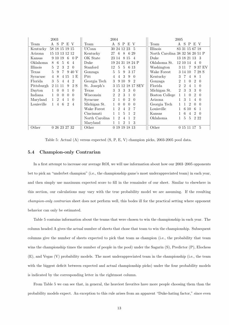
Table 5 contains information about the teams that were chosen to win the championship in each year. The

column headed A gives the actual number of sheets that chose that team to win the championship. Subsequent

columns give the number of sheets expected to pick that team as champion (i.e., the probability that team

wins the championship times the number of people in the pool) under the Sagarin (S), Predictor (P), Elochess

(E), and Vegas (V) probability models. The most underappreciated team in the championship (i.e., the team

with the biggest deficit between expected and actual championship picks) under the four probability models

is indicated by the corresponding letter in the rightmost column.

From Table 5 we can see that, in general, the heaviest favorites have more people choosing them than the

probability models expect. An exception to this rule arises from an apparent “Duke-hating factor,” since even

13

when Duke is a favorite it tends not to be overbacked. However, Kentucky seems overappreciated in 2003 and

2004, and the extreme devotion to Illinois in 2005 is not totally unexpected in this Chicago-based pool.

Returning then to our quest for a high average ROI sheet, we simulate ROI for a sheet taking the most

underbet champion and then score-maximizing for all previous games subject to this constraint. The results are

displayed in Table 4 in the row marked “champion-only contrarian.” Comparing these results to the maximum

expected score results, we can see that in 4 of 12 cases the average ROI is the same, and in the remaining 8

cases it is higher for the underbet champion sheet. Surprisingly, the average ROI under the Predictor model is

the same in all 3 years using both maximum expected score and champion-only contrarian methods, since the

underappreciated champion happens to also be the most probable champion in each year. However, in all but

one of the remaining cases, the contrarian approach offers an often substantial improvement. These results

indicate that if we know how our opponents select a champion, we may be able to improve our expected ROI.

5.5 Full Tournament Contrarian

The next logical question to ask is whether we can make further ROI gains by using the knowledge of how

our opponents bet in all rounds, rather than just the championship. To do this we look at our underbetness

statistic, given in (2). To determine a sheet we developed an algorithm that mimicks human betting behavior

somewhat by working backwards from the championship. Beginning with r = R, it chooses the team t with

the largest underbetness statistic through this final round, UR(t), as the champion. Now, for any round r, in

moving back to round r−1 there are 2R−r games to predict. But half of these games are determined by teams

who have already been selected by the algorithm as winners in later rounds. The other half are determined

by maximizing Ur−1(t) over all possible winners of that game. Letting r range from R back down to 1 then

determines the entire sheet.

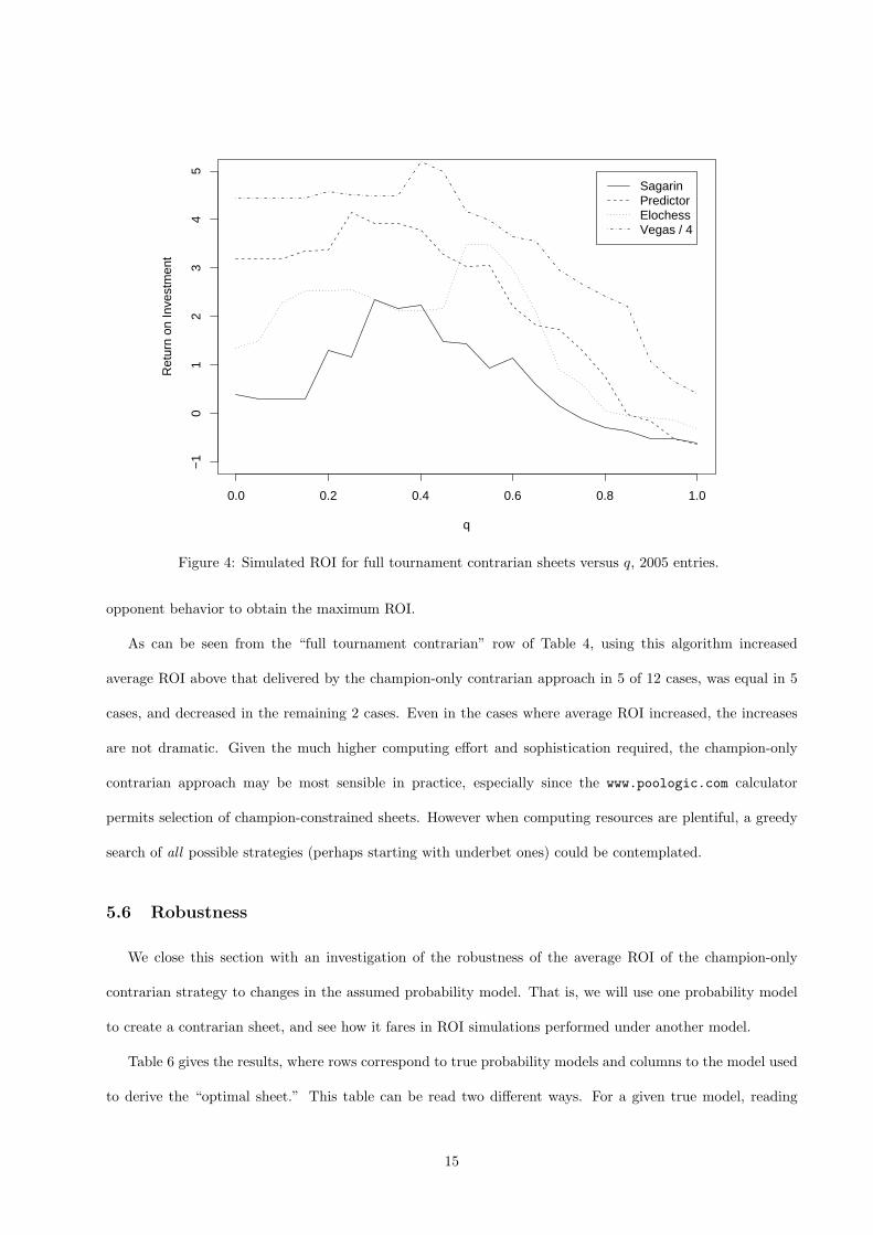
Looking again at (2), values of the relative weight q increasing from 0 to 1 by steps of 0.05 were tried

with the maximum ROI recorded for each. The value of q that provided the maximum average ROI varied

depending on the year and the probability model used. Figure 4 shows the results for 2005 for our values of

q. As the legend indicates, the ROI for Vegas was divided by 4 to keep it on roughly the same scale as the

other ratings. A q of 0 indicates we are not considering opponent behavior at all, while increasing q indicates

progressively more weight on contrarian thinking. Since each rating gives a curve with a maximum ROI at

q values between 0.2 and 0.6, we can see that it is important to use knowledge of both team abilities and

14

0.0 0.2 0.4 0.6 0.8 1.0

−1

01

23

45

q

Ret

urn

on In

vest

men

t

SagarinPredictorElochessVegas / 4

Figure 4: Simulated ROI for full tournament contrarian sheets versus q, 2005 entries.

opponent behavior to obtain the maximum ROI.

As can be seen from the “full tournament contrarian” row of Table 4, using this algorithm increased

average ROI above that delivered by the champion-only contrarian approach in 5 of 12 cases, was equal in 5

cases, and decreased in the remaining 2 cases. Even in the cases where average ROI increased, the increases

are not dramatic. Given the much higher computing effort and sophistication required, the champion-only

contrarian approach may be most sensible in practice, especially since the www.poologic.com calculator

permits selection of champion-constrained sheets. However when computing resources are plentiful, a greedy

search of all possible strategies (perhaps starting with underbet ones) could be contemplated.

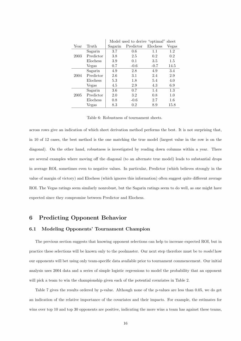
5.6 Robustness

We close this section with an investigation of the robustness of the average ROI of the champion-only

contrarian strategy to changes in the assumed probability model. That is, we will use one probability model

to create a contrarian sheet, and see how it fares in ROI simulations performed under another model.

Table 6 gives the results, where rows correspond to true probability models and columns to the model used

to derive the “optimal sheet.” This table can be read two different ways. For a given true model, reading

15

Model used to derive “optimal” sheetYear Truth Sagarin Predictor Elochess Vegas

Sagarin 3.7 0.6 1.1 1.22003 Predictor 3.8 2.5 0.2 0.2

Elochess 3.9 0.1 3.5 1.5Vegas 0.7 -0.6 -0.7 14.5Sagarin 4.9 2.8 4.9 3.4

2004 Predictor 2.6 3.1 2.4 2.9Elochess 5.3 1.8 5.4 4.0Vegas 4.5 2.9 4.3 6.9Sagarin 3.6 0.7 1.4 1.3

2005 Predictor 2.0 3.2 0.8 1.0Elochess 0.8 -0.6 2.7 1.6Vegas 8.3 0.2 8.9 15.8

Table 6: Robustness of tournament sheets.

across rows give an indication of which sheet derivation method performs the best. It is not surprising that,

in 10 of 12 cases, the best method is the one matching the true model (largest value in the row is on the

diagonal). On the other hand, robustness is investigated by reading down columns within a year. There

are several examples where moving off the diagonal (to an alternate true model) leads to substantial drops

in average ROI, sometimes even to negative values. In particular, Predictor (which believes strongly in the

value of margin of victory) and Elochess (which ignores this information) often suggest quite different average

ROI. The Vegas ratings seem similarly nonrobust, but the Sagarin ratings seem to do well, as one might have

expected since they compromise between Predictor and Elochess.

6 Predicting Opponent Behavior

6.1 Modeling Opponents’ Tournament Champion

The previous section suggests that knowing opponent selections can help to increase expected ROI, but in

practice these selections will be known only to the poolmaster. Our next step therefore must be to model how

our opponents will bet using only team-specific data available prior to tournament commencement. Our initial

analysis uses 2004 data and a series of simple logistic regressions to model the probability that an opponent

will pick a team to win the championship given each of the potential covariates in Table 2.

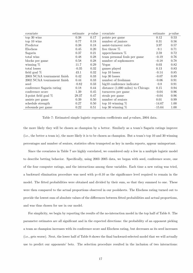
Table 7 gives the results ordered by p-value. Although none of the p-values are less than 0.05, we do get

an indication of the relative importance of the covariates and their impacts. For example, the estimates for

wins over top 10 and top 30 opponents are positive, indicating the more wins a team has against these teams,

16

covariate estimate p-value covariate estimate p-valuetop 30 wins 0.38 0.17 points per game 0.12 0.53top 10 wins 0.77 0.18 number of juniors 0.31 0.56Predictor 0.38 0.18 assist-turnover ratio 3.97 0.57Elochess 0.45 0.20 free throw % –9.1 0.71Sagarin 0.37 0.21 upperclassmen % 2.59 0.72total wins 0.48 0.28 team personal fouls per game –0.19 0.76blocks per game 0.58 0.28 number of sophomores –0.18 0.78winning % 11.7 0.29 Vegas 0.03 0.82total losses –0.35 0.32 games played 0.13 0.83field goal % 43.1 0.32 top 10 losses –0.14 0.852003 NCAA tournament finish 0.42 0.33 top 30 losses –0.07 0.892002 NCAA tournament finish 0.44 0.33 number of freshman –0.06 0.91seed –0.82 0.33 big10 conference indicator –0.8 0.91conference Sagarin rating 0.18 0.44 distance (1,000 miles) to Chicago 0.15 0.94conference score 1.39 0.45 turnovers per game –0.04 0.963-point field goal % 29.37 0.47 steals per game –0.04 0.96assists per game 0.39 0.50 number of seniors 0.01 0.99schedule strength 0.27 0.50 top 10 winning % –14.67 1.00rebounds per game 0.22 0.51 top 30 winning % –15.64 1.00

Table 7: Estimated simple logistic regression coefficients and p-values, 2004 data.

the more likely they will be chosen as champion by a bettor. Similarly as a team’s Sagarin ratings improve

(i.e., the better a team is), the more likely it is to be chosen as champion. But a team’s top 10 and 30 winning

percentages and number of seniors, statistics often trumpeted as key in media reports, appear unimportant.

Since the covariates in Table 7 are highly correlated, we considered only a few in a multiple logistic model

to describe betting behavior. Specifically, using 2003–2005 data, we began with seed, conference score, one

of the four computer ratings, and the interactions among these variables. Each time a new rating was tried,

a backward elimination procedure was used with p=0.10 as the significance level required to remain in the

model. The fitted probabilities were obtained and divided by their sum, so that they summed to one. These

were then compared to the actual proportions observed in our poolsheets. The Elochess rating turned out to

provide the lowest sum of absolute values of the differences between fitted probabilities and actual proportions,

and was thus chosen for use in our model.

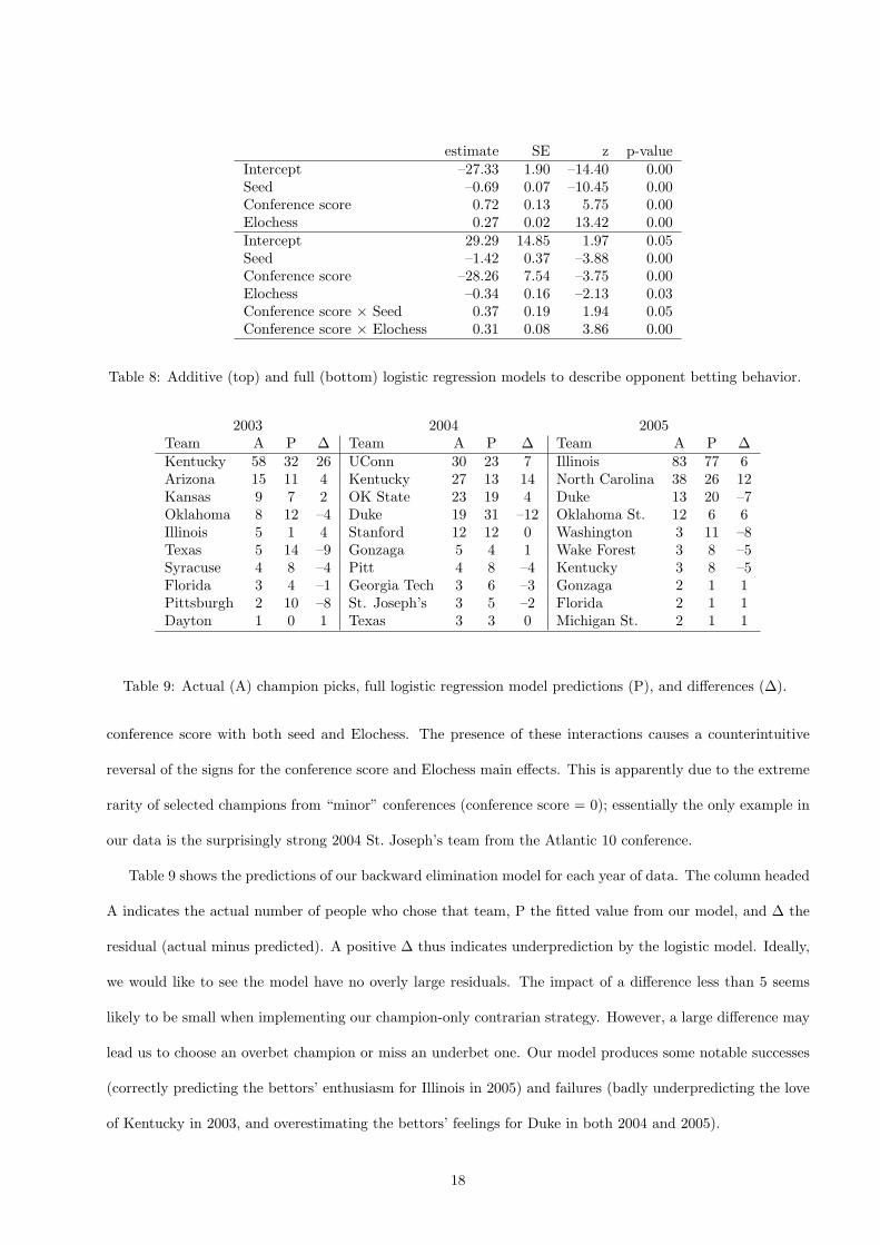
For simplicity, we begin by reporting the results of the no-interaction model in the top half of Table 8. The

parameter estimates are all significant and in the expected directions: the probability of an opponent picking

a team as champion increases with its conference score and Elochess rating, but decreases as its seed increases

(i.e., gets worse). Next, the lower half of Table 8 shows the final backward-selected model that we will actually

use to predict our opponents’ bets. The selection procedure resulted in the inclusion of two interactions:

17

estimate SE z p-valueIntercept –27.33 1.90 –14.40 0.00Seed –0.69 0.07 –10.45 0.00Conference score 0.72 0.13 5.75 0.00Elochess 0.27 0.02 13.42 0.00Intercept 29.29 14.85 1.97 0.05Seed –1.42 0.37 –3.88 0.00Conference score –28.26 7.54 –3.75 0.00Elochess –0.34 0.16 –2.13 0.03Conference score × Seed 0.37 0.19 1.94 0.05Conference score × Elochess 0.31 0.08 3.86 0.00

Table 8: Additive (top) and full (bottom) logistic regression models to describe opponent betting behavior.

2003 2004 2005Team A P ∆ Team A P ∆ Team A P ∆Kentucky 58 32 26 UConn 30 23 7 Illinois 83 77 6Arizona 15 11 4 Kentucky 27 13 14 North Carolina 38 26 12Kansas 9 7 2 OK State 23 19 4 Duke 13 20 –7Oklahoma 8 12 –4 Duke 19 31 –12 Oklahoma St. 12 6 6Illinois 5 1 4 Stanford 12 12 0 Washington 3 11 –8Texas 5 14 –9 Gonzaga 5 4 1 Wake Forest 3 8 –5Syracuse 4 8 –4 Pitt 4 8 –4 Kentucky 3 8 –5Florida 3 4 –1 Georgia Tech 3 6 –3 Gonzaga 2 1 1Pittsburgh 2 10 –8 St. Joseph’s 3 5 –2 Florida 2 1 1Dayton 1 0 1 Texas 3 3 0 Michigan St. 2 1 1

Table 9: Actual (A) champion picks, full logistic regression model predictions (P), and differences (∆).

conference score with both seed and Elochess. The presence of these interactions causes a counterintuitive

reversal of the signs for the conference score and Elochess main effects. This is apparently due to the extreme

rarity of selected champions from “minor” conferences (conference score = 0); essentially the only example in

our data is the surprisingly strong 2004 St. Joseph’s team from the Atlantic 10 conference.

Table 9 shows the predictions of our backward elimination model for each year of data. The column headed

A indicates the actual number of people who chose that team, P the fitted value from our model, and ∆ the

residual (actual minus predicted). A positive ∆ thus indicates underprediction by the logistic model. Ideally,

we would like to see the model have no overly large residuals. The impact of a difference less than 5 seems

likely to be small when implementing our champion-only contrarian strategy. However, a large difference may

lead us to choose an overbet champion or miss an underbet one. Our model produces some notable successes

(correctly predicting the bettors’ enthusiasm for Illinois in 2005) and failures (badly underpredicting the love

of Kentucky in 2003, and overestimating the bettors’ feelings for Duke in both 2004 and 2005).

18

Model used to derive “optimal” sheetPredicted champion-only contrarian Maximum expected score

Year Truth Sagarin Predictor Elochess Vegas Sagarin Predictor Elochess VegasSagarin 0.6 0.6 1.1 1.2 –0.2 0.6 0.1 1.2

2003 Predictor 1.6 2.5 0.2 0.2 –0.5 2.5 –0.2 0.2Elochess 0.2 0.1 3.5 1.5 0.0 0.1 0.8 1.5Vegas 1.1 –0.6 –0.7 14.5 –0.2 –0.6 –0.9 14.5Sagarin 4.9 4.6 4.9 –0.5 3.2 2.8 3.2 –0.5

2004 Predictor 2.6 3.5 2.4 –0.1 0.8 3.1 0.7 –0.1Elochess 5.3 4.7 5.4 –0.7 3.3 1.8 3.4 –0.7Vegas 4.5 4.6 4.3 2.4 0.6 2.9 0.5 2.4Sagarin 0.3 0.7 1.7 1.3 0.3 0.7 0.1 2.1

2005 Predictor 1.0 3.2 2.7 1.0 1.0 3.2 –0.4 3.1Elochess 0.1 –0.6 1.4 1.6 0.1 –0.6 2.3 1.3Vegas 0.9 0.2 –0.5 15.8 0.9 0.2 –0.3 13.7

Table 10: Average ROI using Maximum Expected Score and Predicted champion-only contrarian.

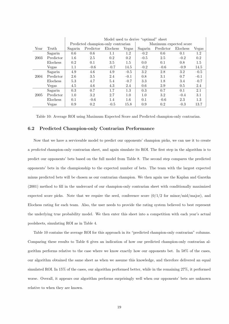
6.2 Predicted Champion-only Contrarian Performance

Now that we have a serviceable model to predict our opponents’ champion picks, we can use it to create

a predicted champion-only contrarian sheet, and again simulate its ROI. The first step in the algorithm is to

predict our opponents’ bets based on the full model from Table 8. The second step compares the predicted

opponents’ bets in the championship to the expected number of bets. The team with the largest expected

minus predicted bets will be chosen as our contrarian champion. We then again use the Kaplan and Garstka

(2001) method to fill in the undercard of our champion-only contrarian sheet with conditionally maximized

expected score picks. Note that we require the seed, conference score (0/1/2 for minor/mid/major), and

Elochess rating for each team. Also, the user needs to provide the rating system believed to best represent

the underlying true probability model. We then enter this sheet into a competition with each year’s actual

poolsheets, simulating ROI as in Table 4.

Table 10 contains the average ROI for this approach in its “predicted champion-only contrarian” columns.

Comparing these results to Table 6 gives an indication of how our predicted champion-only contrarian al-

gorithm performs relative to the case where we know exactly how our opponents bet. In 58% of the cases,

our algorithm obtained the same sheet as when we assume this knowledge, and therefore delivered an equal

simulated ROI. In 15% of the cases, our algorithm performed better, while in the remaining 27%, it performed

worse. Overall, it appears our algorithm performs surprisingly well when our opponents’ bets are unknown

relative to when they are known.

19

Table 10 also contains the average ROI for the maximum expected score method. In 42% of the cases, our

algorithm obtained the same sheet as the maximum expected score sheet. In 50% of the cases our algorithm

performed better and in only 8% of the cases it performed worse than the maximum expected score sheet.

Thus despite its imperfect knowledge of our opponents’ bets, our predicted champion-only contrarian algorithm

again appears to outperform the maximum expected score algorithm.

7 Discussion

In this article we have presented contrarian algorithms that improve simulated ROI over strategies that

maximize expected score in NCAA tournament pools with standard scoring schemes. Our champion-only

contrarian approach requires only that the user select a contrarian champion, and fill in the rest of his

sheet using maximization of expected score subject to this constraint, free software for which is available at

www.poologic.com. The pre-tournament prediction of a contrarian champion may be done formally using

logistic regression, which in turn requires the user to collect seed, computer rating, and conference score

information on all teams in the tournament. Our evaluations to date have implicitly used partial opponent

betting information, since our logistic regression parameter estimates were computed using data from the same

years for which we were trying to create contrarian sheets. As such, the true test of our method will come in

future years, when opponents’ champion selections will be unknown.

A less formal contrarian strategy would avoid logistic regression and simply make an educated guess about

which team will be the most underbet in the championship. With this educated guess, one could again use

the poologic calculator, and thus obtain a good sheet with minimal effort. One ad hoc rule for most pools is

to avoid the heaviest favorites (say, the two or three #1 seeds with the highest AP rankings), since they are

typically overbacked. Another ad hoc rule is to avoid local teams. In 2005, we correctly guessed bettors in our

Chicago-based pool would overback Illinois since they were both a “local” team (they received heavy media

coverage in Chicago) and one of the two heaviest favorites. Other ad hoc rules may arise from experience

with one’s own pool; we will certainly be looking carefully at Duke in future years since our opponents seem

to dislike them.

We hasten to mention a few features common to office pools that our analysis has not explicitly considered.

For example, many pools award extra prizes to the top sheet(s) after Round 2 and Round 4, or perhaps a

20

“booby prize” (often a refund of the entry fee) to the sheet with the lowest score at the end of the tournament.

Our work assumes the effect of such prizes on our strategy to be negligible. Also, some pools allow bettors to

enter more than one sheet in the pool, each sheet having its own picks and entry fee. This offers a player a way

to “better cover” the probability space of probable outcomes. While we did not consider this feature in order

to make our results more generally applicable, such a feature clearly opens a wide range of new questions

regarding both the optimal number of sheets to enter and how their champions and undercards should be

selected. Another area requiring further consideration is the effect of the size of the pool on the optimal

contrarian strategy. Our pool was medium-sized, having 113, 138, and 167 participants in the three years,

respectively. Our contrarian strategies seem to work well in pools of this size, but many office pools are much

smaller, while many online pools are enormously larger, having thousands or even millions of entries. Intuition

(and previous work by Clair and Letscher, 2005) suggests the value of contrarian thinking may increase with

pool size, since the bettors’ overbacking of favorites will cause the maximum expected score sheet’s return to

drop as more bettors are added.

Regardless of the strategy used to determine one’s sheet in a pool, a guess at the true probability model

is required. The return of our strategies will obviously drop as these guesses depart from the truth. In our

case, we rely on rating systems (especially Sagarin) that do not attempt to account for many relevant factors,

such as autocorrelation in game performance, injuries to key players, specific “matchup” problems, and so on.

Thus while reliance on ratings can decrease our bias toward teams we have seen play more than others, they

cannot fully replace expert knowledge of the teams and the sport itself.

Finally, although we believe contrarian strategies provide for a potential positive return on investment, we

must confess that we have not actually realized any dividends to date. Underbet champion St. Joseph’s did not

quite make the Final Four in 2004 (losing to Oklahoma State on a three-pointer at the buzzer), and 2005 was

certainly not the year to be contrarian (with the two heavy favorites, North Carolina and Illinois, successfully

arriving at the championship game). Nevertheless, we look forward to future years when the heaviest favorites

do lose, and the advantage to straying from the crowd becomes apparent.

References

Breiter, D.J. and Carlin, B.P. (1997), “How to play office pools if you must,” Chance, 10, 324–345.

21

Carlin, B.P. (1996), “Improved NCAA basketball tournament modeling via point spread and team strength

information,” The American Statistician, 50, 39–43.

Clair, B. and Letscher, D. (2005), “Optimal strategies for sports betting pools,” technical report, De-

partment of Mathematics, Saint Louis University.

Kaplan, E.H. and Garstka, S.J. (2001), “March madness and the office pool,” Management Science, 47,

369–382

Metrick, A. (1996), “March madness? Strategic behavior in NCAA basketball tournament betting pools,”

Journal of Economic Behavior & Organization, 96, 159–172.

Schwertman, N.C., McCready, T.A. and Howard, L. (1991), “Probability models for the NCAA

regional basketball tournaments,” The American Statistician, 45, 35–38.

Schwertman, N.C., Schenk, K.L. and Holbrook, B.C. (1996), “More probability models for the NCAA

regional basketball tournaments,” The American Statistician, 50, 34–38.

Stern, H. (1991), “On the probability of winning a football game,” The American Statistician, 45, 179–183.

22