Identification of Continuous-time Models from Sampled...
44
Hugues Garnier • Liuping Wang Editors Identification of Continuous-time Models from Sampled Data 123
Transcript of Identification of Continuous-time Models from Sampled...
Hugues Garnier • Liuping Wang Editors
Identification of Continuous-time Models from Sampled Data
123
Hugues Garnier, PhD Centre de Recherche en Automatique
de Nancy (CRAN) Nancy-Université CNRS Faculté des Sciences et Techniques 54506 Vandoeuvre-les-Nancy France
Liuping Wang, PhD RMIT University School of Electrical and Computing
Engineering Swanston Street Melbourne 3000 Victoria Australia
ISBN 978-1-84800-160-2 e-ISBN 978-1-84800-161-9
DOI 10.1007/978-1-84800-161-9
Advances in Industrial Control series ISSN 1430-9491
British Library Cataloguing in Publication Data Identification of continuous-time models from sampled data. - (Advances in industrial control) 1. Linear time invariant systems - Mathematical models - Congresses 2. Automatic control - Congresses I. Garnier, Hugues II. Wang, Liuping 629.8'32 ISBN-13: 9781848001602
Library of Congress Control Number: 2007942577
© 2008 Springer-Verlag London Limited
MATLAB® and Simulink® are registered trademarks of The MathWorks, Inc., 3 Apple Hill Drive, Natick,MA 01760-2098, USA. http://www.mathworks.com
Apart from any fair dealing for the purposes of research or private study, or criticism or review, as permitted under the Copyright, Designs and Patents Act 1988, this publication may only be reproduced, stored ortransmitted, in any form or by any means, with the prior permission in writing of the publishers, or in the case of reprographic reproduction in accordance with the terms of licences issued by the CopyrightLicensing Agency. Enquiries concerning reproduction outside those terms should be sent to the publishers.
The use of registered names, trademarks, etc. in this publication does not imply, even in the absence of a specific statement, that such names are exempt from the relevant laws and regulations and therefore free forgeneral use.
The publisher makes no representation, express or implied, with regard to the accuracy of the information contained in this book and cannot accept any legal responsibility or liability for any errors or omissions thatmay be made.
Cover design: eStudio Calamar S.L., Girona, Spain
Printed on acid-free paper
9 8 7 6 5 4 3 2 1 springer.com
9
The CONTSID Toolbox: A Software Supportfor Data-based Continuous-time Modelling
Hugues Garnier1, Marion Gilson1, Thierry Bastogne1 and Michel Mensler2
1 Nancy-Universite, CNRS, France2 Direction de la Recherche, Etudes Avancees, Materiaux - Renault, France
9.1 Introduction
This chapter describes the continuous-time system identification (CONTSID)toolbox for MATLAB�, which supports continuous-time (CT) transfer func-tion and state-space model identification directly from regularly or irregularlytime-domain sampled data, without requiring the determination of a discrete-time (DT) model. The motivation for developing the CONTSID toolbox wasfirst to fill in a gap, since no software support was available to serve the causeof direct time-domain identification of continuous-time linear models but alsoto provide the potential user with a platform for testing and evaluating thesedata-based modelling techniques. The CONTSID toolbox was first releasedin 1999 [15]. It has gone through several updates, some of which have beenreported at recent symposia [11, 12, 16]. The key features of the CONTSIDtoolbox can be summarised as follows:
• it supports most of the time-domain methods developed over the last thirtyyears [17] for identifying linear dynamic continuous-time parametric mo-dels from measured input/output sampled data;
• it provides transfer function and state-space model identification methodsfor single-input single-output (SISO) and multiple-input multiple-output(MIMO) systems, including both traditional and more recent approaches;
• it can handle irregularly sampled data in a straightforward way;• it may be seen as an add-on to the system identification (SID) toolbox for
MATLAB� [26]. To facilitate its use, it has been given a similar setup tothe SID toolbox;
• it provides a flexible graphical user interface (GUI) that lets the user anal-yse the experimental data, identify and evaluate models in an easy way.
The chapter is organised in the following way. Section 9.2 outlines the mainsteps of the procedure for direct continuous-time model identification. Anoverview of the identification tools available in the toolbox is given in Sec-tion 9.3. An introductory example to the command mode along with a brief
250 H. Garnier et al.
description of the GUI are then presented in Section 9.4. In Section 9.5, the ad-vantages of CT model identification approaches are discussed and illustrated.A few successful application results from real-life process data are describedin Section 9.6. Finally, Section 9.7 presents conclusions of the chapter andhighlights future developments for the toolbox.
9.2 General Procedure for Continuous-time ModelIdentification
The procedure to directly determine a continuous-time model of a dynamicalsystem directly from observed time-domain input/output data is similar tothe general approach used for traditional DT model identification and involvesthree basic ingredients:
• the time-domain sampled input/output data;• a set of candidate models (the model structure);• a criterion to select a particular model in the set, based on the information
in the data (the parametric model estimation method).
The identification procedure consists then in repeatedly selecting a modelstructure, computing the best model in the chosen structure, and evaluat-ing the identified model. More precisely, the iterative procedure involves thefollowing steps:
1. Design an experiment and collect time-domain input/output data fromthe process to be identified.
2. Examine the data. Remove trends and outliers, and select useful portionsof the original data.
3. Select and define a model structure (a set of candidate system descrip-tions) within which a model is to be estimated.
4. Estimate the parameters in the chosen model structure according to theinput/output data and a given criterion of fit.
5. Examine the finally estimated model properties.
If the model is good enough, then stop; otherwise go back to Step 3 and tryanother model set. Possibly also try other estimation methods (Step 4) orwork further on the input/output data (Steps 1 and 2).As described in the following section, the CONTSID toolbox includes toolsfor applying the general data-based modelling procedure summarised above.
9.3 Overview of the CONTSID Toolbox
9.3.1 Parametric Model Estimation
The CONTSID toolbox offers a variety of parametric model estimation meth-ods for the most common input/output and state-space model structures.
9 The CONTSID toolbox for MATLAB� 251
CT ARX Models
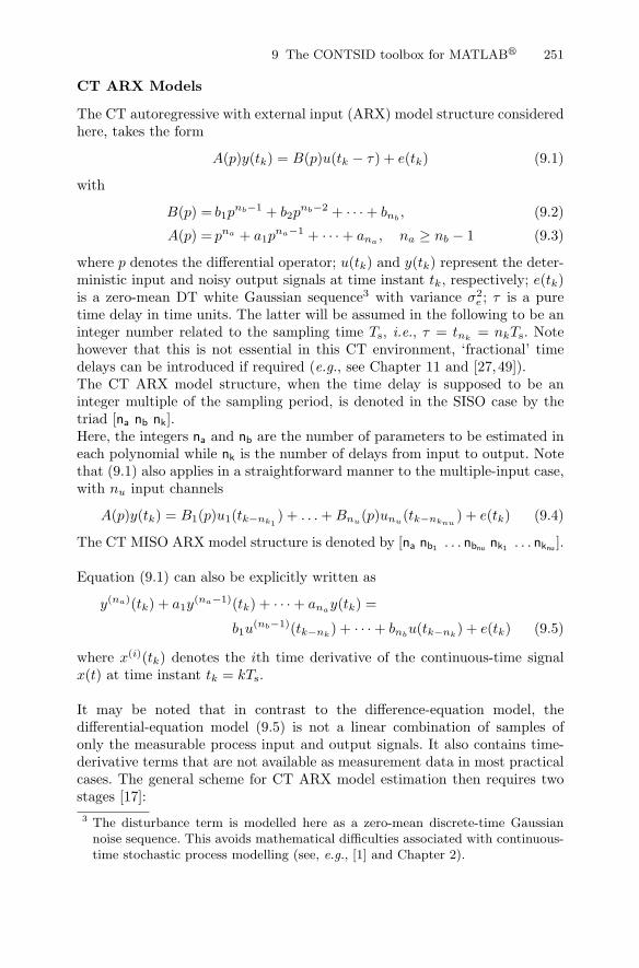
The CT autoregressive with external input (ARX) model structure consideredhere, takes the form
A(p)y(tk) = B(p)u(tk − τ) + e(tk) (9.1)
with
B(p) = b1pnb−1 + b2p
nb−2 + · · · + bnb, (9.2)
A(p) = pna + a1pna−1 + · · · + ana
, na ≥ nb − 1 (9.3)
where p denotes the differential operator; u(tk) and y(tk) represent the deter-ministic input and noisy output signals at time instant tk, respectively; e(tk)is a zero-mean DT white Gaussian sequence3 with variance σ2
e ; τ is a puretime delay in time units. The latter will be assumed in the following to be aninteger number related to the sampling time Ts, i.e., τ = tnk
= nkTs. Notehowever that this is not essential in this CT environment, ‘fractional’ timedelays can be introduced if required (e.g., see Chapter 11 and [27,49]).The CT ARX model structure, when the time delay is supposed to be aninteger multiple of the sampling period, is denoted in the SISO case by thetriad [na nb nk].Here, the integers na and nb are the number of parameters to be estimated ineach polynomial while nk is the number of delays from input to output. Notethat (9.1) also applies in a straightforward manner to the multiple-input case,with nu input channels
A(p)y(tk) = B1(p)u1(tk−nk1) + . . . + Bnu
(p)unu(tk−nknu
) + e(tk) (9.4)
The CT MISO ARX model structure is denoted by [na nb1 . . . nbnu nk1 . . . nknu ].
Equation (9.1) can also be explicitly written as
y(na)(tk) + a1y(na−1)(tk) + · · · + ana
y(tk) =
b1u(nb−1)(tk−nk
) + · · · + bnbu(tk−nk
) + e(tk) (9.5)
where x(i)(tk) denotes the ith time derivative of the continuous-time signalx(t) at time instant tk = kTs.
It may be noted that in contrast to the difference-equation model, thedifferential-equation model (9.5) is not a linear combination of samples ofonly the measurable process input and output signals. It also contains time-derivative terms that are not available as measurement data in most practicalcases. The general scheme for CT ARX model estimation then requires twostages [17]:3 The disturbance term is modelled here as a zero-mean discrete-time Gaussian
noise sequence. This avoids mathematical difficulties associated with continuous-time stochastic process modelling (see, e.g., [1] and Chapter 2).
252 H. Garnier et al.
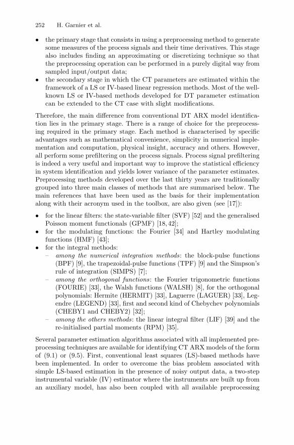
• the primary stage that consists in using a preprocessing method to generatesome measures of the process signals and their time derivatives. This stagealso includes finding an approximating or discretizing technique so thatthe preprocessing operation can be performed in a purely digital way fromsampled input/output data;
• the secondary stage in which the CT parameters are estimated within theframework of a LS or IV-based linear regression methods. Most of the well-known LS or IV-based methods developed for DT parameter estimationcan be extended to the CT case with slight modifications.
Therefore, the main difference from conventional DT ARX model identifica-tion lies in the primary stage. There is a range of choice for the preprocess-ing required in the primary stage. Each method is characterised by specificadvantages such as mathematical convenience, simplicity in numerical imple-mentation and computation, physical insight, accuracy and others. However,all perform some prefiltering on the process signals. Process signal prefilteringis indeed a very useful and important way to improve the statistical efficiencyin system identification and yields lower variance of the parameter estimates.Preprocessing methods developed over the last thirty years are traditionallygrouped into three main classes of methods that are summarised below. Themain references that have been used as the basis for their implementationalong with their acronym used in the toolbox, are also given (see [17]):
• for the linear filters: the state-variable filter (SVF) [52] and the generalisedPoisson moment functionals (GPMF) [18,42];
• for the modulating functions: the Fourier [34] and Hartley modulatingfunctions (HMF) [43];
• for the integral methods:– among the numerical integration methods: the block-pulse functions
(BPF) [9], the trapezoidal-pulse functions (TPF) [9] and the Simpson’srule of integration (SIMPS) [7];
– among the orthogonal functions: the Fourier trigonometric functions(FOURIE) [33], the Walsh functions (WALSH) [8], for the orthogonalpolynomials: Hermite (HERMIT) [33], Laguerre (LAGUER) [33], Leg-endre (LEGEND) [33], first and second kind of Chebychev polynomials(CHEBY1 and CHEBY2) [32];
– among the others methods: the linear integral filter (LIF) [39] and there-initialised partial moments (RPM) [35].
Several parameter estimation algorithms associated with all implemented pre-processing techniques are available for identifying CT ARX models of the formof (9.1) or (9.5). First, conventional least squares (LS)-based methods havebeen implemented. In order to overcome the bias problem associated withsimple LS-based estimation in the presence of noisy output data, a two-stepinstrumental variable (IV) estimator where the instruments are built up froman auxiliary model, has also been coupled with all available preprocessing
9 The CONTSID toolbox for MATLAB� 253
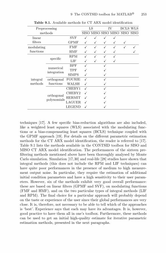
Table 9.1. Available methods for CT ARX model identification
Preprocessing LS IV BCLS WLS
methods SISO MISO SISO MISO SISO SISO
linearfilters
SVF � � � �GPMF � � � � �
modulatingfunctions
FMF � � � � � �HMF � � � � �
integralmethods
specificRPM � � � �LIF � � � �
numericalintegration
BPF � �TPF � �
SIMPS � �orthogonalfunctions
FOURIE � �WALSH � �
orthogonalpolynomials
CHEBY1 � �CHEBY2 � �HERMIT � �LAGUER � �LEGEND � �
techniques [17]. A few specific bias-reduction algorithms are also included,like a weighted least squares (WLS) associated with the modulating func-tions or a bias-compensating least squares (BCLS) technique coupled withthe GPMF approach [19]. For details on the different parametric estimationmethods for the CT ARX model identification, the reader is referred to [17].Table 9.1 lists the methods available in the CONTSID toolbox for SISO andMISO CT ARX model identification. The performances of the sixteen pre-filtering methods mentioned above have been thoroughly analysed by MonteCarlo simulation. Simulation [17,30] and real-life [28] studies have shown thatintegral methods (this does not include the RPM and LIF techniques) canhave quite poor performances in the presence of medium to high measure-ment output noise. In particular, they require the estimation of additionalinitial condition parameters and have a high sensitivity to their user param-eters. However, six of the methods exhibit very good overall performance:these are based on linear filters (GPMF and SVF), on modulating functions(FMF and HMF), and on the two particular types of integral methods (LIFand RPM). The final choice for a particular approach will probably dependon the taste or experience of the user since their global performances are veryclose. It is, therefore, not necessary to be able to tell which of the approachesis ‘best’. Experience says that each may have its advantages. It is, however,good practice to have them all in one’s toolbox. Furthermore, these methodscan be used to get an initial high-quality estimate for iterative parametricestimation methods, presented in the next paragraphs.
254 H. Garnier et al.
CT Hybrid OE Models
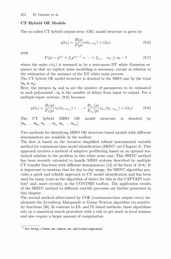
The so-called CT hybrid output-error (OE) model structure is given by
y(tk) =B(p)F (p)
u(tk−nk) + e(tk) (9.6)
withF (p) = pnf + f1p
nf−1 + · · · + fnf, nf ≥ nb − 1 (9.7)
where the noise e(tk) is assumed to be a zero-mean DT white Gaussian se-quence so that no explicit noise modelling is necessary, except in relation tothe estimation of the variance of the DT white noise process.The CT hybrid OE model structure is denoted in the SISO case by the triad[nb nf nk].Here, the integers nb and nf are the number of parameters to be estimatedin each polynomial ; nk is the number of delays from input to output. For amultiple-input systems, (9.6) becomes
y(tk) =B1(p)F1(p)
u1(tk−nk1) + . . . +
Bnu(p)
Fnu(p)
unu(tk−nku
) + e(tk) (9.8)
The CT hybrid MISO OE model structure is denoted by[nb1 . . . nbnu nf1 . . . nfnu nk1 . . . nknu ].
Two methods for identifying MISO OE structure-based models with differentdenominators are available in the toolbox.The first is based on the iterative simplified refined instrumental variablemethod for continuous-time model identification (SRIVC: see Chapter 4). Thisapproach involves a method of adaptive prefiltering based on an optimal sta-tistical solution to the problem in this white noise case. This SRIVC methodhas been recently extended to handle MISO systems described by multipleCT transfer functions with different denominators [13] of the form of (9.8). Itis important to mention that for day-to-day usage, the SRIVC algorithm pro-vides a quick and reliable approach to CT model identification and has beenused for many years as the algorithm of choice for this in the CAPTAIN tool-box4 and, more recently, in the CONTSID toolbox. The application resultsof the SRIVC method to different real-life processes are further presented inthis chapter.The second method abbreviated by COE (continuous-time output error) im-plements the Levenberg–Marquardt or Gauss–Newton algorithm via sensitiv-ity functions [38]. In contrast to LS- and IV-based methods, these algorithmsrely on a numerical search procedure with a risk to get stuck in local minimaand also require a larger amount of computation.
4 See http://www.es.lancs.ac.uk/cres/captain/.
9 The CONTSID toolbox for MATLAB� 255
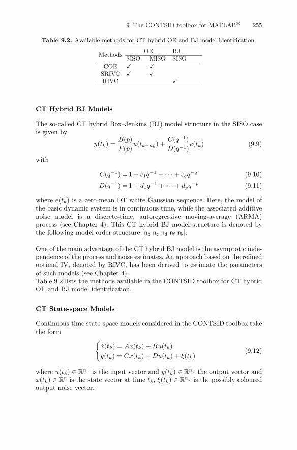
Table 9.2. Available methods for CT hybrid OE and BJ model identification
MethodsOE BJ
SISO MISO SISO
COE � �SRIVC � �RIVC �
CT Hybrid BJ Models
The so-called CT hybrid Box–Jenkins (BJ) model structure in the SISO caseis given by
y(tk) =B(p)F (p)
u(tk−nk) +
C(q−1)D(q−1)
e(tk) (9.9)
with
C(q−1) = 1 + c1q−1 + · · · + cqq
−q (9.10)
D(q−1) = 1 + d1q−1 + · · · + dpq
−p (9.11)
where e(tk) is a zero-mean DT white Gaussian sequence. Here, the model ofthe basic dynamic system is in continuous time, while the associated additivenoise model is a discrete-time, autoregressive moving-average (ARMA)process (see Chapter 4). This CT hybrid BJ model structure is denoted bythe following model order structure [nb nc nd nf nk].
One of the main advantage of the CT hybrid BJ model is the asymptotic inde-pendence of the process and noise estimates. An approach based on the refinedoptimal IV, denoted by RIVC, has been derived to estimate the parametersof such models (see Chapter 4).Table 9.2 lists the methods available in the CONTSID toolbox for CT hybridOE and BJ model identification.
CT State-space Models
Continuous-time state-space models considered in the CONTSID toolbox takethe form
{x(tk) = Ax(tk) + Bu(tk)y(tk) = Cx(tk) + Du(tk) + ξ(tk)
(9.12)
where u(tk) ∈ Rnu is the input vector and y(tk) ∈ R
ny the output vector andx(tk) ∈ R
n is the state vector at time tk, ξ(tk) ∈ Rny is the possibly coloured
output noise vector.
256 H. Garnier et al.
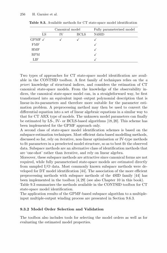
Table 9.3. Available methods for CT state-space model identification
Canonical model Fully parameterised model
LS IV BCLS N4SID
GPMF � � � �FMF �HMF �RPM �LIF �
Two types of approaches for CT state-space model identification are avail-able in the CONTSID toolbox. A first family of techniques relies on the apriori knowledge of structural indices, and considers the estimation of CTcanonical state-space models. From the knowledge of the observability in-dices, the canonical state-space model can, in a straightforward way, be firsttransformed into an equivalent input–output polynomial description that islinear-in-its-parameters and therefore more suitable for the parameter esti-mation problem. A preprocessing method may then be used to convert thedifferential equation into a set of linear algebraic equations in a similar way tothat for CT ARX type of models. The unknown model parameters can finallybe estimated by LS-, IV- or BCLS-based algorithms [18,20]. This scheme hasbeen implemented for the GPMF approach only.A second class of state-space model identification schemes is based on thesubspace-estimation techniques. Most efficient data-based modelling methods,discussed so far, rely on iterative, non-linear optimisation or IV-type methodsto fit parameters in a preselected model structure, so as to best fit the observeddata. Subspace methods are an alternative class of identification methods thatare ‘one-shot’ rather than iterative, and rely on linear algebra.Moreover, these subspace methods are attractive since canonical forms are notrequired, while fully parameterised state-space models are estimated directlyfrom sampled I/O data. Most commonly known subspace methods were de-veloped for DT model identification [44]. The association of the more efficientpreprocessing methods with subspace methods of the 4SID family [44] hasbeen implemented in the toolbox [4, 29] (see also Chapter 10 in this book).Table 9.3 summarises the methods available in the CONTSID toolbox for CTstate-space model identification.The application results of the GPMF-based subspace algorithm to a multiple-input multiple-output winding process are presented in Section 9.6.3.
9.3.2 Model Order Selection and Validation
The toolbox also includes tools for selecting the model orders as well as forevaluating the estimated model properties.
9 The CONTSID toolbox for MATLAB� 257
Model Order Selection
Model order selection is one of the difficult tasks in the system identificationprocedure. A natural way to find the most appropriate model orders is tocompare the results obtained from model structures with different orders anddelays. A model order selection algorithm associated to the SRIVC model es-timation method allows the user to automatically search over a whole range ofdifferent model orders. Two statistical measures are then used for the analysis.The first is the simulation coefficient of determination R2
T , defined as follows
R2T = 1 − σ2
e
σ2y
(9.13)
where σ2e is the variance of the estimated noise e(tk) and σ2
y is the varianceof the measured output y(tk). This should be differentiated from the stan-dard coefficient of determination R2, where the σ2
e in (9.13) is replaced bythe variance of the final noise model residuals σ2. R2
T is clearly a normalisedmeasure of how much of the output variance is explained by the deterministicsystem part of the estimated model. However, it is well known that this mea-sure, on its own, is not sufficient to avoid overparametrisation and identify aparsimonious model, so that other order identification statistics are required.In this regard, because the SRIVC method exploits optimal instrumental vari-able methodology, it is able to utilise the special properties of the instrumentalproduct matrix (IPM) [45, 53]; in particular, the YIC statistic [47] is definedas follows
YIC = logeσ2
σ2y
+ loge{NEVN}; NEVN =1nθ
nθ∑
i=1
pii
θ2i
(9.14)
Here, nθ is the number of estimated parameters; pii is the ith diagonal elementof the block-diagonal SRIVC covariance matrix and so is an estimate of thevariance of the estimated uncertainty on the ith parameter estimate. θ2
i isthe square of the ith SRIVC parameter estimate, so that the ratio pii/θ
2i is a
normalised measure of the uncertainty on the ith parameter estimate.From the definition of R2
T , we see that the first term in the YIC is simplya relative measure of how well the model explains the data: the smaller themodel residuals, the more negative the term becomes. The normalised errorvariance norm (NEVN) term, on the other hand, provides a measure of theconditioning of the IPM, which needs to be inverted when the IV normalequations are solved (see e.g., [46]): if the model is overparameterised, thenit can be shown that the IPM will tend to singularity and, because of its ill-conditioning, the elements of its inverse will increase in value, often by severalorders of magnitude. When this happens, the second term in the YIC tendsto dominate the criterion function, indicating overparametrisation.Although heuristic, the YIC has proven very useful in practical identificationterms. It should not, however, be used as a sole arbiter of model order: rather
258 H. Garnier et al.
the combination of R2T and YIC provides an indication of the best parsimo-
nious models that can be evaluated by other standard statistical measures(e.g., the autocovariance of the model residuals, the cross-covariance of theresiduals with the input signal u(tk), etc.). Also, within a ‘data-based mech-anistic’ (DBM) model setting (see, e.g., [48]), the physical interpretation ofthe model can often provide valuable information on the model adequacy:for instance, a model with complex eigenvalues caused by overparametrisa-tion may prove incompatible with the non-oscillatory nature of the physicalsystem under study.The CONTSID toolbox includes a srivcstruc routine that allows the userto automatically search over a range of different orders by using the SRIVCalgorithm and computes the two loss functions YIC and R2
T . The in-line helpspecifies the required input parameters for the srivcstruc function
data=iddata(y,u,Ts);V=srivcstruc(data,[],modstruc);
The routine collects in a matrix modstruc all the CT hybrid OEmodel to be investigated so that each row of modstruc is of the type[nb1 . . . nbnu nf1 . . . nfnu nk1 . . . nknu ], where nbj and nfj are the number of param-eters for the numerator and denominator, respectively, and nkj represents thenumber of samples for the delay. Then, a continuous-time model is fitted tothe iddata set data for each of the structures in modstruc. For each of theseestimated models, the two loss functions YIC and R2
T are computed from thisestimation data set. The best model structures sorted according to the chosencriterion (‘YIC’ or ‘RT2’) are displayed with
selcstruc(V,criterion,nu);
where nu indicates the number of inputs. The application results of this modelorder selection procedure are illustrated further in this chapter.
Experiment Design, Model Validation and Simulation
In addition to the parameter estimation and model order determination rou-tines, the toolbox provides several functions in order to generate excitationsignals, simulate and examine CT models (see Table 9.4).A few functions are available to generate excitation signals: prbs allows thedesign of a pseudo-random binary signal of maximum length, while sinerespreturns the exact steady-state response of a continuous-time model for a sumof sine signals.Simulated data can then be generated by using the function simc that allowsthe simulation of a CT model under an idss or idpoly format from a giveniddata input object from regularly or irregularly sampled data.
Two functions are available for model validation purposes: comparec displaysthe measured output with the identified model output, while residc plots
9 The CONTSID toolbox for MATLAB� 259
the auto-covariance function of the model residuals and the cross-covariancefunction of the residuals with the input signal.Note that most of the functions included in the SID toolbox for the computa-tion and presentation of frequency functions and zeros/poles (bode, zpplot)can be used with the identified CONTSID models.The main demonstration program called idcdemo provides several examplesillustrating the use and the relevance of the CONTSID toolbox approaches.These demos also illustrate what might be typical sessions with the CONTSIDtoolbox.
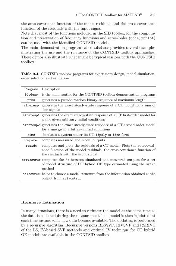
Table 9.4. CONTSID toolbox programs for experiment design, model simulation,order selection and validation
Program Description
idcdemo is the main routine for the CONTSID toolbox demonstration programs
prbs generates a pseudo-random binary sequence of maximum length
sineresp generates the exact steady-state response of a CT model for a sum ofsine signals
sineresp1 generates the exact steady-state response of a CT first-order model fora sine given arbitrary initial conditions
sineresp2 generates the exact steady-state response of a CT second-order modelfor a sine given arbitrary initial conditions
simc simulates a system under its CT idpoly or idss form
comparec compares measured and model outputs
residc computes and plots the residuals of a CT model. Plots the autocovari-ance function of the model residuals, the cross-covariance function ofthe residuals with the input signal
srivcstruc computes the fit between simulated and measured outputs for a setof model structure of CT hybrid OE type estimated using the srivc
method
selcstruc helps to choose a model structure from the information obtained as theoutput from srivcstruc
Recursive Estimation
In many situations, there is a need to estimate the model at the same time asthe data is collected during the measurement. The model is then ‘updated’ ateach time instant some new data become available. The updating is performedby a recursive algorithm. Recursive versions RLSSVF, RIVSVF and RSRIVCof the LS, IV-based SVF methods and optimal IV technique for CT hybridOE models are available in the CONTSID toolbox.
260 H. Garnier et al.
Identification from Non-uniformly Sampled Data
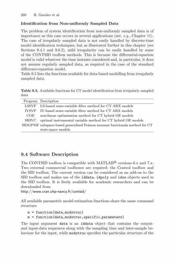
The problem of system identification from non-uniformly sampled data is ofimportance as this case occurs in several applications (see, e.g., Chapter 11).The case of irregularly sampled data is not easily handled by discrete-timemodel identification techniques, but as illustrated further in this chapter (seeSections 9.4.1 and 9.6.2), mild irregularity can be easily handled by someof the CONTSID toolbox methods. This is because the differential-equationmodel is valid whatever the time instants considered and, in particular, it doesnot assume regularly sampled data, as required in the case of the standarddifference-equation model.Table 9.5 lists the functions available for data-based modelling from irregularlysampled data.
Table 9.5. Available functions for CT model identification from irregularly sampleddata
Program Description
LSSVF LS-based state-variable filter method for CT ARX models
IVSVF IV-based state-variable filter method for CT ARX models
COE non-linear optimisation method for CT hybrid OE models
SRIVC optimal instrumental variable method for CT hybrid OE models
SIDGPMF subspace-based generalised Poisson moment functionals method for CTstate-space models
9.4 Software Description
The CONTSID toolbox is compatible with MATLAB� versions 6.x and 7.x.Two external commercial toolboxes are required: the Control toolbox andthe SID toolbox. The current version can be considered as an add-on to theSID toolbox and makes use of the iddata, idpoly and idss objects used inthe SID toolbox. It is freely available for academic researchers and can bedownloaded fromhttp://www.cran.uhp-nancy.fr/contsid/
All available parametric model estimation functions share the same commandstructure
m = function(data,modstruc)m = function(data,modstruc,specific parameters)
The input argument data is an iddata object that contains the output-and input-data sequences along with the sampling time and inter-sample be-haviour for the input, while modstruc specifies the particular structure of the
9 The CONTSID toolbox for MATLAB� 261
model to be estimated. The specific parameters depend on the preprocessingmethod used. The resulting estimated model is contained in m, which is amodel object that stores the various usual information. The function nameis defined by the abbreviation for the estimation method and the abbrevia-tion for the associated preprocessing technique, as for example, IVSVF forthe instrumental variable-based state-variable filter approach or SIDGPMFfor subspace-based state-space model identification GPMF approach.Note that help on any CONTSID toolbox function may be obtained from thecommand window by invoking classically help name function.
9.4.1 Introductory Example to the Command Mode
A part of the first demonstration program is presented in this section. Thisdemo is designed to get the new user started quickly with the CONTSIDtoolbox: it is straightforward to run the demo by typing idcdemo1 in theMATLAB� command window) and follow along. This example considers asecond-order SISO CT system without delay. The complete equation for thedata-generating system has the following form
y(tk) =3
p2 + 4p + 3u(tk) + e(tk) (9.15)
where e(tk) is a zero-mean DT white Gaussian noise sequence. Let us first cre-ate an idpoly model structure object describing the model. The polynomialsare entered in descending powers of the differential operator
m0=idpoly(1,[3],1,1,[1 4 3],’Ts’,0);
‘Ts’ and 0 indicate here that the system is time continuous.We take a PRBS of maximum length with 1016 points as input u. The sam-pling period is chosen to be 0.05 s
u = prbs(7,8);Ts = 0.05;
We then create an iddata object for the input signal with no output, the inputu and sampling interval Ts. The input inter-sample behaviour is specified bysetting the property ’Intersample’ to ’zoh’ since the input is piecewise-constant here
datau = iddata([],u,Ts,’InterSample’,’zoh’);
The noise-free output is simulated with the simc CONTSID routine and storedin ydet. We then create an iddata object with output ydet, input u andsampling interval Ts
ydet = simc(m0,datau);datadet = iddata(ydet,u,Ts,’InterSample’,’zoh’);
262 H. Garnier et al.
We then identify a CT ARX model for this system from the determinis-tic iddata object datadet with the conventional least squares-based state-variable filter (lssvf) method. The extra pieces of information required are
• the number of denominator and numerator parameters and number ofsamples for the delay of the model [na nb nk] =[2 1 0];
• the cut-off frequency (in rad/s) of the SVF filter, set to 2 here.
The lssvf routine can now be used as follows
mlssvf = lssvf(datadet,[2 1 0],2)
which leads to5
CT IDPOLY model: A(s)y(t) = B(s)u(t) + e(t)A(s) = s2 + 3.999 s + 2.999B(s) = 2.999Estimated using LSSVFLoss function 6.03708e-15 and FPE 6.07284e-15
It will be noted that, not surprisingly, the estimated model coefficients are veryclose to the true parameters. This is, of course, because the measurements arenot noise corrupted. Note that even in the noise-free case, the true parametersare not estimated exactly here. This is due to small simulation errors intro-duced in the numerical implementation of the continuous-time state-variablefiltering for the output signal.Let us now consider the case when a white Gaussian noise is added to theoutput samples. The variance of e(tk) is adjusted to obtain a signal-to-noiseratio (SNR) of 10 dB. The SNR is defined as
SNR = 10 logPydet
Pe(9.16)
where Pe represents the average power of the zero-mean additive noise on thesystem output (e.g., the variance) while Pydet
denotes the average power ofthe noise-free output fluctuations.
snr=10;y = simc(m0,datau,snr);data = iddata(y,u,Ts);
The input/output data are displayed in Figure 9.1. The use of this noisy out-put in the basic lssvf routine will inevitably lead to biased estimates. Abias-reduction algorithm based on the two-step instrumental variable tech-nique where the instruments are built up from an auxiliary model (ivsvf)can be used instead5 Note that in the Matlab� System Identification (SID) toolbox, the variable ’s’
instead of ’p’ is used to denote the differential operator. The CONTSID toolboxmakes use of the SID object models ; therefore the CONTSID estimated modelsare displayed with the ’s’ variable.
9 The CONTSID toolbox for MATLAB� 263
0 5 10 15 20 25 30 35 40 45 50−1.5
−1
−0.5
0
0.5
1
1.5O
utpu
t
0 5 10 15 20 25 30 35 40 45 50−1.5
−1
−0.5
0
0.5
1
1.5
Inpu
t
Time (s)
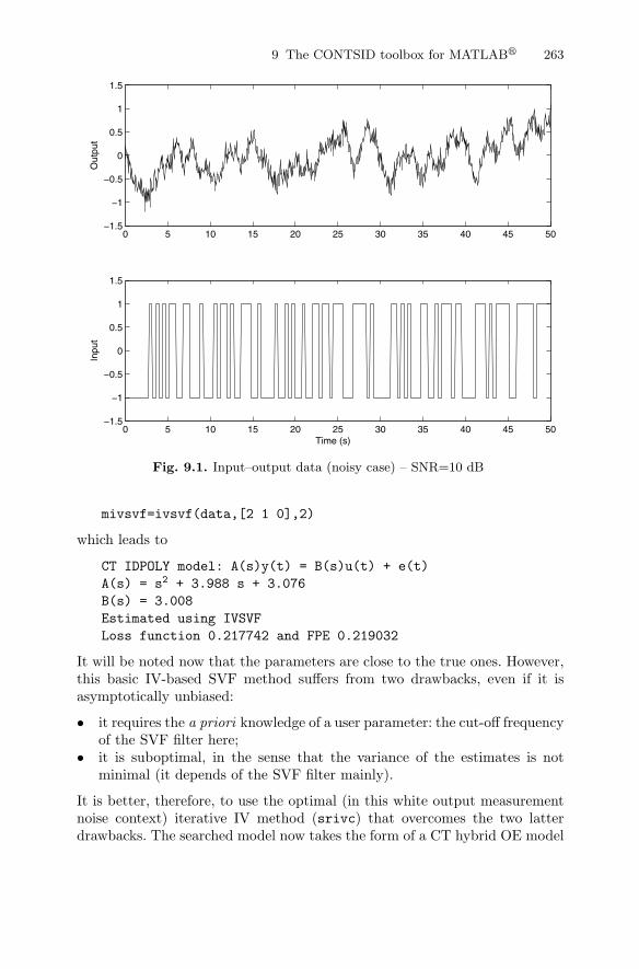
Fig. 9.1. Input–output data (noisy case) – SNR=10 dB
mivsvf=ivsvf(data,[2 1 0],2)
which leads to
CT IDPOLY model: A(s)y(t) = B(s)u(t) + e(t)A(s) = s2 + 3.988 s + 3.076B(s) = 3.008Estimated using IVSVFLoss function 0.217742 and FPE 0.219032
It will be noted now that the parameters are close to the true ones. However,this basic IV-based SVF method suffers from two drawbacks, even if it isasymptotically unbiased:
• it requires the a priori knowledge of a user parameter: the cut-off frequencyof the SVF filter here;
• it is suboptimal, in the sense that the variance of the estimates is notminimal (it depends of the SVF filter mainly).
It is better, therefore, to use the optimal (in this white output measurementnoise context) iterative IV method (srivc) that overcomes the two latterdrawbacks. The searched model now takes the form of a CT hybrid OE model
264 H. Garnier et al.
0 10 20 30 40 50−1.5
−1
−0.5
0
0.5
1
1.5
Time (s)
noisy output
simulated model output
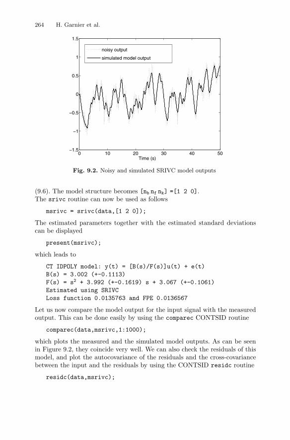
Fig. 9.2. Noisy and simulated SRIVC model outputs
(9.6). The model structure becomes [nb nf nk] =[1 2 0].The srivc routine can now be used as follows
msrivc = srivc(data,[1 2 0]);
The estimated parameters together with the estimated standard deviationscan be displayed
present(msrivc);
which leads to
CT IDPOLY model: y(t) = [B(s)/F(s)]u(t) + e(t)B(s) = 3.002 (+-0.1113)F(s) = s2 + 3.992 (+-0.1619) s + 3.067 (+-0.1061)Estimated using SRIVCLoss function 0.0135763 and FPE 0.0136567
Let us now compare the model output for the input signal with the measuredoutput. This can be done easily by using the comparec CONTSID routine
comparec(data,msrivc,1:1000);
which plots the measured and the simulated model outputs. As can be seenin Figure 9.2, they coincide very well. We can also check the residuals of thismodel, and plot the autocovariance of the residuals and the cross-covariancebetween the input and the residuals by using the CONTSID residc routine
residc(data,msrivc);
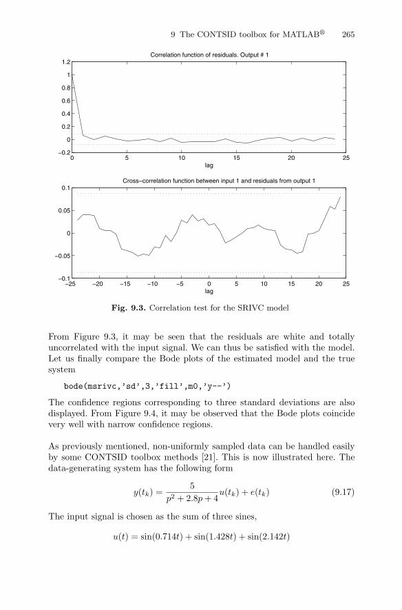
9 The CONTSID toolbox for MATLAB� 265
0 5 10 15 20 25−0.2
0
0.2
0.4
0.6
0.8
1
1.2Correlation function of residuals. Output # 1
lag
−25 −20 −15 −10 −5 0 5 10 15 20 25−0.1
−0.05
0
0.05
0.1Cross−correlation function between input 1 and residuals from output 1
lag
Fig. 9.3. Correlation test for the SRIVC model
From Figure 9.3, it may be seen that the residuals are white and totallyuncorrelated with the input signal. We can thus be satisfied with the model.Let us finally compare the Bode plots of the estimated model and the truesystem
bode(msrivc,’sd’,3,’fill’,m0,’y--’)
The confidence regions corresponding to three standard deviations are alsodisplayed. From Figure 9.4, it may be observed that the Bode plots coincidevery well with narrow confidence regions.
As previously mentioned, non-uniformly sampled data can be handled easilyby some CONTSID toolbox methods [21]. This is now illustrated here. Thedata-generating system has the following form
y(tk) =5
p2 + 2.8p + 4u(tk) + e(tk) (9.17)
The input signal is chosen as the sum of three sines,
u(t) = sin(0.714t) + sin(1.428t) + sin(2.142t)
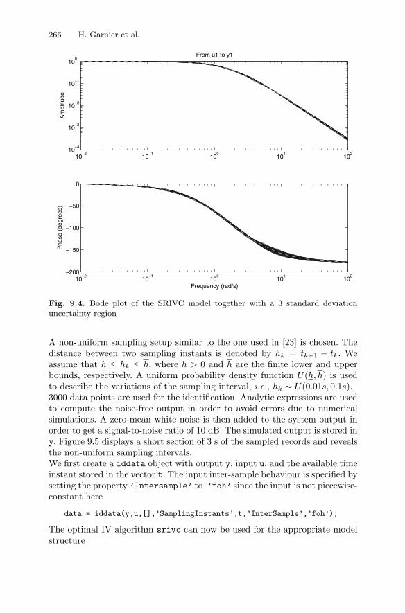
266 H. Garnier et al.
10−2
10−1
100
101
102
10−4
10−3
10−2
10−1
100
Am
plitu
deFrom u1 to y1
10−2
10−1
100
101
102
−200
−150
−100
−50
0
Pha
se (
degr
ees)
Frequency (rad/s)
Fig. 9.4. Bode plot of the SRIVC model together with a 3 standard deviationuncertainty region
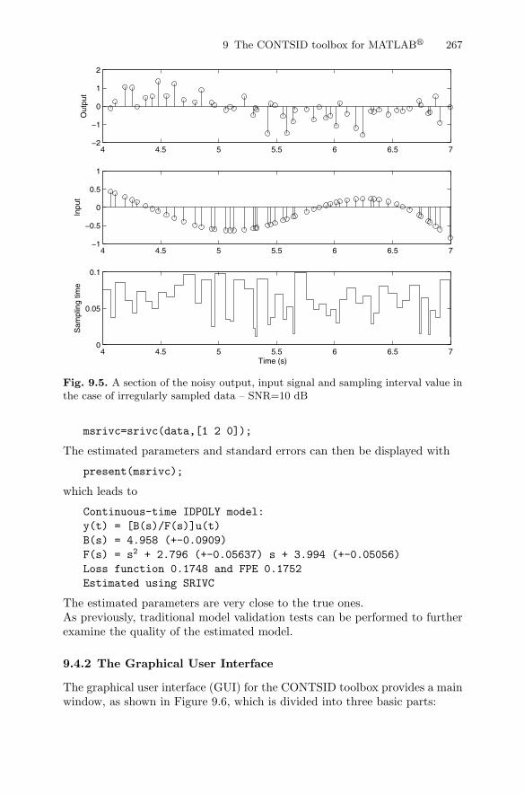
A non-uniform sampling setup similar to the one used in [23] is chosen. Thedistance between two sampling instants is denoted by hk = tk+1 − tk. Weassume that h ≤ hk ≤ h, where h > 0 and h are the finite lower and upperbounds, respectively. A uniform probability density function U(h, h) is usedto describe the variations of the sampling interval, i.e., hk ∼ U(0.01s, 0.1s).3000 data points are used for the identification. Analytic expressions are usedto compute the noise-free output in order to avoid errors due to numericalsimulations. A zero-mean white noise is then added to the system output inorder to get a signal-to-noise ratio of 10 dB. The simulated output is stored iny. Figure 9.5 displays a short section of 3 s of the sampled records and revealsthe non-uniform sampling intervals.We first create a iddata object with output y, input u, and the available timeinstant stored in the vector t. The input inter-sample behaviour is specified bysetting the property ’Intersample’ to ’foh’ since the input is not piecewise-constant here
data = iddata(y,u,[],’SamplingInstants’,t,’InterSample’,’foh’);
The optimal IV algorithm srivc can now be used for the appropriate modelstructure
9 The CONTSID toolbox for MATLAB� 267
4 4.5 5 5.5 6 6.5 7−2
−1
0
1
2
Out
put
4 4.5 5 5.5 6 6.5 7−1
−0.5
0
0.5
1
Inpu
t
4 4.5 5 5.5 6 6.5 70
0.05
0.1
Sam
plin
g tim
e
Time (s)
Fig. 9.5. A section of the noisy output, input signal and sampling interval value inthe case of irregularly sampled data – SNR=10 dB
msrivc=srivc(data,[1 2 0]);
The estimated parameters and standard errors can then be displayed with
present(msrivc);
which leads to
Continuous-time IDPOLY model:y(t) = [B(s)/F(s)]u(t)B(s) = 4.958 (+-0.0909)F(s) = s2 + 2.796 (+-0.05637) s + 3.994 (+-0.05056)Loss function 0.1748 and FPE 0.1752Estimated using SRIVC
The estimated parameters are very close to the true ones.As previously, traditional model validation tests can be performed to furtherexamine the quality of the estimated model.
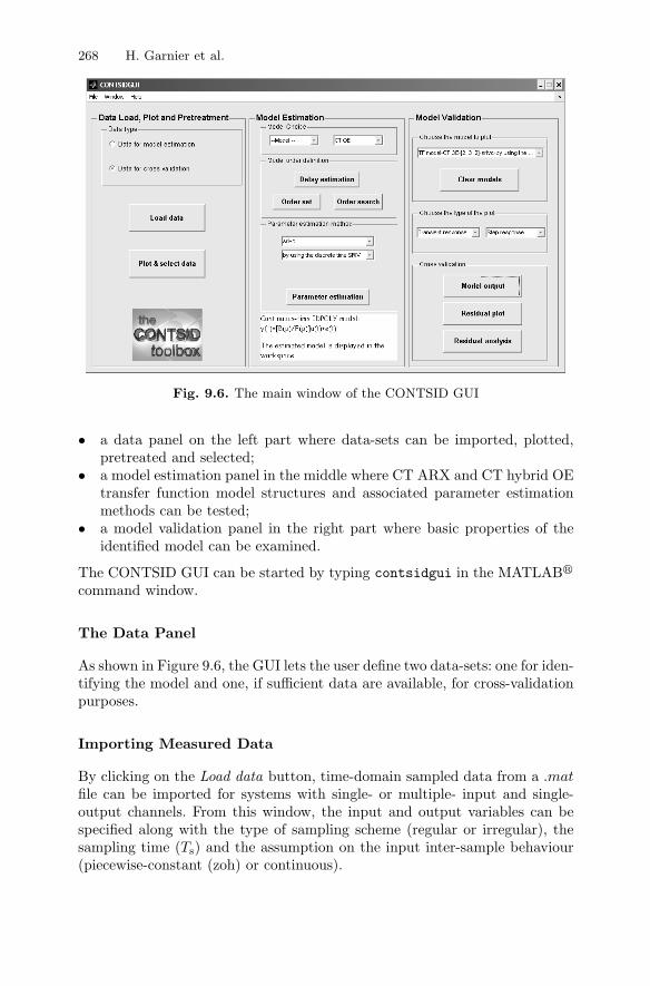
9.4.2 The Graphical User Interface
The graphical user interface (GUI) for the CONTSID toolbox provides a mainwindow, as shown in Figure 9.6, which is divided into three basic parts:
268 H. Garnier et al.
Fig. 9.6. The main window of the CONTSID GUI
• a data panel on the left part where data-sets can be imported, plotted,pretreated and selected;
• a model estimation panel in the middle where CT ARX and CT hybrid OEtransfer function model structures and associated parameter estimationmethods can be tested;
• a model validation panel in the right part where basic properties of theidentified model can be examined.
The CONTSID GUI can be started by typing contsidgui in the MATLAB�
command window.
The Data Panel
As shown in Figure 9.6, the GUI lets the user define two data-sets: one for iden-tifying the model and one, if sufficient data are available, for cross-validationpurposes.
Importing Measured Data
By clicking on the Load data button, time-domain sampled data from a .matfile can be imported for systems with single- or multiple- input and single-output channels. From this window, the input and output variables can bespecified along with the type of sampling scheme (regular or irregular), thesampling time (Ts) and the assumption on the input inter-sample behaviour(piecewise-constant (zoh) or continuous).
9 The CONTSID toolbox for MATLAB� 269
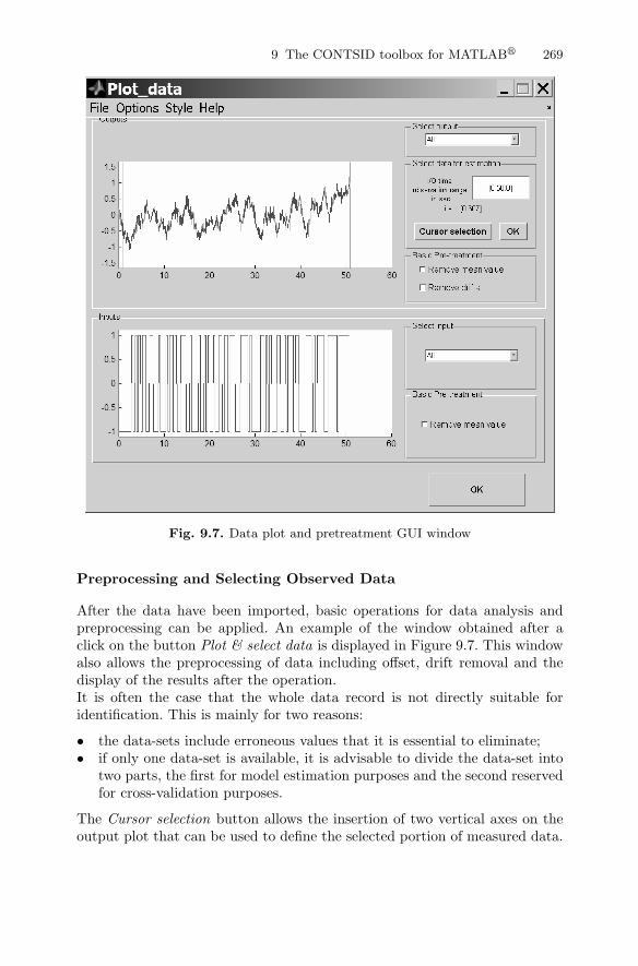
Fig. 9.7. Data plot and pretreatment GUI window
Preprocessing and Selecting Observed Data
After the data have been imported, basic operations for data analysis andpreprocessing can be applied. An example of the window obtained after aclick on the button Plot & select data is displayed in Figure 9.7. This windowalso allows the preprocessing of data including offset, drift removal and thedisplay of the results after the operation.It is often the case that the whole data record is not directly suitable foridentification. This is mainly for two reasons:
• the data-sets include erroneous values that it is essential to eliminate;• if only one data-set is available, it is advisable to divide the data-set into
two parts, the first for model estimation purposes and the second reservedfor cross-validation purposes.
The Cursor selection button allows the insertion of two vertical axes on theoutput plot that can be used to define the selected portion of measured data.
270 H. Garnier et al.
Model Estimation Panel
While the CONTSID toolbox supports transfer function and state-spacemodel identification methods, the GUI lets the user estimate CT ARX andhybrid OE models only. The user is thus invited to choose the type of modelstructure in the unrolling menu at the top right of the model estimation panel,as shown in Figure 9.6.After selecting the model structure, the user has to specify the polynomialorders and the time delay of the model to be estimated.A first option is to deduce an estimate of the number of samples for the timedelay from an estimation of the impulse response by correlation analysis.Then, if the TF model orders are not known a priori, the Order search buttonallows the user to automatically search over a whole range of different modelorders. The user can choose several available criteria to sort and display theestimation results in the MATLAB� workspace. From these results, the usercan select the best model orders and then set the order of the final model tobe estimated by clicking on the Order set button from the main window.Once the number of samples for the time delay and the number of coefficientsfor the polynomial model have been set, the model parameters can then beestimated by using one of the available parametric estimation methods chosenfrom an unrolling menu
• in the case of a CT hybrid OE model structure, the user can choose to usethe continuous-time output error (COE) method or the simplified refinedinstrumental variable (SRIVC) method;
• in the case of a CT ARX model structure, the user can select one ofthe six preprocessing-based methods that have proven successful. Thesepreprocessing methods are coupled with conventional least squares or basicauxiliary model-based instrumental variable methods. These all require auser parameter to be specified by the user [17] which should be chosen inorder to emphasise the frequency band of interest.
Once the parameter estimation method is chosen, the identified model is dis-played in the command window after a click on the Parameter estimationbutton.
Model Validation Panel
Once a model is estimated, it appears in the drop-down menu located at thetop part of the Model Validation panel (see Figure 9.6). Several basic modelproperties can then be evaluated from an unrolling menu by using first thedata that were used for model identification
• model-output comparison: plots and compares the simulated model outputwith the measured output. This indicates how well the system dynamicsare captured;
9 The CONTSID toolbox for MATLAB� 271
• residual plot : displays the residuals;• transient response: displays the model response to an impulse or step ex-
citation signal;• frequency response: displays the Nyquist or Bode plots to show damping
levels and resonance frequencies;• zeros and poles : plots the zeros and poles of the identified models and tests
for zero-pole cancelation indicating overparameterised modelling;• correlation test : displays the autocovariance function of the residuals and
the cross-covariance function between the input signal and the residuals.
If a cross-validation data-set is available, then traditional cross-validation testsconsist of comparisons between the measured and simulated model outputsand analysis of the residuals.
9.5 Advantages and Relevance of the CONTSID ToolboxMethods
There are two fundamentally different time-domain approaches to the prob-lem of obtaining a CT model of a naturally CT system from its sampledinput/output data:
• the indirect approach that involves two steps. First, a DT model for theoriginal CT system is obtained by applying the DT model estimation meth-ods and the DT model is then transformed into CT form;
• the direct approach where a CT model is obtained straightaway using CTmodel identification methods discussed in this chapter.
The indirect approach has the advantage that it uses well-established DTmodel identification methods [24, 41]. Examples of such methods, which areknown to give consistent and statistically efficient estimates under very gen-eral conditions, are gradient-optimisation procedures, such as the maximumlikelihood and prediction error methods in the SID toolbox; and iterative, re-laxation procedures, such as the refined instrumental variable (RIV) methodin the CAPTAIN toolbox.On the surface, the choice between the two approaches may seem trivial.However, some recent studies have shown some serious shortcomings of theindirect route through DT models. Indeed, an extensive analysis aimed atcomparing direct and indirect approaches has been discussed recently. Thesimulation model used in this analysis provides a very good test for CT andDT model estimation methods: it was first suggested by Rao and Garnier [36](see also [17,37,38]); further investigations by Ljung [25] confirmed the results.This example illustrates some of the well-known difficulties that may appearin DT modelling under less standard conditions such as rapidly sampled dataor relatively wide-band systems:
272 H. Garnier et al.
• relatively high sensitivity to the initialisation. DT model identification of-ten requires computationally costly minimisation algorithms without evenguaranteeing convergence (to the global optimum). In fact, in many cases,the initialisation procedure for the identification scheme is a key factorto obtain satisfactory estimation results compared to direct methods (see,e.g., [50] for a recent reference);
• numerical issues in the case of fast sampling because the eigenvalues lieclose to the unit circle in the complex domain, so that the model param-eters are more poorly defined in statistical terms;
• a priori knowledge of the relative degree is not easy to accommodate;• non-inherent data prefiltering in the gradient-based methods (adaptive
prefiltering is an inherent part of the DT RIV method in CAPTAIN).
Further, the question of parameter transformation between a DT descriptionand a CT representation is non-trivial. First, the zeros of the DT model arenot as easily translatable to CT equivalents as the poles [2]; second, due to thediscrete nature of the measurements they do not contain all the informationabout the CT signals. To describe the signals between the sampling instantssome additional assumptions have to be made, for example, assuming that theexcitation signal is constant between the sampling intervals (zero-order holdassumption). Violation of these assumptions may lead to severe estimationerrors [40].The advantages of direct CT identification approaches over the alternativeDT identification methods can be summarised as follows:
• they directly provide differential-equation models whose parameters canbe interpreted immediately in physically meaningful terms. As a result,they are of direct use to scientists and engineers who most often derivemodels in differential-equation terms based on natural laws and who aremuch less familiar with ‘black-box’ discrete-time models;
• they can estimate a fractional time-delay system;• the estimated model is defined by a unique set of parameter values that
are not dependent on the sampling interval Ts;• there is no need for conversion from discrete to continuous time, as required
in the indirect route based on initial DT model estimation;• the direct continuous-time methods can easily handle the case of mild
irregularity in the sampled data;• the a priori knowledge of the relative degree is easy to accommodate and
therefore allows the identification of more parsimonious models than indiscrete time;
• they also offer advantages when applied to systems with widely separatedmodes;
• they include inherent data filtering;• they are well suited in the case of very rapid sampling. This is particularly
interesting since modern data-acquisition equipment can provide nearlycontinuous-time measurements and, therefore, make it possible to acquire
9 The CONTSID toolbox for MATLAB� 273
data at very high sampling frequencies. Note that, as mentioned in [25], theuse of prefiltering and decimation strategies may lead to better results inthe case of DT modelling, but these may not be so obvious for practitioners.The CONTSID toolbox methods are free of these difficulties.
All these advantages will facilitate for the user the application of the gen-eral data-based modelling procedure. In the following, these advantages areillustrated with the help of a simulated benchmark system.
The SYSID’2006 Benchmark System
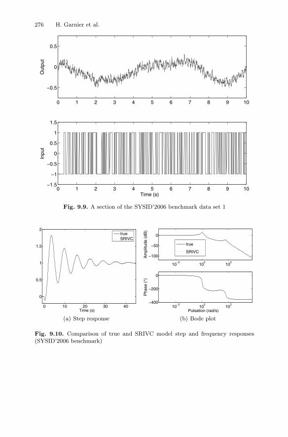
Here, the performance of the CONTSID toolbox techniques is illustrated byapplying them to a benchmark example that was prepared for the 14th IFACSymposium on System Identification (SYSID’06) in Newcastle, Australia6.The intent of the benchmark was to set up a format in which rigorous com-parisons between competing techniques for the identification of CT modelsfrom sampled data, including time- and frequency-domain approaches, couldbe undertaken. The goal was also to collect and analyse quantitative resultsin order to understand similarities and differences among the approaches andto highlight the strengths and weaknesses of each approach.Two benchmark data sets were generated. Both were simulated continuous-time systems based closely on mechatronic systems. Data corresponding tothese two benchmarks were sent to participants to apply their preferred tech-nique.Unfortunately, the associated Benchmark Session at SYSID was cancelledbecause referees felt that insufficient submitted papers were acceptable (onlyone of the papers submitted to the proposed benchmark session got evenclose to the correct model, demonstrating the difficulty of the benchmarkexercise). This section presents the CONTSID toolbox results obtained on thebenchmark data set 1, in which the additive measurement noise is a simplewhite additive noise. The second benchmark data set is more difficult since thewhite measurement noise is replaced by non-stationary noise (similar resultswere obtained using the CAPTAIN toolbox routines [50], where a modifiedexample with coloured additive noise is considered).The SYSID Benchmark data set 1 is obtained from
{x(t) = Go(p)u(t), subject to zero initial conditionsy(tk) = x(tk) + e(tk)
(9.18)
where the measurement noise e(tk) is a zero-mean DT white Gaussian se-quence.The system is a linear, fourth-order, non-minimum phase system with complexpoles where the Laplace transfer function is given by6 The data can be downloaded fromhttp://sysid2006benchmark.cran.uhp-nancy.fr/.
274 H. Garnier et al.
0 10 20 30 40
0
0.5
1
1.5
2
Time (s)
(a) Step response
10−2
100
102
−100
−50
0
Am
plitu
de (
dB)
10−2
100
102
−400
−200
0
Pha
se (
°)
Pulsation (rad/s)
(b) Bode plot
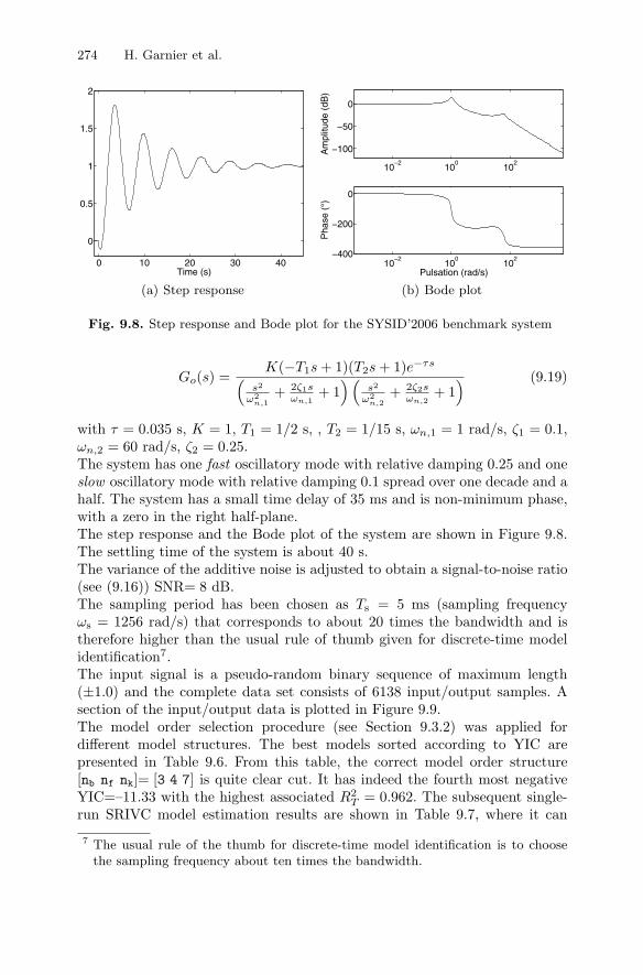
Fig. 9.8. Step response and Bode plot for the SYSID’2006 benchmark system
Go(s) =K(−T1s + 1)(T2s + 1)e−τs(
s2
ω2n,1
+ 2ζ1sωn,1
+ 1)(
s2
ω2n,2
+ 2ζ2sωn,2
+ 1) (9.19)
with τ = 0.035 s, K = 1, T1 = 1/2 s, , T2 = 1/15 s, ωn,1 = 1 rad/s, ζ1 = 0.1,ωn,2 = 60 rad/s, ζ2 = 0.25.The system has one fast oscillatory mode with relative damping 0.25 and oneslow oscillatory mode with relative damping 0.1 spread over one decade and ahalf. The system has a small time delay of 35 ms and is non-minimum phase,with a zero in the right half-plane.The step response and the Bode plot of the system are shown in Figure 9.8.The settling time of the system is about 40 s.The variance of the additive noise is adjusted to obtain a signal-to-noise ratio(see (9.16)) SNR= 8 dB.The sampling period has been chosen as Ts = 5 ms (sampling frequencyωs = 1256 rad/s) that corresponds to about 20 times the bandwidth and istherefore higher than the usual rule of thumb given for discrete-time modelidentification7.The input signal is a pseudo-random binary sequence of maximum length(±1.0) and the complete data set consists of 6138 input/output samples. Asection of the input/output data is plotted in Figure 9.9.The model order selection procedure (see Section 9.3.2) was applied fordifferent model structures. The best models sorted according to YIC arepresented in Table 9.6. From this table, the correct model order structure[nb nf nk]= [3 4 7] is quite clear cut. It has indeed the fourth most negativeYIC=–11.33 with the highest associated R2
T = 0.962. The subsequent single-run SRIVC model estimation results are shown in Table 9.7, where it can
7 The usual rule of the thumb for discrete-time model identification is to choosethe sampling frequency about ten times the bandwidth.
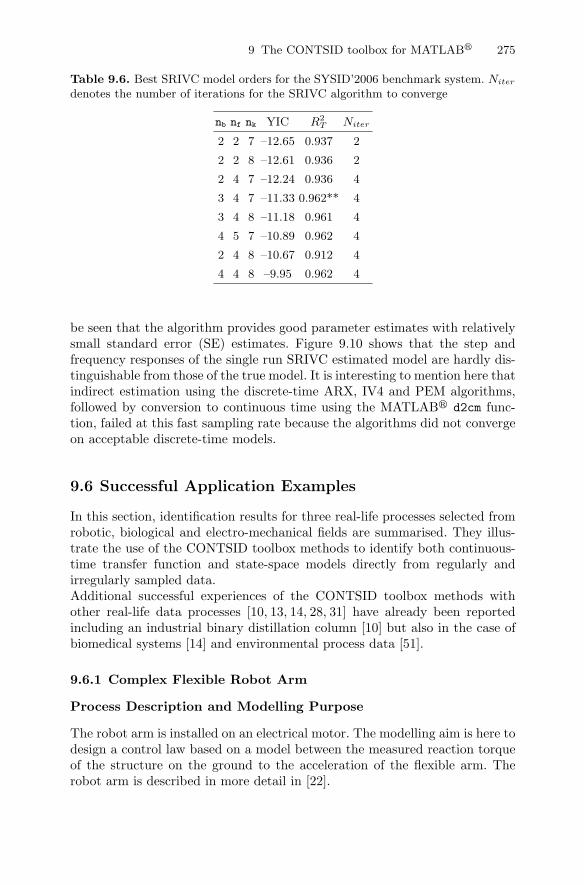
9 The CONTSID toolbox for MATLAB� 275
Table 9.6. Best SRIVC model orders for the SYSID’2006 benchmark system. Niter
denotes the number of iterations for the SRIVC algorithm to converge
nb nf nk YIC R2T Niter
2 2 7 –12.65 0.937 2
2 2 8 –12.61 0.936 2
2 4 7 –12.24 0.936 4
3 4 7 –11.33 0.962** 4
3 4 8 –11.18 0.961 4
4 5 7 –10.89 0.962 4
2 4 8 –10.67 0.912 4
4 4 8 –9.95 0.962 4
be seen that the algorithm provides good parameter estimates with relativelysmall standard error (SE) estimates. Figure 9.10 shows that the step andfrequency responses of the single run SRIVC estimated model are hardly dis-tinguishable from those of the true model. It is interesting to mention here thatindirect estimation using the discrete-time ARX, IV4 and PEM algorithms,followed by conversion to continuous time using the MATLAB� d2cm func-tion, failed at this fast sampling rate because the algorithms did not convergeon acceptable discrete-time models.
9.6 Successful Application Examples
In this section, identification results for three real-life processes selected fromrobotic, biological and electro-mechanical fields are summarised. They illus-trate the use of the CONTSID toolbox methods to identify both continuous-time transfer function and state-space models directly from regularly andirregularly sampled data.Additional successful experiences of the CONTSID toolbox methods withother real-life data processes [10, 13, 14, 28, 31] have already been reportedincluding an industrial binary distillation column [10] but also in the case ofbiomedical systems [14] and environmental process data [51].
9.6.1 Complex Flexible Robot Arm
Process Description and Modelling Purpose
The robot arm is installed on an electrical motor. The modelling aim is here todesign a control law based on a model between the measured reaction torqueof the structure on the ground to the acceleration of the flexible arm. Therobot arm is described in more detail in [22].
276 H. Garnier et al.
0 1 2 3 4 5 6 7 8 9 10
−0.5
0
0.5O
utpu
t
0 1 2 3 4 5 6 7 8 9 10−1.5
−1
−0.5
0
0.5
1
1.5
Inpu
t
Time (s)
Fig. 9.9. A section of the SYSID’2006 benchmark data set 1
0 10 20 30 40
0
0.5
1
1.5
2
Time (s)
trueSRIVC
(a) Step response
10−2
100
102
−100
−50
0
Am
plitu
de (
dB)
10−2
100
102
−400
−200
0
Pulsation (rad/s)
Pha
se (
°)
true
SRIVC
(b) Bode plot
Fig. 9.10. Comparison of true and SRIVC model step and frequency responses(SYSID’2006 benchmark)
9 The CONTSID toolbox for MATLAB� 277
Table 9.7. SYSID’2006 benchmark system estimation results
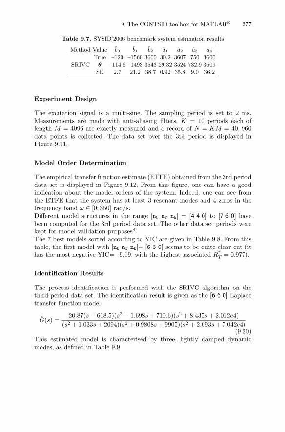
Method Value b0 b1 b2 a1 a2 a3 a4
True –120 –1560 3600 30.2 3607 750 3600
SRIVC θ –114.6 –1493 3543 29.32 3524 732.9 3509SE 2.7 21.2 38.7 0.92 35.8 9.0 36.2
Experiment Design
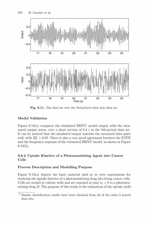
The excitation signal is a multi-sine. The sampling period is set to 2 ms.Measurements are made with anti-aliasing filters. K = 10 periods each oflength M = 4096 are exactly measured and a record of N = KM = 40, 960data points is collected. The data set over the 3rd period is displayed inFigure 9.11.
Model Order Determination
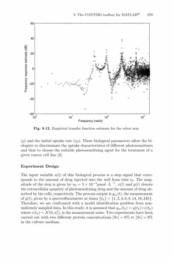
The empirical transfer function estimate (ETFE) obtained from the 3rd perioddata set is displayed in Figure 9.12. From this figure, one can have a goodindication about the model orders of the system. Indeed, one can see fromthe ETFE that the system has at least 3 resonant modes and 4 zeros in thefrequency band ω ∈ [0; 350] rad/s.Different model structures in the range [nb nf nk] = [4 4 0] to [7 6 0] havebeen computed for the 3rd period data set. The other data set periods werekept for model validation purposes8.The 7 best models sorted according to YIC are given in Table 9.8. From thistable, the first model with [nb nf nk]= [6 6 0] seems to be quite clear cut (ithas the most negative YIC=−9.19, with the highest associated R2
T = 0.977).
Identification Results
The process identification is performed with the SRIVC algorithm on thethird-period data set. The identification result is given as the [6 6 0] Laplacetransfer function model
G(s) =20.87(s − 618.5)(s2 − 1.698s + 710.6)(s2 + 8.435s + 2.012e4)
(s2 + 1.033s + 2094)(s2 + 0.9808s + 9905)(s2 + 2.693s + 7.042e4)(9.20)
This estimated model is characterised by three, lightly damped dynamicmodes, as defined in Table 9.9.
278 H. Garnier et al.
17 18 19 20 21 22 23 24
−0.5
0
0.5
Out
put
17 18 19 20 21 22 23 24−0.4
−0.2
0
0.2
0.4
Inpu
t
Time (s)
Fig. 9.11. The data set over the 3rd-period robot arm data set
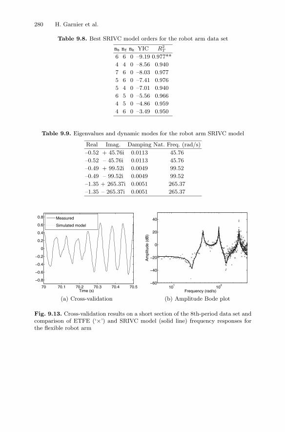
Model Validation
Figure 9.13(a) compares the simulated SRIVC model output with the mea-sured output series, over a short section of 0.4 s in the 8th-period data set.It can be noticed that the simulated output matches the measured data quitewell, with R2
T > 0.95. There is also a very good agreement between the ETFEand the frequency response of the estimated SRIVC model, as shown in Figure9.13(b).
9.6.2 Uptake Kinetics of a Photosensitising Agent into CancerCells
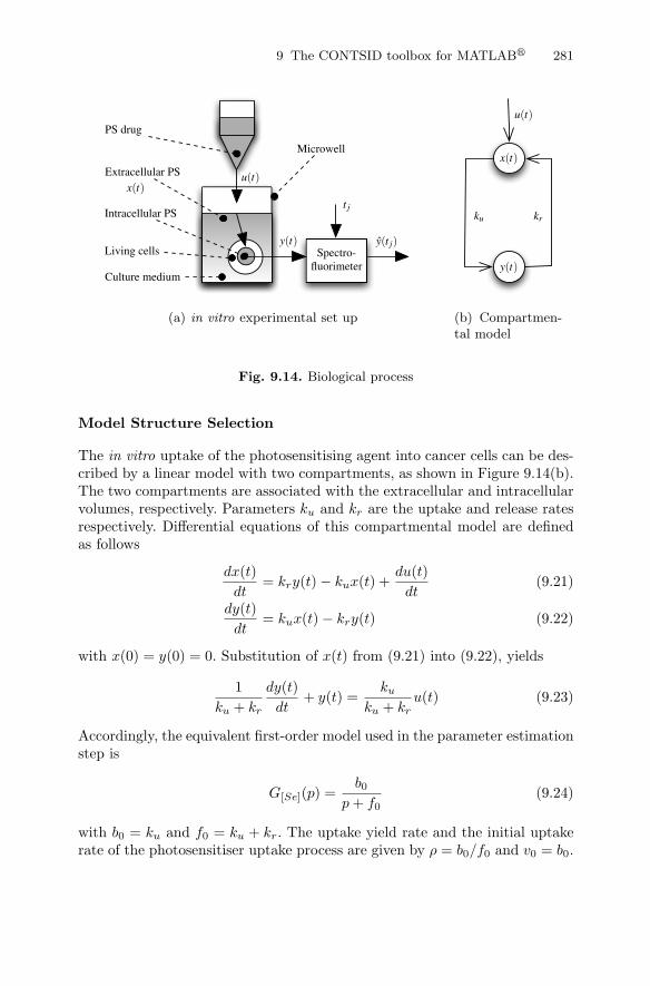
Process Description and Modelling Purpose
Figure 9.14(a) depicts the basic material used in in vitro experiments forstudying the uptake kinetics of a photosensitising drug into living cancer cells.Cells are seeded in culture wells and are exposed at time t0 = 0 to a photosen-sitising drug D. The purpose of this study is the estimation of the uptake yield
8 Similar identification results have been obtained from all of the other 9 perioddata sets.
9 The CONTSID toolbox for MATLAB� 279
100
101
102
103
−60
−40
−20
0
20
40
60
Frequency (rad/s)
Fre
quen
cy r
espo
nse
estim
ate
(dB
)
Fig. 9.12. Empirical transfer function estimate for the robot arm
(ρ) and the initial uptake rate (v0). These biological parameters allow the bi-ologists to discriminate the uptake characteristics of different photosensitisersand thus to choose the suitable photosensitising agent for the treatment of agiven cancer cell line [3].
Experiment Design
The input variable u(t) of this biological process is a step signal that corre-sponds to the amount of drug injected into the well from time t0. The mag-nitude of the step is given by u0 = 5 × 10⁻³μmol · L−1. x(t) and y(t) denotethe extracellular quantity of photosensitising drug and the amount of drug ab-sorbed by the cells, respectively. The process output is ym(t), the measurementof y(t), given by a spectrofluorimeter at times {tk} = {1, 2, 4, 6, 8, 14, 18, 24h}.Therefore, we are confronted with a model identification problem from non-uniformly sampled data. In this study, it is assumed that ym(tk) = y(tk)+e(tk)where e(tk) ∼ N (0, σ2
e), is the measurement noise. Two experiments have beencarried out with two different protein concentrations [Se] = 0% et [Se] = 9%in the culture medium.
280 H. Garnier et al.
Table 9.8. Best SRIVC model orders for the robot arm data set
nb nf nk YIC R2T
6 6 0 –9.19 0.977**
4 4 0 –8.56 0.940
7 6 0 –8.03 0.977
5 6 0 –7.41 0.976
5 4 0 –7.01 0.940
6 5 0 –5.56 0.966
4 5 0 –4.86 0.959
4 6 0 –3.49 0.950
Table 9.9. Eigenvalues and dynamic modes for the robot arm SRIVC model
Real Imag. Damping Nat. Freq. (rad/s)
–0.52 + 45.76i 0.0113 45.76
–0.52 – 45.76i 0.0113 45.76
–0.49 + 99.52i 0.0049 99.52
–0.49 – 99.52i 0.0049 99.52
–1.35 + 265.37i 0.0051 265.37
–1.35 – 265.37i 0.0051 265.37
70 70.1 70.2 70.3 70.4 70.5
−0.8
−0.6
−0.4
−0.2
0
0.2
0.4
0.6
0.8
Time (s)
Measured
Simulated model
(a) Cross-validation
101
102
−60
−40
−20
0
20
40
Frequency (rad/s)
Am
plitu
de (
dB)
(b) Amplitude Bode plot
Fig. 9.13. Cross-validation results on a short section of the 8th-period data set andcomparison of ETFE (‘×’) and SRIVC model (solid line) frequency responses forthe flexible robot arm
9 The CONTSID toolbox for MATLAB� 281
PS drug
Extracellular PS
Culture medium
Intracellular PS
Living cells
Microwell
Spectro-fluorimeter
x(t)u(t)
y(t) y(t j)
t j
(a) in vitro experimental set up
u(t)
y(t)
x(t)
krku
(b) Compartmen-tal model
Fig. 9.14. Biological process
Model Structure Selection
The in vitro uptake of the photosensitising agent into cancer cells can be des-cribed by a linear model with two compartments, as shown in Figure 9.14(b).The two compartments are associated with the extracellular and intracellularvolumes, respectively. Parameters ku and kr are the uptake and release ratesrespectively. Differential equations of this compartmental model are definedas follows
dx(t)dt
= kry(t) − kux(t) +du(t)dt
(9.21)
dy(t)dt
= kux(t) − kry(t) (9.22)
with x(0) = y(0) = 0. Substitution of x(t) from (9.21) into (9.22), yields
1ku + kr
dy(t)dt
+ y(t) =ku
ku + kru(t) (9.23)
Accordingly, the equivalent first-order model used in the parameter estimationstep is
G[Se](p) =b0
p + f0(9.24)
with b0 = ku and f0 = ku + kr. The uptake yield rate and the initial uptakerate of the photosensitiser uptake process are given by ρ = b0/f0 and v0 = b0.
282 H. Garnier et al.
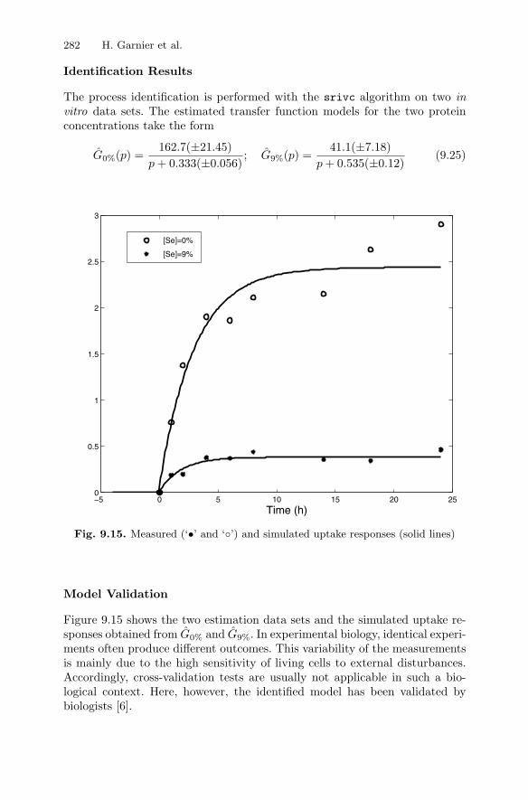
Identification Results
The process identification is performed with the srivc algorithm on two invitro data sets. The estimated transfer function models for the two proteinconcentrations take the form
G0%(p) =162.7(±21.45)
p + 0.333(±0.056); G9%(p) =
41.1(±7.18)p + 0.535(±0.12)
(9.25)
−5 0 5 10 15 20 250
0.5
1
1.5
2
2.5
3
Time (h)
[Se]=0%
[Se]=9%
Fig. 9.15. Measured (‘•’ and ‘◦’) and simulated uptake responses (solid lines)
Model Validation
Figure 9.15 shows the two estimation data sets and the simulated uptake re-sponses obtained from G0% and G9%. In experimental biology, identical experi-ments often produce different outcomes. This variability of the measurementsis mainly due to the high sensitivity of living cells to external disturbances.Accordingly, cross-validation tests are usually not applicable in such a bio-logical context. Here, however, the identified model has been validated bybiologists [6].
9 The CONTSID toolbox for MATLAB� 283
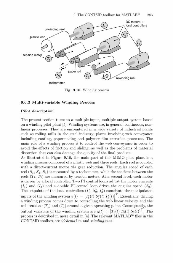
rewinding reel
unwinding reel
pacer roll
T1
T3
I3*
I1*
S2*
S2
DC motors +local controllers
tension meter
tachometer
plastic web
Fig. 9.16. Winding process
9.6.3 Multi-variable Winding Process
Pilot description
The present section turns to a multiple-input, multiple-output system basedon a winding pilot plant [5]. Winding systems are, in general, continuous, non-linear processes. They are encountered in a wide variety of industrial plantssuch as rolling mills in the steel industry, plants involving web conveyanceincluding coating, papermaking and polymer film extrusion processes. Themain role of a winding process is to control the web conveyance in order toavoid the effects of friction and sliding, as well as the problems of materialdistortion that can also damage the quality of the final product.As illustrated in Figure 9.16, the main part of this MIMO pilot plant is awinding process composed of a plastic web and three reels. Each reel is coupledwith a direct-current motor via gear reduction. The angular speed of eachreel (S1, S2, S3) is measured by a tachometer, while the tensions between thereels (T1, T3) are measured by tension meters. At a second level, each motoris driven by a local controller. Two PI control loops adjust the motor currents(I1) and (I3) and a double PI control loop drives the angular speed (S2).The setpoints of the local controllers (I∗1 , S∗
2 , I∗3 ) constitute the manipulatedinputs of the winding system u(t) =
[I∗1 (t) S∗
2 (t) I∗3 (t)]T . Essentially, driving
a winding process comes down to controlling the web linear velocity and theweb tensions (T1) and (T3) around a given operating point. Consequently, theoutput variables of the winding system are y(t) =
[T1(t) T3(t) S2(t)
]T . Theprocess is described in more detail in [4]. The relevant MATLAB� files in theCONTSID toolbox are idcdemo7.m and winding.mat.
284 H. Garnier et al.
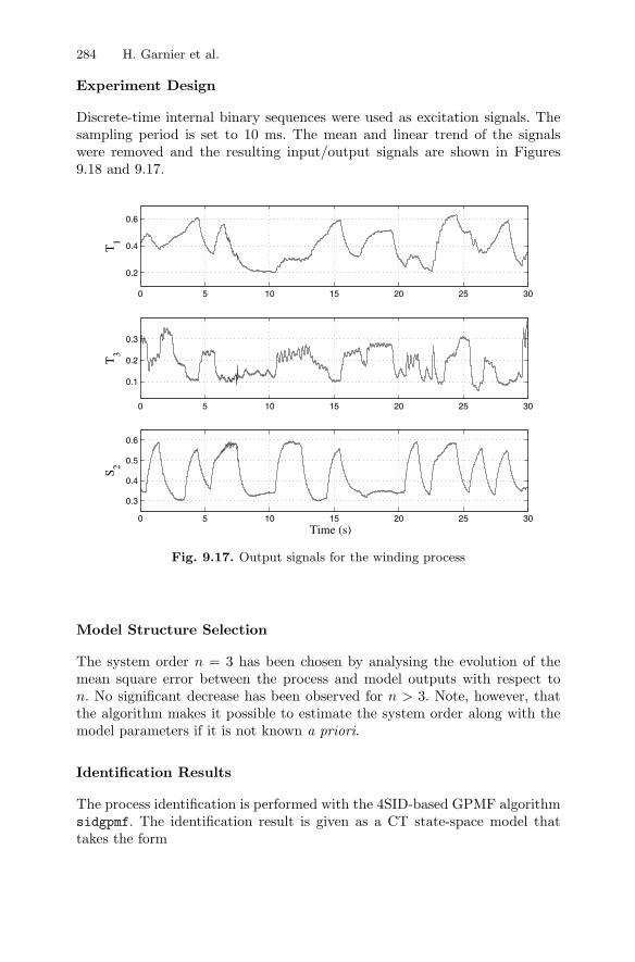
Experiment Design
Discrete-time internal binary sequences were used as excitation signals. Thesampling period is set to 10 ms. The mean and linear trend of the signalswere removed and the resulting input/output signals are shown in Figures9.18 and 9.17.
0 5 10 15 20 25 30
0.2
0.4
0.6
T1
0 5 10 15 20 25 30
0.3
0.4
0.5
0.6
S 2
Time (s)
0 5 10 15 20 25 30
0.1
0.2
0.3
T3
Fig. 9.17. Output signals for the winding process
Model Structure Selection
The system order n = 3 has been chosen by analysing the evolution of themean square error between the process and model outputs with respect ton. No significant decrease has been observed for n > 3. Note, however, thatthe algorithm makes it possible to estimate the system order along with themodel parameters if it is not known a priori.
Identification Results
The process identification is performed with the 4SID-based GPMF algorithmsidgpmf. The identification result is given as a CT state-space model thattakes the form
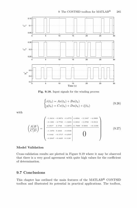
9 The CONTSID toolbox for MATLAB� 285
0 5 10 15 20 25 30
0.05
0.1
0.15
I 1*
0 5 10 15 20 25 300.3
0.4
0.5
S 2*
Time (s)
0 5 10 15 20 25 30
0.25
0.3
0.35
I 3*
Fig. 9.18. Input signals for the winding process
{x(tk) = Ax(tk) + Bu(tk)y(tk) = Cx(tk) + Du(tk) + ξ(tk)
(9.26)
with
(A BC D
)=
⎛
⎜⎜⎜⎜⎜⎜⎜⎝
−1.6414 −0.9874 −0.4773
−0.1261 −2.7725 −1.3205
0.4517 2.1746 −4.2674
4.4994 −3.1047 −4.0889
2.0652 −3.3796 −9.0513
11.7889 9.6855 −15.4186
−1.1073 0.4345 −0.0536
0.1442 −0.1717 −0.2537
−0.2047 −0.4425 0.1120
0
⎞
⎟⎟⎟⎟⎟⎟⎟⎠
(9.27)
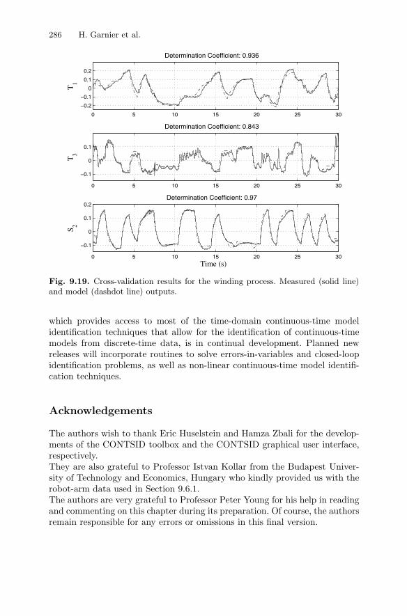
Model Validation
Cross-validation results are plotted in Figure 9.19 where it may be observedthat there is a very good agreement with quite high values for the coefficientof determination.
9.7 Conclusions
This chapter has outlined the main features of the MATLAB� CONTSIDtoolbox and illustrated its potential in practical applications. The toolbox,
286 H. Garnier et al.
0 5 10 15 20 25 30
−0.2
−0.1
0
0.1
0.2T
1
Determination Coefficient: 0.936
0 5 10 15 20 25 30
−0.1
0
0.1
T3
Determination Coefficient: 0.843
0 5 10 15 20 25 30
−0.1
0
0.1
0.2
Time (s)
S 2
Determination Coefficient: 0.97
Fig. 9.19. Cross-validation results for the winding process. Measured (solid line)and model (dashdot line) outputs.
which provides access to most of the time-domain continuous-time modelidentification techniques that allow for the identification of continuous-timemodels from discrete-time data, is in continual development. Planned newreleases will incorporate routines to solve errors-in-variables and closed-loopidentification problems, as well as non-linear continuous-time model identifi-cation techniques.
Acknowledgements
The authors wish to thank Eric Huselstein and Hamza Zbali for the develop-ments of the CONTSID toolbox and the CONTSID graphical user interface,respectively.They are also grateful to Professor Istvan Kollar from the Budapest Univer-sity of Technology and Economics, Hungary who kindly provided us with therobot-arm data used in Section 9.6.1.The authors are very grateful to Professor Peter Young for his help in readingand commenting on this chapter during its preparation. Of course, the authorsremain responsible for any errors or omissions in this final version.
9 The CONTSID toolbox for MATLAB� 287
References
1. K.J. Astrom. Introduction to Stochastic Control Theory. Academic Press, NewYork, 1970.
2. K.J. Astrom, P. Hagander, and J. Sternby. Zeros of sampled systems. Auto-matica, 20(1):31–38, 1984.
3. M. Barberi-Heyob, P.-O. Vedrine, J.-L. Merlin, R. Millon, J. Abecassis, M.-F.Poupon, and F. Guillemin. Wild-type p53 gene transfer into mutated p53 HT29cells improves sensitivity to photodynamic therapy via induction of apoptosis.International Journal of Oncology, 24:951–958, 2004.
4. T. Bastogne, H. Garnier, and P. Sibille. A PMF-based subspace method forcontinuous-time model identification. Application to a multivariable windingprocess. International Journal of Control, 74(2):118–132, 2001.
5. T. Bastogne, H. Noura, P. Sibille, and A. Richard. Multivariable identifica-tion of a winding process by subspace methods for a tension control. ControlEngineering Practice, 6(9):1077–1088, 1998.
6. T. Bastogne, L. Tirand, M. Barberi-Heyob, and A. Richard. System identifi-cation of photosensitiser uptake kinetics in photodynamic therapy. 6th IFACSymposium on Modelling and Control in Biomedical System, Reims, France,September 2006.
7. Y.C. Chao, C.L. Chen, and H.P. Huang. Recursive parameter estimation oftransfer function matrix models via Simpson’s integrating rules. InternationalJournal of Systems Science, 18(5):901–911, 1987.
8. C.F. Chen and C.H. Hsiao. Time-domain synthesis via Walsh functions. IEEProceedings, 122(5):565–570, 1975.
9. H. Dai and N.K. Sinha. Use of numerical integration methods, in N.K. Sinhaand G.P. Rao (eds), Identification of Continuous-Time Systems. Methodologyand Computer Implementation, pages 79–121, Kluwers Academic Publishers:Dordrecht, Holland, 1991.
10. H. Garnier. Continuous-time model identification of real-life processes with theCONTSID toolbox. 15th IFAC World Congress, Barcelona, Spain, July 2002.
11. H. Garnier, M. Gilson, and O. Cervellin. Latest developments for theMATLAB� CONTSID toolbox. 14th IFAC Symposium on System Identifi-cation, Newcastle, Australia, pages 714–719, March 2006.
12. H. Garnier, M. Gilson, and E. Huselstein. Developments for the MATLAB�
CONTSID toolbox. 13th IFAC Symposium on System Identification, Rotter-dam, The Netherlands, pages 1007–1012, August 2003.
13. H. Garnier, M. Gilson, P.C. Young, and E. Huselstein. An optimal IV tech-nique for identifying continuous-time transfer function model of multiple inputsystems. Control Engineering Practice, 46(15):471–486, April 2007.
14. L. Cuvillon, E. Laroche, H. Garnier, J. Gangloff, and M. de Mathelin.Continuous-time model identification of robot flexibilities for fast visual ser-voing. 14th IFAC Symposium on System Identification, Newcastle, Australia,pages 1264–1269, March 2006.
15. H. Garnier and M. Mensler. CONTSID: a continuous-time system identificationtoolbox for Matlab. 5th European Control Conference, Karlsruhe, Germany,September 1999.
16. H. Garnier and M. Mensler. The CONTSID toolbox: a MATLAB� toolboxfor CONtinuous-Time System IDentification. 12th IFAC Symposium on SystemIdentification, Santa Barbara, USA, June 2000.
288 H. Garnier et al.
17. H. Garnier, M. Mensler, and A. Richard. Continuous-time model identifica-tion from sampled data. Implementation issues and performance evaluation.International Journal of Control, 76(13):1337–1357, 2003.
18. H. Garnier, P. Sibille, and T. Bastogne. A bias-free least squares parameterestimator for continuous-time state-space models. 36th IEEE Conference onDecision and Control, San Diego, USA, Vol. 2, pages 1860–1865, December1997.
19. H. Garnier, P. Sibille, H.L. NGuyen, and T. Spott. A bias-compensating least-squares method for continuous-time system identification via Poisson momentfunctionals. 10th IFAC Symposium on System Identification, Copenhagen,Denmark, pages 3675–3680, July 1994.
20. H. Garnier, P. Sibille, and A. Richard. Continuous-time canonical state-spacemodel identification via Poisson moment functionals. 34th IEEE Conference onDecision and Control, New Orleans, USA, Vol. 2, pages 3004–3009, December1995.
21. E. Huselstein and H. Garnier. An approach to continuous-time model identi-fication from non-uniformly sampled data. 41st IEEE Conference on Decisionand Control, Las Vegas, USA, December 2002.
22. I. Kollar. Frequency Domain System Identification Toolbox Users’s Guide. TheMathworks, Inc., Mass., 1994.
23. E.K. Larsson and T. Soderstrom. Identification of continuous-time AR pro-cesses from unevenly sampled data. Automatica, 38(4):709–718, 2002.
24. L. Ljung. System Identification. Theory for the User. Prentice Hall, UpperSaddle River, NJ, USA, 2nd edition, 1999.
25. L. Ljung. Initialisation aspects for subspace and output-error identificationmethods. European Control Conference, Cambridge, UK, September 2003.
26. L. Ljung. SID: System identification toolbox for MATLAB�.http://www.mathworks.com/access/helpdesk/help/toolbox/ident/ident.shtml,2006.
27. K. Mahata and H. Garnier. Identification of continuous-time Box-Jenkins mo-dels with arbitrary time delay. Submitted to the 46th Conference on Decisionand Control, New Orleans, USA, December 2007.
28. M. Mensler, H. Garnier, and E. Huselstein. Experimental comparison ofcontinuous-time model identification methods on a thermal process. 12th IFACSymposium on System Identification, Santa Barbara, USA, June 2000.
29. M. Mensler, K. Wada. Subspace method for continuous-time system identifi-cation. 32nd ISCIE International Symposium on Stochastic Systems Theoryand Its Applications, Tottori, Japan, November 2000.
30. M. Mensler, H. Garnier, A. Richard, and P. Sibille. Comparison of sixteencontinuous-time system identification methods with the CONTSID toolbox.5th European Control Conference, Karlsruhe, Germany, September 1999.
31. M. Mensler, S. Joe, and T. Kawabe. Identification of a toroidal continu-ously variable transmission using continuous-time system identification meth-ods. Control Engineering Practice, 14(1):45–58, January 2006.
32. B.M. Mohan and K.B. Datta. Analysis of time-delay systems via shifted Cheby-shev polynomials of the first and second kinds. International Journal of Sys-tems Science, 19(9):1843–1851, 1988.
33. P.N. Paraskevopoulos. System analysis and synthesis via orthogonal polyno-mial series and Fourier series. Mathematics and Computers in Simulation,27:453–469, 1985.
9 The CONTSID toolbox for MATLAB� 289
34. A.E. Pearson and Y. Shen. Weighted least squares / MFT algorithms forlinear differential system identification. 32nd IEEE Conference on Decisionand Control, San Antonio, USA, pages 2032–2037, 1993.
35. M. Djamai, E. Tohme, R. Ouvrard, and S. Bachir. Continuous-time modelidentification using reinitialized partial moments. Application to power am-plifier modeling. 14th IFAC Symposium on System Identification, Newcastle,Australia, March 2006.
36. G.P. Rao and H. Garnier. Numerical illustrations of the relevance of directcontinuous-time model identification. 15th IFAC World Congress, Barcelona,Spain, July 2002.
37. G.P. Rao and H. Garnier. Identification of continuous-time models: direct orindirect? Invited semi-plenary paper for the XV International Conference onSystems Science, Wroclaw, Poland, September 2004.
38. G.P. Rao and H. Unbehauen, Identification of continuous-time systems, IEEProceedings - Control Theory and Applications, 153(2):185-220, March 2006.
39. S. Sagara and Z.Y. Zhao. Numerical integration approach to on-line identifi-cation of continuous-time systems. Automatica, 26(1):63–74, 1990.
40. J. Schoukens, R. Pintelon, and H. Van Hamme. Identification of linear dynamicsystems using piecewise constant excitations: use, misuse and alternatives. Au-tomatica, 30(7):1953–1169, 1994.
41. T. Soderstrom and P. Stoica. System Identification. Series in Systems andControl Engineering. Prentice Hall, Englewood Cliffs, 1989.
42. H. Unbehauen and G.P. Rao. Identification of Continuous Systems. Systemsand control series. North-Holland, Amsterdam, 1987.
43. H. Unbehauen and G.P. Rao. Identification of continuous-time systems: atutorial. 11th IFAC Symposium on System Identification, Kitakyushu, Japan,Vol. 3, pages 1023–1049, July 1997.
44. P. Van Overschee and B. De Moor. Subspace Identification for Linear Systems- Theory, Implementation, Applications. Kluwer Academic Publishers, Boston,USA, 1996.
45. P.E. Wellstead. An instrumental product moment test for model order estima-tion. Automatica, 14:89–91, 1978.
46. P.C. Young. Recursive Estimation and Time-series Analysis. Springer-Verlag,Berlin, 1984.
47. P.C. Young. Recursive estimation, forecasting and adaptive control. in C.T.Leondes (ed), Control and Dynamic Systems: Advances in Theory and Appli-cations, pages 119–166, Vol 31, Academic Press, 1989.
48. P.C. Young. Data-based mechanistic modeling of engineering systems. Journalof Vibration and Control, 4:5–28, 1998.
49. P.C. Young. The data-based mechanistic approach to the modelling, forecastingand control of environmental systems. Annual Reviews in Control, 30:169–182,2006.
50. P.C. Young. The Refined Instrumental Variable (RIV) method: unified es-timation of discrete and continuous-time transfer function models. JournalEuropeen des Systemes Automatises, in press, 2008.
51. P.C. Young and H. Garnier. Identification and estimation of continuous-timedata-based mechanistic (DBM) models for environmental systems. Environ-mental Modelling and Software, 21(8):1055–1072, August 2006.

290 H. Garnier et al.
52. P.C. Young and A.J. Jakeman. Refined instrumental variable methods of time-series analysis: Part III, extensions. International Journal of Control, 31:741–764, 1980.
53. P.C. Young, A.J. Jakeman, and R. McMurtries. An instrumental variablemethod for model order identification. Automatica, 16:281–296, 1980.


![Lecture 4: Sampling [2] XILIANG LUO 2014/10. Periodic Sampling A continuous time signal is sampled periodically to obtain a discrete- time signal as:](https://static.fdocuments.net/doc/165x107/56649da05503460f94a8bc1b/lecture-4-sampling-2-xiliang-luo-201410-periodic-sampling-a-continuous.jpg)