Identification of Technology Shocks in Structural VARs

Patrick Feve∗

University of Toulouse (GREMAQ and IDEI)

and Banque de France (Research Division)

Alain Guay

UQAM, CIRPEE and CIREQ

February, 2006

Abstract

The usefulness of SVARs for developing empirically plausible models is actually subject tomany controversies in quantitative macroeconomics. In this paper, we propose a simplealternative two step SVARs based procedure which consistently identifies and estimates theeffect of structural shocks on aggregate variables. We use the identification of the response ofhours to technology improvement as an illustration. Simulation experiments from a standardbusiness cycle model show that our approach outperforms standard SVARs. In contrast toresults with standard SVARs, the effect of the technology shocks on hours is invariant to thespecification of hours worked (level or difference). The two step procedure, when applied toactual data, predicts a short–run decrease of hours after a technology improvement followedby a delayed and hump–shaped positive response.

Keywords: SVARs, long–run restriction, technology shocks, consumption to output ratio,hours worked

JEL Class.: C32, E32

∗Address: GREMAQ–Universite de Toulouse I, manufacture des Tabacs, bat. F, 21 allee de Brienne, 31000Toulouse. email: patrick.feve@univ-tlse1.fr. We would like to thank J. Campbell, F. Collard, M. Dupaigne,A. Kurman, J. Matheron, F. Pelgrin, L. Phaneuf, F. Portier, H. Uhlig and E. Wasmer for helpful discussions. Afirst version of this paper was written when the second author was visiting the University of Toulouse. This paperhas benefited from helpful remarks during presentations at CIRANO Workshop on Structural VARs (november,2004), UQAM seminar (may, 2005) and Macroeconomic Workshop (Aix/Marseille, december 2005). The tradi-tional disclaimer applies. The views expressed herein are those of the authors and not necessary those of theBanque de France.

1

Introduction

Structural Vector Autoregressions (SVARs) have been widely used as a guide to evaluate and

develop dynamic general equilibrium models. Given a minimal set of identifying restrictions,

SVARs represent a helpful tool to discriminate between competing theories of the business cycle.

For example, Galı (1999) uses long–run restrictions a la Blanchard and Quah (1989) in a SVAR

of labor productivity and hours and shows that the response of hours to a technology shock is

persistently and significantly negative. This negative response of hours obtained from SVARs is

then implicitly employed to favor a class of business cycle models and/or reject others (see Galı

and Rabanal, 2004 and Francis and Ramey, 2004a).

The usefulness of SVARs for building empirically plausible models has been subject to many

controversies in quantitative macroeconomics (see Cooley and Leroy, 1985, Bernanke, 1986 and

Cooley and Dwyer, 1998). More recently, the debate about the effect of technology improvements

on hours worked has triggered the emergence of several contributions concerned with the ability

of SVARs to adequately measure the impact of technology shocks on aggregate variables.

Using Dynamic Stochastic General Equilibrium (DSGE) models estimated on US data as

their Data Generating Process (DGP), Erceg, Guerrieri and Gust (2004) show that the effect of a

technology shock on hours worked is not precisely estimated with SVARs. They suggest that part

of their results originate from the difficulty to disentangle technology shocks from other shocks

that have highly persistent, if not permanent, and important effects on labor productivity.1 For

example, they show that when the persistence of the non–technology shock decrease – and thus

the persistence of hours –, for a given standard error of this shock, the estimated response of

hours is less biased. Their results indicate that SVARs with long–run restriction deliver more

reliable results when the non–technology component in SVARs displays lower persistence. Their

findings also suggest to include in SVARs other variables with lower serial correlation.

Chari, Kehoe and McGrattan (2005) simulate a prototypical business cycle model estimated

by Maximum Likelihood on US data with structural shocks as well as measurement errors. They

show that the SVAR with a specification of hours in difference (DSVAR) leads to a negative

response of hours under a business cycle model in which hours respond positively. Moreover,

they show that a level specification of hours (LSVAR) does not uncover the true response of

hours and implies a large upward bias. Their findings echo some empirical evidences since

LSVAR and DSVAR models deliver conflicting responses of hours. A significant part of their

1By highly persistent and important effect, we mean that the transitory component of the variable is highlypersistent and explains a substantial fraction of its variance.

2

results originates from the inability of SVARs with a finite number of lags to properly capture

the true dynamic structure of the model. According to them, the auxiliary assumption of the

VAR that the stochastic processes for labor productivity and hours are well approximated by an

VAR with a finite number of lags does not hold. They show that this problem can be eliminated

if a relevant state variable is introduced in the SVAR. Unfortunately, the lack of observability

of such a variable (for example, capital stock and shocks) makes its use impossible. However,

even if such a meaningful variable is virtually unobserved, we can always think about observable

relevant instrumental variables that share approximatively the same dynamic structure.

Christiano, Eichenbaum and Vigfusson (2005) argue that SVARs are still a useful guide for

developing models. They find that most of the deceiving results with SVARs in Chari, Kehoe

and McGrattan (2005) come from the values assigned to the standard errors of shocks in their

economy. They notably show that when the model is more properly estimated, the standard

error of the non–technology shocks is twice lower than the standard error of the technology

shock. In such a case, the bias in SVARs with labor productivity and hours is strongly reduced.

Their findings show that the behavior of hours is closely related to the non–technology shock

and the reliability of SVARs is thus highly sensitive to the volatility of this shock. Evidence from

their simulation experiments implicitly suggests using other variables which are less sensitive

to the volatility of non–technology shocks and/or which contains a sizeable part of technology

shocks.

In light of the above quantitative findings, we propose a simple alternative method to con-

sistently estimate technology shocks and their short–run effects on aggregate variables. As an

illustration and a contribution to the current debate, we essentially concentrate our analysis

on the response of hours worked. However, our empirical strategy can be easily implemented

to other variables of interest. Although imperfect, we maintain the labor productivity variable

as a way to identify technology shocks using long–run restrictions. We argue that SVARs can

deliver accurate results if more efforts are made concerning the choice of the stationary vari-

ables. More precisely, hours must be excluded from SVARs and replaced by any variable which

presents better stochastic properties. The introduction of a highly persistent variable as hours

worked in the SVARs confounds the identification of the permanent and transitory shocks and

thus contaminates the corresponding impulse response functions. Following the previous quoted

contributions which use simulation experiments, the selected variable must satisfy the following

stochastic properties. First, the variable must display less controversies about its stationarity.2

2Pesavento and Rossi (2005) and Francis, Owyang and Roush (2005) propose other methods to deal with thepresence of highly persistent process.

3

Second, the variable must behave more as a capital variable than hours worked do, so that finite

VAR can more easily approximate the true underlying dynamics of the data. Third, the variable

must contain a sizeable technology component and present less sensitivity to highly persistent

non–technology shocks. We argue that the consumption to output ratio (in logs) is an interesting

candidate to fulfil these three requirements. The ratio is stationary and consequently displays

less persistence than hours worked. Moreover, the consumption to output ratio represents prob-

ably a better approximation of the state variables than hours worked and appears less sensitive

to transitory shocks. The first requirement can be directly found with actual data, since stan-

dard unit root tests reject the null hypothesis of an unit root. The two other requirements can

be quantitatively (through numerical experiments) and analytically deduced from equilibrium

conditions of dynamic general equilibrium models which satisfactory fit the data. In addition,

Cochrane (1994) has already shown in SVARs that the consumption to output ratio allows to

suitably characterize permanent and transitory components in GNP.

The proposed approach consists in the following two steps. In a first step, a SVAR model

which includes labor productivity growth and consumption to output ratio is considered to

consistently estimate technology shocks using with a long–run restriction. In the second step,

the impulse response functions of hours (or any other aggregate variable under interest) at

different horizons are obtained by a simple OLS regression of hours on the estimated technology

shock for different lags. We show that the impulse response functions are consistently estimated

whether hours worked are projected in level or in difference in the second step. Consequently,

our approach does not suffer from the specification choice of hours as in the standard SVAR

approach. Our method can be viewed as a combination of a SVAR approach in the line of

Blanchard and Quah (1989), Galı (1999) and Christiano, Eichenbaum and Vigfusson (2004) and

the regression equation used by Basu, Fernald and Kimball (2004) in their growth accounting

exercise.

To evaluate this proposed two step approach, we perform simulation experiments using a

standard business cycle model with a permanent technology shock and stationary preference

and government consumption shocks. This models includes three wedges that mainly explain

US aggregate fluctuations for post war period (Chari, Kehoe and McGrattan, 2004). The re-

sults show that our approach, denoted CYSVAR, performs better than the DSVAR and LSVAR

models. In particular, the bias of the estimated impulse response functions is strongly reduced.

In contrast with the results for the DSVAR and LSVAR models, we also show that the specifi-

cation of hours (in level or in difference) does not matter. Moreover, the estimated technology

shock using CYSVAR is strongly correlated with the true technology shock while weakly with

4

the non–technology shock. In other words, the estimated technology shock is not contaminated

by other shocks that drive up or down hours worked. Consequently, the estimated response of

hours obtained in the second step displays small bias. Conversely, existing approaches (DSVAR

and LSVAR) perform poorly. In particular, their estimates of the technology shock are contam-

inated by the non–technology shock. We also find in the three shock version of the model that

the CYSVAR approach which includes two variables outperforms SVARs with three variables

(productivity growth, hours and consumption to output ratio). Although the three variable

SVARs contain at least the same information (output, hours worked and consumption), this

result comes from the fact that finite autoregressions cannot properly approximate the time se-

ries behavior of hours. Consequently, hours contaminate the estimation of the technology shock

in the three variable SVAR. This supports the use a parsimonious SVARs in the first step to

consistently estimate technology shocks.

An application with US data for the period 1955Q1-2002Q4 shows that hours significantlty

decrease on impact after a positive technology shock and increase after some periods. These

results are robust to the specification of hours. The shape of the response of hours is very similar

to Basu, Fernald and Kimball (2004), Francis and Ramey (2004b), Uhlig (2004), Vigfusson (2004)

and Pesavento and Rossi (2005) who show that the negative (or almost zero) response of hours

on impact is followed by a subsequent positive response. We also investigate the sensitivity of

our results to the presence of breaks in labor productivity growth (Fernald, 2004). The impulse

response functions are qualitatively left unaffected.

The paper is organized as follows. In a first section, we briefly review some empirical results

about the effect of a technology shock on hours worked. In section 2, we present our two step

approach. The third section is devoted to the exposition of the business cycle model. Section 4

discusses in details our simulation experiments. In section 5, we present the empirical results.

The last section concludes.

1 SVARs and the Hours Worked Debate

In this section, we review some evidence about the effect of a technology shock on hours worked.

The empirical analysis uses quarterly U.S. data for the period 1955Q1-2002Q4. We use data

on logged real gross per capita product in chained 2000 dollars (yt) and logged total hours

worked per capita (ht). These series relate to the non farm business sector. As is conventional

in the literature, productivity is defined as the average labor productivity (yt − ht, in logs).

We also consider the consumption to output ratio (ct − yt, in logs). This ratio is obtained by

5

divided the nominal expenditures of non–durables and services by the nominal Gross Domestic

Product.3 Data on these three variables are reported in Figure 1. This figure shows that hours

displays a persistent downward trend from 1955 to 1980, whereas a persistent increase during

the subsequent period. Conversely, the consumption to output ratio does not display similar

patterns.

In order to assess the dynamic properties of hours and consumption to output ratio, we

first perform unit root tests. We begin by testing the null hypothesis of a unit root in these

two variables using the Augmented Dickey Fuller (ADF) test. For each variable, we regress the

growth rate on a constant, lagged level and four lags of the first difference. The ADF test statistic

is equal to -2.50 for hours and -3.18 for the consumption to output ratio. This hypothesis cannot

be rejected at the 10 percent level for hours, whereas it is rejected at the 5 percent level for the

consumption to output ratio.4 Our results on hours are thus in the line with those obtained

by Galı (1999), Galı and Rabanal (2004) and Christiano, Eichenbaum and Vigfusson (2004).

According to the ADF test, we can conclude that the consumption to output ratio is stationary

but not hours worked. It is however well known that the ADF test has very low power when the

alternative is a persistent stationary process. Therefore, we now test the null hypothesis that

hours worked series is stationary using the KPSS test.5 This test is implemented using eight lags

in the Newey and West estimator of the long–run covariance matrix. We cannot reject the null

hypothesis of stationarity at the 1 percent level, as the KPSS test statistic is 0.69.6 However,

the null hypothesis of stationarity is rejected at the 5 percent significant levels. These two unit

root tests then favor the hypothesis of the unit root for hours worked.

We now estimate Structural Vector Autoregressive (SVAR) models for four alternative spec-

ifications. In each of these specifications, we identify technology shocks as the only shocks that

can affect the long-run level of labor productivity. We first consider a bivariate LSVAR speci-

fication which includes labor productivity growth and hours in level (Christiano, Eichenbaum

and Vigfusson, 2004). We then consider a bivariate DSVAR specification in which hours are

now taken in first difference. As pointed out by Galı (1999) (2004a) and (2004b), Galı and Ra-

3The data used in our estimation are extracted from the FRED II and the BEA databases. Our dataset is thatof Galı and Rabanal (2004) and corresponds to one of the alternative measures in Christiano, Eichenbaum andVigfusson (2004). So as to define our macroeconomic variables, we use the following time series: i) gross domesticoutput of the non farm business sector (LXNFO); ii) total hours in the non farm business sector (LXNFH );iii) total non institutional civilian population over 16 (LNN ); iv) personal consumption expenditures: services(PCESV); v) personal consumption expenditures: nondurable goods (PCND) and vi) gross domestic product(GDP).

4The critical values of the ADF test statistic at 1, 5 and 10 percent significance levels are -3.49, -2.88 and-2.57.

5See Kwiatkowski et al. (1992).6The critical values of the KPSS test statistic at 1, 5 and 10 percent significance levels are 0.74, 0.46 and 0.35.

6

banal (2004) and Francis and Ramey (2004a) and suggested by the previous unit root tests, this

specification accounts for a possible non–stationarity in hours. We move beyond the bivariate

system and we now include in both the LSVAR and DSVAR specifications the consumption

to output ratio. By doing so, we want to assess the sensitivity of the results to an additional

variable in the SVAR (see Galı, 1999, Francis and Ramey, 2004a, and Christiano, Eichenbaum

and Vigfusson, 2004). Notice that this ratio is specified in level as unit root tests suggest its

stationarity.7

As is usual, we start by estimating the reduced form vector autoregression of order p

Xt = B1Xt−1 + · · · + BpXt−p + εt, Eεtε′

t = Σ. (1)

We follow Galı and Rabanal (2004) and Christiano, Eichenbaum and Vigfusson (2004) and we set

p = 4. The variable Xt includes labor productivity growth as first variable for each specification.

The other variables that enter in Xt corresponds to different SVAR specifications. Let us define

C (L) = (I − B1L − · · · −BpLp)−1, so that

Xt = C (L) εt,

where I is the identity matrix and L is the lag operator, i.e. LXt = Xt−1. The reduced form

innovations εt are linear combinations of the structural shocks ηt, i.e. εt = A0ηt, for some non

singular matrix A0. As usual, we impose an orthogonality assumption on the structural shocks,

which combined with a scale normalization implies Eηtη′

t = I2. This gives us three constraints

out of the four needed to completely identify A0. To setup the last identifying constraint,

let us define A (L) = C (L)A0. Given the ordering of Xt, we simply require that A (1) be

lower triangular, so that only technology shocks can affect the long-run level of productivity.

This amounts to imposing that A (1) is the Cholesky factor of C (1)ΣC (1)′. Given consistent

estimates of C (1) and Σ, we easily obtain an estimate for A (1). Retrieving A0 is then a simple

task using the formula A0 = C (1)−1A (1).

The impulse response functions, as well as their 95% confidence intervals,8 are reported in

Figures 2 and 3. Panel (a) of Figure 2 displays the responses of hours to a permanent technology

shock in the LSVAR specification. The response is positive and hump-shaped, though not

statistically significant. As has been previously emphasized by Chari, Kehoe and McGrattan

(2005), this LSVAR specification is essentially uninformative, since a large number of competing

7Francis and Ramey (2004a) and Christiano, Eichenbaum and Vigfusson (2004) include this cointegrationrelationship between consumption and output in their SVARs.

8These confidence intervals are computed by standard bootstrap methods, using 1000 draws from the sampleresiduals.

7

DSGE models could produce responses contained in the confidence interval. Panel (b) of Figure

2 displays the responses of hours to a permanent technology shock in the DSVAR specification.

Hours fall during two periods and the response remain negative for each horizon. Notice that the

response is statistically significant on impact, as well as one period after the shock. These results

are consistent with the empirical evidence reported in Galı (1999) and Galı and Rabanal (2004).

Panels (a) and (b) of Figure 3 report the responses of hours in a three–variables system. Most

of the quantitative patterns are left unaffected by the three–variables system. In the LSVAR

specification (see panel (a) of Figure 3), the response of hours is still hump-shaped but not

precisely estimated. The main difference concerns the impact response which becomes slightly

negative, although not significant. For the DSVAR specification, the response of hours to a

positive technology shock is negative during four periods, but not significantly different from

zero.

In conclusion to this section, empirical evidence reports conflicting results about the effect

of a technology shock on hours worked. The level specification displays a positive hump–shaped

response whereas the difference specification implies a decrease in hours. Notice that the three–

variables system does not help so much as most of the conflicting results are maintained. Chris-

tiano, Eichenbaum and Vigfusson (2004) provide similar evidence using six–variables SVARs. In

their LSVAR specification, the response of hours is positive, although not precisely estimated,

while the response is negative in the DSVAR specification. The conflicting results mainly orig-

inate from the specification of hours. The problem remains unsolved: which specification of

hours to adopt in SVARs? Since hours are highly persistent, we can not determine using unit

root tests in small sample which specification to adopt. In the next section, we will propose a

simple two–step approach which does not suffer from the problem resulting from the time series

properties of hours worked.

2 The Two Step Approach

The goal of our approach is to accurately identify the technology shocks in the first step using an

adequate stationary variable in the VAR model. A large part of the performance of the two step

approach depends on the time series properties of this variable. This latter can be interpreted as

an instrument allowing to retrieve with more precision the true technology shock. The variable

choice is motivated in part by simulation results in Erceg, Guerrieri and Gust (2004), Chari

Kehoe and McGrattan (2005) and Christiano, Eichenbaum and Vigfusson (2005). They show

that, when hours worked are contaminated by an important persistent transitory component,

the SVAR performs poorly in their experiments. In an interesting paper, Chari, Kehoe and

8

McGrattan (2004) propose a method in order to account for economic fluctuations based on the

measurement of various wedges. They assess what fraction of the output fluctuations can be

attributed to each wedge separately and in combinations. For the postwar period, the efficiency

and labor wedges are proeminent to explain output movement. Investment wedge plays a minor

role in the postwar period and especially at low frequencies of output fluctuations. They also

find that the government consumption component accounts for an insignificant fraction of fluc-

tuations in output, labor, consumption and investment which is compatible with the results in

Burnside and Eichenbaum (1996). The results in Chari Kehoe and McGrattan (2004) suggest

that the observed fluctuations and persistence of hours worked depend on an important portion

of the labor wedge. In contrast, in their prototypical economy, the consumption-output ratio is

less dependent on labor wedge and is much more sensitive to the government consumption wedge.

However, this wedge appears to be negligible in the dynamic of real variables such as consump-

tion and output. As a consequence, the transitory component of the consumption-output ratio

is then probably less important than the one corresponding to the permanent shock. According

to this, the consumption-output ratio is a more promising variable to use in a VAR for identi-

fying technology and non-technology and their respective impulse responses than hours worked.

Cochrane (1994) also argues that the consumption to output ratio contains useful information

to disentangle the permanent to the transitory component. Moreover, in data, we can reject the

unit root for this ratio and the empirical autocorrelation function is clearly less persistent that

the one for hours. So we decide to introduce this ratio as instrument to identify the technology

shocks. With this identified shocks at the first step, we can then evaluate the impact of these

shocks on a variable of interest (for example, hours) in the second step.

Step 1: Identification of technology shocks

We consider a VAR model which includes productivity growth and consumption to output ratio

(in logs). We start by specifying a VAR(p) model in these two variables:(

∆ (yt − ht)ct − yt

)=

p∑

i=1

Bi

(∆ (yt−i − ht−i)

ct−i − yt−i

)+ εt (2)

where εt = (ε1,t, ε2,t)′ and E(εtε

′

t) = Σ. Under usual conditions, this VAR(p) model admits a

VMA(∞) representation (∆ (yt − ht)

ct − yt

)= C(L)εt

where C(L) = (I2 −∑p

i=1BiL

i)−1. The SVAR model is represented by the following VMA(∞)

representation (∆ (yt − ht)

ct − yt

)= A(L)

(ηT

t

ηNTt

)

9

where ηTt is period t technology shock, whereas ηNT

t is period t non–technology shocks. By

normalization, these two orthogonal shocks have zero mean and unit variance. The identifying

restriction implies that the non–technology shock has no long–run effect on labor productivity.

This means that the upper triangular element of A(L) in the long run must be zero, i.e. A12(1) =

0. In order to uncover this restriction from the estimated VAR(p) model, the matrix A(1) is

obtained as the Choleski decomposition of C−1(1)ΣC−1(1)′. The structural shocks are then

directly deduced up to a sign restriction:

(ηT

t

ηNTt

)= (C(1)A(1))−1

(ε1,t

ε2,t

)

We argue that replacing hours by the consumption to output ratio can help to identify more

accurately the true technology shocks. In contrast to hours worked, the consumption to output

ratio is probably less contaminated by important persistent transitory shocks. Its use in the

SVAR model can reduce the confusion of the the true permanent technology shocks with the

transitory shocks.

Step 2: Estimation of the responses of hours to a technology shock

Suppose the following infinite moving average representation for hours worked as a linear function

of a technological and a non-technological shocks:

ht = a21(L)ηTt + a22(L)ηNT

t . (3)

where the individual a21,k measures the impact of the technology shock at lag k. The identifying

restriction of Step 1 implies that non–technology shocks are orthogonal to technology shocks by

construction, i.e. E(ηTt−i, η

NTt−j) = 0 ∀i, j and that the technology and non–technology shocks

are serially uncorrelated which implies E(ηTt , ηT

t−i) = 0 and E(ηTt , ηT

t−i) = 0 ∀i 6= 0,

Let ηTt denotes the estimated technology shock obtained from the SVAR model in the first

step. According to the debate on the right specification of hours worked, we examine three

specifications to measure the impact of technology on this variable. In the first specification,

hours series is projected in level on the identified technology shocks while in the second specifi-

cation, hours series is projected in difference. Finally, in the third specification, the hours series

is projected on its own first lag and the identified technology shocks. This latter specification is

more flexible in the sense that we do not impose a unit root but we allow to the AR(1) parameter

to be freely estimated. The first and the second specifications are in fact a restricted version of

the third with an AR(1) parameter restricted to be zero or one.

10

Let us now present in more details the three specifications. In the first one, we regress the

logs of hours worked on the current and past values of the identified technology shocks ηTt in

the first-step:

ht =

q∑

i=0

θiηTt−i + νt (4)

where q < +∞. νt is a composite error term that accounts for non–technology shocks and the

remainder technology shocks.

A standard OLS regression provides the estimates of the population responses of hours to

the present and lagged values of the technology shocks, namely:

a21,k = θk.

Hereafter, we refer to this approach as CYSVAR-h. According to the debate on the appropriate

specification of hours, this variable is regressed in first difference on the current and past values

of the identified technology shocks. Hereafter, we refer to this approach as CYSVAR-∆h. The

response of hours worked to a technology shock is now estimated from the regression:

∆ht =

q∑

i=0

θiηTt−i + νt. (5)

As hours are specified in first difference, the estimated response at horizon k is obtained from

the cumulated OLS estimates:

a21,k =k∑

i=0

θi

Finally, an interesting avenue is to adopt a more flexible approach by freely estimating the

autoregressive parameter of order one for hours. This lets the data discriminate between the

presence of an unit root in the stochastic process of hours worked. Hereafter, we refer to this

approach as CYSVAR-AR(1). The response to a technology shock is now estimated from the

regression of hours on one lag of itself and lags of the technology shock:

ht = ρht−1 +

q∑

i=0

˜θiη

Tt−i + ˜νt. (6)

The estimated response at horizon k is obtained from the OLS estimates of ρ and θi (i = 1, ..., q):

a21,k =k∑

i=0

ρi θk−i.

In the following proposition, we show that the OLS estimators of the effect of technology

shocks are consistent estimators of the true ones for the three specifications.

11

Proposition 1 Assume the infinite moving average representation (3) for hours worked and

consider the estimation of the finite VAR in the first step as defined in (2) and the three projec-

tions (4), (5) and (6) in the second step. The OLS estimators a21,k converge in probability to

a21,k for the three specifications, ∀k.

The proof is given in Appendix A.

In Proposition 1, the property of consistency is derived under the assumption that hours

worked follow a stationary process. While the specification of hours in difference could provide

a good statistical approximation of this variable in small sample, hours worked per capita are

bounded and therefore the stochastic process of this variable cannot have a unit root asymptot-

ically. By definition, the consistency property of an estimator is an asymptotically concept so

only the asymptotic behavior of hours worked is of interest. Consequently, the consistency of

the OLS estimators for the three specifications is derived only under the assumption that hours

worked per person is a stationary process. It is worth noting that the specification of hours

(level or first difference) does not asymptotically matter. However, the small sample behavior

of the three specifications can differ.

Confidence intervals of impulse response functions are computed using a consistent estimator

of the asymptotic variance-covariance of the second step parameters. Newey (1984) shows how

to derive such a consistent estimator of the asymptotic variance-covariance matrix. In particular,

he shows how a two step procedure such as ours can be represented as member of method of

moments estimators. With this representation in hand, he derives the asymptotic variance-

covariance matrix of the second step estimator. This asymptotic variance-covariance matrix

takes into account the generated regressors problem occurring in the first step and allows for

unknown serial dependence of the residuals in the second step. In Appendix B, we provide more

details on the implementation and computation of the consistent estimator proposed by Newey

(1984) for the asymptotic variance-covariance matrix of our two step estimator.

3 A Business Cycle Model

We consider a standard business cycle model that includes three shocks. The utility function of

the representative household is given by

Et

∞∑

i=0

βi (log (Ct+i) + ψ χt+i log (1 − Ht+i))

where β ∈ (0, 1) denotes the discount factor and ψ > 0 is a time allocation parameter. Et is the

expectation operator conditional on the information set available at time t. Ct and Ht represent

12

consumption and labor supply at time t. The labor supply Ht is subjected to a preference shock

χt, that follows a stationary stochastic process.

log(χt) = ρχ log(χt−1) + (1 − ρχ) log χ + σχεχ,t

where χ > 0, |ρχ| < 1, σχ > 0 and εχ,t is iid with zero mean and unit variance. As noted by

Galı (2005), this shock can be an important source of fluctuations as it accounts for persistent

shifts in the marginal rate of substitution between goods and work (see Hall, 1997). Such shifts

capture persistent fluctuations in labor supply following changes in labor market participation

and/or changes in the demographic structure. Additionally, this preference shock allows us to

simply account for other distortions on the labor market, labelled labor wedge in Chari, Kehoe

and McGrattan (2004). For example, they show that a sticky-wage economy or a real economy

with unions will map it into a simple model economy with this type of shock. Note that this

shock is observationally equivalent to a tax shock on labor income.

The representative firm use capital Kt and labor Ht to produce a final good Yt. The technol-

ogy is represented by the following constant returns–to–scale Cobb–Douglas production function

Yt = Kαt (ZtHt)

1−α

where α ∈ (0, 1). Zt is assumed to follow an exogenous process of the form

log(Zt) = log(Zt−1) + γz + σzεz,t

where σz > 0 and εz,t is iid with zero mean and unit variance. In the terminology of Chari,

Kehoe and McGrattan (2004), Z1−αt in the production function corresponds to the efficiency

wedge. This wedge may capture for instance input-financing frictions. Capital stock evolves

according to the law of motion

Kt+1 = (1 − δ)Kt + It

where δ ∈ (0, 1) is a constant depreciation rate. Finally, the final output good can be either

consumed or invested

Yt = Ct + It + Gt

where Gt denotes government consumption. We assume that gt = Gt/Zt evolves according to

log(gt) = ρg log(gt−1) + (1 − ρχ) log g + σgεg,t

where g > 0, |ρg| < 1, σg > 0 and εg,t is iid with zero mean and unit variance. This shock,

labelled government consumption wedge, is for example equivalent to persistent fluctuations in

13

net exports in an open economy. The model is thus characterized by three time varying wedges,

i.e. the efficiency, labor and government consumption wedges, that summarize a large class of

mechanisms without having to explicitly specify them.

To analyze the quantitative implications of the model, we first apply a stationary–inducing

transformation for variables that follow a stochastic trend. Output, consumption, investment

and government consumption are divided by Zt, and the capital stock is divided by Zt−1. The

approximate solution of the model is computed from a log–linearization of the stationary equi-

librium conditions around the deterministic steady state.

The parameter values are familiar from business cycle literature (see Table 1). We set the

capital share to α = 0.33 and the time allocation parameter ψ = 2.5. We choose the discount

factor so that the steady state annualized real interest rate is 3%. We set the depreciation rate

δ = 0.015. The growth rate of Zt, namely γz, is equal to 0.0036. The share of government

consumption in total output at steady state is either 0 or 20%, depending on the version of

the model we consider. The parameters of the three forcing variables (Zt, Gt, χt) are borrowed

from previous empirical works with US data. The standard–error σz of the technology shock is

equal to 1% (see Prescott, 1986, Burnside and Eichenbaum, 1996, Chari, Kehoe and McGrattan,

2005 and Christiano, Eichenbaum and Vigfusson, 2005). Following Christiano and Eichenbaum

(1992) and Burnside and Eichenbaum (1996), the autoregressive parameter ρg of government

consumption is set to 0.95. The standard error σg is set to 0.01 or 0.02. These two values

include previous estimates. We choose alternative values (0.90;0.95;0.99) for the autoregressive

parameter ρχ of the preference shock. Previous estimations (see Chari, Kehoe and McGrattan,

2005 and Christiano, Eichenbaum and Vigfusson, 2005) suggest value between 0.95 and 0.99,

but we add ρχ = 0.90 for a check of robustness. Finally, the standard error of this shock

σχ takes three different values (0.005;0.01;0.02). These values roughly summarize the range of

previous estimates (see Erceg, Guerrieri and Gust, 2004, Chari, Kehoe and McGrattan, 2005,

and Christiano, Eichenbaum and Vigfusson, 2005). The alternative calibrations summarize

previous estimates which use different datasets and estimation techniques. They allow us to

conduct a sensitivity analysis and to evaluate the relative merits of different approaches for

various calibrations of the forcing variables.

4 Simulation Results

In our Monte–Carlo study, we generate 1000 data samples from the business cycle model. Every

data sample consists of 200 quarterly observations and corresponds to the typical sample size of

14

empirical studies. In order to reduce the effect of initial conditions, the simulated samples include

100 initial points which are subsequently discarded in the estimation. For every data sample, we

estimate VAR models with four lags as in Erceg, Guerrieri and Gust (2004), Chari, Kehoe and

McGrattan (2005), and Christiano, Eichenbaum and Vigfusson (2005). We consider two versions

of the model, depending on the number of shocks included. The two shocks version includes

technology shock and preference shocks, whereas the three shocks version adds government

consumption. The two shocks version is used so as to evaluate various SVARs with two variables.

The three shocks version allows to assess the reliability of three variable SVARs. Moreover, we

want to verify if our two step approach properly uncovers the true response of hours when a

stationary shock to government consumption affects persistently the consumption to output

ratio.

For each experiment, we investigate the reliability of different SVARs based on identification

of technology shocks: i) a DSVAR models with labor productivity growth and hours in first

difference; ii) a LSVAR model with labor productivity growth and hours in level; iii) CYSVAR–

h approach in which the SVAR model includes labor productivity growth and consumption to

output ratio in the first step and hours are regressed on the estimated technology shock in the

second step. The specification of CYSVAR–∆h and CYSVAR–AR(1) are the same in the first

step, but they consider hours in first difference and lagged hours in the second step (see Section

2 for more details). In the second step of the CYSVAR approach, we consider current and twelve

lagged values of the identified (in the first step) technology shocks.9

4.1 Results from the two shock model

Figures 4 and 5 display the responses of hours for each SVARs in our baseline calibration

(ρχ = 0.95 and σz = σχ = 0.01). The solid line represents the response of hours in the model,

whereas the dotted line corresponds to the estimated response from SVARs.

The response of hours obtained from the DSVAR model displays a large downward bias

(see figure 4–(a)), and it is persistently negative. This result is similar to Chari, Kehoe and

McGrattan (2005) who show that the difference specification of hours adopted by Galı (1999),

Galı and Rabanal (2004) and Francis and Ramey (2004a) can lead to mistaken conclusions about

the effect of a technology shock. Note that a DSVAR model is obviously misspecified under the

business cycle model considered here, as it implies an over–differentiation of hours. The first

difference specification of hours can create distortions and lead to biased estimated responses.

However, Chari, Kehoe and McGrattan (2005) show that SVARs with hours in quasi–difference,

9We also investigate different lagged values of the technology shock and the main results are left unaffected.

15

consistent with the business cycle model, display similar patterns.

The responses of hours obtained from a LSVAR model displays a large upward bias, as the

estimated response on impact is almost twice the true response and is persistently above the

true response (see Figure 4–(b)). These results are again in the line with those of Chari, Kehoe

and McGrattan (2005) and to a lesser extent similar with those of Christiano, Eichenbaum and

Vigfusson (2005). As reported by Chari, Kehoe and McGrattan (2005), confidence intervals with

the LSVAR model are very large and therefore not informative. The LSVAR cannot discriminate

between a model with a positive or a negative effect of the technology shock on impact.10

Consider now the CYSVAR–h approach. Figure 5–(a) shows that this approach delivers

reliable estimates of the response of hours. The bias is small, especially in comparison with

the ones from the DSVAR and LSVAR. Another interesting result is that the three CYSVAR

approaches deliver very similar results (see Figures 5–(a), (b) and (c)). Therefore, our two step

approach does not suffer from the specification of hours, contrary to the DSVAR and LSVAR.

This result is consistent with Proposition 1. As for the LSVAR, the confidence intervals for

CYSVAR–h are large. Interestingly, the confidence intervals for CYSVAR–∆h and CYSVAR–

AR(1) are narrower on impact than for the LSVAR model. In particular, an one-sided test rejects

the hypothesis that the response on impact is negative at the 5% level. These two specifications

can then reject an alternative model in which hours decreases on impact after a technology

improvement. In contrast, as mentioned by Chari, Kehoe and McGrattan (2005), the LSVAR is

incapable of differentiating between alternative models with starkly different impulse response

functions.

To evaluate the size of the bias, Table 2 reports the cumulative absolute bias between the

average response in SVARs and the true response over different horizons.11 In this table, we

report only simulation results with the CYSVAR–AR(1) approach since these results are invari-

ant to the specification of hours. Our benchmark calibration corresponds to the second panel

in Table 2 when ρχ = 0.95 and σχ/σz = 1. We also obtained a large bias with DSVAR and

LSVAR models (both on impact and for different horizons). However, The CYSVAR–AR(1)

delivers very reliable results compared with DSVAR and LSVAR. We also investigate other cal-

10These very large confidence intervals are not surprising, as long run effects of shocks involve a reliable estimateof the sum of the VAR parameters. The convergence of the least-squares estimator for the VAR does not implyan accurate approximation of the long run effect (see Sims 1972, Faust and Leeper, 1996 and Potscher, 2002).The lack of precision of the estimated long run effect is then translated to the impulse response functions.

11This measure is defined as cmd(k) =∑k

i=0|irfi(model) − irfi(svar)| where k denotes the selected horizon,

irfi(model) the RBC impulse response and irfi(svar) = (1/N)∑N

j=1irfi(svar)j the mean of impulse responses

over the N simulation experiments obtained from a SVAR model. In fact, the cmd measures the area of the biasup to the horizon k.

16

ibration of (ρχ, σχ). When the standard error σχ of the non–technology shock is smaller, the

accuracy of the LSVAR and DSVAR models increases (see the cases where σχ/σz = 0.5) and

the LSVAR model and the CSVAR–AR(1) approach deliver very similar results. Conversely,

when the standard error σχ of the preference increases, the LSVAR and DSVAR models poorly

identify the effect of a technology shock on hours (see the cases σχ/σz = 2). In this latter case,

the CSVAR approach tends to over–estimate the true effect of the technology shock, but the cu-

mulative absolute mean bias remains small compared to the LSVAR and DSVAR models. Table

2 displays another interesting result: when the persistence of the preference shock increases from

0.9 to 0.99, the bias decreases. For the DSVAR model, this result can be partly explained by

a decrease in distortions created by over–differentiation. For the CYSVAR approach, the bias

reduction mainly originates from the effect of the preference shock on hours and consumption

to output ratio.

To better understand these last results, we investigate the effect of ρχ and σχ on the structural

autoregressive moving average representation of hours and consumption to output ratio. For

our baseline calibration (ρχ = 0.95, σz = σχ = 0.01), we obtain:

log(Ht) = cst + 0.35361

(1 − 0.9622L)σzεz,t − 1.5240

(1 − 0.9759L)

(1 − 0.9622L)(1 − 0.95L)σχεχ,t

log(Ct) − log(Yt) = cst − 0.42201

(1 − 0.9622L)σzεz,t + 0.8180

(1 − 0.9928L)

(1 − 0.9622L)(1 − 0.95L)σχεχ,t,

where cst is an appropriate constant. The non–technology component is larger for hours than

for consumption to output ratio. In this case, the preference shock accounts for 91% of variance

of hours, whereas it represents 63% of the variance of the ratio. Moreover, the persistence

of hours generated by the preference shock is more pronounced. This can be seen from the

ARMA(2,1) representation of hours and consumption to output ratio. The two series display

the same autoregressive parameters, which are associated to the dynamics of capital and the

persistence of the preference shock. However, the moving average parameter differs. In the case

of hours, the parameter is equal to −0.976, whereas it is −0.993 for the consumption to output

ratio. Figure 6 illustrates this property and reports the autocorrelation function of these two

variables due to the preference shock. We see that the autocorrelations of the consumption to

output ratio are smaller than the ones of hours. The labor wedge has therefore a greater impact

in terms of volatility and persistence on hours than on consumption to output ratio. When the

standard error of the preference shock is reduced (σχ = 0.005), its contribution to the variance

decreases, it becomes 73% for hours and 30% for the consumption to output ratio. In this

case, SVARs have less difficulty to disentangle technology shocks from other shocks that have

17

highly persistent, if not permanent effects on labor productivity. This explains why SVARs can

properly uncover the true IRFs of hours to a technology shock.

To assess the effect of a highly persistent preference shock, we now set ρχ = 0.99. This

situation is of quantitative interest as Christiano, Eichenbaum and Vigfusson (2005) obtain

values for this parameter between 0.986 and 0.9994. In this case, the ARMA representation

becomes:

log(Ht) = cst + 0.35361

(1 − 0.9622L)σzεz,t − 1.2710

(1 − 0.9737L)

(1 − 0.9622L)(1 − 0.99L)σχεχ,t

log(Ct) − log(Yt) = cst − 0.42201

(1 − 0.9622L)σzεz,t + 0.5167

(1 − 0.9960L)

(1 − 0.9622L)(1 − 0.99L)σχεχ,t.

The roots of moving average and the autoregressive parameters related to the preference shock

in the expression of the consumption to output ratio are very similar,12 so its dynamics can be

approximated by a first order autoregressive process:

(log(Ct) − log(Yt)) ≃ cst + 0.9622(log(Ct−1) − log(Yt−1)) − 0.4220σzεz,t + 0.5167σχεχ,t.

The consumption to output ratio behaves like the deflated capital. Conversely, hours do not share

this property and finite autoregressions cannot properly uncover its true dynamics. This is illus-

trated in Figure 7 which reports the autocorrelation function of hours, consumption to output

ratio and capital deflated by the total factor productivity. As emphasized by Chari, Kehoe and

McGrattan (2005), one of the problem with a SVAR model is that it does not included capital–

like variable. In the model, the corresponding relevant state variable is log(Kt/Zt−1). Since Zt

is not observable in practice and Kt is measured with errors, we cannot include log(Kt/Zt−1) in

SVARs. As can be seen from Figure 7, the autocorrelation functions of (C/Y ) and (K/Z) are

very close, but the ones of hours differ sharply.

This latter result suggests that the consumption to output ratio can be a good proxy of

the relevant state variable when shocks to labor supply are very persistent or non-stationary.

Conversely, hours cannot display this pattern. Highly persistent or non–stationary labor supply

shocks is of course debatable but empirical works support this specification in small sample

(see Gali, 2005, Christiano, Eichenbaum and Vigfusson, 2005 and Chang, Doh and Schorfheide,

2005). To better understand the results under a close to non–stationary labor supply, we report

in appendix C some calculations about the dynamic behavior of the consumption to output ratio

12When we set ρχ = 0.999, this finding is strengthened. Regarding only the effect of the preference shock, thereduced form of the consumption to output ratio is log(Ct) − log(Yt) = 0.3733(1 − 0.9993L)(1 − 0.9622L)−1(1 −0.999L)−1σχεχ,t.

18

and hours for an economy with non stationary labor supply shocks. We notably show that when

preference shocks follow a random walk (and thus hours are non–stationary), the consumption

to output ratio follows an autoregressive process of order one with an autoregressive parameter

exactly equal to the one of the deflated capital. Conversely, the growth rate of hours follows an

ARMA process which can be poorly approximated by finite autoregressions. Note that a SVAR

model with long–run restrictions that includes labor productivity growth and the consumption

to output ratio is valid whatever the process (stationary or non-stationary) of the hours series.

The CYSVAR approach allows us to abstract from the very sensitive specification choice of

hours in SVARs.

Simulation results for the cumulative absolute bias are completed with a measure of uncer-

tainty about the estimated effect of the technology shocks. We thus compute the cumulative

Root Mean Square Errors (RMSE) at various horizons.13 The RMSE accounts for both bias and

dispersion of the estimated IRFs. The results are reported in Table 3. Simulation experiments

for different calibrations show again that the CSVAR approach provides smaller RMSE than the

LSVAR and DSVAR models. This result comes essentially from the smaller bias with CSVAR.

The large RMSE of DSVAR mainly originates from the large bias. In consequence, DSVAR

model displays IRFs that are strongly biased but more precisely estimated. In contrast, LSVAR

model displays smaller bias of IRFs but larger dispersion than DSVAR. The CSVAR approach

presents the smallest bias on estimated IRFs and the estimated responses are more precisely

estimated in comparison with LSVAR. These results from RMSE suggest favoring CYSVAR to

LSVAR and DSVAR.

Finally, to judge the identification of the structural shocks, we compute the correlation

between the estimated shock and the true shock of the various version of the business cycle

model. More precisely, we first compute the correlation between the estimated (from SVARs)

and the true technology shocks, namely: Corr(εz, ηT ), where εz denotes the true technology

shock and ηT is the estimated technology shock from SVARs. We also compute Corr(εχ, ηT ), the

correlation between the estimated technology shock and non–technology shock εχ of the business

cycle model. The idea is that if any method is able to consistently estimate the technology shock,

we must obtain Corr(εz, ηT ) ≈ 1 and Corr(εχ, ηT ) ≈ 0. These correlations are reported in Table

4. The CYSVAR approach always delivers the highest Corr(εz, ηT ). This correlation is relatively

high, as it always exceeds 0.9 and it is not very sensitive to changes in (σz, ρχ, σχ). Conversely,

13This measure is defined as crmse(k) =∑k

i=0rmsei where k denotes the selected horizon, rmsei =

((1/N)∑N

j=1(irfi(model) − irfi(svar)j)2)1/2 the RMSE at horizon i, irfi(model) the RBC impulse response

function of hours and irfi(svar)j the SV AR impulse responses function of hours for the jth draw and N is thenumber of simulation experiments.

19

this correlation is lower in the case of the DSVAR model and it decreases dramatically with the

volatility of the preference shock. For example, when σχ = 2σz and ρχ = 0.99, the correlation is

0.65 for the DSVAR model, in comparison with 0.91 for the CYSVAR approach. The LSVAR

delivers better results that the DSVAR, but it never outperforms the CYSVAR approach.

Let us now examine the correlation between the identified technology shocks of the true

preference shocks, namely: Corr(εχ, ηNT ). The CYSVAR approach always delivers the lowest

correlation (in absolute value). In the case of the DSVAR model, this correlation becomes large

(Corr(εχ, ηT ) ≈ 0.72) when the variance of the preference shock increases. The large correlation

allows to explain why the DSVAR model estimates a negative response of hours to a technology

shock. Indeed, the estimated technology shock is contaminated by the preference shock. Hours

worked persistently decrease after this shock in the model. It follows that the DSVAR model

erroneously concludes that hours drop after a technology shock. A similar result applies in the

case of the LSVAR model: the correlation between the estimated technology shock and the

true non–technology shock is negative.14. This explains why the LSVAR model over–estimates

the effect of a technology shock. In contrast, the CYSVAR approach does not suffer from this

contamination.

4.2 Results from the three shock model

We first investigate the reliability of SVARs which include two variables (labor productivity

and hours for LSVAR and DSVAR models; labor productivity and consumption to output ratio

for our two step approach). Figure 8 displays the responses of hours for each SVAR using our

baseline calibration (ρχ = ρg = 0.95, σz = σχ = σg = 0.01). As in the case of two shocks,

the response of hours obtained from the DSVAR model is downward biased (see Figure 8–(a))

and persistently negative. The response of hours from the LSVAR model is upward biased and

the CYSVAR approach delivers again more reliable results. This is confirmed in the first panel

of Table 5. For the two values of σg = (0.01; 0.02), the CYSVAR approach outperforms the

DSVAR and LSVAR models. Notice that increasing the size of the government consumption

shock does not deteriorate the reliability of the two step approach.

From our three shock model, we assess the DSVAR and LSVAR when they include three

variables (labor productivity, hours and consumption to output ratio). Figure 9 reports the

responses of hours for the three approaches. Figures 9–(a) and 9–(b) show that SVAR models

that include three variables deliver better results. The downward bias of the DSVAR is reduced,

as the response on impact becomes positive. Moreover, the upward bias of the LSVAR decreased.

14When σχ = 2 × σz, the LSVAR model provides Corr(εχ, ηT ) ≈ −0.40.

20

However, the DSVAR and LSVAR models do not uncover the true response of hours. These

results are in the line with those of Chari, Kehoe and McGrattan (2005). In our experiments,

the CYSVAR approach largely outperforms the DSVAR and LSVAR models (see Table 5). At

a first glance, this result is surprising, as a SVAR model which includes labor–productivity and

consumption to output ratio (CYSVAR) must a priori contain the same information as a SVAR

with labor–productivity, hours and consumption to output ratio (LSVAR). Our findings mainly

originate in the fact that finite order autoregression cannot properly represent the time series

behavior of hours as implied by the model. It follows that hours in SVAR contaminates the

estimation of IRFs, even if the consumption to output ratio is included in the VAR model.

These results suggest eliminating hours from SVAR models if the objective is to consistently

identify technology shocks.

We also report in Table 6 the correlation between the estimated technology shock and the true

shock of the business cycle model. We do not report the correlation with individual stationary

shocks as we cannot separately identify each of them. The CYSVAR approach delivers again the

highest Corr(εz, ηT ). This correlation is relatively high, as it always exceeds 0.9 and it is not

very sensitive to changes in σg. Conversely, the LSVAR model with three variables provides the

lowest correlation, around 0.83. Interestingly, the DSVAR model with three variables performs

better than the DSVAR with two variables as the correlation increases from 0.77 to 0.91.

Finally, we evaluate the relative performance of our approach in comparison with the LSVAR

and DSVAR models which use the alternative nonparametric estimator of the long-run covariance

matrix proposed by Christiano, Eichenbaum and Vigfusson (2005). In most cases, the CYSVAR

approach still outperforms the LSVAR and DSVAR models.We decide not to report those results

because the use of this alternative estimator raises two problems. First, this way of proceed is not

conceptually consistent with the fundamental relation between the structural and the reduced

form. Indeed, the estimator of the matrix A0 allowing to retrieve the structural shocks from the

reduced form shocks does not respect the following relation A0A0′ = Σ between the structural

and the reduced forms. Consequently, it seems to us very difficult to interpret such results.

Second, the bandwidth parameter is arbitrarily fixed to 150 for a sample of 180 observations

(!!!). Such estimator of the long run covariance matrix needs to fulfill conditions to be consistent.

In particular, the bandwidth parameter for the Bartlett kernel needs to grow at a rate which

does not exceed T 1/3 where T is the number of observations.15 This condition is clearly violated

15Alternative consistent data-driven procedure to choose the bandwidth parameter can be used as proposed byNewey and West (1994), among others.

21

for a bandwidth parameter equals to 150, consequently their estimator is not consistent.16

5 Application of the Two Step Approach

We first present our empirical results with the two step approach. Second, we investigate the

effects of breaks in labor productivity.

5.1 Findings

We now apply our methodology to US data (see the first section). We first estimate a bivariate

VAR model with four lags that includes productivity growth and the log of consumption to

output ratio. We then identify the technology shock using the long run restriction that only this

shock can have a long run effect on labor productivity. Technology shock leads to a permanent

increase in labor productivity, while the consumption to output ratio decreases in the short run,

illustrating the smoothness of consumption. As pointed out by Francis and Ramey (2004a), an

important issue concerns the response of labor productivity to the non–technology shock. Fran-

cis and Ramey (2004a) show that the impulse response functions from LSVAR model indicate

that non–technology shocks have a very persistent and significant effect on labor productivity.

The estimated responses from LSVAR are thus inconsistent with the fundamental identifying

assumption. In contrast, the DSVAR specification used by Galı (1999) and Francis and Ramey

(2004a) does not display this pattern. With the CYSVAR model, the response of labor produc-

tivity to a non–technology shock is short–lived as it vanishes after 12 periods and is statistically

not different from zero after three periods. Our approach is thus consistent with the basic iden-

tifying assumption that this shock cannot have a permanent effect on labor productivity. This

is again a direct consequence of the use of the consumption to output ratio instead of hours in

the SVAR model.

Using the estimated value of the technology shock, we estimate the response of hours by OLS

regressions. We consider the specification CYSVAR–AR(1). The impulse response functions,

as well as their 95% confidence intervals, are reported in Figure 10. The confidence intervals

are computed using the formula presented in Appendix B. On impact, hours worked decrease

after a technology shock. After three periods, the response becomes persistently positive and

16As shown in the simulations, the LSVAR overestimates the impact effect of the technology on hours worked.For a choice of the bandwidth parameter too large, the nonparametric estimator of the spectral density at zerofrequency with the Bartlett window is known to be downward biased (see Hauser, Potscher, and Reshenhofer,1999). For this reason, the choice of a bandwidth equal to 150 decreases the bias of the estimated impact inthe simulations. However, for an economy with only the technology and the government spending shocks, thestandard LSVAR underestimates the impact of the technology on hours worked. In this case, the procedure usingthe nonparametric estimator with 150 lags amplifies the underestimation of the impact effect which is consistentwith the downward bias of this estimator for a large bandwidth as mentioned above.

22

hump–shaped. The 95% confidence interval suggests that the response of hours on impact is

significantly different from zero. However, the positive hump–shaped response of hours is not

precisely estimated.

The shape of the response of hours is very similar to what Basu, Fernald and Kimball

(2004) obtain with US annual data. Our first step differs from theirs, as we use a SVAR

model with a long–run restriction, whereas they construct a measure of aggregate technology

change, controlling for imperfect competition, varying utilization of factors and aggregation

effects. However, our second step shares the same methodology since the effect of technology

improvement is measured by a simple regression of hours on lags of itself and the estimated

technology shock.17 They find that total hours worked fall significantly on impact. During

the subsequent years, hours recover sharply. However, the response of hours is not precisely

estimated, except on impact. Our results suggest a significant negative effect of technology

improvement in the very short–run and a delay but not significant positive effect. Our findings

are also similar to what Francis and Ramey (2004b) obtains for the period 1949–2002 with their

demographic–adjusted measure of hours per capita. Using three specifications of hours (level, de–

trended and first difference), Francis and Ramey (2004b) find that following a positive technology

shock, hours worked decrease on impact but increase after two periods. Nevertheless, the effect

of a technology shock does not appear significant, with the exception of the first difference

specification of hours in the very short run. Our findings are also in line with those of Uhlig

(2004), Vigfusson (2004) and Pesavento and Rossi (2005). For example, we find a large and

delayed response of hours after a technology shock as in Vigfusson (2004). Vigfusson obtains

a hump after ten quarters with constructed productivity series and hours in level, while our

two step estimation suggests a hump around seven quarters. Moreover, the magnitude of the

response at the hump is very similar (around 0.3).

5.2 Breaks in Labor Productivity

We investigate the sensitivity of our results to structural breaks in labor productivity. Fernald

(2004) shows that once we allow for trend breaks in labor productivity, the response of hours

to a technology shock in LSVAR becomes negative. The breaking dates identified by Fernald

are 1973Q1 and 1997Q2. Using the data of Section 1 on the non–farm business sector, we

first regress labor productivity growth on a constant, a pre–1973Q1 dummy variable and a

pre–1997Q1 dummy variable. We then use the residuals of this regression as a new measure

of labor productivity growth. We estimate the bivariate VAR model with a level specification

17As in Basu, Fernald and Kimball (2004), we account for generated regressors.

23

of hours (LSVAR) and compute the response of hours to a technology shock. The response

of hours is reported in Figure 11–(a). Contrary to Figure 2–(a), the response of hours is now

negative. The LSVAR specification appears very sensitive to the low–frequencies components of

labor productivity growth.18 Following Fernald (2004), the positive response of hours in LSVAR

can be attributed to the productivity post–1973 slowdown and the late–1990s productivity

acceleration. Nevertheless, Figure 11–(a) shows that the estimated response is not precisely

estimated, except on impact where the negative response is significantly different from zero.

We apply the same methodology to our two step approach. In the fist step, we first estimate

a bivariate VAR that includes the new measure of labor productivity growth and consumption to

output ratio. We estimate the technology shock using long–run restriction and we compute the

response of hours from a linear regression of hours on one lag of itself and the technology shock

(CYSVAR–AR(1) specification) in the second step. The response of hours to a technology shock

is reported in Figure 11–(b). The response appears slightly affected as the negative response on

impact is a bit more pronounced (see Figure 10 for a comparison). However, the hump–shaped

and delayed–positive response is maintained. When we allow for structural breaks in labor

productivity and thus remove low frequencies components in this variable, the CYSVAR–AR(1)

yields more precise estimates of the impulse response functions of hours for the first four periods.

Our estimation of the effect of a technology shock are again in the line with the one obtained

by Basu, Fernald and Kimball (2004) and Vigfusson (2004).

6 Conclusion

This paper proposes a simple two step approach to consistently estimate a technology shock and

the response of hours worked that follows a technology improvement. In a first step, a SVAR

model with labor productivity growth and consumption to output ratio allows us to estimate

the technology shock. In a second step, the response of hours is obtained by a simple regression

of hours on the estimated technology shock.

Our approach is motivated by the dynamics of labor productivity and hours which are poorly

approximated by finite autoregressions. When placed in a SVAR, this leads to a large bias in

the estimated structural shocks and misleading conclusions about the aggregate effect of a tech-

nology shock. When applied to artificial data generated by a standard business cycle model, our

approach replicates more closely the model impulse response functions. The estimated technol-

ogy shock is highly correlated with the true one and the correlation with the non–technology

18Conversely, Fernald (2004) show that the DSVAR is less sensitive to breaks in labor productivity growth. Weobtain similar results with our data.

24

shock is very small. Moreover, the results are invariant to the specification of hours in level or

in difference.

The two step approach, when applied on actual data, predicts a short–run decrease of hours

after a technology improvement, as well as a delayed and hump–shaped positive response. Our

findings are in accordance with those of Basu, Fernald and Kimball (2004) and Vigfusson (2004).

Moreover, allowing for breaks in labor productivity growth as in Fernald (2004) does not alter

this result.

The proposed approach is devoted to the estimation of the response of hours worked. How-

ever, this approach can be easily used in order to evaluate the effect of a technology improvement

on other aggregate variables. The hours worked only needs to be replaced by another variable

of interest (output, investment, wages, prices,...) in the second step.

25

References

Andrews, D.W.K. and J.C. Mohanan (1992) “An Improved Heteroskedasticidy and Autocorre-

lation Consistent Covariance Matrix Estimator”, Econometrica, 60, 953–966.

Basu, S., Fernald, J. and M. Kimball (2004) “Are Technology Improvements Contractionary?”,

forthcoming American Economic Review.

Bernanke, B. (1986) ”Alternative Explorations of the Money-Income Correlation,” in: Brunner,

Karl and Allan H. Meltzer, eds., Real Business Cycles, Real Exchange Rates, and Actual Policies,

Carnegie-Rochester Conference Series on Public Policy, 25, pp. 49–99.

Blanchard, O.J. and D. Quah (1989) “The Dynamic Effects of Aggregate Demand and Supply

Disturbances” , American Economic Review, 79(4), pp. 655-673.

Burnside, C. and M. Eichenbaum (1996) “Factor–Hoarding and the Propagation of Business–

Cycle Shocks”, American Economic Review, 86(5), pp. 1154–1174.

Chang, Y., Doh, T. and Schorfheide, F. (2005) “Non-stationary Hours in a DSGE Model”,

CEPR Discussion Paper 5232.

Chang, Y. and Hong, J. H. (2005) “Do Technological Improvements In The Manufacturing

Sector Raise or Lower Employment?”, forthcoming American Economic Review.

Chari, V., Kehoe, P. and E. Mc Grattan (2004) “Business Cycle Accounting”, Federal Reserve

Bank of Minneapolis, Research Department Staff Report 328.

Chari, V., Kehoe, P. and E. Mc Grattan (2005) “A Critique of Structural VARs Using Real Busi-

ness Cycle Theory”, Federal Reserve Bank of Minneapolis, Research Department Staff Report

364.

Christiano, L. and M. Eichenbaum (1992) “Current Real–Business–Cycle Theories and Aggre-

gate Labor–Market Fluctuations”, American Economic Review, 82(3), pp. 430–450.

Christiano, L., Eichenbaum, M. and R. Vigfusson (2004) “What Happens after a Technology

Shock”, NBER Working Paper Number 9819, revised version 2004.

Christiano, L., Eichenbaum, M. and R. Vigfusson (2005) “Assessing Structural VARs”, prelim-

inary draft, Northwestern University.

Cochrane, J. (1994) “Permanent and Transitory Components of GDP and Stock Returns”,

Quarterly Journal of Economics, 109(1), pp. 241–266.

26

Cooley, T. and S. LeRoy (1985) ”Atheoretical Macroeconometrics: A Critique.” Journal of

Monetary Economics, 16, pp. 283–308.

Cooley, T. and M. Dwyer (1998) “Business Cycle Analysis without Much Theory: A Look at

Structural VARs”, Journal of Econometrics, 83(1–2), pp. 57–88.

Erceg, C., Guerrieri, L. and C. Gust (2005) “Can Long–Run Restrictions Identify Technology

Shocks”, Board of Governors of the Federal Reserve System, International Finance Discussion

paper, Number 792, updated version, forthcoming Journal of European Economic Association.

Faust, J. and E.M. Leeper (1997) “When Do Long-Run Identifying Restrictions Give Reliable

Results?”, Journal of Business & Economic Statistics, 15(3), pp. 345–353.

Fernald, J. (2004) “Trend Breaks, Long Run Restrictions, and the Contractionary Effects of

Technology Shocks44, Manuscript, Federal Reserve Bank of Chicago.

Francis, N. and V. Ramey (2004a) “Is the Technology–Driven Real Business Cycle Hypoth-

esis Dead? Shocks and Aggregate Fluctuations Revisited”, forthcoming Journal of Monetary

Economics.

Francis, N. and V. Ramey (2004b) “The source of Historical Economic Fluctuations: an Analysis

Using Long–Run Restrictions”, forthcoming NBER International Seminar on Macroeconomics,

eds R. Clarida, J. Frankel, and Fransesco Giavazzi.

Francis, N., Owyang, M. and J. Roush (2005) “A Flexible Finite–Horizon Identification of

Technology Shocks”, , Board of Governors of the Federal Reserve System, International Finance

Discussion Paper 832, april.

Galı, J. (1999) “Technology, Employment and the Business Cycle: Do Technology Shocks Ex-

plain Aggregate Fluctuations?”, American Economic Review, 89(1), pp. 249–271.

Galı, J. (2005) “Trends in Hours, Balanced Growth and the Role of Technology in the Business

Cycle”, Federal Reserve Bank of Saint Louis Review, 87(4), pp. 459-486.

Galı, J., and P. Rabanal (2004) “Technology Shocks and Aggregate Fluctuations; How Well does

the RBC Model Fit Postwar U.S. Data?”, forthcoming NBER Macroeconomics Annual.

Hall, R. (1997) “Macroeconomic Fluctuations and the Allocation of Time”, Journal of Labor

Economics, 15(1), pp. 223–250.

Hansen, L. (1982) “Large Sample Properties of Generalized Method of Moments”, Econometrica,

50, pp. 1029–1054.

27

Hauser, M. A., B.M. Potscher and Reschenhofer (1999), “Measuring Persistence in Aggregate

Output: ARMA Models, Fractionally Integrated ARMA Models and Nonparametric Procedures

”, Empirical economics, 24, pp. 243-269.

Kwiatkowski D., Phillips P.C.B., Schmidt P. and Y. Shin (1992) “Testing the Null Hypothesis of

Stationarity Against the Alternative of Unit Root”, Journal of Econometrics, 54, pp. 159–178.

Lewis, R. and G.C. Reinsel (1985) “Prediction of Multivariate Time Series by Autoregressive

Model Fitting”, Journal of Multivariate Analysis, 15(1), pp. 393–411.

Newey, W.K. (1984) “A Method of Moments Interpretation of Sequential Estimators ”, Eco-

nomics Letters, 14, pp. 201–206.

Newey, W.K. and K. West (1994) “Automatic Lag Selection in Covariance Matrix Estimation”,

Review of Economic Studies, 61, pp. 631–653.

Potscher, B. M. (2002), “Lower Risks Bounds and Properties of Confidence Sets for Ill-Posed

Estimation Problems with Applications to Spectral Density and Persistence Estimation, Unit

Roots, and Estimation of Long Memory Parameters ”, Econometrica, 70(3), pp. 1035–1065.

Pesavento, E. and B. Rossi (2005) “Do Technology Shocks Drive Hours Up or Down”, forthcom-

ing Macroeconomic Dynamics.

Sims, C. (1972) “The Role of Approximate Prior Restrictions in Distributed Lag Estimation”,

Journal of American Statistical Association, vol. 67, pp. 169–175.

Uhlig, H. (2004) “Do Technology Shocks Lead to a Fall in Total Hours Worked?”, Journal of

European Economic Association, vol. 2, 2–3, pp. 361–371.

Vigfusson R. (2004) “The Delayed Response to a Technology Shock. A Flexible Price Expla-

nation”, Board of Governors of the Federal Reserve System, International Finance Discussion

Paper 810, july.

28

Appendix

A Proof of Proposition 1

The consistency of the second step estimators depends on the consistency of the autoregressive

coefficients in the first step. The consistency of the the autoregressive coefficients ensures the

consistency of the estimated technology shocks. Two cases are of interest: i) the data are

generated by a finite VAR or ii) the data are generated by an infinite VAR. When the data are

generated by a finite VAR, the VAR estimators in the first step are consistent for a number of

lags included in the VAR greater or equal to the true ones. For data generated by an infinite

VAR, Lewis and Reinsel (1983) show that a finite order k fitted VAR to a realization T provides

consistency and asymptotic normality of the estimated autoregressive coefficients assuming that

k → ∞ at some rate as T → ∞. In particular, they show the consistency for k function of T

such that k2/T → 0 as k, T → ∞.

Now, consider the first specification in the second step. The convergence in probability is

established by standard arguments. First, the estimator a21,k is centered to the true value by

direct straightforward implications of the orthogonality of the permanent and the transitory

shocks and by the fact that those shocks are serially uncorrelated. Second, it is easy to show

that the variance of the OLS estimator converges to zero. The convergence in probability follows.

Let us now examine the second and the third specifications. We need to suppose that the

infinite moving average representation can be rewritten as follows:

ht − ρht−1 = θ21(L)ηTt + θ22(L)ηNT

t . (7)

The structural moving average coefficients can thus be retrieved by a21,k =∑k

j=0ρjθ21,k−j . We

can easily see that for a given bounded ρ, a consistent estimator of a21,k is obtained if and only if

the OLS estimator of θ21,k converges in probability to θ21,k. The consistency of θ21,k is guaranteed

by the same arguments expressed above. For the second specification, ρ is considered fixed to

1, the OLS estimators a21,k are then consistent. For the third specification, one only needs to

suppose that the OLS estimator of ρ is bounded in probability, namely√

T (ρ − ρ) = Op(1) for

some ρ ∈ R (see Andrews and Mohanan (1992) for a similar argument in a different context).

29

B Computation of the estimator for the asymptotic covariance

matrix in our two step approach

Following Newey (1984), a sequential two step estimators can be viewed as being obtained from

solving a set of moment conditions with a recursive structure. First consider a method of moment

estimator based on the population moment conditions

E [f(xt, β0)] = 0.

The corresponding empirical moment conditions

1

T

T∑

t=1

[f(xt, β)] ,

can be used to obtain a method of moments estimator β by setting these sample moments as

close as possible to zero (see Hansen, 1982).

Now, consider the partition of the parameter vector β as β = (θ′, λ′)′ so that

f(xt, β) =(g(xt, θ)

′, h(xt, θ, λ)′)′

where g(xt, θ) and h(xt, θ, λ) are respectively the corresponding population moment conditions of

the first and the second step estimations. In our application, g(xt, θ) is given by the orthogonality

conditions of the VAR, namely:

g(xt, θ) = Zt−1 ⊗ εt(θ)

where Zt−1 is a vector which includes a constant and the lagged values up to order four of

labor productivity in difference and consumption to output ratio. The second set of moment

conditions h(xt, θ, λ) corresponds to the orthogonality conditions of the OLS estimation given

by

h(xt, θ, λ) = Wt(θ) × νt(θ, λ)

where the vector Wt(θ) contains a constant, the identified technology shocks in the first-step

which depends on θ and a lagged value of the hours series if included.

Let now defines F = E [fβ(xt, β0)] as the derivative of the population moment conditions

respective the the true parameter vector β0 and V = E [f(xt, β0)f(xt, β0)′] as the covariance

matrix of the population moment conditions evaluated at the true value β0. Let partition F

and V be conformable with β and f(xt, β), so that,

F =

[Gθ 0Hθ Hλ

]

30

and

V =

[Vgg Vgh

Vhg Vhh

],

with, for example, Hθ = E [∂h(xt, θ0, λ0)/∂θ] and Vgh = [g(xt, θ0)h(xt, θ0, λ0)′].

Newey (1984) shows that the asymptotic covariance matrix of the second step estimator is

given by the following expression:

Ωλ = H−1

λ VhhH−1

λ ′ + H−1

λ Hθ

[G−1

θ VggG−1

θ ′]Hθ′H−1

λ ′ − H−1

λ

[HθG

−1

θ Vgh + VhgG−1

θ ′Hθ′]H−1

λ ′.

The first term of this expression corresponds to the usual covariance matrix of second step

estimators. The second and the third terms correct for the generated regressors problem involved

in the first step estimation.

A consistent estimator of the asymptotic covariance matrix can be obtained with a consistent

estimator of each terms. For the VAR at the first step with a sufficient number of lags, the

moment conditions corresponding to this step are serially uncorrelated, the variance covariance

matrix is thus given by an estimator of Σ ⊗ Z ′

t−1Zt−1. We can also easily show that the

estimator of the terms Vgh and Vhg does not need be adjusted for serial correlation. A consistent

estimator of the asymptotic covariance matrix of the second step moments conditions Vhh which

are probably serially correlated can be obtained with the usual Newey and West (1994) estimator.

31

C A Business Cycle Model with Non–Stationary Hours

In this appendix, we present a simple business cycle model wherein hours are non–stationary

due to permanent preference shocks (see Chang, Doh and Schorfheide, 2005).

C.1 The Model

The model includes a random walk in productivity (Zt) and non-stationary hours, due to a per-

manent preference shock (Bt). The intertemporal expected utility function of the representative

household is given by

Et

∞∑

i=0

βi log(Ct+i) − χ(Ht+i/Bt+i) ,

where χ > 0, β ∈ (0, 1) denotes the discount factor and Et is the expectation operator conditional

on the information set available as of time t. Ct is the consumption at t and Ht represents the

household’s labor supply. The labor supply is subjected to a preference shock Bt, that follows

the stochastic process ∆ log (Bt) = σbεb,t, where σb > 0, and εb,t is iid with zero mean and unit

variance. The representative firm uses capital Kt and labor Ht to produce the homogeneous final

good Yt. The technology is represented by the following constant returns–to–scale Cobb–Douglas

production function

Yt = Kαt (ZtHt)

1−α ,

where α ∈ (0, 1). Zt is assumed to follow an exogenous process of the form ∆ log(Zt) = σzεz,t,

where εz,t is iid with zero mean and unit variance. The capital stock evolves according to the

law of motion

Kt+1 = (1 − δ)Kt + It,

where δ ∈ (0, 1) is the constant depreciation rate. Finally, the final good can be either consumed

or invested

Yt = Ct + It.

In this model, the labor supply shock Bt induces a stochastic trend into hours as well as into

output, consumption, and capital. In addition, Zt has a long-run impact on Yt, Ct, Kt, and It.

Accordingly, to obtain a stationary equilibrium, these variables must be detrended as follows

ht =Ht

Bt, yt =

Yt

ZtBt, ct =

Ct

ZtBt, it =

It

ZtBt, kt+1 =

Kt+1

ZtBt.

With these transformations, the approximate solution of the model is computed from a log–

linearization of the stationary equilibrium conditions around this deterministic steady state. It

is important to notice that in our model, Bt has a long-run impact on Ht, as well as on Yt and

32

the above trending variables. At the same time, Zt alone can have a long-run effect on labor

productivity. Hence, this model is perfectly compatible with the identification assumptions used

by Galı (1999).

C.2 Approximate Solution

The log–linearization of equilibrium conditions around the deterministic steady state yields

kt+1 = (1 − δ)(

kt − σzεz,t − σbεb,t) +

y

kyt −

c

kct (8)

ht = yt − ct (9)

yt = α(kt − σzεz,t − σbεb,t) + (1 − α)

ht (10)

Etct+1 = ct + αβ

y

kEt(yt+1 −

kt+1 − σzεz,t+1 − σbεb,t+1) (11)

where y/k = (1−β(1− δ))/(αβ) and c/k = y/k− δ. After substitution of (9) into (10), one gets

yt −kt = −σzεz,t − σbεb,t −

1 − α

αct

Now, using the above expression, (8) and (11) rewrite

Etct+1 = ϕct with ϕ =

α

1 − β(1 − α)(1 − δ)∈ (0, 1) (12)

kt+1 = ν1

kt − ν1(σzεz,t + σbεb,t) − ν2

ct

with ν1 =1

βϕ> 1 and ν2 =

1 − β(1 − δ(1 − α2))

α2β(13)

As ν1 > 1, (13) must be solved forward

kt = σzεz,t + σbεb,t +

(ν2

ν1

)lim

T→∞

Et

T∑

i=0

(1

ν1

)ict+i + lim

T→∞

Et

(1

ν1

)T kt+T

Excluding explosive pathes, i.e. limT→∞ Et (1/ν1)T

kt+T = 0, and using (12), one gets the

decision rule on consumption:

ct =

(ν1 − ϕ

ν2

) (kt − (σzεz,t + σbεb,t)

)(14)

After substituting (14) into (13), the dynamics of capital is given by:

kt+1 = ϕ

(kt − (σzεz,t + σbεb,t)

)(15)

The persistence properties of the model is thus governed by the parameter ϕ ∈ (0, 1). The

decision rules of the other (deflated) variables are similar to equation (14). The consumption to

33

output ratio is given by

log(Ct) − log(Yt) = νcy

(kt − (σzεz,t + σbεb,t)

)

= νcy

(− ϕ

1 − ϕL(σzεz,t−1 + σbεb,t−1) − (σzεz,t + σbεb,t)

)

= νcy

(−(σzεz,t + σbεb,t)

1 − ϕL

)

where νcy = α(ν1 − ϕ − ν2)/ν2. The latter expression shows that the consumption to output

ratio follows exactly the same stochastic process (an autoregressive process of order one) as the

deflated capital log(Kt/(Zt−1Bt−1)) in equation (15). The consumption to output ratio is thus

an exact representation of the relevant state variable of the model. Notice than both shocks

have a transitory effect on the ratio. Hours do not display a similar pattern. Using (9) and the

above expression, the growth rate of hours is given by:

(1 − ϕL)∆ log(Ht) = νcyσz∆εz,t + (1 + νcy)

(1 −

(ϕ + νcy

1 + νcy

)L

)σbεb,t

where ∆ log(Ht) = ∆ht+εb,t. The technology shock has no long–run effect on hours, whereas the

preference shock increases hours permanently. More importantly, hours follow an ARMA(1,1)

process, with an unit root in the moving average representation of the technology shock. It

follows that finite autoregressions may be problematic in properly uncovering the true dynamics

of hours.

34

Table 1: Calibrated Values

Deep Parameters Shocks Parameters Shocks Parameters(benchmark) (alternative)

β 0.9926 σz 0.01 σχ/σz [0.5;1;2]

α 0.330 ρχ 0.95 ρχ [0.9;0.95;0.99]

δ 0.0150 σχ 0.01

γz 0.0036 ρg 0.95

ψ 2.500 σg 0.01 σg/(σz, σχ) [1;2]

G/Y [0;0.20]

35

Table 2: Simulation Results with two shocks: Cumulative Absolute Biais

Horizonρχ σχ/σz Model 0 0 to 4 0 to 8 0 to 12

0.90 0.5 DSVAR 0.321 1.527 2.582 3.477LSVAR 0.046 0.151 0.267 0.563CYSVAR–AR(1) 0.036 0.186 0.352 0.550

1 DSVAR 1.001 4.718 8.220 11.567LSVAR 0.268 1.026 1.225 1.385CYSVAR–AR(1) 0.106 0.379 0.456 0.527

2 DSVAR 2.614 12.327 21.688 30.911LSVAR 1.073 4.227 5.755 6.302CYSVAR–AR(1) 0.618 2.433 3.467 3.952

0.95 0.5 DSVAR 0.294 1.453 2.492 3.372LSVAR 0.045 0.172 0.211 0.339CYSVAR–AR(1) 0.045 0.217 0.387 0.569

1 DSVAR 0.917 4.493 7.923 11.202LSVAR 0.290 1.250 1.827 2.101CYSVAR–AR(1) 0.097 0.412 0.613 0.709

2 DSVAR 2.405 11.789 20.988 30.051LSVAR 1.170 5.120 7.851 9.632CYSVAR–AR(1) 0.622 2.742 4.332 5.471

0.99 0.5 DSVAR 0.221 1.118 1.915 2.555LSVAR 0.001 0.009 0.024 0.049CYSVAR–AR(1) 0.090 0.421 0.724 1.006

1 DSVAR 0.703 3.511 6.212 8.763LSVAR 0.196 0.926 1.552 2.073CYSVAR–AR(1) 0.046 0.196 0.309 0.405

2 DSVAR 1.943 9.687 17.332 24.842LSVAR 0.926 4.397 7.404 9.948CYSVAR–AR(1) 0.241 1.185 2.067 2.856

36

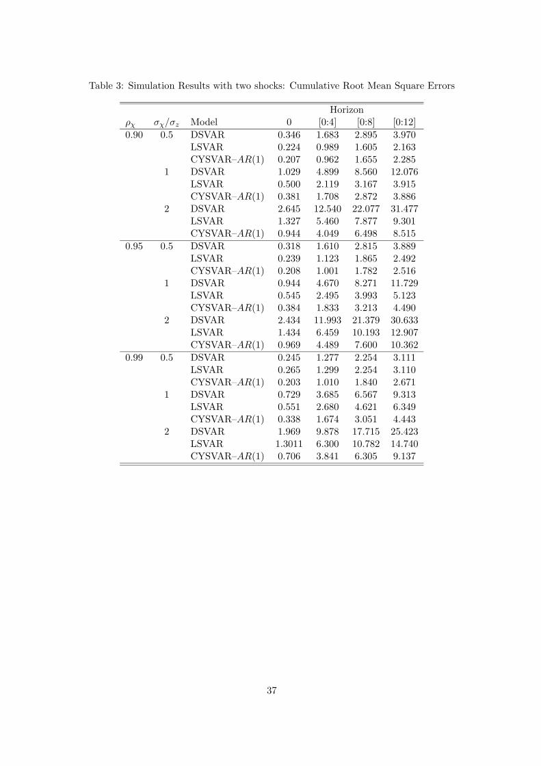
Table 3: Simulation Results with two shocks: Cumulative Root Mean Square Errors

Horizonρχ σχ/σz Model 0 [0:4] [0:8] [0:12]

0.90 0.5 DSVAR 0.346 1.683 2.895 3.970LSVAR 0.224 0.989 1.605 2.163CYSVAR–AR(1) 0.207 0.962 1.655 2.285

1 DSVAR 1.029 4.899 8.560 12.076LSVAR 0.500 2.119 3.167 3.915CYSVAR–AR(1) 0.381 1.708 2.872 3.886

2 DSVAR 2.645 12.540 22.077 31.477LSVAR 1.327 5.460 7.877 9.301CYSVAR–AR(1) 0.944 4.049 6.498 8.515

0.95 0.5 DSVAR 0.318 1.610 2.815 3.889LSVAR 0.239 1.123 1.865 2.492CYSVAR–AR(1) 0.208 1.001 1.782 2.516

1 DSVAR 0.944 4.670 8.271 11.729LSVAR 0.545 2.495 3.993 5.123CYSVAR–AR(1) 0.384 1.833 3.213 4.490

2 DSVAR 2.434 11.993 21.379 30.633LSVAR 1.434 6.459 10.193 12.907CYSVAR–AR(1) 0.969 4.489 7.600 10.362

0.99 0.5 DSVAR 0.245 1.277 2.254 3.111LSVAR 0.265 1.299 2.254 3.110CYSVAR–AR(1) 0.203 1.010 1.840 2.671

1 DSVAR 0.729 3.685 6.567 9.313LSVAR 0.551 2.680 4.621 6.349CYSVAR–AR(1) 0.338 1.674 3.051 4.443

2 DSVAR 1.969 9.878 17.715 25.423LSVAR 1.3011 6.300 10.782 14.740CYSVAR–AR(1) 0.706 3.841 6.305 9.137

37

Table 4: Simulation Results with two shocks: Correlation

ρχ σχ/σz Model Corr(εz, ηT ) Corr(εχ, ηT )

0.90 0.5 DSVAR 0.908 0.325LSVAR 0.937 -0.085CYSVAR 0.943 0.030

1 DSVAR 0.796 0.528LSVAR 0.923 -0.181CYSVAR 0.942 -0.053

2 DSVAR 0.625 0.707LSVAR 0.879 -0.340CYSVAR 0.928 -0.177

0.95 0.5 DSVAR 0.909 0.326LSVAR 0.921 -0.097CYSVAR 0.937 0.044

1 DSVAR 0.799 0.531LSVAR 0.898 -0.215CYSVAR 0.931 -0.047

2 DSVAR 0.626 0.716LSVAR 0.834 -0.404CYSVAR 0.912 -0.189

0.99 0.5 DSVAR 0.921 0.297LSVAR 0.882 -0.068CYSVAR 0.929 0.116

1 DSVAR 0.827 0.498LSVAR 0.853 -0.197CYSVAR 0.917 0.065

2 DSVAR 0.650 0.708LSVAR 0.793 -0.395CYSVAR 0.908 -0.045

38

Table 5: Simulation Results with Three Shocks

Average Cumulative Absolute BiaisHorizon

Variables σg/(σz, σχ) Model 0 0 to 4 0 to 8 0 to 12

(y − h, h) 1 DSVAR 1.037 5.081 8.930 12.568LSVAR 0.286 1.208 1.692 1.832CYSVAR–AR(1) 0.046 0.224 0.413 0.623

2 DSVAR 1.071 5.243 9.216 12.980LSVAR 0.278 1.175 1.652 1.794CYSVAR–AR(1) 0.072 0.343 0.605 0.873

(y − h, h, c − y) 1 DSVAR 0.112 0.555 1.200 2.091LSVAR 0.197 0.805 1.251 1.585CYSVAR–AR(1) 0.046 0.224 0.413 0.623

2 DSVAR 0.151 0.741 1.501 2.468LSVAR 0.198 0.808 1.248 1.560CYSVAR–AR(1) 0.072 0.343 0.605 0.873

Cumulative Root Mean Square ErrorsHorizon

Vairables σg/(σz, σχ) Model 0 0 to 4 0 to 8 0 to 12

(y − h, h) 1 DSVAR 1.064 5.254 9.269 13.084LSVAR 0.531 2.416 3.8547 4.9571CYSVAR–AR(1) 0.392 1.887 3.343 4.688

2 DSVAR 1.097 5.416 9.557 13.499LSVAR 0.544 2.472 3.949 5.083CYSVAR–AR(1) 0.402 1.936 3.436 4.829

(y − h, h, c − y) 1 DSVAR 0.502 2.435 4.261 6.042LSVAR 0.603 2.673 4.190 5.340CYSVAR–AR(1) 0.392 1.887 3.343 4.688

2 DSVAR 0.534 2.575 4.487 6.332LSVAR 0.574 2.570 4.064 5.209CYSVAR–AR(1) 0.402 1.936 3.436 4.829

39

Table 6: Simulation Results with three shocks: Correlation

Variables σg/(σz, σχ) Model Corr(εz, ηT )

(y − h, h) 1 DSVAR 0.774LSVAR 0.904CYSVAR 0.928

2 DSVAR 0.767LSVAR 0.904CYSVAR 0.914

(y − h, h, c − y) 1 DSVAR 0.908LSVAR 0.827CYSVAR 0.928

2 DSVAR 0.898LSVAR 0.817CYSVAR 0.914

40

Figure 1: Data Used in SVARs

1960 1980 2000−0.02

−0.01

0

0.01

0.02

0.03

0.04

Productivity growth

1960 1980 2000

−11.75

−11.7

−11.65

−11.6

−11.55

Hours

1960 1980 2000

−0.56

−0.54

−0.52

−0.5

−0.48

−0.46

Consumption/Output

41

Figure 2: Response of Hours (in logs) to a Positive Technology Shock (two–variables)

(a) Level Specification

0 2 4 6 8 10 12−0.6

−0.4

−0.2

0

0.2

0.4

0.6

0.8

1

1.2

(b) Difference Specification

0 2 4 6 8 10 12−0.8

−0.6

−0.4

−0.2

0

0.2

0.4

0.6

42

Figure 3: Response of Hours (in logs) to a Positive Technology Shock (three–variables)

(a) Level Specification

0 2 4 6 8 10 12−0.6

−0.4

−0.2

0

0.2

0.4

0.6

0.8

1

1.2

(b) Difference Specification

0 2 4 6 8 10 12−0.8

−0.6

−0.4

−0.2

0

0.2

0.4

0.6

43

Figure 4: True and Estimated IRFs of hours with DSVAR and LSVAR (two shocks and bench-mark calibration)

(a) DSVAR

0 2 4 6 8 10 12−1.2

−1

−0.8

−0.6

−0.4

−0.2

0

0.2

0.4IRF of N to a techno shock (Labor in difference)

(b) LSVAR

0 2 4 6 8 10 12−0.6

−0.4

−0.2

0

0.2

0.4

0.6

0.8

1

1.2

1.4IRF of N to a techno shock (Labor in level)

44

Figure 5: True and Estimated IRFs of hours with CYSVARs (two shocks and benchmark cali-bration)

(a) CYSVAR-h

0 2 4 6 8 10 12

−0.4

−0.2

0

0.2

0.4

0.6

0.8

1

1.2

1.4IRF of N to a techno shock (Y/C, N in level)

(b) CYSVAR-∆h

0 2 4 6 8 10 12

−0.4

−0.2

0

0.2

0.4

0.6

0.8

1

1.2

1.4

(c) CYSVAR-AR(1)

0 2 4 6 8 10 12

−0.4

−0.2

0

0.2

0.4

0.6

0.8

1

1.2

1.4

45

Figure 6: Autocorrelation function (preference shock)

0 2 4 6 8 10 120.2

0.3

0.4

0.5

0.6

0.7

0.8

0.9

1HoursC/Y

Figure 7: Autocorrelation function (technology and preference shock)

0 2 4 6 8 10 120.55

0.6

0.65

0.7

0.75

0.8

0.85

0.9

0.95

1

HoursC/YK/Z

46

Figure 8: True and Estimated IRFs of hours with DSVAR, LSVAR and CYSVAR-AR(1) (threeshocks, two variables and benchmark calibration)

(a) DSVAR

0 2 4 6 8 10 12−1.2

−1

−0.8

−0.6

−0.4

−0.2

0

0.2

0.4

0.6IRF of N to a techno shock (Labor in difference)

(b) LSVAR

0 2 4 6 8 10 12−0.4

−0.2

0

0.2

0.4

0.6

0.8

1

1.2

1.4

1.6IRF of N to a techno shock (Labor in level)

(b) CYSVAR-AR(1)

0 2 4 6 8 10 12−0.4

−0.2

0

0.2

0.4

0.6

0.8

1

1.2

1.4

1.6IRF of N to a techno shock (Y/C and a labor lag)

47

Figure 9: True and Estimated IRFs of hours with DSVAR, LSVAR and CYSVAR-AR(1) (threeshocks, three variables and benchmark calibration)

(a) DSVAR

0 2 4 6 8 10 12−0.8

−0.6

−0.4

−0.2

0

0.2

0.4

0.6

0.8

1

1.2IRF of N to a techno shock (Labor in difference)

(b) LSVAR

0 2 4 6 8 10 12

−0.4

−0.2

0

0.2

0.4

0.6

0.8

1

1.2

1.4

1.6IRF of N to a techno shock (Labor in level)

(b) CYSVAR-AR(1)

0 2 4 6 8 10 12

−0.4

−0.2

0

0.2

0.4

0.6

0.8

1

1.2

1.4

1.6IRF of N to a techno shock (Y/C and a labor lag)

48

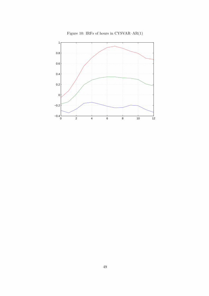
Figure 10: IRFs of hours in CYSVAR–AR(1)

0 2 4 6 8 10 12−0.4

−0.2

0

0.2

0.4

0.6

0.8

1

49

Figure 11: IRFs of hours in LSVAR with breaks in labor productivity

(a) LSVAR

0 2 4 6 8 10 12−1.2

−1

−0.8

−0.6

−0.4

−0.2

0

0.2

0.4

(b) CYSVAR–AR(1)

0 2 4 6 8 10 12−0.8

−0.6

−0.4

−0.2

0

0.2

0.4

0.6

0.8

1

50